Lecture 4: Hypotheses Tests and ConfidenceRegions

Mans Thulin

Department of Mathematics, Uppsala University

thulin@math.uu.se

Multivariate Methods • 6/4 2011

1/24

Outline

I Testing hypotheses in p dimensionsI Hypotheses about µ for the MVN

I Hotelling’s T 2

I Confidence regionsI T 2

I Bonferroni’s inequalities

I Large sample approximations

2/24

Reminder: testing hypotheses

I Hypothesis: null and alternative

I Test statistic

I Quantiles

I Significance level α

I p-value

I Power of test

I t-test, z-test, . . .

3/24

Testing hypotheses in p dimensions

I Several problems occur when we wish to test hypotheses for pdimensional random variables.

I Dependencies between variables makes testing complicatedI Usually we want to test a hypothesis for the p variables’ joint

distribution as well as hypotheses for each of the p marginaldistributions

I The number of parameters in the hypotheses can be largeI A huge number of possible statistics existI Choice between many univariate tests and one multivariate test

I Example: the multivariate normal distribution has 12p(p + 3)

parameters.I For p = 5, the MVN has 20 parametersI For p = 10, the MVN has 65 parametersI For p = 100, the MVN has 5150 parametersI It is difficult to reliably estimate or test hypotheses about all of

these!

4/24

Testing H0 : µ = µ0 – an exampleConsider X = (X1,X2) belonging to a bivariate normal distributionN2(µ,Σ). We wish to test H0 : µ = µ0 = (182, 182).For simplicity, we assume that X1 and X2 are independent and thatboth have a known variance σ2 = 100.

Given 25 observations x1, . . . , x25, with x1 = 185.72 andx2 = 183.84 we could test the hypotheses

H(1)0 : µ1 = 182

H(2)0 : µ2 = 182

with two z-tests with significance level a.The test statistics would be

z1 =X1 − 182

10/√

25∼ N(0, 1) under H0

z2 =X2 − 182

10/√

25∼ N(0, 1) under H0

5/24

Testing H0 : µ = µ0 – an exampleH0 is rejected if either H

(1)0 or H

(2)0 is rejected.

Then, since X1 and X2 are independent,

α(simultaneous) = PH0(H0 is rejected) =

PH0(H(1)0 is rejected) + PH0(H

(2)0 is rejected)−

PH0(H(1)0 is rejected) · PH0(H

(2)0 is rejected) =

P(|z1| > λa/2) + P(|z2| > λa/2)− P(|z1| > λa/2) · P(|z2| > λa/2) =

2a− a2.

Thus a = 1−√

1− α would yield a simultaneous test withsignificance level α.We note that if X1 and X2 were not independent, calculating thesimultaneous significance level could be difficult.

Let α = 0.05. Then a = 1−√

1− α ≈ 0.0253 and λa/2 ≈ 2.24.With x1 = 185.72 and x2 = 183.84 we have that |z1| = 1.86 < 2.24and |z2| = 0.92 < 2.24. Thus the null hypothesis is not rejected.

6/24

Testing H0 : µ = µ0 – an example

On the other hand, if H0 is true, then

z3 =1√2

(z1 + z2) ∼ N(0, 1)

and we could use this to perform a single z-test of the hypothesis.We have that z3 = 1.966. With α = 0.05, we get λα/2 = 1.960, so|z3| > λα/2, which means that we would reject the null hypothesis!

Furthermore, if H0 is true, we also have that

z4 = z21 + z2

2 ∼ χ22.

We could use z4 to test the hypothesis; we get thatz4 = 4.306 < χ2

2(0.05), so the null hypothesis would not berejected.

Which test should we trust? Are there other, better, tests?

7/24

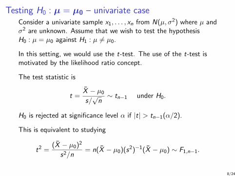
Testing H0 : µ = µ0 – univariate caseConsider a univariate sample x1, . . . , xn from N(µ, σ2) where µ andσ2 are unknown. Assume that we wish to test the hypothesisH0 : µ = µ0 against H1 : µ 6= µ0.

In this setting, we would use the t-test. The use of the t-test ismotivated by the likelihood ratio concept.

The test statistic is

t =X − µ0s/√

n∼ tn−1 under H0.

H0 is rejected at significance level α if |t| > tn−1(α/2).

This is equivalent to studying

t2 =(X − µ0)2

s2/n= n(X − µ0)(s2)−1(X − µ0) ∼ F1,n−1.

8/24

Testing H0 : µ = µ0 – T 2

It would therefore seem natural to study a multivariategeneralization of

t2 =(X − µ0)2

s2/n= n(X − µ0)(s2)−1(X − µ0),

namely,T 2 = n(X− µ0)′S−1(X− µ0).

This statistic is called Hotelling’s T 2 after Harold Hotelling, whoshowed that, under H0,

n − p

(n − 1)p· T 2 ∼ Fp,n−p.

9/24

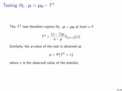
Testing H0 : µ = µ0 – T 2

The T 2 test therefore rejects H0 : µ = µ0 at level α if

T 2 >(n − 1)p

n − pFp,n−p(α).

Similarly, the p-value of the test is obtained as

p = P(T 2 > x)

where x is the observed value of the statistic.

10/24

Testing H0 : µ = µ0 – T 2

Some further remarks regarding Hotelling’s T 2:

I T 2 is invariant under transformations of the kind CX + dwhere X is the data matrix, C is a non-singular matrix and dis a vector.

I Hotelling’s T 2 is the likelihood ratio test (see J&W Sec 5.3)and has some optimality properties.

I Under the alternative H1 : µ = µ1,

n − p

(n − 1)p· T 2 ∼ F

(p, n − p, (µ1 − µ0)′Σ−1(µ1 − µ0)

),

where F (n1, n2,A) is a noncentral F -distribution with degreesof freedom n1 and n2 and noncentrality parameter A. Thepower of the T 2-test against H1 can thus be easily obtained.

11/24

Confidence regions

A (univariate) confidence interval for the parameter θ is an intervalthat covers the true parameter value with probability 1− α (beforesampling).

A confidence region for the p-dimensional parameter θ is a regionin p-dimensional space that covers the true parameter value withprobability 1− α (before sampling).

12/24

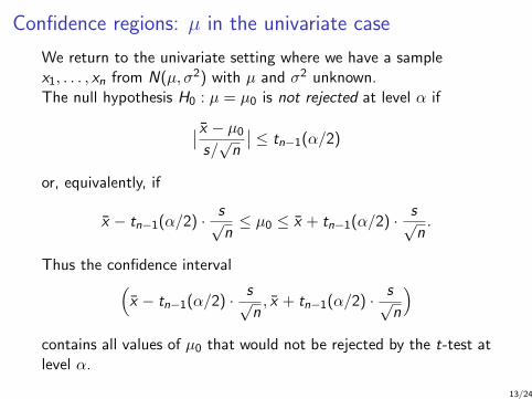
Confidence regions: µ in the univariate case

We return to the univariate setting where we have a samplex1, . . . , xn from N(µ, σ2) with µ and σ2 unknown.The null hypothesis H0 : µ = µ0 is not rejected at level α if∣∣ x − µ0

s/√

n

∣∣ ≤ tn−1(α/2)

or, equivalently, if

x − tn−1(α/2) · s√n≤ µ0 ≤ x + tn−1(α/2) · s√

n.

Thus the confidence interval(x − tn−1(α/2) · s√

n, x + tn−1(α/2) · s√

n

)contains all values of µ0 that would not be rejected by the t-test atlevel α.

13/24

Confidence regions: Confidence ellipses

Analogously, the region

n(X− µ)′S−1(X− µ) ≤ p(n − 1)

n − pFp,n−p(α)

contains the values of µ0 that would not be rejected by Hotelling’sT 2 at level α.

We have that

P(

n(X− µ)′S−1(X− µ) ≤ p(n − 1)

n − pFp,n−p(α)

)= 1− α.

The region above is thus a confidence region for µ. It’s an ellipsoidcentered at x. The axes of the ellipsoid are given by theeigenvectors of S.

See figure on blackboard!

14/24

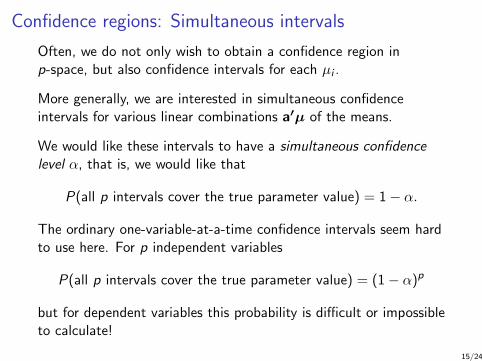
Confidence regions: Simultaneous intervals

Often, we do not only wish to obtain a confidence region inp-space, but also confidence intervals for each µi .

More generally, we are interested in simultaneous confidenceintervals for various linear combinations a′µ of the means.

We would like these intervals to have a simultaneous confidencelevel α, that is, we would like that

P(all p intervals cover the true parameter value) = 1− α.

The ordinary one-variable-at-a-time confidence intervals seem hardto use here. For p independent variables

P(all p intervals cover the true parameter value) = (1− α)p

but for dependent variables this probability is difficult or impossibleto calculate!

15/24

Confidence regions: Simultaneous intervals

Result 5.3. Let X1, . . . ,Xn be a random sample from N(µ,Σ),where Σ is positive definite. Then

(a′X−

√p(n − 1)

(n − p)Fp,n−p(α)

a′Sa

n, a′X+

√p(n − 1)

(n − p)Fp,n−p(α)

a′Sa

n

)contains a′µ with probability 1− α simultaneously for all a.

The part under the square root comes from the distribution of theT 2 statistic.

Taking a′ = (1, 0, . . . , 0), a′ = (0, 1, 0, . . . , 0), . . .,a′ = (0, 0, . . . , 0, 1) gives us simultaneous intervals for µ1, . . . , µn.Taking a′ = (1,−1, 0 . . . , 0) gives us an interval for µ1 − µ2, andso on.

Proof of Res 5.3: see blackboard!

16/24

Confidence regions: One-at-a-time intervals

From the previous slide, the simultaneous confidence interval for µiis (

xi ±

√p(n − 1)

(n − p)Fp,n−p(α)

√siin

)How does this compare to the ordinary one-at-a-time confidenceinterval (

xi ± tn−1(α/2)

√siin

)?

To compare the intervals, we need only to compare√p(n−1)(n−p) Fp,n−p(α) and tn−1(α/2).

17/24

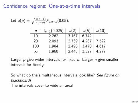
Confidence regions: One-at-a-time intervals

Let a(p) =√

p(n−1)(n−p) Fp,n−p(0.05).

n tn−1(0.025) a(2) a(5) a(10)

10 2.262 3.167 6.742 –20 2.093 2.739 4.287 7.522

100 1.984 2.498 3.470 4.617∞ 1.960 2.448 3.327 4.277

Larger p give wider intervals for fixed n. Larger n give smallerintervals for fixed p.

So what do the simultaneous intervals look like? See figure onblackboard!The intervals cover to wide an area!

18/24

Confidence regions: Bonferroni intervals

Bonferroni’s inequalities is a set of inequalities for probabilities ofunions of events.Let C1, . . . ,Cp be confidence intervals, with P(Ci covers the trueparameter value) = 1− αi .The Bonferroni inequality for confidence intervals is:

P(all Ci cover the true parameter values) ≥ 1− (α1 + . . .+ αp)

Proof: see blackboard.

Typically, αi = α/p is choosen. Then P(all Ci cover the trueparameter value) ≥ 1− α and the Bonferroni simultaneousconfidence interval for µi is(

xi ± tn−1( α

2p

)√siin

).

19/24

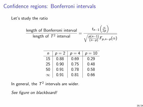
Confidence regions: Bonferroni intervals

Let’s study the ratio

length of Bonferroni interval

length of T 2 interval=

tn−1(α2p

)√

p(n−1)(n−p) Fp,n−p(α)

n p = 2 p = 4 p = 10

15 0.88 0.69 0.2925 0.90 0.75 0.4850 0.91 0.78 0.58∞ 0.91 0.81 0.66

In general, the T 2 intervals are wider.

See figure on blackboard!

20/24

Bonferroni inequality for tests

Similarly, a Bonferroni inequality can be stated for tests.We wish to perform m test with a simultaneous significance levelα. Let P1, . . . ,Pm be the p-values for the m tests.Then

P( m⋃

i=1

(Pi ≤ α/m))≤ α.

That is, the probability of rejecting at least one hypothesis whenall hypotheses are true is no greater than α. Thus thesimultaneous significance level is at most α.

The Bonferroni inequlity for tests is useful when we wish to testhypotheses about different variables simultaneously (for instancewhen testing for marginal normality).

(An extension of this idea is studied in homework 2.)

21/24

Large sample approximations

For large n, the methods we’ve discussed for normal data can oftenbe used even if the data is non-normal.

For multivariate distributions with finite Σ, the multivariate centrallimit theorem can be used together with Cramers lemma (alsoknown as Slutsky’s lemma) to show that

T 2 d−→ χ2p

so that

P(

T 2 ≤ χ2p(α)

)= P

(n(X− µ)′S−1(X− µ) ≤ χ2

p(α))≈ 1− α

when n is sufficiently large.

22/24

Large sample approximations

Thus, the large sample T 2 test rejects H0 : µ = µ0 if

T 2 = n(X− µ0)′S−1(X− µ0) > χ2p(α).

It also follows that, simultaneously for all a,

(a′X±

√χ2p(α)

√a′Sa

n

)contains a′µ with probability approximately 1− α.Finally, the Bonferroni simultaneous confidence intervals for the µiare obtained using the univariate central limit theorem:(

xi ± λ( α

2p

)√siin

).

where λ( α2p

)are the quantiles from the standard normal

distribution.23/24

Summary

I Testing hypotheses in p dimensionsI Hypotheses about µ for the MVN

I Hotelling’s T 2

I Analogue to t-test

I Confidence regionsI T 2

I Bonferroni’s inequalities

I Large sample approximations

24/24