Statistics for Business and Economics

Chapter 7 Inferences Based on Two Samples:

Confidence Intervals & Tests of Hypotheses

Learning Objectives

1. Distinguish Independent and Related Populations

2. Solve Inference Problems for Two Populations

• Mean • Proportion• Variance

3. Determine Sample Size

Thinking Challenge

• Who gets higher grades: males or females?

• Which program is faster to learn: Word or Excel?

How would you try to answer these questions?

Target Parameters

Difference between Means –

Difference between Proportions

p– p

Ratio of Variances2

12

2

( )

( )

Independent & Related Populations

1. Different data sources• Unrelated

• Independent

Independent Related1. Same data source

• Paired or matched

• Repeated measures (before/after)

2. Use difference between each pair of observations

• di = x1i – x2i

2. Use difference between the two sample means

• X1 – X2

Two Independent Populations Examples

1. An economist wishes to determine whether there is a difference in mean family income for households in two socioeconomic groups.

2. An admissions officer of a small liberal arts college wants to compare the mean SAT scores of applicants educated in rural high schools and in urban high schools.

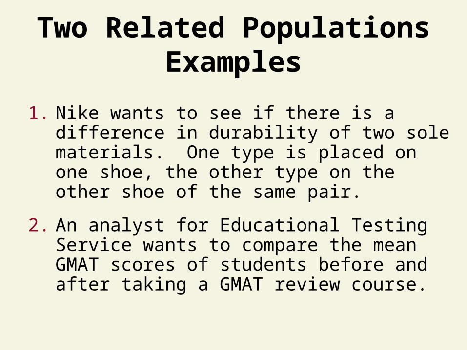
Two Related Populations Examples

1. Nike wants to see if there is a difference in durability of two sole materials. One type is placed on one shoe, the other type on the other shoe of the same pair.

2. An analyst for Educational Testing Service wants to compare the mean GMAT scores of students before and after taking a GMAT review course.

Thinking Challenge

1. Miles per gallon ratings of cars before and after mounting radial tires

2. The life expectancy of light bulbs made in two different factories

3. Difference in hardness between two metals: one contains an alloy, one doesn’t

4. Tread life of two different motorcycle tires: one on the front, the other on the back

Are they independent or related?

Two Population Inference

TwoPopulations

Z (Large

sample)

t(Pairedsample)

Z

Proportion Variance

F t

(Smallsample)

Paired

Indep.

Mean

Comparing Two Means

Two Population Inference

TwoPopulations

Z (Large

sample)

t(Pairedsample)

Z

Proportion Variance

F t

(Smallsample)

Paired

Indep.

Mean

Comparing Two Independent Means

Two Population Inference

TwoPopulations

Z (Large

sample)

t(Pairedsample)

Z

Proportion Variance

F t

(Smallsample)

Paired

Indep.

Mean

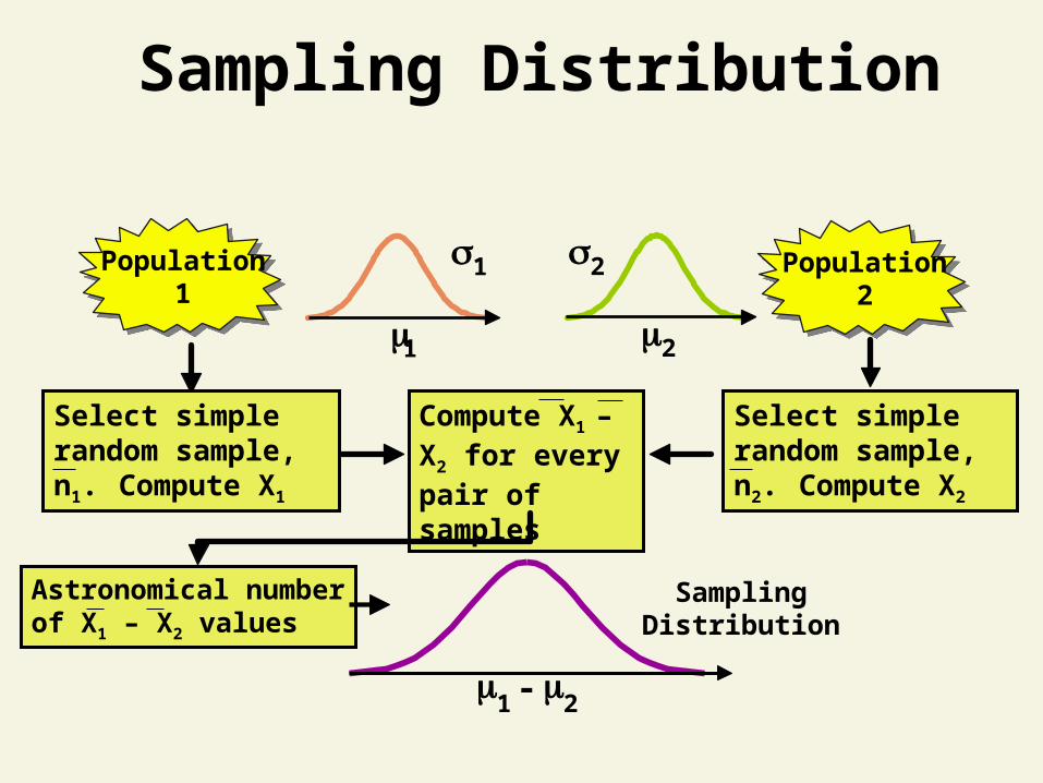
Sampling Distribution

Population1

1

1

Select simple random sample, n1. Compute X1

Compute X1 – X2 for every pair of samples

Population2

2

2

Select simple random sample, n2. Compute X2

Astronomical numberof X1 – X2 values

1 - 2

SamplingDistribution

Large-Sample Inference for Two Independent Means

Two Population Inference

TwoPopulations

Z (Large

sample)

t(Pairedsample)

Z

Proportion Variance

F t

(Smallsample)

Paired

Indep.

Mean

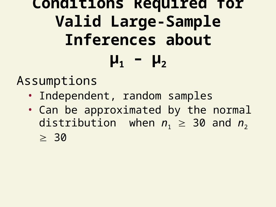
Conditions Required for Valid Large-Sample Inferences about

μ1 – μ2

Assumptions• Independent, random samples• Can be approximated by the normal distribution

when n1 30 and n2 30

Large-Sample Confidence Interval for μ1 – μ2

(Independent Samples)

Confidence Interval

2 21 2

1 2 21 2

X X Zn n

Large-Sample Confidence Interval Example

You’re a financial analyst for Charles Schwab. You want to estimate the difference in dividend yield between stocks listed on NYSE and NASDAQ. You collect the following data: NYSE NASDAQNumber 121 125Mean 3.27 2.53Std Dev 1.30 1.16What is the 95% confidence intervalfor the difference between the mean dividend yields?

© 1984-1994 T/Maker Co.

Large-Sample Confidence Interval Solution

2 21 2

1 2 21 2

2 2

1 2

(1.3) (1.16)(3.27 2.53) 1.96

121 125

.43 1.05

X X Zn n

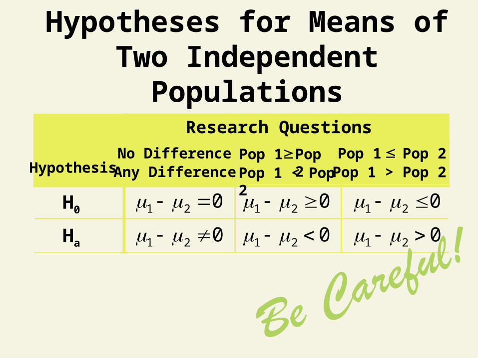
Hypotheses for Means of Two Independent Populations

Ha

Hypothesis

Research Questions

No DifferenceAny Difference

Pop 1

Pop 2Pop 1 < Pop 2

Pop 1 Pop 2Pop 1 > Pop 2

H0 1 2 0

1 2 0 1 2 0

1 2 0 1 2 0

1 2 0

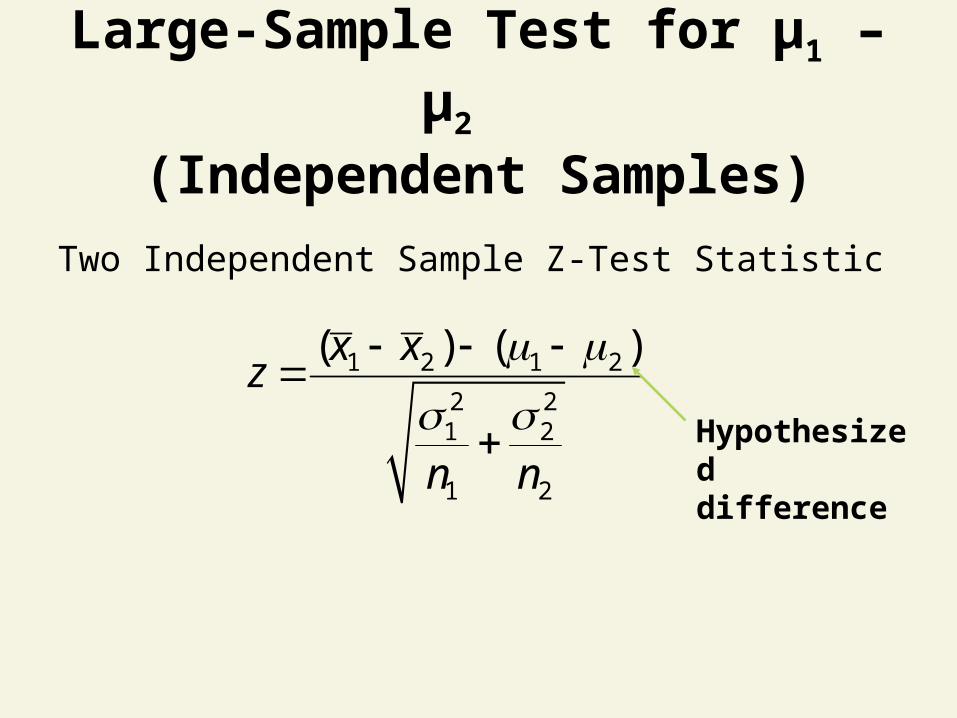
Large-Sample Test for μ1 – μ2 (Independent Samples)

Two Independent Sample Z-Test Statistic

1 2 1 2

2 21 2

1 2

( ) ( )x xz

n n

Hypothesized difference

Large-Sample Test Example

You’re a financial analyst for Charles Schwab. You want to find out if there is a difference in dividend yield between stocks listed on NYSE and NASDAQ. You collect the following data: NYSE NASDAQNumber 121 125Mean 3.27 2.53Std Dev 1.30 1.16Is there a difference in average yield ( = .05)?

© 1984-1994 T/Maker Co.

Large-Sample Test Solution

• H0:• Ha:• • n1= , n2 =• Critical Value(s):

Test Statistic:

Decision:

Conclusion:

.05

121 125

(3.27 2.53) 04.69

1.698 1.353121 125

z

Reject at = .05

There is evidence of a difference in meansz0 1.96-1.96

Reject H0 Reject H0

.025 .025

1 - 2 = 0 (1 = 2)

1 - 2 0 (1 2)

You’re an economist for the Department of Education. You want to find out if there is a difference in spending per pupil between urban and rural high schools. You collect the following: Urban Rural Number 35 35Mean $ 6,012 $ 5,832Std Dev $ 602 $ 497Is there any difference in population means ( = .10)?

Large-Sample Test Thinking Challenge

Large-Sample Test Solution*

• H0:• Ha:• • n1 = , n2 =• Critical Value(s):

Test Statistic:

Decision:

Conclusion:

Do not reject at = .10

There is no evidence of a difference in meansz0 1.645-1.645

.05

Reject H0 Reject H0

.05

2 2

(6012 5832) 01.36

602 49735 35

z

1 - 2 = 0 (1 = 2)

1 - 2 0 (1 2).10

35 35

Small-Sample Inference for Two Independent Means

Two Population Inference

TwoPopulations

Z (Large

sample)

t(Pairedsample)

Z

Proportion Variance

F t

(Smallsample)

Paired

Indep.

Mean

Conditions Required for Valid Small-Sample Inferences about

μ1 – μ2

Assumptions• Independent, random samples• Populations are approximately normally distributed• Population variances are equal

Small-Sample Confidence Interval for μ1 – μ2

(Independent Samples)

Confidence Interval

21 2 2

1 2

2 22 1 1 2 2

1 2

1 2

1 1

1 1

2

2

P

P

X X t Sn n

n S n SS

n n

df n n

Small-Sample Confidence Interval Example

You’re a financial analyst for Charles Schwab. You want to estimate the difference in dividend yield between stocks listed on the NYSE and NASDAQ? You collect the following data: NYSE NASDAQNumber 11 15Mean 3.27 2.53Std Dev 1.30 1.16Assuming normal populations, what is the 95% confidence intervalfor the difference between the mean dividend yields?

© 1984-1994 T/Maker Co.

Small-Sample Confidence Interval Solution

2 22 1 1 2 2

1 2

2 2

1 1

2

11 1 1.30 15 1 1.161.489

11 15 2

P

n S n SS

n n

1 2

1 13.27 2.53 2.064 1.489

11 15

.26 1.74

df = n1 + n2 – 2 = 11 + 15 – 2 = 24 t.025 = 2.064

Two Independent Sample t–Test Statistic

2

2

11

11

21

21

222

2112

21

2

2121

nndf

nn

SnSnS

nnS

XXt

P

P

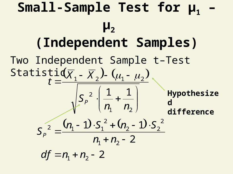
Small-Sample Test for μ1 – μ2 (Independent Samples)

Hypothesized difference

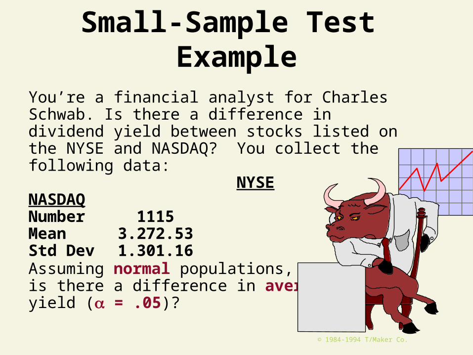
Small-Sample Test Example

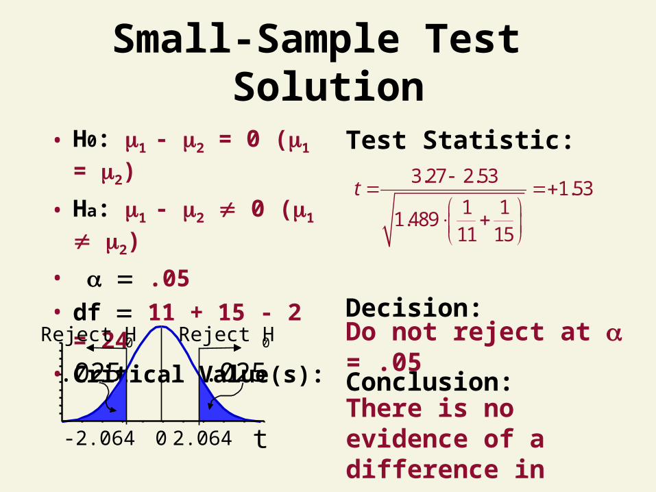
You’re a financial analyst for Charles Schwab. Is there a difference in dividend yield between stocks listed on the NYSE and NASDAQ? You collect the following data: NYSE NASDAQNumber 11 15Mean 3.27 2.53Std Dev 1.30 1.16Assuming normal populations, is there a difference in average yield ( = .05)?

© 1984-1994 T/Maker Co.

• H0:• Ha:• • df • Critical Value(s):

Test Statistic:

Decision:

Conclusion:

1 - 2 = 0 (1 = 2)

1 - 2 0 (1 2)

.05

11 + 15 - 2 = 24

t0 2.064-2.064

.025

Reject H 0 Reject H0

.025

Small-Sample Test Solution

Small-Sample Test Solution

2 22 1 1 2 2

1 2

2 2

1 1

2

11 1 1.30 15 1 1.161.489

11 15 2

P

n S n SS

n n

1 2 1 2

2

1 2

3.27 2.53 01.53

1 11 1 1.48911 15P

X Xt

Sn n

• H0: 1 - 2 = 0 (1 = 2)

• Ha: 1 - 2 0 (1 2)

• .05• df 11 + 15 - 2 = 24• Critical Value(s):

Test Statistic:

Decision:

Conclusion:

3.27 2.531.53

1 11.489

11 15

t

Do not reject at = .05

There is no evidence of a difference in meanst0 2.064-2.064

.025

Reject H 0 Reject H0

.025

Small-Sample Test Solution

You’re a research analyst for General Motors. Assuming equal variances, is there a difference in the average miles per gallon (mpg) of two car models ( = .05)?

You collect the following:

Sedan Van

Number 15 11Mean 22.00 20.27Std Dev 4.77 3.64

Small-Sample Test Thinking Challenge

• H0: • Ha:• • df • Critical Value(s):

Test Statistic:

Decision:

Conclusion:

t0 2.064-2.064

.025

Reject H 0 Reject H0

.025

1 - 2 = 0 (1 = 2)

1 - 2 0 (1 2)

.05

15 + 11 - 2 = 24

Small-Sample Test Solution*

2 22 1 1 2 2

1 2

2 2

1 1

2

15 1 4.77 11 1 3.6418.793

15 11 2

P

n S n SS

n n

1 2 1 2

2

1 2

22.00 20.27 01.00

1 11 1 18.79315 11P

X Xt

Sn n

Small-Sample Test Solution*

Test Statistic:

Decision:

Conclusion:

22.00 20.271.00

1 118.793

15 11

t

Do not reject at = .05

There is no evidence of a difference in means

Small-Sample Test Solution*

• H0: • Ha:• • df • Critical Value(s):

t0 2.064-2.064

.025

Reject H 0 Reject H0

.025

1 - 2 = 0 (1 = 2)

1 - 2 0 (1 2)

.05

15 + 11 - 2 = 24

Paired Difference Experiments

Small-Sample

Two Population Inference

TwoPopulations

Z (Large

sample)

t(Pairedsample)

Z

Proportion Variance

F t

(Smallsample)

Paired

Indep.

Mean

Paired-Difference Experiments

1. Compares means of two related populations• Paired or matched• Repeated measures (before/after)

2. Eliminates variation among subjects

Conditions Required for Valid Small-Sample Paired-Difference

Inferences

Assumptions• Random sample of differences• Both population are approximately normally

distributed

Paired-Difference Experiment Data Collection Table

Observation Group 1 Group 2 Difference

1 x11 x21 d1 = x11 – x21

2 x12 x22 d2 = x12 – x22

i x1i x2i di = x1i – x2i

n x1n x2n dn = x1n – x2n

Paired-Difference Experiment Small-Sample Confidence

Interval

Sample Mean Sample Standard Deviation

d

d

nS

(di - d)2

n

ii

n

di

n

1 1

1d d

df = nd – 12d

d

sd t

n

Paired-Difference Experiment Confidence Interval Example

You work in Human Resources. You want to see if there is a difference in test scores after a training program. You collect the following test score data:

Name Before (1) After (2)

Sam 85 94Tamika 94 87Brian 78 79Mike 87 88

Find a 90% confidence interval for themean difference in test scores.

Computation Table

Observation Before After Difference

Sam 85 94 -9

Tamika 94 87 7

Brian 78 79 -1

Mike 87 88 -1

Total - 4

d = –1 Sd = 6.53

Paired-Difference Experiment Confidence Interval Solution

2

6.531 2.353

48.68 6.68

d

d

d

Sd t

n

df = nd – 1 = 4 – 1 = 3 t.05 = 2.353

Hypotheses for Paired-Difference Experiment

Ha

Hypothesis

Research Questions

No DifferenceAny Difference

Pop 1

Pop 2Pop 1 < Pop 2

Pop 1 Pop 2Pop 1 > Pop 2

H00d

0d

0d 0d

0d

Note: di = x1i – x2i for ith observation

0d

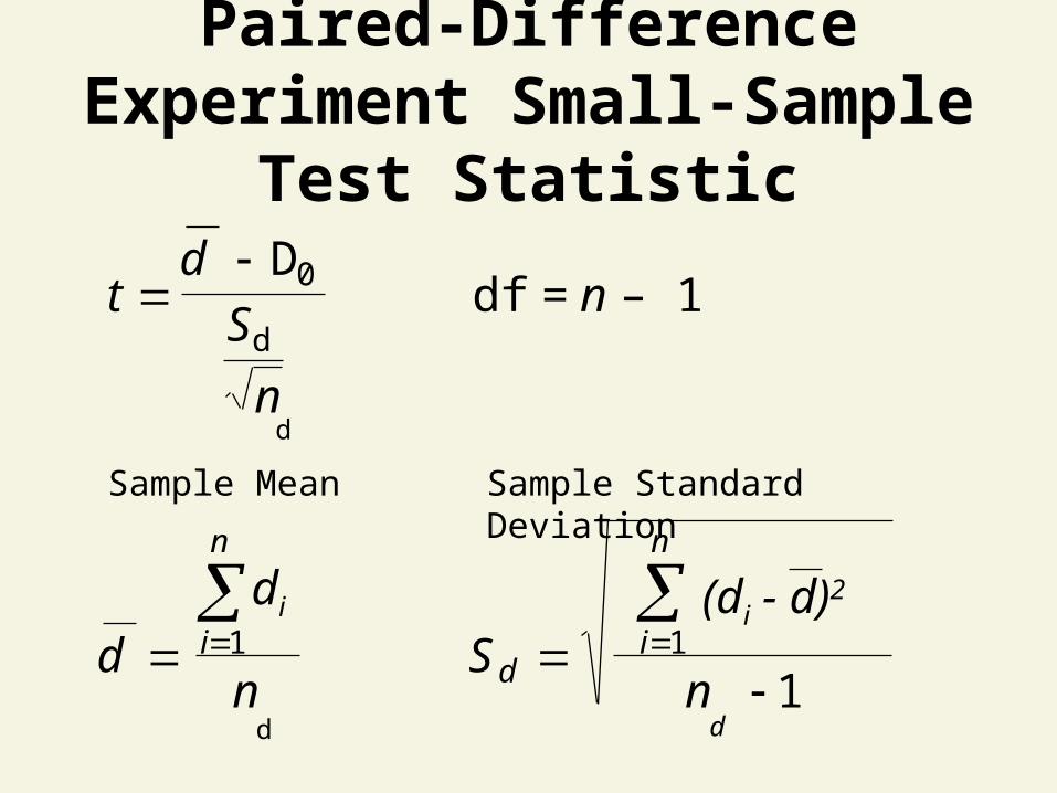
Paired-Difference Experiment Small-Sample Test Statistic

td

S

n

df = n – 10

d

D

d

Sample Mean Sample Standard Deviation

d

di

nS

(di - d)2

ni

n

di

n

1 1

1d d

Paired-Difference Experiment Small-Sample Test Example

You work in Human Resources. You want to see if a training program is effective. You collect the following test score data:

Name Before After

Sam 85 94Tamika 94 87Brian 78 79Mike 87 88

At the .10 level of significance, was the training effective?

Null HypothesisSolution

1. Was the training effective?

2. Effective means ‘Before’ < ‘After’.

3. Statistically, this means B < A.

4. Rearranging terms gives B – A < 0.

5. Defining d = B – A and substituting into (4) gives d .

6. The alternative hypothesis is Ha: d 0.

Paired-Difference Experiment Small-Sample Test Solution

• H0:• Ha:

• = • df =• Critical Value(s):

Test Statistic:

Decision:

Conclusion:

d = 0 (d = B - A)

d < 0

.10

4 - 1 = 3

t0-1.638

.10

Reject H0

Computation Table

Observation Before After Difference

Sam 85 94 -9

Tamika 94 87 7

Brian 78 79 -1

Mike 87 88 -1

Total - 4

d = –1 Sd = 6.53

Paired-Difference Experiment Small-Sample Test Solution

• H0:• Ha:

• = • df =• Critical Value(s):

Test Statistic:

Decision:

Conclusion:

d = 0 (d = B - A)

d < 0

.10

4 - 1 = 3

t0-1.638

.10

Reject H0 Do not reject at = .10

There is no evidence training was effective

0 1 0.306

6.53

4d

d

d Dt

S

n

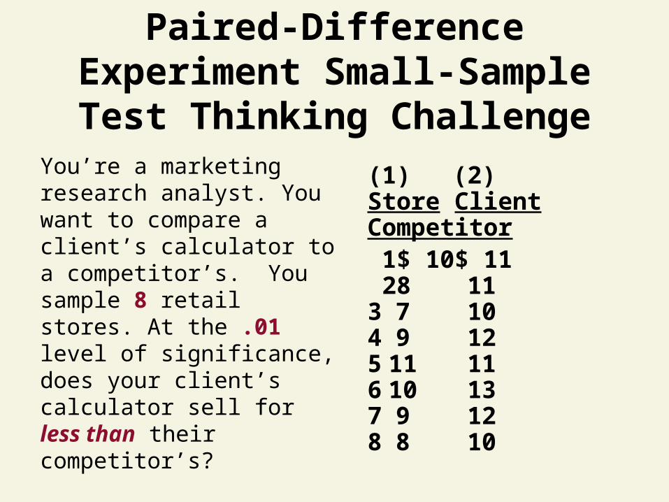
Paired-Difference Experiment Small-Sample Test Thinking

ChallengeYou’re a marketing research analyst. You want to compare a client’s calculator to a competitor’s. You sample 8 retail stores. At the .01 level of significance, does your client’s calculator sell for less than their competitor’s?

(1) (2)Store Client Competitor

1$ 10 $ 11 2 8 11

3 7 104 9 125 11 116 10 137 9 128 8 10

Paired-Difference Experiment Small-Sample Test Solution*

• H0:• Ha:• =• df =• Critical Value(s):

Test Statistic:

Decision:

Conclusion:

Reject at = .01

There is evidence client’s brand (1) sells for lesst0-2.998

.01

Reject H0

0 2.25 05.486

1.16

8d

d

d Dt

S

n

d = 0 (d = 1 - 2)

d < 0

.01

8 - 1 = 7

Comparing Two Population Proportions

Two Population Inference

TwoPopulations

Z (Large

sample)

t(Pairedsample)

Z

Proportion Variance

F t

(Smallsample)

Paired

Indep.

Mean

Conditions Required for Valid Large-Sample Inference about

p1 – p2

Assumptions• Independent, random samples• Normal approximation can be used if

1 1 1 1 2 2 2 2ˆ ˆ ˆ ˆ15, 15, 15, and 15n p n q n p n q

Large-Sample Confidence Interval for p1 – p2

Confidence Interval

1 1 2 21 2 2

1 2

ˆ ˆ ˆ ˆˆ ˆ

p q p qp p Z

n n

Confidence Interval for p1 – p2 Example

As personnel director, you want to test the perception of fairness of two methods of performance evaluation. 63 of 78 employees rated Method 1 as fair. 49 of 82 rated Method 2 as fair. Find a 99% confidence interval for the difference in perceptions.

Confidence Interval for p1 – p2 Solution

1 1

2 2

63ˆ ˆ.808 1 .808 .192

7849

ˆ ˆ.598 1 .598 .40282

p q

p q

1 2

.808 .192 .598 .402.808 .598 2.58

78 82.029 .391p p

Hypotheses for Two Proportions

Ha

Hypothesis

Research Questions

No DifferenceAny Difference

Pop 1

Pop 2Pop 1 < Pop 2

Pop 1 Pop 2Pop 1 > Pop 2

H0 1 2 0p p

1 2 0p p 1 2 0p p

1 2 0p p 1 2 0p p

1 2 0p p

Large-Sample Test for p1 – p2

Z-Test Statistic for Two Proportions

1 2 1 2 1 2

1 2

1 2

ˆ ˆˆwhere

1 1ˆ ˆ

p p p p X XZ p

n npq

n n

Test for Two Proportions Example

As personnel director, you want to test the perception of fairness of two methods of performance evaluation. 63 of 78 employees rated Method 1 as fair. 49 of 82 rated Method 2 as fair. At the .01 level of significance, is there a difference in perceptions?

• H0: • Ha: • =

• n1 = n2 =

• Critical Value(s):

Test Statistic:

Decision:

Conclusion:

p1 - p2 = 0

p1 - p2 0

.0178 82

z0 2.58-2.58

Reject H0 Reject H0

.005 .005

Test for Two Proportions Solution

1 21 2

1 2

1 2

1 2

63 49ˆ ˆ.808 .598

78 82

63 49ˆ .70

78 82

X Xp p

n n

X Xp

n n

Test for Two Proportions Solution

1 2 1 2

1 2

ˆ ˆ .808 .598 0

1 11 1 .70 1 .70ˆ ˆ178 82

2.90

p p p pZ

p pn n

Test Statistic:

Decision:

Conclusion:

Reject at = .01

There is evidence of a difference in proportions

Test for Two Proportions Solution

• H0: • Ha: • =

• n1 = n2 =

• Critical Value(s):

p1 - p2 = 0

p1 - p2 0

.0178 82

z0 2.58-2.58

Reject H0 Reject H0

.005 .005

Z = +2.90

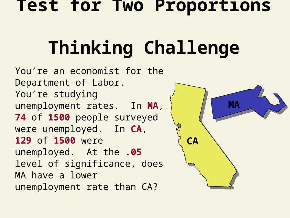
Test for Two Proportions Thinking Challenge

You’re an economist for the Department of Labor. You’re studying unemployment rates. In MA, 74 of 1500 people surveyed were unemployed. In CA, 129 of 1500 were unemployed. At the .05 level of significance, does MA have a lower unemployment rate than CA?

MA

CA

Test Statistic:

Decision:

Conclusion:

• H0:• Ha:• =

• nMA = nCA =

• Critical Value(s):

pMA – pCA = 0

pMA – pCA < 0

.05

1500 1500

Z0-1.645

.05

Reject H0

Test for Two Proportions Solution*

Test for Two Proportions Solution*

74 129ˆ ˆ.0493 .0860

1500 1500

74 129ˆ .0677

1500 1500

CAMAMA CA

MA CA

MA CA

MA CA

XXp p

n n

X Xp

n n

.0493 .0860 0

1 1.0677 1 .0677

1500 1500

4.00

Z

Test Statistic:

Decision:

Conclusion:

Z = –4.00

Reject at = .05

There is evidence MA is less than CA

Test for Two Proportions Solution*

• H0:• Ha:• =

• nMA = nCA =

• Critical Value(s):

pMA – pCA = 0

pMA – pCA < 0

.05

1500 1500

Z0-1.645

.05

Reject H0

Determining Sample Size

Determining Sample Size

• Sample size for estimating μ1 – μ2

• Sample size for estimating p1 – p2

2 2 22 1 2

1 2 2( )

Zn n

ME

2

2 1 1 2 2

1 2 2( )

Z p q p qn n

ME

ME = Margin of Error

Sample Size Example

What sample size is needed to estimate μ1 – μ2 with 95% confidence and a margin of error of 5.8? Assume prior experience tells us σ1 =12 and σ2 =18.

2 2 2

1 2 2

1.96 12 1853.44 54

(5.8)n n

Sample Size Example

What sample size is needed to estimate p1 – p2 with 90% confidence and a width of .05?

2

1 2 2

1.645 .5 .5 .5 .52164.82 2165

(.025)n n

.05.025

2 2

widthME

Comparing Two Population Variances

Two Population Inference

TwoPopulations

Z (Large

sample)

t(Pairedsample)

Z

Proportion Variance

F t

(Smallsample)

Paired

Indep.

Mean

Sampling Distribution

Population1

1

1

Select simple random sample, size n1.

Compute S12

Population2

2

2

Select simple random sample, size n2.

Compute S22

SamplingDistributions forDifferent Sample

Sizes

Astronomical number

of S12/S2

2 values

Compute F = S12/S2

2 for every pair of n1 & n2 size samples

Conditions Required for a Valid F-Test for Equal Variances

Assumptions• Both populations are normally distributed

— Test is not robust to violations

• Independent, random samples

F-Test for Equal Variances Hypotheses

• HypothesesH0: 1

2 = 22 OR H0: 1

2 22 (or )

Ha: 12 2

2 Ha: 12 2

2 (or >)

• Test Statistic• F = s1

2 /s22

• Two sets of degrees of freedom—1 = n1 – 1; 2 = n2 – 1

• Follows F distribution

F-Test for Equal Variances Critical Values

0

Reject H0

Do NotReject H0

F

Reject H0

FFL

U( / ; , )

( / ; , )

2

21 2

2 1

1

Note!

FU ( / ; , ) 2 1 2

/2/2/2/2

F-Test for Equal Variances Example

You’re a financial analyst for Charles Schwab. You want to compare dividend yields between stocks listed on the NYSE & NASDAQ. You collect the following data: NYSE NASDAQNumber 21 25Mean 3.27 2.53Std Dev 1.30 1.16Is there a difference in variances between the NYSE & NASDAQ at the .05 level of significance?

© 1984-1994 T/Maker Co.

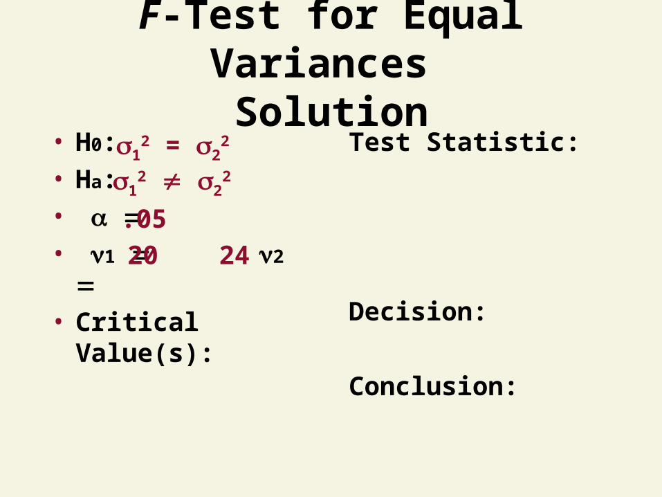
F-Test for Equal Variances Solution

• H0: • Ha:• • 1 2 • Critical Value(s):

Test Statistic:

Decision:

Conclusion:

12 = 2

2

12 2

2

.05

20 24

F-Test for Equal Variances Solution

0

Reject H0

Do NotReject H0

F

Reject H0

415.41.2

11

)20,24;025(.)24,20;025(.

UL F

F

33.2)24,20;025(. UF

/2 = .025/2 = .025

F-Test for Equal Variances Solution

• H0: 12 = 2

2

• Ha: 12 2

2

• .05• 1 20 2 24 • Critical Value(s):

Test Statistic:

Decision:

Conclusion:

2 21

2 22

1.301.25

1.16

SF

S

0 F2.33.415

.025

Reject H0 Reject H0

.025

Do not reject at = .05

There is no evidence of a difference in variances

F-Test for Equal Variances Thinking Challenge

You’re an analyst for the Light & Power Company. You want to compare the electricity consumption of single-family homes in two towns. You compute the following from a sample of homes:

Town 1 Town 2Number 25 21Mean $ 85 $ 68Std Dev $ 30 $ 18At the .05 level of significance, is there evidenceof a difference in variances between the two towns?

F-Test for Equal Variances Solution*

• H0:• Ha:• • 1 2 • Critical Value(s):

Test Statistic:

Decision:

Conclusion:

12 = 2

2

12 2

2

.05

24 20

Critical ValuesSolution*

0

Reject H0

Do NotReject H0

F

Reject H0

429.33.2

11

)24,20;025(.)20,24;025(.

UL F

F

41.2)20,24;025(. UF

/2 = .025/2 = .025

F-Test for Equal Variances Solution*

• H0: 12 = 2

2

• Ha: 12 2

2

• .05• 1 24 2 20 • Critical Value(s):

Test Statistic:

Decision:

Conclusion:

2 21

2 22

302.778

18

SF

S

Reject at = .05

There is evidence of a difference in variances0 F2.41.429

.025

Reject H0 Reject H0

.025

Conclusion

1. Distinguished Independent and Related Populations

2. Solved Inference Problems for Two Populations

• Mean • Proportion• Variance

3. Determined Sample Size