lecture 3: supply and demand - agsm slightly differentiated goods or services. ... ice-cream price...
TRANSCRIPT

Lecture 3 A G S M © 2004 Page 1
LECTURE 3: SUPPLY AND DEMANDToday’s Topics1. Markets and competition.2. Demand: determinants, ceteris paribus,
individual choice , schedule and curve ,individual and market, shifts in demandcur ve.
3. Supply: determinants, schedule and curve ,individual and market, shifts in supply cur ve.
4. Supply and Demand: equilibrium price &quantity, analysing chang es in equilibrium.
>

Lecture 3 A G S M © 2004 Page 2
MARKETS & COMPETITION
A market: a group of buyers and sellers of a goodor service .
Can be more or less organised.
A competitive market: many buyers and sellers sonone has a significant impact on the price.
How do buyers and sellers interact in a competitivemarket? The forces of supply and demanddetermine the quantity sold and its price.
< >
Lecture 3 A G S M © 2004 Page 3
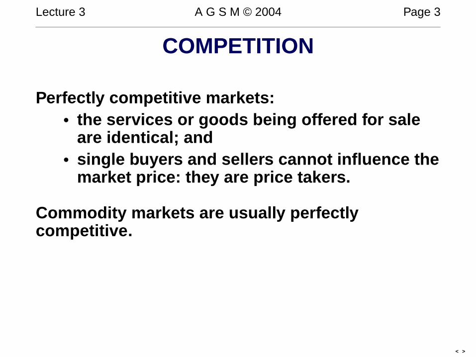
COMPETITION
Perfectly competitive markets:• the services or goods being offered for sale
are identical; and• single buyers and sellers cannot influence the
market price: they are price takers.
Commodity markets are usually perfectlycompetitive .
< >
Lecture 3 A G S M © 2004 Page 4
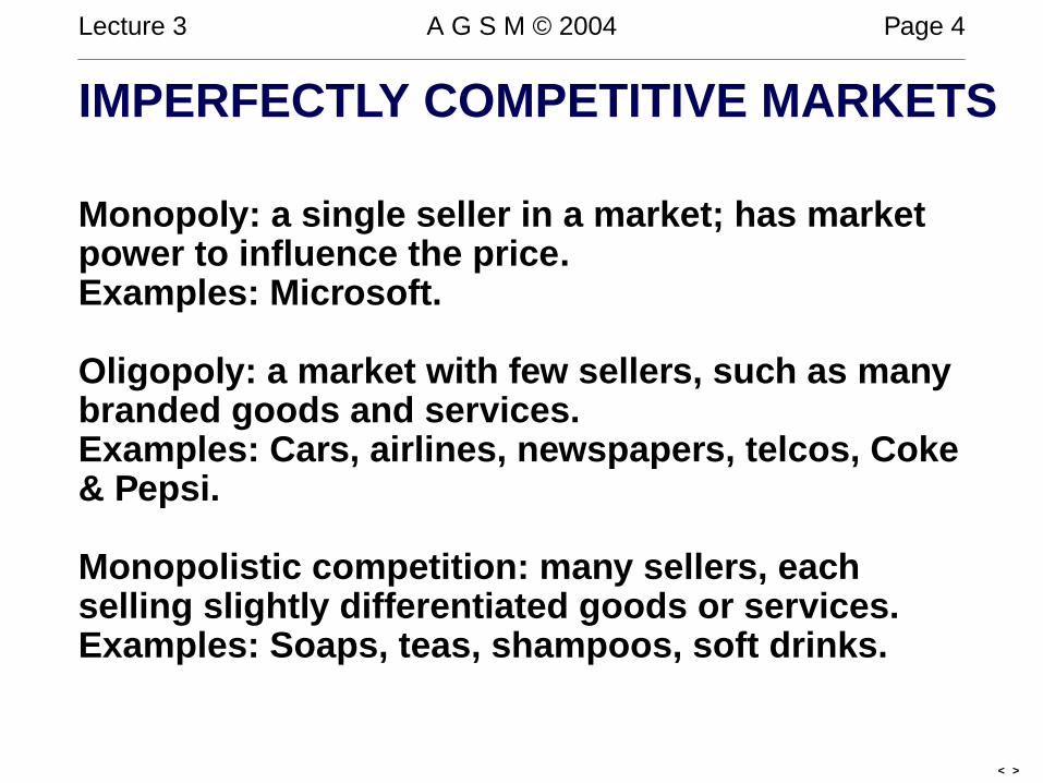
IMPERFECTLY COMPETITIVE MARKETS
Monopoly: a single seller in a market; has marketpower to influence the price.Examples: Microsoft.
Oligopoly: a market with few sellers, such as manybranded goods and services.Examples: Cars, airlines, newspapers, telcos, Coke& Pepsi.
Monopolistic competition: many sellers, eachselling slightly differentiated goods or services.Examples: Soaps, teas, shampoos, soft drinks.
< >
Lecture 3 A G S M © 2004 Page 5
DEMAND
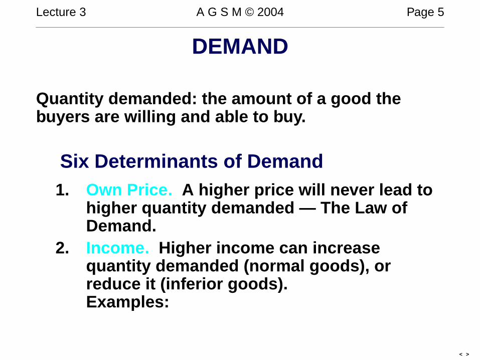
Quantity demanded: the amount of a good thebuyers are willing and able to buy.
Six Determinants of Demand1. Own Price. A higher price will never lead to
higher quantity demanded — The Law ofDemand.
2. Income . Higher income can increasequantity demanded ( normal goods), orreduce it ( inferior goods).Examples:
< >
Lecture 3 A G S M © 2004 Page 6
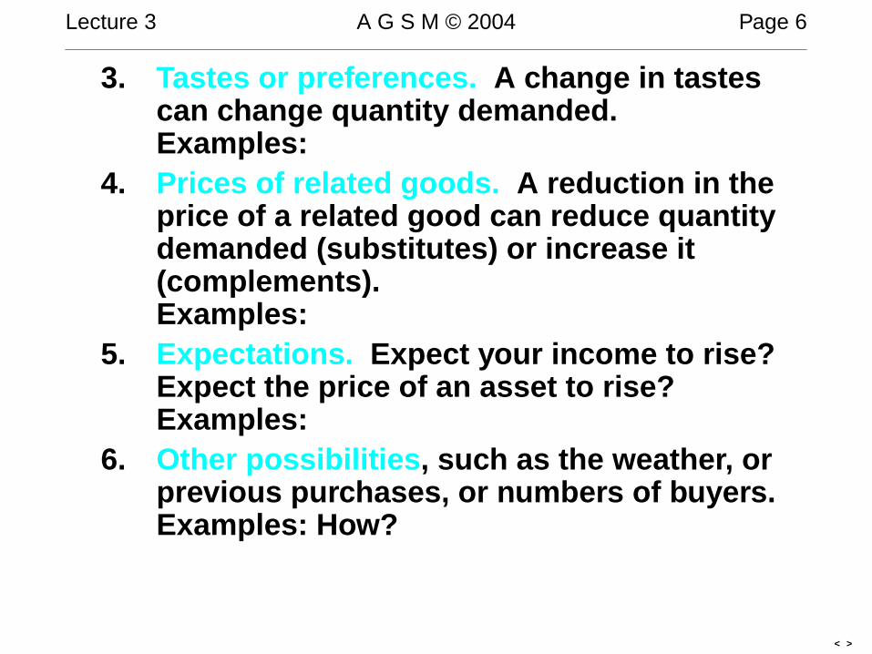
3. Tastes or preferences. A chang e in tastescan chang e quantity demanded.Examples:
4. Prices of related goods. A reduction in theprice of a related good can reduce quantitydemanded ( substitutes) or increase it(complements).Examples:
5. Expectations. Expect your income to rise?Expect the price of an asset to rise?Examples:
6. Other possibilities , such as the weather, orprevious purchases, or numbers of buyers.Examples: How?
< >
Lecture 3 A G S M © 2004 Page 7
CETERIS PARIBUS
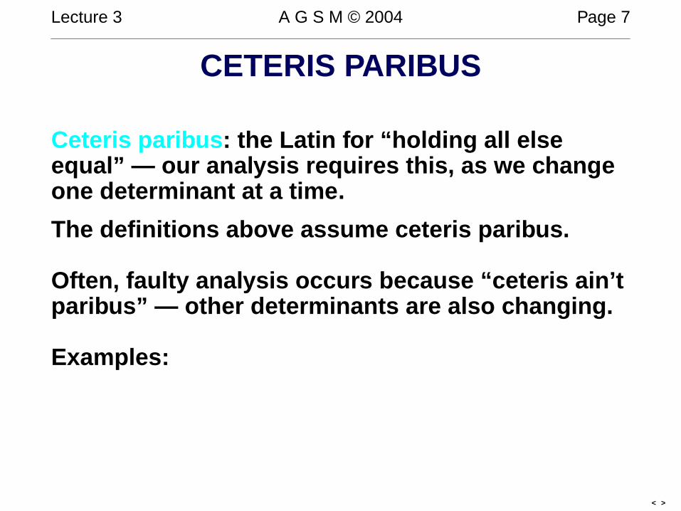
Ceteris paribus : the Latin for “holding all elseequal” — our analysis requires this, as we chang eone determinant at a time.
The definitions above assume ceteris paribus.
Often, faulty analysis occurs because “ceteris ain’tparibus” — other determinants are also changing.
Examples:
< >

Lecture 3 A G S M © 2004 Page 8
INDIVIDUAL DEMANDAssume: individuals want to maximise theirsatisfaction (or utility), subject to the constraints ofprices and income.
Joe has an income of $10/week and spends it all onbananas ($2.99/kg) and oranges (10¢ each).
Model Joe’s preferences for the fruits as a contourof utility (or Indifference Curve): combinations ofthe two goods which give him equal utility.
< >
Lecture 3 A G S M © 2004 Page 9
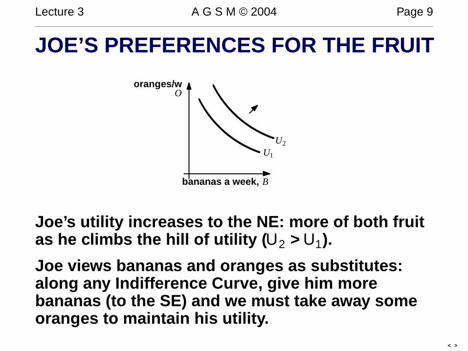
JOE’S PREFERENCES FOR THE FRUIT
bananas a week, B
orang es/wO ............................................................................................................................................................................................................................................................................................................. U1
U2
.............................................................................................................................................................................................................................................................................................................
Joe’s utility increases to the NE: more of both fruitas he climbs the hill of utility ( U2 > U1).
Joe views bananas and oranges as substitutes:along any Indifference Curve , give him morebananas (to the SE) and we must take away someorang es to maintain his utility.
< >
Lecture 3 A G S M © 2004 Page 10
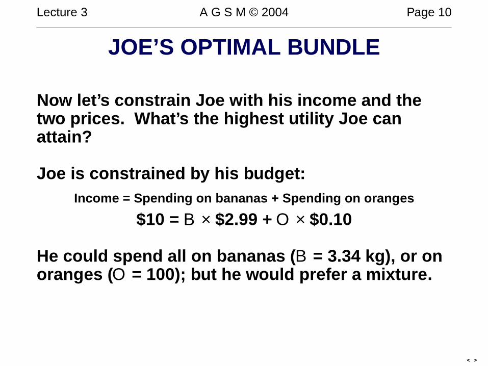
JOE’S OPTIMAL BUNDLE
Now let’s constrain Joe with his income and thetwo prices. What’s the highest utility Joe canattain?
Joe is constrained by his budg et:Income = Spending on bananas + Spending on oranges
$10 = B × $2.99 + O × $0.10
He could spend all on bananas ( B = 3.34 kg), or onorang es (O = 100); but he would prefer a mixture.
< >

Lecture 3 A G S M © 2004 Page 11
GRAPHICAL SOLUTIONPlot the Budget Line:
10 = 2. 99 B + 0. 1O orO = 100 − 29.9 B
to get Joe’s best choice ( B1, O1):
bananas a week, B
orang es/w
O.............................................................................................................................................................................................................................................................................................................
B1
O1
< >

Lecture 3 A G S M © 2004 Page 12
CHANGING DEMANDA frost increases the price of oranges to 13¢ each;the Budget Line rotates down the Orange axis, andJoe is worse off. His optimal bundle chang es.(B2,O2): more bananas, fewer oranges.
bananas a week, B
orang es/wO .............................................................................................................................................................................................................................................................................................................
B1
O1
.............................................................................................................................................................................................................................................................................................................B2
O2
.............................................................................................................................................................................................................................................................................................................
B1
O1
< >

Lecture 3 A G S M © 2004 Page 13
THE DEMAND SCHEDULEShows the relationship between the price of a goodand the maximum quantity demanded per period.(Can also use demand curves and demandfunctions.)
Ice-cream price Quantity demanded by Cate/period$0.00 17
0.50 141.00 101.50 62.00 32.50 13.00 0
Cate always wants more ice-creams (up to satiationat 17/period). At lower prices she can afford more .
< >
Lecture 3 A G S M © 2004 Page 14
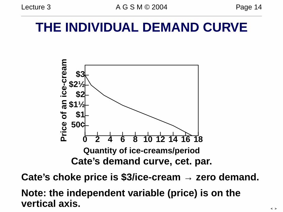
THE INDIVIDUAL DEMAND CURVE
Quantity of ice-creams/period
Pric
e of
an
ice-
crea
m
0 2 4 6 8 10 12 14 16 18
50¢$1
$1½$2
$2½$3
Cate’s demand curve, cet. par.
Cate’s choke price is $3/ice-cream → zero demand.
Note: the independent variable (price) is on thever tical axis.
< >

Lecture 3 A G S M © 2004 Page 15
MARKET DEMANDObtained by horizontally summing individualdemands: at each price , what is the maximum thatCate and Nick demand per period?
Price Cate Nick Market
$0.00 17 + 7 = 240.50 14 6 201.00 10 5 151.50 6 4 102.00 3 3 62.50 1 2 33.00 0 1 1
(There is no reason why the demand curves shouldbe straight lines.)
< >

Lecture 3 A G S M © 2004 Page 16
SHIFTS IN DEMAND
QD
P.........................................................................................................................................................................................................
Distinguish between:• movement along the demand curve as price
chang es, cet. par.
< >

Lecture 3 A G S M © 2004 Page 17
QD
P.........................................................................................................................................................................................................
.........................................................................................................................................................................................................
.........................................................................................................................................................................................................
Distinguish between:• movement along the demand curve as price
chang es, cet. par. and• shifts (contractions ← or expansions →) in
the demand curve as chang es occur in otherdeterminants.
< >

Lecture 3 A G S M © 2004 Page 18
SHIFTS OF THE DEMAND CURVEShifts (contractions ← or expansions →) in thedemand curve as chang es occur in otherdeterminants:— the price of related goods:
expansion : price of “substitute” PY risescontraction : price of “complement” PY rises
— tastes— disposable incomes:
expansion of demand for a normal good whenincome rises or for an inferior good whenincome falls
— expectations of price, availability
< >
Lecture 3 A G S M © 2004 Page 19
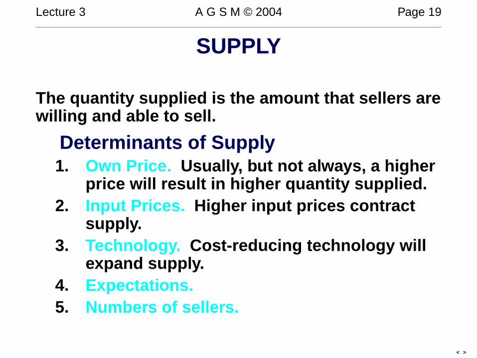
SUPPLY
The quantity supplied is the amount that sellers arewilling and able to sell.
Determinants of Supply1. Own Price. Usually, but not always, a higher
price will result in higher quantity supplied.2. Input Prices. Higher input prices contract
supply.3. Technology. Cost-reducing technology will
expand supply.4. Expectations.5. Numbers of sellers.
< >

Lecture 3 A G S M © 2004 Page 20
THE SUPPLY SCHEDULE— A table that shows the relationship between theprice of a good and the maximum quantitysupplied per period.
Price Quantity supplied/period$0.00 0
0.50 01.00 11.50 22.00 32.50 43.00 5
< >
Lecture 3 A G S M © 2004 Page 21
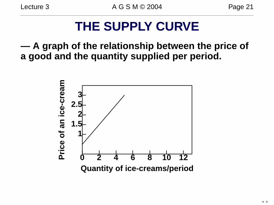
THE SUPPLY CURVE— A graph of the relationship between the price ofa good and the quantity supplied per period.
Quantity of ice-creams/period
Pric
e of
an
ice-
crea
m
0 2 4 6 8 10 12
11.5
22.5
3
< >

Lecture 3 A G S M © 2004 Page 22
MARKET SUPPLYAgain, horizontal sum of the individual supplycur ves:
Price Tony Mick Market$0.00 0 + 0 = 0
0.50 0 0 01.00 1 0 11.50 2 2 42.00 3 4 72.50 4 6 103.00 5 8 13
Although usually upwards sloping (increased priceleads to increased quantity supplied), there is no law ofsupply: supply cur ves can bend backwards.What does a vertical supply cur ve model?
< >

Lecture 3 A G S M © 2004 Page 23
SHIFTS IN THE SUPPLY CURVE
A chang e in the price → a movement along the(unshifting) supply cur ve.
A fall in input prices will shift the curve to the right (atany price , the producer will be prepared to sell more):supply expands.
Ditto an improvement in technology .
And an increase in the number of sellers .
A chang e in expectations can → an expansion insupply ( →) or a contraction in supply ( ←), depending.
< >

Lecture 3 A G S M © 2004 Page 24
SUPPLY & DEMAND
P
Q
D
S..................................................................................................................................................................................................................
................................
...........................
.................................................................................................................
Q*
P*
When S = D , market-clearing equilibrium, at P *, Q*.
< >
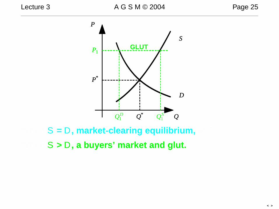
Lecture 3 A G S M © 2004 Page 25
P
Q
D
S..................................................................................................................................................................................................................
................................
...........................
.................................................................................................................
Q*
P*
P1
QD1 QS
1
GLUT
When S = D , market-clearing equilibrium, at P *, Q*.
When S > D , a buyers’ market and glut.
< >

Lecture 3 A G S M © 2004 Page 26
P
Q
D
S..................................................................................................................................................................................................................
................................
...........................
.................................................................................................................
Q*
P*
P2
QS2 QD
2
SHORTA GE
When S = D , market-clearing equilibrium , at P *, Q*.
When D > S , a sellers’ market and shortage .
< >

Lecture 3 A G S M © 2004 Page 27
P
Q
D
S..................................................................................................................................................................................................................
................................
...........................
.................................................................................................................
Q*
P*
P1GLUT
QD1 QS
1
P2SHORTA GE
QS2 QD
2
When S = D , market-clearing equilibrium , at P *, Q*.
When S > D , a buyers’ market and glut.
When D > S , a sellers’ market and shortage .
< >
Lecture 3 A G S M © 2004 Page 28
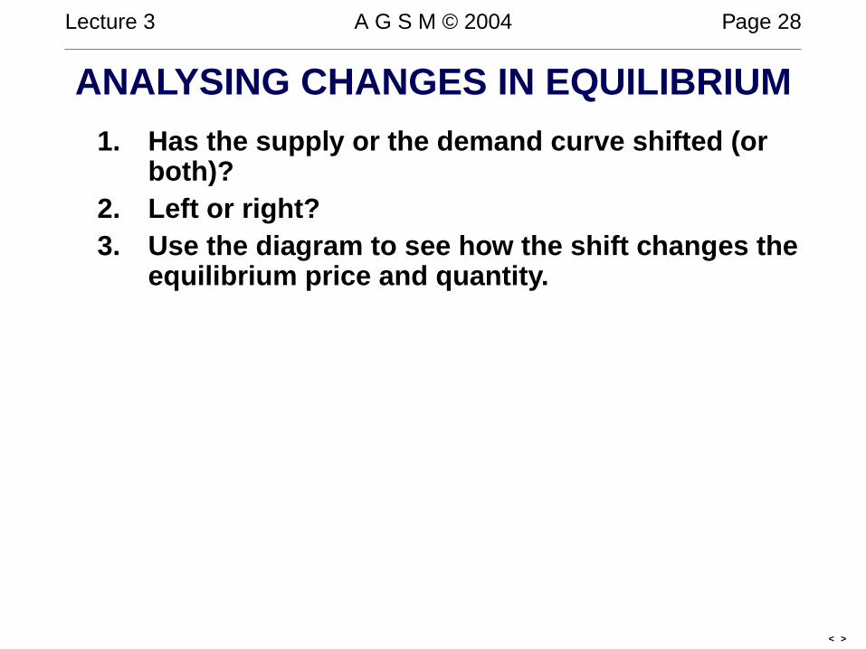
ANALYSING CHANGES IN EQUILIBRIUM
1. Has the supply or the demand curve shifted (orboth)?
2. Left or right?3. Use the diagram to see how the shift chang es the
equilibrium price and quantity.
< >

Lecture 3 A G S M © 2004 Page 29
ILLICIT-DRUG POLICIES
Supply-side policy targets the drug pushers and theupstream suppliers. Demand-side policy attempts torehabilitate or to deter drug users. How to they differ inour analysis?
Supply-side policies have the effect of reducing theamount of drugs on offer at any price: the supply cur vecontracts to the left. Prices rise.
Demand-side policies have the effect of reducing thequantity of drugs demanded at any price: the demandcur ve contracts to the left. Prices fall.
If there is a mixture of both policies, then both curvescontract to the left: prices may rise or fall, dependingon the relative shifts.
< >

Lecture 3 A G S M © 2004 Page 30
MODELLING THE BLACK MARKET
P
Q
D
S..................................................................................................................................................................................................................
................................
...........................
.................................................................................................................
Q*
P*
....................................
.............................
..............................................................................................................................S′...............................................................................................................................................................................................
D′
The green contracted supply cur ve S ′ models supply-side policy: equilibrium quantity is reduced but price isup. The red contracted demand curve D ′ modelsdemand-side policy: both equilibrium quantity andprice are reduced.
<