lecture 26 constrained nonlinear problems …angelia/ge330fall09_nlpkkt_l26.pdflecture 26...

Lecture 26

Constrained Nonlinear Problems

Necessary KKT Optimality Conditions

November 18, 2009

Lecture 26

Outline

• Necessary Optimality Conditions for Constrained Problems

• Karush-Kuhn-Tucker∗ (KKT) optimality conditions

� Equality constrained problems

� Inequality and equality constrained problems

• Convex Inequality Constrained Problems

� Sufficient optimality conditions

• The material is in Chapter 18 of the book

• Section 18.1.1

• Lagrangian Method in Section 18.2 (see 18.2.1 and 18.2.2)

∗William Karush develop these conditions in 1939 as a part of his M.S. thesis at the University of Chicago; the same weredeveloped independently later in 1951 by Harold W. Kuhn and Albert W. Tucker.

Operations Research Methods 1

Lecture 26

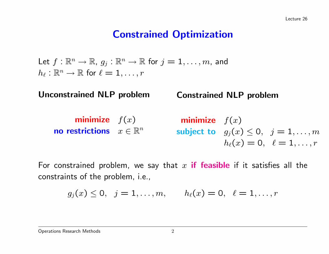
Constrained Optimization

Let f : Rn → R, gj : Rn → R for j = 1, . . . , m, and

h` : Rn → R for ` = 1, . . . , r

Unconstrained NLP problem

minimize f(x)

no restrictions x ∈ Rn

Constrained NLP problem

minimize f(x)

subject to gj(x) ≤ 0, j = 1, . . . , m

h`(x) = 0, ` = 1, . . . , r

For constrained problem, we say that x if feasible if it satisfies all the

constraints of the problem, i.e.,

gj(x) ≤ 0, j = 1, . . . , m, h`(x) = 0, ` = 1, . . . , r


Lecture 26

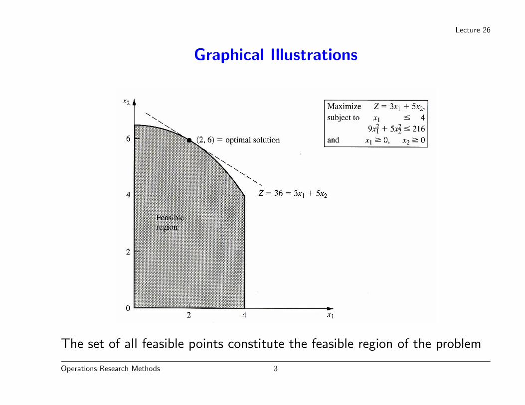
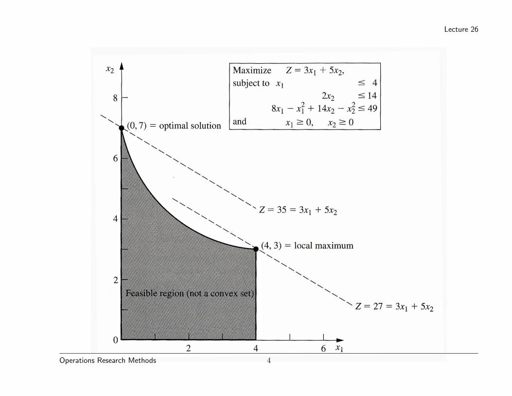
Graphical Illustrations

The set of all feasible points constitute the feasible region of the problem


Lecture 26


Lecture 26

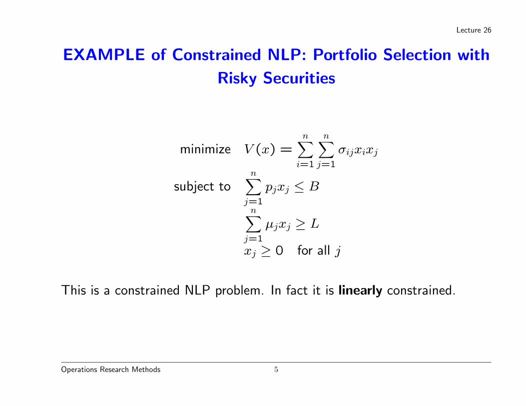
EXAMPLE of Constrained NLP: Portfolio Selection with

Risky Securities

minimize V (x) =n∑

i=1

n∑j=1

σijxixj

subject ton∑

j=1

pjxj ≤ B

n∑j=1

µjxj ≥ L

xj ≥ 0 for all j

This is a constrained NLP problem. In fact it is linearly constrained.


Lecture 26

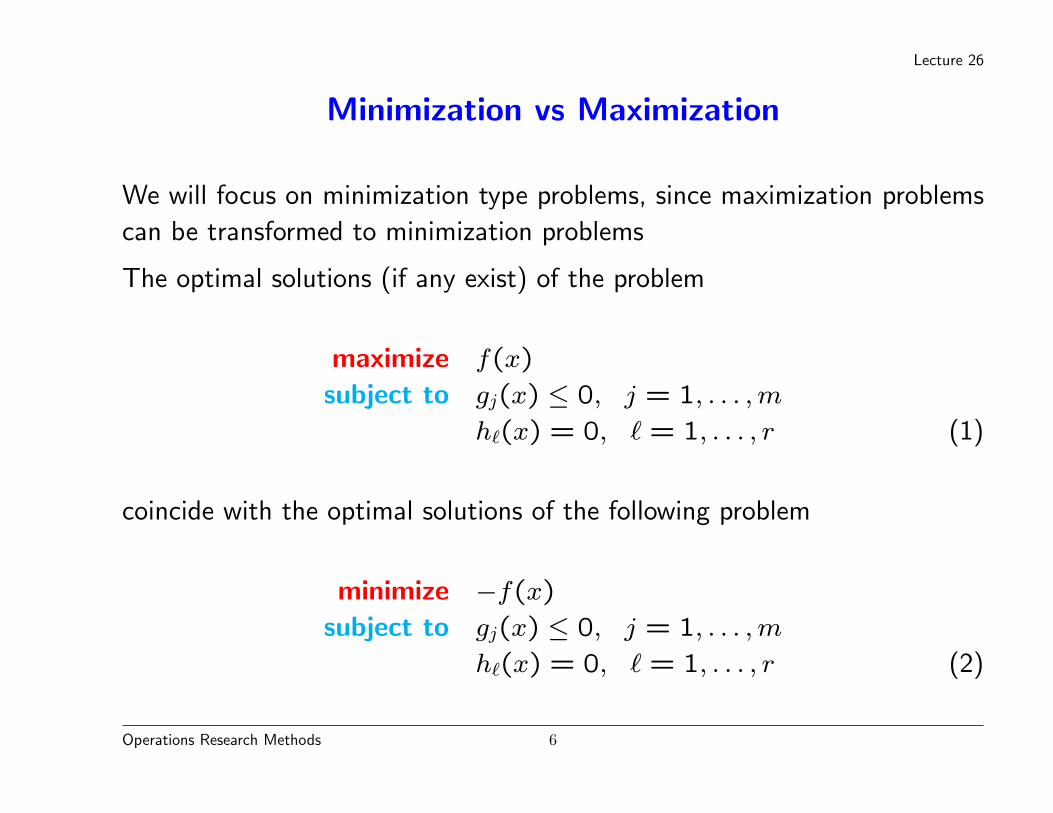
Minimization vs Maximization

We will focus on minimization type problems, since maximization problems

can be transformed to minimization problems

The optimal solutions (if any exist) of the problem

maximize f(x)

subject to gj(x) ≤ 0, j = 1, . . . , m

h`(x) = 0, ` = 1, . . . , r (1)

coincide with the optimal solutions of the following problem

minimize −f(x)

subject to gj(x) ≤ 0, j = 1, . . . , m

h`(x) = 0, ` = 1, . . . , r (2)


Lecture 26

NOTE: The optimal values of the problems (1) and (2) are obviously not

the same (differ in sign)

Furthermore, the local maxima of problem (1) coincide with the local

minima of problem (2).


Lecture 26

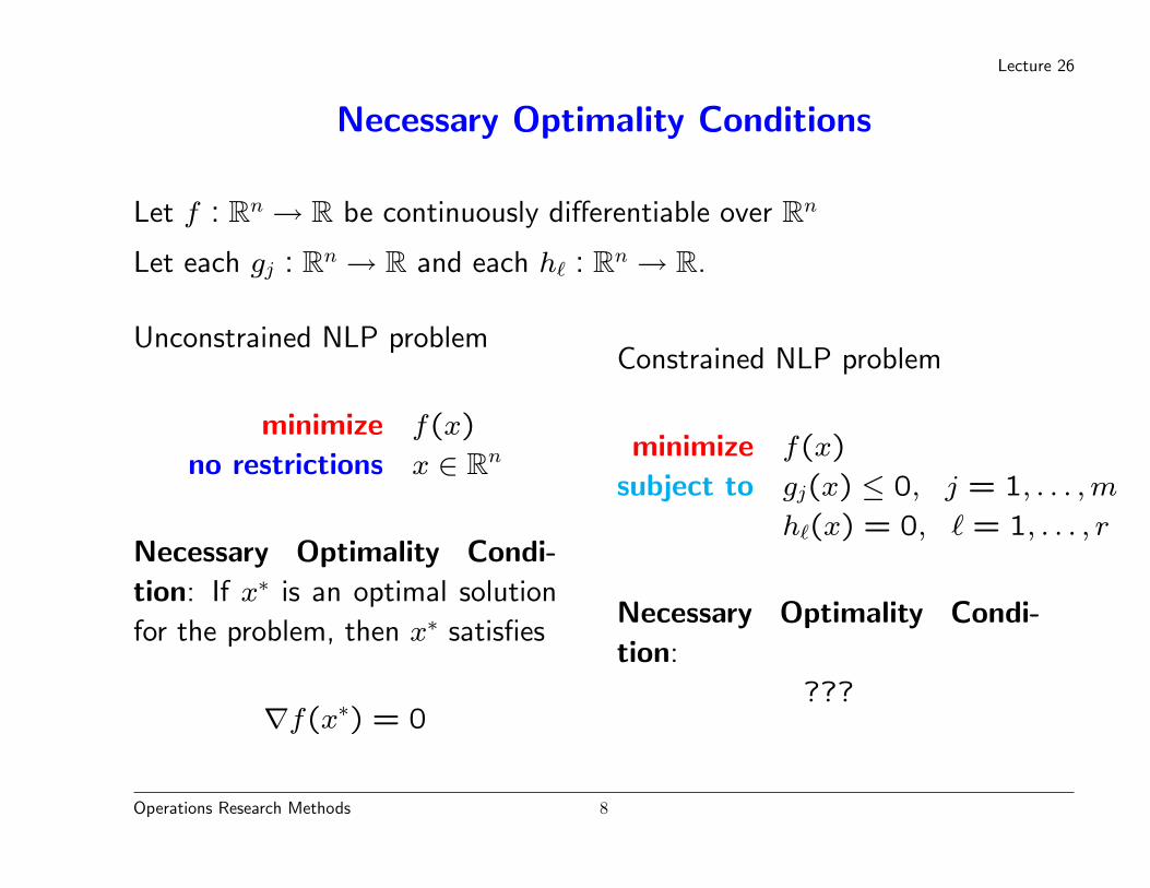
Necessary Optimality Conditions

Let f : Rn → R be continuously differentiable over Rn

Let each gj : Rn → R and each h` : Rn → R.

Unconstrained NLP problem

minimize f(x)

no restrictions x ∈ Rn

Necessary Optimality Condi-

tion: If x∗ is an optimal solution

for the problem, then x∗ satisfies

∇f(x∗) = 0

Constrained NLP problem

minimize f(x)

subject to gj(x) ≤ 0, j = 1, . . . , m

h`(x) = 0, ` = 1, . . . , r

Necessary Optimality Condi-

tion:

???


Lecture 26

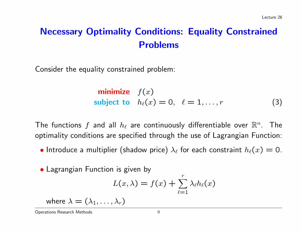
Necessary Optimality Conditions: Equality Constrained

Problems

Consider the equality constrained problem:

minimize f(x)

subject to h`(x) = 0, ` = 1, . . . , r (3)

The functions f and all h` are continuously differentiable over Rn. The

optimality conditions are specified through the use of Lagrangian Function:

• Introduce a multiplier (shadow price) λ` for each constraint h`(x) = 0.

• Lagrangian Function is given by

L(x, λ) = f(x) +r∑

`=1

λ`h`(x)

where λ = (λ1, . . . , λr)Operations Research Methods 9

Lecture 26

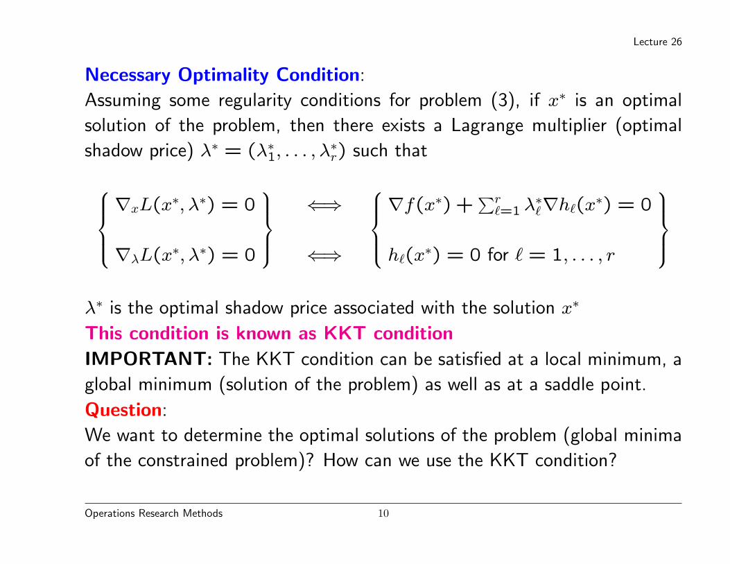
Necessary Optimality Condition:

Assuming some regularity conditions for problem (3), if x∗ is an optimal

solution of the problem, then there exists a Lagrange multiplier (optimal

shadow price) λ∗ = (λ∗1, . . . , λ∗r) such that

∇xL(x∗, λ∗) = 0

∇λL(x∗, λ∗) = 0

⇐⇒

⇐⇒

∇f(x∗) +

∑r`=1 λ∗`∇h`(x∗) = 0

h`(x∗) = 0 for ` = 1, . . . , r

λ∗ is the optimal shadow price associated with the solution x∗

This condition is known as KKT condition

IMPORTANT: The KKT condition can be satisfied at a local minimum, a

global minimum (solution of the problem) as well as at a saddle point.

Question:

We want to determine the optimal solutions of the problem (global minima

of the constrained problem)? How can we use the KKT condition?


Lecture 26

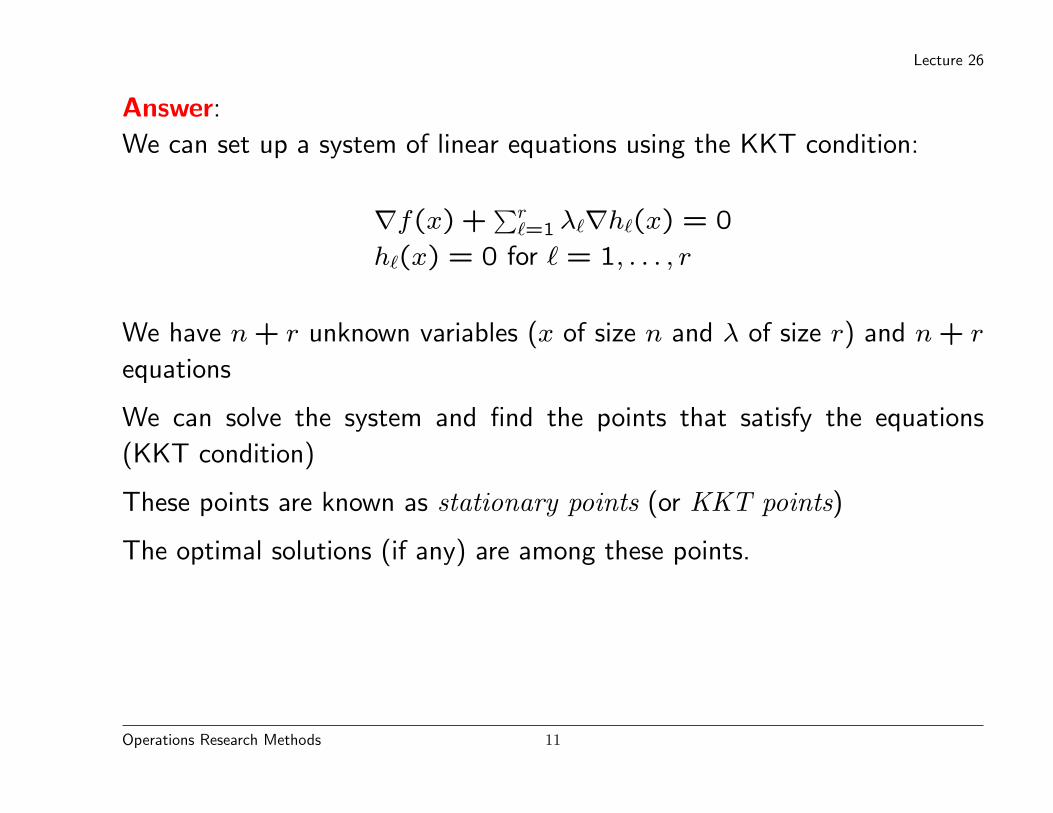
Answer:

We can set up a system of linear equations using the KKT condition:

∇f(x) +∑r

`=1 λ`∇h`(x) = 0

h`(x) = 0 for ` = 1, . . . , r

We have n + r unknown variables (x of size n and λ of size r) and n + r

equations

We can solve the system and find the points that satisfy the equations

(KKT condition)

These points are known as stationary points (or KKT points)

The optimal solutions (if any) are among these points.


Lecture 26

NOTE:

We need additional information to characterize the stationary points as

global or local minimum or other by using the second order information for

the objective f(x) at the KKT points (see Lecture 25).


Lecture 26

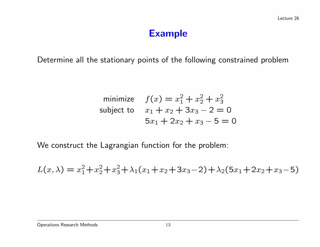
Example

Determine all the stationary points of the following constrained problem

minimize f(x) = x21 + x2

2 + x23

subject to x1 + x2 + 3x3 − 2 = 0

5x1 + 2x2 + x3 − 5 = 0

We construct the Lagrangian function for the problem:

L(x, λ) = x21+x2

2+x23+λ1(x1+x2+3x3−2)+λ2(5x1+2x2+x3−5)


Lecture 26

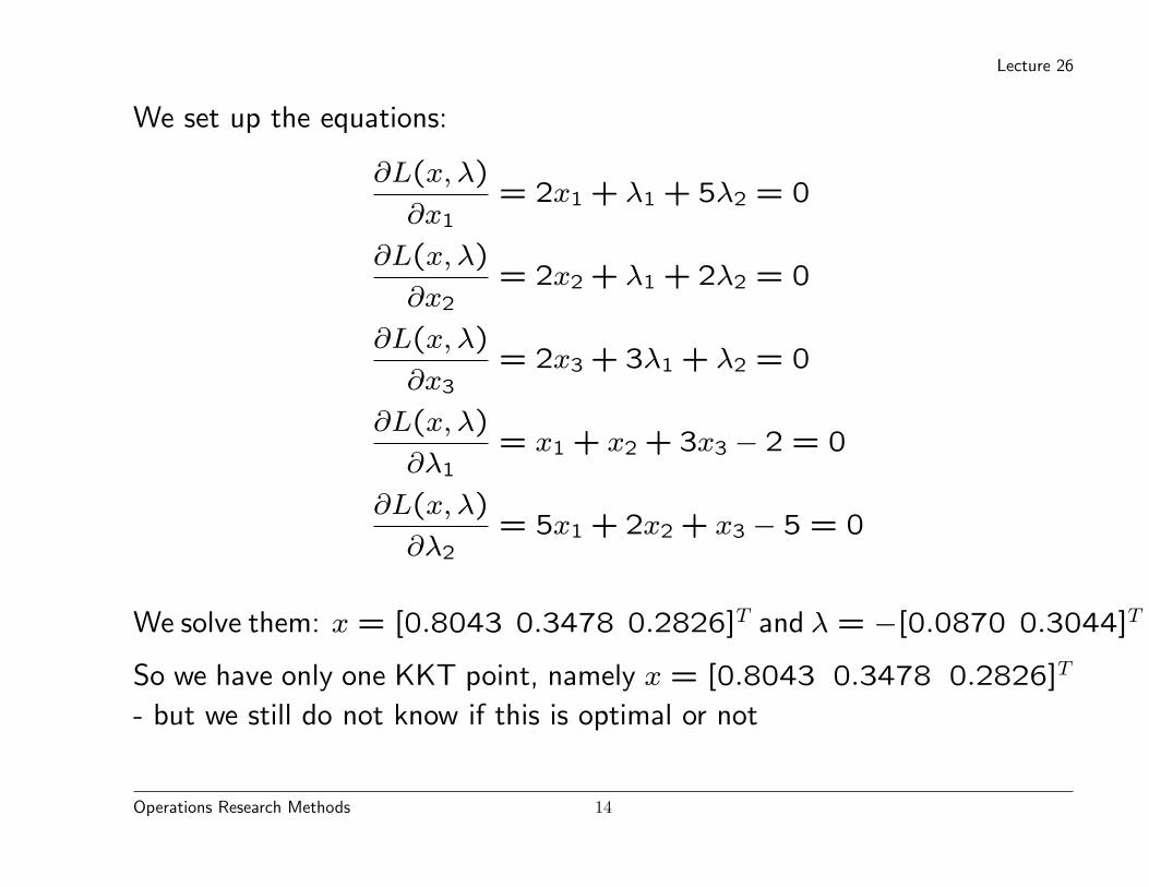
We set up the equations:

∂L(x, λ)

∂x1= 2x1 + λ1 + 5λ2 = 0

∂L(x, λ)

∂x2= 2x2 + λ1 + 2λ2 = 0

∂L(x, λ)

∂x3= 2x3 + 3λ1 + λ2 = 0

∂L(x, λ)

∂λ1= x1 + x2 + 3x3 − 2 = 0

∂L(x, λ)

∂λ2= 5x1 + 2x2 + x3 − 5 = 0

We solve them: x = [0.8043 0.3478 0.2826]T and λ = −[0.0870 0.3044]T

So we have only one KKT point, namely x = [0.8043 0.3478 0.2826]T

- but we still do not know if this is optimal or not


Lecture 26

We can check the Hessian of f . We will find that the Hessian is given by a

diagonal matrix with diagonal entries equal to 2.

The Hessian is positive definite, therefore the point x∗ is a global minimum.


Lecture 26

Necessary Optimality Conditions: Inequality and Equality

Constrained Problems

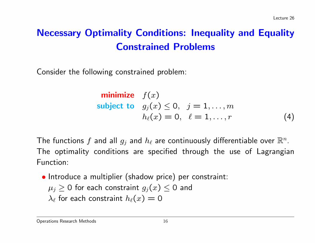
Consider the following constrained problem:

minimize f(x)

subject to gj(x) ≤ 0, j = 1, . . . , m

h`(x) = 0, ` = 1, . . . , r (4)

The functions f and all gj and h` are continuously differentiable over Rn.

The optimality conditions are specified through the use of Lagrangian

Function:

• Introduce a multiplier (shadow price) per constraint:

µj ≥ 0 for each constraint gj(x) ≤ 0 and

λ` for each constraint h`(x) = 0


Lecture 26

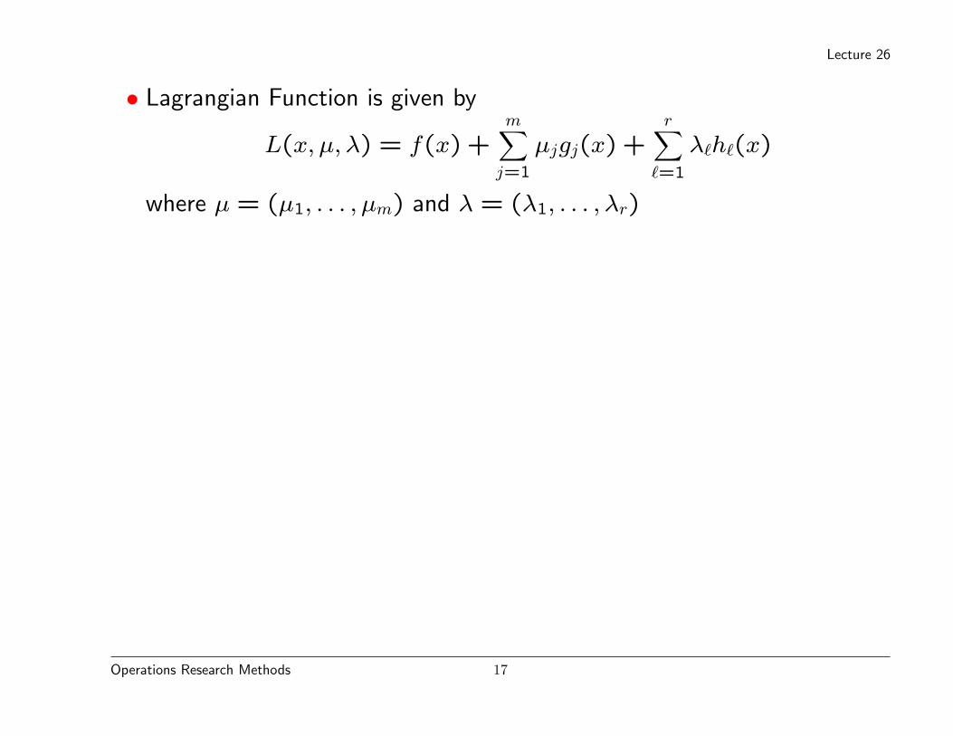
• Lagrangian Function is given by

L(x, µ, λ) = f(x) +m∑

j=1

µjgj(x) +r∑

`=1

λ`h`(x)

where µ = (µ1, . . . , µm) and λ = (λ1, . . . , λr)


Lecture 26

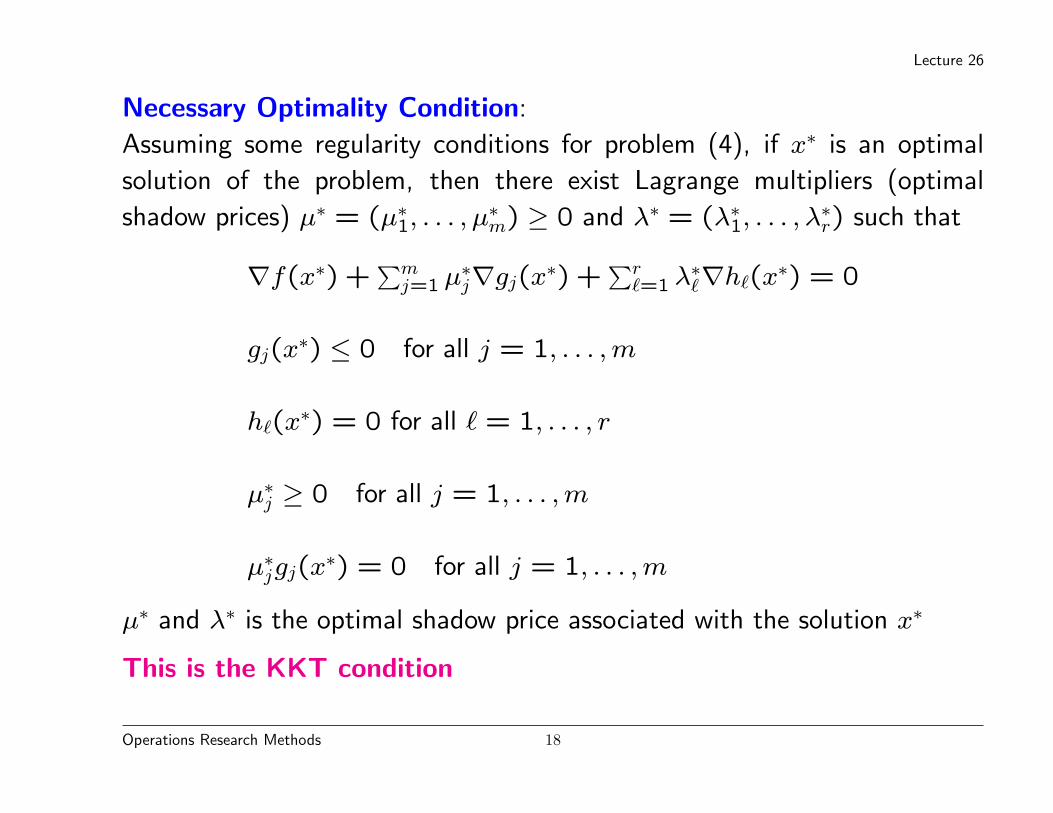
Necessary Optimality Condition:

Assuming some regularity conditions for problem (4), if x∗ is an optimal

solution of the problem, then there exist Lagrange multipliers (optimal

shadow prices) µ∗ = (µ∗1, . . . , µ∗m) ≥ 0 and λ∗ = (λ∗1, . . . , λ

∗r) such that

∇f(x∗) +∑m

j=1 µ∗j∇gj(x∗) +∑r

`=1 λ∗`∇h`(x∗) = 0

gj(x∗) ≤ 0 for all j = 1, . . . , m

h`(x∗) = 0 for all ` = 1, . . . , r

µ∗j ≥ 0 for all j = 1, . . . , m

µ∗jgj(x∗) = 0 for all j = 1, . . . , m

µ∗ and λ∗ is the optimal shadow price associated with the solution x∗

This is the KKT condition


Lecture 26

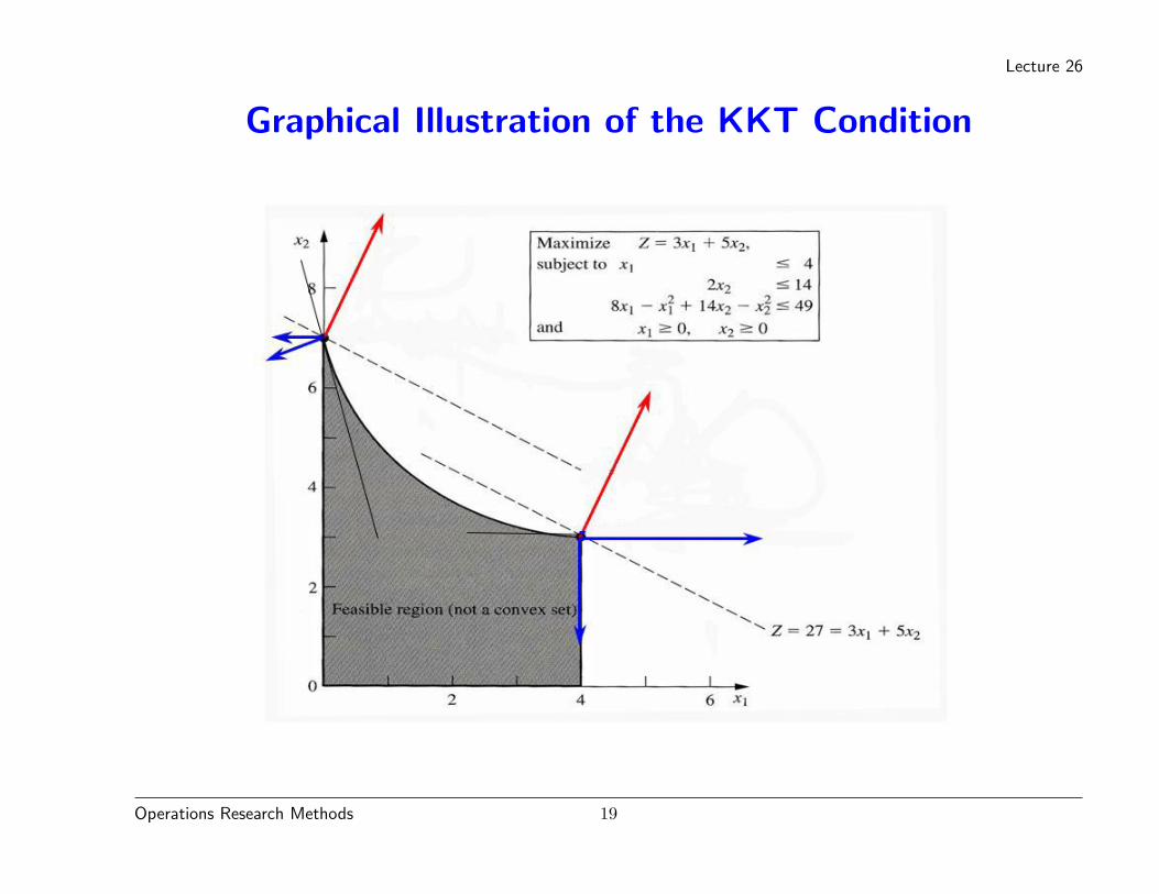
Graphical Illustration of the KKT Condition


Lecture 26

IMPORTANT: The KKT condition can be satisfied at a local minimum, a

global minimum (solution of the problem) as well as at a saddle point.

We can use the KKT condition to characterize all the stationary points

of the problem, and then perform some additional testing to determine

the optimal solutions of the problem (global minima of the constrained

problem).


Lecture 26

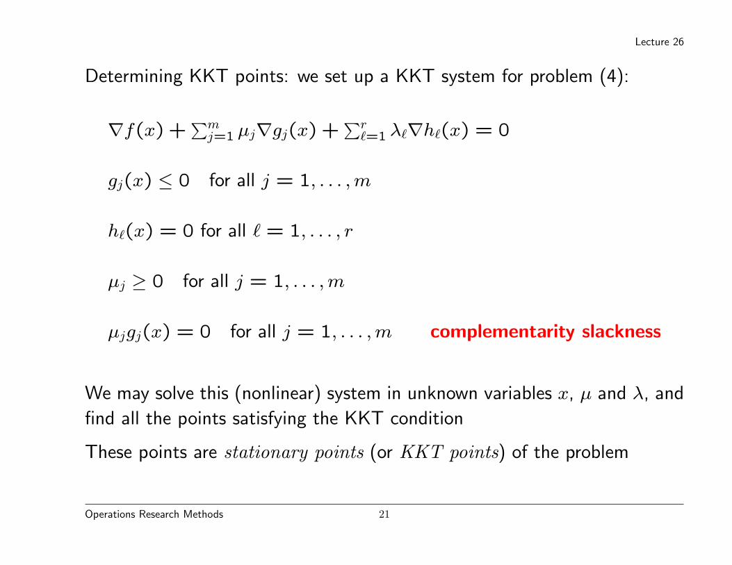
Determining KKT points: we set up a KKT system for problem (4):

∇f(x) +∑m

j=1 µj∇gj(x) +∑r

`=1 λ`∇h`(x) = 0

gj(x) ≤ 0 for all j = 1, . . . , m

h`(x) = 0 for all ` = 1, . . . , r

µj ≥ 0 for all j = 1, . . . , m

µjgj(x) = 0 for all j = 1, . . . , m complementarity slackness

We may solve this (nonlinear) system in unknown variables x, µ and λ, and

find all the points satisfying the KKT condition

These points are stationary points (or KKT points) of the problem


Lecture 26

The optimal points are among the KKT points

We need additional information to characterize the KKT points as global or

local minimum or other - we use the second order information, as discussed

in Lecture 25.


Lecture 26

Sufficient Optimality Conditions: Convex Inequality

Constrained Problems

Consider the following constrained problem:

minimize f(x)

subject to gj(x) ≤ 0, j = 1, . . . , m (5)

Functions f and all gj are convex and continuously differentiable over Rn.

We say that the problem is convex For this convex problem, the KKT

conditions are also sufficient for optimality.


Lecture 26

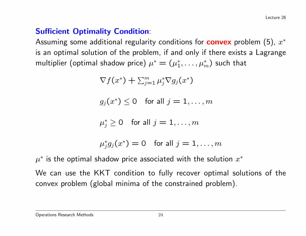
Sufficient Optimality Condition:

Assuming some additional regularity conditions for convex problem (5), x∗

is an optimal solution of the problem, if and only if there exists a Lagrange

multiplier (optimal shadow price) µ∗ = (µ∗1, . . . , µ∗m) such that

∇f(x∗) +∑m

j=1 µ∗j∇gj(x∗)

gj(x∗) ≤ 0 for all j = 1, . . . , m

µ∗j ≥ 0 for all j = 1, . . . , m

µ∗jgj(x∗) = 0 for all j = 1, . . . , m

µ∗ is the optimal shadow price associated with the solution x∗

We can use the KKT condition to fully recover optimal solutions of the

convex problem (global minima of the constrained problem).


Lecture 26

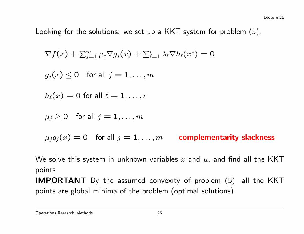
Looking for the solutions: we set up a KKT system for problem (5),

∇f(x) +∑m

j=1 µj∇gj(x) +∑r

`=1 λ`∇h`(x∗) = 0

gj(x) ≤ 0 for all j = 1, . . . , m

h`(x) = 0 for all ` = 1, . . . , r

µj ≥ 0 for all j = 1, . . . , m

µjgj(x) = 0 for all j = 1, . . . , m complementarity slackness

We solve this system in unknown variables x and µ, and find all the KKT

points

IMPORTANT By the assumed convexity of problem (5), all the KKT

points are global minima of the problem (optimal solutions).


Lecture 26

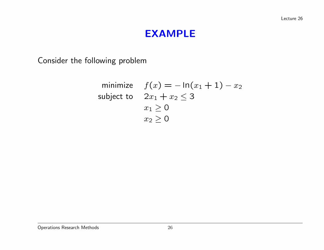
EXAMPLE

Consider the following problem

minimize f(x) = − ln(x1 + 1)− x2

subject to 2x1 + x2 ≤ 3

x1 ≥ 0

x2 ≥ 0


lecture 26 constrained nonlinear problems …angelia/ge330fall09_nlpkkt_l26.pdflecture 26...

Documents