UNLV Theses, Dissertations, Professional Papers, and Capstones

5-2009

Turn Constrained Path Planning Problems Turn Constrained Path Planning Problems

Victor M. Roman University of Nevada, Las Vegas

Follow this and additional works at: https://digitalscholarship.unlv.edu/thesesdissertations

Part of the Navigation, Guidance, Control and Dynamics Commons, Other Computer Sciences

Commons, and the Theory and Algorithms Commons

Repository Citation Repository Citation Roman, Victor M., "Turn Constrained Path Planning Problems" (2009). UNLV Theses, Dissertations, Professional Papers, and Capstones. 1202. http://dx.doi.org/10.34917/2754351

This Thesis is protected by copyright and/or related rights. It has been brought to you by Digital Scholarship@UNLV with permission from the rights-holder(s). You are free to use this Thesis in any way that is permitted by the copyright and related rights legislation that applies to your use. For other uses you need to obtain permission from the rights-holder(s) directly, unless additional rights are indicated by a Creative Commons license in the record and/or on the work itself. This Thesis has been accepted for inclusion in UNLV Theses, Dissertations, Professional Papers, and Capstones by an authorized administrator of Digital Scholarship@UNLV. For more information, please contact digitalscholarship@unlv.edu.

TURN CONSTRAINED PATH PLANNING PROBLEMS

by

Victor M. Roman

Bachelors of Science in Electronic Engineering Northrop University

1984

Bachelor of Science in Computer Science University of Nevada, Las Vegas

2006

A thesis submitted in partial fulfillment of the requirement for the

Master of Science Degree in Computer Science Computer Science Department

School of Computer Science

Graduate College University of Nevada, Las Vegas

May 2009

UMI Number: 1472438

INFORMATION TO USERS

The quality of this reproduction is dependent upon the quality of the copy

submitted. Broken or indistinct print, colored or poor quality illustrations

and photographs, print bleed-through, substandard margins, and improper

alignment can adversely affect reproduction.

In the unlikely event that the author did not send a complete manuscript

and there are missing pages, these will be noted. Also, if unauthorized

copyright material had to be removed, a note will indicate the deletion.

®

UMI UMI Microform 1472438

Copyright 2009 by ProQuest LLC All rights reserved. This microform edition is protected against

unauthorized copying under Title 17, United States Code.

ProQuest LLC 789 East Eisenhower Parkway

P.O. Box 1346 Ann Arbor, Ml 48106-1346

\B~J X i j JSL~J. &51I

Thesis Approval The Graduate College University of Nevada, Las Vegas

APRIL 13TH .20 09

The Thesis prepared by

VICTOR M. ROMAN

Entitled

TURN CONSTRAINED PATH PLANNING PROBLEMS

is approved in partial fulfillment of the requirements for the degree of

MASTER OF SCIENCE IN COMPUTER SCIENCE

Examination Committee Chair

Dean of the Graduate College

Examination Committee Member

Examination Committee Member

GraAuateCollege Faculty Representative

1017-53 11

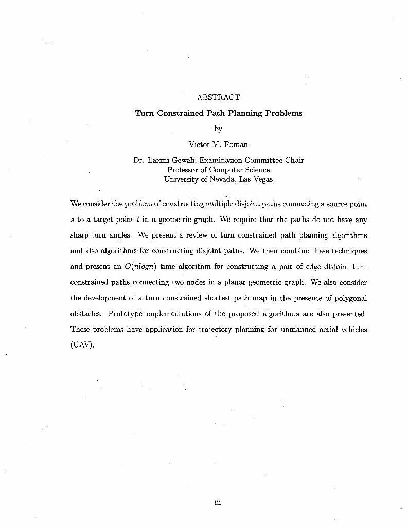
ABSTRACT

Turn Constrained Path Planning Problems

by

Victor M. Roman

Dr. Laxmi Gewali, Examination Committee Chair Professor of Computer Science

University of Nevada, Las Vegas

We consider the problem of constructing multiple disjoint paths connecting a source point

s to a target point t in a geometric graph. We require that the paths do not have any

sharp turn angles. We present a review of turn constrained path planning algorithms

and also algorithms for constructing disjoint paths. We then combine these techniques

and present an 0(nlogn) time algorithm for constructing a pair of edge disjoint turn

constrained paths connecting two nodes in a planar geometric graph. We also consider

the development of a turn constrained shortest path map in the presence of polygonal

obstacles. Prototype implementations of the proposed algorithms are also presented.

These problems have application for trajectory planning for unmanned aerial vehicles

(UAV).

in

TABLE OF CONTENTS

ABSTRACT iii

LIST OF FIGURES . . vi

LIST OF TABLES viii

ACKNOWLEDGMENTS ix

CHAPTER 1 INTRODUCTION 1

CHAPTER 2 TURN CONSTRAINED DISJOINT PATHS 3

2.1 Turn Constrained Shortest Path 3

2.2 Shortest Disjoint Path Pairs 5

2.3 Constrained Disjoint Path Pairs 8

CHAPTER 3 CONSTRAINT SHORTEST PATH MAP (CSPM) 13

3.1 Shortest Path Map 13

3.2 Constrained Shortest Path Map 22

3.3 Extending CSPM to add partially forbidden region 25

CHAPTER 4 IMPLEMENTATION 27

4.1 Turn Constrained Disjoint Path Interface 27

4.1.1 Interface Description 27

4.1.2 Icon Functionality Description 28

4.1.3 Program menu items 29

4.1.4 Visibility Edge Generation 30

4.1.5 Constrained Path Generation 31

4.2 Constrained Shortest Path Map Interface 31

4.2.1 Interface Description 32

4.2.2 Icon Functionality Description 34

iv

4.2.3 Program Submenu Description 36

4.2.4 SPM Implementation 38

CHAPTER 5 CONCLUSION 41

BIBLIOGRAPHY . 43

VITA 45

v

LIST OF FIGURES

Figure 2.1 Transform G to G' 4

Figure 2.2 Example Path Types 5

Figure 2.3 Shortest Path from 5 to t 6

Figure 2.4 Tagging of Shortest Path 7

Figure 2.5 Disjoint Path Pair 7

Figure 2.6 Cut Path 8

Figure 2.7 Constrained Path PI 9

Figure 2.8 Tagging of Constrained Path PI 9

Figure 2.9 Constrained Disjoint Path Pair PI and P2 10

Figure 3.1 SPM Graph (Single obstacle) 13

Figure 3.2 Bisector 14

Figure 3.3 SPM Graph (two obstacles) 16

Figure 3.4 SPM for many obstacles 17

Figure 3.5 s Vertex Free Region 18

Figure 3.6 s Vertex Free region with Bisector 19

Figure 3.7 Vi Generated Free Region 20

Figure 3.8 Illustrating Restricted Faces and Forbidden regions 23

Figure 3.9 Final CSPM 26

Figure 4.1 Constraint GUI Layout 28

Figure 4.2 Constraint Program Main 28

Figure 4.3 Program Options 30

Figure 4.4 Visibility Edges 31

Figure 4.5 Constrained Paths 32

vi

Figure 4.6 Planar GUI Layout 33

Figure 4.7 Partition GUI Layout 33

Figure 4.8 Planar Program Main GUI 34

Figure 4.9 Planar Program Partition GUI 35

Figure 4.10 Planar Program File Options 37

Figure 4.11 Planar Program Partition options 38

Figure 4.12 Graph G Before Partition 39

Figure 4.13 Graph G Partitioned into regions 40

Figure 4.14 Shortest Path from s to t • • • • 40

vn

LIST OF TABLES

Table 4.1 Icon description 29

Table 4.2 File menu Items description 29

Table 4.3 Options menu Items description 30

Table 4.4 Icon description 35

Table 4.5 Icon description continued 36

Table 4.6 File menu Items description 36

Table 4.7 Options and Help menu Items description 36

Table 4.8 File and Options menu Items description 37

vm

ACKNOWLEDGMENTS

I would like to thank my advisor, Dr. Laxmi Gewali, for his support and guidance

during the course of my graduate studies. Dr. Gewali was always available and was

extremely generous with his time.

Additional thanks to Professor Lee Mish who believed in me when I first decided to

start graduate school, to Dr. Jan Pedersen whom would recognize the influence of his

programming style in the implementation phase of this project, as well as Dr. Ajoy K

Datta, Dr. John Minor, and Dr. Yoowan Kim.

Finally, I would like to thank my father for his unwavering support and encouragement

throughout my years of study.

IX

CHAPTER 1

INTRODUCTION

The problem of computing shortest path in a weighted network has attracted the inter­

est of many researchers and several efficient algorithms to solve this problem have been

reported [3, 10]. In a two dimensional Euclidian plane that contains obstacles, the ap­

plication of shortest path is used to determine a collision free path connecting two given

points. Note that a path that traverses only the free-space is called a collision-free path.

One of the approaches for finding the shortest collision-free path in 2-dimensions is to

convert the problem into an equivalent problem in a geometric graph. Specifically, the

collection of obstacles in 2-dimensions is converted into a graph called the visibility graph

[10]. It has been formally established that the shortest collision-free path can be com­

puted by finding the shortest path in the visibility graph. The main reason behind this

fact is that if a shortest path touches the obstacle, then it must touch in one of the ver­

tices. Several variations of shortest-path computations have been considered. One such

variation is to find a path connecting two given vertices with a minimum number of link

hops. Such a path is called a link minimized path and efficient algorithms for computing

such path are reported in [9]. Another variation of shortest-path problem is obtained by

imposing turn angle constraint. Specifically, it is required to construct a shortest path in

the presence of obstacles such that the turn implied by consecutive segments in the path

is no more than a given value. One of the algorithms for computing the turn constrain

shortest path in two dimensions was reported by Borujerdi and Uhlmann in [1].

Several researchers have also considered the problem of computing more than one

short length path connecting two vertices in a network. One of the early results on

computing a pair of node disjoint paths connecting two given vertices in a network was

1

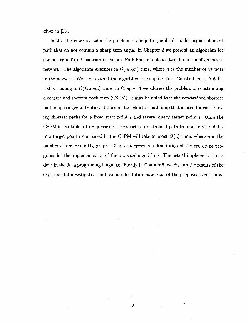
given in [13].

In this thesis we consider the problem of computing multiple node disjoint shortest

path that do not contain a sharp turn angle. In Chapter 2 we present an algorithm for

computing a Turn Constrained Disjoint Path Pair in a planar two dimensional geometric

network. The algorithm executes in 0(nlogn) time, where n is the number of vertices

in the network. We then extend the algorithm to compute Turn Constrained k-Disjoint

Paths running in 0(knlogn) time. In Chapter 3 we address the problem of constructing

a constrained shortest path map (CSPM). It may be noted that the constrained shortest

path map is a generalization of the standard shortest path map that is used for construct­

ing shortest paths for a fixed start point s and several query target point t. Once the

CSPM is available future queries for the shortest constrained path from a source point s

to a target point t contained in the CSPM will take at most 0(n) time, where n is the

number of vertices in the graph. Chapter 4 presents a description of the prototype pro­

grams for the implementation of the proposed algorithms. The actual implementation is

done in the Java programing language. Finally in Chapter 5, we discuss the results of the

experimental investigation and avenues for future extension of the proposed algorithms.

2

CHAPTER 2

TURN CONSTRAINED DISJOINT PATHS

2.1 Turn Constrained Shortest Path

In this chapter we consider the problem of planning multiple disjoint short length paths

connecting a source point s to a target point t in a 2-D geometric graph such that the

path has no turn angle more than a given value.

Finding a shortest path connecting two vertices in a graph is a well explored problem

and several algorithms for obtaining the solution have been reported [3, 4]. A path

extracted from a geometric graph consists of a sequence of line segments. Two consecutive

line segments in the path define the turn angle between them. In many applications, a

path with a sharp turn angle may not be acceptable. For example, sharp turn paths can

not be used by aerial vehicles. In fact most aerial vehicles can not make a turn of more

than 30° [6]. While a variety of algorithms have been developed for constructing shortest

path [3, 4], only a few algorithms have been reported addressing the turn constraint

property. One of the important algorithmic results on turn constrained shortest path

was developed by Boroujerdi and Uhlmann [1]. The algorithm reported in their paper

[1] uses a graph transformation technique to solve the turn constrained shortest path

problem in a 0(|£7|Zop|Vj) time. Their technique is to transform a given graph G into

G" such that the shortest path in G' corresponds to a turn constrained shortest path in

G. An overview of this technique can be briefly described as follows.

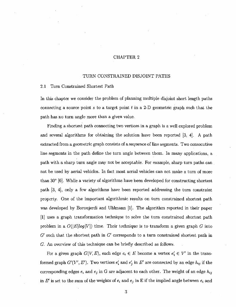
For a given graph G(V, E), each edge e* G E become a vertex e't G V in the trans­

formed graph G'(V, E'). Two vertices e- and e'j in E' are connected by an edge h^ if the

corresponding edges e, and ej in G are adjacent to each other. The weight of an edge h^

in E' is set to the sum of the weights of e* and e_j in E if the implied angle between e; and

3

ej is less than or equal to the max turn angle 9max. If the implied turn angle between e

and ej is more than 9max then the weight of hij is set to infinity.

Figure 2.1 illustrates an example of the original graph and the transformed graph. In

the figure, two different paths connecting v\ to v6 are shown emphasized. Note that a

sharp turn between e-j and eio at pivot vertex v5 in G is shown as an edge with weight

infinity (oo) in G'. Thus a shortest path between two vertices in G' correspond to a

9

G r a P h G Transformed Graph G'

Figure 2.1: Transform G to G'.

shortest path without a sharp-turn, (< 9max), in G. The actual path can be computed by

applying the standard Dijkstra's shortest path algorithm [4]. It can be observed that the

number of edges in the transformed graph G' can become very high for a dense graph G.

Let di be the degree of the pivot vertex Vi in G such that Vi G V where {vi\vi is a pivot

vertex}. Then the number of edges in G' corresponding to Vi is I j . Hence the total

number of edges in G' is:

|B|-£E2(*) (2-1) Boroujerdi and Uhlmann [1] describe the transformation process for the purpose of ex­

plaining the algorithm. For actual implementation the graph transformation need not be

explicitly done. While applying Dijkstra's shortest path algorithm in G, the implied sharp

turn angle between consecutive edges can be checked on the fly. The turn constrained

algorithm reported in [1] runs in time 0(|£'|Zog|V'|).

4

2.2 Shortest Disjoint Path Pairs

In the context of planning multiple paths connecting a start node s to a target node t,

the notion of d i s jo in t -pa th becomes useful. A pair of paths are called node disjoint

if they do not share nodes. If a pair of paths are not allowed to share edges then they are

called edge disjoint. Note that node disjoint paths are also edge disjoint paths. Since

we are interested in studying disjoint paths connecting two given nodes, start node s and

target node t, we require the paths to share both s and t. The disjoint paths connecting

s and t can be formally defined as follows.

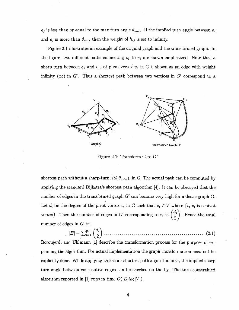
Definition 2.1 Given a graph G, a source node s, and a target node t, then a pair of

paths connecting s and t is called node disjoint if the paths do not share any node in

their interior.

Node Disjoint Paths Edge Disjoint Paths

Figure 2.2: Paths Types.

Figure 2.2 illustrates a pair of disjoint paths connecting s and t. The path-pair

shown in the left is node disjoint while the pair on the right side of the figure are just

edge-disjoint. The problem of computing shortest pair of s-t-disjoint paths was first

considered by Suurballe and Tarjan [13]. They reported an 0(mlog^i+m/n)n) algorithm

for solving the problem, where m and n are the number of edges and the number of

vertices respectively in the graph. Their technique is to convert the graph into a directed

graph that satisfies the anti-symmetric property. Note that a graph is said to satisfy

5

the anti-symmetric property if the presence of an edge (u, v) implies that an edge (u, u)

is not present. The algorithm uses complicated data structures which are difficult to

implement. Recently, a very simple algorithm to compute a pair of short length node-

disjoint paths connecting two vertices in a geometric network was reported in [8]. The

algorithm runs in <9(n2) time and is very simple to implement. This algorithm uses a

path-tagging technique for the construction of a path pair in a graph G. Since we will

be using this technique for developing an algorithm for turn constrained path pair we

briefly describe it below.

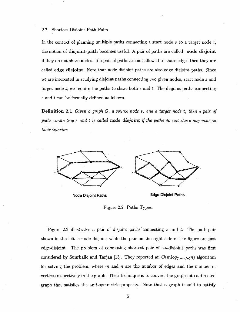
Figure 2.3: Shortest Path from s to t.

Consider a shortest path connecting s and t in a 2-d network as shown in Figure 2.3.

The shortest path is shown highlighted with thick edges. Now consider the set of edges

incident on the shortest path except those on s and t. We call these edges sleeve-edges.

The sleeve edges are drawn dashed in Figure 2.4. The process of directing sleeve edges

away from the path is called path-tagging. Let G1 denote the network obtained by path

tagging the shortest s-t-path p\ in a geometric graph G. If we compute a shortest s-t-path

P2 in G1 we find that px and pi are node disjoint; the computed path P2 is shown in Figure

2.5. However in some situations this technique of straight forward path tagging may fail

to work. This happens when the shortest s-t-path becomes a cut-path. A s-t-path P is

6

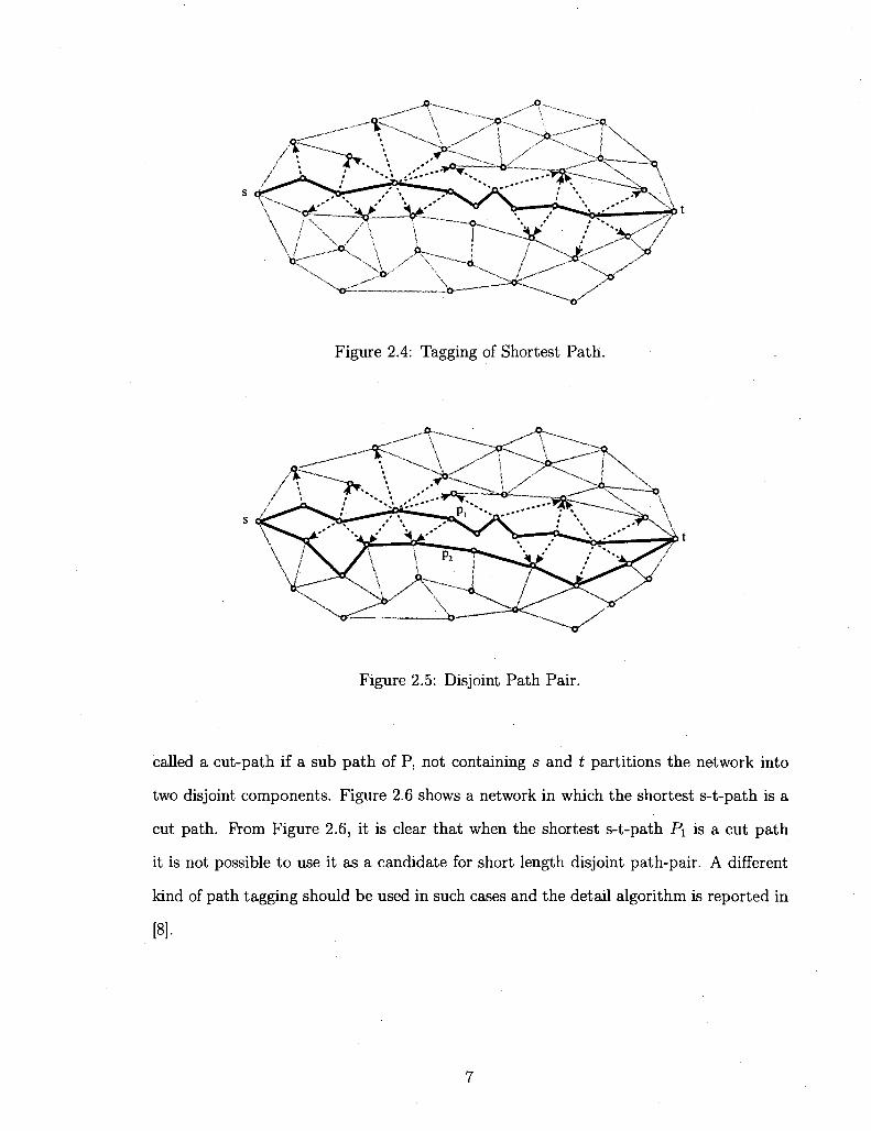
Figure 2.4: Tagging of Shortest Path.

Figure 2.5: Disjoint Path Pair.

called a cut-path if a sub path of P, not containing s and t partitions the network into

two disjoint components. Figure 2.6 shows a network in which the shortest s-t-path is a

cut path. From Figure 2.6, it is clear that when the shortest s-t-path Pi is a cut path

it is not possible to use it as a candidate for short length disjoint path-pair. A different

kind of path tagging should be used in such cases and the detail algorithm is reported in

[8].

7

Figure 2.6: Illustration of cut-path formation.

2.3 Constrained Disjoint Path Pairs

We are interested in the development of an efficient algorithm for constructing multiple

(k) node disjoint short length paths connecting two nodes in a geometric graph such

that the paths do not contain sharp turns. In particular, we start with the development

of an efficient algorithm for constructing a pair of (k = 2) node disjoint paths without

sharp turns. We combine the techniques for constructing the angle constrained shortest

path and node disjoint paths, briefly reviewed in the previous two sections, to solve the

problem which can be formally stated as follows.

Constrained Disjoint Path-Pair Problem (CDPP)

Given: A planar geometric graph G(V, E), start node s, target node t and maximum

turn angle 0max.

Question: Construct a short-length node disjoint path-pair p\ and P2 connecting s to

t such that the paths are of short lengths and do not contain a turn angle greater than

Vmax •

To make sure that the path-pair do not have a turn angle greater than 6max we use the

graph transformation method formulated by Boroujerdi and Uhlmann [1]. Furthermore,

to make sure that the pair are disjoint in their interior and are of short length, we use the

path-tagging technique presented in [8]. The approach is first to find the turn constrained

shortest path P connecting s to t. We then check whether P is a cut-path or not for

8

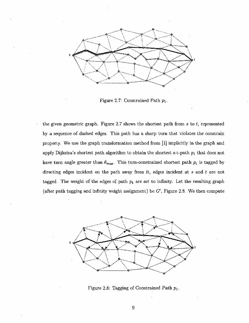
Figure 2.7: Constrained Path p\-.

the given geometric graph. Figure 2.7 shows the shortest path from s to t, represented

by a sequence of dashed edges. This path has a sharp turn that violates the constrain

property. We use the graph transformation method from [1] implicitly in the graph and

apply Dijkstra's shortest path algorithm to obtain the shortest s-t-path pi that does not

have turn angle greater than 9max. This turn-constrained shortest path p\ is tagged by

directing edges incident on the path away from it, edges incident at s and t are not

tagged. The weight of the edges of path px are set to infinity. Let the resulting graph

(after path tagging and infinity weight assignment) be G', Figure 2.8. We then compute

Figure 2.8: Tagging of Constrained Path-pi.

9

the turn constrained shortest path p2 between s and t in G'. The path p2 is edge disjoint

due to the path tagging. The pair of paths p\ and p2 give the short length disjoint path

pair between s and t. (If p\ is a cut path then the boundary of the graph is tagged by

following the approach given in [8]). Figure 2.9 shows the final short length disjoint path

pair. A sketch of the Turn Constrained Disjoint Path Pair algorithm is shown below.

Figure 2.9: Constrained Disjoint Path Pair pi and p2.

10

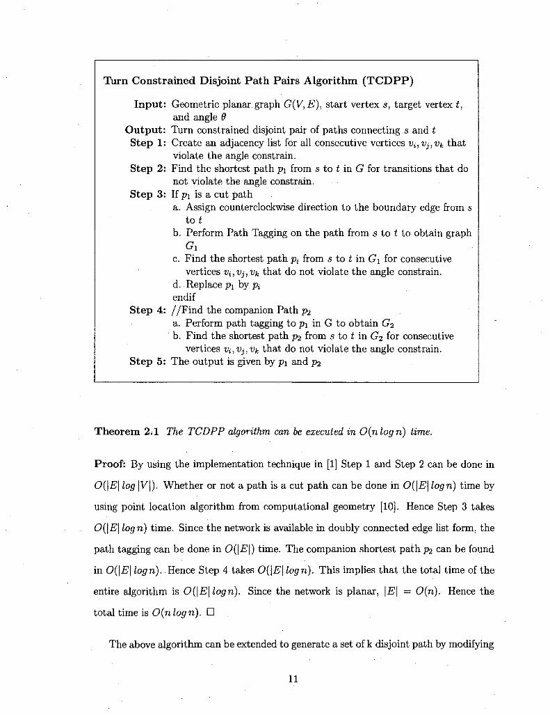
Turn Constrained Disjoint Path Pairs Algorithm (TCDPP)

Input: Geometric planar graph G(V, E), start vertex s, target vertex t, and angle 9

Output: Turn constrained disjoint pair of paths connecting s and t Step 1: Create an adjacency list for all consecutive vertices Vi,Vj,Vk that

violate the angle constrain. Step 2: Find the shortest path pi from s to t in G for transitions that do

not violate the angle constrain. Step 3: If pi is a cut path

a. Assign counterclockwise direction to the boundary edge from s to t

b. Perform Path Tagging on the path from s to t to obtain graph d

c. Find the shortest path p^ from s to t in G\ for consecutive vertices Vi,Vj,Vk that do not violate the angle constrain.

d. Replace p\ by pi endif

Step 4: //Find the companion Path pi a. Perform path tagging to p\ in G to obtain G2 b. Find the shortest path p2 from s to t in G2 for consecutive

vertices Vi, Vj, Vk that do not violate the angle constrain. Step 5: The output is given by p\ and pi

Theorem 2.1 The TCDPP algorithm can be executed in 0(nlogn) time.

Proof: By using the implementation technique in [1] Step 1 and Step 2 can be done in

0(\E\ log \V\). Whether or not a path is a cut path can be done in 0(\E\ logn) time by

using point location algorithm from computational geometry [10]. Hence Step 3 takes

0(\E\ logn) time. Since the network is available in doubly connected edge list form, the

path tagging can be done in Od^l) time. The companion shortest path p^ can be found

in 0(\E\ logn). Hence Step 4 takes 0(\E\ logn). This implies that the total time of the

entire algorithm is 0(\E\logn). Since the network is planar, \E\ = 0(n). Hence the

total time is 0(nlogn). •

The above algorithm can be extended to generate a set of k disjoint path by modifying

11

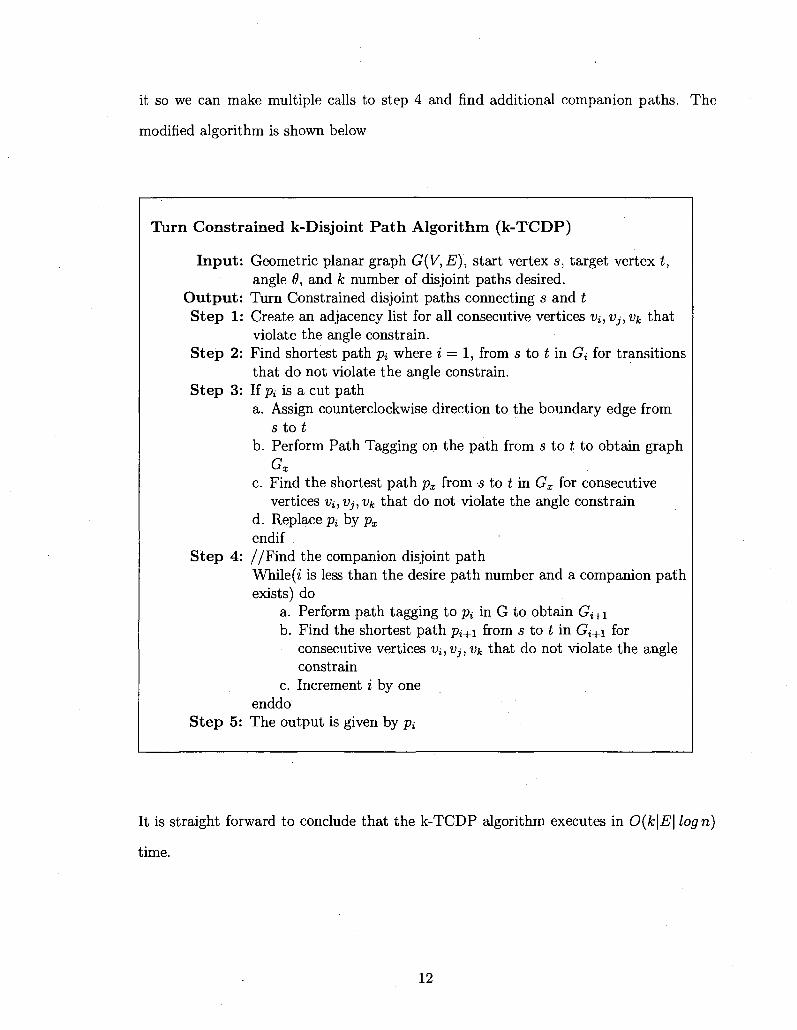
it so we can make multiple calls to step 4 and find additional companion paths. The

modified algorithm is shown below

Turn Constrained k-Disjoint Path Algorithm (k-TCDP)

Input: Geometric planar graph G(V, E), start vertex s, target vertex t, angle 0, and k number of disjoint paths desired.

Output: Turn Constrained disjoint paths connecting s and t Step 1: Create an adjacency list for all consecutive vertices Vi,Vj,Vk that

violate the angle constrain. Step 2: Find shortest path Pi where i = 1, from s to t in Gj for transitions

that do not violate the angle constrain. Step 3: If pi is a cut path

a. Assign counterclockwise direction to the boundary edge from s to t

b. Perform Path Tagging on the path from s to t to obtain graph Gx

c. Find the shortest path px from s to t in Gx for consecutive vertices Vi,Vj,Vk that do not violate the angle constrain

d. Replace Pi by px

endif Step 4: //Find the companion disjoint path

While (i is less than the desire path number and a companion path exists) do

a. Perform path tagging to Pi in G to obtain Gi+\ b. Find the shortest path pi+\ from s to t in Gi+\ for

consecutive vertices Vi, Vj, Vk that do not violate the angle constrain

c. Increment i by one enddo

Step 5: The output is given by pt

It is straight forward to conclude that the k-TCDP algorithm executes in 0(A:|£7| logn)

time.

12

CHAPTER 3

CONSTRAINT SHORTEST PATH MAP (CSPM)

3.1 Shortest Path Map (SPM)

Consider a collection of convex obstacles Qi, Q2,.... Qk in two dimensions. For computing

collision-free shortest path from start points s to any other goal points gi,g2, •••,9m , the

notion of the shortest path map (SPM) has been used very successfully [7, 11]. Broadly

speaking, the shortest path map induced by a collection of obstacles and a source point

s is the partitioning of the free space (space without obstacles) into regions such that

the shortest path from s to any point in a region passes through the same set of obstacle

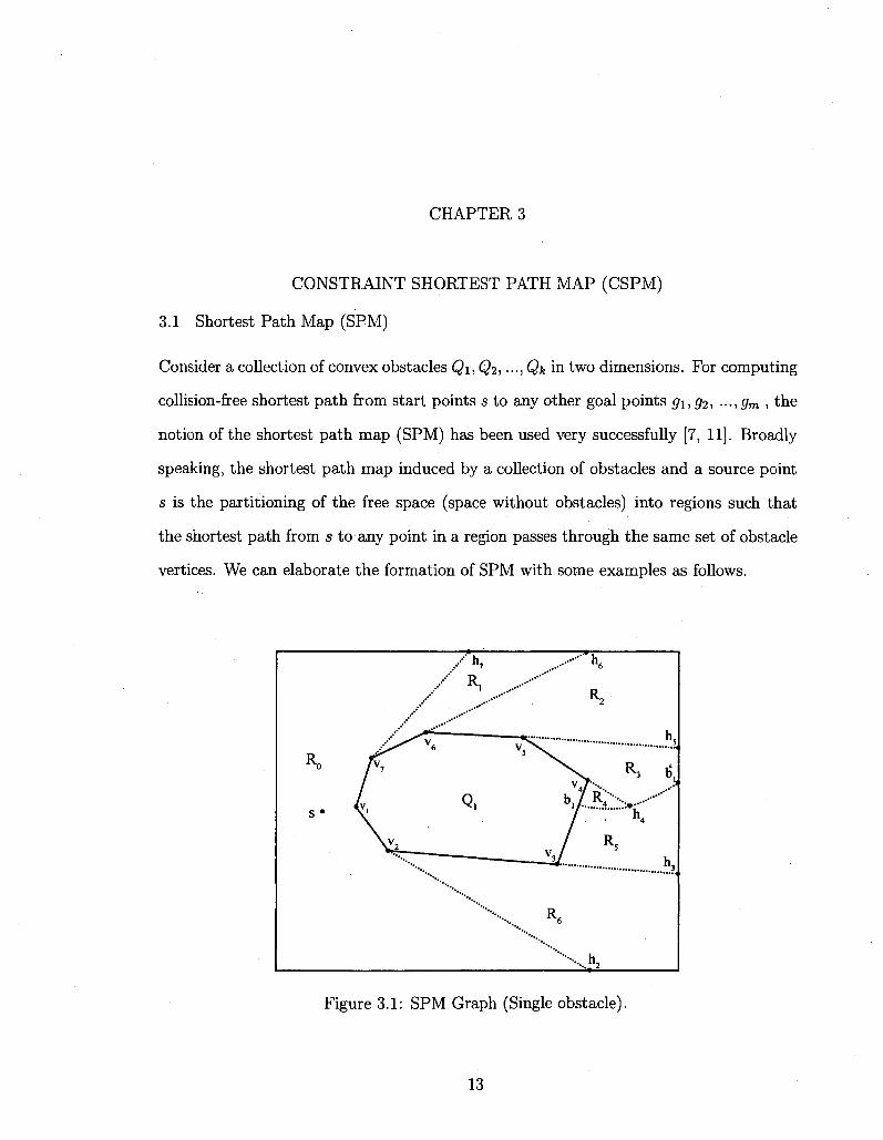
vertices. We can elaborate the formation of SPM with some examples as follows.

s • X

V6

.A ' R,

Q.

V 5 S

••••-'K

^

/

* 6

"""'-•••-h

K 5

Figure 3.1: SPM Graph (Single obstacle).

13

First consider only one obstacle Qi and a source point s enclosed in a rectangular box

as shown in Figure 3.1 (drawn by solid line segments). Let the list of vertices of obstacle

Qx be vi, t>2, •••,Vm when the boundary is traversed in the counterclockwise direction.

Consider two supporting rays emanating from s and supporting Q\ at vertices Vi and

Vj. Such vertices are called support-vertices. Let /i, and hj be the points of intersection

(hit-points) of the supporting rays with the enclosing rectangular box. The line segment

(vi,'hi) on the supporting rays is referred to as a connecting-segment, shown in Figure

3.1 as dashed segments.

d(v,)

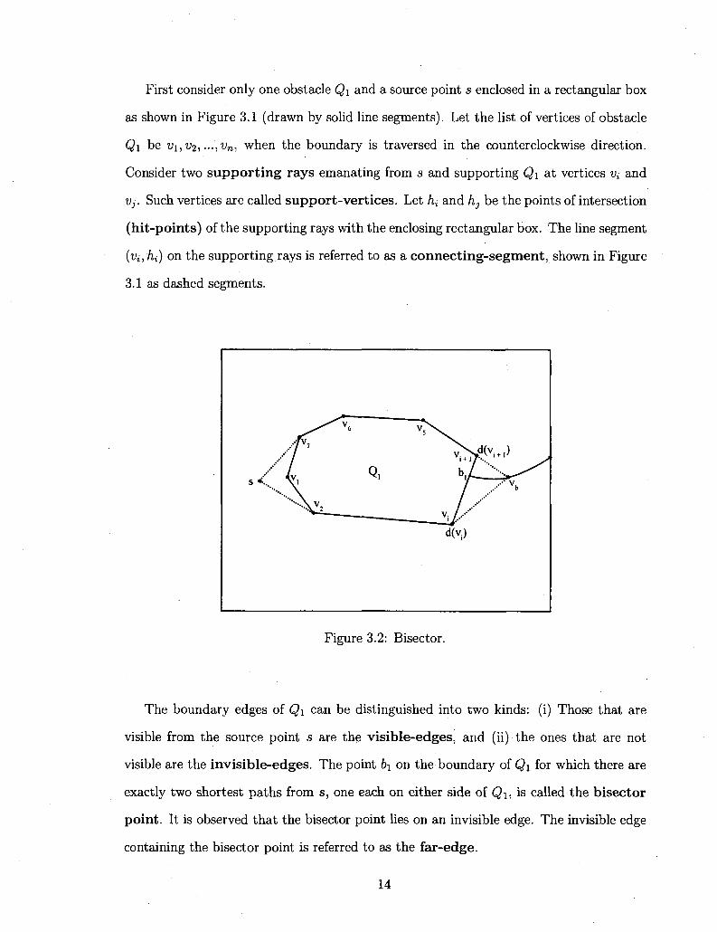
Figure 3.2: Bisector.

The boundary edges of Q\ can be distinguished into two kinds: (i) Those that are

visible from the source point s are the visible-edges, and (ii) the ones that are not

visible are the invisible-edges. The point b\ on the boundary of Q\ for which there are

exactly two shortest paths from s, one each on either side of Qi, is called the bisector

point. It is observed that the bisector point lies on an invisible edge. The invisible edge

containing the bisector point is referred to as the far-edge.

14

The locus of the points which are equidistant from s form a branch of a hyperbola

[7] as shown in Figure 3.2. Let Vi and Vi+i be the vertices that define the far edge, then

d(vi) will be the shortest counterclockwise distance from s to vt and d(vi+i) will be the

shortest clockwise distance from s to 1 +1. If Vb is a point on the hyperbola branch,

then let length(vi,Vb) be the length of the segment (i>j, t>&) and length(vi+i,Vb) be the

length of the segment (vi+i,Vb), thus d(vi) + length(vi,vb) = d(vi+i) + length(vi+i,Vb)

and length(vi+i, Vb) — length(vi,Vb) = d(v{) — d(vi+i) where vt and Vi+i are the foci of the

hyperbola and Vb belongs to one of the two branches of the hyperbola. If d(vi) > d(ui+1),

then Vb belongs to the branch closest to vi} otherwise it belongs to the branch closest to

If we traverse the boundary of Q\ in a counterclockwise direction, starting from the

vertex closest to s, the invisible edges encountered before reaching the far-edge are termed

as group-1 invisible edges. The other invisible-edges that are encountered after the

far-edge are termed as group-2 invisible edges.

Connecting-segments can be defined for invisible edges other than the far edge. For an

invisible edge (vi,Vi+i) in group-1, the corresponding connecting-segment (vi+i,hi+i) is >

formed by considering the ray (vi, vi+i). On the other hand, for an invisible edge (i>i+i, Uj) >

in group-2, the connecting-segment (vi,hi) is formed by considering ray (ui+1)Ui). It is

noted that the hit point hi for constructing the connecting segments for the invisible

edges could be either on the enclosing rectangle or on the bisector parabola.

The set of connecting segments and hyperbola branches partition the free space into

q regions RQ, i?i, i?2, ••-, Rq, where q is the total number of connecting segments. Corre­

sponding to each connecting segment (w,, hi) there is a unique free-region. A connecting

segment will partition a region in at most two new smaller regions if and only if both Vi

and hi are on the boundary of the original region, otherwise the connecting segment will

join the obstacle boundary with the region boundary.

Definition 3.1 The collection of free-regions formed by the set of connecting segments

and bisector hyperbola branches is called the Shortest-Path Map (SPM) for source point

15

s. Figure 3.1 shows the shortest path map for one convex obstacle, where there are seven

free regions.

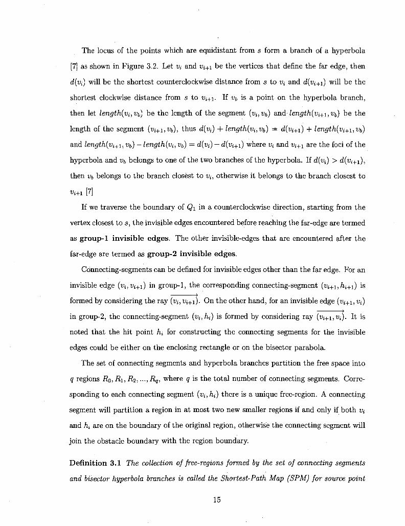
Figure 3.3: SPM Graph (two obstacles).

For more than one obstacle, the corresponding shortest path map can be defined

similarly. Support vertices are again defined by considering support rays. The support

rays can hit either the boundary of the enclosing rectangle, the boundary of another

obstacle or the bisector hyperbola branch. We also need to construct possible connecting

edges by considering the connecting-segments incident to a vertex V{ as secondary source

vertices. The shortest path map for two obstacles is shown in Figure 3.3, where there are

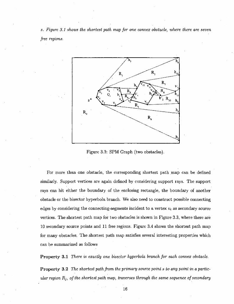
10 secondary source points and 11 free regions. Figure 3.4 shows the shortest path map

for many obstacles. The shortest path map satisfies several interesting properties which

can be summarized as follows

Property 3.1 There is exactly one bisector hyperbola branch for each convex obstacle.

Property 3.2 The shortest path from the primary source point s to any point in a partic­

ular region Rj, of the shortest path map, traverses through the same sequence of secondary

16

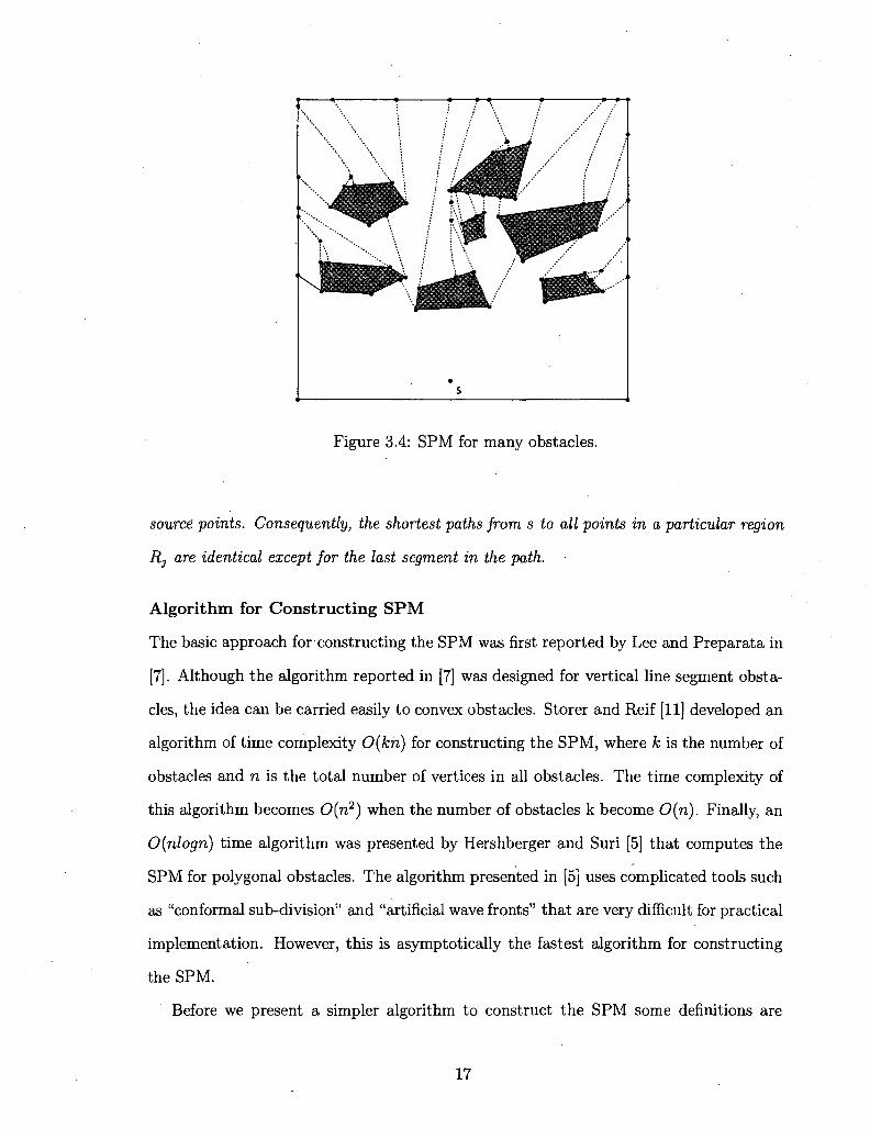
Figure 3.4: SPM for many obstacles.

source points. Consequently, the shortest paths from s to all points in a particular region

Rj are identical except for the last segment in the path.

Algorithm for Constructing S P M

The basic approach for constructing the SPM was first reported by Lee and Preparata in

[7]. Although the algorithm reported in [7] was designed for vertical line segment obsta­

cles, the idea can be carried easily to convex obstacles. Storer and Reif [11] developed an

algorithm of time complexity 0(kn) for constructing the SPM, where k is the number of

obstacles and n is the total number of vertices in all obstacles. The time complexity of

this algorithm becomes 0(n2) when the number of obstacles k become 0(n). Finally, an

Oinlogn) time algorithm was presented by Hershberger and Suri [5] that computes the

SPM for polygonal obstacles. The algorithm presented in [5] uses complicated tools such

as "conformal sub-division" and "artificial wave fronts" that are very difficult for practical

implementation. However, this is asymptotically the fastest algorithm for constructing

the SPM.

Before we present a simpler algorithm to construct the SPM some definitions are

17

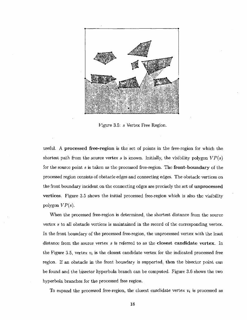
Figure 3.5: s Vertex Free Region.

useful. A processed free-region is the set of points in the free-region for which the

shortest path from the source vertex s is known. Initially, the visibility polygon VP(s)

for the source point s is taken as the processed free-region. The front-boundary of the

processed region consists of obstacle edges and connecting edges. The obstacle vertices on

the front boundary incident on the connecting edges are precisely the set of unprocessed

vertices. Figure 3.5 shows the initial processed free-region which is also the visibility

polygon VP(s).

When the processed free-region is determined, the shortest distance from the source

vertex s to all obstacle vertices is maintained in the record of the corresponding vertex.

In the front boundary of the processed free-region, the unprocessed vertex with the least

distance from the source vertex s is referred to as the closest candidate vertex. In

the Figure 3.5, vertex Vi is the closest candidate vertex for the indicated processed free

region. If an obstacle in the front boundary is supported, then the bisector point can

be found and the bisector hyperbola branch can be computed. Figure 3.6 shows the two

hyperbola branches for the processed free region.

To expand the processed free-region, the closest candidate vertex Vi is processed as

18

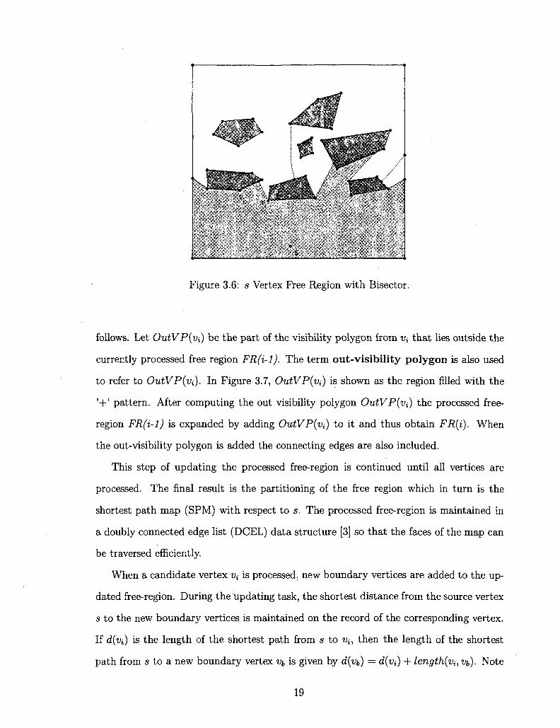
Figure 3.6: s Vertex Free Region with Bisector.

follows. Let OutVP(vi) be the part of the visibility polygon from Vi that lies outside the

currently processed free region FR(i-l). The term out-visibility polygon is also used

to refer to OutVP{vi). In Figure 3.7, OutVPivi) is shown as the region filled with the

'+' pattern. After computing the out visibility polygon OutVPivi) the processed free-

region FR(i-l) is expanded by adding OutVP(vi) to it and thus obtain FR(i). When

the out-visibility polygon is added the connecting edges are also included.

This step of updating the processed free-region is continued until all vertices are

processed. The final result is the partitioning of the free region which in turn is the

shortest path map (SPM) with respect to s. The processed free-region is maintained in

a doubly connected edge list (DCEL) data structure [3] so that the faces of the map can

be traversed efficiently.

When a candidate vertex v^ is processed, new boundary vertices are added to the up­

dated free-region. During the updating task, the shortest distance from the source vertex

s to the new boundary vertices is maintained on the record of the corresponding vertex.

If d(vi) is the length of the shortest path from s to V{, then the length of the shortest

path from s to a new boundary vertex Vb is given by d(vb) = d(yi) + length^, vt,). Note

19

Figure 3.7: Vi Generated Free Region.

that the line segment connecting vt to Vb lies completely in the free-region. Furthermore,

in the structure of Vb, a reference to the previous vertex in the shortest path from the

source vertex s is recorded. This makes it easy to construct the actual shortest paths.

Definition 3.2 A vertex v on the boundary of SPM(k) is called Typel if both boundary

edges incident in v are the edges of the obstacle. In Figure 3.5, Vj is a Typel vertex.

Definition 3.3 A vertex v on the boundary ofSPM(k) is called Type2 if it is an obstacle

vertex and a connecting edge is formed by extending an obstacle edge incident at V{. In

Figure 3.5 v^ is a Type2 vertex.

Definition 3.4 An obstacle Q on the boundary of SPM(k) is called boundary sup­

ported if Q is tangentially supported by two connecting edges.

A formal description of the Algorithm is as follows.

20

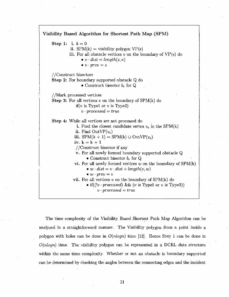
Visibility Based Algorithm for Shortest Path Map (SPM)

Step 1: i. k = 0 ii. SPM(k) = visibility polygon VP(s) iii. For all obstacle vertices v on the boundary of VP(s) do

• v • dist = length(s, v) • v • prev = s

/ /Construct bisectors Step 2: For boundary supported obstacle Q do

• Construct bisector br for Q

/ /Mark processed vertices Step 3: For all vertices v on the boundary of SPM(k) do

if(u is Typel or v is Type2) v • processed — true

Step 4: While all vertices are not processed do i. Find the closest candidate vertex vc in the SPM(k) ii. Find OutVP(wc)

iii. SPM(k + 1) = SPM(k) U OutVP(vc) iv. k = k + 1 / /Construct bisector if any v. For all newly formed boundary supported obstacle Q

• Construct bisector br for Q vi. For all newly formed vertices w on the boundary of SPM(k)

• w • dist — v • dist + length(v, w) • w • prev = v

vii. For all vertices v on the boundary of SPM(k) do • if((!t> • processed) &&; (v is Typel or v is Type2))

v • processed = true

The time complexity of the Visibility Based Shortest Path Map Algorithm can be

analyzed in a straightforward manner. The Visibility polygon from a point inside a

polygon with holes can be done in 0(nlogn) time [12]. Hence Step 1 can be done in

0(nlogn) time. The visibility polygon can be represented in a DCEL data structure

within the same time complexity. Whether or not an obstacle is boundary supported

can be determined by checking the angles between the connecting edges and the incident

21

obstacle edge. Once an obstacle is identified as 'boundary-supported', the corresponding

bisector can be determined in time proportional to the number of vertices in the obstacle.

Hence Step 2 takes 0{n) time. Whether or not a vertex v on the boundary of SPM(K)

is Typel (or Type2) can be done in constant time by checking the edges incident on

it. Hence Step 3 take 0(n) time. The closest candidate vertex vc can be determined

by simply checking the distance to each vertex on the boundary of SPM(k) which takes

0{n) time. OutVP(vc) can be computed in 0{nlogn) time by using a variation of the

standard visibility polygon algorithm. The union of SPMK and OutVP(vc) can be done

in 0(n) time. Hence Step 4 iii and Step 4 iv can be done in 0{n) time. Similarly each

of Step 4 v, Step 4 vi, and Step 4 vii can be done in 0(n) time. The while loop in Step

4 can execute in 0(n) time. Hence total time for Step 4 is 0(n2logn). This implies that

the total time for the entire algorithm is 0(n2logn).

3.2 Constrained Shortest Path Map (CSPM)

The standard shortest path map (SPM) can be used for computing repeated shortest path

queries from a fixed source vertex s to several target vertices. If we want to compute the

shortest path between the source vertex s and a target vertex t such that the path does

not contain sharp turns, then SPM can not be used. We want to construct a constrained

shortest path map (CSPM) for a collection of convex polygonal obstacles such that it can

be used to compute the shortest path that does not contain sharp turns. The problem

can be formally stated as follows

22

Constrained Shortest Path Map Problem

Given: (i) A collection of convex polygonal obstacles

(ii) Source Vertex s

(iii) Turn angle 6

Question: Construct a constrained shortest path map (CSPM) such that it

can be used to find the shortest path between s and any,target point t such

that the path has turns no more than 9. The Path can take a turn only at the

vertices.

Figure 3.8: Illustrating Restricted Faces and Forbidden regions.

Our approach for constructing the CSPM is to characterize forbidden regions in

the standard SPM that can not be reached by any path that can turn only on vertices

and for which the turn angle is no more than 6. Consider a face ft rooted at a secondary

source vertex i>j. In Figure 3.8, the region bounded by Vi, hit hk, ffc, h is the face /j rooted

at Vi. If the internal angle of /j at i>, is greater than 0 then not all points inside face

fi are reachable by a path that turns at V{. Such a face which can not be completely

reached by the shortest path from the source vertex s is referred to as a restricted face.

23

A restricted face / ; can be partitioned into two parts by a limit chord of the face. The

limiting chord ViCi is such that the angle hiViCi is exactly equal to 9. The portion of fa

not reachable by the shortest path with a turn at Vi greater than 9, is called a forbidden

region, which is shown by a hashed pattern in Figure 3.8. The remaining portion of fa

is the reacheable region. The figure also shows the forbidden region corresponding to

the restricted face rooted at vertex Vj. To construct a constrained shortest path map

(CSPM) we start from the standard shortest path map (SPM). Each face of the SPM is

examined to determine whether or not it is a restricted face. If a face fa is restricted then

it is partitioned into two parts to identify the corresponding forbidden component. Since

the standard SPM is available in a doubly connected edge list form, restricted faces can

be easily identified. A restricted face can be processed to extract the forbidden region by

constructing the limit chord. The limit chord can be constructed in time proportional to

the number of vertices in the restricted face. A formal sketch of the algorithm is listed

as the Constrained Shortest Path Map Algorithm.

Property 3.3 For points that lie within a forbidden region, no path exist in the CSPM

back to s.

Theorem 3.1 The constrained shortest path map can be constructed in 0(fa(n)) time,

where n is the total number of vertices in the obstacles and fs(n) is the time for computing

the standard SPM.

24

Constrained Shortest Path Map (CSPM) Algorithm

Input: A collection of obstacles, start point s, maximum turn angle 9

Output: Constrained Shortest Path Map.

Step 1: Construct the standard shortest path map (SPM) with source vertex s and represent it DCEL form.

Step 2: Identify and mark all secondary source vertices in the SPM

Step 3: For each face in /, corresponding to secondary source vertex Vi do If (fi is a restricted face)

partition fi by constructing the limiting chi

Step 4: Output resulting map as CSPM

Proof: Step 1 takes 0(fs(n)) time. Once the SPM is available in DCEL data structure,

the secondary source vertex of a face can be determined by examining the value of the

shortest path distance from s, (in each face, the vertex with the least distance from s is

the secondary source vertex). Hence Step 2 takes 0{n) time. Whether or not a face fi is

restricted can be determined by comparing the interior angle of the source vertex with

the maximum allowed angle 9 and this takes constant time. The limiting chord and its

use in partitioning the face can be done in time proportional to the number of vertices

in the face. Hence Step 3 takes 0(n) time. The total time for the whole algorithm is

0(fs(n)). D

3.3 Extending CSPM to add partially forbidden region

Definition 3.5 In a CSPM, a region partially bounded by bounding rectangle edges, ob­

stacle edges, limit chords and at least one connecting segment is called a partially for­

bidden region.

Definition 3.6 A region in the CSPM containing a point for which there exist a path

back to s in which all turn angles are less than 9 and it is not the shortest path is called

25

a reacheable region

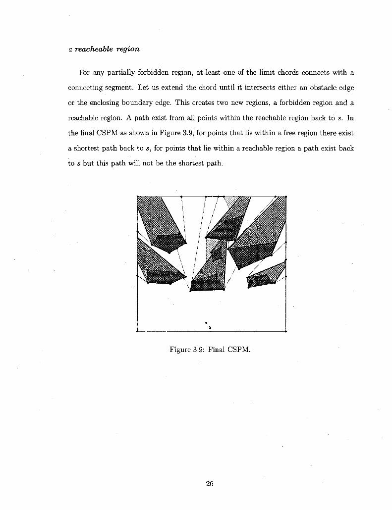
For any partially forbidden region, at least one of the limit chords connects with a

connecting segment. Let us extend the chord until it intersects either an obstacle edge

or the enclosing boundary edge. This creates two new regions, a forbidden region and a

reachable region. A path exist from all points within the reachable region back to s. In

the final CSPM as shown in Figure 3.9, for points that lie within a free region there exist

a shortest path back to s, for points that lie within a reachable region a path exist back

to s but this path will not be the shortest path.

Figure 3.9: Final CSPM.

26

CHAPTER 4

IMPLEMENTATION

This chapter describes an implementation of the two prototype programs used to study

the Turn Constrained Disjoint Path and the Constrained Shortest Path Map problems.

The programs were implemented in Java, using version 1.4.2

4.1 Constrained Disjoint Path Interface

The implementation of this prototype permits the user to create a network consisting

of obstacles which can be edited by adjusting the edges and vertices. Additionally, the

source and target points can be changed. Once the network is created the user can

initiate the execution of the program to generate the visibility edges and to calculate the

shortest disjoint paths from the source vertex s to a target vertex t.

4.1.1 Interface Description

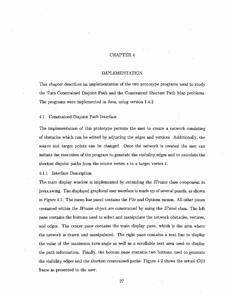
The main display window is implemented by extending the JFrame class component in

javax.swing. The displayed graphical user interface is made up of several panels, as shown

in Figure 4.1. The menu bar panel contains the File and Options menus. All other panes

contained within the JFrame object are constructed by using the JPanel class. The left

pane contains the buttons used to select and manipulate the network obstacles, vertices,

and edges. The center pane contains the main display pane, which is the area where

the network is drawn and manipulated. The right pane contains a text line to display

the value of the maximum turn-angle as well as a scrollable text area used to display

the path information. Finally, the bottom pane contains two buttons used to generate

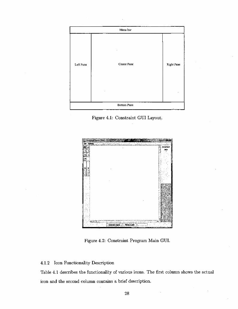
the visibility edges and the shortest constrained paths. Figure 4.2 shows the actual GUI

frame as presented to the user.

27

Menu bar

Left Pane Center Pane Right Pane

Bottom Pane

Figure 4.1: Constraint GUI Layout.

-- - j w ]

Figure 4.2: Constraint Program Main GUI.

4.1.2 Icon Functionality Description

Table 4.1 describes the functionality of various icons. The first column shows the actual

icon and the second column contains a brief description.

28

Table 4.1: Icon description. Icon

*

* »

t.B

-B ' ft^WB

- •

*-*

S T

Description

Enables the select mode

If the select mode is enabled, and an obstacle has been selected, the user can change the position of the obstacle by dragging it with the mouse

Allows the user to add a new obstacle to the graph

Used for removing the selected obstacle Used for splitting an edge of the selected obstacle. The splitting is done by introducing a new vertex

Used for removing a vertex of the selected obstacle. The vertex closest to the mouse cursor is selected Used for updating the coordinates of the closest vertex (from the mouse cursor) of the selected obstacle For Moving the source vertex to a selected mouse cursor position For moving the target vertex to a selected mouse cursor position

4.1.3 Program menu items

The program has two menu items: File and Options. The File menu items enable the user

to (i) clear the display screen, (ii) start a new network, (iii) retrieve and open previously

saved files, and (iv) save a generated network to a file. A brief description of the File

items is provided in Table 4.2. A similar description is provided for the Options items

as described in Table 4.3. Figure 4.3 shows the GUI representation of the Options menu

items.

Table 4.2: File menu Items description. File Item Description

New Clears the center display panel. Ready for a new network Open File Brings up a file selection panel, user can choose an existing

graph file Save File Brings up a file save panel. The user can save a new file or

replace an existing file

29

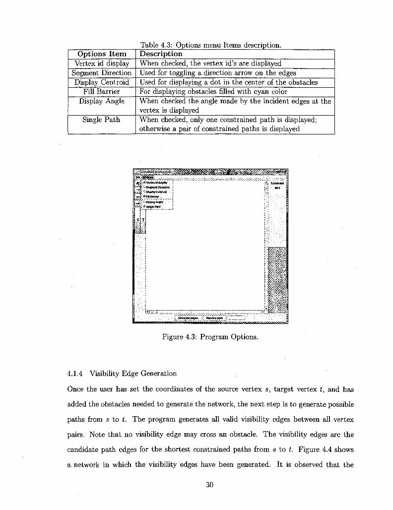
Table 4.3: Options menu Items description. Options Item

Vertex id display Segment Direction Display Centroid

Fill Barrier Display Angle

Single Path

Description When checked, the vertex id's are displayed Used for toggling a direction arrow on the edges Used for displaying a dot in the center of the obstacles For displaying obstacles filled with cyan color When checked the angle made by the incident edges at the vertex is displayed When checked, only one constrained path is displayed; otherwise a pair of constrained paths is displayed

„ <mAm^:ifcai$^wgm'i

f ^ i ^Vartmtia&spfcgr CcBSoaas

l ' . i<mr •s.$nMW*0$m; •• i'<_ ttiprafi^KWtr

Figure 4.3: Program Options.

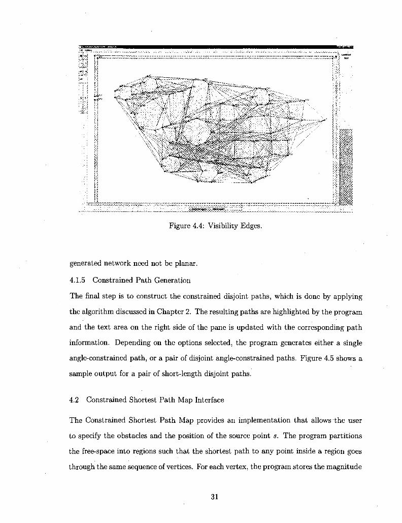
4.1.4 Visibility Edge Generation

Once the user has set the coordinates of the source vertex s, target vertex t, and has

added the obstacles needed to generate the network, the next step is to generate possible

paths from s to t. The program generates all valid visibility edges between all vertex

pairs. Note that no visibility edge may cross an obstacle. The visibility edges are the

candidate path edges for the shortest constrained paths from s to t. Figure 4.4 shows

a network in which the visibility edges have been generated. It is observed that the

30

4MWMMM0M J$|M>*»*»

Figure 4.4: Visibility Edges.

generated network need not be planar.

4.1.5 Constrained Path Generation

The final step is to construct the constrained disjoint paths, which is done by applying

the algorithm discussed in Chapter 2. The resulting paths are highlighted by the program

and the text area on the right side of the pane is updated with the corresponding path

information. Depending on the options selected, the program generates either a single

angle-constrained path, or a pair of disjoint angle-constrained paths. Figure 4.5 shows a

sample output for a pair of short-length disjoint paths.

4.2 Constrained Shortest Path Map Interface

The Constrained Shortest Path Map provides an implementation that allows the user

to specify the obstacles and the position of the source point s. The program partitions

the free-space into regions such that the shortest path to any point inside a region goes

through the same sequence of vertices. For each vertex, the program stores the magnitude

31

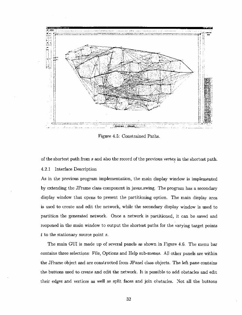
ij» a » * w • • • • . . - ' • ' , . , - • ' • . •

Figure 4.5: Constrained Paths.

of the shortest path from s and also the record of the previous vertex in the shortest path.

4.2.1 Interface Description

As in the previous program implementation, the main display window is implemented

by extending the JFrame class component in javax.swing. The program has a secondary

display window that opens to present the partitioning option. The main display area

is used to create and edit the network, while the secondary display window is used to

partition the generated network. Once a network is partitioned, it can be saved and

reopened in the main window to output the shortest paths for the varying target points

t to the stationary source point s.

The main GUI is made up of several panels as shown in Figure 4.6. The menu bar

contains three selections: File, Options and Help sub-menus. All other panels are within

the JFrame object and are constructed from JPanel class objects. The left pane contains

the buttons used to create and edit the network. It is possible to add obstacles and edit

their edges and vertices as well as split faces and join obstacles. Not all the buttons

32

Menu bar

Left Pane Center Pane Right Pane

Bottom Pane

Figure 4.6: Planar GUI Layout.

Menu bar

Display Pane Right Pane

Bottom Pane

Figure 4.7: Partition GUI Layout.

are functional, buttons that are functional will change color to cyan when selected. The

center pane contains the main display pane. This is the area in which the network will be

drawn and manipulated. The right pane contains two text boxes: one is used to display

the cursor's x-y coordinate as it moves over the center pane and the second one is a large

33

scrollable text area which is updated with the network information. Finally, the bottom

pane contains two buttons: the partition button which will open the secondary window

to present the partition GUI, and the Shortest Distance button which will trigger the

program to calculate a path from the source vertex to the target vertex for the network

that has been previously partitioned.

The secondary display window also contains several panels as shown in Figure 4.7.

The menu bar contains the File and Options menus. The center pane is again the main

display pane, and the right pane contains a scrollable text area that displays the network

information. Finally, the bottom pane contains a single button that initiates the network

partition action. Figure 4.8 and Figure 4.9 show the actual GUIs presented to the user

by the program.

1£2£* _ „< . ' n J i l M & l v. JHSSK J^Sisim

m \t&M$l

lOKMft •

Figure 4.8: Planar Program Main GUI.

4.2.2 Icon Functionality Description

Table 4.4 and Table 4.5 show the description of the icons functionality. The first col­

umn shows the image of the icon and the second column gives a brief description of its

functionality.

34

%*)&&* Vsy* ^ i ^-."^^^^jS^^^g-,*", y&iiiis

j f iWa^Wa^

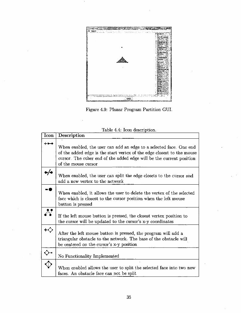
Figure 4.9: Planar Program Partition GUI.

Table 4.4: Icon description. Icon

+•-»

* / *

- •

A*

+<>

< > *

4>

Description

When enabled, the user can add an edge to a selected face. One end of the added edge is the start vertex of the edge closest to the mouse cursor. The other end of the added edge will be the current position of the mouse cursor

When enabled, the user can split the edge closets to the cursor and add a new vertex to the network

When enabled, it allows the user to delete the vertex of the selected face which is closest to the cursor position when the left mouse button is pressed

If the left mouse button is pressed, the closest vertex position to the cursor will be updated to the cursor's x-y coordinates

After the left mouse button is pressed, the program will add a triangular obstacle to the network. The base of the obstacle will be centered on the cursor's x-y position

No Functionality Implemented

When enabled allows the user to split the selected face into two new faces. An obstacle face can not be split

35

Table 4.5: Icon description continued. Icon

C

K

s T

+ + f f

Description Create a connection between two vertices

When enable the user can select a face on the graph. Used as preliminary step before splitting face and edges Updates the x-y coordinates of the source vertex to the current cursor location Updates the x-y coordinates of the target vertex to the current cursor location

No Functionality Implemented

No Functionality Implemented

No Functionality Implemented

No Functionality Implemented

Table 4.6: File menu Items description. File Item Open File

Save File

New Export to Xfig

Description Brings up a file selection panel, user can choose an existing graph file Brings up a file save panel, the user can save a new file or replace an existing file Clears the center display panel, ready for a new graph Brings up file save panel, the file is saved in Xfig file format

Table 4.7: Options and Help menu Items description. Options I tem

HalfEdge Display Help Item

Help Contents

Description When checked displays the half edges individually Description Access 'to help information

4.2.3 Program Submenu Description

The program's main GUI has three menu selections: File, Options, and Help. The File

menu items enables the user to retrieve and open a previously saved file or to save the

currently displayed network to a file, or to clear the display-screen. It also has an option

36

to export the network into Xfig format. A brief description of the File items is given in

Table 4.6. The Options and Help items are described in Table 4.7. Figure 4.10 shows

the GUI representation of the Options sub-menu items.

*

w

>

• -- Pwwm •.'. i:.m>mmot^ane*!::

&• ^gsaBawaaamsaawsg^w^^^ w t w ^

Figure 4.10: Planar Program File Options.

The secondary program GUI also has File and Options menus. The File menu has

a single function that allows the user to save a network that has been partitioned. The

Options menu lets the user enable/disable a step function. A detailed description of the

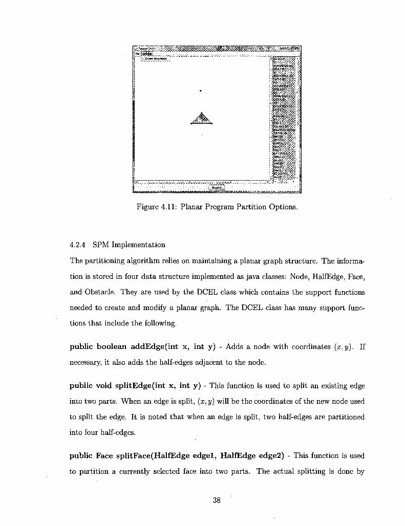
sub menus is shown on Table 4.8. Figure 4.11 shows the GUI with the Options menu as

presented to the user.

Tal File I tem

« Save File

Options I tem Enable Step Mode

)le 4.8: File and Options menu Items description. Description Brings up a file save panel, the user can save the partitioned file Description Displays each step as program processes the vertices

37

mf^Sm^ii^^M.', **"•****

$

KS

?£$$£&

Pi t t i te

MASS

users-

Figure 4.11: Planar Program Partition Options.

4.2.4 SPM Implementation

The partitioning algorithm relies on maintaining a planar graph structure. The informa­

tion is stored in four data structure implemented as Java classes: Node, HalfEdge, Face,

and Obstacle. They are used by the DCEL class which contains the support functions

needed to create and modify a planar graph. The DCEL class has many support func­

tions that include the following.

public boolean addEdge(int x, int y) - Adds a node with coordinates (x,y). If

necessary, it also adds the half-edges adjacent to the node.

public void splitEdge(int x, int y) - This function is used to split an existing edge

into two parts. When an edge is split, (x, y) will be the coordinates of the new node used

to split the edge. It is noted that when an edge is split, two half-edges are partitioned

into four half-edges.

public Face split Face (HalfEdge edgel , HalfEdge edge2) - This function is used

to partition a currently selected face into two parts. The actual splitting is done by

38

connecting two non-consecutive vertices of the current face by a pair of half-edges.

public boolean connectPaths(HalfEdge e l , HalfEdge e2) - This function is used

for adding an edge between two selected nodes. It is noted that when an edge is added

it can either split a face or it can combine two holes. So if the added edge connects two

nodes on the boundary of the same face then it splits that face. On the other hand if the

nodes are on different holes than the connecting edge combines those holes into one.

' ~T"> -

f * - -

•mm

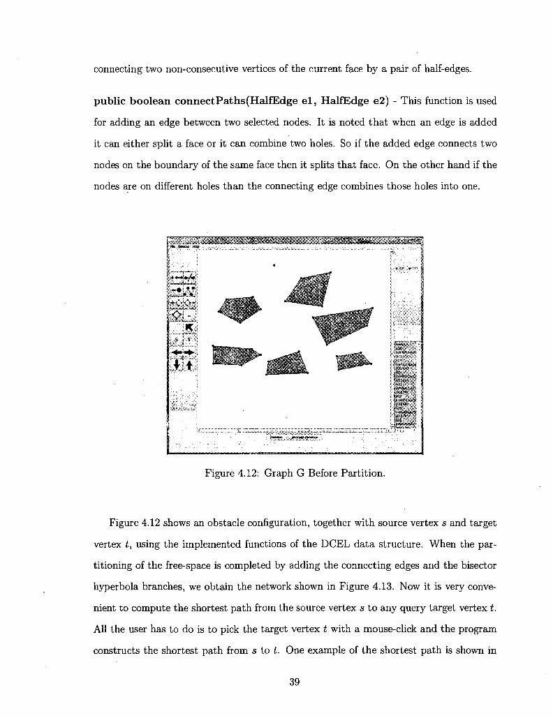
Figure 4.12: Graph G Before Partition.

Figure 4.12 shows an obstacle configuration, together with source vertex s and target

vertex t, using the implemented functions of the DCEL data structure. When the par­

titioning of the free-space is completed by adding the connecting edges and the bisector

hyperbola branches, we obtain the network shown in Figure 4.13. Now it is very conve­

nient to compute the shortest path from the source vertex s to any query target vertex t.

All the user has to do is to pick the target vertex t with a mouse-click and the program

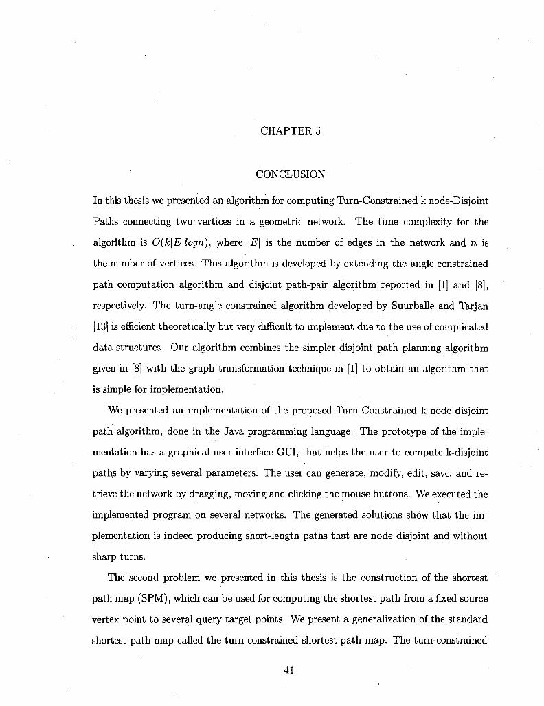
constructs the shortest path from s to t. One example of the shortest path is shown in

39

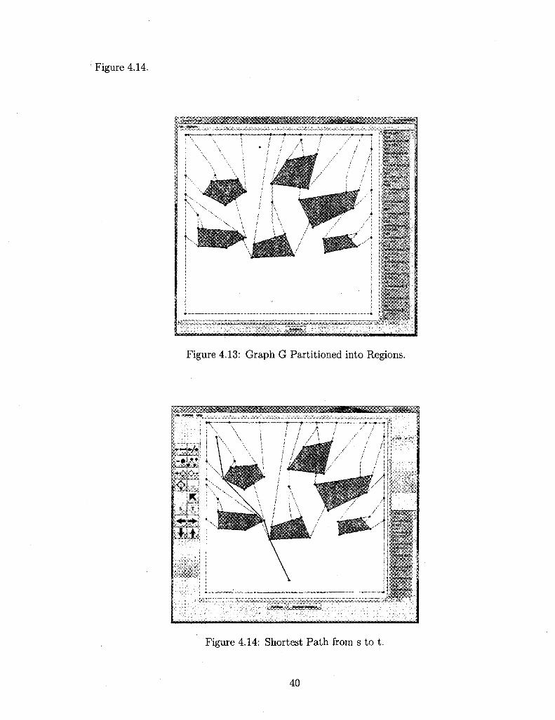
Figure 4.14.

! • ; •

** 4 i

Figure 4.13: Graph G Partitioned into Regions.

Figure 4.14: Shortest Path from s to t.

40

CHAPTER 5

CONCLUSION

In this thesis we presented an algorithm for computing Turn-Constrained k node-Disjoint

Paths connecting two vertices in a geometric network. The time complexity for the

algorithm is 0(k\E\logn), where \E\ is the number of edges in the network and n is

the number of vertices. This algorithm is developed by extending the angle constrained

path computation algorithm and disjoint path-pair algorithm reported in [1] and [8],

respectively. The turn-angle constrained algorithm developed by Suurballe and Tarjan

[13] is efficient theoretically but very difficult to implement due to the use of complicated

data structures. Our algorithm combines the simpler disjoint path planning algorithm

given in [8] with the graph transformation technique in [1] to obtain an algorithm that

is simple for implementation.

We presented an implementation of the proposed Turn-Constrained k node disjoint

path algorithm, done in the Java programming language. The prototype of the imple­

mentation has a graphical user interface GUI, that helps the user to compute k-disjoint

paths by varying several parameters. The user can generate, modify, edit, save, and re­

trieve the network by dragging, moving and clicking the mouse buttons. We executed the

implemented program on several networks. The generated solutions show that the im­

plementation is indeed producing short-length paths that are node disjoint and without

sharp turns.

The second problem we presented in this thesis is the construction of the shortest

path map (SPM), which can be used for computing the shortest path from a fixed source

vertex point to several query target points. We present a generalization of the standard

shortest path map called the turn-constrained shortest path map. The turn-constrained

41

shortest path map can be used for constructing shortest path from a fixed source vertex

s to varying query vertex q such that the generated paths do not have sharp turns.

The presented algorithm is based on the repeated construction of the visibility polygon

from the front nodes. The presented algorithm can be implemented in a straight forward

manner. In fact, we presented an implementation of a prototype program for the standard

shortest path map. The implementation of the constrained version is not complete but

is in progress.

Several extensions of the proposed algorithms can be made in the future. The turn-

constrained disjoint path algorithm presented in this thesis does produce very short length

paths. But we have not been able to prove that the path pair are of shortest total length.

It would be interesting to settle this issue.

The constrained shortest path map algorithm presented in this thesis can be used

only in the presence of polygonal obstacles in two dimensions. A natural extension

would be to look for the construction of shortest path maps in three dimensions. Since

the problem of constructing shortest path in three dimensions in known to be intractable

[2], the corresponding shortest path map construction problem in three dimensions should

be very difficult. As a first step in this direction we plan to explore the construction of

shortest path map in terrain surface which is generally viewed as two and half dimensions.

42

BIBLIOGRAPHY

[1] Ali Boroujerdi, Jeffrey Uhlmann, An efficient algorithm, for computing least cost

paths with turn constraints, Information Processing Letters 67 (1998) 317 - 321

[2] John Canny, John Reif, New Lower Bound Techniques for Robot Motion Planning

Problems, IEEE Proceedings of the 28th Annual Symposium on Foundations of

Computer Science, (1987) pp 4 9 - 6 0

[3] T. Cormen, C. Leiserson, R. Rivestam C. Stein, Introduction to Algorithms, MIT

Press and McGraw-Hill, (2001)

[4] E. W. Dijkstra, A note on Two Problems in Connection with Graphs, Numer. Math,

1 (1959) pp 269-271

[5] Jonh Hershberger, Subhash Suri, An optimal Algorithm for Euclidean Shortest Path

in the Plane, SIAM J. Comput. Vol 28 No 6 (1999) pp 2215-2256

[6] J, Krozel, C. Lee, J. S. B. Mitchell, Turn-Constrained Route Planning for Avoiding

Hazardous Weather, Air Trafic Control quarterly Vol 14(2) (2006) pp 159-182

[7] Lee D. T , Preparata F. P., Euclidean Shortest Path in the Presence of Rectilinear

Barriers, Networks Vol. 14 (1984) pp 393 - 410

[8] Daniel Mazzella, Disjoint Path in Geometric Graphs MS Thesis, School of Computer

Science Univ. of Nevada Las Vegas, (2006)

[9] Joseph S. B. Mitchell, Gunter Rote, Gerhard Woeginger Minimum-link path among

obstacles in the plane, Algorithmica, 6 (1992) pp 431-459

[10] J. O'Rourke, Computational Geometry in C, Cambridge UniversityPress 2 (1998)

43

[11] James A. Storer, John H. Reif, Shortest Path in a the Plane with Polygonal Obstacles,

Journal of ACM vol 41, No 5, September (1984) pp 983 - 1012

[12] S. Suri, J. O'rourke, Worst-case optimal algorithms for constructing visibility poly­

gons with holes, Proceedings of the second annual symposium on Computational

Geometry, (1986) pp 14-23

[13] J. W. Suurballe, R. E. Tarjan, A quick Method for Finding Shortest Pairs of Disjoint

Paths, Networks 14 (1984) pp 325-336

44

VITA

Graduate College University of Nevada, Las Vegas

Victor M. Roman

Local Address: Las Vegas, NV

Degrees: Bachelors of Science in Electronic Engineering, 1984 Northrop University

Bachelors of Science in Computer Science, 2006 University of Nevada, Las Vegas

Thesis Title: Turn Constrained Path Planning Problems

Thesis Examination Committee: Chairperson, Dr. Laxmi Gewali Ph. D. Committee Member, Dr. Jan B. Pedersen, Ph. D. Committee Member, Dr. John Minor Ph. D. Graduate Faculty Representative, Dr. Henry Selvaraj, Ph. D.

45