lecture 22 notes: probabilistic methods & optimization ... · introduction to design...

Introduction to Design Exploration: Introduction to Design Exploration:Design of Experiments Methods

16.90

5 May, 2014

Willcox, 16.90, Spring 2014 1

Today’s Topics

• Design of experiments (DOE) overview

• Some DOE methods

• Calculating effects

• Paper airplane experiment


Monte Carlo Simulation vs. Design of Experiments

• We use Monte Carlo simulation when we want to conduct a probabilistic analysis – Rigorous estimates for mean, variance,

probability of failure etc.

• Sometimes we just want to do some sampling to explore the design space, understand the “effects” of our design variables, etc. → Design of Experiments methods


Design of Experiments

• A collection of statistical techniques providing a systematic way to sample the design space

• Study the effects of multiple input variables on one or more output parameters

• Often used before setting up a formal design optimization problem

– Identify key drivers among potential design variables

– Identify appropriate design variable ranges – Identify achievable objective function values


Design of Experiments

Design variables = factors Values of design variables = levels Noise factors = variables over which we have no control

e.g., manufacturing variation in blade thickness Control factors = variables we can control

e.g., nominal blade thickness Outputs = observations (= objective functions)

Factors +

Levels “Experiment” Observation (Often an analysis code)


Matrix Experiments • Each row of the matrix corresponds to one experiment. • Each column of the matrix corresponds to one factor. • Each experiment corresponds to a different combination of

factor levels and provides one observation.

Expt No. Factor A Factor B Observation

1 A1 B1 h1

2 A1 B2 h2

3 A2 B1 h3

4 A2 B2 h4

Here, we have two factors, each of which can take two levels. Willcox, 16.90, Spring 2014

6

FullFull-Full-Factorial Experiment • Specify levels for each factor • Evaluate outputs at every combination of values n factors – complete but expensive!

ln observations

l levels

2 factors, 3 levels each:

ln = 32 = 9 expts


ln = 34 = 81 expts

Expt No.

Factor A B

1 A1 B1

2 A1 B2

3 A1 B3

4 A2 B1

5 A2 B2

6 A2 B3

7 A3 B1

8 A3 B2

9 A3 B3


Fractional Factorial Experiments

• Due to the combinatorial explosion, we cannot usually perform a full factorial experiment

• So instead we consider just some of the possible combinations

• Questions: – How many experiments do I need? – Which combination of levels should I

choose? • Need to balance experimental cost with design

space coverage


Parameter Study • Specify levels for each factor • Change one factor at a time, all others at base level • Consider each factor at every level

n factors

9

l levels


1+n(l-1) =

1+4(3-1) = 9 expts

1+n(l-1) evaluations

Expt No.

Factor A B C D

1 A1 B1 C1 D1

2 A2 B1 C1 D1

3 A3 B1 C1 D1

4 A1 B2 C1 D1

5 A1 B3 C1 D1

6 A1 B1 C2 D1

7 A1 B1 C3 D1

8 A1 B1 C1 D2

9 A1 B1 C1 D3

Baseline : A1, B1, C1, D1

Willcox, 16.90, Spring 2014

Parameter Study • Select the best result for each factor

Expt No.

Factor Observation

A B C D

1 A1 B1 C1 D1 h1

2 A2 B1 C1 D1 h2

3 A3 B1 C1 D1 h3

4 A1 B2 C1 D1 h4

5 A1 B3 C1 D1 h5

6 A1 B1 C2 D1 h6

7 A1 B1 C3 D1 h7

8 A1 B1 C1 D2 h8

9 A1 B1 C1 D3 h9

1. Compare h , h , h1 2 3

A*

2. Compare h1, h4, h5

B*

3. Compare h1, h6, h7

C*

4. Compare h , h , h1 8 9

D*

“Good design” is A*,B*,C*,D*

• Limitations?


One At a Time Change first factor, all others at base value

n factors

l levels

1+n(l-1) evaluations

•

• If output is improved, keep new level for that factor • Move on to next factor and repeat


1+n(l-1) =

1+4(3-1) = 9 expts

Expt No.

Factor A B C D

1 A1 B1 C1 D1

2 A2 B1 C1 D1

3 A3 B1 C1 D1

4 A* B2 C1 D1

5 A* B3 C1 D1

6 A* B* C2 D1

7 A* B* C3 D1

8 A* B* C* D2

9 A* B* C* D3

• Limitations? 11


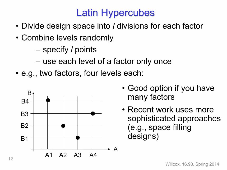
Latin Hypercubes • Divide design space into l divisions for each factor • Combine levels randomly

– specify l points – use each level of a factor only once

• e.g., two factors, four levels each:

• Good option if you havemany factors

• Recent work uses more sophisticated approaches(e.g., space filling designs)

A A1 A2 A3 A4

B

B1

B2

B3

B4


Orthogonal Arrays

• Specify levels for each factor • Use arrays to choose a subset of the full-

factorial experiment • Subset selected to maintain “orthogonality”

between factors

n factors

l levels subset of ln evaluations

• Does not capture all interactions, but can be efficient

• Experiment is balanced


Orthogonal Arrays

Expt No.

Factor

A B C

1 A1 B1 C1

2 A1 B2 C2

3 A2 B1 C2

4 A2 B2 C1

L (23)4

4 expts 3 factors L9(34) 2 levels

9 expts 4 factors 3 levels

Expt No.

Factor

A B C D

1 A1 B1 C1 D1

2 A1 B2 C2 D2

3 A1 B3 C3 D3

4 A2 B1 C2 D3

5 A2 B2 C3 D1

6 A2 B3 C1 D2

7 A3 B1 C3 D2

8 A3 B2 C1 D3

9 A3 B3 C2 D1


Effects

Once the experiments have been performed, the results can be used to calculate effects.

The effect of a factor is the change in the response as the level of the factor is changed.

– Main effects: averaged individual measures of effects of factors

– Interaction effects: the effect of a factor depends on the level of another factor

Often, the effect is determined for a change from a minus level (-) to a plus level (+) (2-level experiments).


Effects

Consider the following experiment: –We are studying the effect of three factors on the price of

an aircraft –The factors are the number of seats, range and aircraft

manufacturer – Each factor can take two levels:

Factor 1: Seats 100<S1<150 150<S2<200

Factor 2: Range (nm) 2000<R1<2800 2800<R2<3500

Factor 3: Manufacturer M1=Boeing M2=Airbus


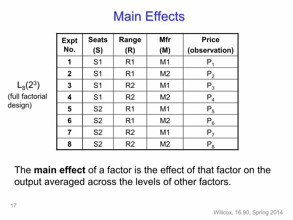
Main Effects

L8(23) (full factorial design)

Expt No.

Seats (S)

Range (R)

Mfr (M)

Price (observation)

1 S1 R1 M1 P1

2 S1 R1 M2 P2

3 S1 R2 M1 P3

4 S1 R2 M2 P4

5 S2 R1 M1 P5

6 S2 R1 M2 P6

7 S2 R2 M1 P7

8 S2 R2 M2 P8

The main effect of a factor is the effect of that factor on the output averaged across the levels of other factors.


Main Effects Question: what is the main effect of manufacturer? i.e., from our experiments, can we estimate how the price is affected by whether Boeing or Airbus makes the aircraft (averaged across range and seats)?

Expt No.

Seats (S)

Range (R)

Mfr (M)

Price (observation)

1 S1 R1 M1 P1

2 S1 R1 M2 P2

3 S1 R2 M1 P3

4 S1 R2 M2 P4

5 S2 R1 M1 P5

6 S2 R1 M2 P6

7 S2 R2 M1 P7

8 S2 R2 M2 P8


Computing the main effect of manufacturer P1 P2 3+ P P4+ +P P5 6 P7 P m 8

8 overall mean

response:

avg over all expts P1 P P5 P when M=M1 : mM1 3

4 7

effect of mfr = level M1

m mM1 effect of mfr =

level M2 m mM 2

Effect of factor level can be defined for multiple levels

main effect of mfr = 2 1M Mm m Main effect of factor is defined as

difference between two levels

NOTE: The main effect should be interpreted individually only if the variable does not appear to interact with other variables


Main Effect Example Expt Seats Range Mfr Price

Aircraft No. (S) (R) (M) ($M) 1 717 S1 R1 M1 24.0 2 A318-100 S1 R1 M2 29.3 3 737-700 S1 R2 M1 33.0 4 A319-100 S1 R2 M2 35.0 5 737-900 S2 R1 M1 43.7 6 A321-200 S2 R1 M2 48.0 7 737-800 S2 R2 M1 39.1 8 A320-200 S2 R2 M2 38.0

100<S1<150 150<S2<200 2000<R1<2800 2800<R2<3500 M1=Boeing M2=Airbus

Sources: Seats/Range data: Boeing Quick Looks Price data: Aircraft Value News Airline Monitor, May 2001 issue


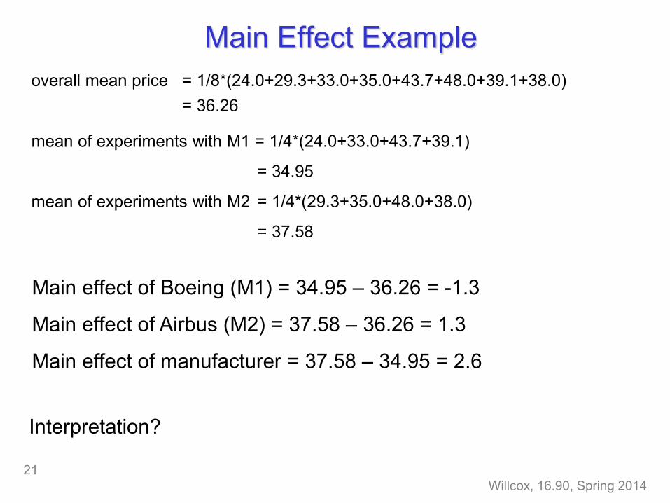
Main Effect Example = 1/8*(24.0+29.3+33.0+35.0+43.7+48.0+39.1+38.0) = 36.26

overall mean price

mean of experiments with M1 = 1/4*(24.0+33.0+43.7+39.1)

= 34.95

mean of experiments with M2 = 1/4*(29.3+35.0+48.0+38.0)

= 37.58

Main effect of Boeing (M1) = 34.95 – 36.26 = -1.3

Main effect of Airbus (M2) = 37.58 – 36.26 = 1.3

Main effect of manufacturer = 37.58 – 34.95 = 2.6

Interpretation?


Interaction Effects We can also measure interaction effects between factors. Answers the question: does the effect of a factor depend on the level of another factor?

e.g., Does the effect of manufacturer depend on whether we consider shorter range or longer range aircraft?

The interaction between manufacturer and range is defined as half the difference between the average manufacturer effect with range 2 and the average manufacturer effect with range 1.

avg mfr effect avg mfr effect mfr range -with range 2 with range 1 =interaction 2


range R1 : expts 1,2,5,6

range R2 : expts 3,4,7,8

Interaction Effects Expt Seats Range Mfr Price No. (S) (R) (M) ($M)

1 S1 R1 M1 24.0

2 S1 R1 M2 29.3

3 S1 R2 M1 33.0

4 S1 R2 M2 35.0

5 S2 R1 M1 43.7

6 S2 R1 M2 48.0

7 S2 R2 M1 39.1

8 S2 R2 M2 38.0

(P P2 1 - )+ (P6 -P5 ) 2

avg mfr effect with range 1

(29.3-24.0)+ (48.0-43.7) 4.8

2

avg mfr effect with range 2

(P4 3- )P + ( -P P8 7 ) 2

(35.0-33.0)+ (38.0-39.1) 0.45

2

23

mfr range interaction

0.45 4.8 2.2

2 Interpretation?


Interpretation of Effects Main effects are the difference between two

averages

seats range

manufacturer

seats

range

mfr

S2S1

1

2

3

4

5

6

7

8

R1

R2

1

2

3

4

5

6

7

8

M2

M1

1

2

3

4

5

6

7

8

main effect of mfr

Expt No.

Seats (S)

Range (R)

Mfr (M)

1 S1 R1 M1

2 S1 R1 M2

3 S1 R2 M1

4 S1 R2 M2

5 S2 R1 M1

6 S2 R1 M2

7 S2 R2 M1

8 S2 R2 M2

8 6 4 2 7 5 3 1( + + + )-( + + + ) 4

P P P P P P P P

Willcox, 16.90, Spring 2014 from Fig 10.2 Box, Hunter & Hunter

24

range Interaction effects are

also the difference between two averages, seats but the planes are no

mfr longer parallel

Interpretation of Effects Expt Seats Range Mfr No. (S) (R) (M)

1 S1 R1 M1

2 S1 R1 M2

3 S1 R2 M1

4 S1 R2 M2

5 S2 R1 M1

6 S2 R1 M2

7 S2 R2 M1

8 S2 R2 M2

1

2

3

4

5

6

7

8

1

2

3

4

5

6

7

8

1

2

3

4

5

6

7

8

seats range mfr seats

(P P P+ + P )-( P P + + )+ + P Pmfr range 8 5 4 1 7 6 3 2 interaction

4

from Fig 10.2 Box, Hunter & Hunter

mfr range


Design Experiment

Objective: Maximize Airplane Glide Distance

Design Variables: Weight Distribution Stabilizer Orientation Nose Length Wing Angle

Three levels for each design variable. Experiment courtesy of Prof. Eppinger


Design Experiment Full factorial design : 34=81 experiments

We will use an L9(34) orthogonal array:

Expt No.

Weight A

Stabilizer B

Nose C

Wing D

1 A1 B1 C1 D1 2 A1 B2 C2 D2 3 A1 B3 C3 D3 4 A2 B1 C2 D3 5 A2 B2 C3 D1 6 A2 B3 C1 D2 7 A3 B1 C3 D2 8 A3 B2 C1 D3 9 A3 B3 C2 D1


Design Experiment Things to think about ...

Given just 9 out of a possible 81 experiments, can we predict the optimal airplane?

Do some design variables seem to have a larger effect on the objective than others (sensitivity)?

Are there other factors affecting the results (noise)?


MIT OpenCourseWarehttp://ocw.mit.edu

16.90 Computational Methods in Aerospace Engineering Spring 2014

For information about citing these materials or our Terms of Use, visit: http://ocw.mit.edu/terms.

http://ocw.mit.edu

http://ocw.mit.edu/terms

lecture 22 notes: probabilistic methods & optimization ... · introduction to design...

Documents