Lecture 14: Thur., Feb. 26

• Multiple Comparisons (Sections 6.3-6.4)

• Next class: Inferences about Linear Combinations of Group Means (Section 6.2).

Discrimination against the Handicapped (Case Study 6.1)

• Study of how physical handicaps affect people’s perception of employment qualifications.

• Researchers prepared five videotaped job interviews, using same two male actors for each. Tapes differed only in that applicant appeared with a different handicap in each– (i) wheelchair; (ii) on crutches; (iii) hearing impaired; (iv) one leg amputated; (v) no handicap.

• Each tape shown to 14 students from U.S. university. Students rate qualifications of candidate on 0 to 10 point scale based on tape.

• Questions of interest: Do subjects systematically evaluate qualifications differently according to candidate’s handicap? If so, which handicaps produce different evaluations?

O n e w a y A n a l y s i s o f S C O R E B y H A N D I C A P

SCOR

E

1

34

6

8

AMPUTEECRUTCHES

HEARINGNONE

WHEELCHAIR

HANDICAP

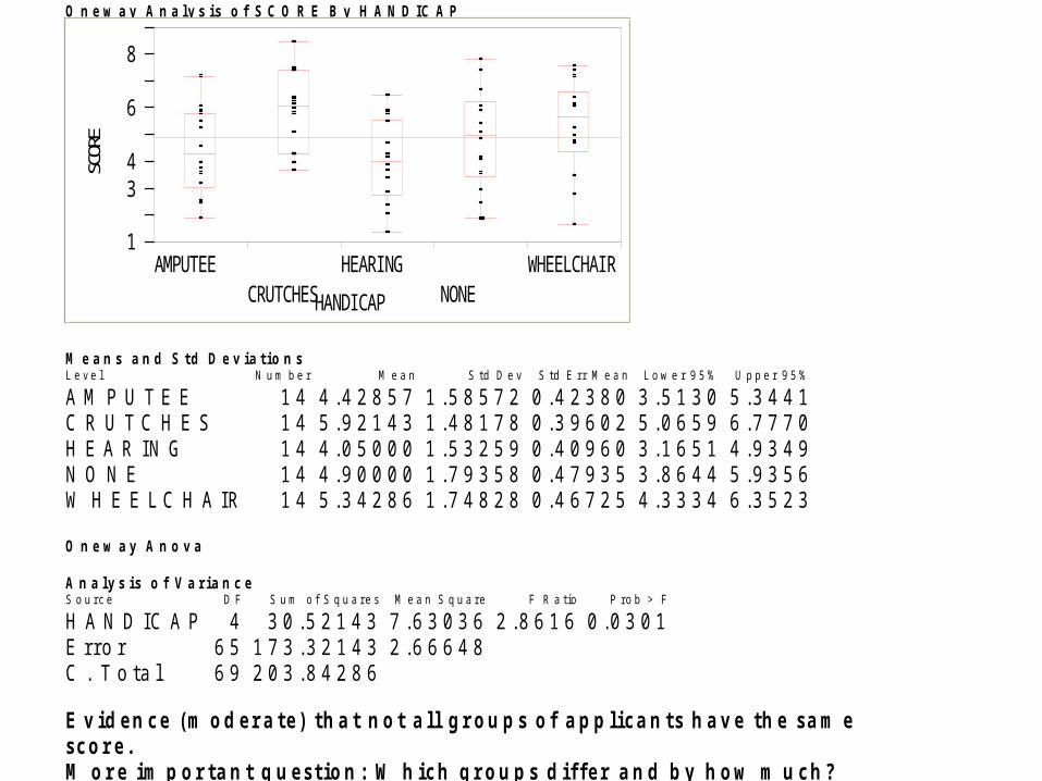
M e a n s a n d S t d D e v i a t i o n s L e v e l N u m b e r M e a n S t d D e v S t d E r r M e a n L o w e r 9 5 % U p p e r 9 5 %

A M P U T E E 1 4 4 . 4 2 8 5 7 1 . 5 8 5 7 2 0 . 4 2 3 8 0 3 . 5 1 3 0 5 . 3 4 4 1 C R U T C H E S 1 4 5 . 9 2 1 4 3 1 . 4 8 1 7 8 0 . 3 9 6 0 2 5 . 0 6 5 9 6 . 7 7 7 0 H E A R I N G 1 4 4 . 0 5 0 0 0 1 . 5 3 2 5 9 0 . 4 0 9 6 0 3 . 1 6 5 1 4 . 9 3 4 9 N O N E 1 4 4 . 9 0 0 0 0 1 . 7 9 3 5 8 0 . 4 7 9 3 5 3 . 8 6 4 4 5 . 9 3 5 6 W H E E L C H A I R 1 4 5 . 3 4 2 8 6 1 . 7 4 8 2 8 0 . 4 6 7 2 5 4 . 3 3 3 4 6 . 3 5 2 3 O n e w a y A n o v a A n a l y s i s o f V a r i a n c e S o u r c e D F S u m o f S q u a r e s M e a n S q u a r e F R a t i o P r o b > F

H A N D I C A P 4 3 0 . 5 2 1 4 3 7 . 6 3 0 3 6 2 . 8 6 1 6 0 . 0 3 0 1 E r r o r 6 5 1 7 3 . 3 2 1 4 3 2 . 6 6 6 4 8 C . T o t a l 6 9 2 0 3 . 8 4 2 8 6 E v i d e n c e ( m o d e r a t e ) t h a t n o t a l l g r o u p s o f a p p l i c a n t s h a v e t h e s a m e s c o r e . M o r e i m p o r t a n t q u e s t i o n : W h i c h g r o u p s d i f f e r a n d b y h o w m u c h ?

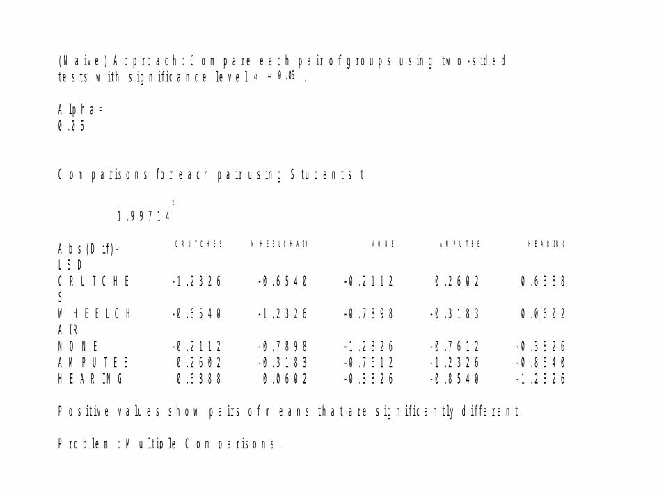
( N a i v e ) A p p r o a c h : C o m p a r e e a c h p a i r o f g r o u p s u s i n g t w o - s i d e d t e s t s w i t h s i g n i f i c a n c e l e v e l 05.0 . A l p h a = 0 . 0 5 C o m p a r i s o n s f o r e a c h p a i r u s i n g S t u d e n t ' s t

t

1 . 9 9 7 1 4 A b s ( D i f ) -L S D

C R U T C H E S W H E E L C H A I R N O N E A M P U T E E H E A R I N G

C R U T C H ES

- 1 . 2 3 2 6 - 0 . 6 5 4 0 - 0 . 2 1 1 2 0 . 2 6 0 2 0 . 6 3 8 8

W H E E L C HA I R

- 0 . 6 5 4 0 - 1 . 2 3 2 6 - 0 . 7 8 9 8 - 0 . 3 1 8 3 0 . 0 6 0 2

N O N E - 0 . 2 1 1 2 - 0 . 7 8 9 8 - 1 . 2 3 2 6 - 0 . 7 6 1 2 - 0 . 3 8 2 6 A M P U T E E 0 . 2 6 0 2 - 0 . 3 1 8 3 - 0 . 7 6 1 2 - 1 . 2 3 2 6 - 0 . 8 5 4 0 H E A R I N G 0 . 6 3 8 8 0 . 0 6 0 2 - 0 . 3 8 2 6 - 0 . 8 5 4 0 - 1 . 2 3 2 6 P o s i t i v e v a l u e s s h o w p a i r s o f m e a n s t h a t a r e s i g n i f i c a n t l y d i f f e r e n t . P r o b l e m : M u l t i p l e C o m p a r i s o n s .

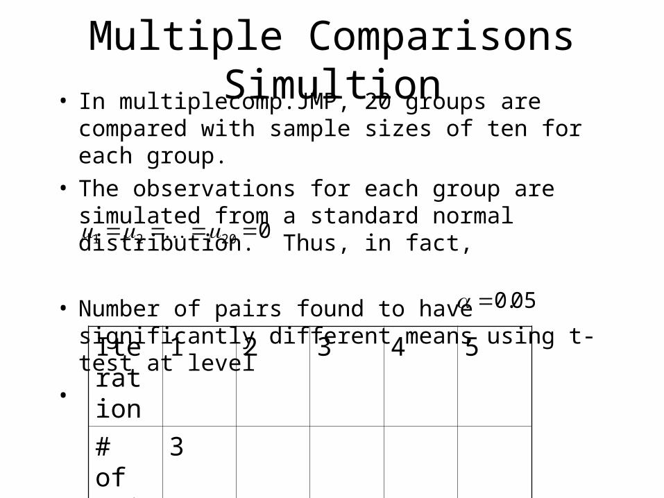
Multiple Comparisons Simultion• In multiplecomp.JMP, 20 groups are compared

with sample sizes of ten for each group.• The observations for each group are simulated

from a standard normal distribution. Thus, in fact,

• Number of pairs found to have significantly

different means using t-test at level•

02021

05.0

Iteration

1 2 3 4 5

# of Pairs

3

Compound Uncertainty

• Compound uncertainty: When drawing more than one direct inference, there is an increased chance of making at least one mistake.

• Impact on tests: If using a conventional criteria such as a p-value of 0.05 to reject a null hypothesis, the probability of falsely rejecting at least one null hypothesis will be greater than 0.05 if considering multiple tests.

• Impact on confidence intervals: If forming multiple 95% confidence intervals, the chance that all of the confidence intervals will contain true parameter is less than 95%.

Simultaneous Inferences

• When several tests are considered simultaneously, they constitute a family of tests.

• Individual Type I error rate: Probability for a single test that the null hypothesis will be rejected assuming that the null hypothesis is true.

• Familywise Type I error rate: Probability for a family of test that at least one null hypothesis will be rejected assuming that all of the null hypotheses are true.

Individual vs. Family Confidence Levels

• If a family consists of k tests, each with individual type I error rate 0.05, the familywise type I error rate is at least 0.05 and no larger than k*0.05.

• Actual familywise type I error rate depends on degree of dependence between tests.

• If the tests are independent, the familywise type I error rate is 1-(.95)k

• If all the null hypotheses in a family true, the mean number of Type I errors equals k*0.05.

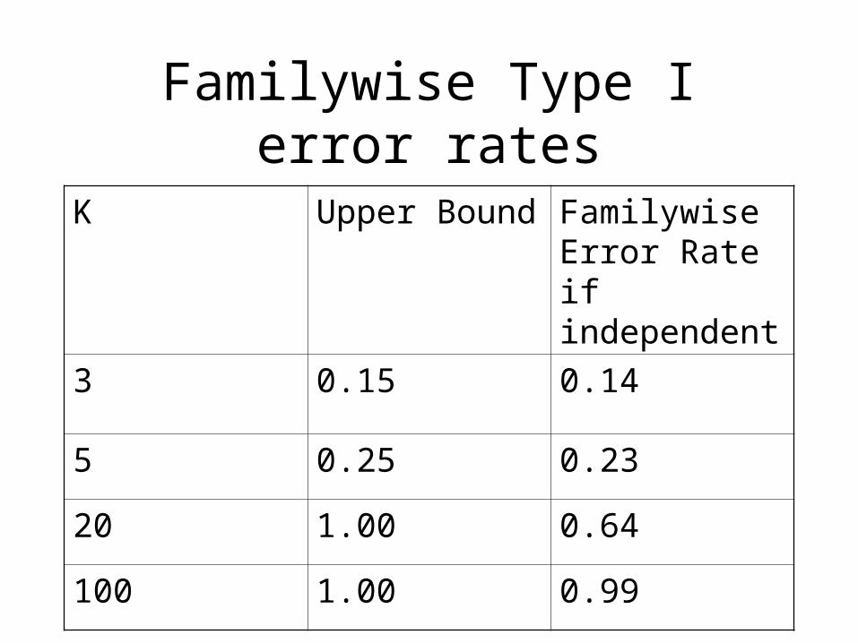
Familywise Type I error rates

K Upper Bound Familywise Error Rate if independent

3 0.15 0.14

5 0.25 0.23

20 1.00 0.64

100 1.00 0.99

Multiple Comparison Procedures

• Multiple comparison procedures are methods of carrying out tests so that the familywise type I error rate is controlled (at 0.05 for example).

• Key issue: What is the appropriate family to consider?

Planned vs. Unplanned Comparisons• Consider one-way layout with 20 groups.• Planned Comparisons: researcher is specifically

interested in comparing groups 1 and 4 because comparison answers a research question directly. This is a planned comparison. In the mice diets example, the researchers had five planned comparisons.

• Unplanned Comparisons: researcher examines all possible pairs of groups – 190 groups. As a result, researcher finds that only groups 5 and 8 suggest actual differences. Only this pair is reported as significant. For the handicap example, the comparisons were unplanned.

Families in Planned/Unplanned

• Planned Comparisons: The family of tests is the family of all planned comparisons (e.g., the family of five planned comparisons in mice diet). For small number of planned comparisons, it is usual practice to just use individual type I error rates.

• Unplanned Comparisons: The family of tests is the family of all possible comparisons - (k*(k-1)/2) for a k-group one-way layout. It is important to control the familywise type I error rate for unplanned comparisons. The handicap study involves unplanned comparisons.

Multiple Comparisons Procedures

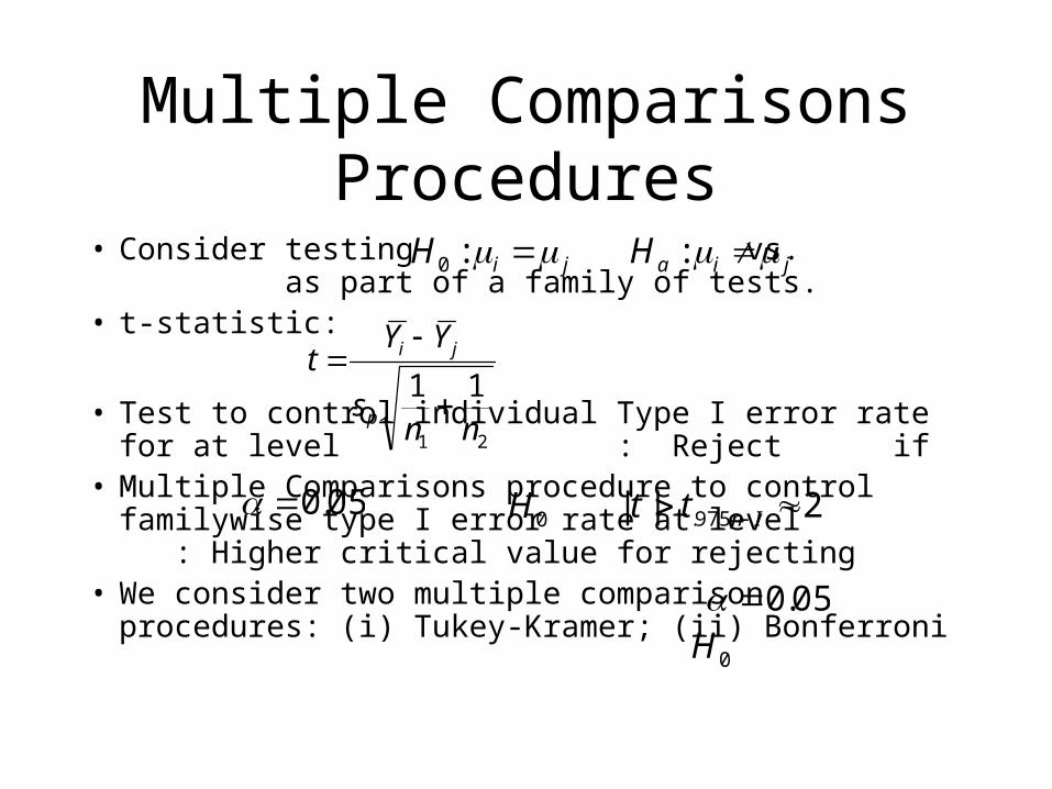
• Consider testing vs. as part of a family of tests.

• t-statistic:

• Test to control individual Type I error rate for at level : Reject if

• Multiple Comparisons procedure to control familywise type I error rate at level : Higher critical value for rejecting

• We consider two multiple comparison procedures: (i) Tukey-Kramer; (ii) Bonferroni

21

11nn

s

YYt

p

ji

jiH :0 jiaH :

05.00H 2|| ,975. Intt

05.00H

Tukey-Kramer

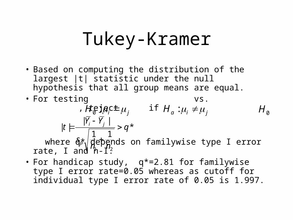
• Based on computing the distribution of the largest |t| statistic under the null hypothesis that all group means are equal.

• For testing vs. , reject if

where q* depends on familywise type I error rate, I and n-I.

• For handicap study, q*=2.81 for familywise type I error rate=0.05 whereas as cutoff for individual type I error rate of 0.05 is 1.997.

jiH :0 jiaH : 0H

*11

||||

21

q

nns

YYt

p

ji

Tukey-Kramer in JMP

• To see which groups are significantly different (in sense of statistical significance) at a familywise Type I error rate of 0.05, click Compare Means under Oneway Analysis (after Analyze, Fit Y by X) and click All Pairs, Tukey’s HSD.

• In table “Comparison of All Pairs Using Tukey’s HSD,” two groups are significantly different if and only if the entry in the table for the pair of groups is positive.

• The cutoff value q* is listed in the output.

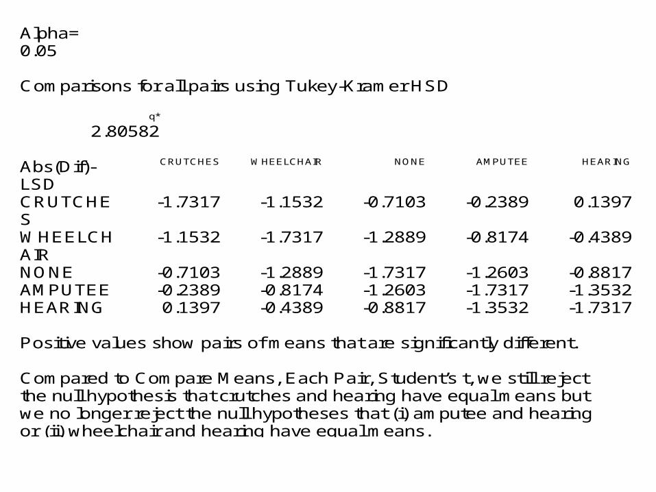
Alpha= 0.05 Comparisons for all pairs using Tukey-Kramer HSD

q*

2.80582 Abs(Dif)-LSD

CRUTCHES WHEELCHAIR NONE AMPUTEE HEARING

CRUTCHES

-1.7317 -1.1532 -0.7103 -0.2389 0.1397

WHEELCHAIR

-1.1532 -1.7317 -1.2889 -0.8174 -0.4389

NONE -0.7103 -1.2889 -1.7317 -1.2603 -0.8817 AMPUTEE -0.2389 -0.8174 -1.2603 -1.7317 -1.3532 HEARING 0.1397 -0.4389 -0.8817 -1.3532 -1.7317 Positive values show pairs of means that are significantly different. Compared to Compare Means, Each Pair, Student’s t, we still reject the null hypothesis that crutches and hearing have equal means but we no longer reject the null hypotheses that (i) amputee and hearing or (ii) wheelchair and hearing have equal means.

Bonferroni Method

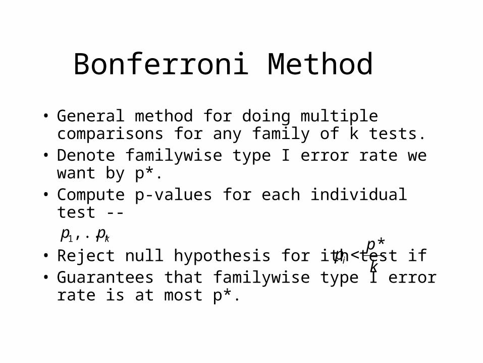
• General method for doing multiple comparisons for any family of k tests.

• Denote familywise type I error rate we want by p*.

• Compute p-values for each individual test -- • Reject null hypothesis for ith test if• Guarantees that familywise type I error rate is at

most p*.

kpp ,...,1

k

ppi

*

Bonferroni for mice diets

• Five comparisons were planned. Suppose we want the familywise error rate for the five comparisons to be 0.05.

• Bonferroni method: We should consider two groups to be significantly different if the p-value from the two-sided t-test is less than 0.05/5=0.01.

• Bonferroni in JMP: To do each test at a given level, after Fit Y by X, click red triangle next to Oneway Analysis and click Set Alpha Level. Then click Compare Means and Each Pair, Student’s t. This will show results of tests at chosen alpha level.

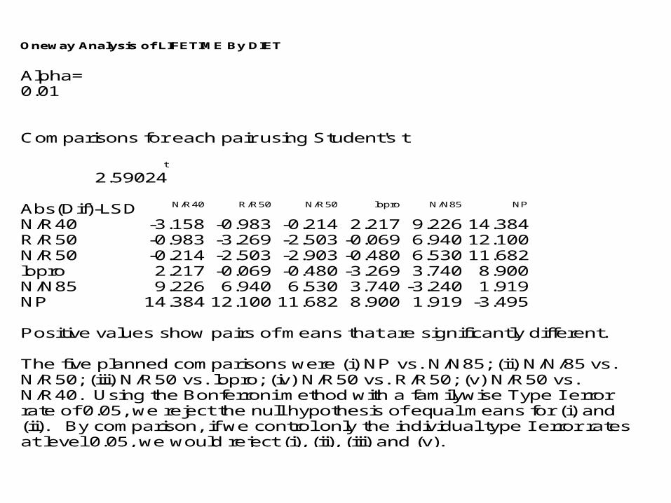
Oneway Analysis of LIFETIME By DIET

Alpha= 0.01 Comparisons for each pair using Student's t

t

2.59024 Abs(Dif)-LSD

N/R40 R/R50 N/R50 lopro N/N85 NP

N/R40 -3.158 -0.983 -0.214 2.217 9.226 14.384 R/R50 -0.983 -3.269 -2.503 -0.069 6.940 12.100 N/R50 -0.214 -2.503 -2.903 -0.480 6.530 11.682 lopro 2.217 -0.069 -0.480 -3.269 3.740 8.900 N/N85 9.226 6.940 6.530 3.740 -3.240 1.919 NP 14.384 12.100 11.682 8.900 1.919 -3.495 Positive values show pairs of means that are significantly different. The five planned comparisons were (i) NP vs. N/N85; (ii) N/N/85 vs. N/R50; (iii) N/R50 vs. lopro; (iv) N/R50 vs. R/R50; (v) N/R50 vs. N/R40. Using the Bonferroni method with a familywise Type I error rate of 0.05, we reject the null hypothesis of equal means for (i) and (ii). By comparison, if we control only the individual type I error rates at level 0.05, we would reject (i), (ii), (iii) and (v).

Multiple Comparisons and Confidence Intervals

• When several 95% confidence intervals are considered simultaneously, they constitute a family of confidence intervals

• Individual Confidence Level: Success rate of a procedure for constructing a single confidence interval.

• Familywise Confidence Level: Success rate of procedure for constructing a family of confidence intervals, where a “successful” usage is one in which all intervals in the family capture their parameters.

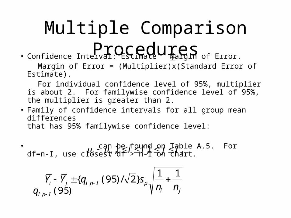
Multiple Comparison Procedures• Confidence Interval: Estimate Margin of Error. Margin of Error = (Multiplier)x(Standard Error of Estimate). For individual confidence level of 95%, multiplier is about 2. For

familywise confidence level of 95%, the multiplier is greater than 2.

• Family of confidence intervals for all group mean differences that has 95% familywise confidence level:

• can be found on Table A.5. For df=n-I, use closest df >

n-I on chart.

,1,1, IjIiji

jipInIji nnsqYY

11}2/)95(.{ ,

)95(., InIq

Multiplicity• A news report says, “A 15 year study of more than 45,000 Swedish

solidiers revealed that heavy users of marijuana were six times more likely than nonusers to develop schizophrenia.”

• Were the investigators only looking for difference in schizophrenia among heavy/non-heavy users of marijuana?

• Key question: What is their family of tests? If they were actually looking for a difference among 100 outcomes (e.g., blood pressure, lung cancer), Bonferroni should be used to control the familywise Type I error rate, i.e., only consider a difference significant if p-value is less than .05/100=.0005.

• The best way to deal with the multiple comparisons problem is to design a study to search specifically for a pattern that was suggested by an exploratory data analysis. In other words we convert an “unplanned” comparison into a “planned” comparison by doing a new experiment.