LECTURE 13:DIMENSIONALITY REDUCTIONOctober 25, 2017SDS 293: Machine Learning

Outline

• Model selection: alternatives to least-squaresüSubset selection

üBest subsetüStepwise selection (forward and backward)üEstimating error using cross-validation

üShrinkage methodsüRidge regression and the Lasso- Dimension reduction

• Labs for each part

Recap: Ridge Regression and the Lasso

• Both are “shrinkage” methods• Estimates for the coefficients are biased toward the origin- Biased = “prefers some estimates to others”- Does not yield the true value in expectation

• Question: why would we want a biased estimate?

&73?M*'&AGC7'&7C87HHA5B'?BG'4@7'!?HH5

F L54@'?87'TH@8ABQ?C7U'S74@5GHF "H4AS?47H'P58'4@7'357PPA3A7B4H'?87'!"#$%& 45N?8G'4@7'58ACAB- LA?H7G'V'TM87P78H'H5S7'7H4AS?47H'45'54@78HU- +57H'B54'WA7EG'4@7'48D7'I?ED7'AB'7XM734?4A5B

F YD7H4A5B*'N@W'N5DEG'N7'./%- ?'6A?H7G'7H4AS?47Z

What’s wrong with bias?

• What if your unbiased estimator gives you this?

May want to bias our estimate to reduce variance

i1 2 3

i

-4,000,000,000

-2,000,000,000

0

2,000,000,000

4,000,000,000

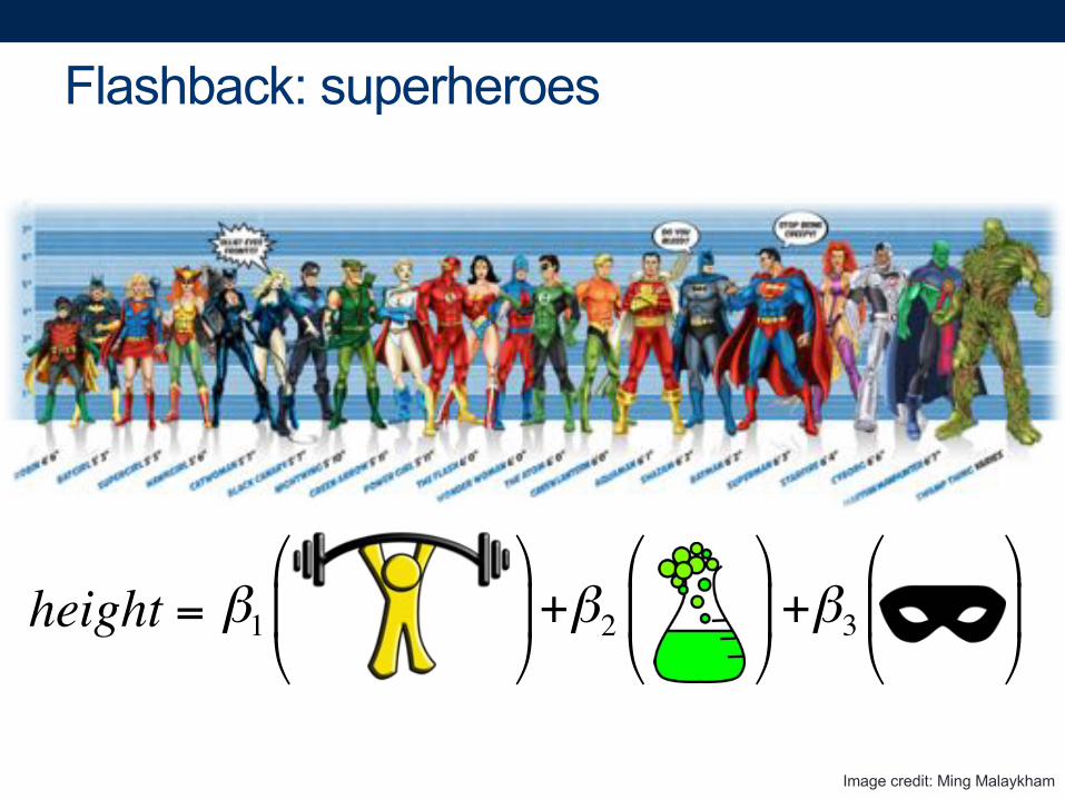
Flashback: superheroes

Image credit: Ming Malaykham

β1⎛

⎝⎜

⎞

⎠⎟height = +β2

⎛

⎝⎜

⎞

⎠⎟+β3

⎛

⎝⎜

⎞

⎠⎟

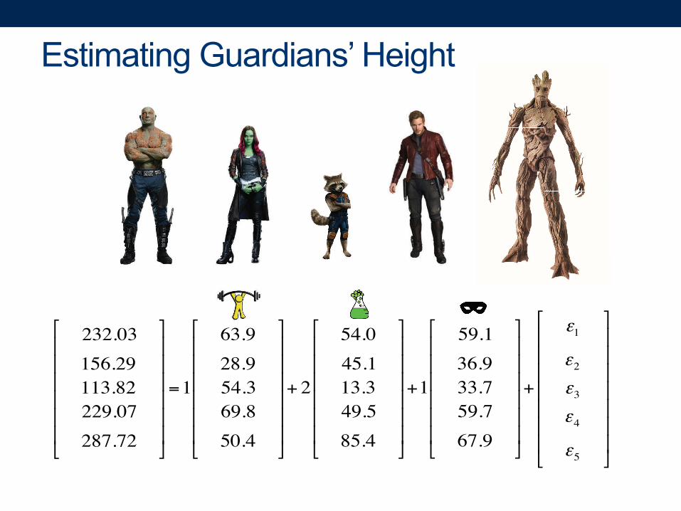
Estimating Guardians’ Height

232.03156.29113.82229.07287.72

⎡

⎣

⎢⎢⎢⎢⎢⎢

⎤

⎦

⎥⎥⎥⎥⎥⎥

=1

63.928.954.369.850.4

⎡

⎣

⎢⎢⎢⎢⎢⎢

⎤

⎦

⎥⎥⎥⎥⎥⎥

+ 2

54.045.113.349.585.4

⎡

⎣

⎢⎢⎢⎢⎢⎢

⎤

⎦

⎥⎥⎥⎥⎥⎥

+1

59.136.933.759.767.9

⎡

⎣

⎢⎢⎢⎢⎢⎢

⎤

⎦

⎥⎥⎥⎥⎥⎥

+

ε1

ε2ε3ε4

ε5

⎡

⎣

⎢⎢⎢⎢⎢⎢⎢

⎤

⎦

⎥⎥⎥⎥⎥⎥⎥

Estimate for b

• When we try to estimate using OLS, we get the following:

(Relatively) huge difference between actual and estimated coefficients

i

i

-2

0

2

4

6 estimatedtrue

≈ "#$ ,

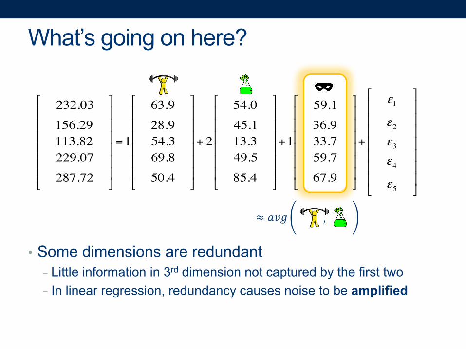
• Some dimensions are redundant- Little information in 3rd dimension not captured by the first two- In linear regression, redundancy causes noise to be amplified

232.03156.29113.82229.07287.72

⎡

⎣

⎢⎢⎢⎢⎢⎢

⎤

⎦

⎥⎥⎥⎥⎥⎥

=1

63.928.954.369.850.4

⎡

⎣

⎢⎢⎢⎢⎢⎢

⎤

⎦

⎥⎥⎥⎥⎥⎥

+ 2

54.045.113.349.585.4

⎡

⎣

⎢⎢⎢⎢⎢⎢

⎤

⎦

⎥⎥⎥⎥⎥⎥

+1

59.136.933.759.767.9

⎡

⎣

⎢⎢⎢⎢⎢⎢

⎤

⎦

⎥⎥⎥⎥⎥⎥

+

ε1

ε2ε3ε4

ε5

⎡

⎣

⎢⎢⎢⎢⎢⎢⎢

⎤

⎦

⎥⎥⎥⎥⎥⎥⎥

What’s going on here?

Dimension reduction

• Current situation: our data live in p-dimensional space, but not all p dimensions are equally useful

• Subset selection: throw some out- Pro: pretty easy to do- Con: lose some information

• Alternate approach: create new features that are combinations of the old ones

In other words: Project the data into a new feature space

to reduce variance in the estimate

Projection

Projection

Projection

Dimension reduction via projection

• Big idea: transform the data before performing regression

&' &( &) &* &+ ↦ -' -(

• Then instead of:

. = 01 +304&4

5

46'

+ 7

we solve:

. = 81 +384-4 +

9

46'

7

Linear projection

• New features are linear combinations of original data:

-: =384:&4

9

4

• MTH211: multiplying the data matrix by a projection matrix

-' -( = &' &( &) &* &+

;','

;(,'

;',(

;(,(

;),'

;*,'

;+,'

;),(

;*,(

;+,(

What’s the deal with projection?

• Data can be rotated, scaled, and translated without changing the underlying relationships

• This means you’re allowed to look at the data from whatever angle makes your life easier…

Flashback: why did we pick this line?

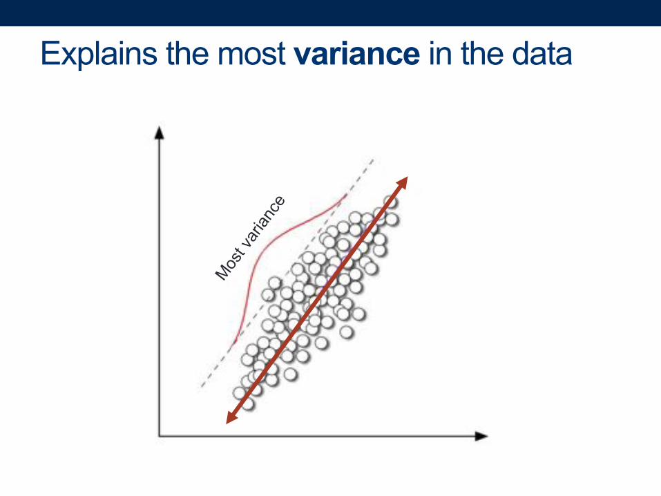
Explains the most variance in the data

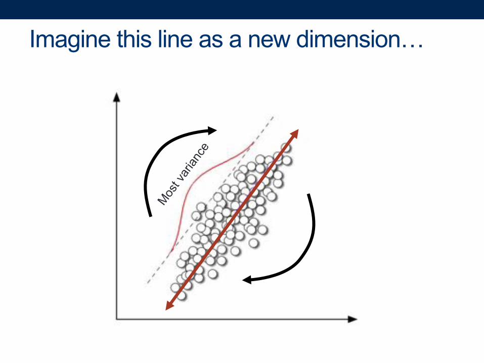
Imagine this line as a new dimension…

“Principal component”

Mathematically

• The 1st principal component is the normalized* linear combination of features:

-' = <''&' + <('&( +⋯+ <5'&5

that has the largest variance

• <'',… , <5': the loadings of the 1st principal component

* By normalized we mean: 3<:'

(= 1

5

:6'

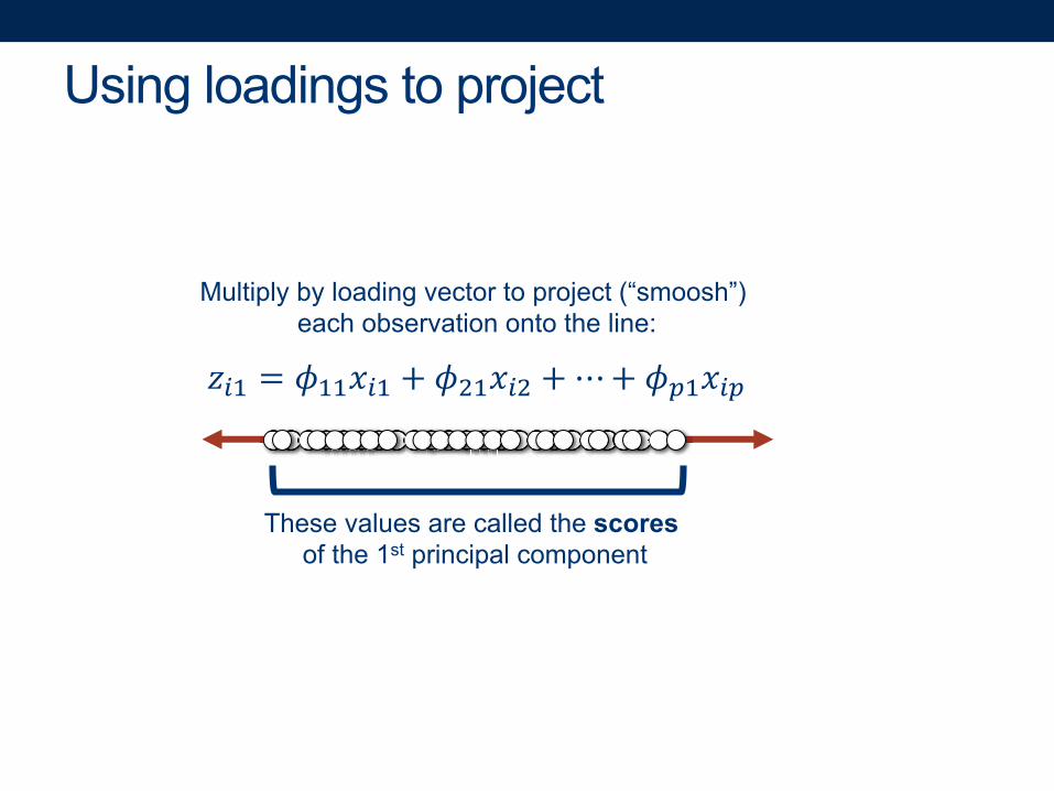
Using loadings to project

Multiply by loading vector to project (“smoosh”) each observation onto the line:

@4' = <''A4' + <('A4( + ⋯+ <5'A45

These values are called the scoresof the 1st principal component

Additional principal components

• 2nd principal component is the normalized linear combination of the features

-( = <'(&' + <((&( +⋯+ <5(&5

that has maximal variance out of all linear combinations that are uncorrelated with Z1 (why does that matter?)

• Fun fact:

Principal components are orthogonal

Generating additional principal components

• We can think of this recursively• To find the BCℎ principal component . . .- Find the first (B − 1)principal components- Subtract the projection into that space-Maximize the variance in the remaining complementary space

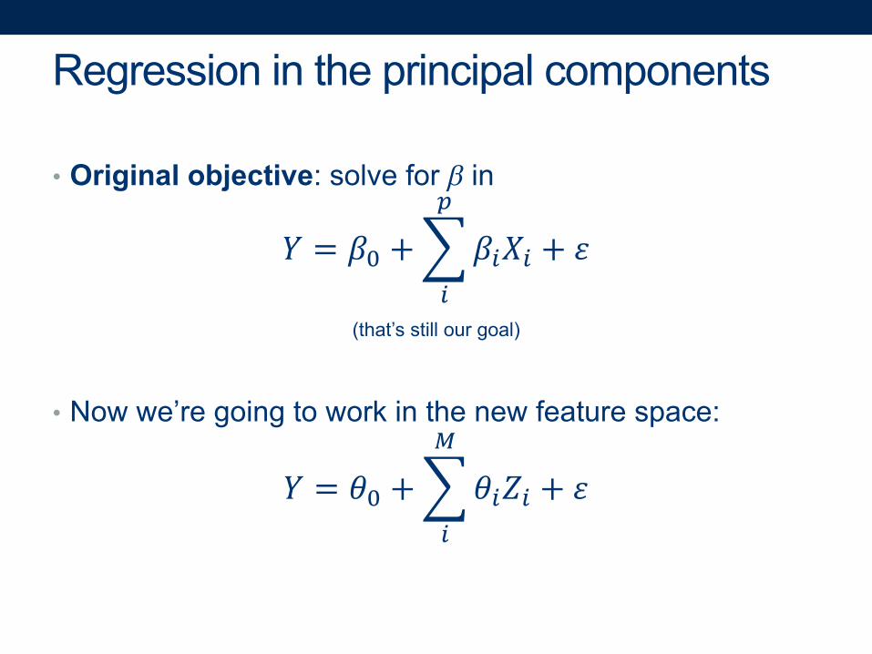
Regression in the principal components

• Original objective: solve for b in

. = 01 +304&4 + 7

5

4

(that’s still our goal)

• Now we’re going to work in the new feature space:

. = 81 +384-4 + 7

I

4

Regression in the principal components

• Remember: the new features are related to the old ones:

-: =3<4:&4

5

46'

• So we’re computing:

. = 81 +38:-: + 7

I

:6'

= 81 +38:3<4:&4

5

46'

+ 7

I

:6'

↦ 04 =38:<4:

I

:6'

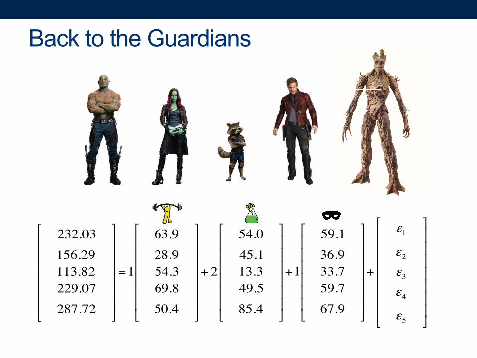
Back to the Guardians

232.03156.29113.82229.07287.72

⎡

⎣

⎢⎢⎢⎢⎢⎢

⎤

⎦

⎥⎥⎥⎥⎥⎥

=1

63.928.954.369.850.4

⎡

⎣

⎢⎢⎢⎢⎢⎢

⎤

⎦

⎥⎥⎥⎥⎥⎥

+ 2

54.045.113.349.585.4

⎡

⎣

⎢⎢⎢⎢⎢⎢

⎤

⎦

⎥⎥⎥⎥⎥⎥

+1

59.136.933.759.767.9

⎡

⎣

⎢⎢⎢⎢⎢⎢

⎤

⎦

⎥⎥⎥⎥⎥⎥

+

ε1

ε2ε3ε4

ε5

⎡

⎣

⎢⎢⎢⎢⎢⎢⎢

⎤

⎦

⎥⎥⎥⎥⎥⎥⎥

Back to the Guardians

• What happens if we use 2 components instead of 3?

Using only the principal components significantly improves our estimate!

i

i

-2

0

2

4

6 estimated - OLStrueestimated - PCR

Comparison with ridge regression and the lasso

• What similarities do you see?- Reduces dimensionality of the solution space (like Lasso)- Finds a solution in the space of all features (like RR)- Results can be difficult to interpret (like RR)

Problems with PCR

• We selected principal components based on predictors (not what we’re trying to predict!)

• This could be problematic (why?)-What if the values you’re trying to predict aren’t correlated with the

first few components?- You lose all predictive power!

Partial least squares (PLS)

• A supervised form of PCR• Feature derivation algorithm is similar:- Find the (M-1) principal most correlated components- Subtract the projection into that space- Maximize the variance correlation with the response in the

remaining complementary space

• As before, we perform least squares on the new features• We still use the formulation

-: =3<4:&4

5

46'

• But now f is computed by applying linear regression to eachpredictor

Wrapping up: PCR/PLS comparison

• Both derive a small number of orthogonal predictors for linear regression

• PCR is more biased- Emphasizes stability at the expense of versatility

• PLS estimates have higher variance-May build new features that aren’t as stable- But high variance is better than infinite variance

Lab: PCR and PLS

• To do today’s lab in R: pls

• To do today’s lab in python: <nothing new>

• Instructions and code:[course website]/labs/lab11-r.html

[course website]/labs/lab11-py.html

• Full version can be found beginning on p. 256 of ISLR

^E?H@6?3Q*'HDM78@7857H

,S?C7'387GA4*'-ABC'-?E?WQ@?S

!1!

"#

!

"#height = +!2

!

"#

!

"#+!3

!

"#

!

"#

!

"

!

"

"H4AS?4ABC'_D?8GA?BH\'`7AC@4

232.03156.29113.82229.07287.72

!

"

######

$

%

&&&&&&

=1

63.928.954.369.850.4

!

"

######

$

%

&&&&&&

+ 2

54.045.113.349.585.4

!

"

######

$

%

&&&&&&

+1

59.136.933.759.767.9

!

"

######

$

%

&&&&&&

+

!1

!2!3!4

!5

!

"

#######

$

%

&&&&&&&

"H4AS?47'P58'!

F [@7B'N7'48W'45'7H4AS?47'DHABC'0!/;'N7'C74'4@7'P5EE5NABC*

O&7E?4AI7EWR'@DC7'GAPP787B37'674N77B'?34D?E'?BG'7H4AS?47G'357PPA3A7B4H

"

"

12

3

2

4

5 $&-"#/-$*-)+$

! "#$ %%

F /5S7'GAS7BHA5BH'?87'87GDBG?B4- !A44E7'ABP58S?4A5B'AB')8G GAS7BHA5B'B54'3?M4D87G'6W'4@7'PA8H4'4N5- ,B'EAB7?8'87C87HHA5B;'87GDBG?B3W'3?DH7H'B5AH7'45'67'/#67"8"$*

232.03156.29113.82229.07287.72

!

"

######

$

%

&&&&&&

=1

63.928.954.369.850.4

!

"

######

$

%

&&&&&&

+ 2

54.045.113.349.585.4

!

"

######

$

%

&&&&&&

+1

59.136.933.759.767.9

!

"

######

$

%

&&&&&&

+

!1

!2!3!4

!5

!

"

#######

$

%

&&&&&&&

[@?4\H'C5ABC'5B'@787Z

a85b734A5B

a85b734A5B

!AB7?8'M85b734A5B

F .7N'P7?4D87H'?87'7"%$/)(,'#;"%/-"'%&(5P'58ACAB?E'G?4?*

-: / 384:&4

9

4F @AB2CC*'SDE4AMEWABC'4@7'*$"$+)$"#,- 6W'?'!#(./0",(%+)$"#,-

-' -( / &' &( &) &* &+

;'%';(%'

;'%(;(%(

;)%';*%';+%'

;)%(;*%(;+%(

[@?4\H'4@7'G7?E'NA4@'M85b734A5BZ

F +?4?'3?B'67'854?47G;'H3?E7G;'?BG'48?BHE?47G NA4@5D4'3@?BCABC'4@7'+%*$)7D"%?()$7/-"'%&="6&

F $@AH'S7?BH'W5D\87'?EE5N7G'45'E55Q'?4'4@7'G?4?'P85S'N@?47I78'?BCE7'S?Q7H'W5D8'EAP7'7?HA78c

%HABC'E5?GABCH'45'M85b734

-DE4AMEW'6W'E5?GABC'I73458'45'M85b734 OTHS55H@UR'7?3@'56H78I?4A5B'5B45'4@7'EAB7*

@4' / <''A4' 2 <('A4( 2 =2 <5'A45

$@7H7'I?ED7H'?87'3?EE7G'4@7'&,')$&5P'4@7'(H4 M8AB3AM?E'35SM5B7B4

&7C87HHA5B AB'4@7'M8AB3AM?E'35SM5B7B4H

F 3/)/)4/#*'4@7'B7N'P7?4D87H'?87')$7/-$*(45'4@7'5EG'5B7H*

-: / 3<4:&4

5

46'F /5'N7\87'35SMD4ABC*

. / 81 238:-: 2 7I

:6'

HHHHHHHHHHHHHHHHHH/ 81 238: 3<4:&4

5

46'2 7

I

:6'

, 04 / 38:<4:

I

:6'HHHHHHHHHHHHHHHHHHHHH

L?3Q'45'4@7'_D?8GA?BH

232.03156.29113.82229.07287.72

!

"

######

$

%

&&&&&&

=1

63.928.954.369.850.4

!

"

######

$

%

&&&&&&

+ 2

54.045.113.349.585.4

!

"

######

$

%

&&&&&&

+1

59.136.933.759.767.9

!

"

######

$

%

&&&&&&

+

!1

!2!3!4

!5

!

"

#######

$

%

&&&&&&&

L?3Q'45'4@7'_D?8GA?BH

F [@?4'@?MM7BH'AP'N7'DH7'9'35SM5B7B4H'ABH47?G'5P')Z

%HABC'5BEW'4@7'M8AB3AM?E'35SM5B7B4H'HACBAPA3?B4EW'ASM85I7H'5D8'7H4AS?47g

"

"

12

3

2

4

5 $&-"#/-$*(1 FH:-)+$$&-"#/-$*(1 I9J

#5SM?8AH5B'NA4@'8AGC7'87C87HHA5B'?BG'4@7'E?HH5

F [@?4'HASAE?8A4A7H'G5'W5D'H77Z- &7GD37H'GAS7BHA5B?EA4W'5P'4@7'H5ED4A5B'HM?37'OEAQ7'!?HH5R- ^ABGH'?'H5ED4A5B'AB'4@7'HM?37'5P'?EE'P7?4D87H'OEAQ7'&&R- &7HDE4H'3?B'67'GAPPA3DE4'45'AB478M874'OEAQ7'&&R

a856E7SH'NA4@'a#&

F [7'H7E7347G'M8AB3AM?E'35SM5B7B4H'6?H7G'5B'M87GA3458H'OB54'N@?4'N7\87'48WABC'45'M87GA34gR

F $@AH'35DEG'67'M856E7S?4A3'ON@WZR-[@?4'AP'4@7'I?ED7H'W5D\87'48WABC'45'M87GA34'?87B\4'35887E?47G'NA4@'4@7'

PA8H4'P7N'35SM5B7B4HZ- 25D'E5H7'?EE'M87GA34AI7'M5N78g