lecture 12: lidarand aerial image

Lecture 12: LiDAR and aerial image

Yuji Kuwano, Lead ALS Support Engineer

Leica Geosystems AG

Please insert a picture

(Insert, Picture, from file).

Size according to grey field

(10 cm x 25.4 cm).

Scale picture: highlight, pull corner point

Cut picture: highlight, choose the cutting icon from the picture tool bar, click on a

side point and cut

2

Presentation outline

Introduction to digital frame camera workflow

Demonstration of camera boresight workflow

Demonstration of orthophoto workflow with case study

Summary

3

RCD105 Digital Frame Camera for ALS50-II

39 MP: flexible and fast

Certified airborne design

High shutter speed (1/4000 sec), high frame rate (2.02 seconds/frame)

3 lenses to choose from (35, 60, 100 mm) with RGB or CIR

Up to 2 camera heads per controller

4

RCD105 Camera System

product configuration

CH39 Camera Head (39 MP)

Lens (35, 60 or 100 mm)

CC105 Camera Controller (shown

mounted to SC50System Controller)

Isolated Interface Plate Assembly (Mi-8

version shown)

5

RCD105 integration with ALS50-II

(green indicates RCD105 components)

AUX1 Hybrid

AUX1 LAN

SC50

Hybrid

LAN

CC105 Camera

Controller

SDR-26

CH39 Camera Head

Lens

(35, 60

or 100

mm)

RGB FilterShutte

r

Optional CIR

Filter and

Compensating

Optic

�28 VDC

Mid-exposure pulse (TTL) ��

�Real-time nav solution (GPS time,

position, orientation)

Trigger, pixel

data, serial

camera control

or

12 VDC, mid-

exposure

pulse

Lemo

SDR-26 Lemo

6

Camera workflow overview

in context of LIDAR workflow

FPES

Mission

Planningmode

altitude

scan rate

FOV

flight speed

flight lines

flight height

lens FL

shutter speed

frame rate

record DGPS base

station data

Airborne

Operationsrecord position and attitude data

•GPS

•IMU

•event marks

record scanner data

•range

•scan angle

•intensity

•timing info

record camera data

•photo ID file

•raw frames

extract

position

and

attitude

data

DGPS

processing

trajectory

processing

•point cloud generation

•output formatting – LDI, LAS, ASCII

•projection - WGS 84, UTM, state plane, Swiss, TW 97, user-supplied

•datum (state plane only) - NGVD 29, NAVD 88

•tiling

•coverage verification

•outlier removal

•bare earth

•thinning

•catenary generation

deliverables

Ground

Operations

Planning Collection Processing

real-time nav file

*.SCN raw scanner files

ALS50, FCMS, CamGUI

GrafNav IPAS Pro

ALS50 Post Processor

position and

attitude file

GPS1200

TerraScan

IPAS Pro

Micro

Statio

n

•TIN/contour

•control report

TerraModeller

laser boresite

calibration

Attune

calculate

exterior

orientations

EO fileIPAS CO

camera

boresight,

orthophoto

generation

LPS

“LAS” file

orthophotos

Bayer

conversion

CDPP

7

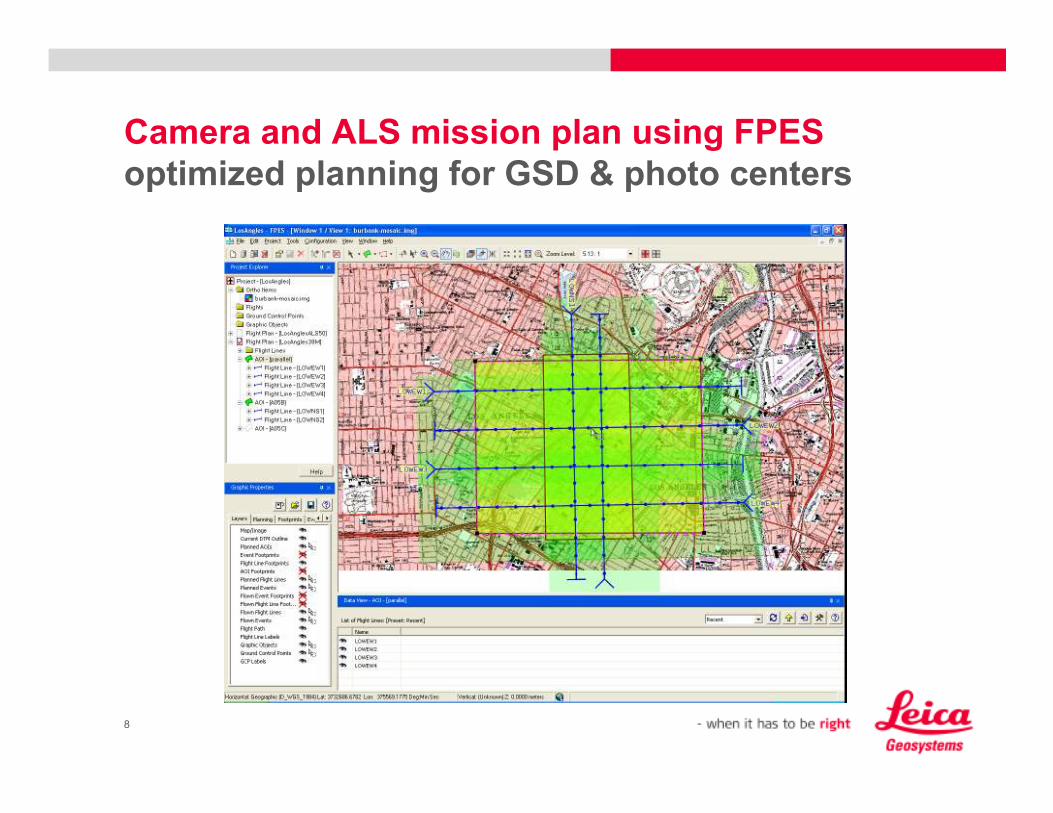
Mission planning objectives

coordinating sensor and aircraft parameters

Determine camera settings

� Determine ground sample distance

� Select lens and flying height

� Determine coverage

� Select forward overlap

� Determine shutter speed

Determine flight line layout

� Line-to-line spacing

� Photo centers

8

Camera and ALS mission plan using FPES

optimized planning for GSD & photo centers

9

Camera boresight flight plan

2 flight levels and directions required for boresight

Can perform without ground control

Recommended calibration configuration (60 mm lens example)

� Mission area

� Roughly 3km x 2.5km

� Overlap / sidelap

� 60% forward, 40% sidelap

� 15 cm GSD @ 1350 m AGL

� 4 Parallel lines / opposed flight direction

� 12 Images per lines

� 25 cm GSD @ 2300 m AGL

� 2 cross lines / opposed flight direction

� 6 Images per lines

� Ground Control Point (Recommended)

� Locate 4 corners and center,3 alternatives for each area

� Accuracy check as check point

Ground Control Point

10

Camera vs. altitude parameters

achieving correct pixel size and area coverage

3670

2300

1280

Altitude

AGL

(m)

2200

1350

770

Altitude

AGL

(m)

Higher Altitude

Along track x

Cross track

for 15cm lines

(km x km)

GSD

(m)

GSD

(m)

3.5 x 2.80.250.15100

3.0 x 2.50.250.1560

3.5 x 3.00.250.1535

Estimated

Calibration

Area

Coverage

Lower Altitude

Focal

Length

(mm)

11

Camera boresight

IPAS CO Setup

12

Camera boresight

IPAS CO Initial EO ‘Seeded.dat’

File structure : EventID , ImageID , X , Y , Z , O , P , K

13

Set up LPS project

define coordinate system, projection and datum

14

Set up LPS project

create a camera file ( Use Balanced parameter )

� Use supplied K01,K1,K2 coefficient

15

Set up LPS project

import Initial EO information

16

Set up LPS project

initial mage location

17

LSP project

check initial misalignment quality using ViewPlex

18

LPS project

automatic tie point measurement

19

LPS project

triangulation properties – “General” tab

20

LPS project

triangulation properties – “Point” tab

21

LPS project

triangulation properties – “Exterior” tab

22

LPS project

triangulation properties – “Advanced Options” tab

23

LPS project

triangulation summary

24

LPS project

manual blunder rejection (as needed)

25

LPS project

triangulation report

26

LPS project

updated exterior orientation

27

Camera boresight

IPAS CO “Compute Camera Misalignment” setup

28

Camera boresight

IPAS CO “Camera Misalignment Results” window

29

Direct georeferencing

IPAS CO setup

30

Direct referencing

IPAS CO final EO

31

LSP project

check final misalignment quality using ViewPlex

32

Case Study 1…higher productivity with MPiA

42.5 HzScan rate

45 degreesFOV

150 kHz

(MPiA)Pulse rate

LIDAR

parameters

100 knotsAircraft speed

Aircraft

parameters

Cross-track

post spacing

(worst case)

Along-track

post spacing

(worst case)

Flying height

0.91 m

1.21 m

1300 m AGL

Palos Verdes

33

Case Study 1…higher productivity with MPiA

42.5 HzScan rate

45 degreesFOV

150kHz

(MPiA)Pulse rate

LIDAR

parameters


Aircraft

parameters

Cross-track

post spacing

(worst case)

Along-track

post spacing

(worst case)

Flying height

1.21 m

0.91 m

1300 m AGL

42.5 HzScan rate

45 degreesFOV

104kHz

(SPiA)Pulse rate

LIDAR

parameters


Aircraft

parameters

Cross-track

post spacing

(worst case)

Along-track

post spacing

(worst case)

Flying height

1.21 m

0.92 m

910 m AGL

ALS50/SPiA ModeALS50/MPiA Mode

34

Case Study 1…bare earth surface generation

sample small section

1 flight line

1.0km x 1.6 km covered

Total of 2 523 721 points

Multiple returns

Image features all LIDAR points

colored by elevation

35

Case Study 1…filtering of laser surface

ground surface model (DTM) is now created

Step 1. Classify “Ground’ Model for bare earth classification

(1 385 128 points to the ground)

36

Case Study 1…filtering of laser surface…cont


Step 2. Thin ground surface using “model key points” routine

Ground surface is now defined by 139 756 points

37

Case Study 1…form photogrammetric block

Sample 1 strip of 4 images

Each strip has with 60% forward overlap

Nominal GSD size 15cm

Camera fixed to LIDAR scanner platform; therefore no drift

compensation available for the camera

Format size 7162 (cross track) x 5389 (along track)

38

Case Study 1…direct georeferencing

IPAS CO using same misalignment from calibration

39

Case Study 1…ortho production

setup LPS project / import direct georeference data

40


exterior orientation is fixed

41


check stereo pair quality (paralax) using ViewPlex

42

Case Study 1…importing the LIDAR DTM

direct LAS file import facilitates orthorectification

A terrain model is required to generate orthophotos

The model key point surface can be imported directly in LIDAR

native LAS file format

A gridded DTM is generated at 2m interval (i.e., greater than the

LIDAR post spacing)

43

Case Study 1…LPS surface import setup

44

Case Study 1…view of output gridded DTM

45

Case Study 1…LPS orthophoto resampling setup

46

Case Study 1…0.15 m orthophoto generation with ALS50

includes surface, EO information, camera model, images

47

Case Study 1…0.15 m orthophoto generation with ALS50

individual ortho has good match with ALS DTM

48

Case Study 1…LPS ortho mosaic setup

49

Case Study 1…LPS ortho mosaic

(before color dodging)

50

RCD105 Digital Frame Camera for ALS50-II

rugged design for precise imagery

51

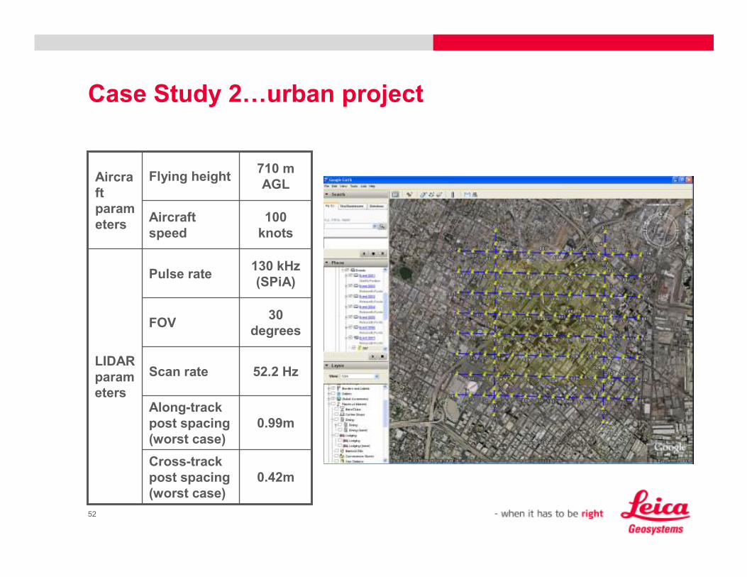
Case Study 2…urban project

ortho with bare earth DTM vs dense LIDAR DSM

0.42 mCross-track post spacing (worst case)

52.2 HzScan rate

30 degreesFOV

124kHz (SPiA)Pulse rate

LIDAR parameters


Aircraft parameters

Average Point Density (@ Nadir)

Along-track post spacing (worst case)

Flying height

4.31 pts/m^2

0.99 m

710 m AGL

52

Case Study 2…urban project

52.2 HzScan rate

30

degreesFOV

130 kHz

(SPiA)Pulse rate

LIDAR

param

eters

100

knots

Aircraft

speed

Aircra

ft

param

eters

Cross-track

post spacing

(worst case)

Along-track

post spacing

(worst case)

Flying height

0.42m

0.99m

710 m

AGL

Palos Verdes

53

Case Study 2…LIDAR surface generation (bare earth / DSM)

small sample area

2 flight lines

0.8km x 0.6 km covered

Total of 3 774 070 points

Multiple returns

Image features all LIDAR

points colored by elevation

54

Case Study 2…bare earth extraction


Step 1. Classify “Ground’ Model for bare earth classification

(978 030 points to the ground)

Step2.Classify ‘Model Key Point’ to LAS file(47 972 points)

55

Case Study 2…DSM extraction

Step 1. Classify ‘Any First return’ points(3 708 569 points)

Step 2. Export Any of First to LAS file as DSM

56

Case Study 2…form photogrammetric block

Sample 1 strip of 4 images

Each strip has with 60% forward overlap

Nominal GSD size 8 cm

Camera fixed to LIDAR scanner platform; therefore no drift

compensation available for the camera

57

Case Study 2…direct georeferencing

IPAS CO setup…same misalignment from calibration

58


exterior orientation is fixed

59


check stereo pair quality by ViewPlex

60

Case Study 2…importing the LIDAR DTM

direct LAS file import facilitates orthorectification

Create 2 sets of DTM for comparison

A) Bare Earth DTM as conventional Ortho workflow

-Import by 2m Gridded DEM

B) DSM as True Ortho aiding

-Import by original point spacing(=0.45m point spacing) DEM

61

Case Study 2…view of gridded bare earth DTM

62

Case Study 2…view of gridded DSM

63

Case Study 2…LPS orthophoto resampling setup

64

Case Study 2…8 cm GSD orthophoto with bare earth

individual ortho images

65

Case Study 2…8 cm GSD orthophoto with bare

earth

Bare earth DTM provides very good

ortho matching

Note building lean in images due to

off-nadir angle

66

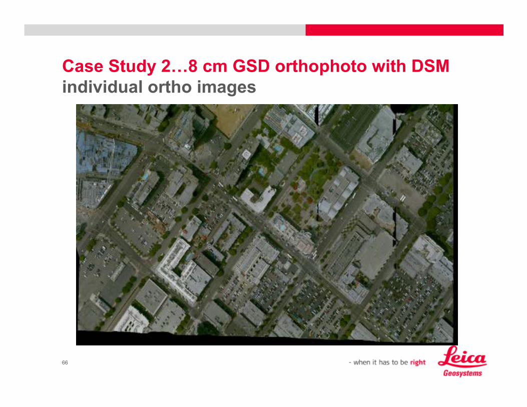
Case Study 2…8 cm GSD orthophoto with DSM

individual ortho images

67

Case Study 2…8 cm GSD orthophoto with DSM

DSM ortho minimizes number of buildings needing

vectorization

68

Case Study 2…bare earth ortho vs DSM ortho

Bare Earth Ortho Dense DSM Ortho

69

Conclusions

IPAS CO and LPS Core/ORIMA can be used to determine camera

boresight and compute direct exterior orientation for images

Orthophoto workflow is well integrated with LIDAR workflow

LPS software is well-suited to the task of handling LIDAR data for

orthorectification

High density ALS data aids generation of true ortho product

70

Thank you

questions?

[email protected]

Leica Geosystems AG

Heinrich-Wild-Strasse

CH-9435 Heerbrugg ,Switzerland

Tell+41 71 727 4262

Fax+41 71 727 4674

lecture 12: lidarand aerial image

Documents