lecture 09 morphological image processing
TRANSCRIPT

LECTURE 09MORPHOLOGICAL
IMAGE PROCESSING
2110431 INTRODUCTION TO DIGITAL IMAGING2147329 DIGITAL IMAGE PROCESSING AND VISION SYSTEMS
Punnarai Siricharoen, Ph.D.
OBJECTIVES
• To understand basic morphological image processing techniques
• To be able to apply morphological techniques as development basis for segmentation, automated inspection, or describing an image with the simple to moderate complexity of the problems
2
CONTENT
• Introduction
• Logic operation with binary images
• Dilation / Erosion
• Closing / Opening
• Hit-or-miss transformation
• Other morphological algorithms
• Thinning/Thickening/Skeleton/Pruning
• Applications of grayscale morphology
3
INTRODUCTION
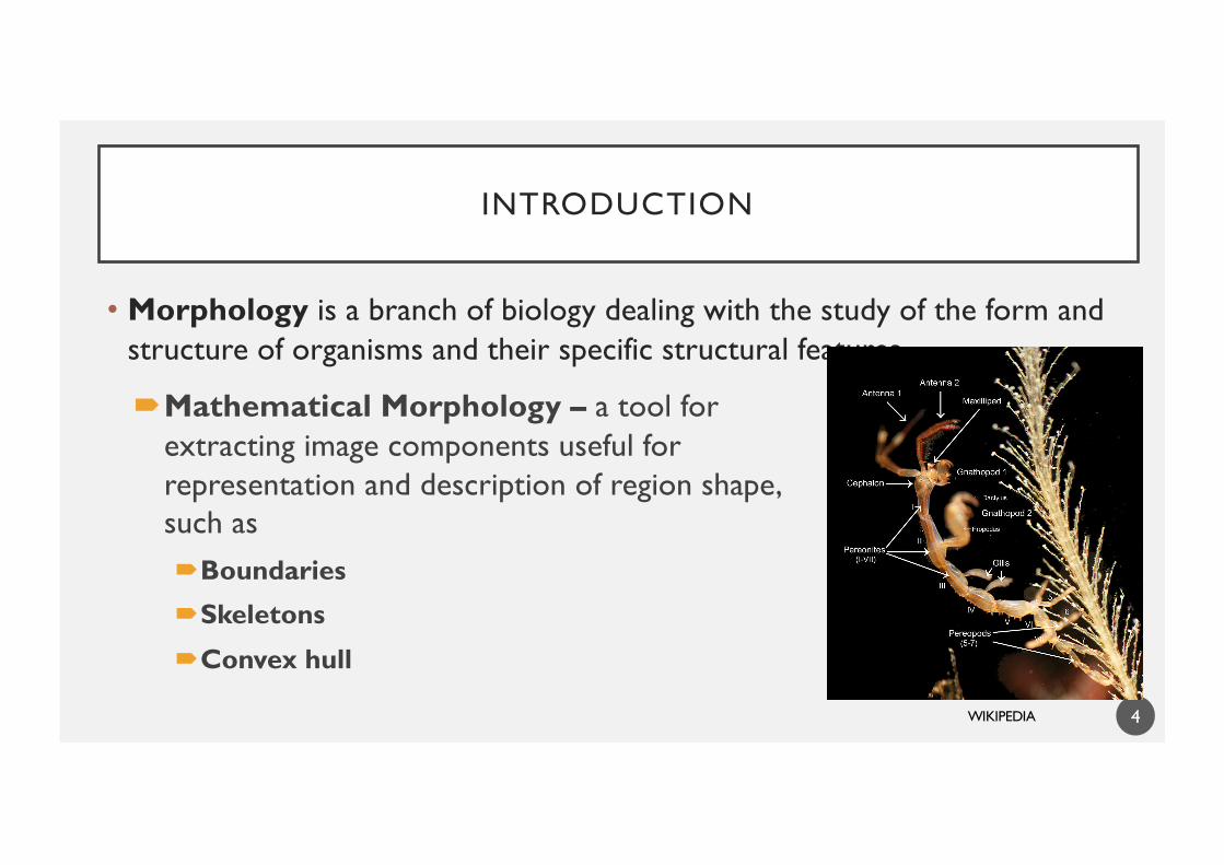
• Morphology is a branch of biology dealing with the study of the form and structure of organisms and their specific structural features.
4
´Mathematical Morphology – a tool for extracting image components useful for representation and description of region shape, such as´Boundaries
´Skeletons
´Convex hull
WIKIPEDIA
INTRODUCTION
• Morphological techniques – pre or post-processing, such as morphological filtering, thinning and pruning.
5
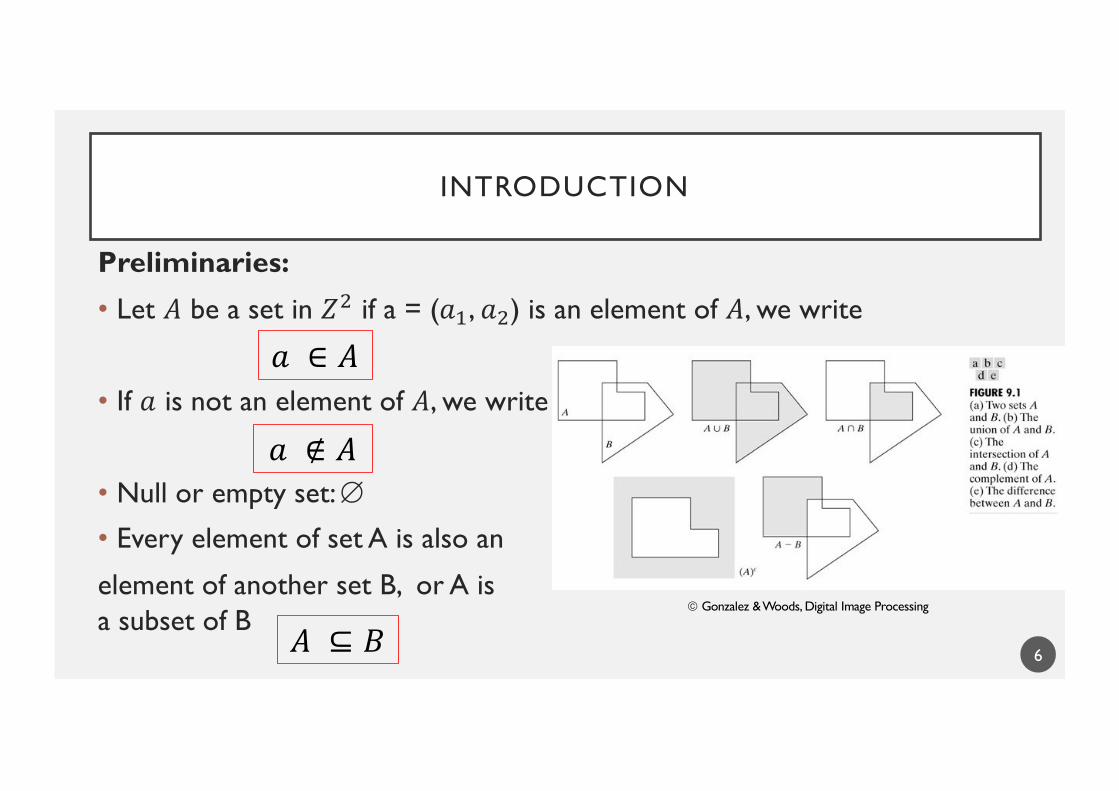
INTRODUCTION
Preliminaries:
• Let 𝐴 be a set in 𝑍! if a = (𝑎", 𝑎!) is an element of 𝐴, we write
• If 𝑎 is not an element of 𝐴, we write
• Null or empty set: Æ
• Every element of set A is also an
element of another set B, or A is a subset of B
6
𝑎 ∈ 𝐴
𝑎 ∉ 𝐴
ã Gonzalez & Woods, Digital Image Processing
𝐴 ⊆ 𝐵
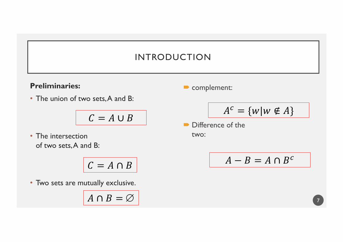
INTRODUCTION
Preliminaries:
• The union of two sets, A and B:
• The intersectionof two sets, A and B:
• Two sets are mutually exclusive.
7
𝐶 = 𝐴 ∪ 𝐵
𝐶 = 𝐴 ∩ 𝐵
𝐴 ∩ 𝐵 = Æ
´ complement:
´ Difference of thetwo:
𝐴! = {𝑤|𝑤 ∉ 𝐴}
𝐴 − 𝐵 = 𝐴 ∩ 𝐵!
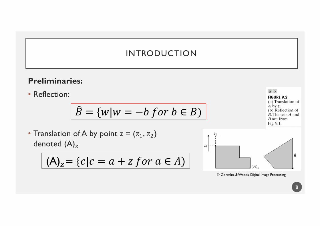
INTRODUCTION
Preliminaries:
• Reflection:
• Translation of A by point z = (𝑧", 𝑧!) denoted (A)#
8
!𝐵 = {𝑤|𝑤 = −𝑏 𝑓𝑜𝑟 𝑏 ∈ 𝐵)
(A)!= {𝑐|𝑐 = 𝑎 + 𝑧 𝑓𝑜𝑟 𝑎 ∈ 𝐴)ã Gonzalez & Woods, Digital Image Processing
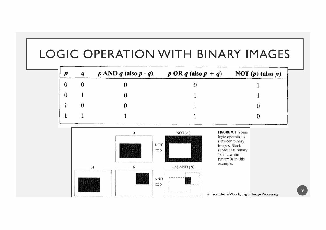
LOGIC OPERATION WITH BINARY IMAGES
9ã Gonzalez & Woods, Digital Image Processing
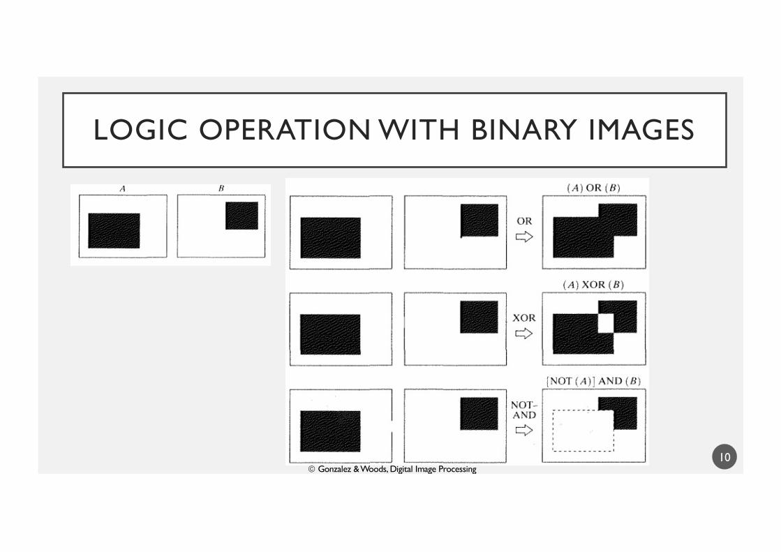
LOGIC OPERATION WITH BINARY IMAGES
10ã Gonzalez & Woods, Digital Image Processing
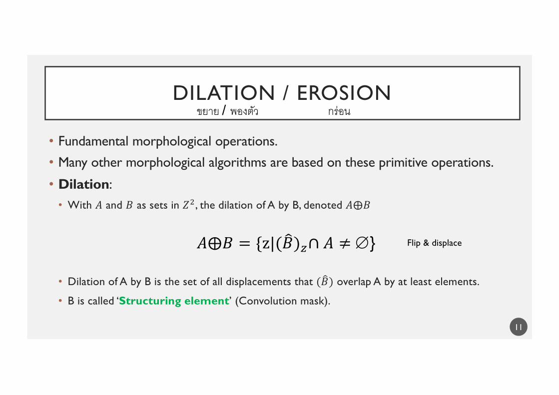
DILATION / EROSION
• Fundamental morphological operations.
• Many other morphological algorithms are based on these primitive operations.
• Dilation:• With 𝐴 and 𝐵 as sets in 𝑍!, the dilation of A by B, denoted 𝐴⨁𝐵
• Dilation of A by B is the set of all displacements that ( &𝐵) overlap A by at least elements.
• B is called ‘Structuring element’ (Convolution mask).
11
ขยาย / พองตวั กร่อน
𝐴⨁𝐵 = {z|( 3𝐵)"∩ 𝐴 ≠ Æ} Flip & displace
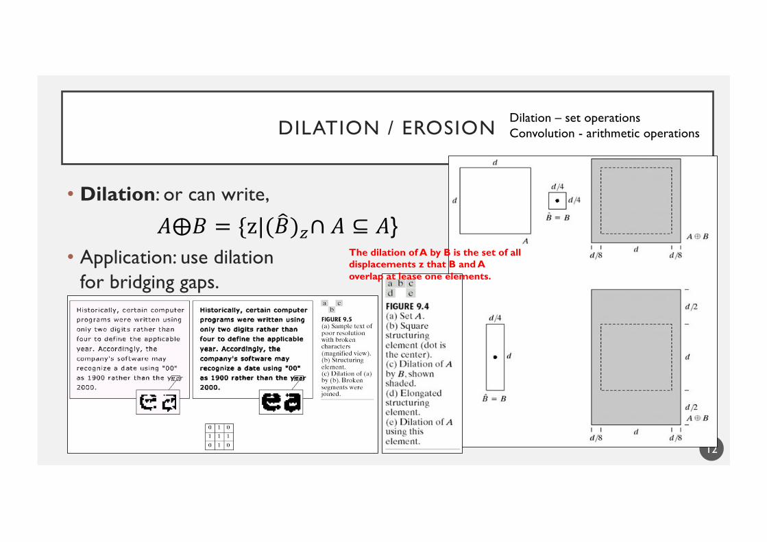
DILATION / EROSION
• Dilation: or can write,
• Application: use dilationfor bridging gaps.
12
Dilation – set operationsConvolution - arithmetic operations
𝐴⨁𝐵 = {z|( 3𝐵)"∩ 𝐴 ⊆ 𝐴}The dilation of A by B is the set of all displacements z that B and A overlap at lease one elements.
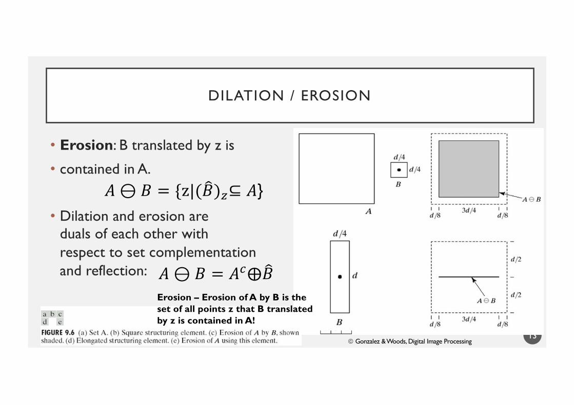
DILATION / EROSION
• Erosion: B translated by z is
• contained in A.
• Dilation and erosion are duals of each other withrespect to set complementationand reflection:
13
𝐴⊖ 𝐵 = {z|( 3𝐵)"⊆ 𝐴}
𝐴⊖ 𝐵 = 𝐴!⨁ 3𝐵Erosion – Erosion of A by B is the set of all points z that B translated by z is contained in A!
ã Gonzalez & Woods, Digital Image Processing
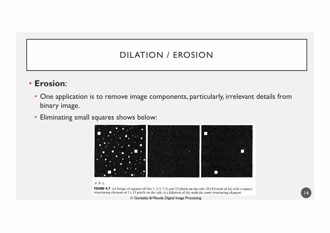
DILATION / EROSION
• Erosion:• One application is to remove image components, particularly, irrelevant details from
binary image.
• Eliminating small squares shows below:
14ã Gonzalez & Woods, Digital Image Processing
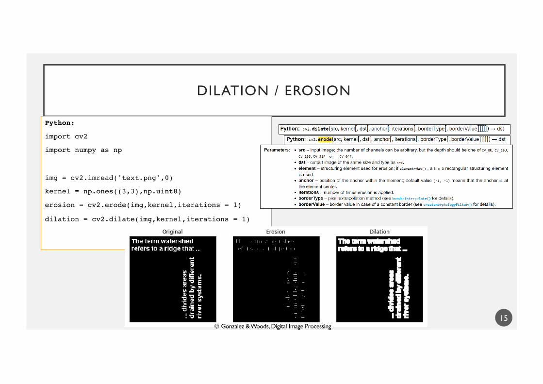
DILATION / EROSION
Python:
import cv2
import numpy as np
img = cv2.imread('text.png',0)
kernel = np.ones((3,3),np.uint8)
erosion = cv2.erode(img,kernel,iterations = 1)
dilation = cv2.dilate(img,kernel,iterations = 1)
15ã Gonzalez & Woods, Digital Image Processing
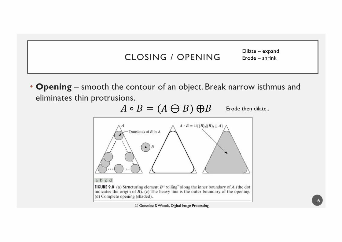
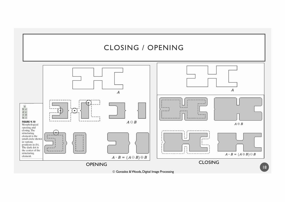
CLOSING / OPENING
• Opening – smooth the contour of an object. Break narrow isthmus and eliminates thin protrusions.
16
Dilate – expandErode – shrink
𝐴 ∘ 𝐵 = (𝐴 ⊖ 𝐵) ⨁𝐵 Erode then dilate..
ã Gonzalez & Woods, Digital Image Processing
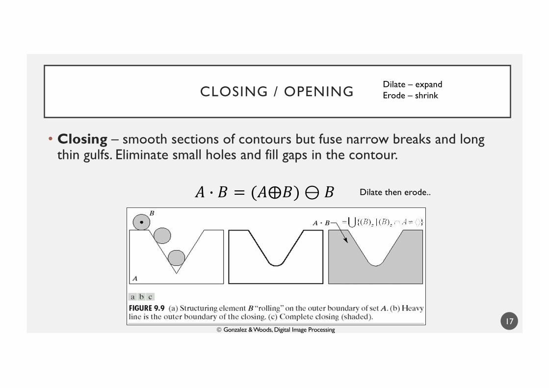
CLOSING / OPENING
• Closing – smooth sections of contours but fuse narrow breaks and long thin gulfs. Eliminate small holes and fill gaps in the contour.
17
Dilate – expandErode – shrink
𝐴 8 𝐵 = (𝐴⨁𝐵)⊖ 𝐵 Dilate then erode..
ã Gonzalez & Woods, Digital Image Processing
CLOSING / OPENING
18ã Gonzalez & Woods, Digital Image Processing
CLOSINGOPENING
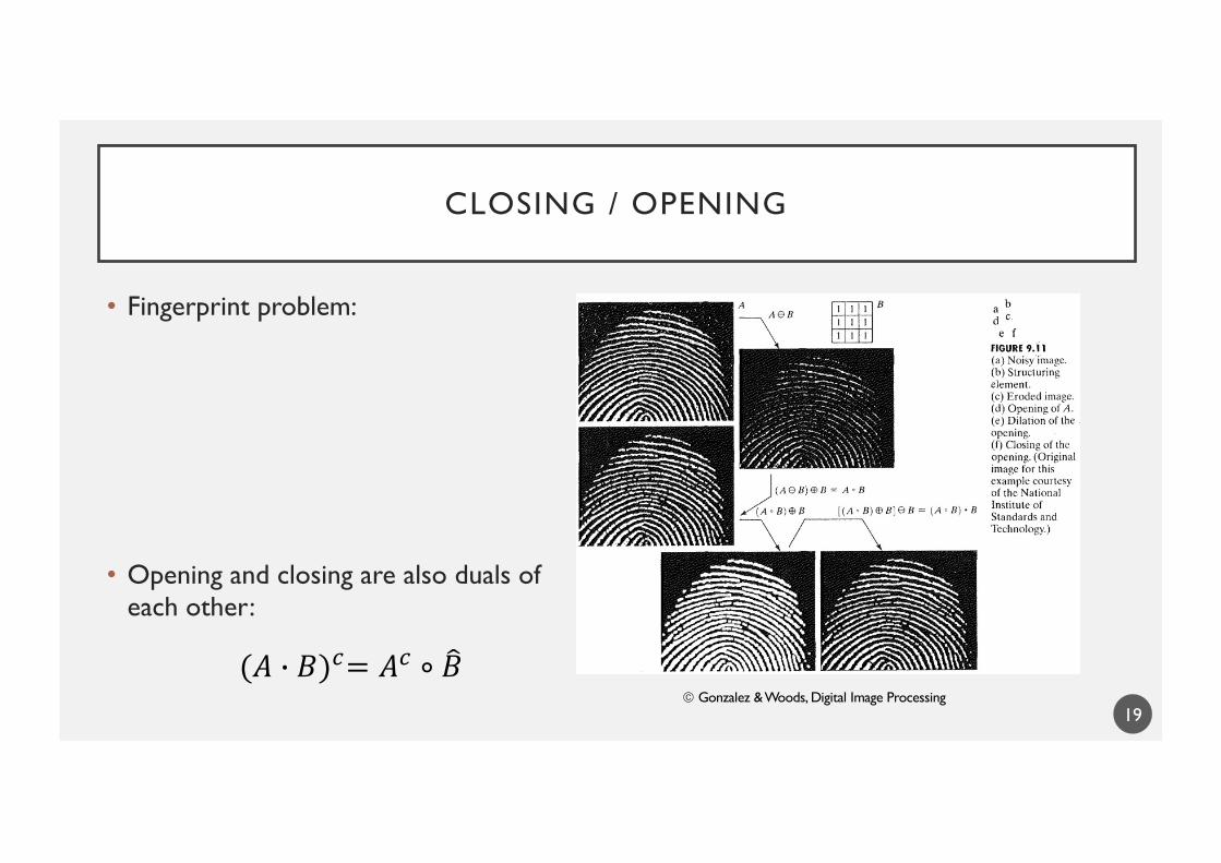
CLOSING / OPENING
• Fingerprint problem:
• Opening and closing are also duals of each other:
19
(𝐴 & 𝐵)$= 𝐴$ ∘ +𝐵ã Gonzalez & Woods, Digital Image Processing
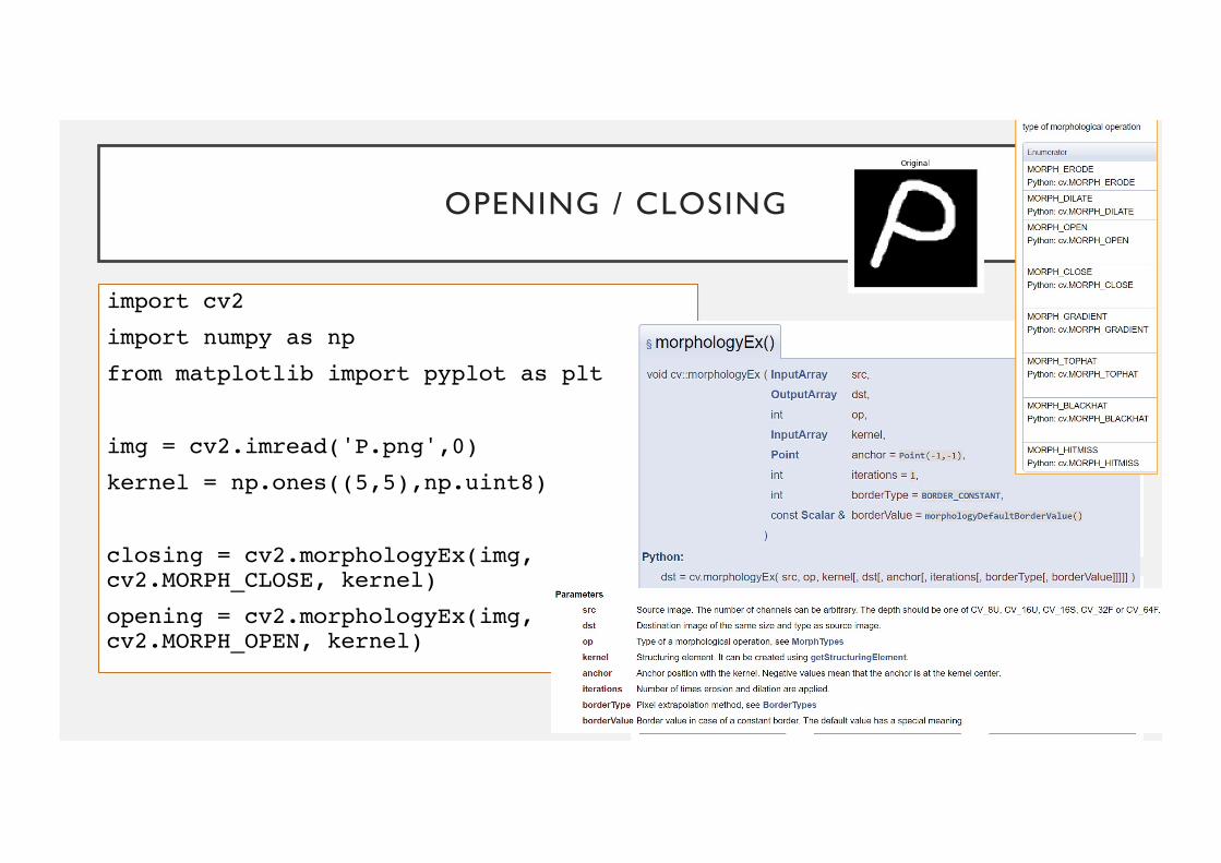
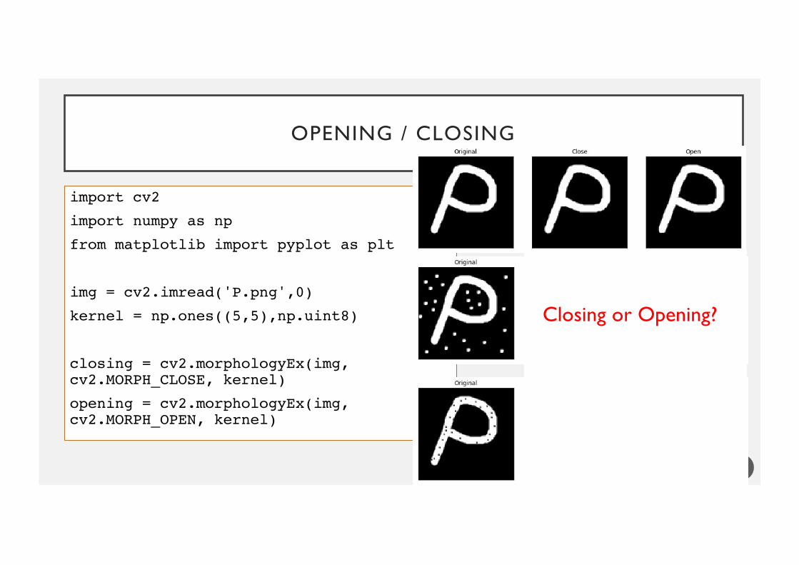
OPENING / CLOSING
import cv2
import numpy as np
from matplotlib import pyplot as plt
img = cv2.imread('P.png',0)
kernel = np.ones((5,5),np.uint8)
closing = cv2.morphologyEx(img, cv2.MORPH_CLOSE, kernel)
opening = cv2.morphologyEx(img, cv2.MORPH_OPEN, kernel)
20
import cv2
import numpy as np
from matplotlib import pyplot as plt
img = cv2.imread('P.png',0)
kernel = np.ones((5,5),np.uint8)
closing = cv2.morphologyEx(img, cv2.MORPH_CLOSE, kernel)
opening = cv2.morphologyEx(img, cv2.MORPH_OPEN, kernel)
OPENING / CLOSING
21
Closing or Opening?
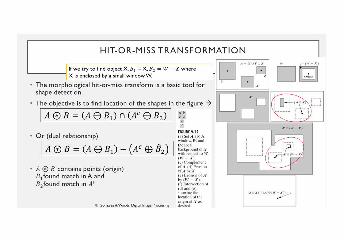
HIT-OR-MISS TRANSFORMATION
• The morphological hit-or-miss transform is a basic tool for shape detection.
• The objective is to find location of the shapes in the figure à
• Or (dual relationship)
• 𝐴 ⊛ 𝐵 contains points (origin) 𝐵"found match in A and 𝐵!found match in 𝐴#
22
𝐴⊛ 𝐵 = 𝐴⊖ 𝐵" ∩ 𝐴$ ⊖𝐵!
𝐴⊛ 𝐵 = 𝐴⊖ 𝐵" − 𝐴$ ⊕ +𝐵!
If we try to find object X, 𝐵! = X, 𝐵" = 𝑊 − 𝑋 where X is enclosed by a small window W.
ã Gonzalez & Woods, Digital Image Processing
SOME BASIC MORPHOLOGICAL ALGORITHMS
• Boundary extraction
• Region filling
• Extraction of connected components
• Convex Hull
• Thinning
• Skeletons
• Pruning
• Summary of Morphological Operations on binary images
23
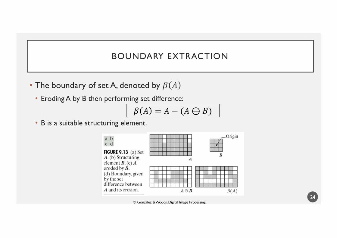
BOUNDARY EXTRACTION
• The boundary of set A, denoted by 𝛽 𝐴• Eroding A by B then performing set difference:
• B is a suitable structuring element.
24
𝛽 𝐴 = 𝐴 − (𝐴 ⊖ 𝐵)
ã Gonzalez & Woods, Digital Image Processing
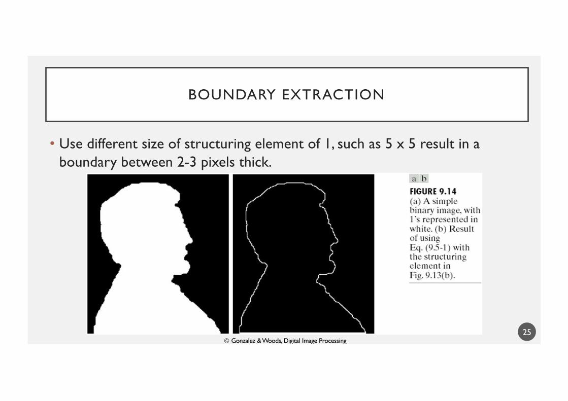
BOUNDARY EXTRACTION
• Use different size of structuring element of 1, such as 5 x 5 result in a boundary between 2-3 pixels thick.
25ã Gonzalez & Woods, Digital Image Processing
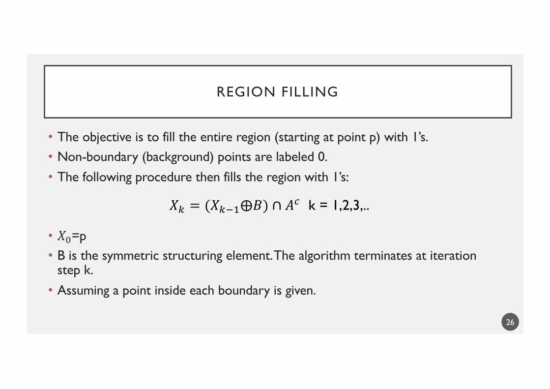
REGION FILLING
• The objective is to fill the entire region (starting at point p) with 1’s.• Non-boundary (background) points are labeled 0.• The following procedure then fills the region with 1’s:
• 𝑋!=p• B is the symmetric structuring element. The algorithm terminates at iteration
step k. • Assuming a point inside each boundary is given.
26
𝑋% = (𝑋%&"⨁𝐵) ∩ 𝐴$ k = 1,2,3,..
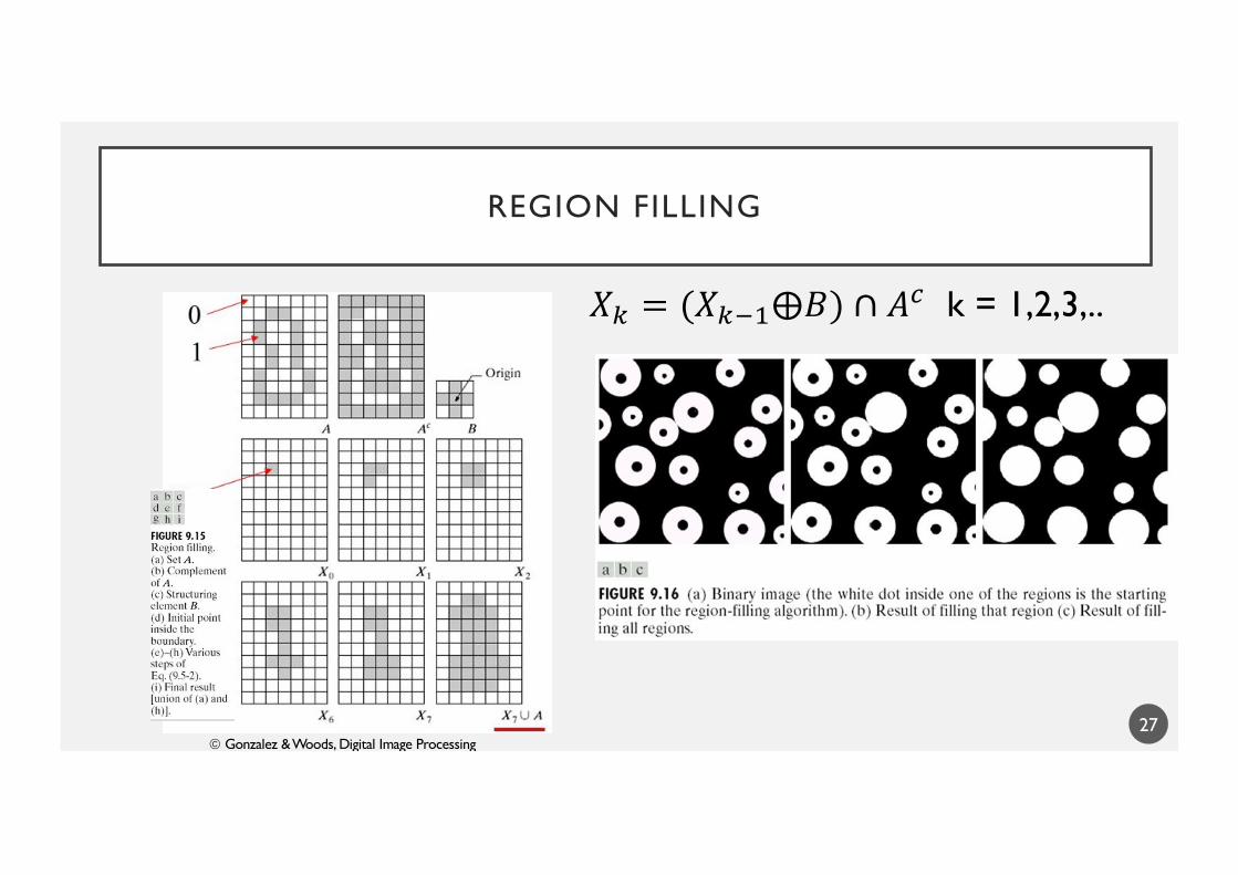
REGION FILLING
27
𝑋# = (𝑋#$%⨁𝐵) ∩ 𝐴! k = 1,2,3,..
ã Gonzalez & Woods, Digital Image Processing
EXTRACTION OF CONNECTED COMPONENTS
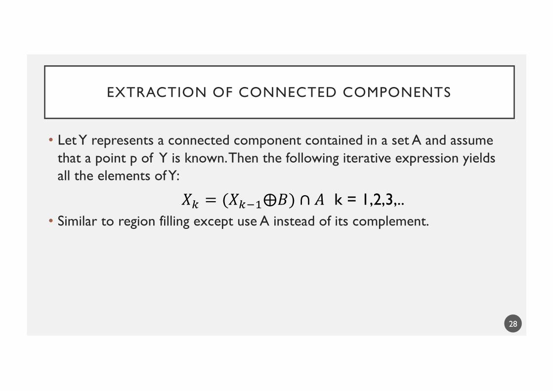
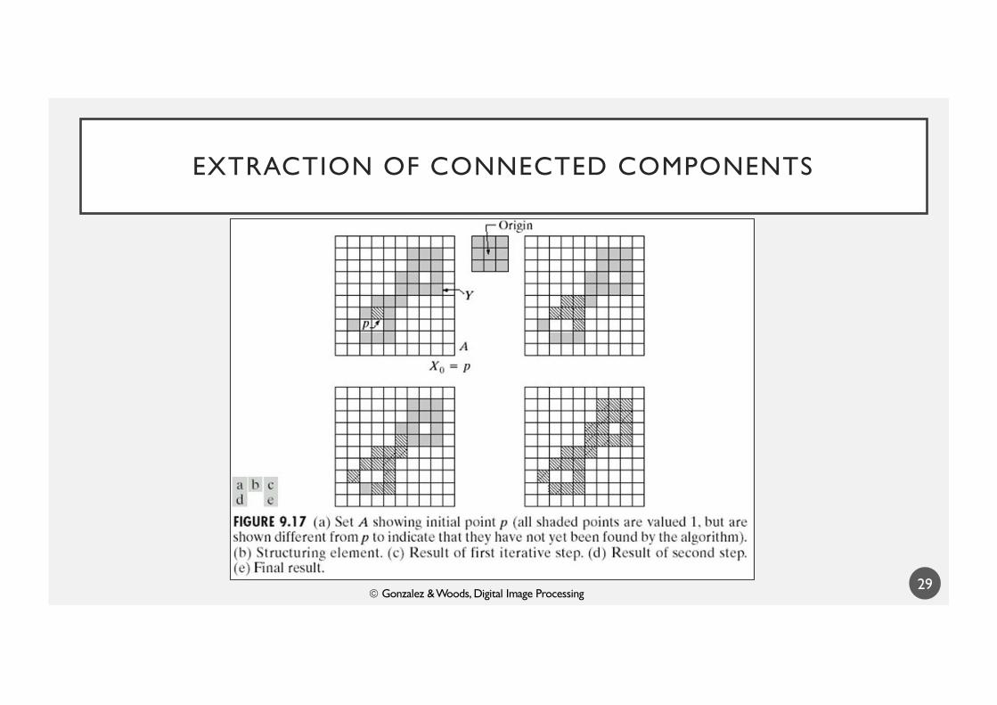
• Let Y represents a connected component contained in a set A and assume that a point p of Y is known. Then the following iterative expression yields all the elements of Y:
• Similar to region filling except use A instead of its complement.
28
𝑋# = (𝑋#$%⨁𝐵) ∩ 𝐴 k = 1,2,3,..
EXTRACTION OF CONNECTED COMPONENTS
29ã Gonzalez & Woods, Digital Image Processing
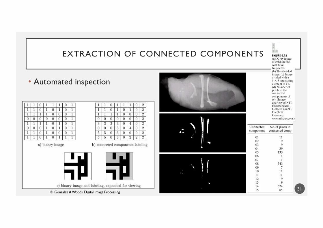
EXTRACTION OF CONNECTED COMPONENTS
• Automated inspection
31ã Gonzalez & Woods, Digital Image Processing
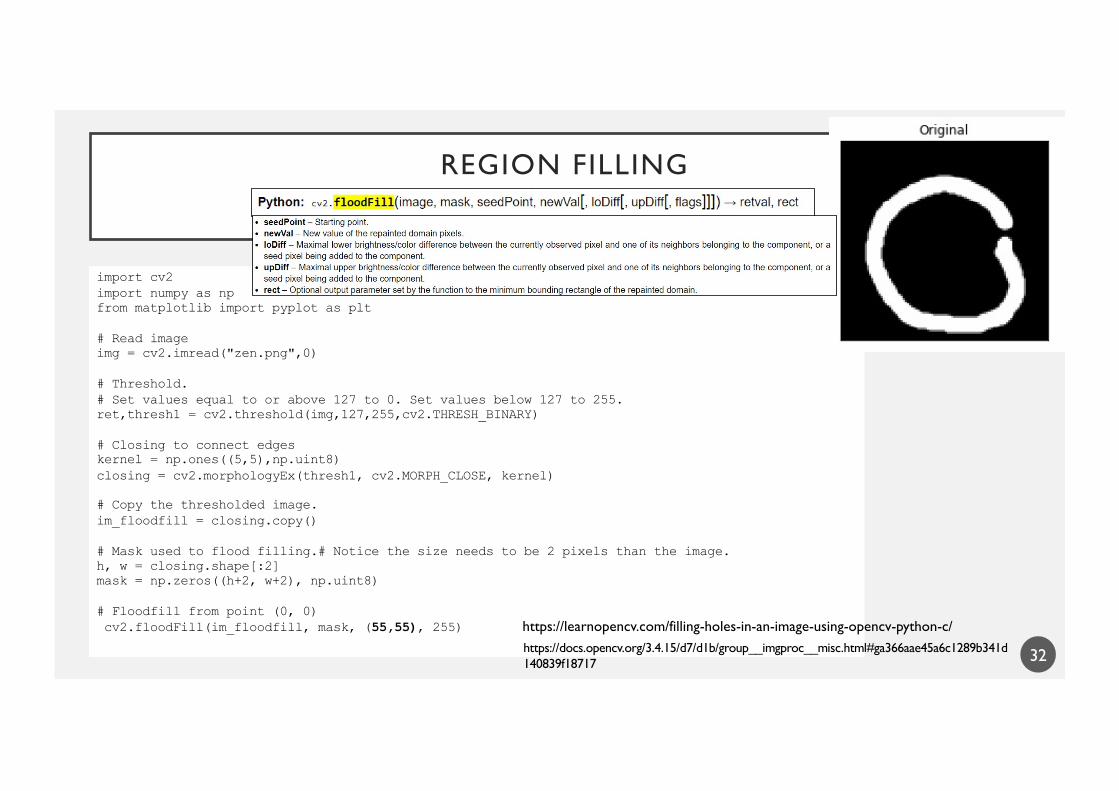
REGION FILLING
32
import cv2import numpy as npfrom matplotlib import pyplot as plt
# Read imageimg = cv2.imread("zen.png",0)
# Threshold.# Set values equal to or above 127 to 0. Set values below 127 to 255. ret,thresh1 = cv2.threshold(img,127,255,cv2.THRESH_BINARY)
# Closing to connect edgeskernel = np.ones((5,5),np.uint8)closing = cv2.morphologyEx(thresh1, cv2.MORPH_CLOSE, kernel)
# Copy the thresholded image.im_floodfill = closing.copy()
# Mask used to flood filling.# Notice the size needs to be 2 pixels than the image.h, w = closing.shape[:2]mask = np.zeros((h+2, w+2), np.uint8)
# Floodfill from point (0, 0)cv2.floodFill(im_floodfill, mask, (55,55), 255) https://learnopencv.com/filling-holes-in-an-image-using-opencv-python-c/
https://docs.opencv.org/3.4.15/d7/d1b/group__imgproc__misc.html#ga366aae45a6c1289b341d140839f18717
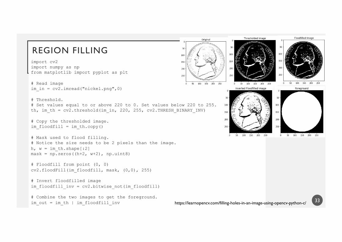
REGION FILLING
33
import cv2import numpy as npfrom matplotlib import pyplot as plt
# Read imageim_in = cv2.imread("nickel.png",0)
# Threshold.# Set values equal to or above 220 to 0. Set values below 220 to 255. th, im_th = cv2.threshold(im_in, 220, 255, cv2.THRESH_BINARY_INV)
# Copy the thresholded image.im_floodfill = im_th.copy()
# Mask used to flood filling.# Notice the size needs to be 2 pixels than the image.h, w = im_th.shape[:2]mask = np.zeros((h+2, w+2), np.uint8)
# Floodfill from point (0, 0)cv2.floodFill(im_floodfill, mask, (0,0), 255)
# Invert floodfilled imageim_floodfill_inv = cv2.bitwise_not(im_floodfill)
# Combine the two images to get the foreground.im_out = im_th | im_floodfill_inv https://learnopencv.com/filling-holes-in-an-image-using-opencv-python-c/
34
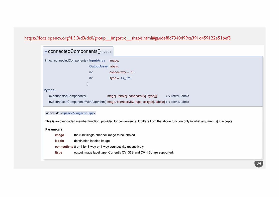
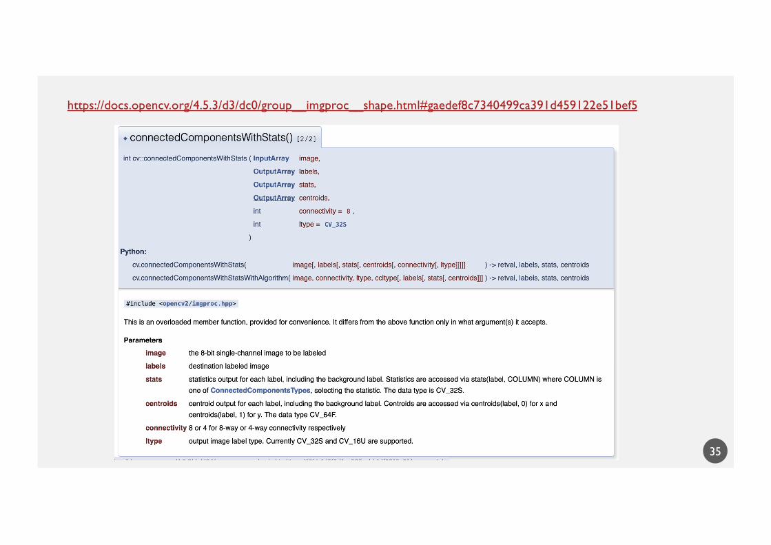
https://docs.opencv.org/4.5.3/d3/dc0/group__imgproc__shape.html#gaedef8c7340499ca391d459122e51bef5
35
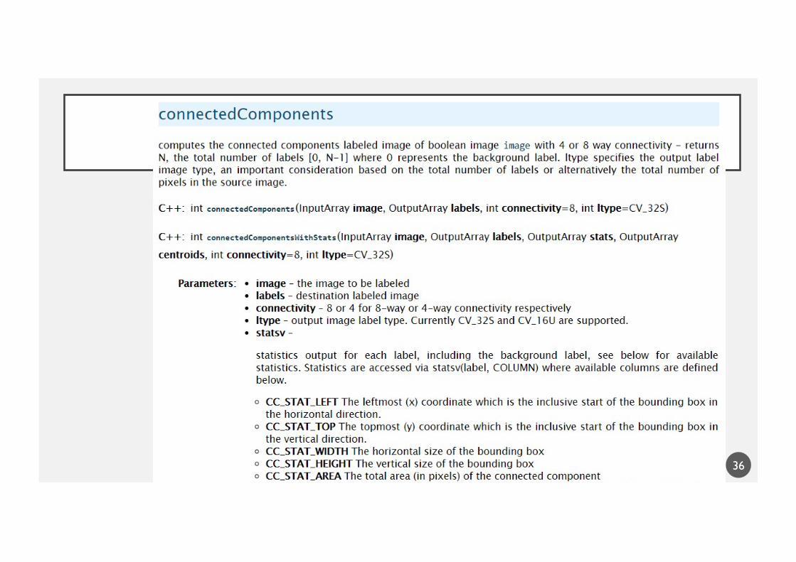
https://docs.opencv.org/4.5.3/d3/dc0/group__imgproc__shape.html#gaedef8c7340499ca391d459122e51bef5
36
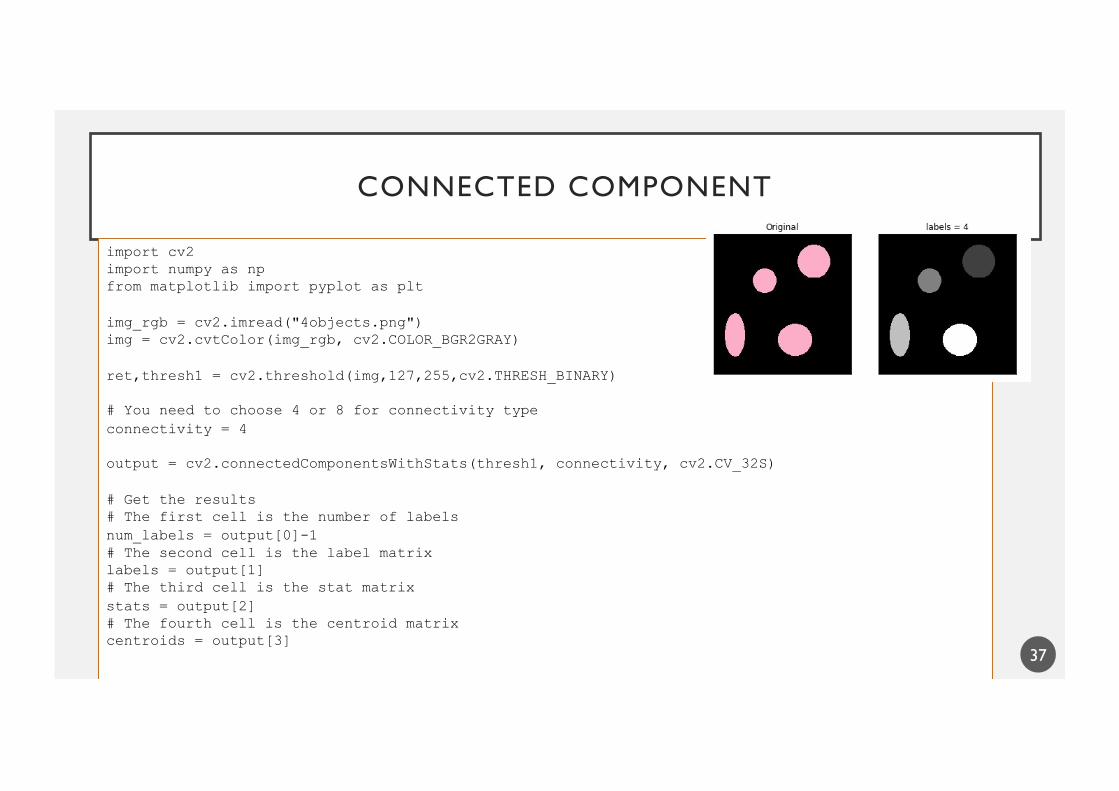
CONNECTED COMPONENT
37
import cv2import numpy as npfrom matplotlib import pyplot as plt
img_rgb = cv2.imread("4objects.png")img = cv2.cvtColor(img_rgb, cv2.COLOR_BGR2GRAY)
ret,thresh1 = cv2.threshold(img,127,255,cv2.THRESH_BINARY)
# You need to choose 4 or 8 for connectivity typeconnectivity = 4
output = cv2.connectedComponentsWithStats(thresh1, connectivity, cv2.CV_32S)
# Get the results# The first cell is the number of labelsnum_labels = output[0]-1# The second cell is the label matrixlabels = output[1]# The third cell is the stat matrixstats = output[2]# The fourth cell is the centroid matrixcentroids = output[3]
fig = plt.figure(figsize=(12,4))plt.subplot(121),plt.imshow(cv2.cvtColor(img_rgb, cv2.COLOR_BGR2RGB)),plt.title('Original')plt.xticks([]), plt.yticks([])label = 'labels = '+str(num_labels)plt.subplot(122),plt.imshow(output[1],cmap='gray'),plt.title(label)plt.xticks([]), plt.yticks([])plt.show()
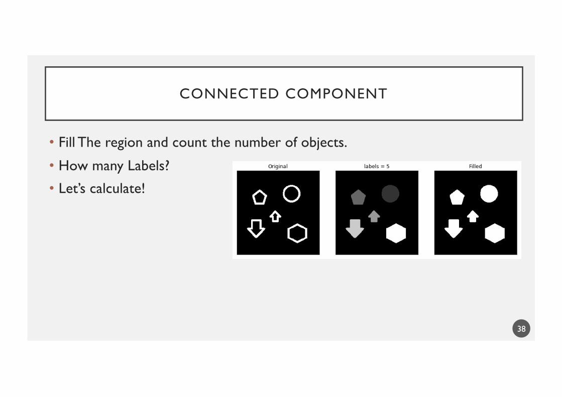
CONNECTED COMPONENT
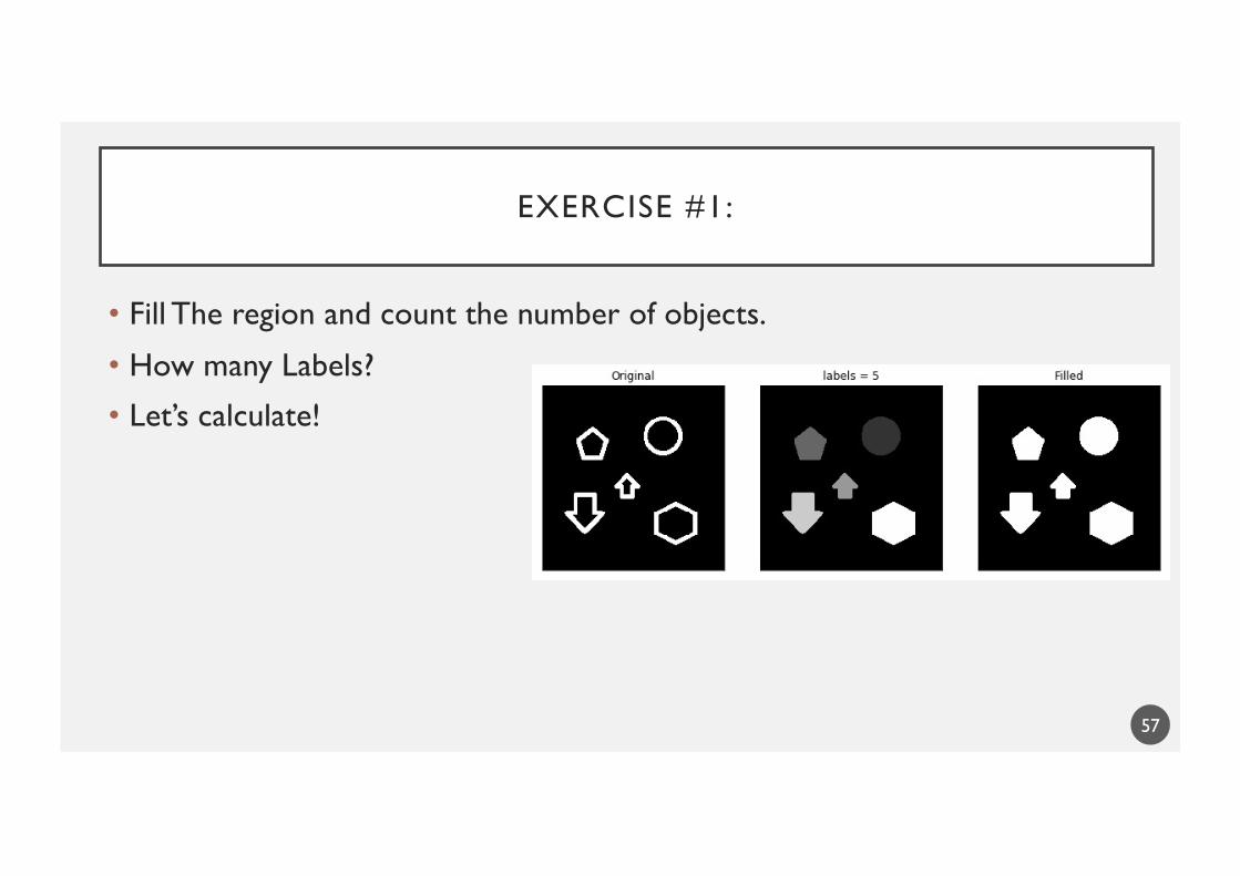
• Fill The region and count the number of objects.
• How many Labels?
• Let’s calculate!
38
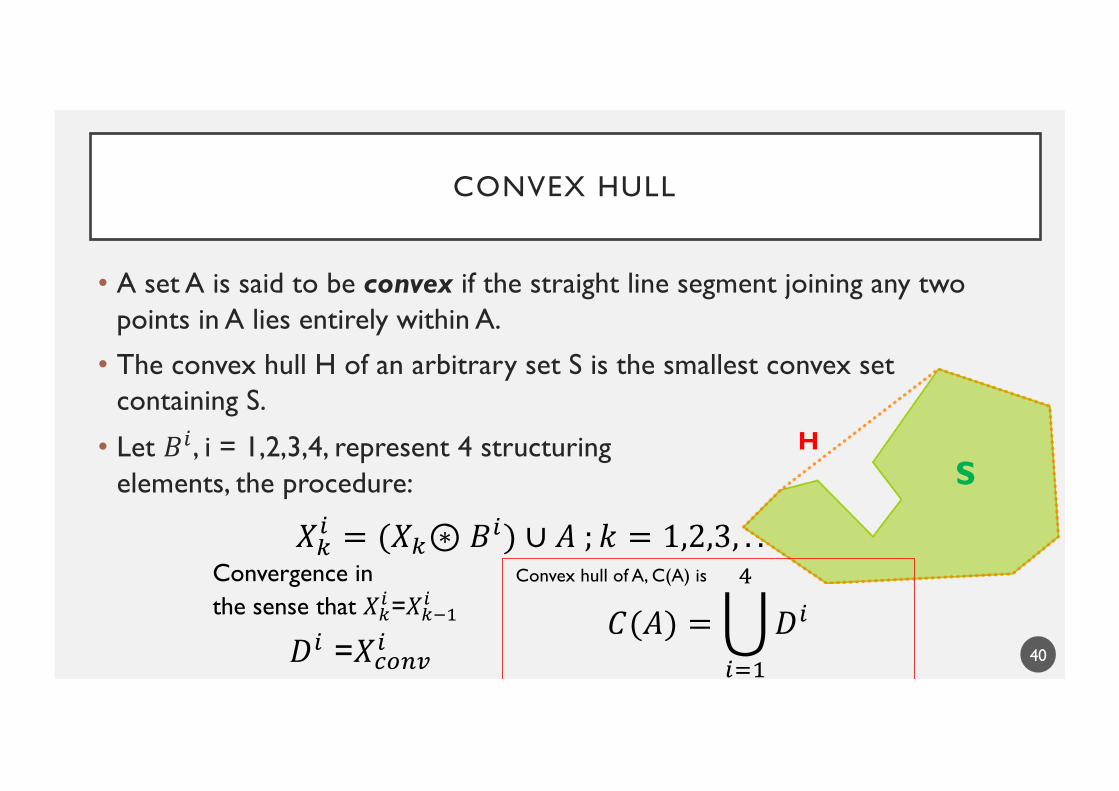
CONVEX HULL
• A set A is said to be convex if the straight line segment joining any two points in A lies entirely within A.
• The convex hull H of an arbitrary set S is the smallest convex set containing S.
• Let 𝐵' , i = 1,2,3,4, represent 4 structuringelements, the procedure:
40
HS
𝑋#& = (𝑋#⊛𝐵&) ∪ 𝐴 ; 𝑘 = 1,2,3, . .
𝐶(𝐴) =B&'%
(
𝐷&𝐷& =𝑋!)*+&
Convergence in the sense that 𝑋&'=𝑋&()'
Convex hull of A, C(A) is
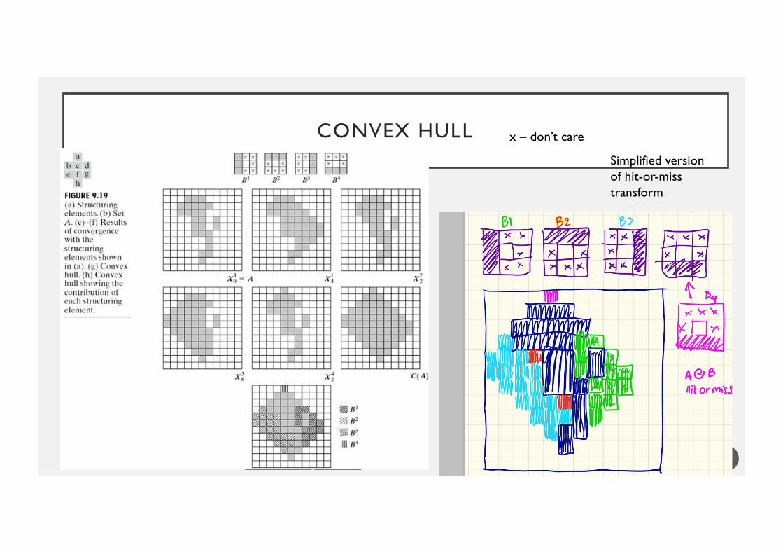
CONVEX HULL
41
Simplified version of hit-or-miss transform
x – don’t care
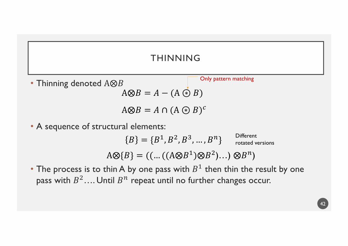
THINNING
• Thinning denoted A⨂𝐵
• A sequence of structural elements:
• The process is to thin A by one pass with 𝐵" then thin the result by one pass with 𝐵!…. Until 𝐵( repeat until no further changes occur.
42
A⨂𝐵 = 𝐴 − (A⊛ 𝐵)
A⨂𝐵 = 𝐴 ∩ (A⊛ 𝐵)$
𝐵 = {𝐵", 𝐵!, 𝐵), … , 𝐵(} Different rotated versions
Only pattern matching
A⨂{𝐵} = ((… ((A⨂𝐵")⨂𝐵!)…) ⨂𝐵()
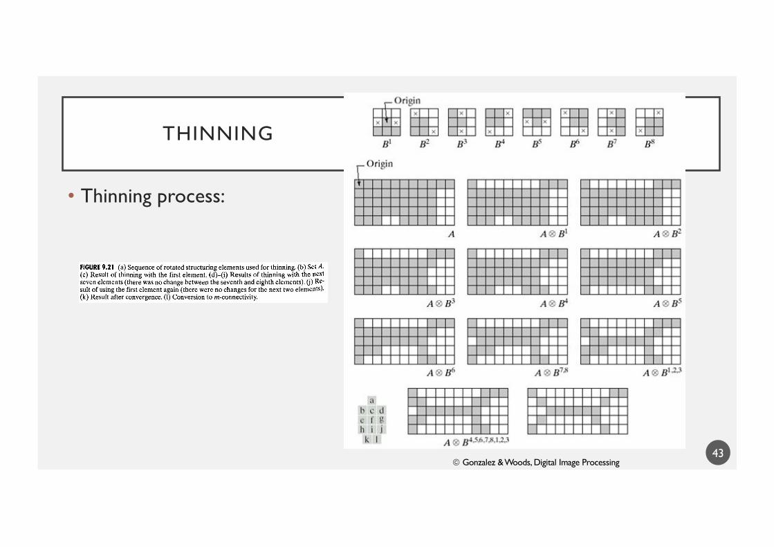
THINNING
• Thinning process:
43ã Gonzalez & Woods, Digital Image Processing
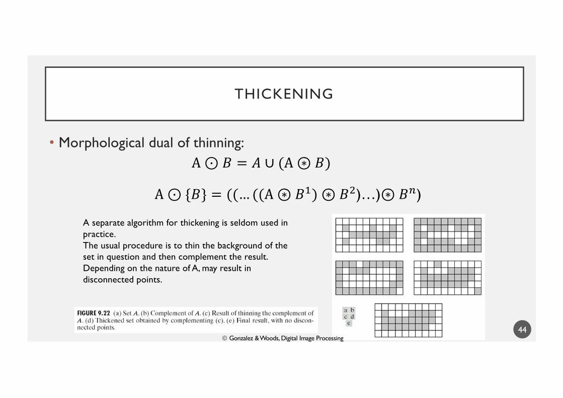
THICKENING
• Morphological dual of thinning:
44
A⊙ 𝐵 = 𝐴 ∪ (A⊛ 𝐵)
A⊙ {𝐵} = ((… ((A⊛ 𝐵") ⊛ 𝐵!)…)⊛𝐵()
A separate algorithm for thickening is seldom used in practice.The usual procedure is to thin the background of the set in question and then complement the result.Depending on the nature of A, may result in disconnected points.
ã Gonzalez & Woods, Digital Image Processing
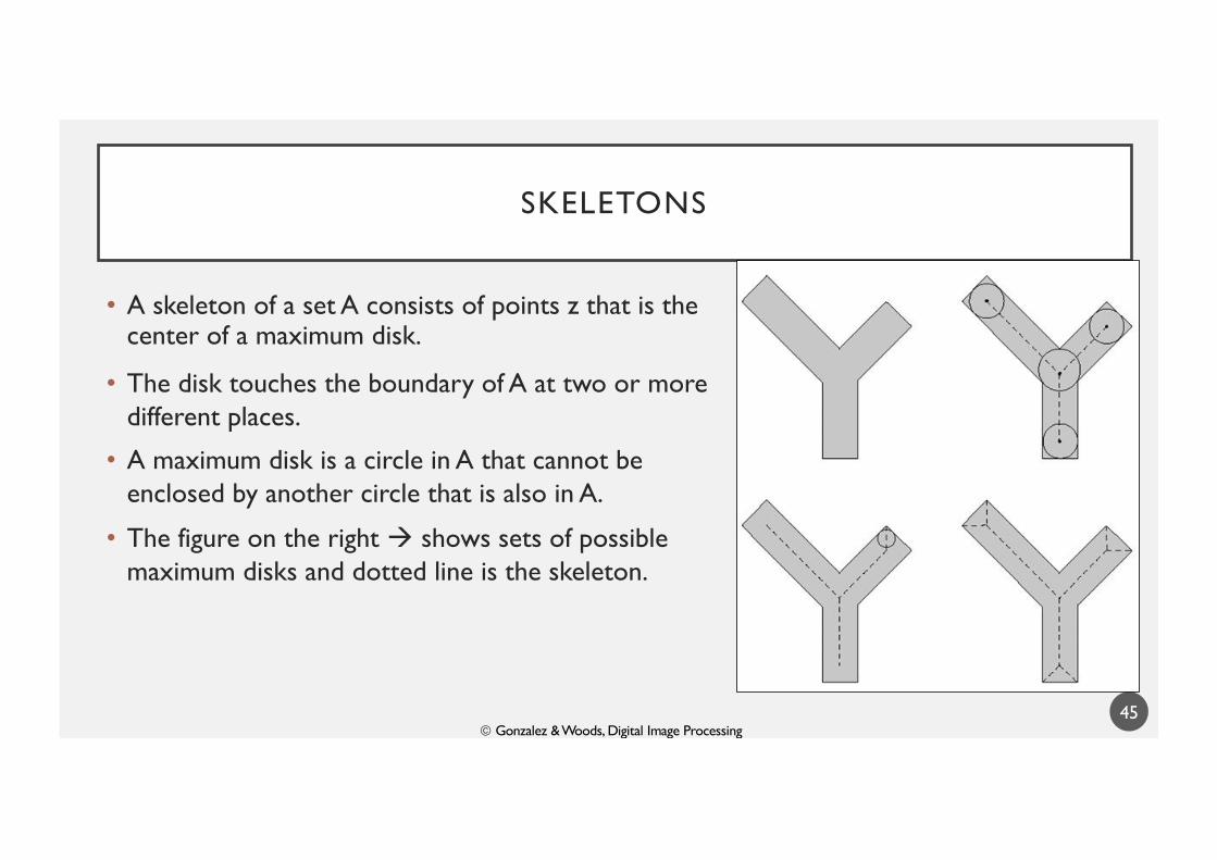
SKELETONS
• A skeleton of a set A consists of points z that is the center of a maximum disk.
• The disk touches the boundary of A at two or more different places.
• A maximum disk is a circle in A that cannot be enclosed by another circle that is also in A.
• The figure on the right à shows sets of possible maximum disks and dotted line is the skeleton.
45ã Gonzalez & Woods, Digital Image Processing
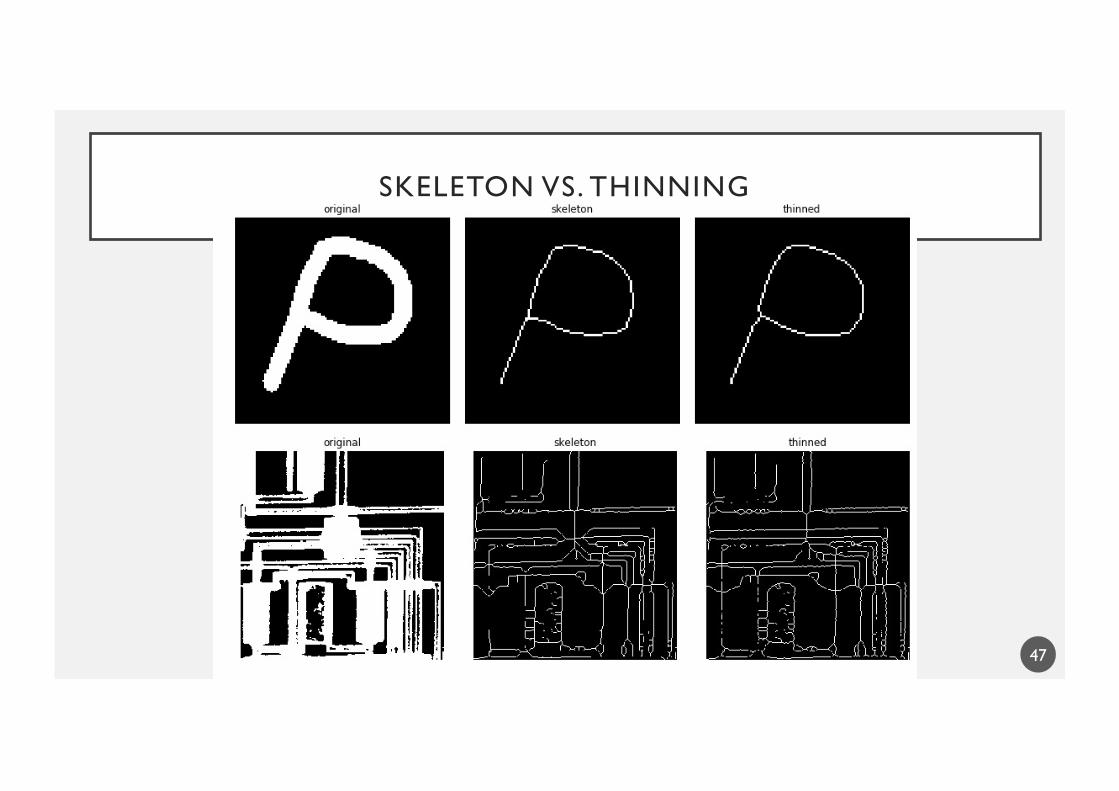
SKELETON VS. THINNING
47
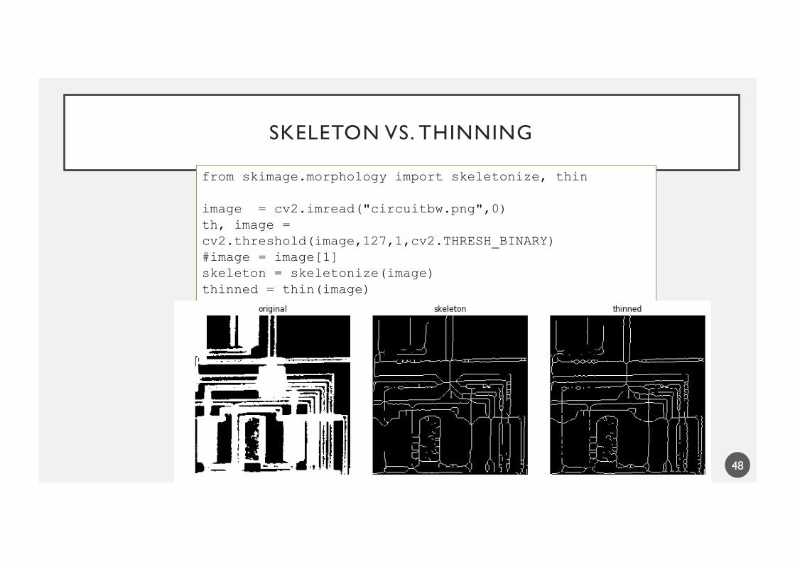
SKELETON VS. THINNING
48
from skimage.morphology import skeletonize, thin
image = cv2.imread("circuitbw.png",0)th, image = cv2.threshold(image,127,1,cv2.THRESH_BINARY)#image = image[1]skeleton = skeletonize(image)thinned = thin(image)
PRUNING
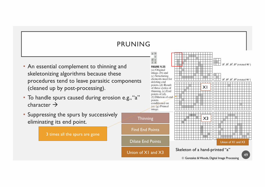
• An essential complement to thinning and skeletonizing algorithms because these procedures tend to leave parasitic components (cleaned up by post-processing).
• To handle spurs caused during erosion e.g., “a” character à
• Suppressing the spurs by successively eliminating its end point.
49Skeleton of a hand-printed “a”
Thinning
Find End Points
Dilate End Points
Union of X1 and X3
3 times all the spurs are gone
ã Gonzalez & Woods, Digital Image Processing
X1
X3
Union of X1 and X3
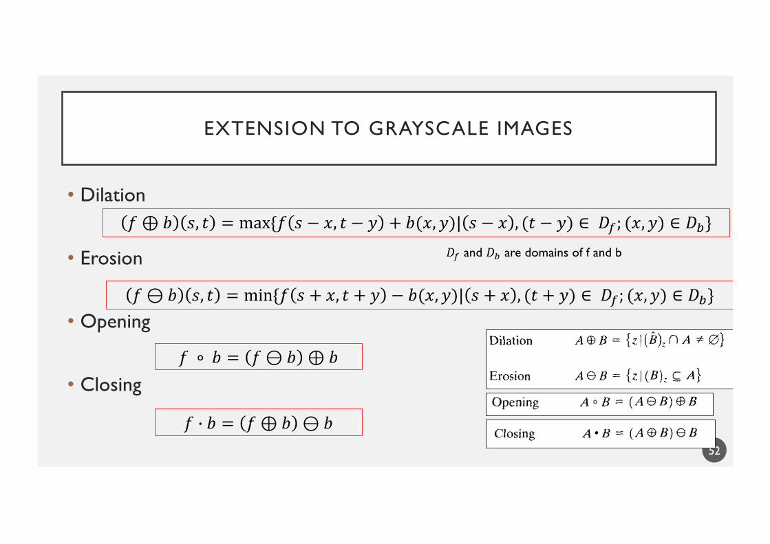
EXTENSION TO GRAYSCALE IMAGES
• Dilation
• Erosion
• Opening
• Closing
52
𝑓 ∘ 𝑏 = 𝑓 ⊖ 𝑏 ⊕ 𝑏
𝑓 ( 𝑏 = 𝑓 ⊕ 𝑏 ⊖ 𝑏
𝑓 ⊕ 𝑏 𝑠, 𝑡 = max{𝑓 𝑠 − 𝑥, 𝑡 − 𝑦 + 𝑏(𝑥, 𝑦)| 𝑠 − 𝑥 , (𝑡 − 𝑦) ∈ 𝐷*; (𝑥, 𝑦) ∈ 𝐷+}
𝑓 ⊖ 𝑏 𝑠, 𝑡 = min{𝑓 𝑠 + 𝑥, 𝑡 + 𝑦 − 𝑏(𝑥, 𝑦)| 𝑠 + 𝑥 , (𝑡 + 𝑦) ∈ 𝐷*; (𝑥, 𝑦) ∈ 𝐷+}
𝐷# and 𝐷$ are domains of f and b
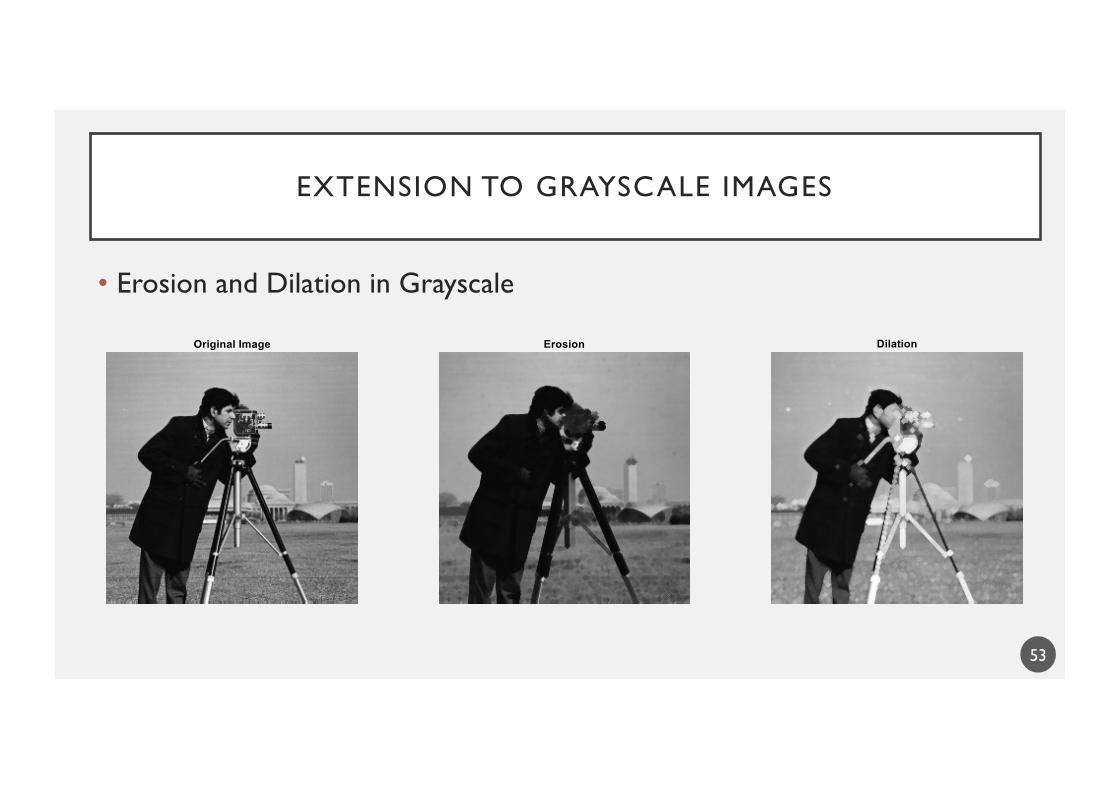
EXTENSION TO GRAYSCALE IMAGES
• Erosion and Dilation in Grayscale
53
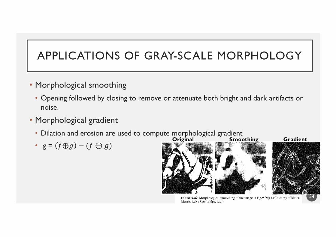
APPLICATIONS OF GRAY-SCALE MORPHOLOGY
• Morphological smoothing• Opening followed by closing to remove or attenuate both bright and dark artifacts or
noise.
• Morphological gradient• Dilation and erosion are used to compute morphological gradient
• g = 𝑓⨁𝑔 − (𝑓 ⊖ 𝑔)
54
Original Smoothing Gradient
APPLICATIONS OF GRAY-SCALE MORPHOLOGY
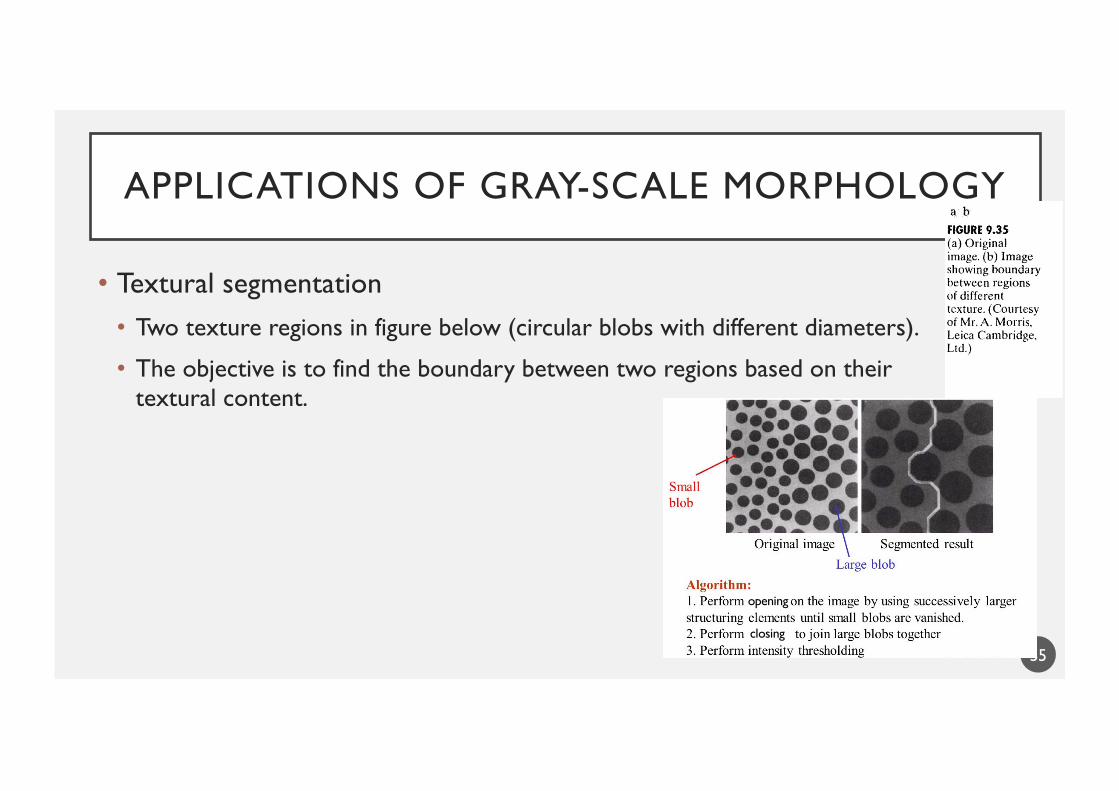
• Textural segmentation• Two texture regions in figure below (circular blobs with different diameters).
• The objective is to find the boundary between two regions based on theirtextural content.
55closing
opening
APPLICATIONS OF GRAY-SCALE MORPHOLOGY
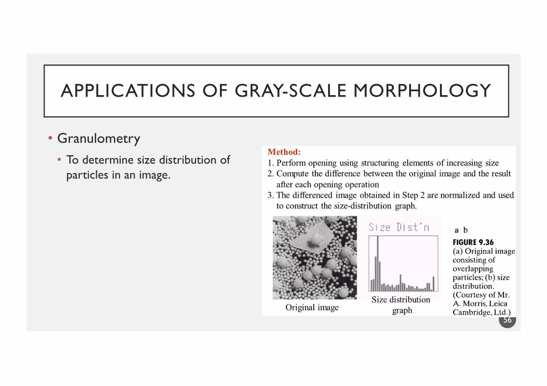
• Granulometry• To determine size distribution of
particles in an image.
56
EXERCISE #1:
• Fill The region and count the number of objects.
• How many Labels?
• Let’s calculate!
57
EXERCISE #2:
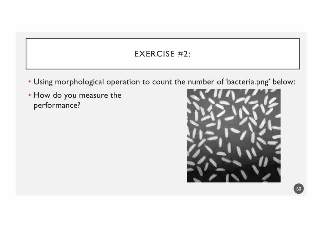
• Using morphological operation to count the number of ‘bacteria.png’ below:
• How do you measure the performance?
60
REFERENCES
• Rafael C. Gonzalez and Richard E. Woods, Digital Image Processing, Addison- Wesley• Chapter 9 Morphological Image Processing
61