lecnote fm surveying - carter center · pdf filefig. 4.7 hand level ... field book format for...
TRANSCRIPT

LECTURE NOTES
For Environmental Health Science Students
Surveying
Wuttiet Tafesse, Tesfaye Gobena
Haramaya University
In collaboration with the Ethiopia Public Health Training Initiative, The Carter Center, the Ethiopia Ministry of Health, and the Ethiopia Ministry of Education
2005

Funded under USAID Cooperative Agreement No. 663-A-00-00-0358-00.
Produced in collaboration with the Ethiopia Public Health Training Initiative, The Carter Center, the Ethiopia Ministry of Health, and the Ethiopia Ministry of Education.
Important Guidelines for Printing and Photocopying Limited permission is granted free of charge to print or photocopy all pages of this publication for educational, not-for-profit use by health care workers, students or faculty. All copies must retain all author credits and copyright notices included in the original document. Under no circumstances is it permissible to sell or distribute on a commercial basis, or to claim authorship of, copies of material reproduced from this publication.
©2005 by Wuttiet Tafesse, Tesfaye Gobena
All rights reserved. Except as expressly provided above, no part of this publication may be reproduced or transmitted in any form or by any means, electronic or mechanical, including photocopying, recording, or by any information storage and retrieval system, without written permission of the author or authors.
This material is intended for educational use only by practicing health care workers or students and faculty in a health care field.
i
Preface
This lecture note is prepared for Environmental Health
Science Students who need to understand measurement of
distances, angles and other similar activities. It is designed to
give the student the basic concepts and skills of surveying for
undergraduate level. This material could have paramount
importance for the health professionals who are involved in
public health activities.
Public health students are frequently involved in community
diagnosis, one of the major activities of public health. This
activity requires, among other things, drawing of sketch maps
of the area in question. A basic knowledge of surveying is of
great help for planning, designing, layout and construction of
different sanitary facilities.
In Ethiopia there are no textbooks, which could appropriately
fulfill the requirements of surveying course for Environmental
Health Science students. We believe that this lecture note can
fill that gap.
This lecture note is divided in to nine chapters. Each chapter
comprises of learning objectives, introduction, and practical
exercises.
ii
Acknowledgement
We would like to acknowledge The Carter Center for the
financial sport to the workshop conducted to develop the
lecture note. We would also like to thank Alemaya University,
Faculty of Health Sciences academic staff members for
reviewing the manuscript in the intra-institutional workshop.
Our deep appreciation also goes to Essayas Alemayehu , Ato
Zeleke Alebachew , Ato adane Sewuhunegn, Ato Embialle
Mengistie and Ato Yonas Mamo who gave valuable
comments during the inter-institutional workshop.
iii
Table of Contents Preface ........................................................................ i
Acknowledgement ........................................................ ii
Table of Contents ......................................................... iii
List of figures ................................................................ vi
Acronyms ..................................................................... ix
CHAPTER ONE: Introduction To Surveying 1.1. Learning objectives ......................................... 1 1.2. Introduction ..................................................... 1 1.3. Definition and Technical Terms ...................... 2 1.4. Importance of surveying ................................. 2 1.5. Application of Surveying in Environmental Health Activities ..................................................... 3 Exercise ................................................................. 4
CHAPTER TWO: The Basic Surveying Methods 2.1. Learning Objectives ........................................ 5 2.2. Introduction ..................................................... 5 2.3. Measuring Distances and Angles ................... 7 2.4. Types of Surveying ......................................... 9 2.5. Surveying Applications ................................... 11 2.6. Field Notes ...................................................... 14 Exercise ................................................................. 15
CHAPTER THREE: Measurements and Computations 3.1. Learning Objectives ........................................ 16 3.2. Introduction ..................................................... 16 3.3. Types of Measurements in Surveying ............ 17
iv
3.4. Significant Figures .......................................... 20 3.5. Mistakes and Errors ........................................ 23 3.6. Accuracy and Precision .................................. 29 Exercise ................................................................. 34
CHAPTER FOUR: Measuring Horizontal Distances 4.1. Learning Objectives ........................................ 37 4.2. Introduction ..................................................... 37 4.3. Rough Distance Measurement ....................... 38 4.4. Taping Equipments and Methods ................... 41 Exercise ................................................................. 57
CHAPTER FIVE: Leveling 5.1. Learning Objectives ........................................ 60 5.2. Introduction ..................................................... 60 5.3. Measuring Vertical Distances ......................... 61 5.4. Methods of Leveling ....................................... 61 5.5. Benchmarks and Turning Points .................... 65 5.6. Inverted Staff Reading .................................... 68 5.7. Reciprocal Leveling ........................................ 69 5.8. Leveling Equipment ........................................ 70 5.9. Leveling Procedures ....................................... 76 5.10. Profit Leveling ............................................... 90 5.11. Cross-Section Leveling ................................. 93 5.12. Three-Wire Leveling ..................................... 95 Exercise ................................................................. 97
CHAPTER SIX: Tachometry 6.1. Learning Objectives ........................................ 102 6.2. Introduction ..................................................... 102 6.3. Principles of Stadia ......................................... 102 6.4. Stadia Measurement on an inclined Sights .... 105
v
6.5. Sources of Errors in Stadia Work ................... 108 Exercise ................................................................. 110
CHAPTER SEVEN: Angles, Bearing and Azimuths 7.1. Learning objectives ......................................... 112 7.2. Introduction ..................................................... 112 7.3. Angles ............................................................. 112 7.4. Direction of a Line ........................................... 117 7.5. Azimuths ......................................................... 120 7.6. Compass Survey ............................................ 124 Exercise ................................................................. 128
CHAPTER THREE: Traversing 8.1. Learning Objectives ........................................ 130 8.2.Introduction ...................................................... 130 8.3 Balancing Angles ............................................. 132 8.4. Latitudes and Departures ............................... 133 8.5 Traverse Adjustment ....................................... 136 8.6 Application Of Traversing ................................ 138 Exercise Error! Bookmark Not Defined ................. 145
CHAPTER NINE: Construction Surveys 9.1 Learning Objectives ......................................... 150 9.2. Introduction ..................................................... 150 9.3. Setting out a Peg on a Specified Distance and
Bearing ............................................................ 154 9.4. Setting Out Small Buildings ............................ 158 9.5. Sewer and Tunnel Construction ..................... 168 Exercise ................................................................. 172
GLOSSARY ................................................................. 173
REFERENCES ............................................................. 180

vi
LIST OF FIGURES Fig. 2.1 Shape of the earth ........................................... 6 Fig. 2.2 The vertical direction ....................................... 7 Fig. 2.3 A true horizontal distance; is actually curved,
like the surface of the earth ............................. 8 Fig. 2.4 Plane surveying ............................................... 10 Fig. 3.1 Steel tape ........................................................ 18 Fig. 3.2 Illustration of accuracy and precision .............. 21 Fig. 3.3 Illustration of accuracy and precision .............. 30 Fig. 4.1 Pacing provides a simple yet useful way
to make distance measurement ...................... 39 Fig. 4.2 A typical measuring wheel used for making
rough distance measurements ........................ 40 Fig. 4.3 Fiber glass tapes (A) closed caes; (B)
Open reel ........................................................ 42 Fig. 4.4 A pulb bob is one of the simplest yet most
important acessories for accurate surveying .. 43 Fig. 4.5 A surveyor's range pole .................................. 43 Fig. 4.6 (a) Chaining pin (b) Keel ................................. 44 Fig. 4.7 Hand level ....................................................... 44 Fig. 4.8 ........................................................................ 45 Fig. 4.9 A tape clamp handle ....................................... 46 Fig. 4.10 Breaking tape ................................................ 47 Fig. 5.1 Differential leveling to measure vertical distance
and elevation. (a) Step 1: take a back sight rod reading on point A (b) Step 2: rotate the telescope toward point Band take foresight rod reading ...................................................... 63
vii
Fig. 5.2 Temporary turning points are used to carry a
line of levels from a benchmark to some other station or benchmark; the process of differential leveling is repeated each instrument set up.... 65
Table 5.1. Field book format for leveling notes ............ 67 Fig. 5.3 Illustration of inverted staff reading ................. 68 Table 5.2. Shows the reading observed to the points
A, B, C, and D on the multistory building of figure 5.3 -Illustration of inverted staff reading 69
Fig 5.4 Dumpy level ..................................................... 71 Fig 5.5 Tilting level ....................................................... 71 Fig 5.6 Automatic levels ............................................... 72 Fig.5.7 traditional rectangular cross section leveling
rods showing a variety of graduation markings 75 Fig. 5.8 Circular rod level ............................................. 76 Fig. 5.9 Tripod stands .................................................. 77 Fig. 5.10 tripod head adaptor ....................................... 77 Fig 5.11 Leveling a three-screw instrument ................. 78 Fig 5. 12. When the horizontal length of the foresight
(plus) and backsight (minus) are the same, the systematic error of adjustment of the level is cancelled ............................................. 81
Fig. 5.13 Illustration of horizontal line and level surface departure. ........................................................ 82
Fig. 6.1 Horizontal stadia measurement ...................... 103 Fig. 6.2. Inclined Stadia measurement ........................ 105 Fig. 7.1. The three determinants of an angle ............... 113 Fig. 7.2. Theodlites ....................................................... 114
viii
Fig. 7.3. Horizontal circle reading using optical
micrometer ...................................................... 115 Fig. 7.4. Interior angles of a polygon ............................ 116 Fig. 7.5. Angles of the right .......................................... 116 Fig. 7.6. Deflection angles ............................................ 117 Fig.7.7 The bearing of a line is measured from the north
or from the south ............................................. 119 Fig. 7.8 Bearings .......................................................... 120 Fig 7.9 Azimuths .......................................................... 121 Fig. 7.10 Bearings and angles ..................................... 123 Fig. 7.11Declination east .............................................. 125 Fig. 7.12 Declination set off on a compass circle ........ 125 Fig. 8.1 Open traverse ................................................. 131 Fig. 8.2 Closed traverse ............................................... 132 Fig. 8.3 latitude and Departure .................................... 135 Fig. 8.4 Area by rectangular coordinates ..................... 140 Fig. 8.5 Meridian distances and areas ......................... 141 Fig. 8.6 Area by double meridian distances ................. 142 Fig. 9.1. Setting out pegs and profiles ......................... 153 Fig 9.2. Setting out on level ground ............................. 155 Fig 9.3. Setting out small buildings .............................. 159 Fig. 9.4. Setting out the building .................................. 162 Fig. 9.5. Setting out instrument on sloping ground ...... 163 Fig. 9.6. Setting out peg at a predetermined level ....... 165

ix
ACRONYMS
BM: Bench Mark
EDM: Electronic Distance Measurement
HI: Height of Instrument above a datum
hi: Height of Instrument(optical axis) above the
instrument station
TP: Turning point
DMD: Double Meridian Distance
MSL: Mean Sea Level
FS: Foresight
BS: Backsight
1
CHAPTER ONE INTRODUCTION TO SURVEYING
1.1. LEARNING OBJECTIVES At the end of this chapter, students will be able to:
1. Define surveying and other technical terms
2. Describe the importance of surveying
3. know the application of surveying in environmental
health activities.
1.2 INTRODUCTION Surveying has been important since the beginning of
civilization. Today, the importance of measuring and
monitoring our environment is becoming increasingly critical
as our population expands, land values appreciates, our
natural resources dwindle, and human activities continue to
pollute our land, water and air. As a result, the breadth and
diversity of practice of surveying, as well as its importance in
modern civilization is increasing from time to time.
Surveying is a discipline, which encompasses all methods for measuring, processing, and disseminating
information about the physical earth and our environment.
2
1.3 Definition and Technical Terms Simply stating, surveying involves the measurement of
distances and angles. The distance may be horizontal or
vertical in direction. Vertical distances are also called
elevations. Similarly, the angles may be measured in
horizontal and vertical plane. Horizontal angles are used to
express the directions of land boundaries and other lines.
There are two fundamental purposes for measuring distances
and angles.
The first is to determine the relative positions of existing
points or objects on or near the surface of the earth.
The second is to layout or mark the desired positions of
new points or objects, which are to be placed or
constructed on or near the surface of the earth.
Surveying measurements must be made with precision in
order to achieve a maximum of accuracy with a minimum
expenditure of time and money.
The practice of surveying is an art, because it is dependent
up on the skills, judgments and experience of surveyor. It may
also be considered as an applied science, because field and
office procedures rely upon a systematic body of knowledge.
1.4 IMPORTANCE OF SURVEYING Surveying is one of the world’s oldest and most important arts
because, as noted previously, from the earliest times it has

3
been necessary to mark boundaries and divide land.
Surveying has now become indispensable to our modern way
of life. The results of today’s surveys are being used to:
1. Map the earth above and below sea level.
2. Prepare navigational carts for use in the air, on land
and at sea.
3. Establish property boundaries of private and public
lands
4. Develop data banks of land-use and natural
resources information which aid in managing our
environment
5. Determine facts on the size, shape, gravity and
magnetic fields of the earth and
6. Prepare charts of our moon and planets.
1.5 Application of Surveying in Environmental Health Activities
Surveying plays an essential role in the planning, design,
layout, and construction of our physical environment and
infrastructure (all the constructed facilities and systems which
human communities use to function and thrive productivity). It
is also the link between design and construction. Roads,
bridges, buildings, water supply, sewerage, drainage systems,
and many other essential public work projects could never
have been built without surveying technology.
4
Exercise
1. Give a brief definition of Surveying.
2. Describe the two fundamental purposes of surveying.
3. Briefly describe why surveying may be characterized as
both an art and a science.
4. Why is surveying an important technical discipline?
5. Discuss the application of surveying in environmental
health activities.
5
CHATER TWO THE BASIC SURVEYING METHODS
2.1 LEARNING OBJECTIVES At the end of this chapter, students will be able to:
1. Identify and state the different types of surveying
2. Describe different surveying applications
3. Apply measurement of distances and angles
4. Describe the rules of field notes of a surveyor.
2.2 INTRODUCTION Most surveying activities are performed under the pseudo
assumption that measurements are being made with
reference to a flat horizontal surface. This requires some
further explanation.
The earth actually has the approximate shape of a spheroid
that is the solid generated by an ellipse rotated on its minor
axis. However, for our purposes, we can consider the earth to
be a perfect sphere with a constant diameter. In addition, we
can consider that the average level of the ocean or mean sea
levels represent the surface of sphere.
6
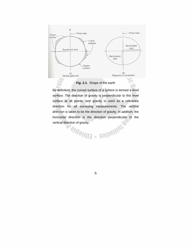
Fig. 2.1. Shape of the earth
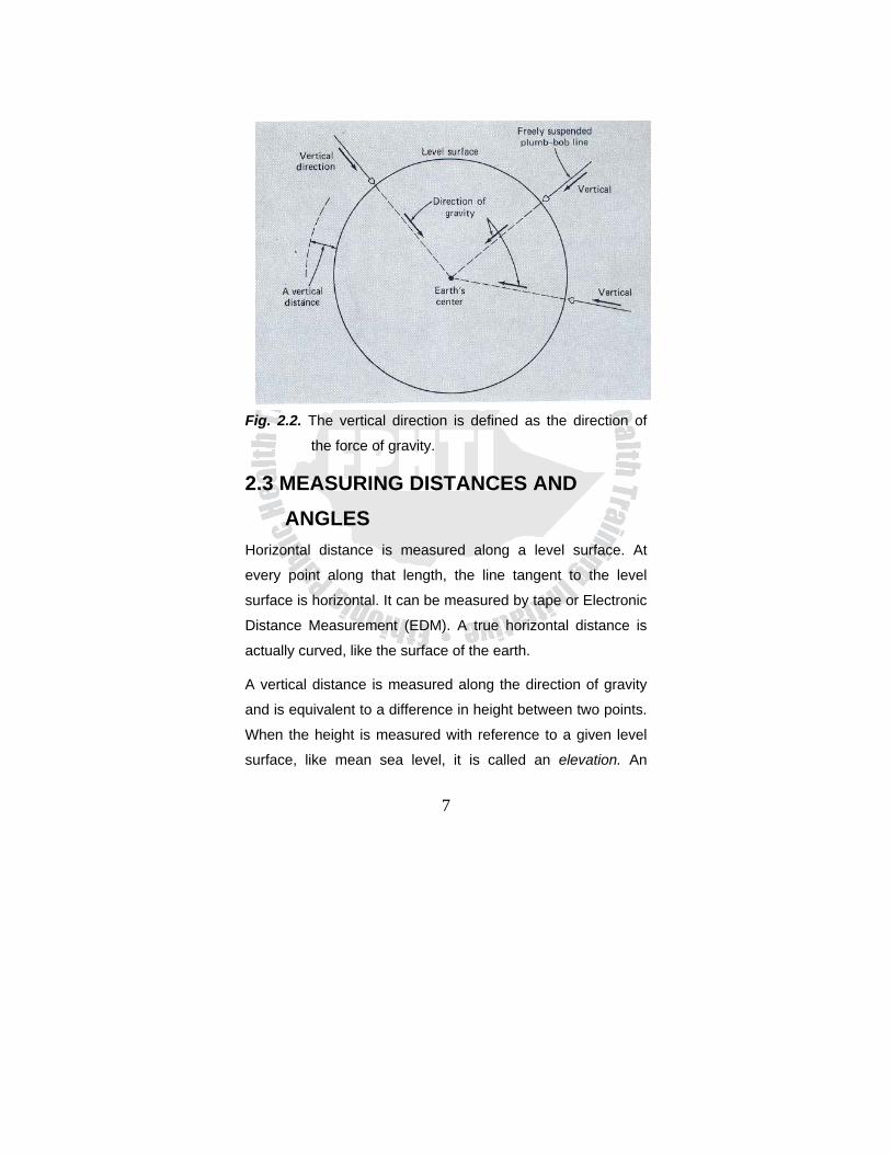
By definition, the curved surface of a sphere is termed a level
surface. The direction of gravity is perpendicular to this level
surface at all points, and gravity is used as a reference
direction for all surveying measurements. The vertical
direction is taken to be the direction of gravity. In addition, the
horizontal direction is the direction perpendicular to the
vertical direction of gravity.
7
Fig. 2.2. The vertical direction is defined as the direction of
the force of gravity.
2.3 MEASURING DISTANCES AND ANGLES
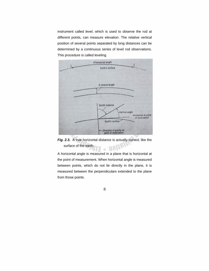
Horizontal distance is measured along a level surface. At
every point along that length, the line tangent to the level
surface is horizontal. It can be measured by tape or Electronic
Distance Measurement (EDM). A true horizontal distance is
actually curved, like the surface of the earth.
A vertical distance is measured along the direction of gravity
and is equivalent to a difference in height between two points.
When the height is measured with reference to a given level
surface, like mean sea level, it is called an elevation. An
8
instrument called level, which is used to observe the rod at
different points, can measure elevation. The relative vertical
position of several points separated by long distances can be
determined by a continuous series of level rod observations.
This procedure is called leveling.
Fig. 2.3. A true horizontal distance is actually curved, like the
surface of the earth.
A horizontal angle is measured in a plane that is horizontal at
the point of measurement. When horizontal angle is measured
between points, which do not lie directly in the plane, it is
measured between the perpendiculars extended to the plane
from those points.
9
A vertical angle is measured in a plane that is vertical at the
point of observation or measurement. Horizontal and vertical
angles are measured with an instrument called a transit or
theodolite.
2.4 Types of Surveying
There are two types of surveying: these are
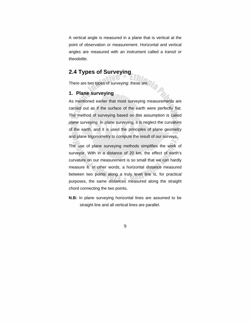
1. Plane surveying As mentioned earlier that most surveying measurements are
carried out as if the surface of the earth were perfectly flat.
The method of surveying based on this assumption is called
plane surveying. In plane surveying, it is neglect the curvature
of the earth, and it is used the principles of plane geometry
and plane trigonometry to compute the result of our surveys.
The use of plane surveying methods simplifies the work of
surveyor. With in a distance of 20 km, the effect of earth’s
curvature on our measurement is so small that we can hardly
measure it. In other words, a horizontal distance measured
between two points along a truly level line is, for practical
purposes, the same distances measured along the straight
chord connecting the two points.
N.B: In plane surveying horizontal lines are assumed to be
straight line and all vertical lines are parallel.
10
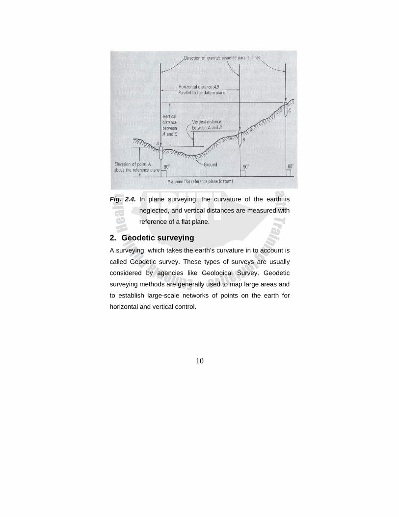
Fig. 2.4. In plane surveying, the curvature of the earth is
neglected, and vertical distances are measured with
reference of a flat plane.
2. Geodetic surveying A surveying, which takes the earth’s curvature in to account is
called Geodetic survey. These types of surveys are usually
considered by agencies like Geological Survey. Geodetic
surveying methods are generally used to map large areas and
to establish large-scale networks of points on the earth for
horizontal and vertical control.
11
2.5 SURVEYING APPLICATIONS As mentioned earlier, the two fundamental purposes for
surveying are to determine the relative positions of existing
points and to mark the positions of new points on or near the
surface of the earth. However, different types of surveys
require different field procedures and varying degrees of
precision for carrying out the work.
• Property survey It is also called land survey or boundary survey. It is
performed in order to establish the positions of boundary lines
and property corners. It is usually performed whenever land
ownership is to be transferred or when a large tract of land is
to be subdivided in to smaller parcels for development. It is
also performed before the design and construction of any
public/private land-use project.
• Topographic survey It is performed in order to determine the relative positions of
existing natural and constructed features on a tract of land
(like ground elevation, bodies of water, roads, buildings etc.).
It provides information on the “shape of the land” hills, valleys,
ridges and general slope of the ground. The data’s obtained
from a topographic surveys are plotted in a map called
topographic map and the shape of the ground is shown with
lines of equal elevation called contours.
12
• Construction survey It is also called layout or location survey and performed in
order to mark the positions of new points on the ground.
These new points represent the location of building corners,
road centerlines and other facilities that are to be built.
• City survey The surveys which are carried out for the construction of
roads, parks water supply system, sewer and other
constructional work for any developing township, are called
city surveys. The city maps which are prepared for tourists are
known as guide maps.
• Control survey
There are two kinds of control surveys: These are horizontal
and vertical control survey.
1. Horizontal control survey:
The surveyor, using temporary/permanent markers, places
several points in the ground. These points, called stations, are
arranged through out the site area under study so that it can
be easily seen.
The relative horizontal positions of these points are
established, usually with a very high degree of precisions and
accuracy; this is done using transverse, triangulation or
trilateration methods.
13
2. Vertical control survey
The elevations of relatively permanent reference points are
determined by precise leveling methods. Marked points of
known elevations are called elevation benchmarks. The
network of stations and benchmarks provide a framework for
horizontal and vertical control, up on which less accurate
surveys can be based.
• Route survey It is performed in order to establish horizontal and vertical
controls, to obtain topographic data, and to layout the position
of high ways, railroads, pipe lines etc. The primary aspect of
route surveying is that the project area is very narrow
compared with its length, which can extend for many
kilometers.
• Other types of surveys HYRDRAULIC SURVEY: is a preliminary survey
applied to a natural body of water, e.g. mapping of
shorelines, harbor etc.
RECONNAISSANCE SURVEY: is a preliminary
survey conducted to get rough data regarding a tract
of land.
PHOTOGRAMMETRIC SURVEYING: uses relatively
accurate methods to convert aerial photographs in to
useful topographic maps.

14
2.5 FIELD NOTES All surveys must be free from mistakes or blunders. A
potential source of major mistakes in surveying practice is the
careless or improper recording of field notes. The art of
eliminating blunders is one of the most important elements in
surveying practice.
RULES FOR FIELD NOTES 1. Record all field data carefully in a field book at the moment they are
determined.
2. All data should be checked at the time they are recorded.
3. An incorrect entry of measured data should be neatly lined out, the
correct number entered next to or above it.
4. Field notes should not be altered, and even data that are crossed out
should still remain legible.
5. Original field records should never be destroyed, even if they are
copied for one reason to another.
6. A well-sharpened medium-hard pencil should be used for all field
notes.
7. Sketches should be clearly labeled.
8. Show the word VOID on the top of pages that, for one reason or
another, are invalid.
9. The field book should contain the name, address, and the phone
number.
10. Each new survey should begin on a new page.
11. For each day of work, the project name, location, and date should be
recorded in the upper corner of the right –hand page.
15
Exercise
1. Define and briefly discuss the terms vertical and
horizontal distance and angle.
2. Is a horizontal distance a perfect straight line? Why?
3. What is meant by the term elevation?
4. What does the term leveling mean?
5. What surveying instruments are used to measure angles
and distances?
6. What is the basic assumption for plane surveying?
7. How does geodetic surveying differ from plane surveying?
8. Under what circumstances is it necessary to conduct a
geodetic survey?
9. Give a brief description of the topographic and
construction surveying.
10. Why is the proper recording of field notes a very important
part of surveying practice?
16
CHAPTER THREE MEASUREMENTS AND COMPUTATIONS
3.1 LEARNING OBJECTIVES At the end of this chapter, the student will be able to:
1. Describe types of measurement in surveying
2. State the different types of errors in surveying
3. Identify and select instruments and procedures
necessary to reduce errors
3.2 INTRODUCTION Making measurements and subsequent computations and
analyses using them are fundamental tasks of surveyors. The
process requires a combination of human skill and mechanical
equipment applied with the utmost judgment. No matter how
carefully made, however, measurements are never exact and
will always contain errors.
Surveyors, whose work must be performed to exacting
standards, should therefore thoroughly understand the
different kinds of errors, their sources and expected
magnitudes under varying conditions, and their manner of
propagation. Only then can they select instruments and
procedures necessary to reduce error sizes to within tolerable
limits.
17
3.3 TYPES OF MEASURMENTS IN SURVEYING
There are five basic kinds of measurements in plane
surveying:
1. Horizontal angles
2. Horizontal distance
3. Vertical angles
4. Vertical distance
5. Slope distance
By using combinations of these basic measurements it is
possible to compute relation positions between any points.
Measurement of distances and angles it is the essence
surveying.
Angle is simply figure formed by the intersection of two lines
or figures generated by the rotation of a line about a point
form an initial position to a terminal position. The point of
rotation is colled the vertex of the angle.
There are several systems of angle measurement. The most
common ones are sexagesimal system and centesimal
system
18
A. The Sexagesimal System: This system uses degrees, minutes
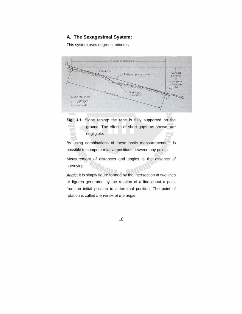
Fig. 3.1. Slope taping: the tape is fully supported on the
ground. The effects of short gaps, as shown, are
negligible.
By using combinations of these basic measurements it is
possible to compute relative positions between any points.
Measurement of distances and angles is the essence of
surveying.
Angle: it is simply figure formed by the intersection of two lines
or figures generated by the rotation of a line about a point
from an initial position to a terminal position. The point of
rotation is called the vertex of the angle.
19
There are several systems of angle measurement. The most
common ones are sexagesimal system and centesimal
system
This system uses degrees, minutes and seconds. In this
system, a complete rotation of a line (circle) is divided in to
360 degrees of arc. One degree is divided in to 60 minutes
and 1 minute is further divided in to 60 seconds of arc. The
symbols for degree, minutes and seconds are 0, ’ and ’’ respectively.
E.g. 350 17’46’’
900, 00’ 00’’
One can perform additions, subtractions and conversions in
the sexagesimal system as follows:
+ 35017’46’’ - 90000’00’’
25047’36 35017’46’’
60064’82’’ = 61 005’22’’ 54042’14’’
Conversion 35030’ = 35.50
142.1250 = 142007’30’’
20
B. The Centesimal System This system uses the grad for angular measurement. Here, a
complete rotation is divided in to 400 grads. The grad is sub
divided in to 100 parts called centigrad and the centigrad is
further sub divided in to100 centi-centigrad (1c =100cc)
For conversion 1g = 0.90
Example. 100 grad = 90 degrees
3.4. SIGNIFICANT FIGURES A measured distance or angle is never exact; the “true’ or
actual value can not be determined primarily because there is
no perfect measuring instrument. The closeness of the
observed value to the true value depends up on the quality of
the measuring instrument and the care taken by the surveyor.
The number of significant figures in a measured quantity is the
number of sure or certain digits, plus one estimated digit. This
is a function primarily of the least count or graduation of the
measuring instrument.
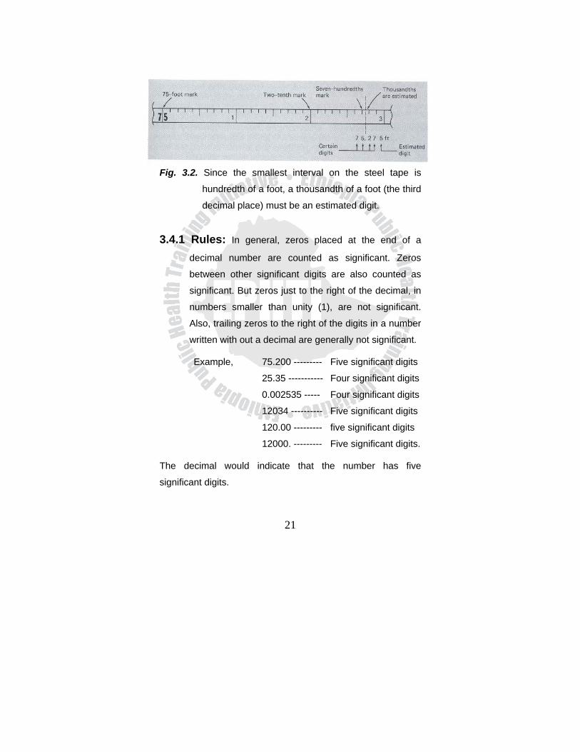
For example, an observed distance of 75.2 ft has three
significant figures. It would be incorrect to report the distance
as 75.200 ft (five significant digits), since that would imply a
greater degree of exactness than can be obtained with the
measuring instrument.
21
Fig. 3.2. Since the smallest interval on the steel tape is
hundredth of a foot, a thousandth of a foot (the third
decimal place) must be an estimated digit.
3.4.1 Rules: In general, zeros placed at the end of a
decimal number are counted as significant. Zeros
between other significant digits are also counted as
significant. But zeros just to the right of the decimal, in
numbers smaller than unity (1), are not significant.
Also, trailing zeros to the right of the digits in a number
written with out a decimal are generally not significant.
Example, 75.200 --------- Five significant digits
25.35 ----------- Four significant digits
0.002535 ----- Four significant digits
12034 ---------- Five significant digits
120.00 --------- five significant digits
12000. --------- Five significant digits.
The decimal would indicate that the number has five
significant digits.
22
But in this case, it would be preferable to use scientific
notation, that is, 1.2 × 10⁴, to indicate the significance of the
trailing zeros.
When numbers representing measured quantities are added,
the sum cannot be any more exact than any of the original
numbers. The least numbers of decimals is generally the
controlling factor.
E.g., 4.52 + 23.4 + 468.321 = 496.241 rounded off to
496.2
When subtracting one number from another, it is best first to
round off to the same decimal place.
E.g., 123.4 minus 2.345 may be computed as
123.4 – 2.3 = 121.1
The rule for multiplication (or division) is that the product (or
quotient) should not have more significant figures than the
numbers with the least amount of significant figures used in
the problem.
E.g. 1.2345 * 2.34 * 3.4 = 0.18 – rounded to two
6.78 * 7.890 significant figures.
The number 3.4, with two significant figures, controls here.
23
3.4.2 Rounding Off Numbers Use of two many significant figures is usually a sign that the
surveyor or technician is inexperienced and does not fully
understand the nature of the measurement or of the
computation being performed.
In order to round off 0.1836028 to two significant figures, we
simply dropped the extra digits after the 0.18. In general, if the
first extra digit is less than five, we drop it along with any
additional digits to the right. However, if the first digit is 5 or
more, after we drop it, we must add 1 to the last digits of the
number.
E.g., 3456 --------3500 rounded to two significant digits
0.123 -------0.12 rounded to two significant digits
4567 -------4570 rounded to three significant digits
234.565 ---- 234.6 rounded to four significant digits
3.5. MISTAKES AND ERRORS No measurement can be perfect or exact because of the
physical limitations of the measuring instrument as well as
limits in human perception. The difference between a
measured distance or angle and its true value may be due to
mistakes and /or errors. These are two distinct terms. It is
necessary to eliminate all mistakes and to minimize all errors
when conducting a survey of any type.
24
BLUNDERS: A blunder is a significant mistake caused by
human errors. It may also be called a gross error.
Generally, it is due to the inattention or carelessness of
the surveyor and it usually results in a large difference
between the observed or recorded quantity and the actual
or the true value.
Mistakes may be caused by sighting on a wrong target with
the transit when measuring an angle, a by tapping to an
incorrect station. They also may be caused by omitting a vital
piece of information, such as the fact that a certain
measurement was made on a steep slope instead of
horizontally.
The possibilities for mistakes are almost endless. However,
they are only caused by occasional lapses of attention.
ERRORS: An error is the difference between a
measured quantity and its true value, caused by
imperfection in the measuring instrument, by the method
of measurement, by natural factors such as temperature,
or by random variation in human observation. It is not a
mistake due to carelessness. Errors can never be
completely eliminated, but they can be minimized by
using certain instruments and field procedures and by
applying computed correction factors.
25
3.5.1 Types of errors There are two types of errors: Systematic errors and
Accidental errors.
A. Systematic Errors These are repetitive errors that are caused by imperfections in
the surveying equipment, by the specific method of
observation, or by certain environmental errors or cumulative
errors.
Under the same conditions of measurement, systematic errors
are constant in magnitude and direction or sign (either plus or
minus). They usually have no tendency to cancel if corrections
are not made.
For example, suppose that a 30-m steel tape is the correct
length at 200c and that it is used in a survey when the outdoor
air temperature is, say 350c. Since steel expands with
increase in temperatures, the tape will actually be longer than
it was at 200c. And also transits, theodolites and even EDM
are also subjected to systematic errors. The horizontal axis of
rotation of the transit, for instance, may not be exactly
perpendicular to the vertical axis.
B. Accidental Errors An accidental or random error is the difference between a true
quantity and a measurement of that quantity that is free from
blunders or systematic errors. Accidental errors always occur
26
in every measurement. They are the relatively small,
unavoidable errors in observation that are generally beyond
the control of the surveyor. These random errors, as the name
implies, are not constant in magnitude or direction.
One example of a source of accidental errors is the slight
motion of a plumb bob string, which occurs when using a tape
to measure a distance. The tape is generally held above the
ground, and the plumb bob is used to transfer the
measurement from the ground to the tape.
Most Probable Value If two or more measurements of the same quantity are made,
random errors usually cause different values to be obtained.
As long as each measurement is equally reliable, the average
value of the different measurements is taken to be the true or
the most probable value. The average (the arithmetic mean) is
computed simply by summing all the individual measurements
and then dividing the sum by the number of measurements.
THE 90 PERCENT ERRORS Using appropriate statistical formulas, it is possible to test and
determine the probability of different ranges of random errors
occurring for a variety of surveying instruments and
procedures. The most probable error is that which has an
equal chance (50 percent) of either being exceeded or not
being exceeded in a particular measurement. It is sometimes
designated as E90.
27
In surveying, the 90 percent error is a useful criterion for rating
surveying methods. For example, suppose a distance of
100.00 ft is measured. If it is said that the 90 percent error in
one taping operation, using a 100 ft tape, is ± 0.01 ft, it means
that the likelihood is 90 percent that the actual distance is
within the range of 100.00 ± 0.01 ft. Likewise, there will
remain a 10 percent chance that the error will exceed 0.01 ft.
It is sometimes called maximum anticipated errors.
The 90 percent error can be estimated from surveying data,
using the following formula from statistics:
Where: ∑ = sigma, “the sum of”
Δ = Delta, the difference between each individual
measurement and the average of n measurements.
n = the number of measurements.
3.5.2 How Accidental Errors Add up To measure the distance, we have to use the tape several
times; there would be nine separate measurements for 900ft
distance, each with a maximum probable error of ± 0.01 ft. It
is tempting simply to say that the total error will be
9×(±0.01) = ± 0.09 ft. But this would be incorrect. Since some
of the errors would be plus or some would be minus, they
would tend to cancel each other out. Of course, it would be
E90 = 1.645 × √[∑(Δ)2/(n(n-1))]
28
very unlikely that errors would completely cancel, and so there
still be a remaining error at 900 ft.
A fundamental property of accidental or random errors is that
they tend to accumulate, or add up, in proportion to the
square root of the number of measurements in which they
occur. This relationship, called the law of compensation, can
be expressed mathematically in the following equations:
Where E = the total error in n measurements.
E1 = the error for one measurement.
n= the number of measurements.
From the above example, E = ± 0.01√9 = ± 0.01 × 3 = ± 0.03 ft.
In other word, we can expect the total accidental error when
measuring a distance of 900 ft to be within a range of ± 0.030
ft, with a confidence of 90 percent.
It must be kept in mind that this type of analysis assumes that
the series of measurements are made with the same
instruments and procedures as for the single measurement for
which the maximum probable error is known.
3.5.3 Overview of Mistakes and Errors 1. Blunders can, and must, be eliminated.
2. Systematic errors may accumulate to cause very large
errors in the final results.
E = E1× √n
29
3. Accidental errors are always present, and they control the
quality of the survey.
4. Accidental errors of the same kind accumulate in
proportion to the square root of the number of
observations in which they are found.
3.6. Accuracy and Precision Accuracy and precision are two distinctly different terms,
which are of importance in surveying. Surveying
measurements must be made with an appropriate degree of
precision in order to provide a suitable level of accuracy for
the problem at hand.
Since no measurement is perfect, the quality of result
obtained must be characterized by some numerical standard
of accuracy.
Accuracy refers to the degree of perfection obtained in the
measurement or how close the measurement is to the true
value. When the accuracy of a survey is to be improved or
increased, we say that greater precision must be used.
Precision refers to the degree of perfection used in the
instruments, methods, and observations- in other word, to the
level of refinement and care of the survey. In summary:
Precision – Degree of perfection used in the survey.
Accuracy – Degree of perfection obtained in the results.
30
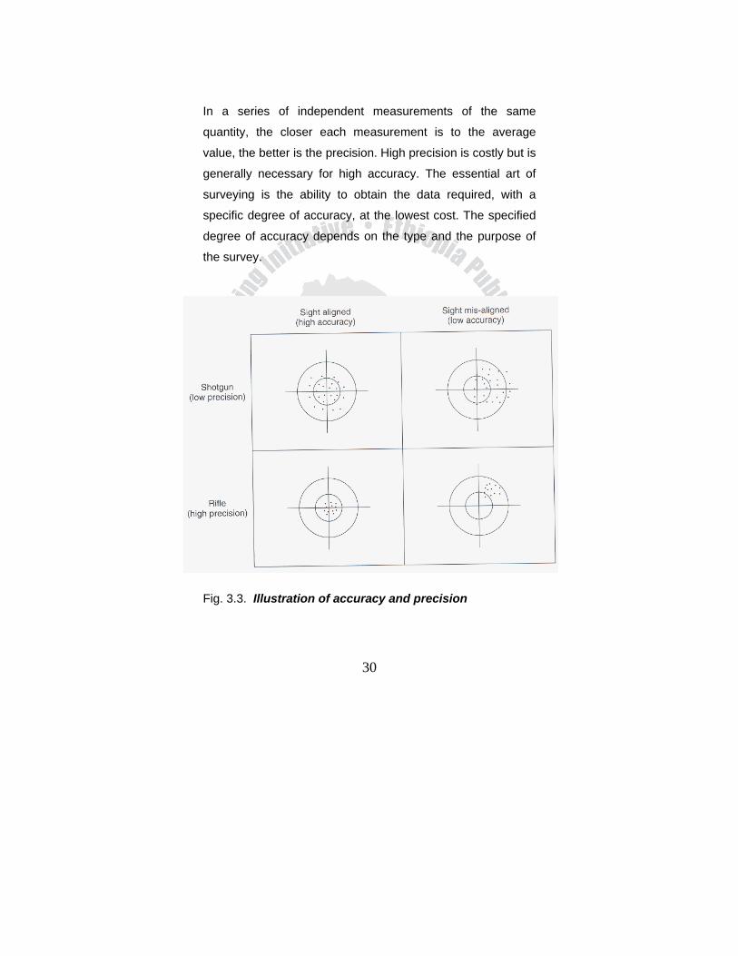
In a series of independent measurements of the same
quantity, the closer each measurement is to the average
value, the better is the precision. High precision is costly but is
generally necessary for high accuracy. The essential art of
surveying is the ability to obtain the data required, with a
specific degree of accuracy, at the lowest cost. The specified
degree of accuracy depends on the type and the purpose of
the survey.
Fig. 3.3. Illustration of accuracy and precision
31
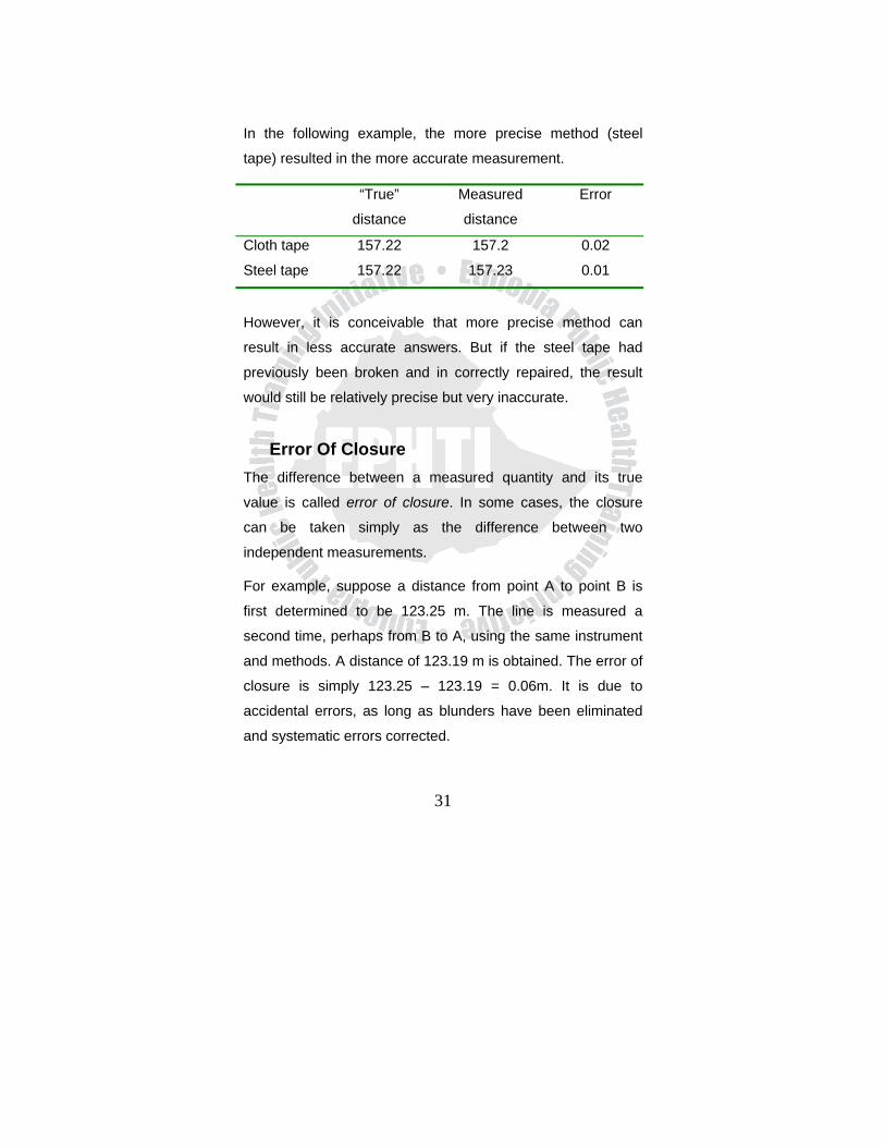
In the following example, the more precise method (steel
tape) resulted in the more accurate measurement.
“True”
distance
Measured
distance
Error
Cloth tape 157.22 157.2 0.02
Steel tape 157.22 157.23 0.01
However, it is conceivable that more precise method can
result in less accurate answers. But if the steel tape had
previously been broken and in correctly repaired, the result
would still be relatively precise but very inaccurate.
Error Of Closure The difference between a measured quantity and its true
value is called error of closure. In some cases, the closure
can be taken simply as the difference between two
independent measurements.
For example, suppose a distance from point A to point B is
first determined to be 123.25 m. The line is measured a
second time, perhaps from B to A, using the same instrument
and methods. A distance of 123.19 m is obtained. The error of
closure is simply 123.25 – 123.19 = 0.06m. It is due to
accidental errors, as long as blunders have been eliminated
and systematic errors corrected.
32
Relative Accuracy For horizontal distances, the ratio of the error of closure to the
actual distance is called the relative accuracy. Relative
accuracy is generally expressed as a ratio with unity as the
first number of numerator. For example, if a distance of 500 ft
were measured with a closure of 0.25 ft, we can say that the
relative accuracy of that particular survey is 0.25/500, or
1/2000. This is also written as 1:2000. This means basically
that for every 2000 ft measured, there is an error of 1 ft. The
relative accuracy of a survey can be compared with a
specified allowable standard of accuracy in order to determine
whether the results of the survey are acceptable.
Relative accuracy can be computed from the following
formula:
Where D = distance measured.
C = error of closure.
Relative accuracy = 1: D/C
33
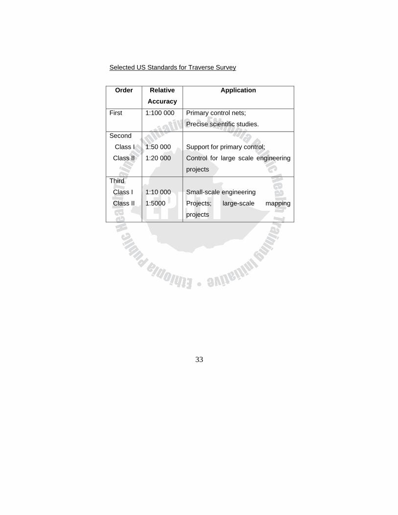
Selected US Standards for Traverse Survey
Order Relative Accuracy
Application
First 1:100 000 Primary control nets;
Precise scientific studies.
Second
Class I
Class II
1:50 000
1:20 000
Support for primary control;
Control for large scale engineering
projects
Third
Class I
Class II
1:10 000
1:5000
Small-scale engineering
Projects; large-scale mapping
projects
34
Exercise 1. Define the term blunder and error.
2. Write the difference between blunder and error.
3. What are the basic difference between systematic error
and an accidental error?
4. Indicate the type of error or mistake- the following would
cause as A (Accidental), S (Systematic) or B (Blunder): a. Swinging plumb bob while taping b. Using a repaired tape c. Aiming the theodolite at the wrong point d. Recopying field data e. Reading a 9 to a 6 f. Surveying with a level that is not leveled g. Having too long a sight distance between the
level and the level rod 5. Convert the following angles to decimal degree form:
a. 35020’(use two decimal places)
b. 129035’15”(use four decimal places)
6. Convert the following angles to degree, minutes, and
seconds:
a. 45.750(to the nearest minute)
b. 123.12340(to the nearest second)
7. What is the sum of 45035’45” and 65050’22”? Subtract
45052’35” from 107032’00”.
35
8. Covert the following angles to the sexagesimal system:
a. 75g b. 125.75g c. 200.4575g
9. How many significant digits are in the following numbers?
a. 0.00123 b. 1.00468 c. 245.00
d. 24500 e. 10.01 f. 45.6
g. 1200 h. 1200• i. 54.0
j. 0.0987
10. Round off the sum of 105.4, 43.67, 0.975, and 34.55 to
the appropriate number of decimal places.
11. Express the product of 1.4685 × 3.58 to the proper
number of significant figures.
12. Express the quotient of 34.67 ÷ 0.054 to the proper
significant figures.
13. Round off the following numbers to three significant
figures: 45.036, 245 501, 0.12345, 251.49, 34.009.
14. A distance was taped six times with the following results:
85.87, 86.03, 85.80, 85.95, 86.06, and 85.90 m.
Compute the 90 percent error of the survey.
15. With reference to the above problem, what would the
maximum anticipated error be for a survey that was three
times as long, if the same precision was used?
16. A group of surveying students measure a distance twice,
obtaining 67.455 and 67.350 m. What is the relative
accuracy of the measurements?
36
17. Determine the accuracy of the following, and name the
order of accuracy with reference to the US standards
summarized.
Error, m Distance, m 8.0 30560
0.07 2000
1.32 8460
0.13 1709
1.0 17543
0.72 1800
18. What is the maximum error of closure in a measurement
of 2500 ft if the relative accuracy is 1:5000?
37
CHAPTER FOUR MEASURING HORIZONTAL DISTANCES
4.1. Learning Objectives At the end of this chapter, the student will be able to:
1. Measure horizontal distance
2. Identify and use different measurements
3. Identify equipments of horizontal measurement.
4. Identify the sources of errors and corrective actions.
4.2. Introduction The tasks of determining the horizontal distances between
two existing points and of setting a new point at a specified
distance from some other fixed position are fundamental
surveying operations. The surveyor must select the
appropriate equipment and apply suitable field procedures in
order to determine or set and mark distances with the required
degree of accuracy.
Depending on the specific application and the required
accuracy, one of several methods may be used to determine
horizontal distance. The most common methods include
pacing, stadia, taping, and EDM. Here, we will try to see the
rough distance measurement by pacing and by using a
measuring wheel. Stadia is an indirect method of
38
measurement that makes use of a transit, leveling and
trigonometry.
Taping has been the traditional surveying method for
horizontal distance measurement for many years. It is a direct
and relatively slow procedure, which requires manual skill on
the part of the surveyors.
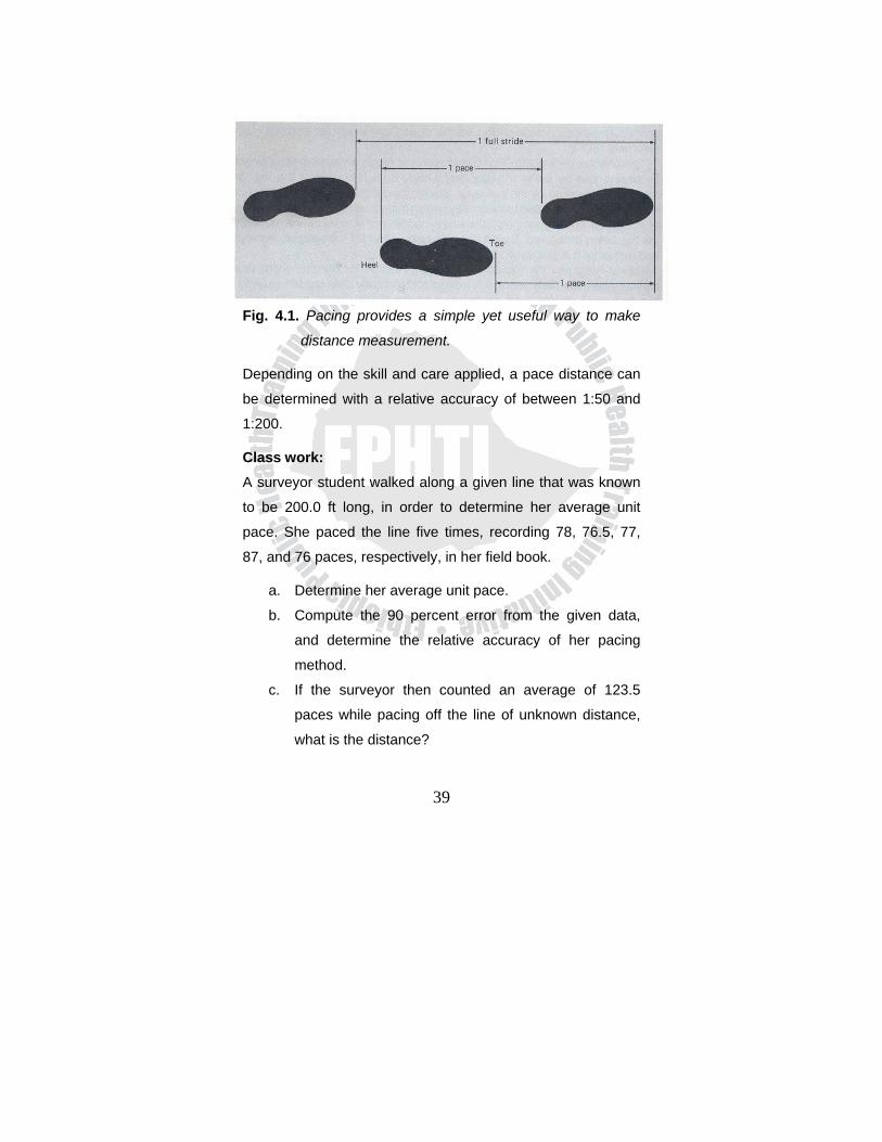
4.3. Rough Distance Measurement In certain surveying applications, only a rough approximation
of distance is necessary; a method called pacing, or the use
of a simple measuring wheels, may be sufficient in these
instances , e.g. locating topographic features during the
preliminary reconnaissance of a building site, searching
for the property corners etc. In this method, distances can be
measured with an accuracy of about 1:100 by pacing. While
providing only a crude measurement of distances, pacing has
the significance advantage of requiring no equipment. It is a
skill every surveyor should have. Pacing simply involves
counting steps or paces while walking naturally along the line
to be measured.
Distance = Unit Pace × Number of Paces
39
Fig. 4.1. Pacing provides a simple yet useful way to make
distance measurement.
Depending on the skill and care applied, a pace distance can
be determined with a relative accuracy of between 1:50 and
1:200.
Class work: A surveyor student walked along a given line that was known
to be 200.0 ft long, in order to determine her average unit
pace. She paced the line five times, recording 78, 76.5, 77,
87, and 76 paces, respectively, in her field book.
a. Determine her average unit pace.
b. Compute the 90 percent error from the given data,
and determine the relative accuracy of her pacing
method.
c. If the surveyor then counted an average of 123.5
paces while pacing off the line of unknown distance,
what is the distance?

40
USING THE MEASURING WHEEL
A simple measuring wheel mounted on a rod can be used to
determine distances, by pushing the rod and rolling the wheel
along the line to be measured. An attached device called an
odometer serves to count the number of turns of the wheels.
From the known circumference of the wheel and the number
of revolutions, distances for reconnaissance can be
determined with relative accuracy of about 1:200. This device
is particularly useful for rough measurement of distance along
curved lines.
Fig. 4.2. A typical measuring wheel used for making rough
distance measurements.
41
Where D is the diameter of the measuring wheel
4.4. Taping Equipments and Methods Measuring horizontal distances with a tape is simple in theory,
but in actual practice, it is not as easy as it appears at first
glance. It takes skill and experience for a surveyor to be able
to tape a distance with a relative accuracy between 1:3000
and 1:5000, which is generally acceptable range for most
preliminary surveys.
4.4.1. Tapes and Accessories
Most of the original surveys were done using Gunter’s chain
for measurement of horizontal distances. To this day, the term
chaining is frequently used to describe the taping operation.
While the Gunter’s chain itself is no longer actually used, steel
tapes graduated in units of chains and links are still available.
Steel Tapes
Modern steel tapes are available in variety of lengths and
cross sections; among the most commonly used are the 100ft-
tape and the 30-m tape, which are ¼ in and 6 mm wide,
respectively. Both lighter as well as heavier duty tapes are
also available.
Distance= Odometer Reading X Circumference of the Wheel (ΠD)
42
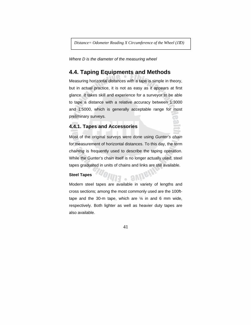
Fig. 4.3. Fiberglass tapes (a) Closed case; (b) Open reel
4.4.2. Accessories for Taping Accurate taping cannot be done with the tape alone. When
taping horizontal distances, the tape very often must be held
above the ground at one or both ends. One of the most
important accessories for proper horizontal taping is the
plumb bob. It is a small metal weight with a sharp, replaceable
point. Freely suspended from a chord, the plumb bob is used
to project the horizontal position of a point on the ground up to
the tape, or vice versa.
43
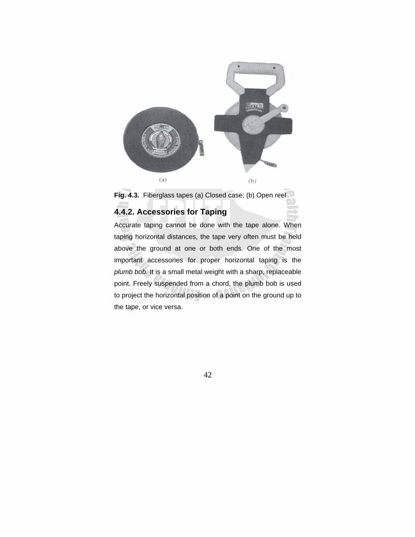
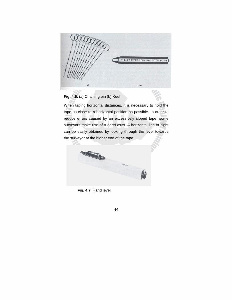
Fig. 4.4. A plumb bob: (is one of the simplest yet most
important accessories for accurate surveying.)
Fig. 4.5. A surveyor’s range pole.
When a transit or theodolite is not used to establish direction,
range pole serve to establish a line of sight and keep the
surveyors properly aligned. A range pole would be placed
vertically in the ground behind each endpoint of the line to be
measured.
Steel taping pins are used for marking the end of the tape, or
intermediate points, when taping over grass or unpaved
ground. Taping pins are most useful for tallying full tape
lengths over long measured distances.
44
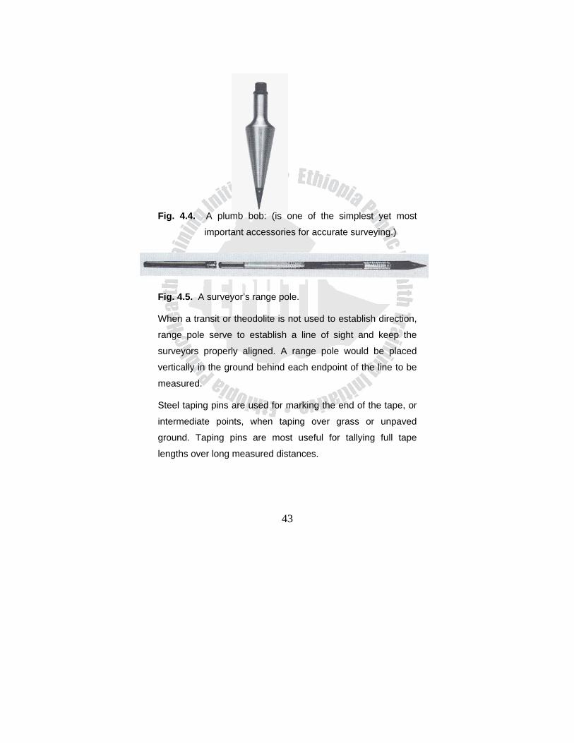
Fig. 4.6. (a) Chaining pin (b) Keel
When taping horizontal distances, it is necessary to hold the
tape as close to a horizontal position as possible. In order to
reduce errors caused by an excessively sloped tape, some
surveyors make use of a hand level. A horizontal line of sight
can be easily obtained by looking through the level towards
the surveyor at the higher end of the tape.
Fig. 4.7. Hand level
45
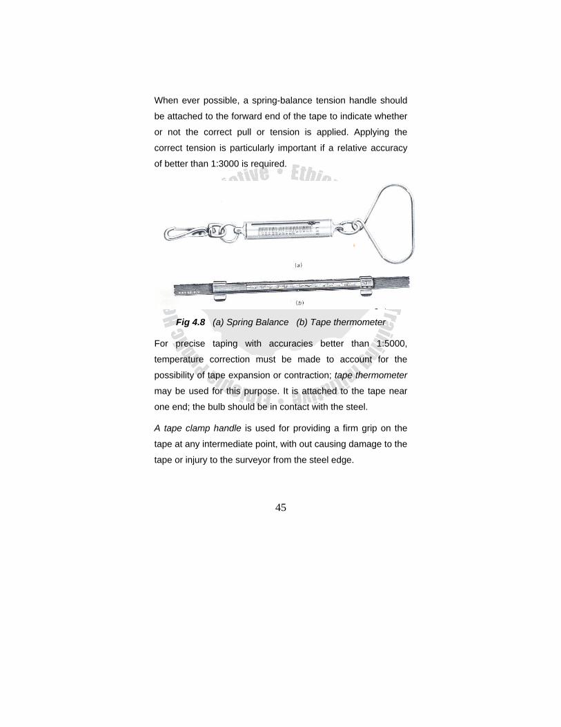
When ever possible, a spring-balance tension handle should
be attached to the forward end of the tape to indicate whether
or not the correct pull or tension is applied. Applying the
correct tension is particularly important if a relative accuracy
of better than 1:3000 is required.
Fig 4.8 (a) Spring Balance (b) Tape thermometer
For precise taping with accuracies better than 1:5000,
temperature correction must be made to account for the
possibility of tape expansion or contraction; tape thermometer
may be used for this purpose. It is attached to the tape near
one end; the bulb should be in contact with the steel.
A tape clamp handle is used for providing a firm grip on the
tape at any intermediate point, with out causing damage to the
tape or injury to the surveyor from the steel edge.
46
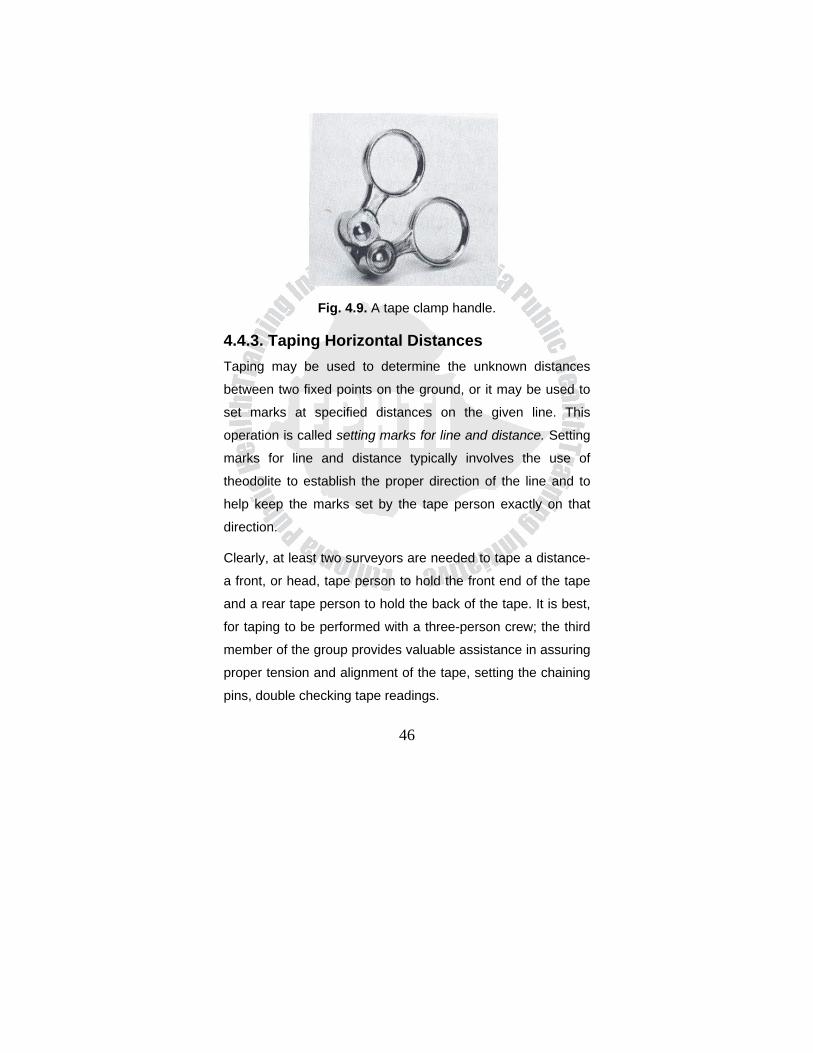
Fig. 4.9. A tape clamp handle.
4.4.3. Taping Horizontal Distances Taping may be used to determine the unknown distances
between two fixed points on the ground, or it may be used to
set marks at specified distances on the given line. This
operation is called setting marks for line and distance. Setting
marks for line and distance typically involves the use of
theodolite to establish the proper direction of the line and to
help keep the marks set by the tape person exactly on that
direction.
Clearly, at least two surveyors are needed to tape a distance-
a front, or head, tape person to hold the front end of the tape
and a rear tape person to hold the back of the tape. It is best,
for taping to be performed with a three-person crew; the third
member of the group provides valuable assistance in assuring
proper tension and alignment of the tape, setting the chaining
pins, double checking tape readings.
47
When a series of marks are set on a line at measured
distances, surveyor uses a standard system of identifying the
marks; the marks are called stations. The stations may be
very temporary or somewhat long lasting. Stationing is
particularly important when doing profile leveling, as well as
when setting marks for line and distance in route survey.
4.4.4. Horizontal Measurement on Sloping Ground and slop measurements
In taping on uneven or sloping ground, it is standard practice
to hold the tape horizontal and use a plumb bob at one or
both ends. It is difficult to keep the plumb line steady for
height above the chest. Wind exaggerates the problem and
may make accurate work impossible.
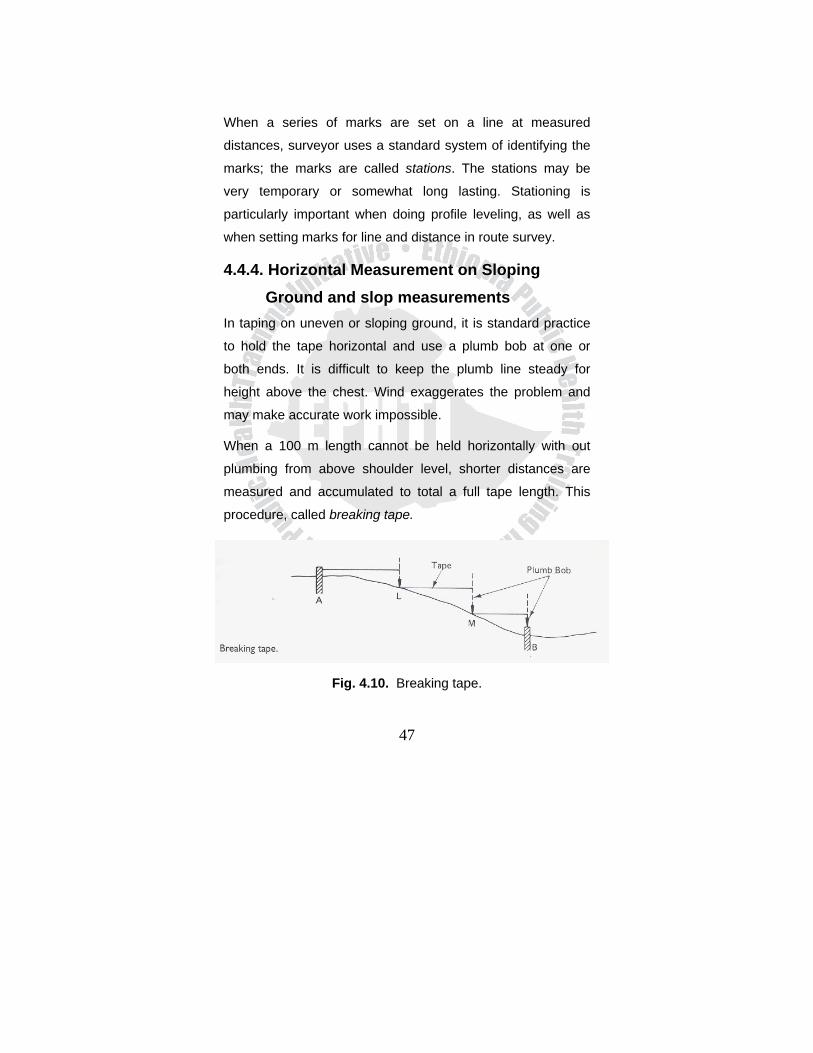
When a 100 m length cannot be held horizontally with out
plumbing from above shoulder level, shorter distances are
measured and accumulated to total a full tape length. This
procedure, called breaking tape.
Fig. 4.10. Breaking tape.
48
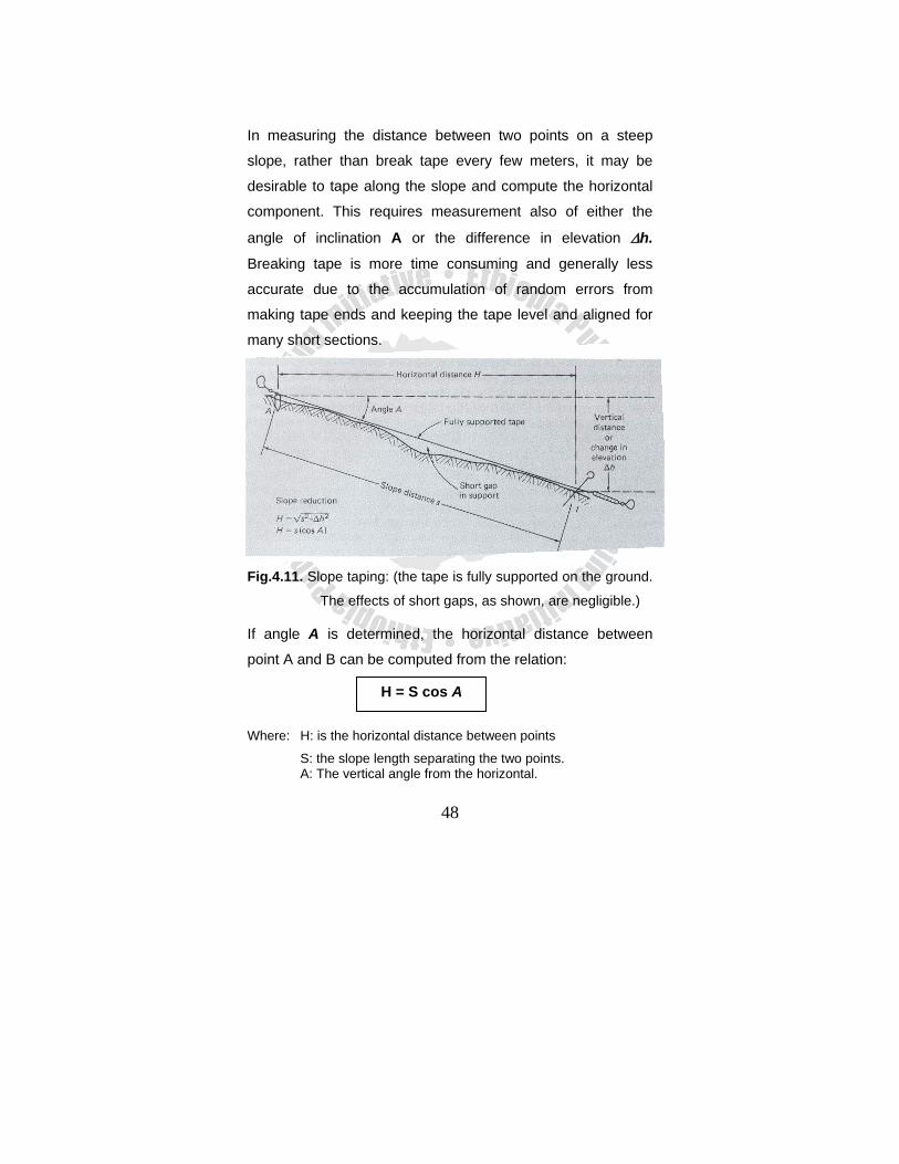
In measuring the distance between two points on a steep
slope, rather than break tape every few meters, it may be
desirable to tape along the slope and compute the horizontal
component. This requires measurement also of either the
angle of inclination A or the difference in elevation Δh.
Breaking tape is more time consuming and generally less
accurate due to the accumulation of random errors from
making tape ends and keeping the tape level and aligned for
many short sections.
Fig.4.11. Slope taping: (the tape is fully supported on the ground.
The effects of short gaps, as shown, are negligible.)
If angle A is determined, the horizontal distance between
point A and B can be computed from the relation:
Where: H: is the horizontal distance between points
S: the slope length separating the two points. A: The vertical angle from the horizontal.
H = S cos A
49
If the difference in elevation’d’ between the ends of the tape is
measured, which is done by leveling, the horizontal distance
can be computed using the following expression
Another approximate formula may be used to reduce slope
distance to horizontal.
4.4.5. Identifying Stations A zero position is usually established at the beginning of the
survey or at the beginning of the line to be marked out. This
zero point is identified as 0+00. Each point located at the
intervals of exactly 100 m from the beginning point is called a
full station and is identified as follows: a point 100 m from
0+00 is labeled station 1+00, a point 200 m from the zero
point is station 2+00, and so on.
Points located between the full stations are identified as
follows: a point 350 m from the zero point is called 3+50, and
a point 475 m from zero is called 4+75. At a distance of
462.78 m from the zero, the station called 4+62.78. The +50,
+75, +62.78 are called pluses.
H = √(s2-Δh2)
H = S - Δh2/2S

50
Fig. 4.12. The positions along a measured line are called
stations.
4.4.6. Taping Mistakes and Errors As in any kind of surveying operation, taping blunders must be
eliminated, and tapping errors, both random and systematic,
must be minimized to achieve accurate results.
Example of TAPING MISTAKES AND BLUNDERS:
Misreading the tape, particularly reading a 6 for a 9.
Misrecording the reading, particularly by transposing
digits.
51
Mistaking the end point of the tape.
Miscounting full tape length, particularly when long
distances are taped.
Mistaking station markers.
Sources of Errors in Taping There are three fundamental sources of errors in taping.
1. Instrumental errors: A tape may differ in actual length
from its nominal graduation and length because of defects
in manufacturing or repair.
2. Nominal errors: The horizontal distance between end
graduations of a tape varies because of the effects of
temperature, wind and weight of the tape itself.
3. Personal errors: Tape persons may be careless in setting
pins, reading tapes, or manipulating the equipment.
Systematic Errors in Taping Systematic errors in taping linear distances are those
attributable to the following causes
• The tape is not of standard length
• The tape is not horizontal
• Variation in temperature
• Variation in tension
• Sag
• Incorrect alignment of tape
• The tape is not straight
52
4.4.7. Corrections 1. Incorrect Length of Tape
Incorrect length of a tape can be one of the most important
errors. It is systematic.
For example, a 100 m steel tape usually is standardized under
set of condition- 680F and 12 lb pull.
An error due to incorrect length of a tape occurs each time the
tape is used. If the true length, known by standardization, is
not exactly equal to its nominal value of 100.00 m recorded for
every full length, the correction can be determined and
applied from the formulas:
Where: Cl: is the correction to be applied to the measured length of a line to obtain the true length
l: the actual tape length l’: the nominal tape length L: the measured length of the line
L : The corrected length of the line.
Sometimes, the changes in length are quite small and of little
importance in many types of surveys. However, when good
relative accuracy is required, the actual tape length must be
known within 0.005 ft (1.5 mm). The actual length of a working
tape, then, must be compared with a standard tape
L = L + Cl Ll
llCl ⎟⎟⎠
⎞⎜⎜⎝
⎛ −=
'
'
53
periodically. When its actual length is known, the tape is said
to be standardized. A correction must be added or subtracted
to a measured distance whenever its standardized length
differs from its nominal or graduated length.
N.B: In measuring unknown distances with a tape that is too
long, a correction must be added. Conversely, if the tape
is too short, the correction will be minus, resulting in
decrease.
2. Temperature Other Than Standards
Steel tapes are standardized for 680F or 200C. A temperature
higher than or lower than this value causes a change in length
that must be considered. The coefficient of thermal expansion
and contraction of steel used in ordinary tapes is
approximately 1.16 x 10⁻⁵ per length per 0C. For any tapes the
correction for temperature can be computed and applied using
the formula
Where: Ct: is the correction in length of a line due to nonstandard temperature.
K: the coefficient of thermal expansion and correction of the tape. T1: the tape temperature at the time of measurement. T: the tape temperature when it has standard length. L: the measured lengthy of the line.
L : The corrected length of the line.
Ct = K (T1 - T) L L = L + Ct
54
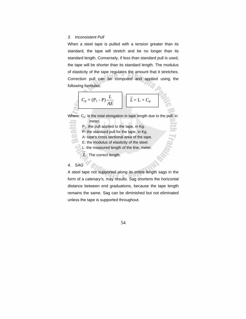
3. Inconsistent Pull
When a steel tape is pulled with a tension greater than its
standard, the tape will stretch and be no longer than its
standard length. Conversely, if less than standard pull is used,
the tape will be shorter than its standard length. The modulus
of elasticity of the tape regulates the amount that it stretches.
Correction pull can be computed and applied using the
following formulas:
Where: Cp: is the total elongation in tape length due to the pull, in meter.
P1: the pull applied to the tape, in Kg. P: the standard pull for the tape, in Kg. A: tape's cross sectional area of the tape. E: the modulus of elasticity of the steel. L: the measured length of the line, meter.
L : The correct length.
4. SAG
A steel tape not supported along its entire length sags in the
form of a catenary's, may results. Sag shortens the horizontal
distance between end graduations, because the tape length
remains the same. Sag can be diminished but not eliminated
unless the tape is supported throughout.
L = L + Cp Cp = (P1 - P)AEL

55
The following formulas are used to compute the sag
correction:
OR
Where Cs: is the correction for sag, in meter.
Ls: the unsupported length of the tape, in meter.
w: weight of the tape per meter of length.
W: total weight of the tape between the supports, Kg.
P1: is the pull on the tape, in Kg.
In measuring lines of unknown length, the sag correction is
always negative. After a line has been measured in several
segments, and a sag correction has been calculated for each
segment, the corrected length is given by
Where L : is the corrected length of the line.
L: the recorded length of the line
∑Cs: the sum of individual sag corrections.
5. Normal Tension
By equating equations CS = CP,
Cs = 21
2
24PLW s Cs = 2
1
32
24PLw s
L = L + ∑Cs
w 2Ls3 = (P1-P) L
24P12 AE
56
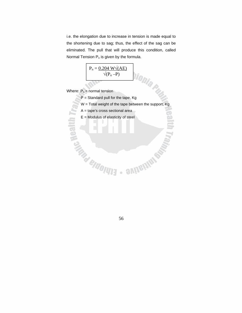
i.e. the elongation due to increase in tension is made equal to
the shortening due to sag; thus, the effect of the sag can be
eliminated. The pull that will produce this condition, called
Normal Tension Pn is given by the formula.
Where: Pn = normal tension
P = Standard pull for the tape, Kg
W = Total weight of the tape between the support, Kg
A = tape’s cross sectional area
E = Modulus of elasticity of steel
Pn = 0.204 W√(AE) √(Pn –P)
57
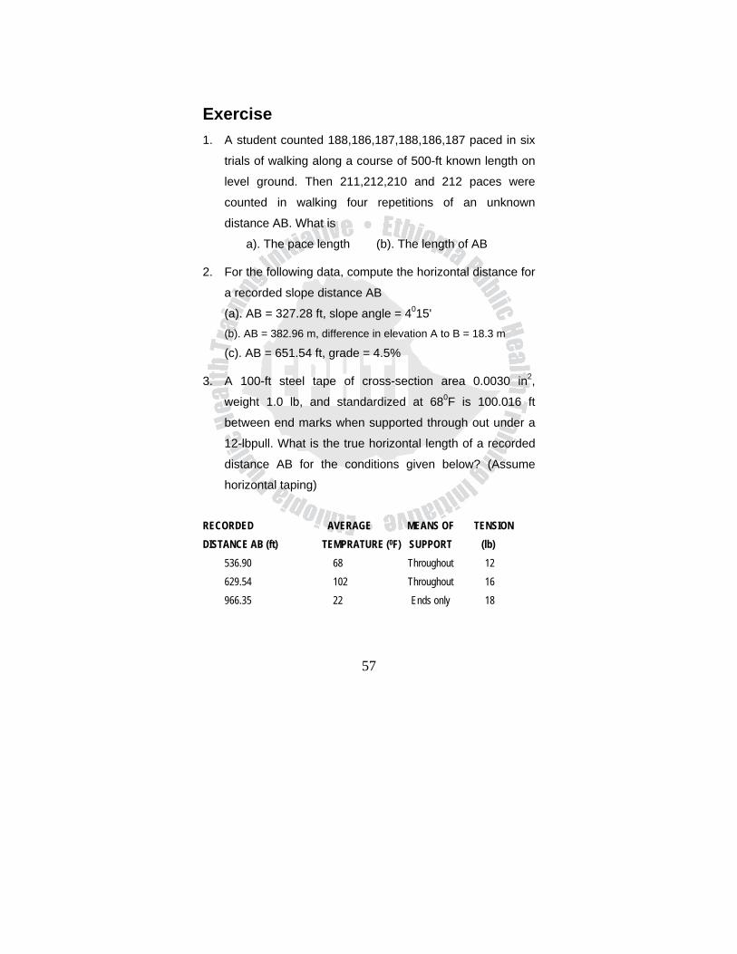
Exercise 1. A student counted 188,186,187,188,186,187 paced in six
trials of walking along a course of 500-ft known length on
level ground. Then 211,212,210 and 212 paces were
counted in walking four repetitions of an unknown
distance AB. What is
a). The pace length (b). The length of AB
2. For the following data, compute the horizontal distance for
a recorded slope distance AB
(a). AB = 327.28 ft, slope angle = 4015' (b). AB = 382.96 m, difference in elevation A to B = 18.3 m
(c). AB = 651.54 ft, grade = 4.5%
3. A 100-ft steel tape of cross-section area 0.0030 in2,
weight 1.0 lb, and standardized at 680F is 100.016 ft
between end marks when supported through out under a
12-lbpull. What is the true horizontal length of a recorded
distance AB for the conditions given below? (Assume
horizontal taping)
RECORDED AVERAGE MEANS OF TENSION DISTANCE AB (ft) TEMPRATURE (0F) SUPPORT (lb)
536.90 68 Throughout 12 629.54 102 Throughout 16 966.35 22 Ends only 18
58
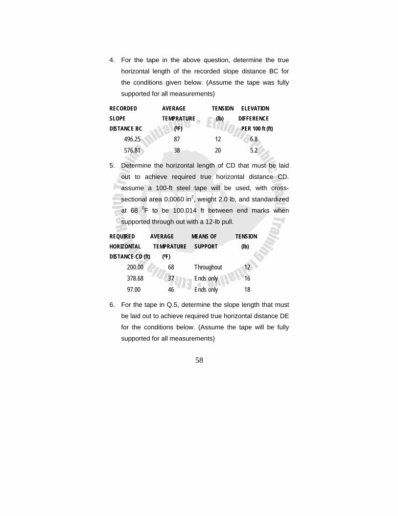
4. For the tape in the above question, determine the true
horizontal length of the recorded slope distance BC for
the conditions given below. (Assume the tape was fully
supported for all measurements)
RECORDED AVERAGE TENSION ELEVATION SLOPE TEMPRATURE (lb) DIFFERENCE DISTANCE BC (0F) PER 100 ft (ft)
496.25 87 12 6.8 576.81 38 20 5.2
5. Determine the horizontal length of CD that must be laid
out to achieve required true horizontal distance CD.
assume a 100-ft steel tape will be used, with cross-
sectional area 0.0060 in2, weight 2.0 lb, and standardized
at 68 0F to be 100.014 ft between end marks when
supported through out with a 12-lb pull.
REQUIRED AVERAGE MEANS OF TENSION HORIZONTAL TEMPRATURE SUPPORT (lb) DISTANCE CD (ft) (0F)
200.00 68 Throughout 12 378.68 37 Ends only 16 97.00 46 Ends only 18
6. For the tape in Q.5, determine the slope length that must
be laid out to achieve required true horizontal distance DE
for the conditions below. (Assume the tape will be fully
supported for all measurements)
59
REQUIRED AVERAGE TENSION SLOPE HORIZONTAL TEMPRATURE (lb) DISTANCE DE (ft) (0F)
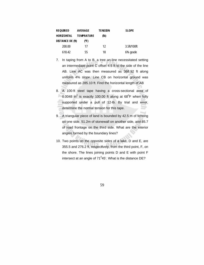
200.00 17 12 3.5ft/100ft 618.42 55 18 6% grade
7. In taping from A to B, a tree on-line necessitated setting
an intermediate point C offset 4.5 ft to the side of the line
AB. Line AC was then measured as 368.92 ft along
uniform 4% slope. Line CB on horizontal ground was
measured as 285.10 ft. Find the horizontal length of AB
8. A 100-ft steel tape having a cross-sectional area of
0.0048 in2 is exactly 100.00 ft along at 680F when fully
supported under a pull of 12-lb. By trial and error,
determine the normal tension for this tape.
9. A triangular piece of land is bounded by 42.5 m of fencing
on one side, 51.2m of stonewall on another side, and 85.7
of road frontage on the third side. What are the interior
angles formed by the boundary lines?
10. Two points on the opposite sides of a lake, D and E, are
355.5 and 276.2 ft, respectively, from the third point, F, on
the shore. The lines joining points D and E with point F
intersect at an angle of 71045’. What is the distance DE?
60
CHAPTER FIVE LEVELING
5.1. LEARNING OBJECTIVES At the end of this chapter, the students will be able to:
1. Define and describe different types of leveling.
2. Understand the principles of leveling and measure
vertical distances
3. Apply the skills of leveling
4. Identify measurement errors and take corrective
actions.
5.2 Introduction Leveling is the general term applied to any of the various
processes by which elevations of points or differences in
elevation are determined. It is a vital operation in producing
necessary data for mapping, engineering design, and
construction.
Leveling results are used to:
1. Design highways, railroads, canals, sewers etc.
2. Layout construction projects according to planned
elevations.
3. Calculate volume of earthwork and other materials.
4. Investigate drainage characteristics of the area.
5. Develop maps showing ground configuration.
61
5.3. Measuring Vertical Distances The vertical direction is parallel to the direction of gravity; at
any point, it is the direction of a freely suspended plumb-bob
cord. The vertical distance of a point above or below a given
reference surface is called the elevation of the point. The most
commonly used reference surface for vertical distance is
mean sea level. The vertical distances are measured by the
surveyor in order to determine the elevation of points, in a
process called running levels or leveling.
The determination and control of elevations constitute a
fundamental operation in surveying and engineering projects.
Leveling provides data for determining the shape of the
ground and drawing topographic maps and the elevation of
new facilities such as roads, structural foundations, and
pipelines.
5.4. Methods OF Leveling There are several methods for measuring vertical distances
and determining the elevations of points. Traditional methods
include barometric leveling, trigonometric leveling and
differential leveling. Two very advanced and sophisticated
techniques include inertia leveling and global positioning
systems.
62
1. Barometric leveling By using special barometers to measure air pressure (which
decrease with increasing elevation), the elevation of points on
the earth's surface can be determined within ±1m. This
method is useful for doing a reconnaissance survey of large
areas in rough country and for obtaining preliminary
topographic data.
2. Differential leveling By far the most common leveling method, and the one which
most surveyors are concerned with, is differential leveling. It
may also be called spirit leveling, because the basic
instrument used comprises a telescopic sight and a sensitive
spirit bubble vial. The spirit bubble vial serves to align the
telescopic sight in a horizontal direction, that is, perpendicular
to the direction of gravity.
Briefly, a horizontal line of sight is first established with an
instrument called a level. The level is securely mounted on a
stand called a tripod, and the line of sight is made horizontal.
Then the surveyor looks through the telescopic sight towards
a graduated level rod, which is held vertically at a specific
location or point on the ground. A reading is observed on the
rod where it appears to be intercepted by the horizontal cross
hair of the level; this is the vertical distance from the point on
the ground up to the line of sight of the instrument.
63
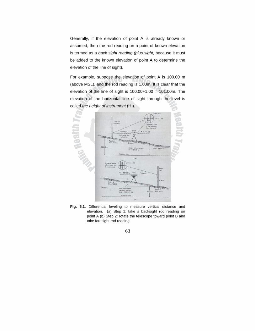
Generally, if the elevation of point A is already known or
assumed, then the rod reading on a point of known elevation
is termed as a back sight reading (plus sight, because it must
be added to the known elevation of point A to determine the
elevation of the line of sight).
For example, suppose the elevation of point A is 100.00 m
(above MSL), and the rod reading is 1.00m. It is clear that the
elevation of the line of sight is 100.00+1.00 = 101.00m. The
elevation of the horizontal line of sight through the level is
called the height of instrument (HI).
Fig. 5.1. Differential leveling to measure vertical distance and
elevation. (a) Step 1: take a backsight rod reading on point A (b) Step 2: rotate the telescope toward point B and take foresight rod reading.
64
Suppose we must determine the elevation of point B. The
instrument person turns the telescope so that it faces point B,
and reads the rod now held vertically on that point. For
example, the rod reading might be 4.00m. A rod reading on a
point of unknown elevation is called foresight (minus sight).
Since the HI was not changed by turning the level, we can
simply subtract the foresight reading of 4.00 from the HI of
101.00 to obtain the elevation of point B, resulting here in
101.00 - 4.00 = 97.00m.
The operation of reading a vertical rod held alternately on two
nearby points is the essence of differential leveling. The
difference between the two rod readings is, in effect, the
vertical distance between the two points.
The basic cycle of differential leveling can be summarized as
follows:
Frequently, the elevations of points over a relatively long
distance must be determined. A process of measuring two or
more widely separated points simply involves several cycles
or repetitions of the basic differential leveling operation. More
Height of Instrument = Known elevation + backsight HI = ElevA + BS
New elevation = height of instrument – foresight ElevB = HI - FS
65
specific terms for this are benchmark, profile, and topographic
leveling.
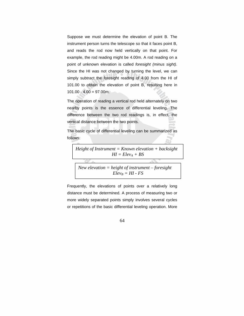
5.5 Benchmarks and Turning Points Suppose it is necessary to determine the elevation of some
point C from point A. But in this case, let us assume that it is
not possible to set up the level so that both points A and C are
visible from one position. The line of levels can be carried
forward towards C by establishing a convenient and
temporary turning point (TP) somewhere between A and C.
The selected TP serves merely as an intermediate reference
point; it does not have to be actually set in the ground as a
permanent monument.
Fig. 5.2. Temporary turning points are used to carry a line of levels from a benchmark to some other station or benchmark; the process of differential leveling is repeated at each instrument set up.
66
The elevation of the turning point is computed from the first
pair of BS and FS readings. The BS is on point A, which is the
end point of known elevation. A secure and permanent point
of known elevation is called a bench mark (BM); a leveling
survey should begin with a back sight on a benchmark. The
BS is added to the elevation to give the HI at the first
instrument position.
The elevation of the turning point is obtained by subtracting
the FS from the HI. Once the elevation of the turning point is
known, the level instrument can be moved to another location,
one closer to C but still in sight of the turning point. Then
another back sight is taken, this time on the turning point, in
order to determine the new height of instrument. Finally a
foresight is taken on point C, and its elevation is computed.
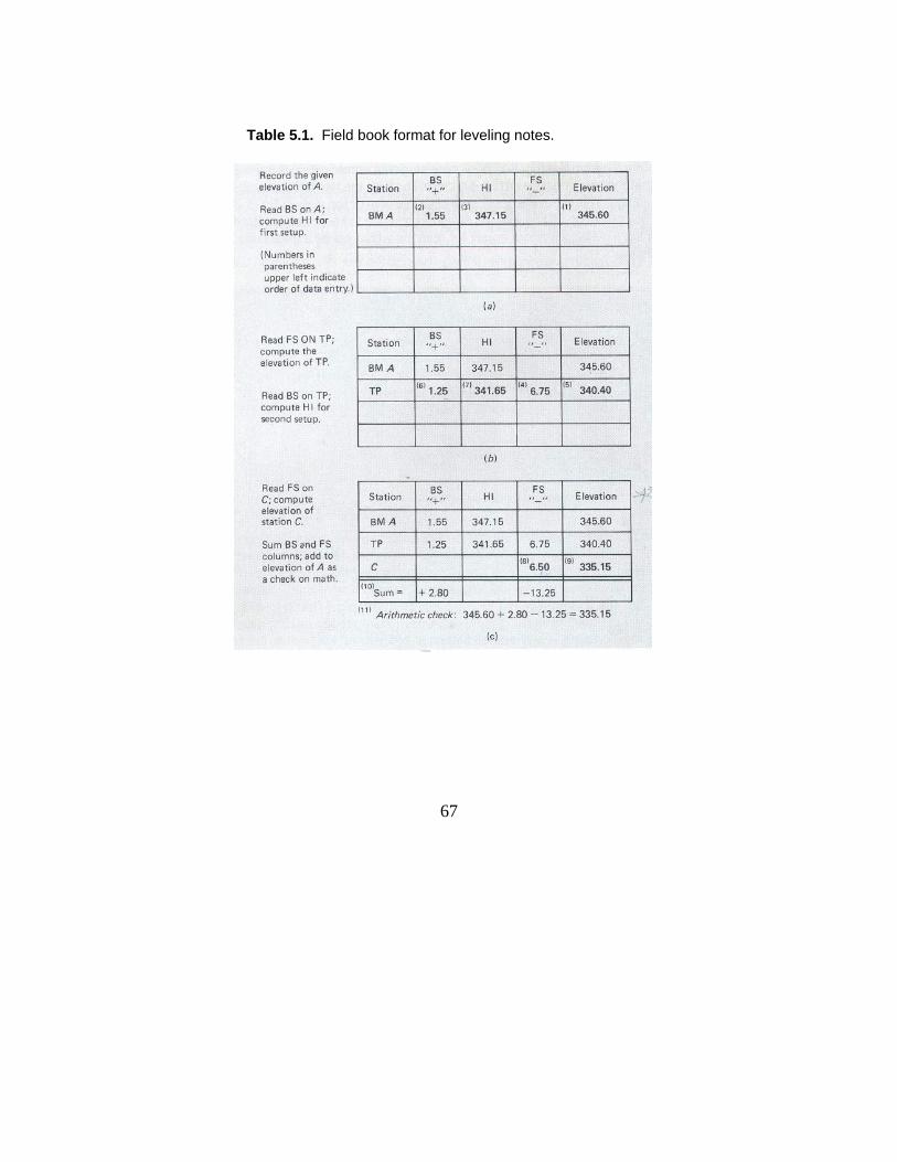
67
Table 5.1. Field book format for leveling notes.
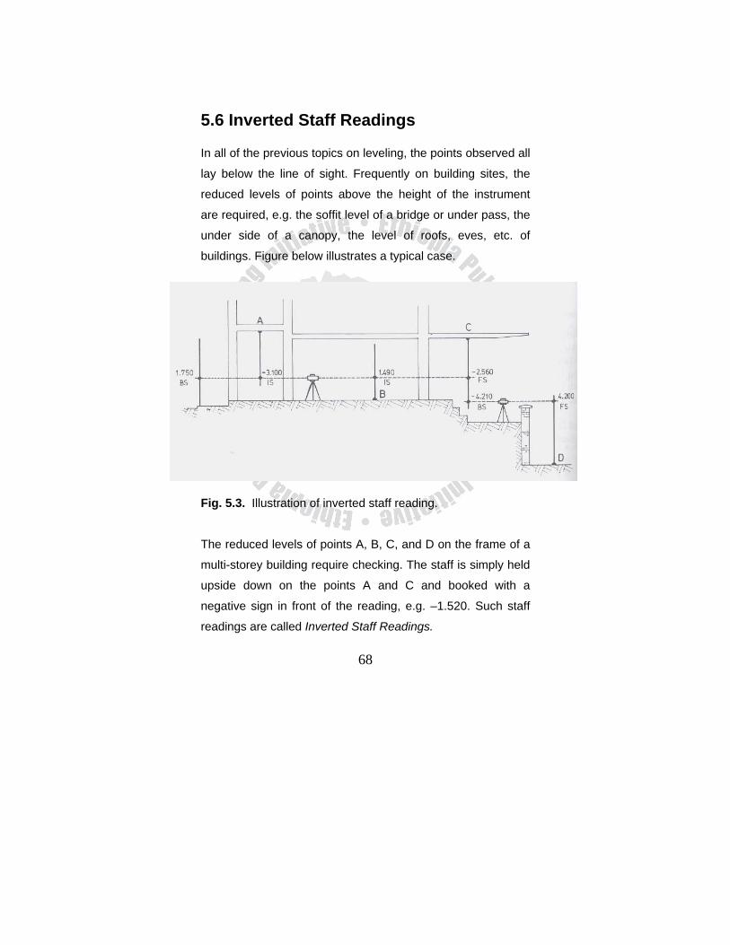
68
5.6 Inverted Staff Readings
In all of the previous topics on leveling, the points observed all
lay below the line of sight. Frequently on building sites, the
reduced levels of points above the height of the instrument
are required, e.g. the soffit level of a bridge or under pass, the
under side of a canopy, the level of roofs, eves, etc. of
buildings. Figure below illustrates a typical case.
Fig. 5.3. Illustration of inverted staff reading.
The reduced levels of points A, B, C, and D on the frame of a
multi-storey building require checking. The staff is simply held
upside down on the points A and C and booked with a
negative sign in front of the reading, e.g. –1.520. Such staff
readings are called Inverted Staff Readings.
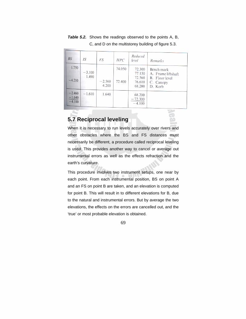
69
Table 5.2. Shows the readings observed to the points A, B,
C, and D on the multistorey building of figure 5.3.
5.7 Reciprocal leveling When it is necessary to run levels accurately over rivers and
other obstacles where the BS and FS distances must
necessarily be different, a procedure called reciprocal leveling
is used. This provides another way to cancel or average out
instrumental errors as well as the effects refraction and the
earth’s curvature.
This procedure involves two instrument setups, one near by
each point. From each instrumental position, BS on point A
and an FS on point B are taken, and an elevation is computed
for point B. This will result in to different elevations for B, due
to the natural and instrumental errors. But by average the two
elevations, the effects on the errors are cancelled out, and the
‘true’ or most probable elevation is obtained.
70
5.8 Leveling Equipment There are several types of surveying levels and level rods.
Some are meant primarily for precise leveling work, and
others are much better suited for ordinary construction and
operation of the various types of leveling equipments, so as to
be able to select and use the best instrument for a particular
surveying assignment.
Compared with a transit or theodolite, the level is a relatively
simple instrument. It is only required to give a horizontal line
of sight in all directions of the compass, and this is easily
accomplished using basic optical and mechanical
components.
A surveying level basically consists of a telescope and a
sensitive spirit bubble vial. The spirit level vial can be adjusted
so that, when the bubble is centered, the line of sight through
the telescope is horizontal. The telescope is mounted on a
vertical spindle, which fits into a bearing in the leveling head.
The leveling head may have either three, or two leveling
screws, depending on the type of instrument.
The most common types of levels are the dumpy level, the
tilting level and the automatic level. A transit or theodolite may
also be used for leveling work, although the accuracy
obtained is generally less. A simple hand level may be used
for determining the elevations when a high degree of accuracy
is not required.
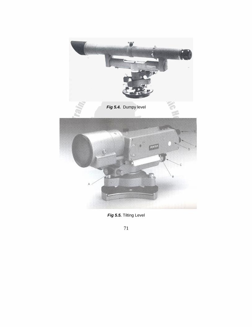
71
Fig 5.4. Dumpy level
Fig 5.5. Tilting Level
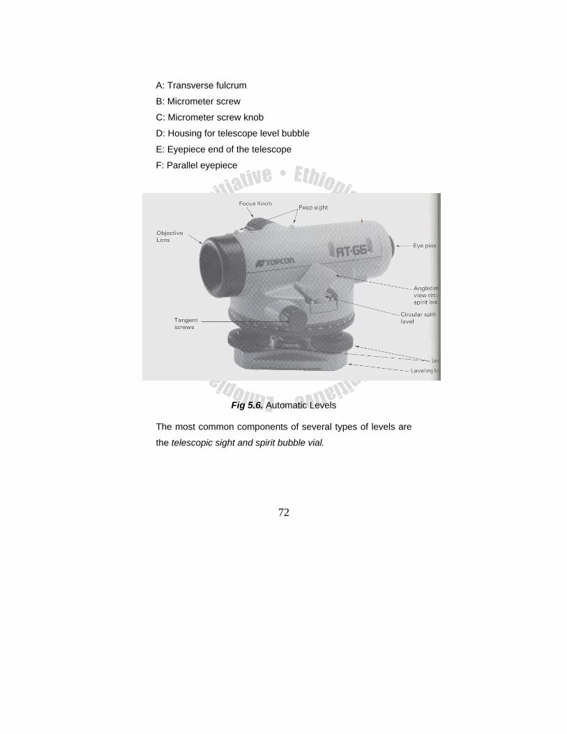
72
A: Transverse fulcrum
B: Micrometer screw
C: Micrometer screw knob
D: Housing for telescope level bubble
E: Eyepiece end of the telescope
F: Parallel eyepiece
Fig 5.6. Automatic Levels
The most common components of several types of levels are
the telescopic sight and spirit bubble vial.
73
a. The Telescopic Sight The modern telescopic sight consists of the following
components:
1. A reticule, which provides the cross hair, near the rear
of the telescope tube.
2. A microscope or eyepiece which magnifies the cross
hair, and which must be focused on them according to
the eyesight of the observer.
3. An objective lens at the forward end of the telescope,
which forms an image of the sight target within the
telescope tube.
4. A focusing lens, which can be moved back and forth
inside the scope to focus the image on the cross hair.
Focusing a Telescoping sight: Three steps are required to focus a telescopic sight for
greatest accuracy.
1. Aim the telescope at the bright, unmarked object,
such as the sky, and regulate the eyepiece until the
cross hair is in sharp focus.
2. Aim the telescope at the object to be viewed and,
while keeping the eye focused on the cross hairs,
regulate the focusing lens until the object is clear.
3. Eliminate parallex.
74
The Line Of Sight A straight line from any point on the image through the optical
center of the objective lens will strike a corresponding point on
the object. A straight line from the cross hairs through the
optical center of the lens will strike the point on the object
where the observer sees the cross hairs apparently located.
Thus the cross hairs and the optical center of the objective
define the line of sight of a telescopic sight.
b. The Spirit Bubble Tube Or Circle A spirit bubble vial consists of a glass container, which is
partly filled with a clear, nonfreezing, very low viscosity liquid
such as alcohol or ether.
Level Rods
There are many different types of level rods. Generally, the
body of the rod is made of seasoned hardwood; this act as a
rigid support for the rod face, a strip of steel graduated
upward starting from zero at the bottom. The rod person, on a
point of known elevation for a BS, or a point of unknown
elevation, holds the rod vertically for an FS. The rod is then
observed with the level and read by the instrument person on
the target rod.
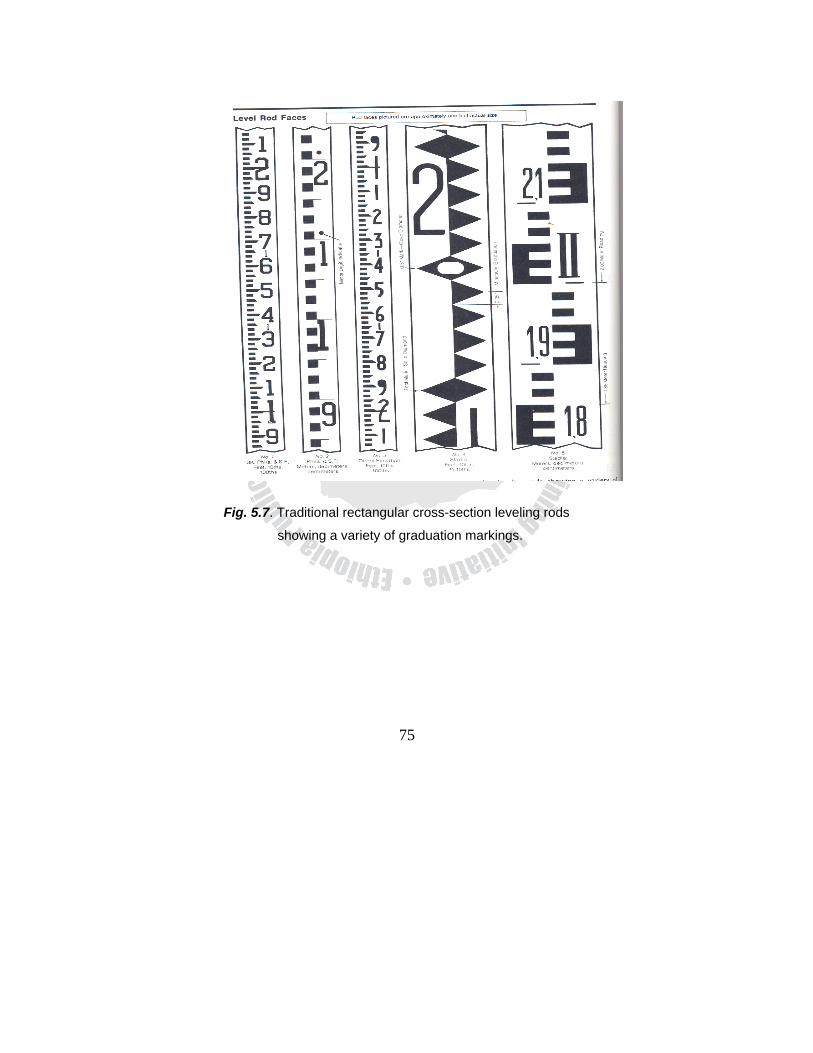
75
Fig. 5.7. Traditional rectangular cross-section leveling rods
showing a variety of graduation markings.
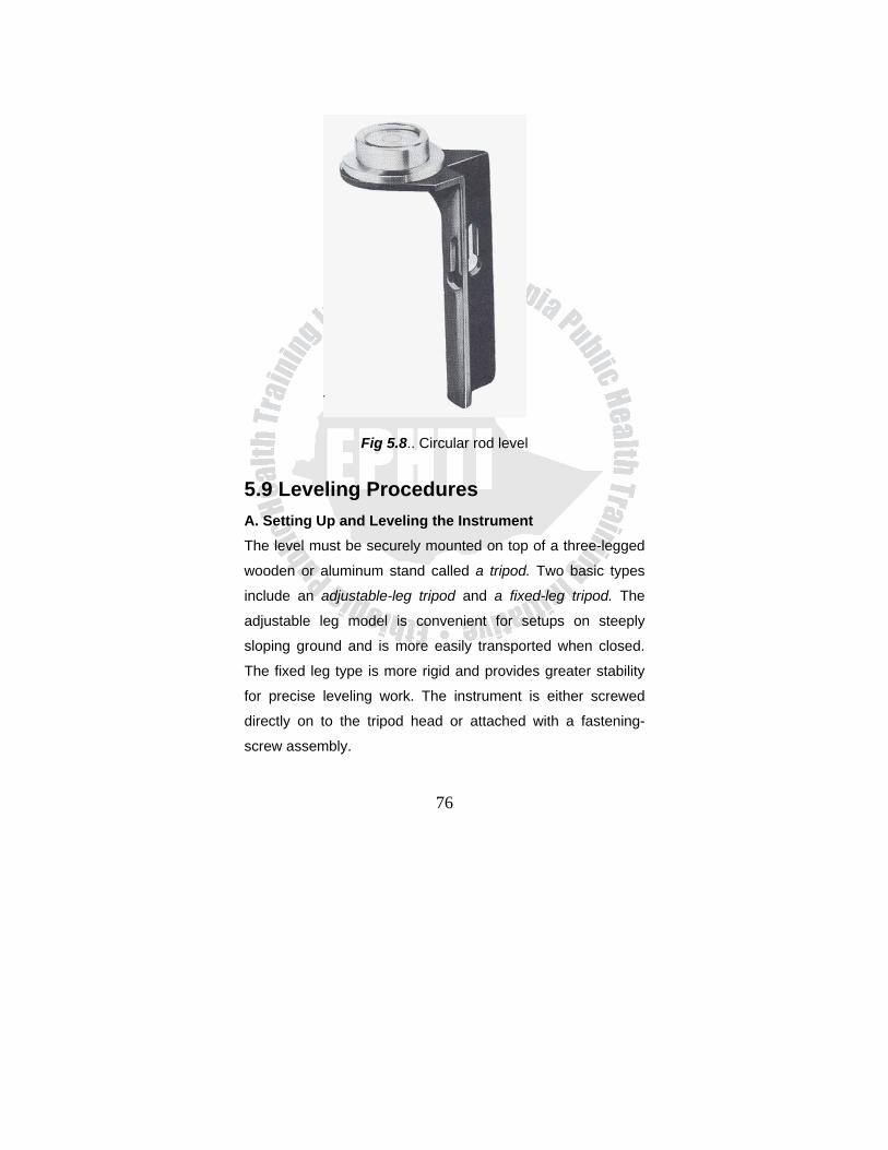
76
Fig 5.8.. Circular rod level
5.9 Leveling Procedures A. Setting Up and Leveling the Instrument The level must be securely mounted on top of a three-legged
wooden or aluminum stand called a tripod. Two basic types
include an adjustable-leg tripod and a fixed-leg tripod. The
adjustable leg model is convenient for setups on steeply
sloping ground and is more easily transported when closed.
The fixed leg type is more rigid and provides greater stability
for precise leveling work. The instrument is either screwed
directly on to the tripod head or attached with a fastening-
screw assembly.
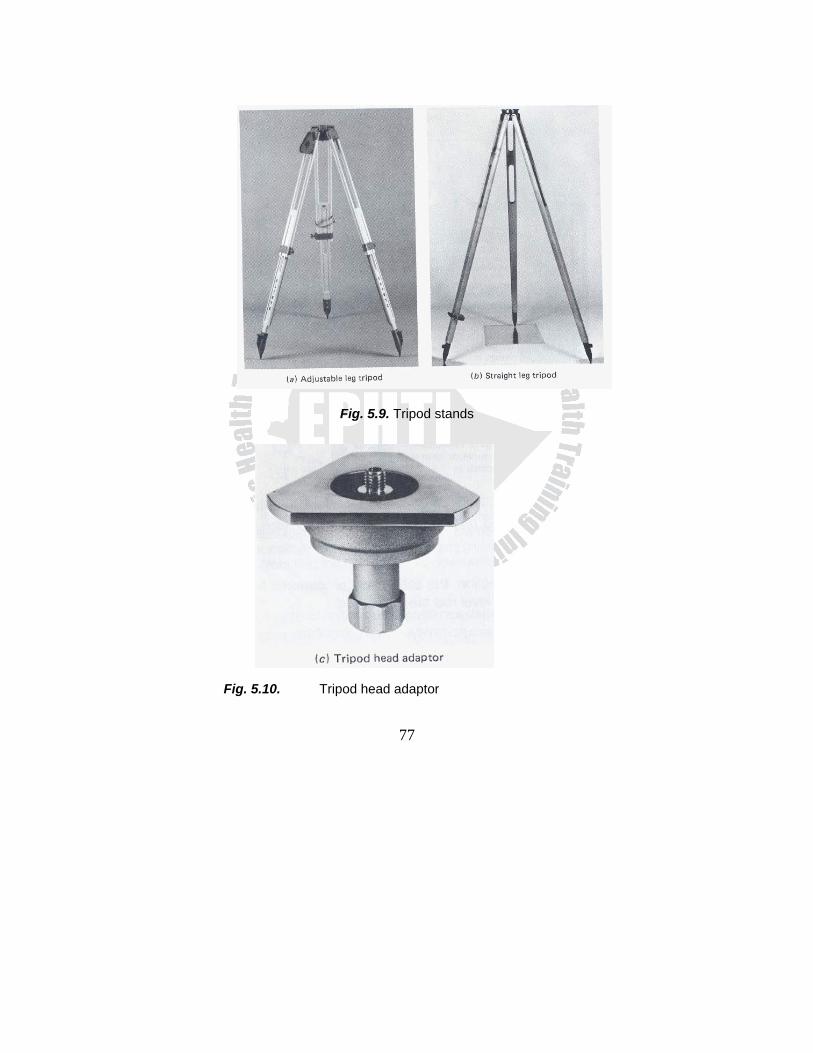
77
Fig. 5.9. Tripod stands
Fig. 5.10. Tripod head adaptor
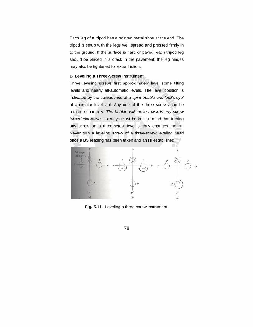
78
Each leg of a tripod has a pointed metal shoe at the end. The
tripod is setup with the legs well spread and pressed firmly in
to the ground. If the surface is hard or paved, each tripod leg
should be placed in a crack in the pavement; the leg hinges
may also be tightened for extra friction.
B. Leveling a Three-Screw Instrument Three leveling screws first approximately level some tilting
levels and nearly all-automatic levels. The level position is
indicated by the coincidence of a spirit bubble and 'bull's-eye'
of a circular level vial. Any one of the three screws can be
rotated separately. The bubble will move towards any screw
turned clockwise. It always must be kept in mind that turning
any screw on a three-screw level slightly changes the HI.
Never turn a leveling screw of a three-screw leveling head
once a BS reading has been taken and an HI established.
Fig. 5.11. Leveling a three-screw instrument.
79
C. Leveling Mistakes and Errors As with any surveying operation, blunders must be eliminated
and errors minimized while running levels. Misreading the rod
is a common blunder; it can be avoided by always having the
rod person check the reading with pencil point or target. Note-
keeping mistakes can be particularly troublesome. The
computations of HI and turning point (TP) elevation should be
done in the field, as the work progresses. A simple arithmetic
check at the end of the leveling run can be made to avoid
addition or subtraction errors.
a. Random Errors Unavoidable accidental errors may occur when running
levels, for several reasons. For example:
The level rod may not be precise when the reading is
taken.
Heat waves from the ground make it difficult to read.
On windy day, slight vibration of the cross hair can
cause small errors in the reading.
The instrument may be slightly out of level if the spirit
level is not perfectly centered.
Accidental errors can be minimized with a properly maintained
and adjusted instrument if the following steps are taken:
1. Make sure the tripod legs are secure and firmly anchored
before leveling the instrument.
80
2. Check to see that the bubble is centered before each
reading; re-center it if necessary.
3. Do not lean on the tripod legs when reading the rod.
4. Have the rod person use a rod level, to make sure it is
held vertically.
5. Try to keep the line of sight about 0.5m above the
ground when positioning the instrument.
6. Do not use very long BS and FS reading.
b. Systematic / Instrumental Errors Incorrect length of the rod.
When the bubble tube axis is not perpendicular to the
standing axis of the instrument
When the line of sight of the telescope is not parallel to
the bubble axis.
If the line of sight of a level is not exactly horizontal when the
bubble is centered, but slopes either up or down, it will slope
by the same amount for any direction of the telescope. As
long as the horizontal lengths of the BS and FS are the same,
from any given instrument position to the rod, the line of sight
will intercept the rod held on each point with exactly the same
error in height. But since one of the sights is a plus sight (+)
and other a minus sight (-), the two errors will cancel each
other out in the leveling computation.
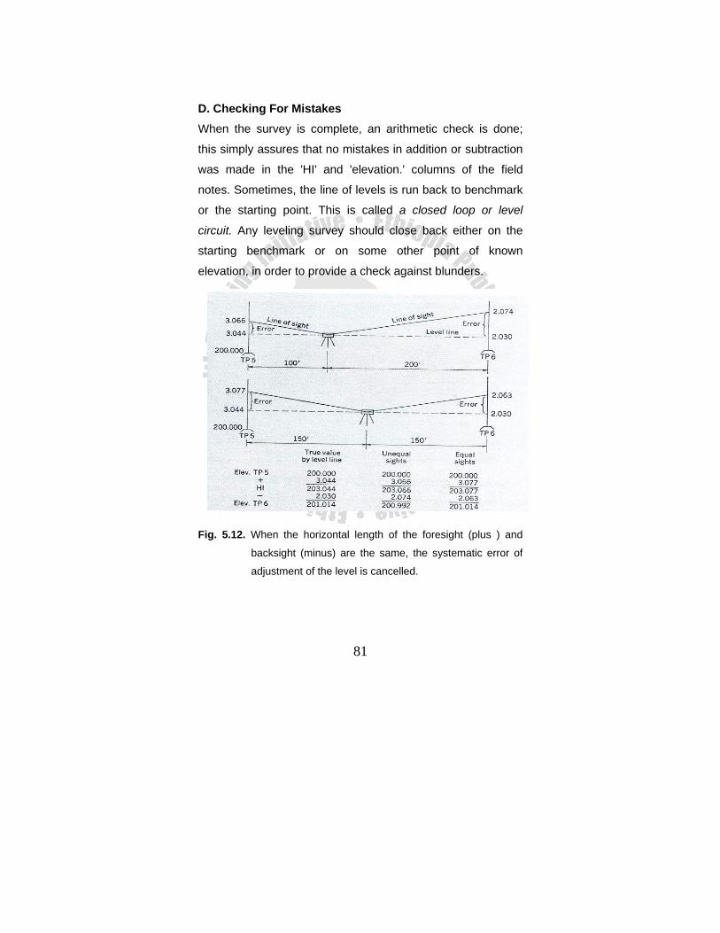
81
D. Checking For Mistakes When the survey is complete, an arithmetic check is done;
this simply assures that no mistakes in addition or subtraction
was made in the 'HI' and 'elevation.' columns of the field
notes. Sometimes, the line of levels is run back to benchmark
or the starting point. This is called a closed loop or level
circuit. Any leveling survey should close back either on the
starting benchmark or on some other point of known
elevation, in order to provide a check against blunders.
Fig. 5.12. When the horizontal length of the foresight (plus ) and
backsight (minus) are the same, the systematic error of
adjustment of the level is cancelled.
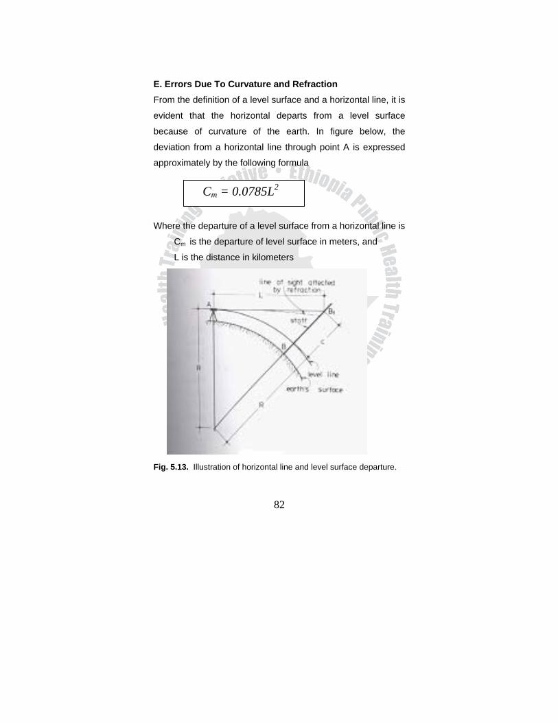
82
E. Errors Due To Curvature and Refraction
From the definition of a level surface and a horizontal line, it is
evident that the horizontal departs from a level surface
because of curvature of the earth. In figure below, the
deviation from a horizontal line through point A is expressed
approximately by the following formula
Where the departure of a level surface from a horizontal line is
Cm is the departure of level surface in meters, and
L is the distance in kilometers
Fig. 5.13. Illustration of horizontal line and level surface departure.
Cm = 0.0785L2
83
For horizontal sight, refraction Rm in meters is expressed by
the formula
The combined effect of curvature of the earth and refraction, h
is approximated as
Where hm is in meters.
For example, for a 100m length there is about 0.00067m
length of error.
3. Trigonometric Leveling Trigonometric leveling is an indirect procedure; the vertical
distances are computed from vertical angle and horizontal or
slope distance data. It is also applied for topo work over rough
terrain or other obstacles.
The difference in elevation between two points can be
determined by measuring
1. The inclined or horizontal distance between them and
2. The zenith angle or the vertical angle to one point from
the other
N.B: Zenith angles and Vertical angles are both measured in
a vertical plane. Zenith angles are measured down
ward from the vertical, and Vertical angles are
measured up or down from the horizontal.
Rm = 0.011L2
hm = 0.0675L2
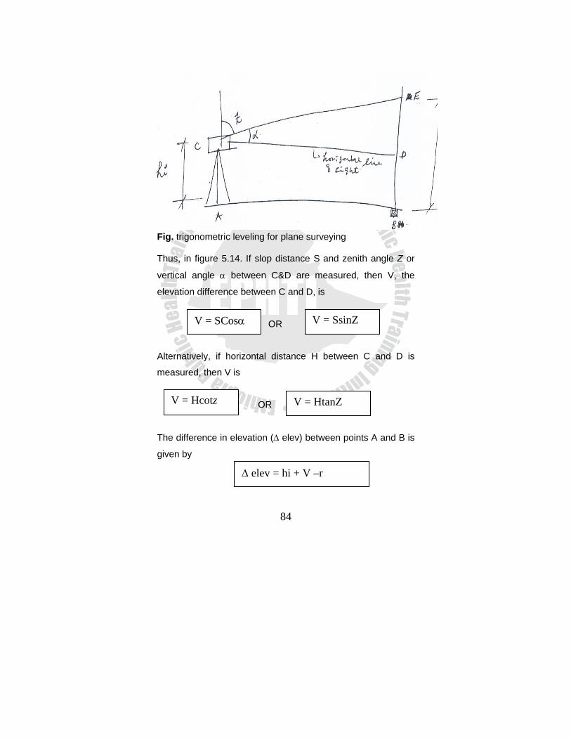
84
Fig. trigonometric leveling for plane surveying
Thus, in figure 5.14. If slop distance S and zenith angle Z or
vertical angle α between C&D are measured, then V, the
elevation difference between C and D, is
OR
Alternatively, if horizontal distance H between C and D is
measured, then V is
OR
The difference in elevation (Δ elev) between points A and B is
given by
V = SCosα V = SsinZ
V = Hcotz V = HtanZ
Δ elev = hi + V –r
85
Where hi is the height of the instrument above point A and r is
the reading on the rod held at B when zenith angle z or
vertical angle α is read. If r is made equal to hi, then these two
values cancel in equation above, and simplifies the
computations.
Note the distinction between HI and hi. Although both are
called Height of Instrument, HI is the elevation of the
instrument above datum, while hi is the height of the
instrument above an occupied point.
For shorter lines (up to about 1000ft or m in length) elevation
differences obtained in trigonometric leveling are appropriately
computed and depicted by the above equations. For longer
lines, however, earth curvature and refraction become factors
that must be considered. Fig. 5.15 illustrates the situation.
Here an instrument is set up at C over point A. Sight D is
made on a rod held at point B, and zenith angles zm or vertical
angles αm is measured. The true difference in elevation
between A and B is vertical distance HB between level lines
through A and B, which equal to HG + GF + V –ED –r. Since
HG is the instrument height hi, GF is earth curvature C, and
ED is refraction R, the elevation difference can be written as:
Δ elev = hi + V + (C-R) – r
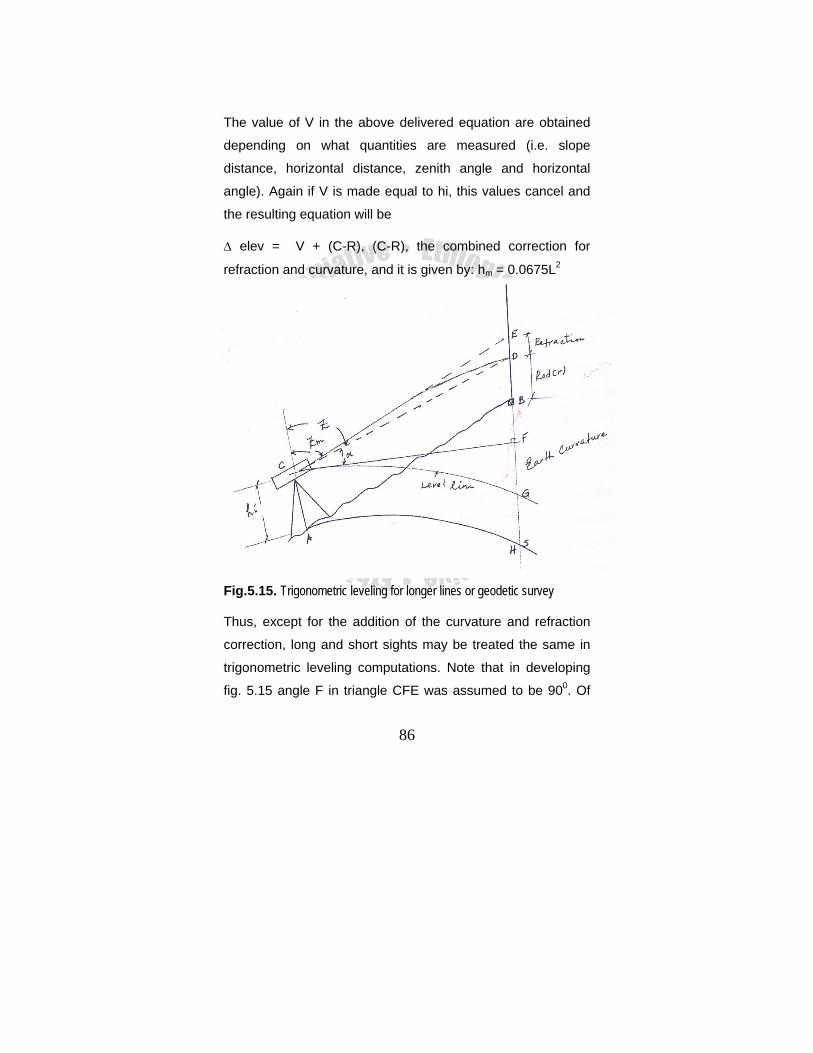
86
The value of V in the above delivered equation are obtained
depending on what quantities are measured (i.e. slope
distance, horizontal distance, zenith angle and horizontal
angle). Again if V is made equal to hi, this values cancel and
the resulting equation will be
Δ elev = V + (C-R), (C-R), the combined correction for
refraction and curvature, and it is given by: hm = 0.0675L2
Fig.5.15. Trigonometric leveling for longer lines or geodetic survey
Thus, except for the addition of the curvature and refraction
correction, long and short sights may be treated the same in
trigonometric leveling computations. Note that in developing
fig. 5.15 angle F in triangle CFE was assumed to be 900. Of
87
course as lines become extremely long, this assumption does
not hold. However, for lengths with in the practical range,
errors caused by this assumption are negligible.
The hi used in the equation , Δ elev = hi + V + (C-R) – r; can
be obtained by simply measuring the vertical distance from
the occupied point up to the instrument’s horizontal axis (axis
about which the telescope rotates ) using a graduated rod or
rule. An alternative method can be used to determine the
elevation of a point that produces accurate results and does
not require measurement of the hi. In this procedure, the
instrument is setup at a location where it is approximately
equidistant from a point of known elevation (Bench mark) and
the one whose elevation is to be determined. The slope
distance and zenith (or vertical) angle are measured to each
point. Because the distances from the two points are
approximately equal, the curvature and refraction errors
cancel. Since, the same instrument set up applies to both
readings, the hi values cancel, and if the same rod reading r is
sighted when making both angle readings, they cancel. Thus
the elevation of the unknown point is simply the bench mark
elevation, minus V calculated from the bench mark, plus V
computed for the unknown point, where the V values are
obtained using the above equations.
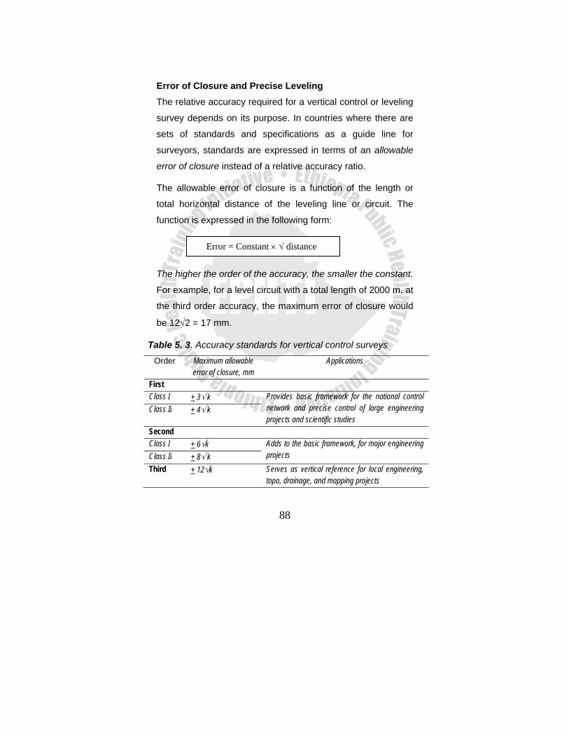
88
Error of Closure and Precise Leveling The relative accuracy required for a vertical control or leveling
survey depends on its purpose. In countries where there are
sets of standards and specifications as a guide line for
surveyors, standards are expressed in terms of an allowable
error of closure instead of a relative accuracy ratio.
The allowable error of closure is a function of the length or
total horizontal distance of the leveling line or circuit. The
function is expressed in the following form:
The higher the order of the accuracy, the smaller the constant.
For example, for a level circuit with a total length of 2000 m, at
the third order accuracy, the maximum error of closure would
be 12√2 = 17 mm.
Table 5. 3. Accuracy standards for vertical control surveys
Order Maximum allowable error of closure, mm
Applications
First Class I + 3√ k Provides basic framework for the national control
network and precise control of large engineering projects and scientific studies
Class II + 4√ k
Second Class I + 6√k Adds to the basic framework, for major engineering
projects Class II + 8√ k Third + 12√k Serves as vertical reference for local engineering,
topo, drainage, and mapping projects
Error = Constant × √ distance
89
Adjusting Benchmark Elevations The importance of running a line of levels back to the starting
benchmark, or to some other fixed point of known elevation is
to avoid blunders. There is really no way to assure that a
blunder was not made in the work with out closing the level
circuit one way or the other. It is much less expensive to find
and correct a blunder in the field by closing the loop than to
have to return and repeat the work at a later date.
When the line of levels or level circuit is completed, there is
usually some small difference between the given fixed
elevation of the benchmark and the observed elevation
arrived at in the leveling notes. If the arithmetic check works
out all right, then it may be assumed that the discrepancy is
due to random or accidental errors.
Suppose a leveling survey closes within the desired order and
class of accuracy; in other words, there is an error of closure,
but it is acceptable. The problem now is to distribute that total
error of closure among the various intermediate benchmarks
and to adjust the circuit so that it closes exactly. In doing this
for single level line or circuit, it may be assumed that the
elevation error at each point along the circuit or line of levels
is directly proportional to the distance of the point from the
starting benchmark. The relationships for adjusting the
leveling line or circuit may be summarized as follows:
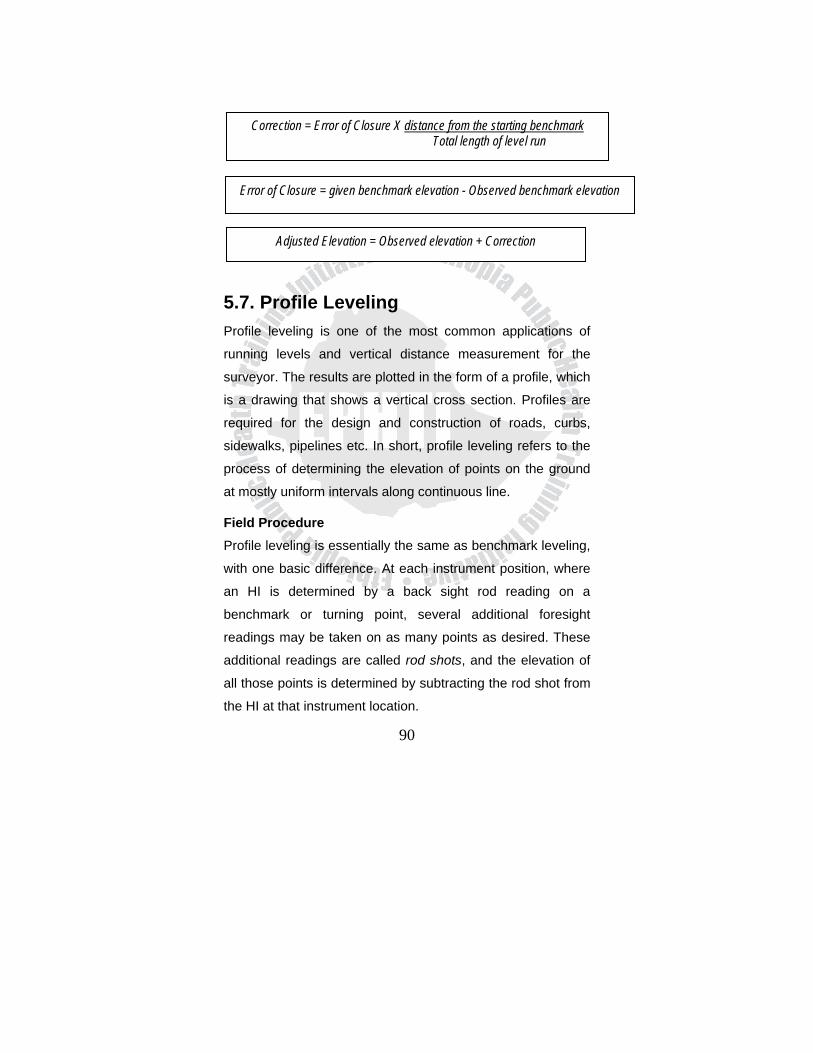
90
5.7. Profile Leveling Profile leveling is one of the most common applications of
running levels and vertical distance measurement for the
surveyor. The results are plotted in the form of a profile, which
is a drawing that shows a vertical cross section. Profiles are
required for the design and construction of roads, curbs,
sidewalks, pipelines etc. In short, profile leveling refers to the
process of determining the elevation of points on the ground
at mostly uniform intervals along continuous line.
Field Procedure Profile leveling is essentially the same as benchmark leveling,
with one basic difference. At each instrument position, where
an HI is determined by a back sight rod reading on a
benchmark or turning point, several additional foresight
readings may be taken on as many points as desired. These
additional readings are called rod shots, and the elevation of
all those points is determined by subtracting the rod shot from
the HI at that instrument location.
Error of Closure = given benchmark elevation - Observed benchmark elevation
Adjusted Elevation = Observed elevation + Correction
Correction = Error of Closure X distance from the starting benchmark Total length of level run
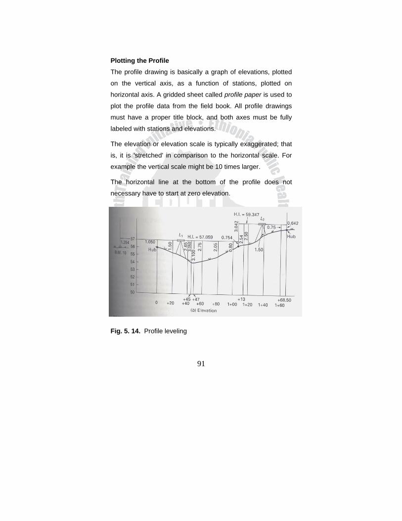
91
Plotting the Profile The profile drawing is basically a graph of elevations, plotted
on the vertical axis, as a function of stations, plotted on
horizontal axis. A gridded sheet called profile paper is used to
plot the profile data from the field book. All profile drawings
must have a proper title block, and both axes must be fully
labeled with stations and elevations.
The elevation or elevation scale is typically exaggerated; that
is, it is 'stretched' in comparison to the horizontal scale. For
example the vertical scale might be 10 times larger.
The horizontal line at the bottom of the profile does not
necessary have to start at zero elevation.
Fig. 5. 14. Profile leveling
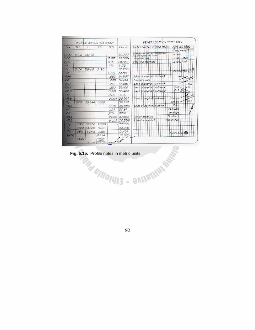
92
Fig. 5.15. Profile notes in metric units.

93
Fig. 5.16. Plotted profile.
5.8. Cross-Section Leveling The term cross-section generally refers to a relatively short
profile view of the ground, which is drawn perpendicular to the
route centerline of a highway or other types of linear projects.
Cross-sectional drawings are particularly important for
estimating the earthwork volumes needed to construct a
roadway; they show the existing ground elevations, the
proposed cut or fill side slopes, and the grade elevation for the
road base.
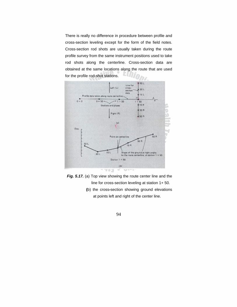
94
There is really no difference in procedure between profile and
cross-section leveling except for the form of the field notes.
Cross-section rod shots are usually taken during the route
profile survey from the same instrument positions used to take
rod shots along the centerline. Cross-section data are
obtained at the same locations along the route that are used
for the profile rod-shot stations.
Fig. 5.17. (a) Top view showing the route center line and the
line for cross-section leveling at station 1+ 50.
(b) the cross-section showing ground elevations
at points left and right of the center line.
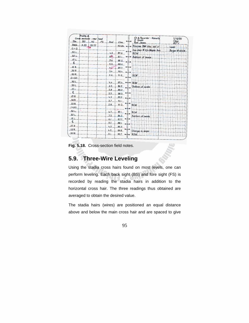
95
Fig. 5.18. Cross-section field notes.
5.9. Three-Wire Leveling Using the stadia cross hairs found on most levels, one can
perform leveling. Each back sight (BS) and fore sight (FS) is
recorded by reading the stadia hairs in addition to the
horizontal cross hair. The three readings thus obtained are
averaged to obtain the desired value.
The stadia hairs (wires) are positioned an equal distance
above and below the main cross hair and are spaced to give
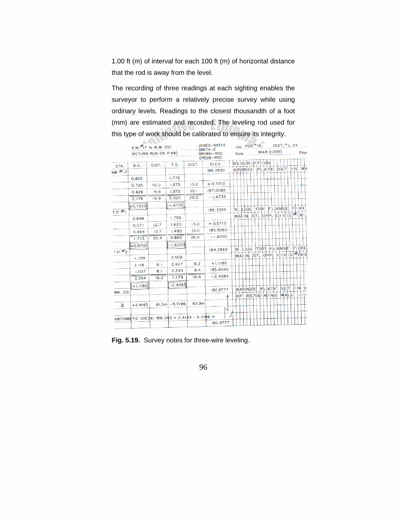
96
1.00 ft (m) of interval for each 100 ft (m) of horizontal distance
that the rod is away from the level.
The recording of three readings at each sighting enables the
surveyor to perform a relatively precise survey while using
ordinary levels. Readings to the closest thousandth of a foot
(mm) are estimated and recorded. The leveling rod used for
this type of work should be calibrated to ensure its integrity.
Fig. 5.19. Survey notes for three-wire leveling.
97
Exercise 1. A differential leveling loop began and closed on BM
bridge (elevation 1237.28 ft). The BS and FS distances
were kept approximately equal. Readings taken in order
are 8.59 on BM bridge, 6.54 and 4.87 on TP1, 7.50 and
6.08 on BM X, 7.23 and 2.80 on TP2, and 1.11 on BM
bridge. Prepare, check and adjust the notes.
2. A level setup midway between X and Y reads 5.18 on X
and 6.80 on Y. When moved within a few feet of X,
readings of 4.74 on X and 6.32 on Y are recorded. What
is the true elevation difference, and the reading required
on Y to adjust the instrument?
3. Reciprocal leveling gives the following readings in feet
from setup near A: on A, 2.071; on B, 8.254, 8.259 and
8.257. At the setup near B, 9.112; on A, 2.926, 2.930, and
2.927. The elevation of B is 1099.60. Compute the
misclosure and the elevation of A.
4. Prepare a set of three-wire leveling notes for the data
given and make the page check. The elevation of BM X is
230.054m. Rod readings(in meter) are:
BS on BM X: H = 1.683, M = 1.453, L = 1.224: FS on
TP1: H = 2.959, M = 2.707, L = 2.454; BS on
TP1: H = 2.254, M = 2.054, L = 1.854; FS on
BM Y: H = 1.013, M = 0.817, L = 0.620.
98
5. Prepare a set of profile leveling notes for the data listed
and show the page check. The elevation of BM A is
1275.39 ft, and the elevation of BM B is 1264.78 ft. Rod
readings are: BS on BM A, 5.68; IFS on 1+00, 4.3; FS on
TP1, 9.56; BS on TP1,10.02; IFS on 2+00,11.1;on 3+00,
6.1; FS on TP2,8.15;BS on TP2, 3.28; ifs on 3+64,1.51;
on 4+00, 3.1;on 5+00, 6.4; FS on TP3, 7.77; BS on TP3,
3.16; FS on BM B, 7.23.
6. If the elevation on a certain project at stations 10+00 and
14+00 are 1232.47 and 1248.06, respectively, what is the
percent grade connecting these points?
7. In trigonometric leveling from point A to point B, the slope
distance and zenith angle measured at A were 23051.82
ft and 83041'16". At B these measurements were
23051.85ft and 96021'31", respectively. If the instrument
and rod target height were equal, calculate the difference
in elevation from A to B.
8. Prepare a set of profile leveling notes for the survey
illustrated. In addition to computing all elevations, show
the arithmetic check and the resulting error of closure.
And plot the profile graph with appropriate scale.
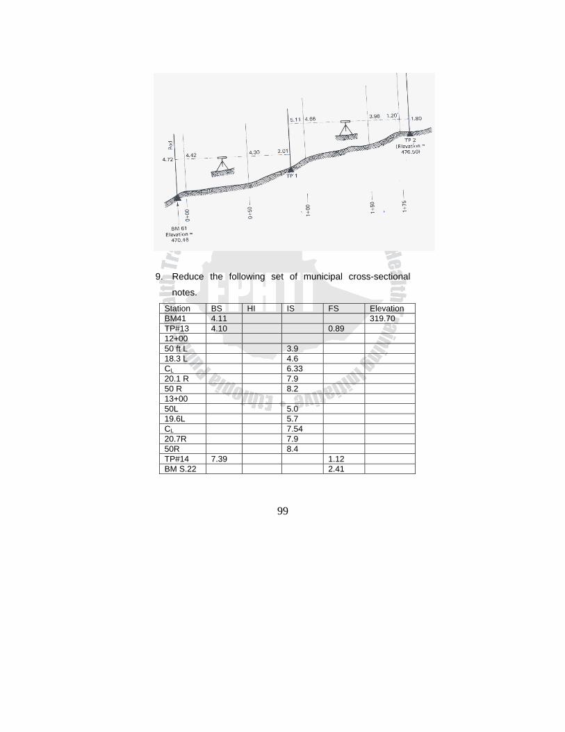
99
9. Reduce the following set of municipal cross-sectional
notes.
Station BS HI IS FS Elevation BM41 4.11 319.70 TP#13 4.10 0.89 12+00 50 ft L 3.9 18.3 L 4.6 CL 6.33 20.1 R 7.9 50 R 8.2 13+00 50L 5.0 19.6L 5.7 CL 7.54 20.7R 7.9 50R 8.4 TP#14 7.39 1.12 BM S.22 2.41
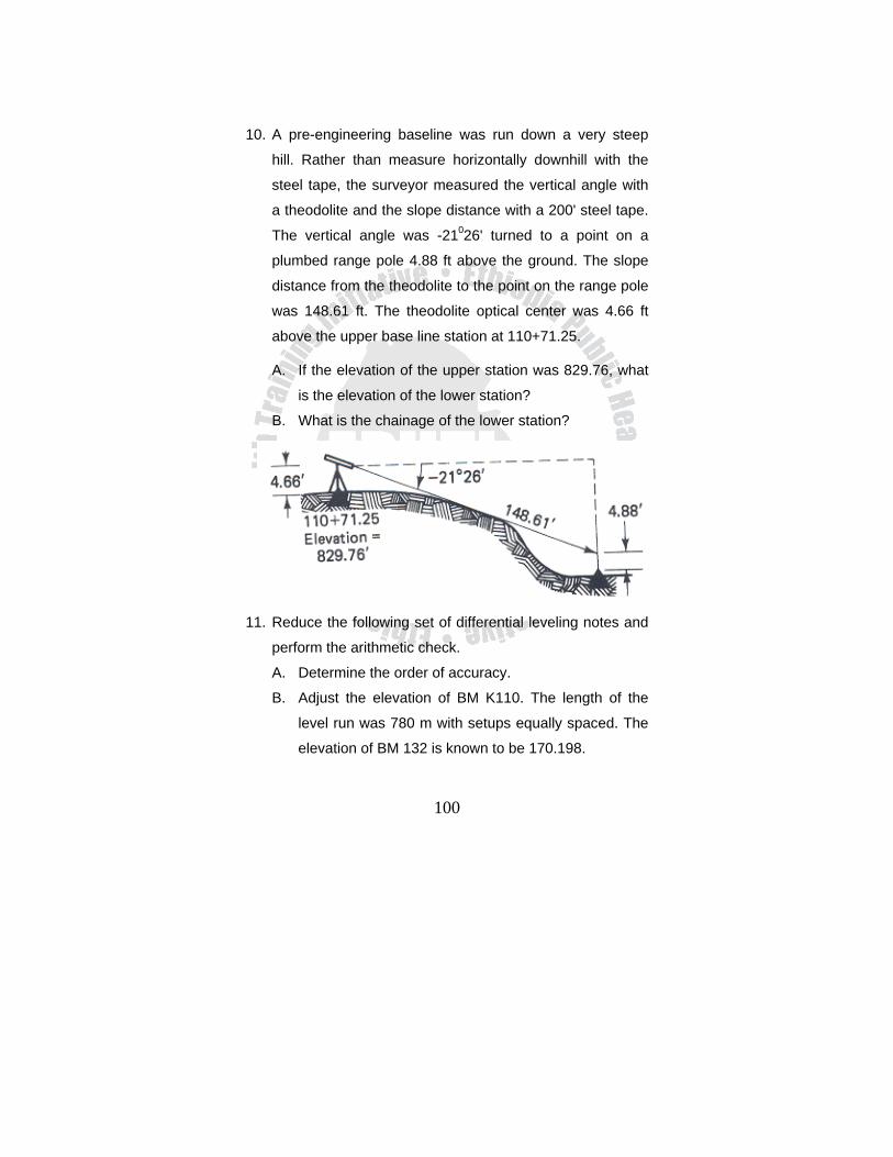
100
10. A pre-engineering baseline was run down a very steep
hill. Rather than measure horizontally downhill with the
steel tape, the surveyor measured the vertical angle with
a theodolite and the slope distance with a 200' steel tape.
The vertical angle was -21026' turned to a point on a
plumbed range pole 4.88 ft above the ground. The slope
distance from the theodolite to the point on the range pole
was 148.61 ft. The theodolite optical center was 4.66 ft
above the upper base line station at 110+71.25.
A. If the elevation of the upper station was 829.76, what
is the elevation of the lower station?
B. What is the chainage of the lower station?
11. Reduce the following set of differential leveling notes and
perform the arithmetic check.
A. Determine the order of accuracy.
B. Adjust the elevation of BM K110. The length of the
level run was 780 m with setups equally spaced. The
elevation of BM 132 is known to be 170.198.
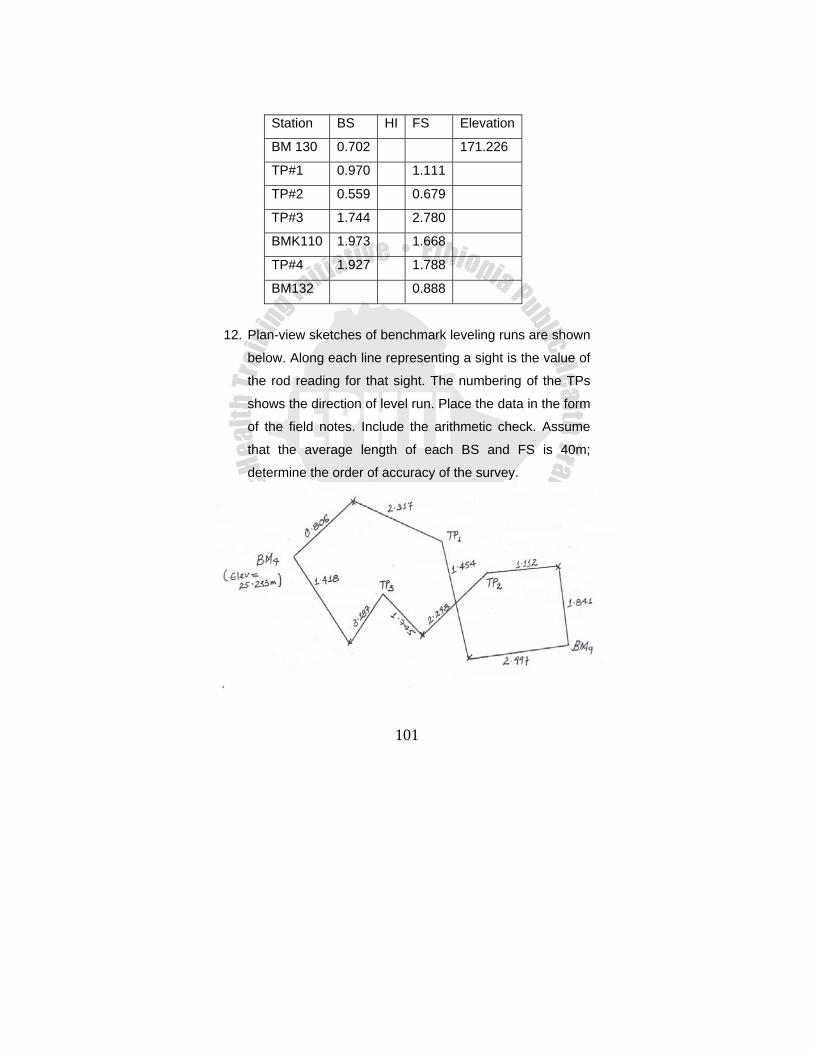
101
Station BS HI FS Elevation
BM 130 0.702 171.226
TP#1 0.970 1.111
TP#2 0.559 0.679
TP#3 1.744 2.780
BMK110 1.973 1.668
TP#4 1.927 1.788
BM132 0.888
12. Plan-view sketches of benchmark leveling runs are shown
below. Along each line representing a sight is the value of
the rod reading for that sight. The numbering of the TPs
shows the direction of level run. Place the data in the form
of the field notes. Include the arithmetic check. Assume
that the average length of each BS and FS is 40m;
determine the order of accuracy of the survey.

102
CHAPTER SIX TACHEOMETRY
6.1 LEARNING OBJECTIVES
At the end of this chapter, the student will be able to:
1. Define and state the principles of stadia
2. Measure distance and angles with the stadia principle
3. Identify potential sources of errors
4. Take corrective actions for identified errors.
6.2 Introduction The stadium (Tacheometry) is a rapid and efficient way of
indirectly measuring distances and elevation differences. The
accuracy attainable with stadia is suitable for lower order
trigonometric leveling, locating topographic details for
mapping, measuring lengths of back sights and fore sights in
differential leveling, and making quick checks of
measurements made by higher order methods.
6.3. Principles of Stadia In addition to the center horizontal cross hair, a theodolite or
transit reticles for stadia work has two additional horizontal
cross hairs spaced equidistant from the center one. With the
line of sight horizontal and directed towards a graduated rod
held vertically at a point some distance away, the interval
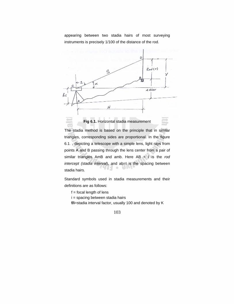
103
appearing between two stadia hairs of most surveying
instruments is precisely 1/100 of the distance of the rod.
Fig 6.1. Horizontal stadia measurement
The stadia method is based on the principle that in similar
triangles, corresponding sides are proportional. In the figure
6.1. , depicting a telescope with a simple lens, light rays from
points A and B passing through the lens center from a pair of
similar triangles AmB and amb. Here AB = I is the rod
intercept (stadia interval), and ab=I is the spacing between
stadia hairs.
Standard symbols used in stadia measurements and their
definitions are as follows:
f = focal length of lens i = spacing between stadia hairs f/i=stadia interval factor, usually 100 and denoted by K
104
I=rod intercept, also called stadia interval c=distance from instrument center (vertical axis) to
objective lens center. C=stadia factor=c+f d=distance from focal point F in front of the telescope to
face of the rod. D=distance from instrument center to face = C+d
From similarity of triangles,
or
Thus,
The objective lens of an internal focusing telescope remains
fixed in position, while a movable negative focusing lens
between the objective lens and the planes of the cross-hairs
change direction of the light rays. As a result, the stadia
constant ‘C’, is so small that it can be assumed equal to zero
and drop out. Thus the equation for distance on a horizontal
stadia sight reduces to:
D = KI
To determine the stadia factor K, rod intercept I for a
horizontal sight of known distance D is read.
d/f =I/I d = I(f/i) = KI
D = KI + C
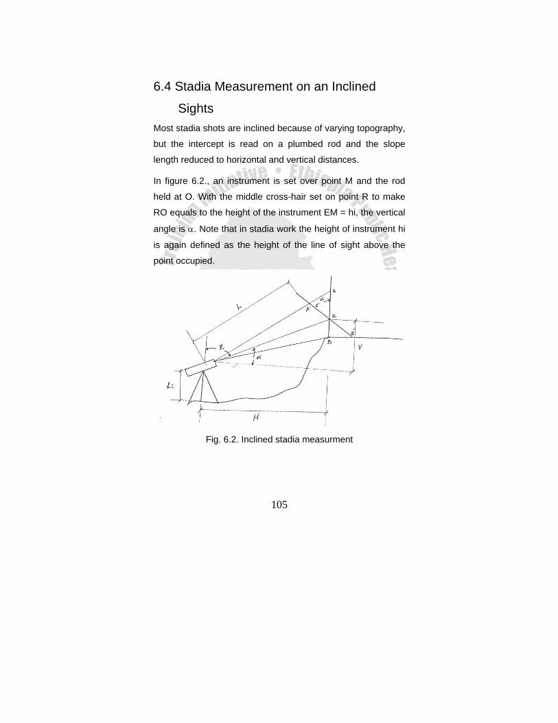
105
6.4 Stadia Measurement on an Inclined
Sights Most stadia shots are inclined because of varying topography,
but the intercept is read on a plumbed rod and the slope
length reduced to horizontal and vertical distances.
In figure 6.2., an instrument is set over point M and the rod
held at O. With the middle cross-hair set on point R to make
RO equals to the height of the instrument EM = hi, the vertical
angle is α. Note that in stadia work the height of instrument hi
is again defined as the height of the line of sight above the
point occupied.
Fig. 6.2. Inclined stadia measurment
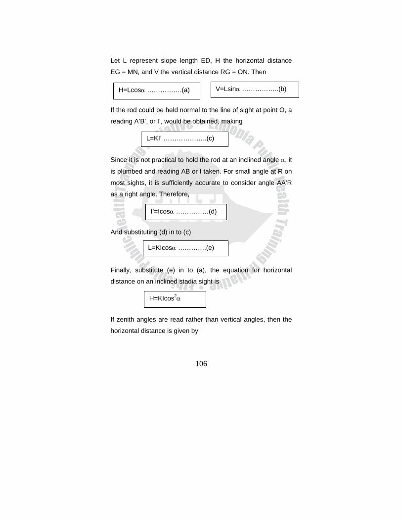
106
Let L represent slope length ED, H the horizontal distance
EG = MN, and V the vertical distance RG = ON. Then
If the rod could be held normal to the line of sight at point O, a
reading A’B’, or I’, would be obtained, making
Since it is not practical to hold the rod at an inclined angle α, it
is plumbed and reading AB or I taken. For small angle at R on
most sights, it is sufficiently accurate to consider angle AA’R
as a right angle. Therefore,
And substituting (d) in to (c)
Finally, substitute (e) in to (a), the equation for horizontal
distance on an inclined stadia sight is
If zenith angles are read rather than vertical angles, then the
horizontal distance is given by
H=Lcosα …………….(a) V=Lsinα ……………..(b)
L=KI’ ………………..(c)
I’=Icosα ……………(d)
L=KIcosα ………….(e)
H=KIcos2α
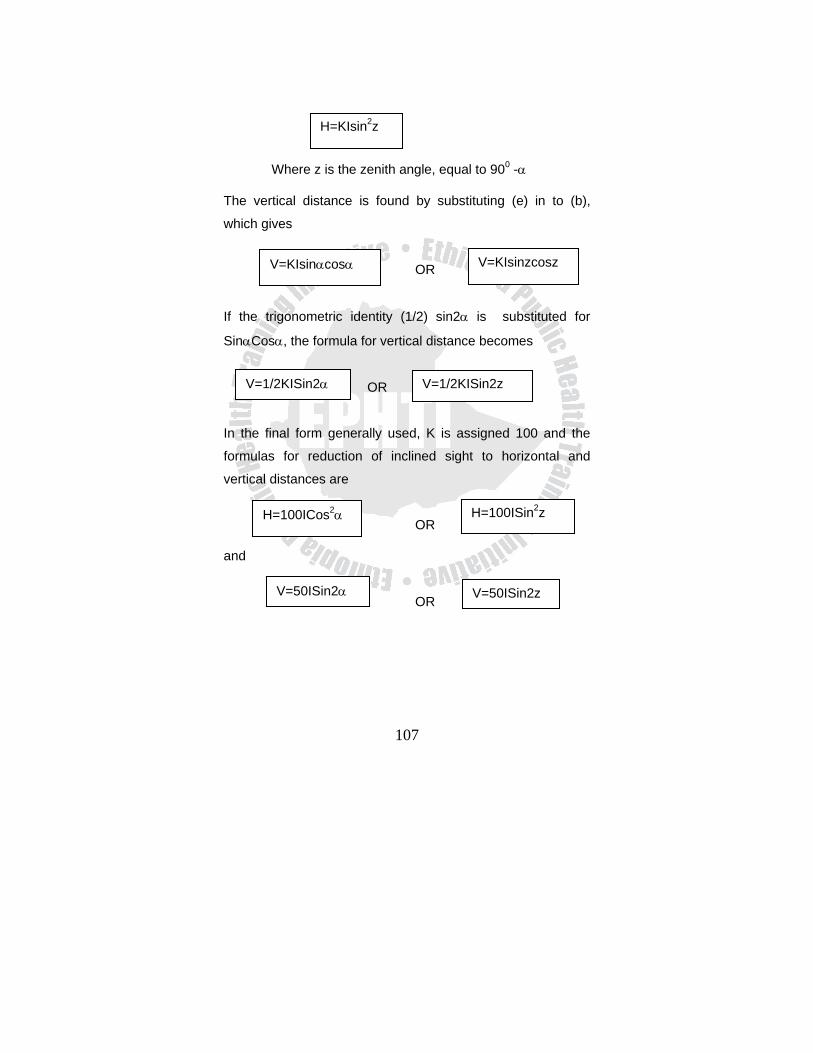
107
Where z is the zenith angle, equal to 900 -α
The vertical distance is found by substituting (e) in to (b),
which gives
OR
If the trigonometric identity (1/2) sin2α is substituted for
SinαCosα, the formula for vertical distance becomes
OR
In the final form generally used, K is assigned 100 and the
formulas for reduction of inclined sight to horizontal and
vertical distances are
OR
and
OR
H=KIsin2z
V=KIsinαcosα V=KIsinzcosz
V=1/2KISin2α V=1/2KISin2z
H=100ICos2α H=100ISin2z
V=50ISin2α V=50ISin2z
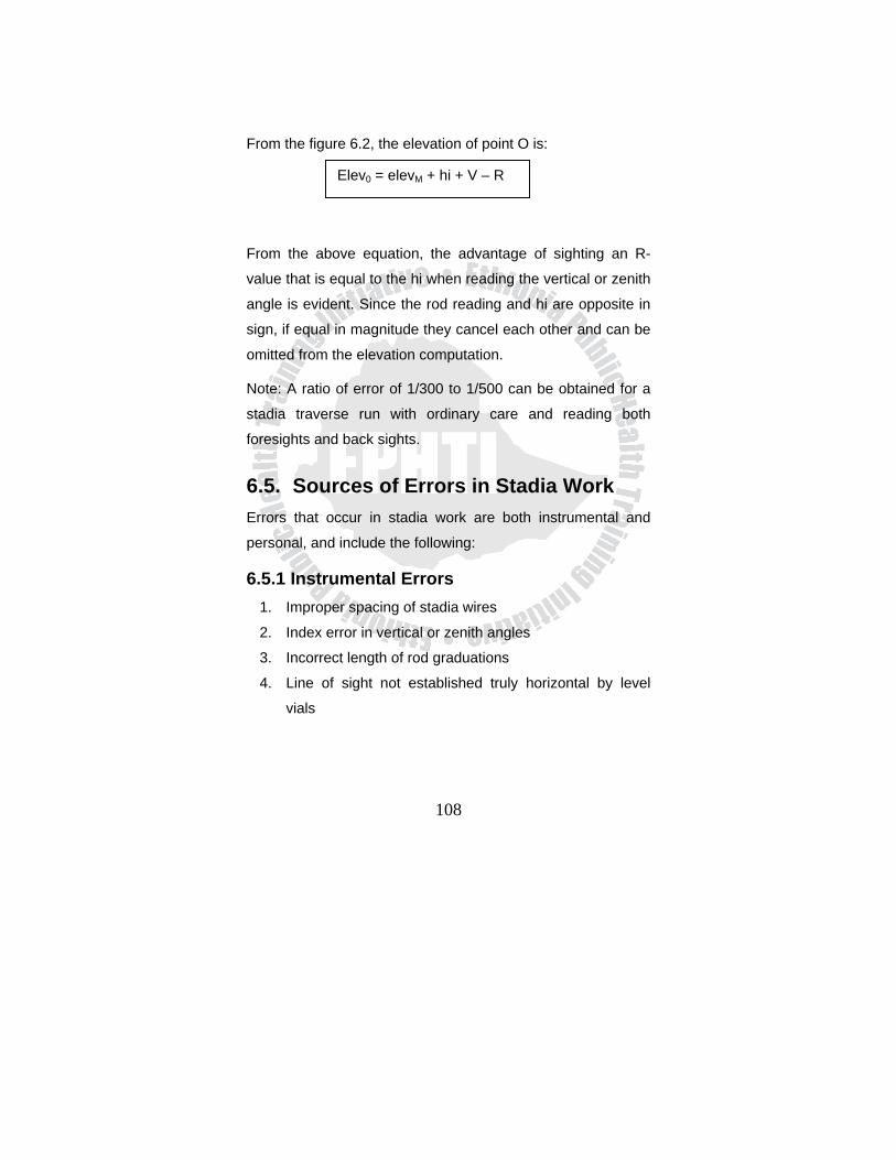
108
From the figure 6.2, the elevation of point O is:
From the above equation, the advantage of sighting an R-
value that is equal to the hi when reading the vertical or zenith
angle is evident. Since the rod reading and hi are opposite in
sign, if equal in magnitude they cancel each other and can be
omitted from the elevation computation.
Note: A ratio of error of 1/300 to 1/500 can be obtained for a
stadia traverse run with ordinary care and reading both
foresights and back sights.
6.5. Sources of Errors in Stadia Work Errors that occur in stadia work are both instrumental and
personal, and include the following:
6.5.1 Instrumental Errors 1. Improper spacing of stadia wires
2. Index error in vertical or zenith angles
3. Incorrect length of rod graduations
4. Line of sight not established truly horizontal by level
vials
Elev0 = elevM + hi + V – R

109
6.5.2 Personal Errors 1. Rod not held plumb (avoid by using a rod level)
2. Incorrect rod reading resulting from long sights
3. Careless leveling for vertical-arc readings
4. Mistakes:
a) Mistakes in reading the rod intercept
b) Use of an incorrect stadia interval factor
c) Waving the rod
d) Index error applied with wrong sign
e) Confusion of plus and minus vertical angles read
with a transit.
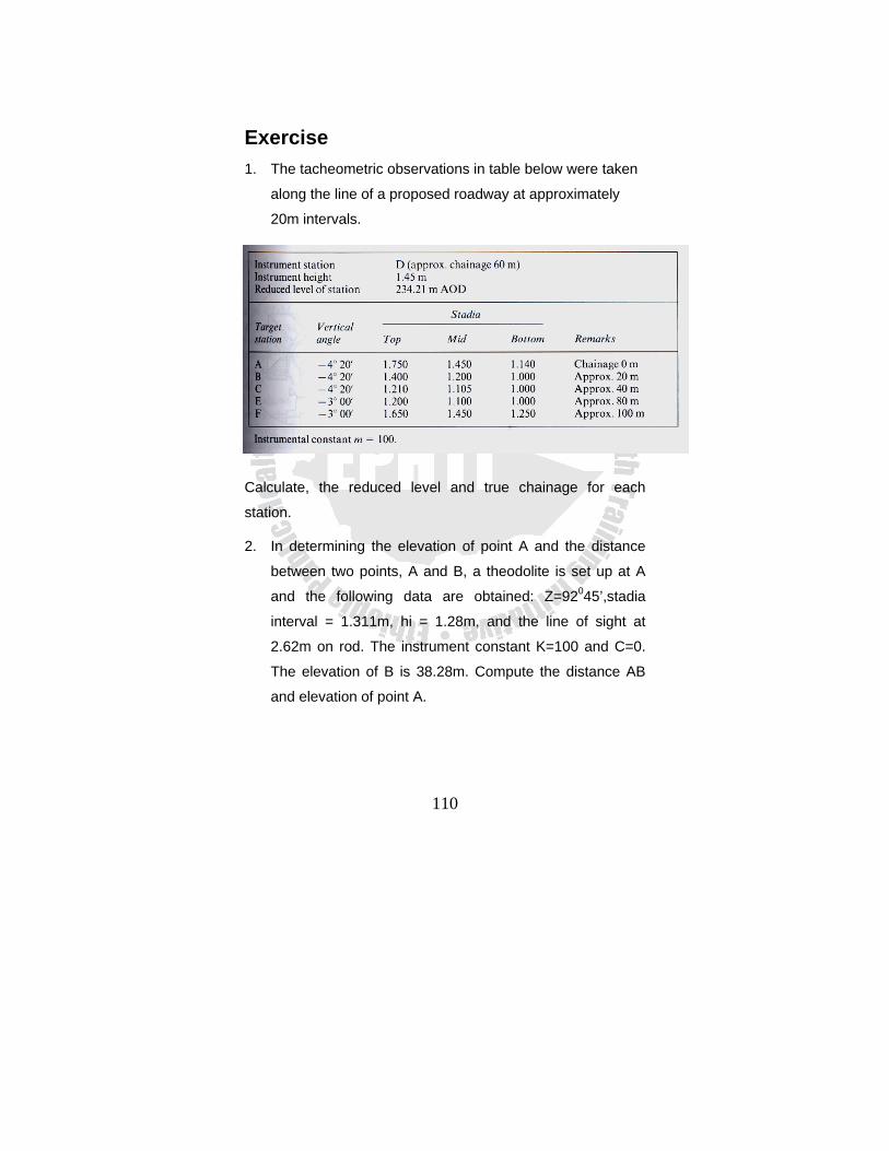
110
Exercise 1. The tacheometric observations in table below were taken
along the line of a proposed roadway at approximately
20m intervals.
Calculate, the reduced level and true chainage for each
station.
2. In determining the elevation of point A and the distance
between two points, A and B, a theodolite is set up at A
and the following data are obtained: Z=92045’,stadia
interval = 1.311m, hi = 1.28m, and the line of sight at
2.62m on rod. The instrument constant K=100 and C=0.
The elevation of B is 38.28m. Compute the distance AB
and elevation of point A.
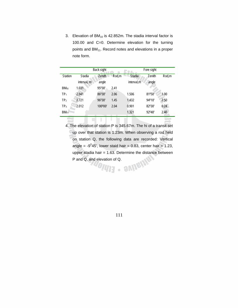
111
3. Elevation of BM10 is 42.852m. The stadia interval factor is
100.00 and C=0. Determine elevation for the turning
points and BM11. Record notes and elevations in a proper
note form.
Back sight Fore sight
Station Stadia interval, m
Zenith angle
Rod,m Stadia interval,m
Zenith angle
Rod,m
BM10 1.031 95030’ 2.41 TP1 2.041 86030’ 2.06 1.506 81050’ 1.00 TP2 2.721 96030’ 1.45 1.432 94010’ 2.50 TP3 2.012 100000’ 2.04 0.901 82030’ 0.24 BM11 1.321 92040’ 2.40
4. The elevation of station P is 345.67m. The hi of a transit set
up over that station is 1.23m. When observing a rod held
on station Q, the following data are recorded: Vertical
angle = -9045’, lower staid hair = 0.83, center hair = 1.23,
upper stadia hair = 1.63. Determine the distance between
P and Q, and elevation of Q.
112
CHAPTER SEVEN ANGLES, BEARING AND AZIMUTHS
7.1 Learning objectives At the end of this chapter, the student will be able to:
1. Define the different types of angles with their instrument
and unit of measurements.
2. Describe different meridians and system of designating
direction of lines.
3. Explain magnetic declination and local attraction
phenomena.
7.2. Introduction Determining the locations of points and orientations of lines
frequently depends on measurements of angles and
directions. In surveying, directions are given by bearings and
azimuths.
7.3 Angles Depending on the plane in which they are measured, angles
are classified as
Horizontal angles
- Basic measurement for determining bearing and
azimuths.
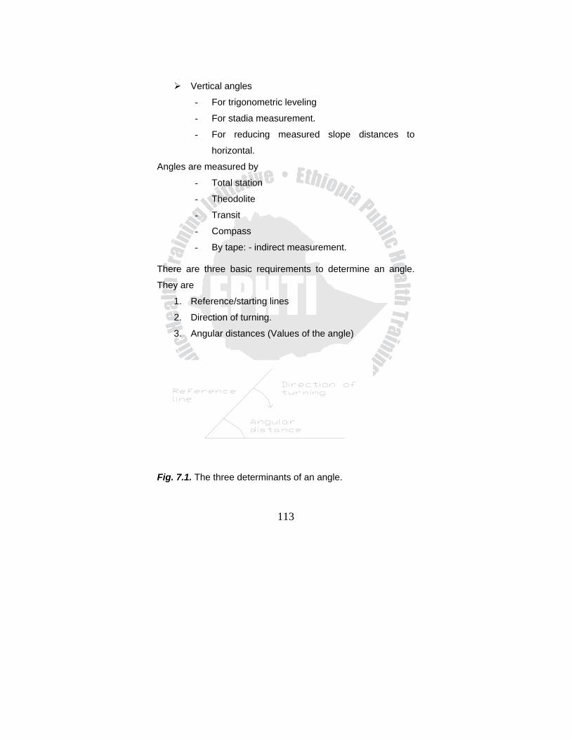
113
Vertical angles
- For trigonometric leveling
- For stadia measurement.
- For reducing measured slope distances to
horizontal.
Angles are measured by
- Total station
- Theodolite
- Transit
- Compass
- By tape: - indirect measurement.
There are three basic requirements to determine an angle.
They are
1. Reference/starting lines
2. Direction of turning.
3. Angular distances (Values of the angle)
Fig. 7.1. The three determinants of an angle.
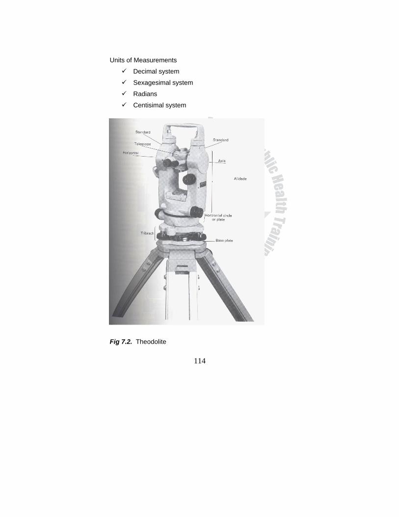
114
Units of Measurements
Decimal system
Sexagesimal system
Radians
Centisimal system
Fig 7.2. Theodolite

115
Fig 7.3. Horizontal circle reading using optical micrometer
• Kinds of Horizontal Angles The kinds of horizontal angles most commonly measured in
surveying are:
1. Interior angles.
2. Angles to the right.
3. Deflection angles.
1. Interior Angles They are measured on the inside of a closed
polygon.
Normally the angle at the apex with in a polygon is
measured.
Then a check can be made on their value because
the sum of all angles equals (n-2)180
Polygons (closed traverse) commonly used for
boundary surveys.
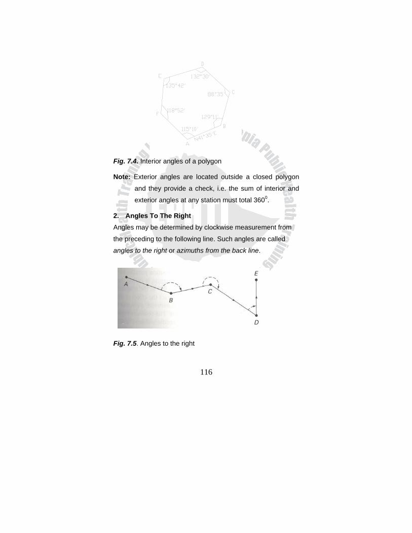
116
Fig. 7.4. Interior angles of a polygon
Note: Exterior angles are located outside a closed polygon
and they provide a check, i.e. the sum of interior and
exterior angles at any station must total 3600.
2. Angles To The Right Angles may be determined by clockwise measurement from
the preceding to the following line. Such angles are called
angles to the right or azimuths from the back line.
Fig. 7.5. Angles to the right
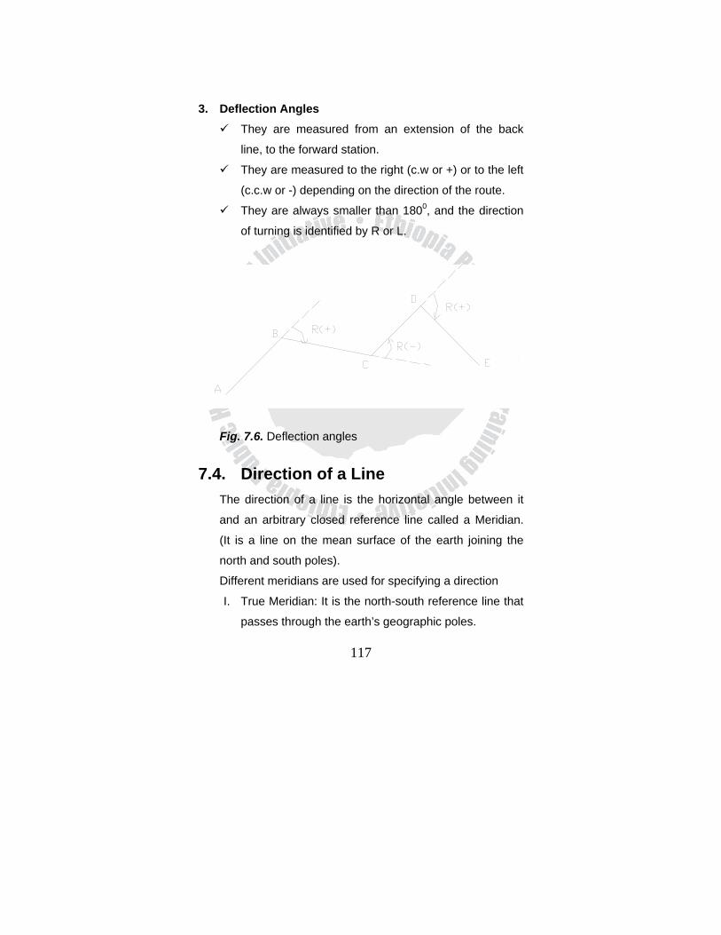
117
3. Deflection Angles
They are measured from an extension of the back
line, to the forward station.
They are measured to the right (c.w or +) or to the left
(c.c.w or -) depending on the direction of the route.
They are always smaller than 1800, and the direction
of turning is identified by R or L.
Fig. 7.6. Deflection angles
7.4. Direction of a Line The direction of a line is the horizontal angle between it
and an arbitrary closed reference line called a Meridian.
(It is a line on the mean surface of the earth joining the
north and south poles).
Different meridians are used for specifying a direction
I. True Meridian: It is the north-south reference line that
passes through the earth’s geographic poles.
118
II. Magnetic Meridians: defined by a freely suspended
magnetic needle that is influenced by earth’s
magnetic field only.
III. An Assumed Meridian: can be established by merely
assigning any arbitrary directions. For example, taking
certain street line to be true north.
7.4.1 Bearings Represent one system for designating directions of
lines.
A bearing is defined as the acute horizontal angle
between a reference meridian and the line.
The angle is measured from either the north or south
towards the east or west, to give a reading smaller than
900
True bearings/Magnetic bearings/Assumed bearings
are measured from True /Magnetic/Assumed meridians.
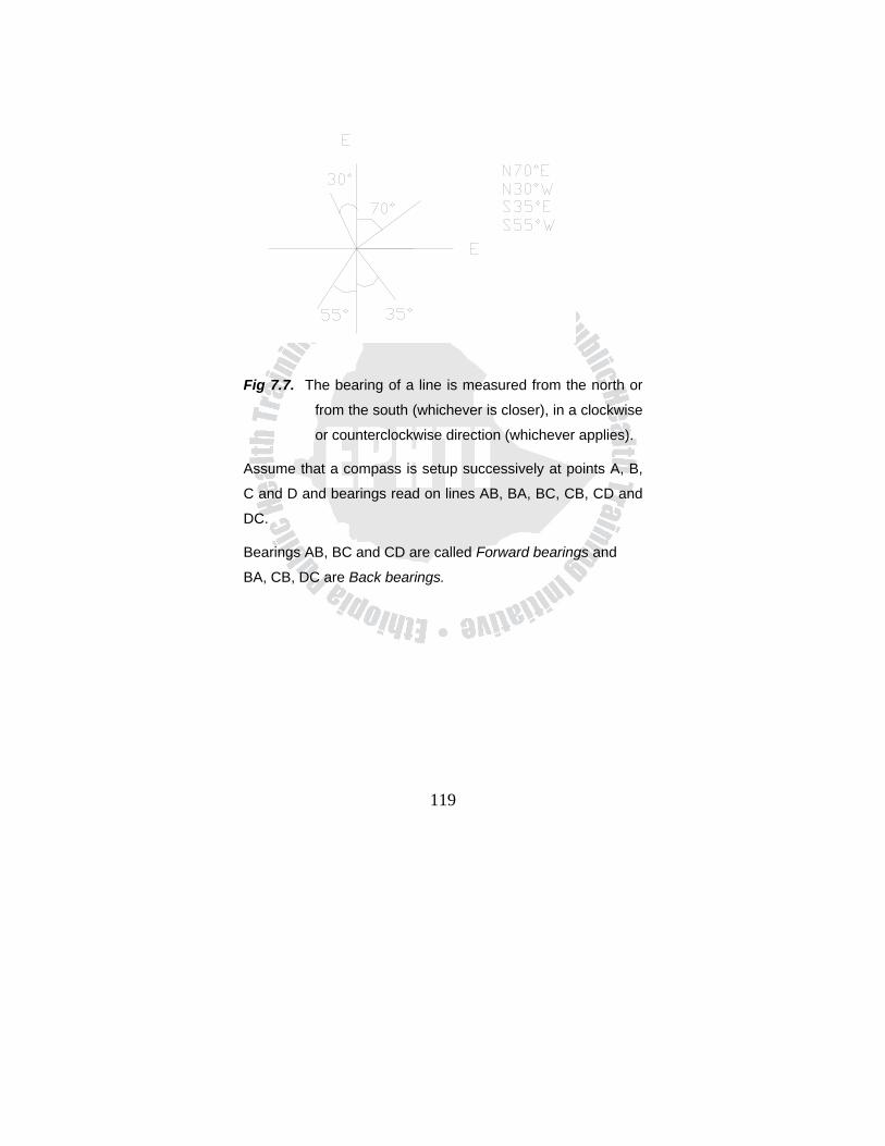
119
Fig 7.7. The bearing of a line is measured from the north or
from the south (whichever is closer), in a clockwise
or counterclockwise direction (whichever applies).
Assume that a compass is setup successively at points A, B,
C and D and bearings read on lines AB, BA, BC, CB, CD and
DC.
Bearings AB, BC and CD are called Forward bearings and
BA, CB, DC are Back bearings.
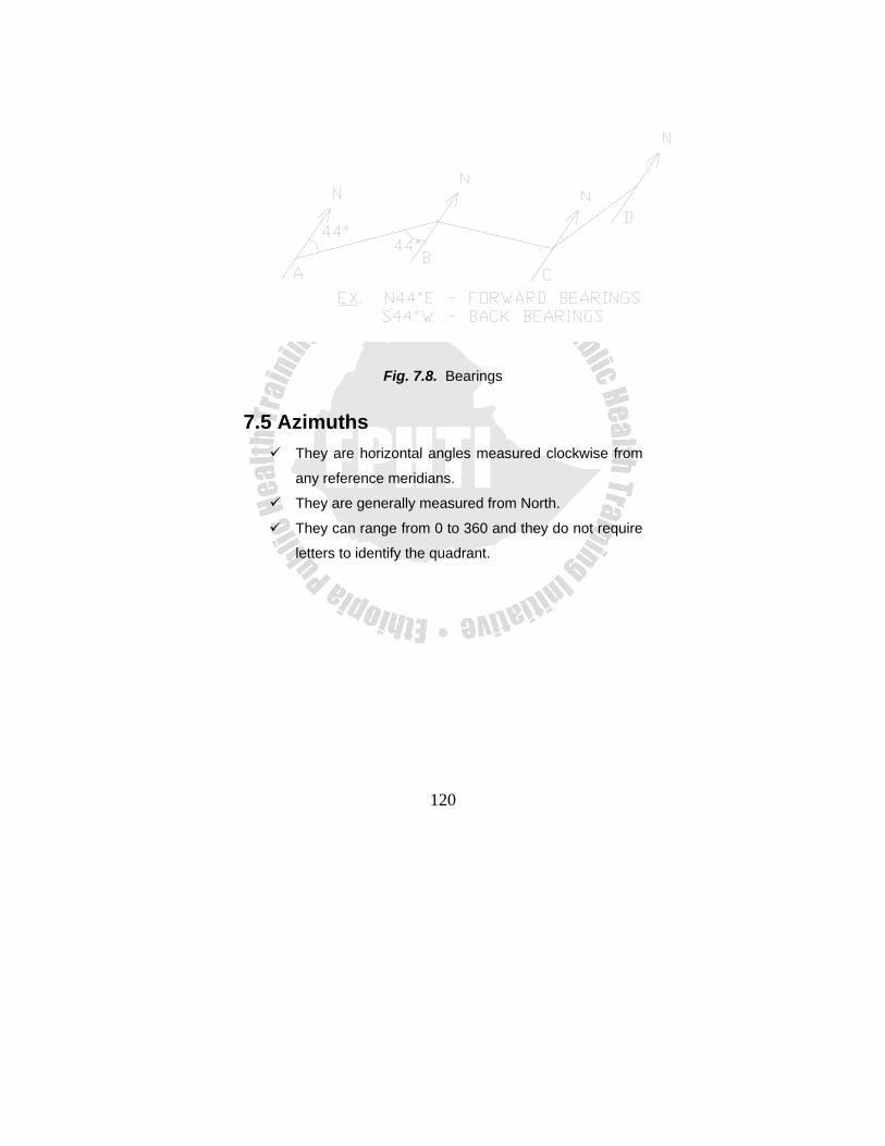
120
Fig. 7.8. Bearings
7.5 Azimuths They are horizontal angles measured clockwise from
any reference meridians.
They are generally measured from North.
They can range from 0 to 360 and they do not require
letters to identify the quadrant.
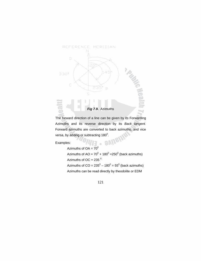
121
Fig 7.9. Azimuths
The forward direction of a line can be given by its Forwarding
Azimuths and its reverse direction by its Back tangent.
Forward azimuths are converted to back azimuths, and vice
versa, by adding or subtracting 1800.
Examples:
Azimuths of OA = 700
Azimuths of AO = 700 + 1800 =2500 (back azimuths)
Azimuths of OC = 235 0
Azimuths of CO = 2350 – 1800 = 550 (back azimuths)
Azimuths can be read directly by theodolite or EDM
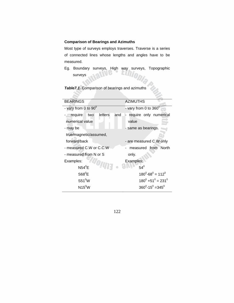
122
Comparison of Bearings and Azimuths Most type of surveys employs traverses. Traverse is a series
of connected lines whose lengths and angles have to be
measured.
Eg. Boundary surveys, High way surveys, Topographic
surveys
Table7.1. Comparison of bearings and azimuths
BEARINGS AZIMUTHS
- vary from 0 to 900
- require two letters and
numerical value
- may be
true/magnetic/assumed,
forward/back
- measured C.W or C.C.W
- measured from N or S
Examples:
N540E
S680E
S510W
N150W
- vary from 0 to 3600
- require only numerical
value
- same as bearings.
- are measured C.W only
- measured from North
only.
Examples:
540
1800-680 = 1120
1800 +510 = 2310
3600-150 =3450
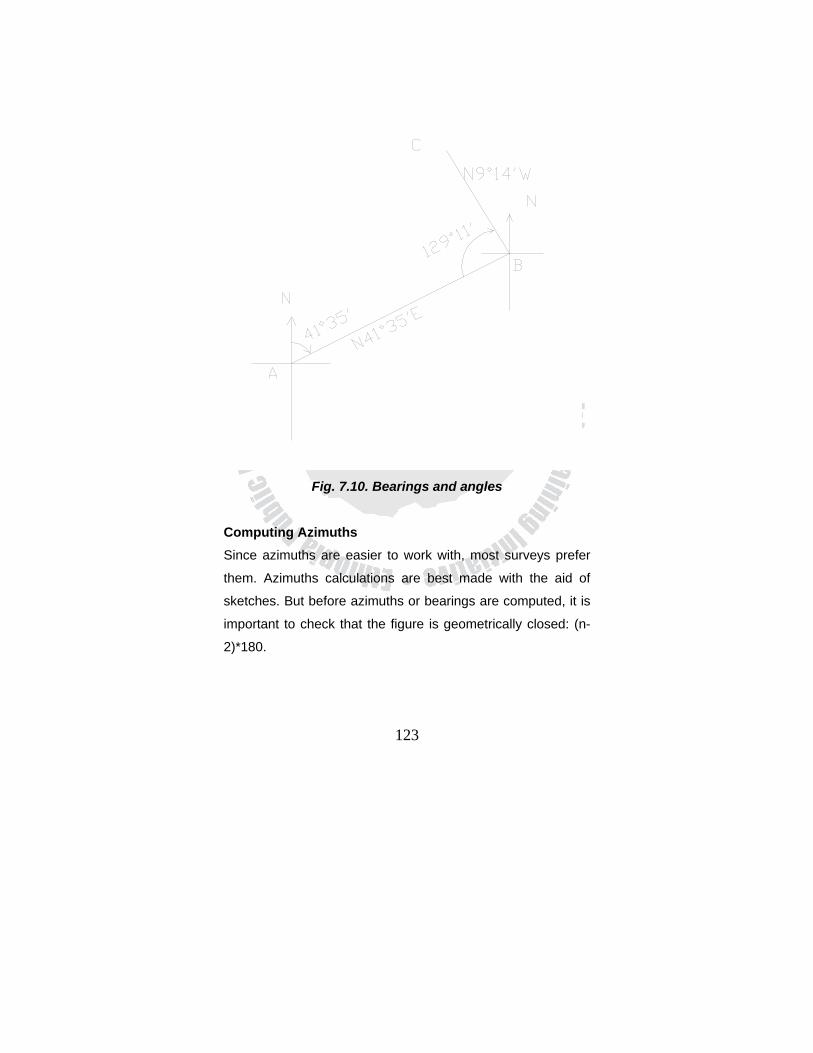
123
Fig. 7.10. Bearings and angles
Computing Azimuths Since azimuths are easier to work with, most surveys prefer
them. Azimuths calculations are best made with the aid of
sketches. But before azimuths or bearings are computed, it is
important to check that the figure is geometrically closed: (n-
2)*180.
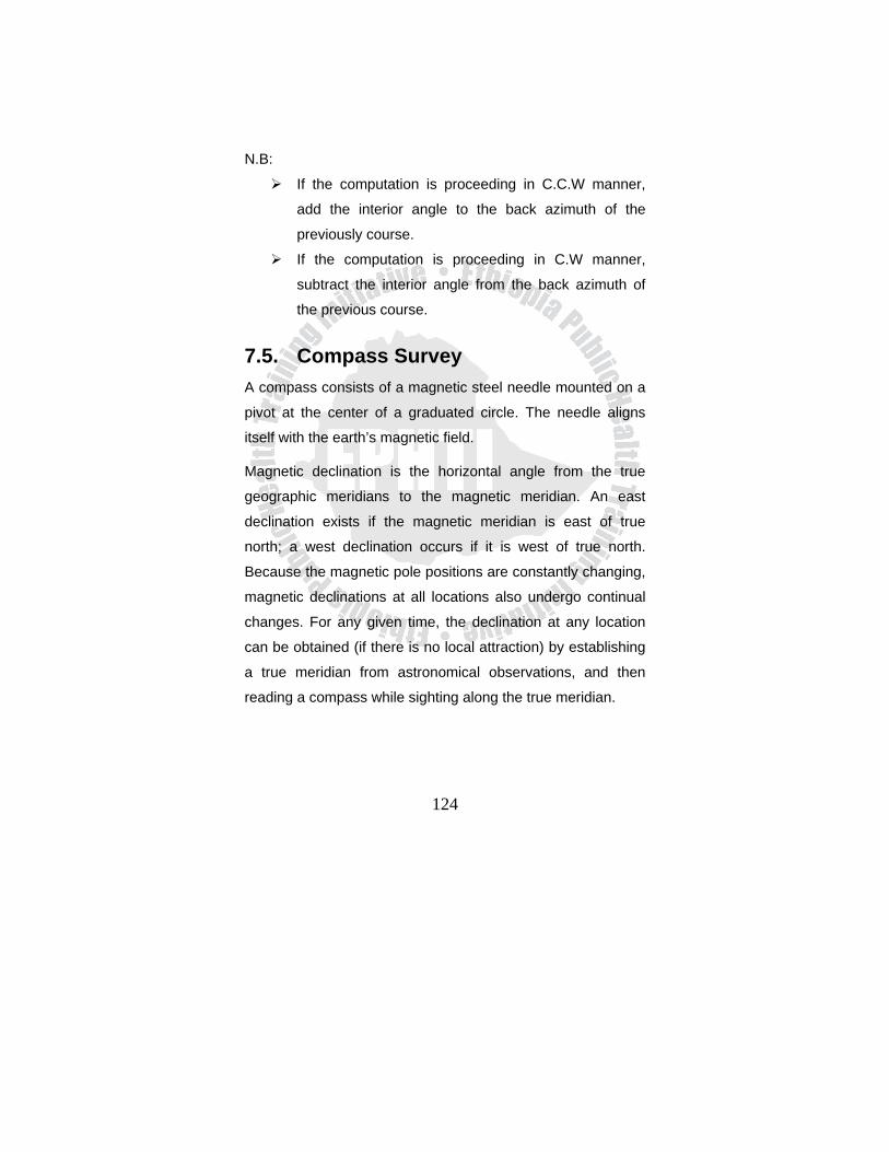
124
N.B:
If the computation is proceeding in C.C.W manner,
add the interior angle to the back azimuth of the
previously course.
If the computation is proceeding in C.W manner,
subtract the interior angle from the back azimuth of
the previous course.
7.5. Compass Survey A compass consists of a magnetic steel needle mounted on a
pivot at the center of a graduated circle. The needle aligns
itself with the earth’s magnetic field.
Magnetic declination is the horizontal angle from the true
geographic meridians to the magnetic meridian. An east
declination exists if the magnetic meridian is east of true
north; a west declination occurs if it is west of true north.
Because the magnetic pole positions are constantly changing,
magnetic declinations at all locations also undergo continual
changes. For any given time, the declination at any location
can be obtained (if there is no local attraction) by establishing
a true meridian from astronomical observations, and then
reading a compass while sighting along the true meridian.
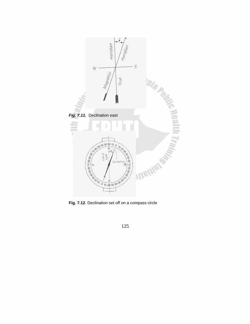
125
Fig. 7.11. Declination east
Fig. 7.12. Declination set off on a compass circle
126
The magnetic field is affected by metallic objects and direct-
current electricity, both of which cause a local attraction. As
an example, when set up besides an old-time street car with
overhead power lines, the compass needle would swing
toward the car as it approached, then follow it until it was out
of an effective range.
If the source of an artificial disturbance is fixed, all bearings
from a given station will be in error by the same amount.
Angles calculated from bearings taken at station will be
correct, however. Local attraction is present if the forward and
back bearings of a line differ by more than the normal
observation errors. Consider the following compass bearings
read on a series of lines:
AB…………………………N24015’W
BA…………………………S24010’E
CD…………………………N60000’E
DC………………………….S61015’W
Forward bearing AB and back bearing BA agree reasonably
well, indicating that little or no local attraction exists at A or B.
However, the bearings at D differ from corresponding
bearings taken at C by roughly 1015’ to the west of north.
Local attraction therefore exists at point D and deflects the
compass needle approximately 1015’ to the west of north.

127
It is evident that to detect local attractions, successive stations
on a compass traverse have to be occupied and forward and
back bearings read, even though the directions of all lines
could be determined by setting up an instrument only on
alternate stations.
128
Exercise 1. The following azimuths are from the north; 329020’,
180035’, 48032’, 170030’, 145025’. Express theses
directions as
a. Azimuths from the south
b. Back azimuths
c. Bearings
2. The following are bearings: S21025’W, N88042’W,
N69052’E, S42025’E. Express theses directions as:
a. Azimuths from north
b. Back azimuths
3. The following azimuths are reckoned from the north. FE =
4025’, ED = 90015’, DC = 271032’, CD = 320021’ and BA =
190045’. What are the corresponding bearings? What are
the deflection angles between consecutive lines?
4. The interior angles of a five-sided closed polygon ABCDE
are as follows. A = 120024’, B = 80015’, C = 132024’, D =
142020’. The angle at E is not measured. Compute the
angle at E, assuming the given values to be correct.
129
5. The magnetic bearings of a line is S47030’E and the
magnetic declination is 8020’E. What is the true bearing of
the line?
6. In an old survey made when the declination was 4015’E,
the magnetic bearing of a given line was N35015’E. The
declination in the same locality now is 1010’W. What are
the true bearings and the present magnetic bearing that
would be used in retracing the line?

130
CHAPTER EIGHT TRAVERSING
8.1. Learning Objectives At the end of this chapter, the student will be able to:
1. Define and identify open and closed traversing
2. Mention and describe the general steps of traverse
computation
3. Define the importance of traverse computation in omitted
measurement
4. Compute area of plots by using different types of area
computation techniques
8.2. Introduction A traverse consists of an interconnected series of lines, called
courses, running between a series of points on the ground,
called traverse stations. A traverse survey is performed in
order to measure both the distances between the stations and
the angles between the courses.
Traverse is generally a control survey and is employed in all
forms of legal and engineering works. It is a series of
established stations that are tied together by angle and
distance.
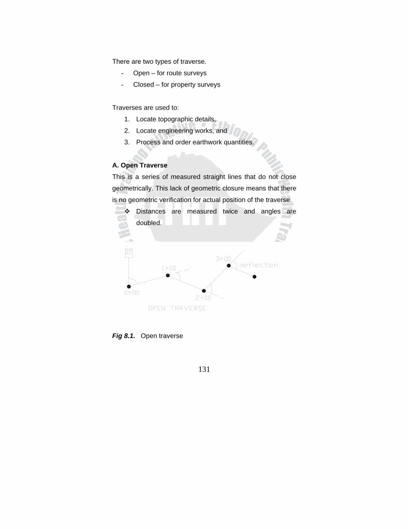
131
There are two types of traverse.
- Open – for route surveys
- Closed – for property surveys
Traverses are used to:
1. Locate topographic details,
2. Locate engineering works, and
3. Process and order earthwork quantities.
A. Open Traverse This is a series of measured straight lines that do not close
geometrically. This lack of geometric closure means that there
is no geometric verification for actual position of the traverse.
Distances are measured twice and angles are
doubled.
Fig 8.1. Open traverse
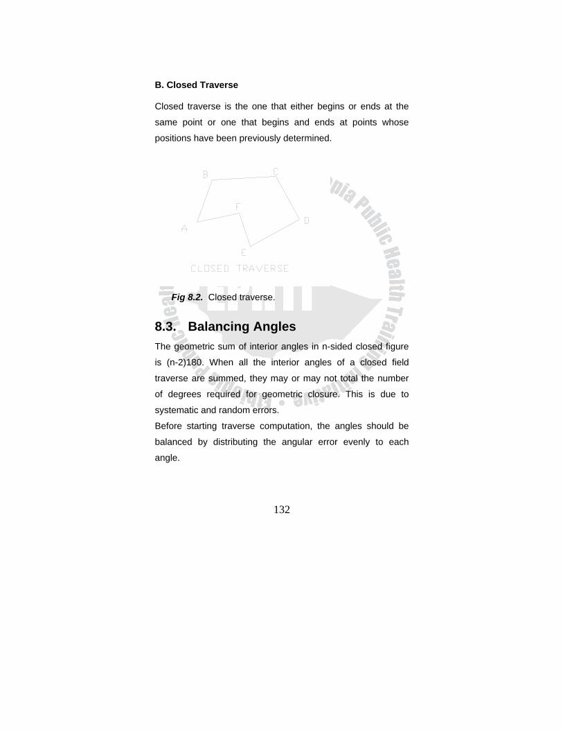
132
B. Closed Traverse
Closed traverse is the one that either begins or ends at the
same point or one that begins and ends at points whose
positions have been previously determined.
Fig 8.2. Closed traverse.
8.3. Balancing Angles The geometric sum of interior angles in n-sided closed figure
is (n-2)180. When all the interior angles of a closed field
traverse are summed, they may or may not total the number
of degrees required for geometric closure. This is due to
systematic and random errors.
Before starting traverse computation, the angles should be
balanced by distributing the angular error evenly to each
angle.
133
The acceptable total error of angular closure is usually quite
small (<03’); otherwise the fieldwork will have to be repeated.
8.4 Latitudes and Departures
We know that a point could be located by either polar co-
ordinate or rectangular co-ordinate system. By definition,
latitude is the north/south rectangular component of a line,
and to differentiate directions, north is considered plus,
whereas south minus. Similarly departure is the east /west
rectangular component of a line.
When working with azimuths:
Latitude (ΔY) =distance (H) cosα
Departure (ΔX) = distance (H) sinα
Where:
α is the bearing or azimuths of the traverse course, and
distance (H) is the horizontal distance of the traverse
course.
Latitudes (lats) and departures (deps) can be used to
calculate the accuracy of a traverse by noting the plus/minus
course of both lats and deps. If the survey has been
performed, the plus latitudes will equal the minus latitudes,
and the plus departures will equal the minus departures.
134
N.B: For azimuths directions the algebraic sign of the
appropriate trigonometric functions governs the
algebraic sign.
Computation of Latitudes and Departures to Determine the Error of Closure and the Precision of a Traverse
In the computation of latitudes and departures, the following
steps should be followed.
1. Balance the angles.
2. Compute the bearings (azimuths).
3. Compute the latitudes(Δy) and departures(Δx).
For example, if the traverse computation begins at A and is
concluded at A’, the error of closure is given by the line A’ A,
and the correction of latitude (Clat) and the correction of
departure (Cdep) are in fact the latitudes and departures of
the linear error of closure.
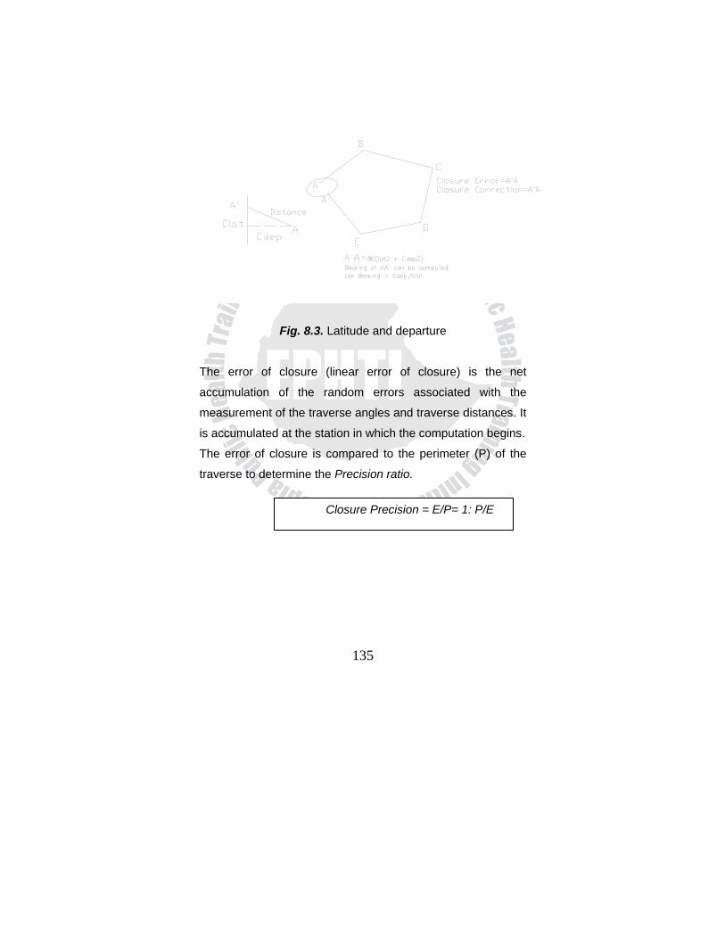
135
Fig. 8.3. Latitude and departure
The error of closure (linear error of closure) is the net
accumulation of the random errors associated with the
measurement of the traverse angles and traverse distances. It
is accumulated at the station in which the computation begins.
The error of closure is compared to the perimeter (P) of the
traverse to determine the Precision ratio.
Closure Precision = E/P= 1: P/E
136
8.5. Traverse Adjustment
Latitudes and departures can be used for the computations of
co-ordinates or the computation of the area of enclosed by the
traverse. However, before any further use can be made of
these latitudes and departures, they must be adjusted so that
their errors are suitably distributed, and the algebraic sums of
the latitudes and departures are each zero.
There are two ways of traverse adjustment:
1. Compass (Bow ditch) rule-the common way
2. Transit rule: this is a complicated and lengthy
procedure when done manually. It is now being
applied by surveyors with increasing frequency when
canned computer programs are used to adjust and
close the traverse.
Compass Rule
It Is Used In Many Survey Computations To Distribute The
Errors In Latitudes And Departures. The Compass Rule
Distributes The Errors In Latitudes And Departures For Each
Traverse Course In The Same Proportion As The Course
Distance Is To The Perimeter.
OR
Clat AB = AB ∑lat P
Clat AB =∑ lat X AB P
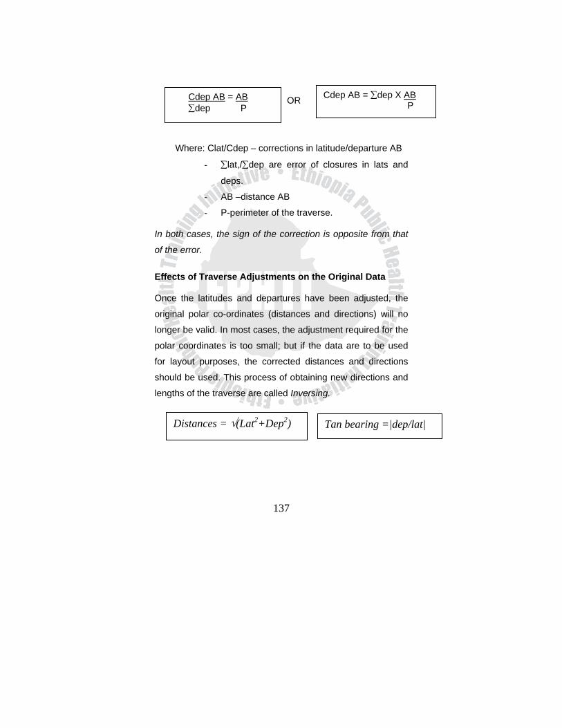
137
OR
Where: Clat/Cdep – corrections in latitude/departure AB
- ∑lat,/∑dep are error of closures in lats and
deps.
- AB –distance AB
- P-perimeter of the traverse.
In both cases, the sign of the correction is opposite from that
of the error.
Effects of Traverse Adjustments on the Original Data
Once the latitudes and departures have been adjusted, the
original polar co-ordinates (distances and directions) will no
longer be valid. In most cases, the adjustment required for the
polar coordinates is too small; but if the data are to be used
for layout purposes, the corrected distances and directions
should be used. This process of obtaining new directions and
lengths of the traverse are called Inversing.
Cdep AB = AB ∑dep P
Cdep AB = ∑dep X AB P
Distances = √(Lat2+Dep2) Tan bearing =|dep/lat|
138
Computation of Coordinates The relative positions of control stations are best defined by
their rectangular or XY coordinates.
Their rectangular coordinates best define the relative positions
of control stations. In most surveying applications, the Y
(north) coordinates precedes the X (east) coordinates.
Coordinates of a point may be computed by successive
algebraic addition of the adjusted latitudes and departures to
the assumed N and E co-ordinates respectively.
Where: N2 and E2 are the Y and X co-ordinates of station 2
N1 and E1 are the Y and X co-ordinates of station1
Lat1-2 = the latitudes of course 1-2
Dep1-2 = the departure of course 1-2
8.6 Application of Traversing
8.6.1. Omitted Measurements The techniques developed in the computation of latitudes and
departures can be used to supply missing course information
on a closed traverse and can be used to solve any problem
that can be arranged in the form of a closed traverse.
N2 = N1 + Lat1-2 E2 = E1 +Dep1-2
139
The data can be treated in the same manner as in a closed
traverse. When the latitudes and departures are totaled, they
will not balance. Both the latitudes and departures will fail to
close by the missing course.
8.6.2. Area Of A Closed Traverse
BY THE COORDINATE METHOD
When the coordinates of the stations of a closed traverse are
known, it is simple matter to compute the area with in the
traverse.
By definition,” the double area of a closed traverse is the
algebraic sum of each X co-ordinates multiplied by the
difference between the Y values of the adjacent stations.”
The double area is divided by 2 to determine the final area.
The final area can be positive or negative, reflecting only the
direction of computation approach (C.W or C.C.W). But the
area is always positive.
Distance = √(Lat2+Dep2) Tan bearing = |dep/lat|
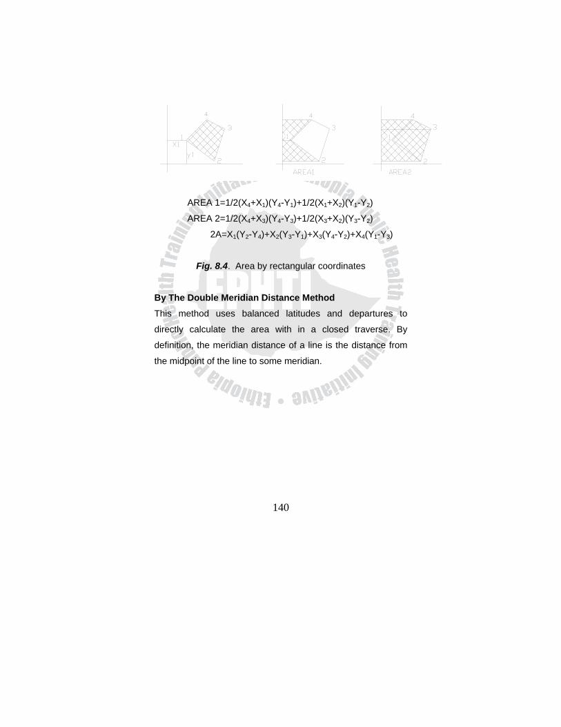
140
AREA 1=1/2(X4+X1)(Y4-Y1)+1/2(X1+X2)(Y1-Y2)
AREA 2=1/2(X4+X3)(Y4-Y3)+1/2(X3+X2)(Y3-Y2)
2A=X1(Y2-Y4)+X2(Y3-Y1)+X3(Y4-Y2)+X4(Y1-Y3)
Fig. 8.4. Area by rectangular coordinates
By The Double Meridian Distance Method This method uses balanced latitudes and departures to
directly calculate the area with in a closed traverse. By
definition, the meridian distance of a line is the distance from
the midpoint of the line to some meridian.
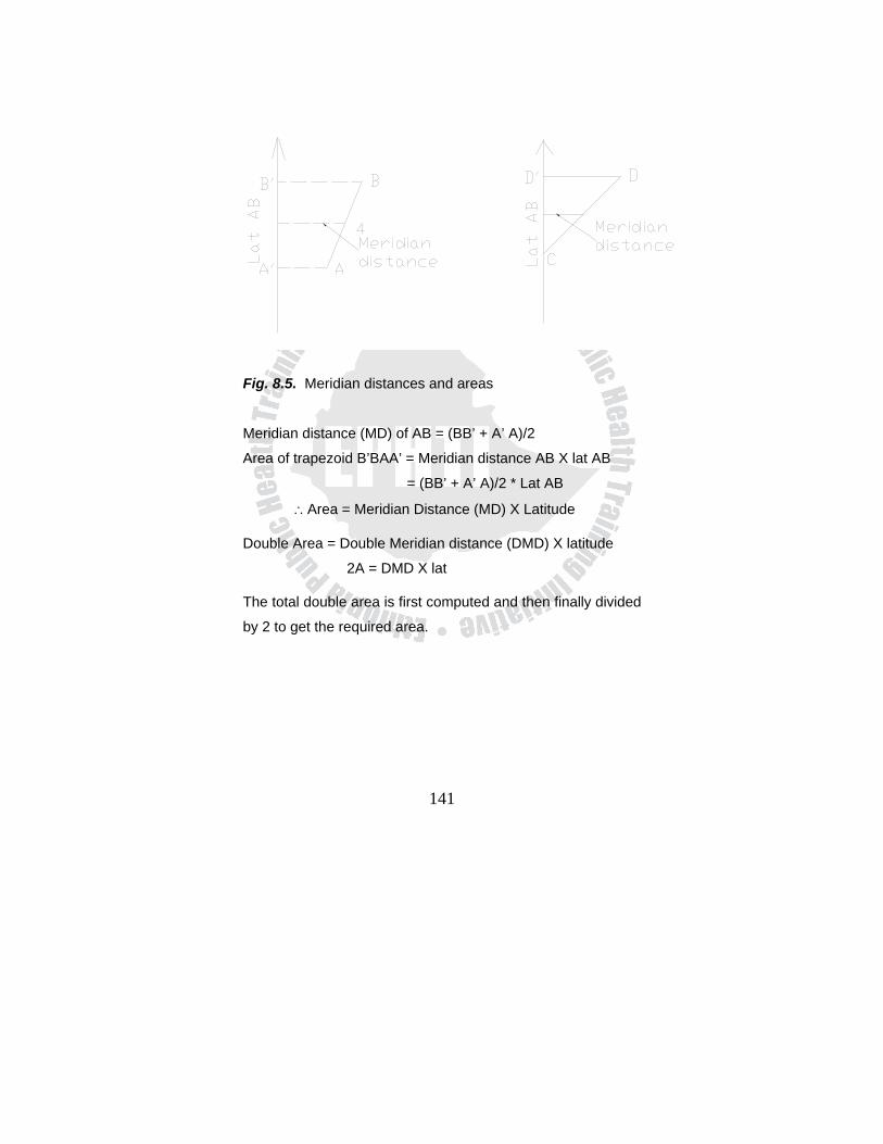
141
Fig. 8.5. Meridian distances and areas
Meridian distance (MD) of AB = (BB’ + A’ A)/2
Area of trapezoid B’BAA’ = Meridian distance AB X lat AB
= (BB’ + A’ A)/2 * Lat AB
∴Area = Meridian Distance (MD) X Latitude
Double Area = Double Meridian distance (DMD) X latitude
2A = DMD X lat
The total double area is first computed and then finally divided
by 2 to get the required area.
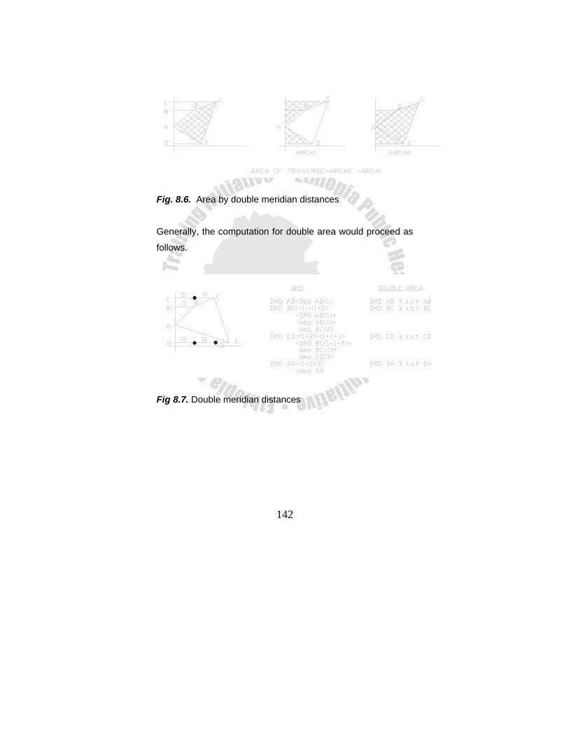
142
Fig. 8.6. Area by double meridian distances
Generally, the computation for double area would proceed as
follows.
Fig 8.7. Double meridian distances

143
N.B The DMD of the first course is equal to the departure
of the first course.
The DMD of each succeeding course is equal to the
DMD of the previous course + the departure of the
previous course + the departure of the course itself.
The DMD of the last course will turn out to be equal to
the departure of the last course, but opposite in sign.
Summary of Traverse Computations 1. Balance the field angles
2. Correct (if necessary) the field distance (e.g. for
temperature, sag)
3. Compute the bearings or azimuths
4. Compute the linear error of closure and the accuracy
ratio of the traverse
5. Compute the balanced latitudes and balanced
departures
6. Compute the coordinates
7. Compute the area by coordinate or by DMDs method
144
8.6.3 Mistakes in Traverse Computations
Some of the common mistakes made in traverse
computations are:
1. Failing to adjust the angles before computing azimuths
or bearings
2. Applying angle adjustment in the wrong direction and
failing to check the angle sum for proper geometric total
3. Interchanging departures and latitudes, or their signs
4. Confusing the signs of coordinates
5. Carrying out corrections beyond the number of decimal
places in the original measurements
145
Exercise 1. A five-sided closed field traverse have the following
angles. A = 103003’30”, B = 113044’00”, C = 88021’30”, D
= 110053’30”, E = 123055’00”. Determine the angular error
of closure and balance the angles by applying equal
correction to each angle.
2. A four-sided closed field traverse has the following
angles. A = 81022’30”, B = 72032’30”, C = 89039’30”, D =
116023’30”. The length of the sides are as follows: AB =
636.45ft, BC = 654.49ft, CD = 382.85ft, DA = 512.77ft.
The bearing of AB is 533019’W, BC is in the SE quadrant.
a) Balance the field angles
b) Compute the bearing or the azimuth
c) Compute the latitude and departures
d) Determine the linear error of closure and the
accuracy ratio
e) Balance the latitudes and departures by using
the Compass rule.
f) Compute the coordinates of station A, C and D
if the coordinate of station B are 1000.00N,
1000.00E
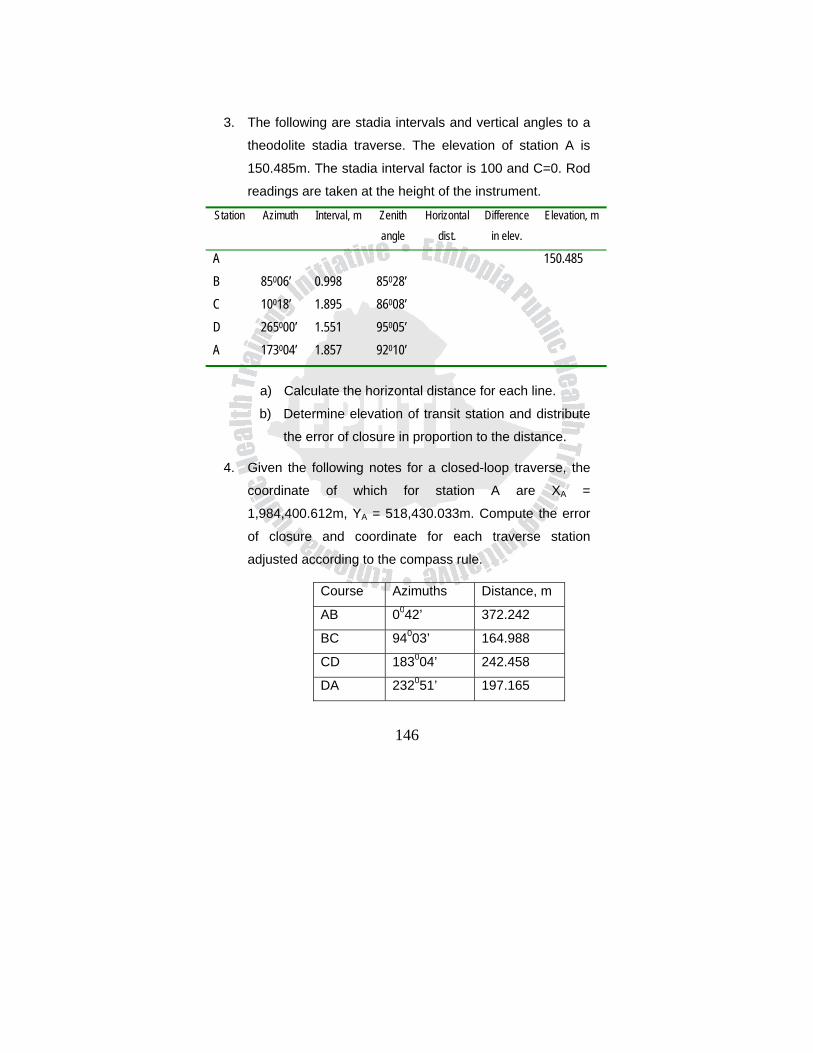
146
3. The following are stadia intervals and vertical angles to a
theodolite stadia traverse. The elevation of station A is
150.485m. The stadia interval factor is 100 and C=0. Rod
readings are taken at the height of the instrument.
Station Azimuth Interval, m Zenith angle
Horizontal dist.
Difference in elev.
Elevation, m
A 150.485 B 85006’ 0.998 85028’ C 10018’ 1.895 86008’ D 265000’ 1.551 95005’ A 173004’ 1.857 92010’
a) Calculate the horizontal distance for each line.
b) Determine elevation of transit station and distribute
the error of closure in proportion to the distance.
4. Given the following notes for a closed-loop traverse, the
coordinate of which for station A are XA =
1,984,400.612m, YA = 518,430.033m. Compute the error
of closure and coordinate for each traverse station
adjusted according to the compass rule.
Course Azimuths Distance, m
AB 0042’ 372.242
BC 94003’ 164.988
CD 183004’ 242.458
DA 232051’ 197.165
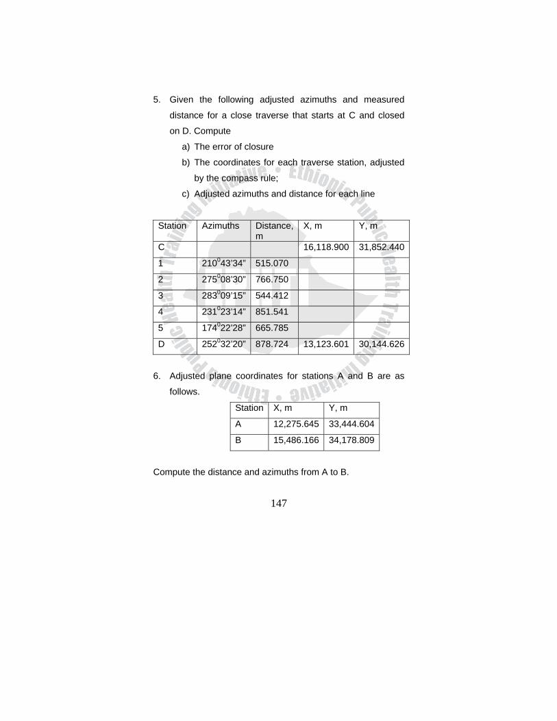
147
5. Given the following adjusted azimuths and measured
distance for a close traverse that starts at C and closed
on D. Compute
a) The error of closure
b) The coordinates for each traverse station, adjusted
by the compass rule;
c) Adjusted azimuths and distance for each line
Station Azimuths Distance, m
X, m Y, m
C 16,118.900 31,852.440
1 210043’34” 515.070
2 275008’30” 766.750
3 283009’15” 544.412
4 231023’14” 851.541
5 174022’28” 665.785
D 252032’20” 878.724 13,123.601 30,144.626
6. Adjusted plane coordinates for stations A and B are as
follows.
Station X, m Y, m
A 12,275.645 33,444.604
B 15,486.166 34,178.809
Compute the distance and azimuths from A to B.
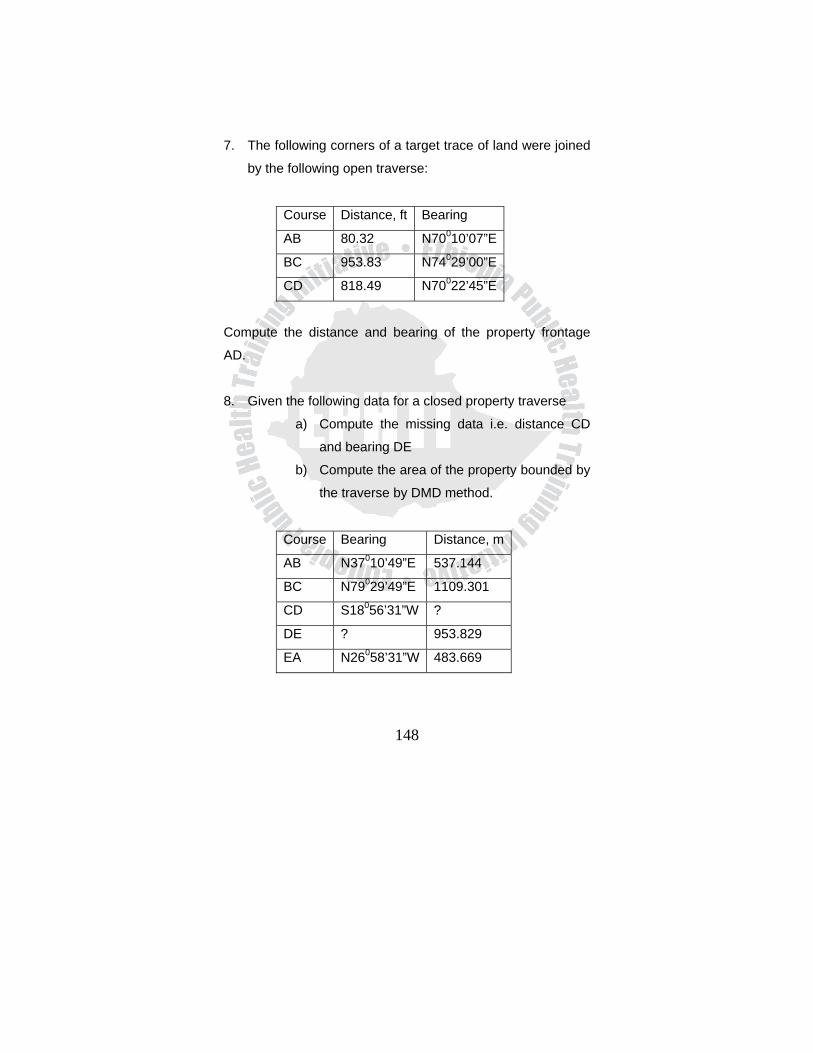
148
7. The following corners of a target trace of land were joined
by the following open traverse:
Course Distance, ft Bearing
AB 80.32 N70010’07”E
BC 953.83 N74029’00”E
CD 818.49 N70022’45”E
Compute the distance and bearing of the property frontage
AD.
8. Given the following data for a closed property traverse
a) Compute the missing data i.e. distance CD
and bearing DE
b) Compute the area of the property bounded by
the traverse by DMD method.
Course Bearing Distance, m
AB N37010’49”E 537.144
BC N79029’49”E 1109.301
CD S18056’31”W ?
DE ? 953.829
EA N26058’31”W 483.669

149
9. The following table gives X and Y coordinates (in meter)
for stations in a closed traverse. Calculate the area
enclosed by the traverse using the coordinate method.
Coordinates Stations
A B C D
X 4000 4100.5 4205.7 4103.4
Y 4000 4150.3 4875.0 4870.6
10. The following table gives the departure and latitudes of
an adjusted closed traverse. Calculate the area by DMD
method.
Course Departures, m Latitudes, m
+ - + -
AB 313.6 198.7
BC 274.4 281.1
CD 189.2 134.1
DE 110.7 324.9
EA 288.1 541.4
150
CHAPTER NINE CONSTRUCTION SURVEYS
9.1 Learning Objectives
At the end of this chapter, the student will be able to:
1. Describe the different types of construction surveys
2. Develop skills for construction of sewer and other
constructions.
9.2. Introduction
Construction surveys provide the horizontal and vertical layout
for every key component of a construction project. This
provision of line and grade can only be accomplished by
experienced surveyors familiar with both the related project
design and the appropriate construction techniques. A
knowledge of related design is essential to interpret the
design drawings effectively for layout purposes, and a
knowledge of construction techniques is required to ensure
that the lay out is optimal for both line and grade transfer and
construction schedule.
On any construction site, it is general practice to construct
firstly the roadways and sewers, in order to provide a) access
to the site and b) main drainage to all buildings.
151
All roads, buildings, drains and sewers are set out using
standard surveying equipment comprising:
1. Steel tapes: it must always be used for setting out
purposes as they are not subject to the same degree of
stretching as are Fibron tapes. The accuracy of setting
out work is largely dependent up on the condition of the
tape and or course, the expertise of the user.
2. Levels: automatic levels are used on most sites. They
compare favorably in price with optical levels and produce
much more reliable results.
3. Theodolites: a wide variety of theodolite is now available
but, as with levels, the more automation that can be
provided, the greater will be the accuracy of the setting
out. Thus, it is a good practice to use theodolite with
optical plumbing, automatic vertical circle indexing,
electronic readout and electronic two axis leveling.
4. Total station: most setting out work, particularly road
ways, can be readily and accurately accomplished by the
method of coordinates. An EDM instrument is required to
set the distances and total stations can set out horizontal
distances with ease.
152
5. Autoplumb instruments: These instruments are used to
set a vertical line in high-rise buildings. They are much
more convenient to use this purpose than theodolites.
They save much time and greatly increase accuracy.
6. Pegs: these are either wooden 50mm X 50mm X 500mm
stakes for use in soft ground or 25mm X 25mm X 300mm
angle irons for hard standing.
7. Profiles: is a wooden stake to which a cross-piece,
painted in contrasting coloured stripes, is nailed. For
sewer work, goalpost-type profiles, called sight rails, are
preferable. The profiles are elected over the offset pegs in
order to remain clear of the excavation.
8. Travelers: are really mobile profile boards used in
conjunction with sight rails. The length of the traveler
equals the sight rail level- sewer invert level. The length of
0.25 meters and travelers are usually about 2 meters
long.
9. Corner profiles: during the construction of buildings, the
pegs denoting the corners of the buildings are always
removed during the construction work. The corner
positions have, therefore, to be removed some distance
back from the excavations on to corner profiles. These
are constructed from stout wooden stakes 50mm X
50mm, on to which wooden boards 250mm X 25mm X
1.00m long are securely nailed.
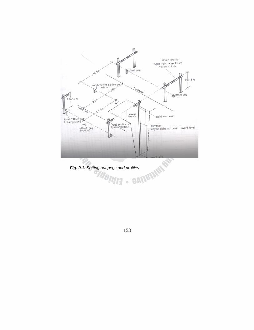
153
Fig. 9.1. Setting out pegs and profiles
154
9.3. Setting out a Peg on a Specified Distance and Bearing
A. Setting Out On Level Ground
In order to set out the roads, buildings and sewers shown on
the development plan, a total of some forty to fifty pegs need
to be accurately placed on the ground in their proposed
positions. Fortunately, every peg is set out in exactly the same
manner. It is not an easy task to physically set a peg in its
exact proposed location and, in order to do so, the following
sequence of operations is required.
In figure 9.2a, a peg C is to be set out from a survey line AB.
A surveyor and two assistants are usually required to
complete the task.
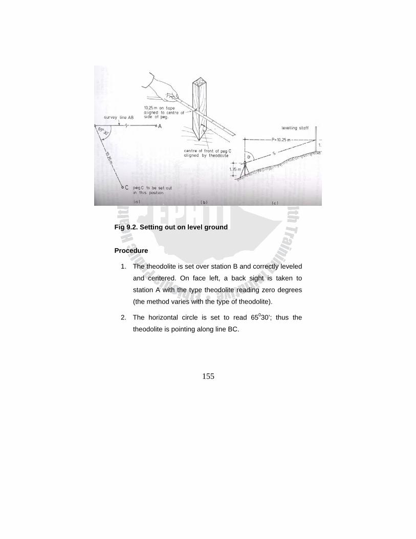
155
Fig 9.2. Setting out on level ground Procedure
1. The theodolite is set over station B and correctly leveled
and centered. On face left, a back sight is taken to
station A with the type theodolite reading zero degrees
(the method varies with the type of theodolite).
2. The horizontal circle is set to read 65030’; thus the
theodolite is pointing along line BC.
156
3. The end of the tape is held against the nail in peg B and
laid out approximately along the line BC by the
assistants.
4. The 10.25 m reading on the tape is held against the
SIDE of the proposed peg C(In figure 9.2b), the tape is
tightened and slowly swing in an arc, until the surveyor
sees it clearly through the telescope of the theodolite.
5. The peg is carefully moved, on the observer’s
instructions, until the bottom, front edge of the peg is
accurately bisected. The peg is then hammered home.
6. The tape is again held at peg B, by assistant 1, while
assistant 2 tightens it and marks a pencil line across the
peg C at distance 10.25 m.
7. A pencil is held vertically on this line by an assistant and
is moved slowly along the line until the surveyor sees it
bisected by the line of sight through the theodolite. The
assistant marks this point on the peg.
8. The distance of 10.25 m is checked and the operation is
repeated on face right. If all is well, the two positions of
point C should coincide or differ by a very few
millimeters. The mean is accepted and a nail
hammered into the peg to denote point C.
157
It is not good practice to hook the end of the tape over the nail
at peg B when setting out the distance, as excessive tension
on the tape will move the nail head or even move the peg.
B. Setting Out On Sloping Ground In all setting out operations, the horizontal distance is
required, but frequently, because of ground undulations, it will
be necessary to set out the slope distance. The setting-out
procedure is very similar to that of setting out on a level
ground.
1. The theodolite is set up at station B, back sighted to A
reading zero and foresighted along the line BC reading
65030’. The instrument height is measured and noted. Let
the height be 1.35 m.
2. The tape is stretched out in the proposed direction of line
BC and a leveling staff held vertically at distance 10.25 m.
3. The instrument height (1.35 m) is read on the staff and
the angle of inclination (vertical or zenith angle) is noted.
Let the zenith angle be 84o 15’.
4. The distance to be set out on the slope will have to be
increased to be the equivalent of 10.25 m of plan length,
as follows (Figure 9.2c):
158
Plan length (p) /slope length (S)
= sin zenith angle
Slope length S = plan length p / sin zenith angle
S = 10.250/sin 840 15’
= 10.302 m
5. The procedure in setting out peg C then follows exactly
the procedure detailed in out on a level ground, using the
new setting out length of 10.302 m.
9.4. Setting Out Small Buildings
Dwelling houses are still largely traditionally built and small
inaccuracies in the setting out can usually be tolerated. Large
factory buildings, multi-storey buildings, schools, etc., are
nowadays largely prefabricated and little, if any, inaccuracy
can be tolerated in the setting out. Consequently the methods
of setting out vary considerably.
The exact position that the building is to occupy on the ground
is governed by the building line as defined by the local
authority.
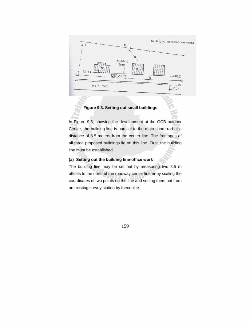
159
Figure 9.3. Setting out small buildings
In Figure 9.3, showing the development at the GCB outdoor
Center, the building line is parallel to the main shore rod at a
distance of 8.5 meters from the center line. The frontages of
all three proposed buildings lie on this line. First, the building
line must be established.
(a) Setting out the building line-office work The building line may be set out by measuring two 8.5 m
offsets to the north of the roadway center line or by scaling the
coordinates of two points on the line and setting them out from
an existing survey station by theodolite.
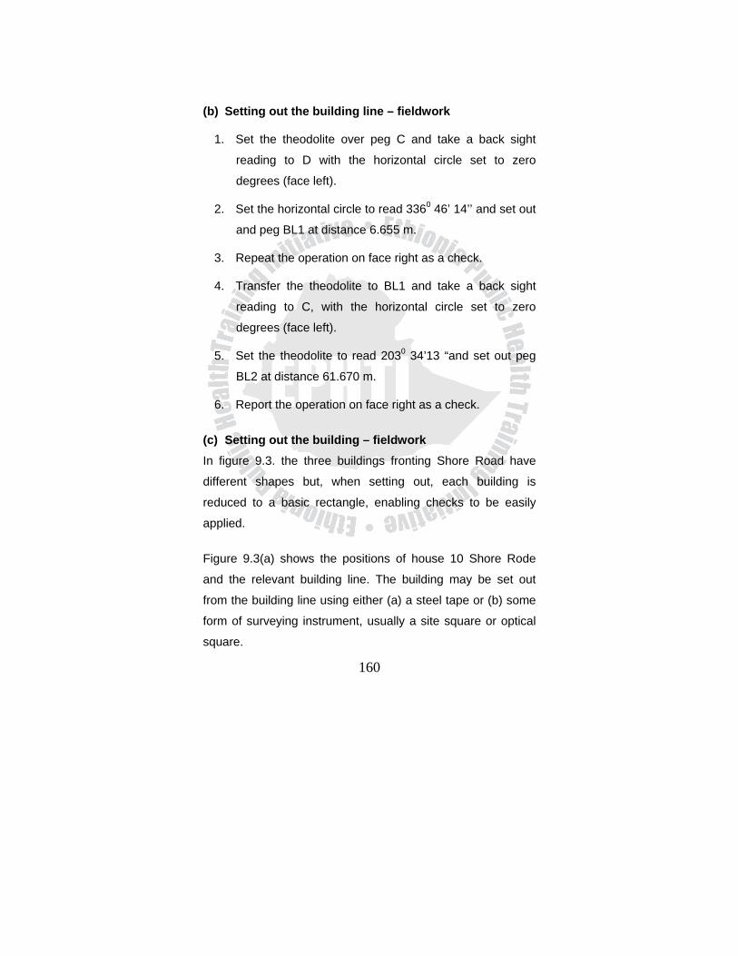
160
(b) Setting out the building line – fieldwork
1. Set the theodolite over peg C and take a back sight
reading to D with the horizontal circle set to zero
degrees (face left).
2. Set the horizontal circle to read 3360 46’ 14’’ and set out
and peg BL1 at distance 6.655 m.
3. Repeat the operation on face right as a check.
4. Transfer the theodolite to BL1 and take a back sight
reading to C, with the horizontal circle set to zero
degrees (face left).
5. Set the theodolite to read 2030 34’13 “and set out peg
BL2 at distance 61.670 m.
6. Report the operation on face right as a check.
(c) Setting out the building – fieldwork
In figure 9.3. the three buildings fronting Shore Road have
different shapes but, when setting out, each building is
reduced to a basic rectangle, enabling checks to be easily
applied.
Figure 9.3(a) shows the positions of house 10 Shore Rode
and the relevant building line. The building may be set out
from the building line using either (a) a steel tape or (b) some
form of surveying instrument, usually a site square or optical
square.
161
Procedure
1. Using a scale rule, measure on the plan the distance
between the building line starting point BL1 and the
corner A of the house. The scaled dimension is 2.50 m.
2. Determine, from the plan, the dimensions of a basic
rectangle to enclose the house. The scaled dimensions
are 13.0 m by 8.0 m.
3. Using a steel tape set out the distance 2.50 m along the
building line from point BL1, to establish corner A of the
house. Mark the point by a nail driven into a wooden peg.
4. Measure the distance AB (13.0 m) along the building line
and establish a peg at B. Mark the point by a nail.
5. Using a basic 3:4:5 right angle, measure the lengths AD
and BC (8.0 m) and establish pegs at C and D.
6. Check the length of the diagonals AC and BD (15.264 m).
Both measurements should be equal, thus providing that
the building is square.
Although the method of setting out a right angle using a 3:4:5
triangle is theoretically sound, in practice it tends to lead to
inaccuracy in positioning. By calculating the length of diagonal
of the rectangle and using two tapes, the setting out can be
accomplished.
162
Figure 9.4. Setting out the building
Setting Out On Sloping Ground
When setting out buildings on sloping ground, it must be
remembered that the dimensions taken from the plan are
horizontal lengths and consequently the tape must be held
horizontally and the method of step taping used.
The diagonals must also be measured horizontally and in
practice considerable difficulty is experienced in obtaining
checks under such conditions. Besides, the method is
laborious and time consuming.
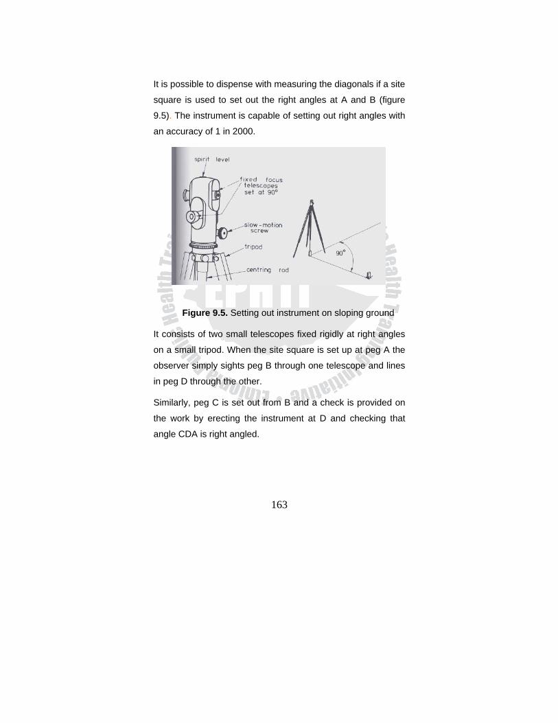
163
It is possible to dispense with measuring the diagonals if a site
square is used to set out the right angles at A and B (figure
9.5). The instrument is capable of setting out right angles with
an accuracy of 1 in 2000.
Figure 9.5. Setting out instrument on sloping ground
It consists of two small telescopes fixed rigidly at right angles
on a small tripod. When the site square is set up at peg A the
observer simply sights peg B through one telescope and lines
in peg D through the other.
Similarly, peg C is set out from B and a check is provided on
the work by erecting the instrument at D and checking that
angle CDA is right angled.
164
• Setting out – vertical control
Whenever any proposed level is to be set out, sight rails
(profiles) must be erected either at the proposed level in the
case of a floor level or at some convenient height above the
proposed level in case of foundation levels, formation levels
and invert levels. Suitable forms of sight rails or profiles are
shown in Fig 9.1. The rails should be set at right angles to the
centre lines of drains, sewers, etc.
A traveler or boning rod is a mobile profile which is used in
conjunction with sight rails. The length of the traveler is equal
to the difference in height between the rail level and the
proposed excavation level. Figure 9.1 shows the traveler in
use in a trench excavation.
• Setting out peg at a predetermined level
The basic principle of setting out a profile board at a
predetermined level is shown in figure 9.6.
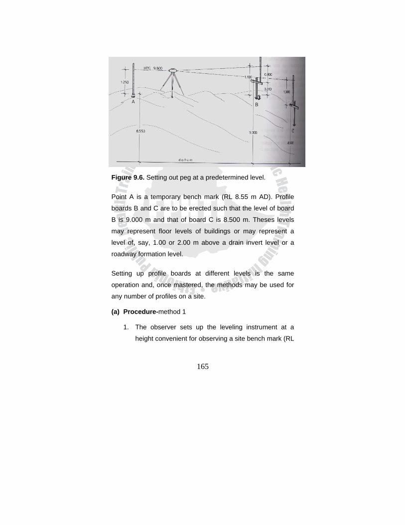
165
Figure 9.6. Setting out peg at a predetermined level.
Point A is a temporary bench mark (RL 8.55 m AD). Profile
boards B and C are to be erected such that the level of board
B is 9.000 m and that of board C is 8.500 m. Theses levels
may represent floor levels of buildings or may represent a
level of, say, 1.00 or 2.00 m above a drain invert level or a
roadway formation level.
Setting up profile boards at different levels is the same
operation and, once mastered, the methods may be used for
any number of profiles on a site.
(a) Procedure-method 1
1. The observer sets up the leveling instrument at a
height convenient for observing a site bench mark (RL

166
8.55 m AD) and takes a back sight staff reading (1.25
m). The height of collimation (HPC) is the therefore
RL Benchmark + BS Reading
i.e. HPC = 8.55 m + m + 1.255 m = 9.80 m.
2. The assistant firmly hammers home a small peg, 300
mm long, besides the profile peg and a fore sight
reading (1.11 m) is taken to a staff held vertically
upon it. The level of the top of the small peg is
therefore
RL = HPC – FS reading
= 9.80 – 1.11 = 8.69 m
3. The difference in level between the top of the small
peg (8.69 m) and the required profile level (9.00 m) is
calculated:
Difference = 9.00 m- 8.69 m = 0.31 m
Using a tape, the assistant measures this height
against the profile peg and marks it in pencil.
4. A profile boars is nailed securely to the profile peg,
such that the upper edge of the board is against the
pencil mark, and is thus at a level of 9.00 m.
This method is widely used on construction sites because of
its simplicity. However, it has the disadvantage that the
observer has to rely upon the assistant (often untrained) to
167
correctly mark the final height on the profile peg. The
disadvantage is overcome by using the following method.
(b) Proceudre-method 2
1. The observer sets up the leveling instrument, takes
a back sight to the benchmark and computes the
height of collimation (HPC) as before;
HPC = RL benchmark + BS reading
= 8.55 m + 1.25 m = 9.80 m
2. The staff man holds the staff against the profile peg
and moves it slowly up or down until the base of the
staff is at a height 9.00 m, exactly. This will occur
when the observer reads 9.80 m – 9.00 m = 0.80 m
on the staff, since
HPC = 9.80 m
Required profile level = 9.00 m
Therefore staff reading = 0.80 m
3. The base of the staff is marked in pencil agasin t
the profile peg and the profile board is nailed
securely to the peg, such that the upper edge of the
board is against the pencil mark.
168
4. Profiel board C is established in exactyu the same
man ner, but since the board is to be erected at
different level, a new calculation is required;
HPC = 9.80 m
Required profile level =8.50 m
Therefore staff reading = (9.80- 8.50) m = 1.30 m
C. The observer sets up the leveling instrument, takes a
back sight to the bench mark and computes the height of
collimation (HPC).
9.5. Sewer and Tunnel Construction Sewers can be categorized in to two broad categories:
1. Sanitary sewers collect residential and industrial liquid
waste and convey these wastes (sewage) to a treatment
pant. 2. Storm sewers are designed to collect runoff from rainfall
and to transport this water (sewage) to the nearest natural
receiving body (e.g. River, lake). The rain water enters the
storm sewer system through ditch inlets or through catch
basins located at the curb line on paved roads.
The design and construction of sanitary and storm sewers are
similar in the respect that the flow of sewage is usually
governed by gravity. Since the sewer grade lines (flow lines)
169
depend on gravity, it is essential that the construction grades
be precisely given.
The sewers usually located 5 feet (1.5m) either side of the
road. The sanitary sewer is usually deeper than the storm
sewer. As it must be deep enough to allow for all house
connections. The sanitary house connection is usually at 2 %
(minimum) slop. If sanitary sewers are being added to an
existing residential road, the preliminary servey must include
the basement floor elevations. The floor elevations are
determined by taking a rod reading on the windowsill and
then, after getting permission to enter the house, measuring
from the windowsill down to the basement floor. As a result of
deep basement s and long setbacks from the main road,
sanitary sewers often have to at least 9 ft (2.75m) below the
main road.
The depth of storm sewers ranges from 3 ft(1m) in some area
of the south to 8 ft 2.5m) in the north. The design of the inlets
and catch basins depends on the depth of sewer and the
quality of the effluent.
The minimum slop for storm sewers is usually 0.50%, where
as the minimum slop for sanitary sewer is often set at 0.67%.
in either case , the designers try to achieve self cleaning
velocity 2.5 to 3 ft per second ( 0.8to 0.9m/s) to avoid
excessive sewer maintenance costs.
170
Manholes (maintenance holes) are located at each change in
direction, slope, or pipe size. In addition, manholes are
located at 300 to 450 ft (100 to 140m) intervals maximum.
Catch basins for storm water are located at 300 ft (100m)
maximum intervals; they are also located at the high side of
intersections and at all low points. The 300 ft (100m)
maximum interval is reduced as the slope on the road
increases.
For construction purpose, sewer layout is considered only
from one man hole to the next. The stationing (0+00)
commences at the first (existing) man hole (or outlet) and
proceeds only to the next man hole. If a second leg is also to
be constructed, that station of 0+00 is assigned to the
downstream manhole and proceeds upstream only to the next
manhole. Each manhole is described by a unique manhole
number to avoid confusion with the stations for extensive
sewer projects.
Tunnel construction Tunnels are used in road, sewer and pipeline construction
when the cost of working at or near the ground surface
becomes productive. For example, sewers are tunneled when
they must be at a depth that would make open cut too
expensive or (operationally unfeasible) , or sewer may be
171
tunneled to avoid disruption of services on the surface such
as would occur if an open cut was put through a busy
expressway. Roads and railroads are tunneled through large
hills and mountains in order to maintain optimal grade lines.
Building construction All buildings must be located with reference to the property
limits. Accordingly, the initial stage of the building construction
survey involves the careful retracing and verification of the
property lines. Once the property lines established, the
building is located according to plan, with all corners marked
in the field. At the same time, original cross sections will be
taken, perhaps using one of the longer wall lines as a base
line.
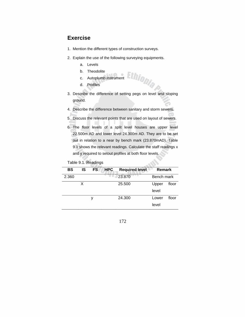
172
Exercise
1. Mention the different types of construction surveys.
2. Explain the use of the following surveying equipments.
a. Levels
b. Theodolite
c. Autoplumb instrument
d. Profiles
3. Describe the difference of setting pegs on level and sloping
ground.
4. Describe the difference between sanitary and storm sewers.
5. Discuss the relevant points that are used on layout of sewers.
6. The floor levels of a split level houses are upper level
22.500m AD and lower level 24.300m AD. They are to be set
out in relation to a near by bench mark (23.870mAD). Table
9.1 shows the relevant readings. Calculate the staff readings x
and y required to setout profiles at both floor levels.
Table 9.1. Readings
BS IS FS HPC Required level Remark
2.360 23.870 Bench mark
X 25.500 Upper floor
level
y 24.300 Lower floor
level
173
GLOSSARY
Accuracy: The conformity of the measurement to the true
value.
Alignment: the location of centerline of a survey or a facility.
Arithmetic Check: a check in the reductions of differential
leveling involving the sums of back sight and
foresights.
Automatic level: A surveyor’s level in which line of sight is
automatically maintained in the horizontal plane,
once the instrument is roughly leveled.
Azimuth: the angle to a line of sight, measures clockwise
(usually) from a north meridian.
Back sight: A sight taken with a level to a point of known
elevation, thus permitting the surveyor to compute
the elevation of the HI. In transit work, the back sight
is a sighting taken to a point of known position to
establish a reference direction.
Base line: A line of reference for survey work; often the
center line, the street line, or the center line of
construction is used, although any line could be
arbitrarily selected or established.
174
Batter Boards: Horizontal crosses pieces on grade stacks or
grade rods that refer to the proposed elevation.
Bearing: Direction of a line given by the acute angle from a
meridian and accompany by a cardinal compass
direction.
Bench mark: a relatively permanent object, natural or
artificial, is having a marked point whose elevation
above or below an adopted datum.
Construction Survey: Provision of line and grade.
Contour: A line on a map joining points of similar elevation.
Control Surveys: Surveys taken to establish reference
points, elevations and lines for preliminary and
construction surveys.
Cross section: a profile of the ground and surroundings
taken at right angles to a reference line.
Cut: In construction, the excavation of material; also the
measurement down from a grade mark.
Datum: An assumed or fixed horizontal reference plane.
Deflection angle: the angle between the prolongation of the
back line measured right (R) or left (L) to the forward
line.
175
Departure: The change in easterly displacement of a line
(ΔE).
Differential Leveling: Determining the differences in
elevation between points using surveyor’s level.
Double Centering: A technique of turning angles or
producing straight lines involving a minimum of two
sightings with a theodolite. Once with the telescope
direct and once with the telescope inverted.
Drainage: The collection and transportation of ground and
storm water.
Elevation: the vertical distance from a vertical datum, usually
sea level, to a point or object.
Fill: Material used to raise the construction level; also the
measurement up from a grade mark.
Foresight: In leveling, a sight taken from a BM or TP to
obtain a check on a leveling operation or to establish
a transfer elevation.
Free Station: A conveniently located instrument station used
for construction layout, the position of which is
determined after occupation through resection
techniques.
176
Gradient: The slope of a grade line.
Gunter’s Chain: Early (1800s) measuring devices consisting
of 100 links, measuring 66ft long.
Horizontal plane: a plane perpendicular to the direction of
gravity. In plane surveying, a plane perpendicular to
the plumb line.
Horizontal line: a line in a horizontal plane. In plane
surveying, a line is perpendicular to the vertical.
Intermediate Sight: A sight taken with a level or transit to
determine a feature elevation and or location.
Lay out Survey: Construction surevey.
Level surface: a curved surface that at every point is
perpendicular to the local plumb line (the direction of
gravity acts). They are approximately spheroid in
shape.
Level line: a line in a curved surface.
Leveling: the process of finding elevations of points, or their
difference in elevation.
Latitude (of a course): The change in northerly displacement
of a line (ΔN)
177
Latitude (geographic): angular distance from the earth’s
center, measured northerly or southerly from the
equatorial plane.
Line and Grade: The horizontal and vertical position of a
facility.
Linear Error of Closure: The line of traverse misclosure
representing the resultant of the measuring errors.
Longitude: angular distance measured in the plane of the
equator from the reference meridian through
Greenwich, England. Lines of longitude are indicated
on globes as meridians.
Mean sea level: The average height of the sea's surface for
all stages of tide over a 19-years period.
Meridian: A north-south reference line.
Mistake: a poor result due to carelessness or
misunderstanding.
Normal Tension: The amount of tension required in taping to
offsets the effects of Sag.
Original Ground: The position of the ground surface prior to
construction.
178
Page Check: Arithmetic Check.
Planimeter: A mechanical or electronic device used to
measure areas by tracing the out line of the area on
the map or plan.
Precision: The degree of refinement with which a
measurement is made.
Property Survey: A survey to retrace or establish property
lines, or to establish the location of buildings with in
the property limits.
Station: A point on a base line that is a specified distance
from the point of commencement. The point of
commencement is identified as 0+00; 100 ft or 100m
are known as full stations (1000m in some high way
applications); 1+45.20 identifies a point distant
145.20 ft or m from the point of commencement.
Traverse: a continuous series of measured (angle and
distance) lines.
Three-wire leveling: A more precise technique of differential
leveling in which rod readings are taken at the stadia
hairs, in addition to the main cross hair.
Total Station: An electronic theodolite combined with an
EDM and an electronic data collector.
179
Turning Point: In leveling a solid point where an elevation is
temporarily established so that the level may be
relocated.
Vertical Angle: An angle in the vertical plane measured up
(+) or down (-) from the horizontal.
Vertical control: a series of bench marks or other points of
known elevation established through out an area,
also called basic control or level control.
Vertical datum: any level surface to which elevations are
referred. Also called vertical datum plane.
Vertical line: a line that follows the direction of gravity as
indicated by a plumb line.
Vertical plane: At a point is any plane that contains the
vertical line at the point. There are unlimited number
of vertical planes at a given points.
Waving the rod: The slight waving of the leveling rod to and
from the instrument, which permits the surveyor to
take a precise (lowest) rod reading.
Zenith Angle: Vertical angle measured down ward from the
Zenith (Up wards plumb line) direction.
180
REFERENCES
1. Barry F. Kavanagh and S.J. Glenn Bird, Surveying
Principles and Applications, 5th edition, 2000.
2. Paul R. Wolf and Russell C. Brinker, Elementary
Surveying, 9th edition, 1994.
3. James M. Anderson and Edward M. Michael , Surveying
Theory and Practice, 7th Edition, 1998
4. William Irvine, Surveying for Construction, 4th Edition,
1995
5. Nathanson Kissam, Surveying Practice, 4th Edition, 1988
6. Francis H. Moffitt, Surveying, 8th ed. 1987.
7. R.Agor, A text book of Survying and Leveling, 9th ed.
2003.