learning to shadow hand-drawn sketches - arxiv · learning to shadow hand-drawn sketches qingyuan...

Learning to Shadow Hand-drawn Sketches

Qingyuan Zheng∗1, Zhuoru Li∗2, and Adam Bargteil1

1University of Maryland, Baltimore County2Project HAT

{qing3, adamb}@umbc.edu, [email protected]

Abstract

We present a fully automatic method to generate detailedand accurate artistic shadows from pairs of line drawingsketches and lighting directions. We also contribute a newdataset of one thousand examples of pairs of line draw-ings and shadows that are tagged with lighting directions.Remarkably, the generated shadows quickly communicatethe underlying 3D structure of the sketched scene. Con-sequently, the shadows generated by our approach can beused directly or as an excellent starting point for artists.We demonstrate that the deep learning network we proposetakes a hand-drawn sketch, builds a 3D model in latentspace, and renders the resulting shadows. The generatedshadows respect the hand-drawn lines and underlying 3Dspace and contain sophisticated and accurate details, suchas self-shadowing effects. Moreover, the generated shadowscontain artistic effects, such as rim lighting or halos ap-pearing from back lighting, that would be achievable withtraditional 3D rendering methods.

1. Introduction

Shadows are an essential element in both traditional anddigital painting. Across artistic media and formats, mostpaintings are first sketched with lines and shadows be-fore applying color. In both the Impressionism and Neo-classicism era, artists would paint oil paintings after theyrapidly drew shadowed sketches of their subjects. Theyrecorded what they saw and expressed their vision insketches and shadows and used these as direct referencesfor their paintings [1].

In the modern painting era, particularly for digital il-lustration and cel animation, shadows play an importantrole in depicting objects’ shapes and the relationships be-tween 2D lines and 3D space, thereby affecting the audi-

∗Equal contribution.

Figure 1: Top: our shadowing system takes in a line drawing anda lighting direction label, and outputs the shadow. Bottom: ourtraining set includes triplets of hand-drawn sketches, shadows, andlighting directions. Pairs of sketches and shadow images are takenfrom artists’ websites and manually tagged with lighting directionswith the help of professional artists. The cube shows how we de-note the 26 lighting directions (see Section 3.1). c©Toshi, ClementSauve

ence’s recognition of the scene as whole. Illustration is atime-consuming process; illustrators frequently spend sev-eral hours drawing an appealing picture, iteratively adjust-ing the form and structure of the characters many times.In addition to this work, the illustrators also need to itera-tively adjust and refine the shadows, either after completingthe sketch or while iterating the sketching process. Draw-ing shadows is particularly challenging for 2D sketches thatcannot be observed in the real world, because there is no3D reference model to reason about; only the artist’s imag-ination. In principal, the more details the structural linescontain, the more difficult it is to draw the resulting shad-ows. Hence adjusting the shadows can be time consuming,

arX

iv:2

002.

1181

2v2

[cs

.CV

] 2

Apr

202

0

especially for inexperienced illustrators.In this paper, we describe a real-time method to gener-

ate plausible shadows from an input sketch and specifiedlighting direction. These shadows can be used directly, orif higher quality is desired can be used as a starting pointfor the artists to modify. Notably, our approach does notgenerate shadowed sketches directly; instead it generates aseparate image of the shadow that may be composited withthe sketch. This feature is important as the artist can loadthe sketch and the shadow into separate image layers andedit them independently.

Our work uses the deep learning methodology to learna non-linear function which “understands” the 3D spatialrelationships implied by a 2D sketch and render the binaryshadows (Figure 1 top). The raw output from our neural net-work is binary shadows, which may be modified by artistsin a separate layer independent of line drawings. There is noadditional post-processing and the images in our paper aresimple composites of the raw network outputs and the inputline drawings. If soft shadows are desired, artists may usethe second intermediate output from our network (Figure 2s2). Our network also produces consistent shadows fromcontinuously varying lighting directions (Section 4.3), eventhough we train from a discrete set of lighting directions.

Given a line drawing and a lighting direction, our modelautomatically generates an image where the line drawing isenhanced with detailed and accurate hard shadows; no ad-ditional user input is required. We focus on 2D animationstyle images (e.g. Japanese comic, Inker [37]) and the train-ing data is composed of artistic hand-drawn line drawing inthe shape of animation characters, mecha, and mechanicalobjects. We also demonstrate that our model generalizes toline drawing of different objects such as buildings, clothes,and animals.

The term “artistic shadow” in our work refers to binaryshadows that largely obey physics but also have artistic fea-tures such as less shadowing of characters’ faces and rimlighting when characters are back lit.

The main contributions of our work:

• We created a new dataset that contains 1,160 cases ofhand-drawn line drawings and shadows tagged withlighting directions.

• We propose a network that “understands” the structureand 3D spatial relationships implied by line drawingsand produces highly-detailed and accurate shadows.

• An end-to-end application that can generate binary orsoft shadows from arbitrary lighting directions given a2D line drawing and designated lighting direction.

In Section 3, we will decribe the design of our genera-tive and discriminator networks, and our loss functions. In

Section 4, we compare our results quantitatively and qual-itatively to baseline network architectures pix2pix [16] andU-net [28]. We also compare to the related approachesSketch2Normal [32] and DeepNormal [14] applied to ourshadow generation problem. Our comparisons include asmall user study to assess the perceptual accuracy of ourapproach. Finally, we demonstrate the necessity of eachpart of our proposed network through an ablation study andmetrics analysis. 1

2. Related Work

Non-photorealistic rendering in Computer Graph-ics. The previous work on stylized shadows [26, 3] for celanimation highlights that shadows play an important role inhuman perception of cel animation. In particular, shadowsprovide a sense of depth to the various layers of character,foreground, and background. Lumo [17] approximates sur-face normals directly from line drawings for cel animationto incorprate subtle environmental illumination. Todo et al.[35, 36] proposed a method to generate artistic shadows in3D scenes that mimics the aesthetics of Japanese 2D anima-tion. Ink-and-Ray [34] combined a hand-drawn characterwith a small set of simple annotations to generate bas-reliefsculptures of stylized shadows. Recently, Hudon et al. [13]proposed a semi-automatic method of cel shading that pro-duces binary shadows based on hand-drawn objects without3D reconstruction.

Image translation and colorization. In recent years,the research on Generative Adversarial Networks (GANs)[7, 24] in image translation [16] has generated impressivesynthetic images that were perceived to be the same as theoriginals. Pix2pix [16] deployed the U-net [28] architec-ture in their Generator network and demonstrated that forthe application of image translation U-net’s performance isimproved when skip connections are included. CycleGAN[44] introduced a method to learn the mapping from an in-put image to a stylized output image in the absence of pairedexamples. Reearch on colorizing realistic gray scale images[2, 42, 15, 43] demonstrated the feasibility of colorizing im-ages using GANs and U-net [28] architectures.

Deep learning in line drawings. Researcher that con-siders line drawings include line drawing colorization [39,19, 41, 5, 4], sketch simplification [31, 29], smart inker [30],line extraction [21], line stylization [22] and computing nor-mal maps from sketches [32, 14]. Tag2Pix [19] seeks touse GANs that concatenate Squeeze and Excitation [12] tocolorize line drawing. Sketch simplification [31, 29] cleansup draft sketches, through such operations as removing duallines and connecting intermittent lines. Smart inker [30] im-proves on sketch simplification by including additional user

1Project page is at https://cal.cs.umbc.edu/Papers/Zheng-2020-Shade/.

https://cal.cs.umbc.edu/Papers/Zheng-2020-Shade/

https://cal.cs.umbc.edu/Papers/Zheng-2020-Shade/

input. Users can draw strokes indicating where they wouldlike to add or erase lines, then the neural network will out-put a simplified sketch in real-time. Line extraction [21]extracts pure lines from manga (comics) and demonstratesthat simple downscaling and upscaling residual blocks withskip connections have superior performance. Kalogerakiset al. [18] proposed a machine learning method to createhatch-shading style illustrations. Li et al. [22] proposed atwo-branch deep learning model to transform the line draw-ings and photo to pencil drawings.

Relighting. Deep learning has also been applied to re-lighting realistic scenes. Xu et al. [38] proposed a methodfor relighting from an arbitrary directional light given im-ages from five different directional light sources. Sun et al.[33] proposed a method for relighting portraits given a sin-gle input, such as a selfie. The training datasets are capturedby a multi-camera rig. This work differs from ours in thatthey focus on relighting realistic images while we focus onartistic shadowing of hand-drawn sketches.

Line drawings to normal maps. Sketch2normal [32]and DeepNormal [14] use deep learning to compute nor-mal maps from line drawings. Their training datasetsare rendered from 3D models with realistic rendering.Sketch2Normal trains on line drawings of four-legged an-imals with some annotations. DeepNormal takes as inputline drawings with a mask for the object. They solve a dif-ferent, arguably harder, problem. However, the computednormal maps can be used to render shadows and we com-pare this approach to our direct shadow computation in Sec-tion 4. Given color input images, Gao and colleagues [6]predict normal maps and then generate shadows.

3. Learning Where to Draw ShadowsIn this section we describe our data preparation, our rep-

resentation of the lighting directions, the design of our gen-erator and discriminator networks, and our loss functions.

3.1. Data Preparation

We collect our (sketch, shadow) pairs from website postsby artists. With help from professional artists, each (sketch,shadow) pair is manually tagged with a lighting direction.After pre-processing the sketches with thresholding andmorphological anti-aliasing, the line drawings are normal-ized to obtain a consistent line width of 0.3 px in cairosvgstandard [27]. To standardize the hand-drawn sketch to thesame line width, we use a small deep learning model similarto smart inker [30] to pre-process input data. Our datasetcontains 1,160 cases of hand-drawn line drawings. Eachline drawing matches one specific hand-drawn shadow asground truth and one lighting direction.

In contrast to 3D computer animation, which containsmany light sources and realistic light transport, 2D anima-tion tends to have a single lighting direction and include

some non-physical shadows in a scene.We observed that artists tend to choose from a relatively

small set of specific lighting directions, especially in comicsand 2D animation. For this reason, we define 26 lighting di-rections formed by the 2×2 cube in Figure 1. We found thatit was intuitive to allow users to choose from eight lightingdirections clockwise around the 2D object and one of threedepths (in-front, in-plane, and behind) to specify the lightsource. We also allow the user to choose two special loca-tions: directly in front and directly behind. This results in8 × 3 + 2 = 26 lighting directions. The user specifies thelight position with a three-digit string. The first digit cor-responds to the lighting direction (1-8), the second to theplane (1-3), and the third is ’0’ except for the special direc-tions, which are “001” (in-front) and “002” (behind).

While users found this numbering scheme intuitive, weobtained better training results by first converting thesestrings to 26 integer triples on the cube from [−1, 1]3((0, 0, 0) is not valid as that is the location of the object).For example, “610” is mapped to (−1,−1,−1), “230” ismapped to (1, 1, 1), and “210” is mapped to (1, 1,−1).

3.2. Network Architecture

Our generator incorporates the following modules:residual blocks [9] [10], FiLM [25] residual blocks, andSqueeze-and-Excitation (SE) blocks [12]. The general ar-chitecture of our generator follows the architecture of U-net with skip connections [28, 16]. Our Discriminator usesresidual blocks. Details are shown in Figure 2.

3.2.1 Generative Network

We propose a novel non-linear model with two parts -ShapeNet, which encodes the underlying 3D structure from2D sketches, and RenderNet, which renders artistic shadowsbased on the encoded structure.

ShapeNet encodes a line drawing of an object into a highdimensional latent space and represents the object’s 3D ge-ometric information. We concatenate 2D coordinate chan-nels [23] to the line drawings to assist ShapeNet in encoding3D spatial information.

RenderNet performs reasoning about 3D shadows. Start-ing from the bottle neck, we input the embedded lighting di-rection using the normalization method from FiLM residualblocks [25]. The model then starts to learn the relationshipbetween the lighting direction and the various high dimen-sional features. We repeatedly add the lighting directioninto each stage of the RenderNet to enhance the reasoning ofdecoding. In the bottom of each stage in RenderNet, a Self-attention [40] layer complements the connection of holisticfeatures.

The shadowing problem involves holistic visual reason-ing because shadows can be cast by distant geometry. For

512 512 512 256 128 64 32 1664 128 256 51232 64 128 256 51232

Light Pos FC 128

Stan

dariz

ation

DecoderFeature

EncoderFeature SE Block

Concat FiLM ResiBlock

Light Pos

ResiBlock ResiBlock Self Atten DecoderFeature

EncoderFeature

Global Pool FC FC

Conv 1×1 Sigmoid

Sigmoid ×

×+

SE Block

Downscale ResiBlock ResiBlockResiBlock

Global PoolFC 256FC 1

Downscale ResiBlock ResiBlock

Self Attention Layer2D Coordinate

s1

s2

ShapeNet RenderNet Discriminator

s1

s2

Com

posit

ion

UpscaleResiBlock

Tiled Light Pos

Figure 2: Our GANs architecture. The line drawings are standardized first (same as in Section 3.1) before being inputted into the ShapeNet.Lighting directions are repeatedly added into the FiLM residual block in each stage in RenderNet. s1 and s2 are the up-sampled intermediateoutputs from the second and the forth stage in RenderNet. In the training process, the line drawings and pure shadows are inverted fromblack-on-white to white-on-black. More details are in supplementary material.

this reason we deploy Self-attention layers [40] and FiLMresidual blocks [25] to enhance the visual reasoning; net-works that consist of only residual blocks have limited re-ceptive fields and are ill-suited to holistic visual reasoning.The SE [12] blocks filter out unnecessary features importedfrom the skipped encoder output.

We also extract two supervision intermediate outputs, s1and s2, to facilitate backpropagation. Early stages of ourRenderNet generate continuous, soft shadow images. In thefinal stage, the network transforms these images to binaryshadows. The quality of the soft shadows in the interme-diate outputs, s1 and s2, is shown in Figure 2. We noteagain that our output does not require any post processingto generate binary shadows; the images in this paper resultdirectly from compositing the output our generator with theinput sketch.

3.2.2 Discriminator Network

The basic modules of our discriminator include down-scaling residual blocks and residual blocks. Since many lo-cal features of different shadows are similar to one another,we deploy Self-attention layers to make our discriminatorsensitive to the distant features. In Figure 2, the last of thediscriminator consists of global average pooling, dropoutwith 0.3 probabilities, and a fully connected layer with 256filters. Because generating shadows is more difficult thandiscriminating between fake and real shadows, a simple dis-criminator is sufficient and simplifies training.

3.3. Loss Function

The adversarial loss of our Generative Adversarial Net-work can be expressed as

LcGAN (G,D) = Ex,y,z [logD (C (x, y) , z)]

+Ex,z [log (1−D (C (x,G (x, z)) , z))] ,(1)

where x is the sketch, y is the ground truth shadow, and z isthe lighting direction. C(·) is a function that composite theground truth shadow and the input sketch as a “real” image,and composite the generated shadow and the input sketch asa “fake” image.

The generatorG aims to minimize the loss value, and thediscriminator D aims to maximize the loss value. For theloss value of our generator network, we add MSE losses ofthe two deep supervised outputs, which are the intermediateoutputs of the first and third stage in the decoder, to the lossof the generator’s final output.

The three losses of the generator network can be ex-pressed as

Loutput(G) = Ex,y,z

[‖y −G(x, z)‖22

]+ ξ · TV (G(x, z)) ,

(2)where Loutput is the loss between generated shadow andthe ground truth. Loutput consists of a total variation (TV)regularizer and an MSE loss. The TV regularizer, weightedby ξ, encourages smooth details around the boundaries ofshadows. We set ξ to 2 × 10−6, a 5× smaller value thanthe total number of pixels in the input sketch. We will showhow the value of ξ affects the final output in the ablationstudy. The deep supervised outputs are upsampled and theirlosses are computed as by MSE loss from ground truth,

Lsi (G) = Ex,y,z

[‖y −Gsi(x, z)‖

22

], i = 1, 2. (3)

Final objective is the sum of Loutput, Ls1 , Ls2 , and theLcGAN ,

G∗ = argminG

maxD

λ1LcGAN (G,D)

+λ2Loutput (G) + λ3Ls1 (G) + λ4Ls2 (G) .(4)

In our experiments, the four losses are weighted by λ1 =0.4, λ2 = 0.5, λ3 = 0.2, and λ4 = 0.2.

Input Ours DeepNormal Sketch2Normal DeepNormal Sketch2NormalOursInput610

210

810

710 710

210

310

710

Figure 3: Shadows for lighting depth “1” - in front of the plane (front lighting), compared with previous work DeepNormal [14] andSketch2Normal [32]. The little sun denotes the lighting direction. c©Derori-san, Imomushi-san, Eric ou

4. Experiments and EvaluationIn this section, we evaluate the performance of our shad-

owing model. In particular, we discuss implementation de-tails, provide comparisons with the baseline pix2pix [16]and U-net [28] and the previous work DeepNormal [14] andSketch2Normal [32], describe a small user study, and detailour ablation study.

4.1. Implementation Details

All the lines of sketch images in our dataset are normal-ized and thinned to produce a standard data representation.If the user input sketch is not normalized and thinned, weapply a pre-trained line normalization model modified from[30] to preprocess the user input.

In the training process, the line drawings are first in-verted from black-on-white to white-on-black and input tothe network. The final output and the intermediate outputss1 and s2 from the generator are similarly white shadowson black backgrounds. Inverting the images causes the net-work to converge faster. The generated shadows are com-posited with the line drawings as the “fake” image input tothe discriminator. Similarly we composite the sketch andpure shadow in our dataset as the “real” image input to dis-criminator.

Because of limited size of our dataset of sketch/shadowpairs with annotated lighting direction we used the entire

dataset for training—we did not reserve any of our trainingdataset for testing. We trained for 80, 000 iterations withAdam optimizer [20]. The optimizer parameters are set tolearning rate = 0.0002, β1 = 0, and β2 = 0.9. The net-work is trained using one 12G Titan Xp with a batch size of8 and 320× 320 input image size.

We shift, zoom in/out, and rotate to augment our dataset.When we rotate our line drawing input by each of {0, 45, 90,135, 180, 225, 270, 315} degrees, we also rotate the groundtruth shadow images and modify the lighting direction la-bels, by adding 1 to the first digit for every 45 degrees ofrotation. Shifting and zooming does not affect the lightingdirection.

4.2. Comparison with Prior Work

In this subsection, we qualitatively compare our ap-proach to DeepNormal [14] and Sketch2Normal [32]. Also,we compare our network to two baselines, Pix2pix [16] andU-net [28]. The evaluation dataset is not included in train-ing. The line drawings (without shadows) used for evalua-tion are collected from other artists and prior work to whichwe compare.

We generated the output from DeepNormal andSketch2Normal using their source codes and trained mod-els, unmodified. We use the scripts provided by Deep-Normal to render shadows from normal maps. All nor-

Input Ours DeepNormal Sketch2Normal

220

620

Figure 4: Comparisons with previous works DeepNormal [14] andSketch2Normal [32] with lighting depth “2” - in the plane (sidelighting). The little sun denotes the lighting direction.

Input Ours DeepNormal Sketch2Normal630

Figure 5: Comparison with DeepNormal [14] and Sketch2Normal[32] when the light’s depth is “3” - behind the plane (back light-ing). Our approach demonstrates rim lighting.

mal maps are rendered under the same settings in this pa-per. To generate binary shadows, we threshold the contin-uous shadings at 0.5. We note that DeepNormal addition-ally requires a mask to eliminate space outside the object;Sketch2Normal and our work do not require this mask. Weprovide a hand-drawn mask as input to DeepNormal. Ourmethod and DeepNormal are predicted from 320 × 320 in-puts and Sketch2Normal is predicted from 256 × 256 in-puts. Since DeepNormal claims their results are consistentin various size of input, and Sketch2Normal experiment in256× 256 inputs.

As shown in Figure 3, 4, 6, 5, 7, our work performsfavorably. For example, on the two-people and multiple-people line drawings (Figure 3 second row), our work isable to shadow each character, however, DeepNormal andSketch2Normal treat multiple people as one object. No-tably, our work is superior in generating highly detailedshadows, such as in girl’s hair and skirt. In terms of thecomplexity of sketch, though our training datasets have amoderate level of detail, our network performs well on com-plex sketches as shown in Figure 3. We also perform wellbeyond the object’s boundary without requiring a mask.

Moreover, our work produces more precise details whenthe light source changes depth. As we can see in Figure 4,the shadows from DeepNormal [14] cover almost the en-tire image, so that it seems as though the light is behind

Sketch [14]-normal [32]-normal 3D model GT-normal

Ours-120 [14]-120 [32]-120 GT3D-120 GT-120

Ours-220 [14]-220 [32]-220 GT3D-220 GT-220

Figure 6: Comparisons between ground truth (GT), our approach,DeepNormal [14], and Sketch2Normal [32] rendered with a 3Dbunny, with lighting depth “2”. “120”: top, side lighting. “220”:upper right, side lighting. “GT3D”: rendered from commercial 3Dsoftware. “GT”: rendered from its normal map.

the object. However, in these images, the light source is inthe same plane as the object, resulting in side lighting. InFigure 6, we explain why DeepNormal [14] underperformswhen the light is in the object’s plane by comparing with a3D test model. In particular, using our technique the shad-ows on the bunny’s head and leg are closer to the groundtruth and demonstrate self-shadowing. As highlighted inFigure 4, DeepNormal’s normal maps have low variancedue to multiple average of 256 × 256 tiles (refer to sec-tion 3.4 of DeepNormal). This low variance results in frontlighting appearing to be side lighting and side lighting ap-pearing to be back lighting. Some images generated bySketch2Normal have some artifacts because the predictednormal maps have some blank areas. Because it is trainedon simple sketches, Sketch2Normal struggles with complexsketches. Finally, we note that our approach produces artis-tic rim highlights from back lighting. Please refer to thesupplementary material for the normal maps in Figure 3 andmore comparison figures.

Our architecture also performs favorable when qualita-tively compared to Pix2pix and U-net trained on our dataset(Figure 7). Generally, U-net generates inaccurate soft shad-ows that are far from our goal of binary shadows. Pix2pixgenerates shadows far outside the object’s boundary andignores the geometric information in the sketch. In ourearly research, we used a residual block autoencoder withskip connections, which generated soft shadows. To achieveour goal of binary shadows, we added a discriminator andadopted a deeper RenderNet. If the artist desires soft shad-ows, the intermediate output s2 can be used.

Input Ours Pix2pix U-net210

Figure 7: Comparison with Pix2pix [16] and U-net [28] architec-tures trained on our dataset. Light depth is “1”.

(b) (c) (d)

(e) (f) (g) (h)

(a)

Figure 8: Combining our shadows with color. (a) Input sketch.(b) Our shadow with lighting direction “710”. (c) Our shadowsin complex lighting conditions created by compositing shadowsfrom “001”, “730”, and “210”. (d) Our shadows composited fromlighting directions “001”, “210”, “220” with dots and soft shadowto produce a manga style. (e) Colorized sketch with commercialsoftware. (f) Composite of (e) and (b). (g) Composite of (e) and(c). (h) Original artist’s image. c©nico-opendata

4.3. Artistic Control

Though our network is trained with a discrete set of 26lighting directions, the lighting direction is inputted to thenetwork using floating point values in [−1, 1]3, allowing forthe generation of shadows from arbitrary light locations. In-tuitively, our network learns a continuous representation oflighting direction from the discrete set of examples. Fur-thermore, when a series of light locations are chosen theshadows move smoothly over the scene as in time-lapsevideo footage. Please refer to the supplementary materialfor gifs demonstrating moving shadows.

Although the final output of our network is binary shad-ows, if an artist desires soft shadows, the intermediate out-put, s2, can be used, as shown in Figure 2.

Our work is complementary to prior work on automaticcolorization of sketches [39, 19, 41, 5, 4]. Figure 8 demon-strates that our shadows can be combined with these col-orization approaches. While most prior work on coloriza-tion combines shading and shadowing effects, it would beinteresting to separate these effects into indpendent imagelayers for further artistic editing.

Methods GT Ours [14] [32] [16] [28]

Turing 68% 69% 51% 11% 23% 19%Scores 6.37 6.70 5.78 3.35 3.77 3.06

Methods GT Ours [14] [32] [16] [28]

Turing 70% 65% 45% 10% 25% 17%Scores 6.50 6.66 5.69 3.44 3.91 3.03

Table 1: Results of user study comparing Ground truth (GT) in ourdatasets, Ours, DeepNormal [14], Sketch2Normal [32], Pix2pix[16] baseline and U-net [28] baseline. First row: percentage thatpass the Turing test. Second row: average scores. 9 is the bestscore. Top: total results. Bottom: results of people with drawingexperience.

4.4. User Study

To evaluate our approach we conducted a small userstudy. We generated shadows using six different techniquesand asked users to evaluate the results. We train the userswith some samples from our dataset at the beginning. Ouruser study had two stages: a “Turing” test that asked thesimple question “Do you think this shadow was drawn bya human? Yes or no?” and another stage where the user isshown an image and asked to rate the quality of the shadowwith the prompt “Under this lighting direction, evaluatethe appearance of this shadow” on a Likert scale from 1to 9 (9 being best). In each stage the user was shown 36images generated from six input sketches and each of sixshadow generation methods: ground truth shadows createdby artists, Ours, DeepNormal [14], Sketch2Normal [32],Pix2pix [16], and U-net [28]. For the synthetic shadows,the lighting directions were chosen randomly (Ours excludethe directions in ground truth), with the restriction that wedid not use back lighting. We only used front lighting forDeepNormal for the reasons described in Section 4.2. Forthe quality rating, lighting directions were described withtext, e.g. “upper right, front lighting.” For the Turing test,no lighting directions were given. Users were shown oneimage at a time, but could use the “back” and “forward”buttons.

Users received a brief training that displayed 15 groundtruth shadowed sketches from our dataset and highlightedthe differences between front lighting and side lighting. Wealso asked the users to rate their drawing experience as “pro-fessional”, “average”, “beginner” or “0 experience”. Wedistributed the survey online and received 60 results. Fortyparticipants had drawing experience: 13 were professionalartists, 11 were average level, and 16 were beginners. Theresults are shown in Table 1. Our approach performs fa-vorably, almost matching the ground truth shadows createdby artists. We ran a one-way ANOVA to analyze the Likert

Figure 9: FID scores of ours and ablation studies. Our model’sline is on the most bottom.

(a) ours (b) w/o SA (c) w/o CC (d) w/o FiLM

(e) w/o SE (f) w/o s1, s2 (g) TV = 5× (h) w/o TV

Figure 10: Ablation studies. (b) removing the Self-attention (SA)layers, (c) removing the Coordinate Channel (CC), (d) removingthe FiLM residual blocks, (e) removing the SE blocks, (f) remov-ing the two deep supervised outputs (s1, s2), (g) increasing the TVloss weights to e−5, (h) removing the total variant (TV) regular-izer.

scores. The results confirmed that our results were quantita-tively similar to ground truth (p = 0.24) and better than theother methods (p < 0.05 for all of the comparisons). Pleaserefer to the supplementary material for more details of thestatistical significance report of our user study.

4.5. Ablation Study

We performed seven ablation studies as shown in Fig-ures 10 and 9. For quantitative comparison, we calculatedthe Frechet Inception Distance (FID) [11] per 4000 itera-tions of our work and the ablation studies using the entiredataset. Figure 9 shows that our work has the lowest andmost stable FID. This demonstrate that each feature we pro-pose is essential and that the total variation regularizer wascritically important.

Figure 10 qualitatively demonstrates that without the el-ements we propose, the networks performance is degraded:

boundaries become aliased and artifacts appear in shadows.Among all ablation studies, “w/o Self-attention” has theleast influence, as the shown Figure 10 (b) and the FID inFigure 9. Setting the coefficient of the total variation regu-larizer 5× larger or removing the regularizer has the mostinfluence on the overall performance and ruins the smooth-ness of shadow. The corresponding FID also highlight theimportance of the total variant regularizer.

In Figure 10, all of the images use the same lightingdirection “810”. Generally, when the Self-attention lay-ers are removed, the network performs poorly with detailsand there are tiny artifacts within the shadow block; withoutthe Coordinate Channel or FiLM residual block, the outputwill have unrealistic shadow boundaries and shadows out-side the object’s boundary; without SE blocks, there willbe shadow “acne” and the overall appearance looks messy;without the two deep supervised outputs (λ1 = .4, λ2 = .9,λ3 = λ4 = 0), the output will have dot artifacts in a gridpattern and lower accuracy; if the network has 5× higherweight for the TV regularizer or is missing the TV regular-izer, the network will converge too fast and trap in a localminimum.

5. Future Work

The network performance is not invariant on differentsizes of input images. Mostly the 320 × 320 inputs havethe best performance, because our network is trained on320 × 320 size inputs. 480 × 480 input images also havegood performance. Though we almost match the groundtruth in user study, our generated shadows are not so muchdetailed as ground truth, especially on hard surface object(e.g. desk, laptop). Also, if inputting a local part of the linedrawing, the network is not able to reason the correct shad-ows. As future work, we will develop a network that canoutput various image sizes to meet the high resolution re-quirements of painting.

6. Conclusion

Our conditional Generative Adversarial Network learnsa non-photorealistic renderer that can automatically gener-ate shadows from hand-drawn sketches. We are the first toattempt to directly generate shadows from sketches throughdeep learning. Our results compare favorably to prior artthat renders normal maps from sketches on both simple andsophisticated images. We also demonstrate that our networkarchitecture can “understand” the 3D spatial relationshipsimplied by 2D line drawings well enough to generate de-tailed and accurate shadows.

Acknowledgements: The authors wish to thank YuchenMa and Kejun Liu for annotating the dataset and the review-ers, Tiantian Xie, and Lvmin Zhang for many suggestions.

References[1] Rudolf Arnheim. Art and visual perception: A psychology of

the creative eye. Univ of California Press, 1965.[2] Zezhou Cheng, Qingxiong Yang, and Bin Sheng. Deep col-

orization. In Proceedings of the IEEE International Confer-ence on Computer Vision, pages 415–423, 2015.

[3] Christopher DeCoro, Forrester Cole, Adam Finkelstein, andSzymon Rusinkiewicz. Stylized shadows. In Proceedings ofthe 5th international symposium on Non-photorealistic ani-mation and rendering, pages 77–83. ACM, 2007.

[4] Kevin Frans. Outline colorization through tandem adversar-ial networks. arXiv preprint arXiv:1704.08834, 2017.

[5] Chie Furusawa, Kazuyuki Hiroshiba, Keisuke Ogaki, andYuri Odagiri. Comicolorization: semi-automatic mangacolorization. In SIGGRAPH Asia 2017 Technical Briefs,page 12. ACM, 2017.

[6] Zhengyan Gao, Taizan Yonetsuji, Tatsuya Takamura, ToruMatsuoka, and Jason Naradowsky. Automatic illuminationeffects for 2d characters. In NIPS Workshop on MachineLearning for Creativity and Design, 2018.

[7] Ian Goodfellow, Jean Pouget-Abadie, Mehdi Mirza, BingXu, David Warde-Farley, Sherjil Ozair, Aaron Courville, andYoshua Bengio. Generative adversarial nets. In Advancesin neural information processing systems, pages 2672–2680,2014.

[8] Todd Goodwin, Ian Vollick, and Aaron Hertzmann. Isophotedistance: a shading approach to artistic stroke thickness.In Proceedings of the 5th international symposium on Non-photorealistic animation and rendering, pages 53–62. ACM,2007.

[9] Kaiming He, Xiangyu Zhang, Shaoqing Ren, and Jian Sun.Deep residual learning for image recognition. In The IEEEConference on Computer Vision and Pattern Recognition(CVPR), June 2016.

[10] Kaiming He, Xiangyu Zhang, Shaoqing Ren, and Jian Sun.Identity mappings in deep residual networks. In ECCV,2016.

[11] Martin Heusel, Hubert Ramsauer, Thomas Unterthiner,Bernhard Nessler, and Sepp Hochreiter. Gans trained by atwo time-scale update rule converge to a local nash equilib-rium. In Advances in Neural Information Processing Sys-tems, pages 6626–6637, 2017.

[12] Jie Hu, Li Shen, and Gang Sun. Squeeze-and-excitation net-works. In IEEE Conference on Computer Vision and PatternRecognition, 2018.

[13] Matis Hudon, Rafael Pages, Mairead Grogan, Jan Ondrej,and Aljosa Smolic. 2d shading for cel animation. In Pro-ceedings of the Joint Symposium on Computational Aesthet-ics and Sketch-Based Interfaces and Modeling and Non-Photorealistic Animation and Rendering, page 15. ACM,2018.

[14] Matis Hudon, Rafael Pages, Mairead Grogan, and AljosaSmolic. Deep normal estimation for automatic shading ofhand-drawn characters. In ECCV Workshops, 2018.

[15] Satoshi Iizuka, Edgar Simo-Serra, and Hiroshi Ishikawa. Letthere be Color!: Joint End-to-end Learning of Global and

Local Image Priors for Automatic Image Colorization withSimultaneous Classification. ACM Transactions on Graphics(Proc. of SIGGRAPH 2016), 35(4):110:1–110:11, 2016.

[16] Phillip Isola, Jun-Yan Zhu, Tinghui Zhou, and Alexei AEfros. Image-to-image translation with conditional adversar-ial networks. In 2017 IEEE Conference on Computer Visionand Pattern Recognition (CVPR), pages 5967–5976. IEEE,2017.

[17] Scott F Johnston. Lumo: illumination for cel animation.In Proceedings of the 2nd international symposium on Non-photorealistic animation and rendering, pages 45–ff, 2002.

[18] Evangelos Kalogerakis, Derek Nowrouzezahrai, SimonBreslav, and Aaron Hertzmann. Learning hatching forpen-and-ink illustration of surfaces. ACM Transactions onGraphics (TOG), 31(1):1, 2012.

[19] Hyunsu Kim, Ho Young Jhoo, Eunhyeok Park, and SungjooYoo. Tag2pix: Line art colorization using text tag with secatand changing loss. In Proceedings of the IEEE InternationalConference on Computer Vision, pages 9056–9065, 2019.

[20] Diederik P Kingma and Jimmy Ba. Adam: A method forstochastic optimization. arXiv preprint arXiv:1412.6980,2014.

[21] Chengze Li, Xueting Liu, and Tien-Tsin Wong. Deep extrac-tion of manga structural lines. ACM Transactions on Graph-ics (TOG), 36(4):117, 2017.

[22] Yijun Li, Chen Fang, Aaron Hertzmann, Eli Shechtman, andMing-Hsuan Yang. Im2pencil: Controllable pencil illustra-tion from photographs. In Proceedings of the IEEE Con-ference on Computer Vision and Pattern Recognition, pages1525–1534, 2019.

[23] Rosanne Liu, Joel Lehman, Piero Molino, Felipe PetroskiSuch, Eric Frank, Alex Sergeev, and Jason Yosinski. Anintriguing failing of convolutional neural networks and thecoordconv solution. In Advances in Neural Information Pro-cessing Systems, pages 9628–9639, 2018.

[24] Mehdi Mirza and Simon Osindero. Conditional generativeadversarial nets. arXiv preprint arXiv:1411.1784, 2014.

[25] Ethan Perez, Florian Strub, Harm De Vries, Vincent Du-moulin, and Aaron Courville. Film: Visual reasoning with ageneral conditioning layer. In Thirty-Second AAAI Confer-ence on Artificial Intelligence, 2018.

[26] Lena Petrovic, Brian Fujito, Lance Williams, and AdamFinkelstein. Shadows for cel animation. In Proceedings ofthe 27th annual conference on Computer graphics and in-teractive techniques, pages 511–516. ACM Press/Addison-Wesley Publishing Co., 2000.

[27] Python. Cairosvg, 2019. https://cairosvg.org/.[28] Olaf Ronneberger, Philipp Fischer, and Thomas Brox. U-

net: Convolutional networks for biomedical image segmen-tation. In International Conference on Medical image com-puting and computer-assisted intervention, pages 234–241.Springer, 2015.

[29] Edgar Simo-Serra, Satoshi Iizuka, and Hiroshi Ishikawa.Mastering sketching: adversarial augmentation for struc-tured prediction. ACM Transactions on Graphics (TOG),37(1):11, 2018.

https://cairosvg.org/

[30] Edgar Simo-Serra, Satoshi Iizuka, and Hiroshi Ishikawa.Real-time data-driven interactive rough sketch inking. ACMTransactions on Graphics (TOG), 37(4):98, 2018.

[31] Edgar Simo-Serra, Satoshi Iizuka, Kazuma Sasaki, and Hi-roshi Ishikawa. Learning to simplify: fully convolutionalnetworks for rough sketch cleanup. ACM Transactions onGraphics (TOG), 35(4):121, 2016.

[32] Wanchao Su, Dong Du, Xin Yang, Shizhe Zhou, and HongboFu. Interactive sketch-based normal map generation withdeep neural networks. Proceedings of the ACM on ComputerGraphics and Interactive Techniques, 1(1):22, 2018.

[33] Tiancheng Sun, Jonathan T Barron, Yun-Ta Tsai, ZexiangXu, Xueming Yu, Graham Fyffe, Christoph Rhemann, JayBusch, Paul Debevec, and Ravi Ramamoorthi. Single imageportrait relighting. ACM Transactions on Graphics (TOG),38(4):79, 2019.

[34] Daniel Sykora, Ladislav Kavan, Martin Cadık, OndrejJamriska, Alec Jacobson, Brian Whited, Maryann Simmons,and Olga Sorkine-Hornung. Ink-and-ray: Bas-relief meshesfor adding global illumination effects to hand-drawn charac-ters. ACM Transactions on Graphics (TOG), 33(2):16, 2014.

[35] Hideki Todo, Ken Anjyo, and Shunichi Yokoyama. Lit-sphere extension for artistic rendering. The Visual Computer,29(6-8):473–480, 2013.

[36] Hideki Todo, Ken-ichi Anjyo, William Baxter, and TakeoIgarashi. Locally controllable stylized shading. ACM Trans.Graph., 26(3):17, 2007.

[37] Wikipedia. Inker, 2019. https://en.wikipedia.org/wiki/Inker.

[38] Zexiang Xu, Kalyan Sunkavalli, Sunil Hadap, and RaviRamamoorthi. Deep image-based relighting from optimalsparse samples. ACM Transactions on Graphics (TOG),37(4):126, 2018.

[39] Taizan Yonetsuji. Paintschainer, 2017.https://paintschainer.preferred.tech/.

[40] Han Zhang, Ian Goodfellow, Dimitris Metaxas, and Augus-tus Odena. Self-attention generative adversarial networks.arXiv preprint arXiv:1805.08318, 2018.

[41] Lvmin Zhang, Chengze Li, Tien-Tsin Wong, Yi Ji, andChunping Liu. Two-stage sketch colorization. In SIG-GRAPH Asia 2018 Technical Papers, page 261. ACM, 2018.

[42] Richard Zhang, Phillip Isola, and Alexei A Efros. Colorfulimage colorization. In European Conference on ComputerVision, pages 649–666. Springer, 2016.

[43] Richard Zhang, Jun-Yan Zhu, Phillip Isola, Xinyang Geng,Angela S Lin, Tianhe Yu, and Alexei A Efros. Real-timeuser-guided image colorization with learned deep priors.ACM Transactions on Graphics (TOG), 9(4), 2017.

[44] Jun-Yan Zhu, Taesung Park, Phillip Isola, and Alexei AEfros. Unpaired image-to-image translation using cycle-consistent adversarial networks. In Proceedings of the IEEEinternational conference on computer vision, pages 2223–2232, 2017.

https://en.wikipedia.org/wiki/Inker

https://en.wikipedia.org/wiki/Inker

Appendix

A. Lighting DirectionsWe found ‘810’ numbering scheme to be more intuitive

for the users than the other two methods ([−1, 0, 1]3 or aninteger between 1 and 26). Therefore, we use ‘810’ schemeas the user inputs, then transfer the ‘810’ scheme (first col-umn of Table 2) to the [−1, 0, 1]3 scheme (third column ofTable 2) in programming.

Label Direction Position

001 rear center [0,0,1]002 front center [0,0,-1]110 center top, front lighting [0,1,-1]120 center top, side lighting [0,1,0]130 center top, back lighting [0,1,1]210 upper right, front lighting [1,1,-1]220 upper right, side lighting [1,1,0]230 upper right, back lighting [1,1,1]310 center right, front lighting [1,0,-1]320 center right, side lighting [1,0,0]330 center right, back lighting [1,0,1]410 lower right, front lighting [1,-1,-1]420 lower right, side lighting [1,-1,0]430 lower right, back lighting [1,-1,1]510 bottom, front lighting [0,-1,-1]520 bottom, side lighting [0,-1,0]530 bottom, back lighting [0,-1,1]610 lower left, front lighting [-1,-1,-1]620 lower left, side lighting [-1,-1,0]630 lower left, back lighting [-1,-1,1]710 center left, front lighting [-1,0,-1]720 center left, side lighting [-1,0,0]730 center left, back lighting [-1,0,1]810 upper left, front lighting [-1,1,-1]820 upper left, side lighting [-1,1,0]830 upper left, back lighting [-1,1,1]

Table 2: A lookup table of our 26 lighting direction labels, theactual lighting directions, and [−1, 0, 1]3 style positions in pro-gramming.

B. Pre-processingThe pre-processing is a light neural network modified

from smart inker [30]. We re-trained the network with syn-thetic data (0.2–2 px, cairosvg standard, various darkness).This pre-processing network was sufficiently robust for theJapanese and Disney style images we have tested, whichhad line widths in the range 1–6px.

Figures 23, 24, 25 and 26 give some indication of how

this pre-processing network performs “in the wild on a widerange of line styles.”

C. Network Architecture

More details of the network architecture are in Table 3,4, 5, 6, 7, 8, 9 and Figure 11, 12. Please refer to themain body of our paper for the network architecture figure.

‘ResiBlock’: Residual Blocks. ‘DownResiBlock’:Downscale Residual Blocks. ‘UpResiBlock’: UpscaleResidual Blocks. ‘ShapeNet’: the encoder of Generator.‘RenderNet’: the decoder of Generator.

We use a fully connected layer (Table 3) to embed the[−1, 1]3 lighting positions. We repeatedly input the embed-ded lighting position into each stage of RenderNet where aFiLMResiBlock exists. However, we only input the light-ing direction once without embedding at the beginning ofDiscriminator.

The inputs of the Generator are the line drawing, pureshadow (ground truth), and the lighting direction. Theoutputs of the Generator are the final output (pure binaryshadow), s1 and s2. The inputs of the Discriminator are thecomposition of line drawing and pure shadow (ground truthand the final output of Generator), and the lighting direc-tion.

Layer Filter Output Size

Linear 128 128Tanh() - 128

Table 3: Light Position embedding

F(x)

BatchNormLeakyReLU()

Conv2D(1× 1)BatchNorm

LeakyRuLU()Conv2D(3× 3)


Conv2D(1× 1)

Shortcut Branch

Conv2D(1× 1)

Table 4: ResiBlock

F(x)



LeakyRuLU()Conv2D(3× 3, strides=2)


Conv2D(1× 1)

Shortcut Branch

Conv2D(1× 1, strides=2)

Table 5: DownResiBlock

F(x)



LeakyRuLU()SubPixelConv2D(3× 3, strides=2)


Conv2D(1× 1)

Shortcut Branch

SubPixelConv2D(1× 1, strides=2)

Table 6: UpResiBlock. Dropout(0.1) was added after the residualaddition.

GlobaAvePool()

Linear,C/2

Linear,C

Conv2D 1×1,1

Sigmoid()

Sigmoid()

××

+

Skip

Skip

SE Block

LeakyReLU()

Figure 11: SE (SE Block). ‘C’ is filter size.


Concat(Coord) - 3× 320× 320ResiBlock 8, 8, 32 32× 320× 320ResiBlock 8, 8, 32 32× 320× 320

DownResiBlock 16, 16, 64 64× 160× 160ResiBlock 16, 16, 64 64× 160× 160ResiBlock 16, 16, 64 64× 160× 160





Table 7: ShapeNet


Concat(Pos, Coord) - 6× 320× 320DownResiBlock 8, 8, 32 32× 160× 160

ResiBlock 8, 8, 32 32× 160× 160

DownResiBlock 16, 16, 64 64× 80× 80ResiBlock 16, 16, 64 64× 80× 80


SelfAttention - 128× 40× 40




GlobalAvgPool() - 512Dropout(0.3) - 512

Linear 256 256Linear 1 1

Sigmoid() - 1

Table 8: Discriminator

Linear,C

LeakyReLU()

×

+

FiLM ResiBlock

Conv2D 1×1,C

Conv2D 3×3,C

LeakyReLU()

Linear,C

Embe

ddin

g

+

BatchNorm

Figure 12: FiLMResiBlock[25]. ‘C’ is filter size.

D. Compositing sketches and shadowsOur result images (I) are composited by a simple

weighted sum of the output shadow (S) and original linedrawing (L)

I = 0.2S + 0.8L, (5)

where all images are grayscale in [0, 1].In our training process, both line drawings and shadows

are processed. The line drawings are inverted, L′ = 1− L,to achieve white lines on a black background. The shadowimages are inverted, then scaled and shifted to the interval[−1, 1], S′ = (1 − S) × 2 − 1. The inverse transform isapplied to output from the Generator before compositing asdescribed above.

Additionally, simply concatenating the line drawing andshadow for input to the Discriminator produced poor re-sults; instead we composite these images with anotherweighted sum,

I ′ = L′ + 0.25(S′ + 1). (6)

This compositing is applied to both ground truth and Gen-erator shadows.

E. More ResultsFigure 13, 14, 15, 16, 17, 18, 19 : more compar-

isons with related work. Figure 20, 21, 22 : our results inmore lighting directions. Figure 23, 24, 25 : examples ofour shadowing system applied to artistic line drawings. Fig-ure 26 : our results with and without pre-processing, and therobustness of our results in the wild. Figure 27: generaliza-tion ability. Figure 28 : Failure cases.


Concat(Coord) - 514× 10× 10FiLMResiBlock(x, e) 512 512× 10× 10

ResiBlock 128, 128, 512 512× 10× 10ResiBlock 128, 128, 512 512× 10× 10ResiBlock 128, 128, 512 512× 10× 10ResiBlock 128, 128, 512 512× 10× 10


UpResiBlock 64, 64, 256 256× 20× 20Concat(SE(x, s), Coord) - 514× 20× 20

FiLMResiBlock(x, e) 256 256× 20× 20ResiBlock 64, 64, 256 256× 20× 20ResiBlock 64, 64, 256 256× 20× 20













ResiBlock 4, 4, 16 16× 320× 320ResiBlock 4, 4, 16 16× 320× 320ResiBlock 4, 4, 16 16× 320× 320

Conv2D(1× 1) 1 1× 320× 320Tanh() - 1× 320× 320

Table 9: RenderNet. ‘e’ is lighting position embedding. ‘s’ isskip connection from ShapeNet.

Table 10 and 11 shows the statistically significance re-port of our user study in Likert scores. We deploy levene’s

test for the equality of variance, and Fisher’s Least Signifi-cant Difference (LSD) for the analysis of variance.

GT Our [14] [32] pix2pix U-net

Mean 6.37 6.70 5.78 3.35 3.78 3.06SD 1.55 1.33 1.27 1.30 1.31 2.11

Mean 6.50 6.66 5.69 3.44 3.91 3.03SD 1.40 1.15 1.02 1.12 1.10 2.10

Table 10: Mean and standard deviation of user study (on Likertscore). Top: total results. Bottom: results of people with drawingexperience.

MeanDiff T-value P-value Alpha

Our / GT 0.33 1.18 0.24 0.05[14] / GT -0.59 -2.16 0.03 0.05[14] / Our -0.92 -3.34 9.23E−4 0.05[32] / GT -3.02 -10.98 2.41E−24 0.05[32] / Our -3.35 -12.16 1.11E−28 0.05[32] / [14] -2.43 -8.82 5.21E−17 0.05pix2pix / GT -2.60 -9.45 4.83E−19 0.05pix2pix / Our -2.93 -10.63 4.36E−23 0.05pix2pix / [14] -2.00 -7.29 2.07E−12 0.05pix2pix / [32] 0.42 1.53 0.126 0.05U-net / GT -3.31 -12.02 3.76E−28 0.05U-net / Our -3.63 -13.20 1.22E−32 0.05U-net / [14] -2.71 -9.87 1.98E−20 0.05U-net / [32] -0.29 -1.04 0.30 0.05U-net/pix2pix -0.71 -2.57 0.01 0.05

Our / GT 0.16 0.52 0.60 0.05[14] / GT -0.82 -2.67 8.07E−3 0.05[14] / Our -0.98 -3.19 1.62E−3 0.05[32] / GT -3.06 -10.02 6.79E−20 0.05[32] / Our -3.22 -10.54 1.67E−21 0.05[32] / [14] -2.25 -7.34 3.33E−12 0.05pix2pix / GT -2.60 -8.49 2.35E−15 0.05pix2pix / Our -2.75 -9.01 7.39E−17 0.05pix2pix / [14] -1.78 -5.82 1.91E−8 0.05pix2pix / [32] 0.47 1.53 0.128 0.05U-net / GT -3.48 -11.37 3.87E−24 0.05U-net / Our -3.63 -11.89 8.28E−26 0.05U-net / [14] -2.65 -8.70 6.06E−16 0.05U-net / [32] -0.41 -1.35 0.178 0.05U-net/pix2pix -0.87 -2.88 4.40E−3 0.05

Table 11: Statistical significance report of user study (on Likertscore). Top: total results. Bottom: results of people with drawingexperience.

F. Dataset SamplesFigure 29 shows {sketch, light direction, shadow, mask}

sample pairs from our dataset. Our dataset comprises 1,160sketch/shadow pairs and includes a variety of lighting di-rections and subjects. Specifically, 372 front-lighting, 506side-lighting, 111 back-lighting, 85 center-back, and 86center-front. With regard to subjects there are 867 single-person, 56 multi-person, 177 body-part, and 60 mecha.

Input Ours - 710 DN - 710 DN - normal S2N - 710 S2N - normal




Figure 13: Comparisons with previous work DeepNormal (DN) [14] and Sketch2Normal (S2N) [32] in front lighting. Zoom in the picturesin Figure 3. (Part 1)





Figure 14: Comparisons with previous work DeepNormal (DN) [14] and Sketch2Normal (S2N) [32] in front lighting. Zoom in the picturesin Figure 3. (Part 2)

Input Ours - 210 Ours - 220 Ours - 230 Ours - 410 Ours - 420 Ours - 810 Ours - 820

Normal - [14] DN - 210 DN - 220 DN - 230 DN - 410 DN - 420 DN - 810 DN - 820

Normal-[32] S2N - 210 S2N - 220 S2N - 230 S2N - 410 S2N - 420 S2N - 810 S2N - 820

Figure 15: Comparisons with previous work DeepNormal (DN) [14] and Sketch2Normal (S2N) [32] when the light source changes depth.First row is ours. The second row is DeepNormal’s. The third row is Sketch2Normal’s.

Input Ours-510 Ours-520 Ours-610 Ours-620

DN-normal DN-510 DN-520 DN-610 DN-620

S2N-normal S2N-510 S2N-520 S2N-610 S2N-620



S2N-normal S2N-710 S2N-720 S2N-810 S2N-820

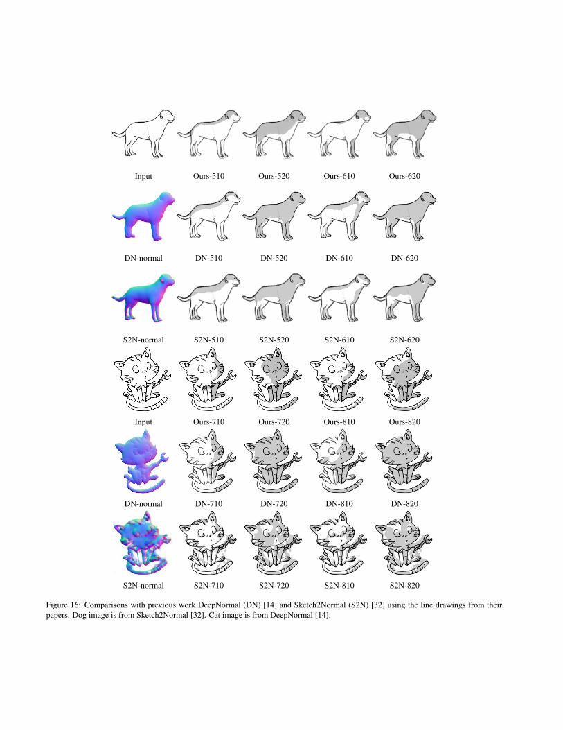
Figure 16: Comparisons with previous work DeepNormal (DN) [14] and Sketch2Normal (S2N) [32] using the line drawings from theirpapers. Dog image is from Sketch2Normal [32]. Cat image is from DeepNormal [14].





Figure 17: Comparisons with DeepNormal (DN) [14] using the line drawings and normal maps in [14]’s paper.

(a) colorized (b) lines (c) shadow - 610 (d) shadow - 710 (e) shadow - 810

(f) colorized (g) lines (h) shadow - 210 (i) shadow - 320 (j) shadow - 820

(k) colorized (l) lines (m) shadow - 220 (n) shadow - 320 (o) shadow - 710

(p) colorized (q) lines (r) shadow - 210 (s) shadow - 320 (t) shadow - 820

Figure 18: Our results using [6]’s images. [6] solves similar problems, inputting colorized images to predict the normal maps midway thengenerate the binary shadows. The colorized images (a), (f), (k), (p) are from [6]. (b), (g), (l), (q) are the lines that we subtract from thecolorized images. Our system uses (b), (g), (l), (q) as the inputs to predict the pure shadows, then composite the shadows with the colorizedimages. For each line drawing, we show our results in three lighting directions. Please refer to [6] for the their results in similar lightingdirections.

Input DN-normal S2N-normal 3D model GT-normal

Ours-120 DN-120 S2N-120 GT3D-120 GT-120

Ours-220 DN-220 S2N-220 GT3D-220 GT-220

Figure 19: Comparisons on 3D test model [8] with DeepNormal (DN) [14], Sketch2Normal (S2N) [32] and Ground Truth (GT). GT3D:rendered directly from 3D model with commercial software. GT: rendered from its normal map. All of the normal maps, including groundtruth, are rendered with the same settings as the paper (use the renderer scripts provided by DeepNormal and threshold the continuousshadings at 0.5). Along with the bunny 3D test model in paper, our shadows are most close to the ground truth.

810 210110

210 220 230

810 110 210

210 220 230

Figure 20: Examples of our continuous shadows between the discrete lighting source.

110 120 130 210 220 230

310 320 330 410 420 430

510 520 530 610 620 630

710 720 730 810 820 830

001 002

Figure 21: Evaluations of our work in all 26 directions.

110 120 130 210 220 230

310 320 330 410 420 430

510 520 530 610 620 630

710 720 730 810 820 830

001 002

Figure 22: Evaluations of our work in all 26 directions.

(a) (b) (c) (d)

Original 710 720 730 001

710+001 720+001 730+001

(f)(e)

(g) (h) (i) (j) (k)

730+001720+001710+001

Lines(l)

Figure 23: Examples of our shadowing system applying to artistic line drawing (Antoine Thomeguex, drawn by Jean Auguste DominiqueIngres. Public domain.). (a): original sketch. (b): extract lines from (a). (c)-(f): binary shadows in 710, 720, 730 and 001 lightingdirections. (g)-(i): composites of binary shadows in dual lighting directions. (j)-(l): soft shadows in dual lighting directions. The resultsshow that our shadowing system can give artists hints or a starting point to study shadows in different lighting sources.

(a) Original (b) 710 (c) (a)+(b) (d) 720 (e) (a)+(d) (f) 730 (g) (a)+(f)

(h) Lines (i) 310 (j) (a)+(h) (k) 320 (l) (a)+(j) (m) 330 (n) (a)+(l)

Figure 24: Examples of our shadowing system applying to Ukiyo-e (Kabuki Actor Segawa Kikunoj III as the Shirabyshi Hisakata Disguisedas Yamato Manzai, by Toshusai Sharaku. Public domain.). Composite our shadows with pure colorized artwork.

(a) Original (b) w/o shadows (c) Lines (d) 510 (e) 520 (f) 530

(g) 210 (h) 220 (i) 230 (j) 810 (k) 820 (l) 830

(m) 110 (n) 120 (o) 130 (p) 710 (q) 720 (r) 730

Figure 25: Examples of our shadowing system applying to poster (Jardin de Paris, Fłte de Nuit Bal, illustrated by Jules Cheret. Publicdomain.). (a): original poster. (b): remove the shadows in the human. (c): extract line drawing from (a). (d)-(r): composites our shadowsin various lighting directions with (b). Assuming the artists draw artwork with digital tools, they can rapidly try different shadows with ourshadowing system.

(a) line drawing (w/o p.) (b) (a) (w/ p.) (c) stylized (a) (w/o p.) (d) (c) (w/ p.)

(e) shadow from (a) (f) shadow from (b) (g) shadow from (c) (h) shadow from (d)

(i) line drawing (w/o p.) (j) (i) (w/ p.) (k) stylized (i) (w/o p.) (l) (k) (w/ p.)

(m) shadow from (i) (n) shadow from (j) (o) shadow from (k) (p) shadow from (l)

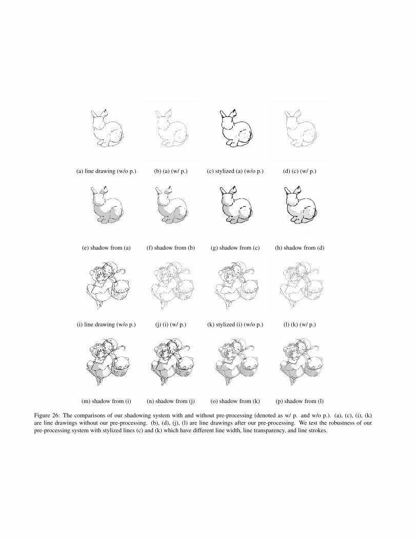
Figure 26: The comparisons of our shadowing system with and without pre-processing (denoted as w/ p. and w/o p.). (a), (c), (i), (k)are line drawings without our pre-processing. (b), (d), (j), (l) are line drawings after our pre-processing. We test the robustness of ourpre-processing system with stylized lines (c) and (k) which have different line width, line transparency, and line strokes.

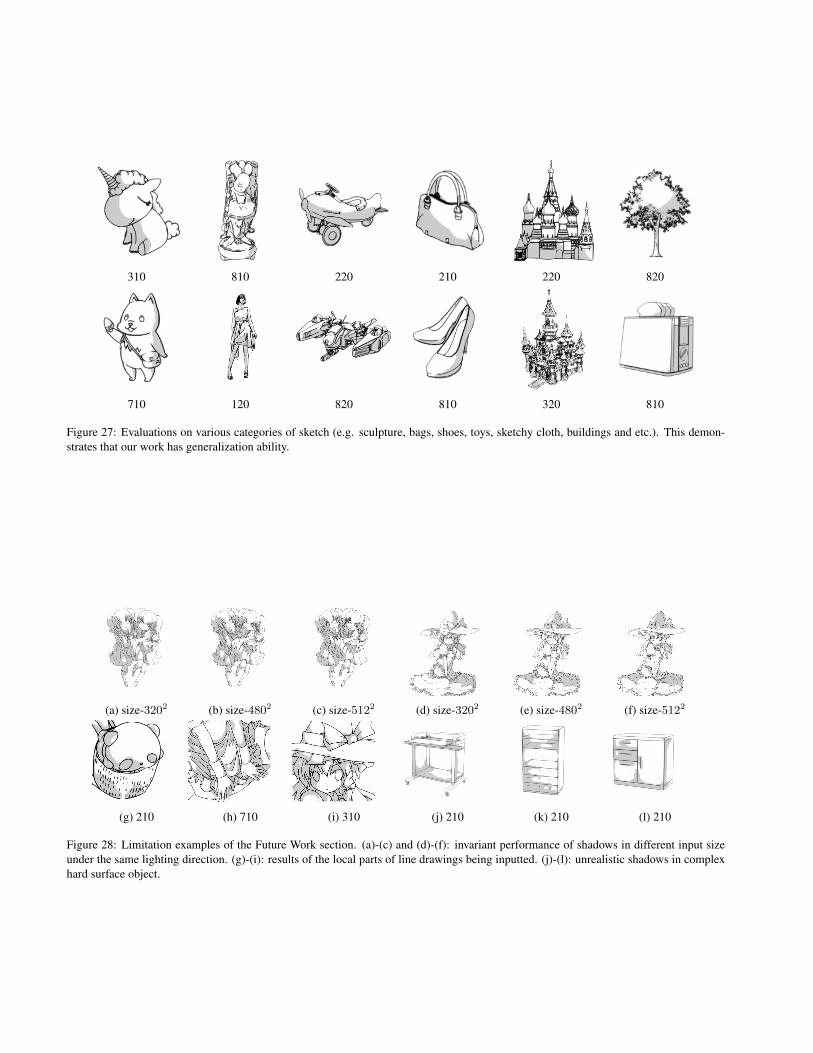
310 810 220 210 220 820

710 120 820 810 320 810

Figure 27: Evaluations on various categories of sketch (e.g. sculpture, bags, shoes, toys, sketchy cloth, buildings and etc.). This demon-strates that our work has generalization ability.

(a) size-3202 (b) size-4802 (c) size-5122 (d) size-3202 (e) size-4802 (f) size-5122

(g) 210 (h) 710 (i) 310 (j) 210 (k) 210 (l) 210

Figure 28: Limitation examples of the Future Work section. (a)-(c) and (d)-(f): invariant performance of shadows in different input sizeunder the same lighting direction. (g)-(i): results of the local parts of line drawings being inputted. (j)-(l): unrealistic shadows in complexhard surface object.

520 720

210 310

001

810

002

110

410

220 820 820

710

830

620

Sketch Sketch SketchShadow Shadow ShadowMask Mask Mask

Figure 29: Sketch/shadow/mask pairs from our dataset. Our dataset contains alpha masks for the line drawings, but we did not need to usethese masks in this paper.

learning to shadow hand-drawn sketches - arxiv · learning to shadow hand-drawn sketches qingyuan...

Documents