Learning to Localize Little Landmarks

Saurabh Singh, Derek Hoiem, David ForsythUniversity of Illinois, Urbana-Champaign

http://vision.cs.illinois.edu/projects/litland/{ss1, dhoiem, daf}@illinois.edu

Abstract

We interact everyday with tiny objects such as the doorhandle of a car or the light switch in a room. These littlelandmarks are barely visible and hard to localize in images.We describe a method to find such landmarks by finding asequence of latent landmarks, each with a prediction model.Each latent landmark predicts the next in sequence, and thelast localizes the target landmark. For example, to find thedoor handle of a car, our method learns to start with a latentlandmark near the wheel, as it is globally distinctive; subse-quent latent landmarks use the context from the earlier onesto get closer to the target. Our method is supervised solelyby the location of the little landmark and displays strongperformance on more difficult variants of established tasksand on two new tasks.

1. IntroductionThe world is full of tiny but useful objects such as the

door handle of a car or the light switch in a room. We callthese little landmarks. We interact with many little land-marks everyday, often not actively thinking about them oreven looking at them. Consider the door handle of a car(Figure 1), it is often the first thing we manipulate wheninteracting with the car. However, in an image it is barelyvisible; yet we know where it is. Automatically localizingsuch little landmarks in images is hard, as they don’t havea distinctive appearance of their own. These landmarks arelargely defined by their context. We describe a method tolocalize little landmarks by discovering informative contextsupervised solely by the location of the little landmark. Wedemonstrate the effectiveness of our approach on severaldatasets, including both new and established problems.

The target landmark may have a local appearance that issimilar to many other locations in the image. However, itmay occur in a consistent spatial configuration with somepattern, such as an object or part, that is easier to find andwould resolve the ambiguity. We refer to such a pattern asa latent landmark. The latent landmark may itself be hard

Step 1

Step 2 Step 3

Figure 1. Several objects of interest are so tiny that they barelyoccupy few pixels (top-left), yet we interact with them daily. Lo-calizing such objects in images is difficult as they do not havea distinctive local appearance. We propose a method that learnsto localize such landmarks by learning a sequence of latent land-marks. Each landmark in this sequence predicts where the nextlandmark could be found. This information is then used to predictthe next landmark and so on, until the target is found.

to localize, although easier than the target. Another latentlandmark may then help localize the earlier one, which inturn localizes the target. Our method discovers a sequenceof such landmarks, where every latent landmark helps findthe next one, with the sequence ending at the location of thetarget.

The first latent landmark in the sequence must be local-izable on its own. Each subsequent landmark must be lo-calizable given the previous landmark and predictive of thenext latent landmark or the target. Our approach has to dis-cover globally distinctive patterns to start the sequence andconditionally distinctive ones to continue it, while only be-ing supervised by the location of the target. A detection of alatent landmark includes a set of positions, typically highlyconcentrated, and a prediction of where to look next. The

training loss function specifies that each of the first latentlandmarks must predict the next latent landmark, and thelast latent landmark must predict the target location. Wetrain a deep convolutional network to learn all latent land-marks and predictions jointly. Our experiments on exist-ing CUBS200 [43] and LSP [17] datasets and newly cre-ated car door handle and light switch datasets demonstratethe effectiveness of our approach. Code and datasets areavailable on the project webpage at http://vision.cs.illinois.edu/projects/litland/.Contributions: We describe: 1) A novel and intuitiveapproach to localize little landmarks automatically. Ourmethod learns to find useful latent landmarks and corre-sponding prediction models that can be used to localizethe target; 2) A recurrent architecture using Fully Convo-lutional Networks that implements our approach; 3) A rep-resentation of spatial information particularly useful for ro-bust prediction of locations by neural networks; 4) Two newdatasets emphasizing practically important little landmarksthat are hard to find.

2. Related WorkLandmark localization has been well-studied in the do-

main of human pose estimation [45, 42, 40, 12, 33, 2, 9, 39]as well as bird part localization [24, 25, 43, 34]. Localiza-tion of larger objects has similarly been well-studied [14,15]. However, practically no work exists for localizing littlelandmarks.

Little landmarks are largely defined by their context.Thus, a successful method for localizing them will have touse this context. Use of context to improve performancehas been studied (e.g. [27, 22]). In many problems, ex-plicit contextual supervision is available. Felzenszwalb etal. [14] use contextual rescoring to improve object detec-tion performance. Singh et al. [36] use context of easylandmarks to find the harder ones, Su et al. [37] use con-text from attributes in image classification. In contrast, ourmethod has no access to explicit contextual supervision.Some methods do incorporate context implicitly e.g. Auto-Context [41], which iteratively includes information froman increasing spatial support to localize body parts. In con-trast, our method learns to find a sequence of latent land-marks that are useful for finding the target little landmarkwithout other supervised auxiliary tasks.

The work of Karlinsky et al. [19] is conceptually mostrelated to our method. They evaluate keypoint proposals tochoose an intermediate set of locations that can be used toform chains from a known landmark to a target. The targetis predicted by marginalizing over evidence from all chains.In contrast, our approach does not use keypoint proposalsand learns to find the first point in the chain as well.

Other closely related approaches are that of Alexe etal. [1] and Carreira et al. [6]. Alexe et al. learn a con-

text driven search for objects. In each step, their methodpredicts a window that is most likely to contain the ob-ject given the previous windows and the features observedat those windows. This is done by a non-parametric vot-ing scheme where the current window is matched to sev-eral windows in training images and votes are cast basedon observed offsets to target object. Carreira et al. makea spatial prediction in each step and encode it by placing agaussian at the predicted location. This is then used as a fea-ture by the next step. Similar to Alexe et al., they superviseeach step to predict the target. In addition, they constrain itto get closer to the target in comparison to previous step’sprediction. In contrast, our method does not perform anymatching with training images and does not supervise theintermediate steps with the target. Only the final step is di-rectly supervised. The latent landmarks can be anywhere inthe image as long as they are predictive of the next one inthe sequence. Further, our method is trained end-to-end.

Reinforcement learning based methods bear some sim-ilarity to our method where they also operate in steps.Caicedo et al. [5] cast object detection in a reinforcementlearning framework and learn a policy to iteratively refine abounding box for object detection, Zhang et al. [46] learnto predict a better bounding box given an initial estimate. Incomparison, our method does not have explicitly defined ac-tions or a value function. Instead, it performs a fixed-lengthsequence of intermediate steps to find the target location.

Also related are methods that discover mid-level visualelements [35, 11, 18, 38] and use them as a representationfor some task. The criterion for discovery of these elementsis often not related to the final task they are used for. Someapproaches have tried to address this by alternating betweenupdating the representation and learning for the task [29].In contrast, our method learns to find latent landmarks thatare directly useful for localizing the target and is trainableend-to-end.

Our method has similarities with attention based meth-ods that learn to look at a sequence of useful parts of theimage [3, 44, 23, 4, 26]. An important difference is that anintermediate part is constrained to be spatially predictive ofthe next one.

3. ApproachThe simplest scheme for finding a landmark looks at ev-

ery location and decides whether it is the target landmark ornot. We refer to this scheme as Detection. Training such asystem is easy: we provide direct supervision for the targetlocation. However this doesn’t work well for little land-marks because they are not strongly distinctive. Now imag-ine using a single latent landmark to predict the location ofthe target, which could be far way. We refer to this schemeas Prediction. This is hard, because we don’t have direct su-pervision for the latent landmark. Instead, the system must

Conv3(5,)5,)1,)50))

Conv2(7,)7,)1,)64))

Conv1(15,)15,)1,)48))

Pool3(3,)3,)2,)50))

Pool2(3,)3,)2,)64))

Pool1(3,)3,)2,)48))

Conv7(5,)5,)1,)50))

Conv8(5,)5,)1,)25+1))

Predic:on)

Step%1%

Conv7(5,)5,)1,)50))

Conv8(5,)5,)1,)25+1))

Predic:on)

Step%2%

Conv7(5,)5,)1,)50))

Conv8(5,)5,)1,)25+1))

Predic:on)

Step%3%

Conv4(5,)5,)1,)50))

Car)2417)

Conv5(5,)5,)1,)50)) Conv6(5,)5,)1,)50))

Figure 2. Model and Inference Overview. Our approach oper-ates in steps, where, in each step, a latent landmark (red blobsat the top, best viewed with zoom) predicts the location of thelatent landmark for the next step. This is encoded as a featuremap with radial basis kernel (blue blob) and passed as a featureto the next step. This process repeats until the last step whenthe target is localized (door handle in above). Green boxes showlayers and parameters that are shared across steps, while orange,purple and blue show step specific layers. Format for a layer islayer name(height, width, stride, num output channels).

infer where these landmarks are. Furthermore, it must learnto find these landmarks and to use them to predict where thetarget is. While this is clearly harder to learn than detection,we describe a method that is successful and outperformsDetection (§ 4.1). Note that Prediction reduces to Detectionif the latent landmark is forced to lie on the target.

Prediction is hard when the best latent landmark for atarget is itself hard to find. Here, we can generalize to asequential prediction scheme (referred to as SeqPrediction).The system uses a latent landmark to predict the location ofanother latent landmark; uses that to predict the location ofyet another latent landmark; and so on, until the final steppredicts the location of the target. Our method successfullyachieves this and outperforms Prediction (§ 4.1).

Note that another generalization that is natural but notuseful is an alternating scheme. One might estimate somemid-level pattern detectors, learn a prediction model, andthen re-estimate the detectors conditioned on the currenttarget estimates, etc. This scheme is unhelpful when thelandmark is itself hard to find. First, re-estimates tend to bepoor. Second, it is tricky to learn a sequential prediction asone would have to find conditionally distinctive patterns.

Our approach discovers latent landmarks that are directlyuseful for the localization of a target, as it is supervised only

by this objective and can be trained end-to-end. Our methodthus learns to find a sequence of latent landmarks each witha prediction model to find the next in sequence. In the fol-lowing, we first provide an overview of the model, followedby the prediction scheme, and finally the training details.

3.1. Model and Inference

Figure 2 provides an overview of the model and how it isused for the inference. Our method operates in steps whereeach step s ∈ {1, . . . , S} corresponds to a Prediction. Eachstep predicts the location of the next latent landmark usingthe image features and the prediction from the previous step.The final step predicts the location of the target landmark.To make the prediction, each step finds a latent landmark(Figure 2, red blob) and makes an offset prediction to thenext latent landmark. This prediction is encoded as a featuremap (blue blob) and passed on to the next step. Note thatthe spatial prediction scheme is of key importance for thesystem to work. We describe it in Section 3.2.

Our system uses a fully convolutional network architec-ture, sliding a network over the image to make the predic-tion at each location. In Figure 2, the green boxes indi-cate the layers with parameters shared across various steps.Other colored boxes (orange, purple and blue) show lay-ers that have step specific parameters. Note that this con-figuration of not sharing parameters for the layer that op-erates directly on features from previous step worked bet-ter than sharing all parameters and a few other alternatives(§ 5). The step specific parameters allow the features of astep to quickly adapt as estimates of underlying landmarksimprove. Our model is trained using stochastic gradient de-scent on a robust loss function. Our loss function encour-ages earlier steps to be informative for the later steps bypenalizing disagreement between the predicted and later de-tected latent landmark locations.

3.2. Prediction Scheme for a Step

Since our model is fully convolutional, images of differ-ent sizes produce feature maps of different sizes. To makea single prediction for the whole image we view the imageas a grid of locations li, i ∈ {1, . . . , L}. Each location canmake a prediction using the sliding neural network and thecombined prediction is a weighted average of these.

Each step s produces a summary estimate of the positionof the next latent landmark P (s). Each location li separatelyestimates this position as p(s)i with a confidence c(s)i . Eachp(s)i is estimated using a novel representation scheme with

several nice properties (§ 3.3). The individual predictionsare then combined as

P (s) =

L∑i=1

c(s)i p

(s)i (1)

Local&Grid&Confidences&

Local&Grid&Points&

Predicted&Offset&

Image&Grid&Confidences&

Image&Grid&Predic7ons&

Predicted&Loca7on&for&next&Landmark&

Offset&Predic7on& Predic7on&for&Step&

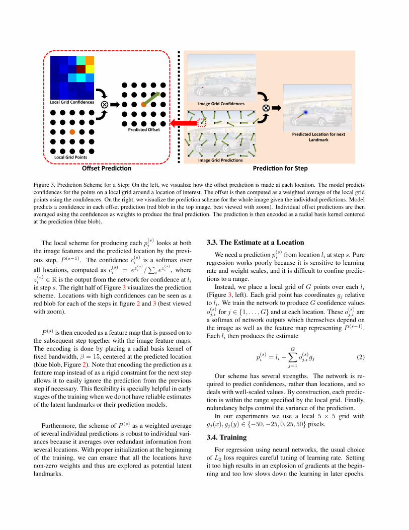
Figure 3. Prediction Scheme for a Step: On the left, we visualize how the offset prediction is made at each location. The model predictsconfidences for the points on a local grid around a location of interest. The offset is then computed as a weighted average of the local gridpoints using the confidences. On the right, we visualize the prediction scheme for the whole image given the individual predictions. Modelpredicts a confidence in each offset prediction (red blob in the top image, best viewed with zoom). Individual offset predictions are thenaveraged using the confidences as weights to produce the final prediction. The prediction is then encoded as a radial basis kernel centeredat the prediction (blue blob).

The local scheme for producing each p(s)i looks at boththe image features and the predicted location by the previ-ous step, P (s−1). The confidence c(s)i is a softmax overall locations, computed as c(s)i = ez

(s)i /

∑i ez(s)i , where

z(s)i ∈ R is the output from the network for confidence at li

in step s. The right half of Figure 3 visualizes the predictionscheme. Locations with high confidences can be seen as ared blob for each of the steps in figure 2 and 3 (best viewedwith zoom).

P (s) is then encoded as a feature map that is passed on tothe subsequent step together with the image feature maps.The encoding is done by placing a radial basis kernel offixed bandwidth, β = 15, centered at the predicted location(blue blob, Figure 2). Note that encoding the prediction as afeature map instead of as a rigid constraint for the next stepallows it to easily ignore the prediction from the previousstep if necessary. This flexibility is specially helpful in earlystages of the training when we do not have reliable estimatesof the latent landmarks or their prediction models.

Furthermore, the scheme of P (s) as a weighted averageof several individual predictions is robust to individual vari-ances because it averages over redundant information fromseveral locations. With proper initialization at the beginningof the training, we can ensure that all the locations havenon-zero weights and thus are explored as potential latentlandmarks.

3.3. The Estimate at a Location

We need a prediction p(s)i from location li at step s. Pureregression works poorly because it is sensitive to learningrate and weight scales, and it is difficult to confine predic-tions to a range.

Instead, we place a local grid of G points over each li(Figure 3, left). Each grid point has coordinates gj relativeto li. We train the network to produce G confidence valueso(s)j,i for j ∈ {1, . . . , G} and at each location. These o(s)j,i are

a softmax of network outputs which themselves depend onthe image as well as the feature map representing P (s−1).Each li then produces the estimate

p(s)i = li +

G∑j=1

o(s)j,i gj (2)

Our scheme has several strengths. The network is re-quired to predict confidences, rather than locations, and sodeals with well-scaled values. By construction, each predic-tion is within the range specified by the local grid. Finally,redundancy helps control the variance of the prediction.

In our experiments we use a local 5 × 5 grid withgj(x), gj(y) ∈ {−50,−25, 0, 25, 50} pixels.

3.4. Training

For regression using neural networks, the usual choiceof L2 loss requires careful tuning of learning rate. Settingit too high results in an explosion of gradients at the begin-ning and too low slows down the learning in later epochs.

Instead, we use Huber loss (eq. 3) for robustness.

H(x) =

{x2

2δ , if |x| < δ.

|x| − δ2 , otherwise.

(3)

For a vector x ∈ RD we define Huber loss as H(x) =∑Di=1H(xi). Robustness arises from the fact that the gradi-

ents are exactly one for large loss values (|x| > δ), and lessthan one for smaller values ensuring stable gradient magni-tudes. We use δ = 1.

Assume that we know the regression target y(s)∗ for steps. Then, given the prediction P (s), we define the loss forstep s as following

L(s) = H(P (s) − y(s)∗ ) + γ

L∑i=1

c(s)i H(p

(s)i − y

(s)∗ ) (4)

The first term enforces that the prediction p(s) coincideswith the target y(s)∗ . The second term enforces that the in-dividual predictions for each location also fall on the target,but the individual losses are weighted by their contributionto the final prediction. We found that the use of this termwith a small value of γ = 0.1 consistently leads to solu-tions that generalize better.

The regression target for the final step S is the knownground truth location y∗. But we do not have supervisionfor the intermediate steps. We would like our step s to pre-dict the location of the latent landmark of the next step s+1.Note that the latent landmark for the next step is consideredto be the set of locations in the image that the model consid-ers to be predictive and therefore assigns high confidencesc(s+1)i . We set y(s)∗ =

∑Li=1 c

(s+1)i li, i.e. as the centroid

of locations with confidence weights c(s+1)i in the next step.

This setting encourages the prediction from step s to coin-cide with the locations that are predictive in next step.

We define the full loss for a given sample as a weightedsum of the losses from individual steps as following

L =

S∑s=1

λsL(s) +R(θ) (5)

We use λs = 0.1, except for the final step S where λS = 1,assigning more weight to the target prediction. R(θ) isa regularizer for the parameters of the network. We useL2 regularization of network weights with a multiplier of0.005.Training Details: We train our model through back-propagation using stochastic gradient descent with mo-mentum. The errors are back-propagated across the stepsthrough the radial basis kernel based feature encoding of thelatent landmark prediction in each step. Since our model isrecurrent, we found that the use of gradient scaling makes

Normalized Distance →

0 0.02 0.04 0.06 0.08 0.1

DetectionRate

→

0

0.2

0.4

0.6

0.8

1

Img Reg

Det

Pred

Pred 2

Pred 3

Figure 4. Our method localizes car door handles very accurately.Pred 3, the three step SeqPrediction scheme, outperforms the otherschemes. Det, Pred and Pred 2 are Detection, Prediction and twostep SeqPrediction schemes respectively. Img Reg is a baselinethat replaces classification layer by a regression layer in the VGG-M model. Table 1 reports detection rates at a fixed normalizeddistance of 0.02.

Seq. Prediction

Method Img Reg Det Pred Pred 2 Pred 3

Det. Rate 6.1 19.2 54.3 63.3 74.4Table 1. Detection rates for the Car Door Handle Dataset at thefixed normalized distance of 0.02. The three step scheme (Pred3) performs significantly better than the alternatives. Refer to Fig-ure 4 for more details.

the optimization better behaved [30]. We do this by scalingthe gradients with combined L2 norm more than 1000, backdown to 1000 for all filters of each layer individually. Weinitialize the weights using the method suggested by Glo-rot et al. [16].

We augment the datasets by including left-right flips aswell as random crops near the border. The images are scaledto make the longest side 500 pixels.

4. ExperimentsWe present two new datasets: The Light Switch Dataset

(LSD) and the Car Door Handle Dataset (CDHD) that em-phasize practically important and hard to find little land-marks. Further, we evaluate our method on more difficultvariants of two established tasks: 1) beak localization onthe Caltech UCSD Birds Dataset (CUBS); 2) wrist localiza-tion on the Leeds Sports Dataset (LSP). Note that we referto the three step SeqPrediction as Ours in the following un-less specified otherwise .Evaluation Metric: We adopt the generally accepted met-

Normalized Distance →

0 0.2 0.4 0.6 0.8 1

DetectionRate

→

0

0.1

0.2

0.3

0.4

0.5

0.6

Img Reg

Det

Pred

Pred 2

Pred 3

Figure 5. Our method localizes light switches relatively well incomparison to the baselines. The baselines are the same as theones for Car Door Handle dataset. Table 2 reports detection ratesat a fixed normalized distance of 0.5.

ric of plotting detection rate against normalized distancefrom ground truth for all datasets except CUBS, where PCPis used. Normalization is based on torso height for LSP, carbounding box height for CDHD, and switch board heightfor LSD. For CUBS we report PCP as used in [24]. It iscomputed as detection rate for an error radius defined as1.5 × σhuman, where σhuman is the standard deviation ofthe human annotations.

4.1. Car Door Handle Dataset

Our method finds car door handles very accurately (Fig-ure 4 and 7 and Table 1), with superior performance tovarious baselines. Det is the Detection method, Pred isthe Prediction method and Pred 2 and Pred 3 are two andthree step SeqPrediction methods respectively (§ 3). Useof Prediction instead of Detection gives considerable per-formance improvement, while SeqPrediction provides ad-ditional improvement. Img Reg is a baseline implementedby taking the VGG-M model [7] that was pre-trained onImageNet [10], removing the top classification layer andreplacing it by a 2D regression layer. The learning ratefor all the layers was set to 0.1 times the learning rate λrfor the regression layer. The model performed best witha learning rate λr = 0.01, chosen by trying values in{0.1, 0.01, 0.001}. We noticed that the baseline general-ized poorly in all the experiments. This is likely due toa combination of VGG-M model being relatively large incomparison to the dataset size, task being regression insteadof classification and hyper-parameter range explored beingsuboptimal.Dataset details: To collect a dataset with car door handles,4150 images of the Stanford Cars dataset for fine grained

Seq. Prediction

Method Img Reg Det Pred Pred 2 Pred 3

Det. Rate 1.5 41.0 44.5 47.5 51.0Table 2. Detection rates for the Light Switch Dataset at the fixednormalized distance of 0.5. Again, the three step scheme performsbetter than alternatives.

Method PCP

Liu et al. [24] 49.0Liu et al. [25] 61.2Shih et al. [34] 51.8Ours 64.1

Table 3. Our method outperforms several state of the art methodsfor localizing beaks on the Caltech UCSD Birds Dataset. Note thatthis comparison is biased against our method; others are trainedwith all landmarks while ours is supervised only by beak.

categorization [21] were annotated. Annotators were askedto annotate the front door handle of the visible side. Thehandle was marked as hidden for frontal views of the carwhen it was not visible. We use the training and test split ofthe original dataset.

4.2. Light Switch Dataset

Our method finds light switches with reasonable accu-racy (Figure 5 and 7 and Table 2). Again, the three stepscheme performs better than the alternatives. The baselinesare the same as the ones for the Car Door Handle dataset.Img Reg baseline again generalizes poorly with LSD beingsignificantly smaller than CDHD.Dataset details: With the aim of building a challenging sin-gle landmark localization problem, we collected the LightSwitch Dataset (LSD) with 822 annotated images (622train, 200 test). Annotators were asked to mark the middlepoints of the top and bottom edge of the switch board. Thelocation of the light switch is approximated as the mean ofthese. These two points also provide approximate scale in-formation used for normalization in evaluation. This datasetis significantly harder than the Car Door Handles dataset ascontext around light switches exhibits significant variationin appearance and scale.

4.3. Caltech UCSD Birds Dataset - Beaks

Caltech-UCSD Birds 200 (2011) dataset (CUBS200) [43] contains 5994 training and 5794 testing imageswith 15 landmarks for birds. We evaluate our approach onthe task of localizing beak as the target landmark. We chosebeak because it is one of the hardest landmarks and severalstate of the art approaches do not perform well on this. Weused the provided train and test splits for the dataset.

Our method, while having access only to the beak lo-

0 0.05 0.1 0.15 0.20

0.1

0.2

0.3

0.4

0.5

0.6

0.7

Normalized Distance→

Det

ectio

nR

ate→

Chen et al. [8]Pishchulin et al. [31]Ouyang et al. [28]Ramakrishna et al. [32]Kiefel et al. [20]Ours

Figure 6. Our method, while supervised only by the location ofleft wrist, performs competitively against several state of the artmethods for localizing the left wrist landmark on the Leeds SportsDataset.

cation during training (all other methods are trained usingother landmarks as well), outperforms several state of theart methods (Table 3).

4.4. Leeds Sports Dataset - Left Wrist

Leeds Sports Dataset (LSP) [17] contains 1000 trainingand 1000 testing images of humans in difficult poses with14 landmarks. We choose left wrist as the target landmarkas wrists are known to be difficult to localize. We use theObserver Centric (OC) annotations [13] and work with pro-vided training/test splits.

Our method (Figure 6) performs competitively with sev-eral recent works all of which train their method using otherlandmarks.

5. Discussion

Figure 7 shows some qualitative results for variousdatasets. First thing to note is the pattern in the locationsof the latent landmarks for each of the datasets. For cars,the system tends to find the wheel as the first latent land-mark and then moves towards the door handle in subsequentsteps. For light switches it relies on finding the edge of thedoor first. For birds, the first landmark tends to be on theneck, followed by one near the eye and the last tends tobe outside at the curve of neck and beak. It is remarkablethat these patterns emerge solely from the supervision ofthe target landmark. Also, note that these patterns are notrigid; they adapt to the image evidence. This is primarilydue to the fact that our method does not impose any hardconstraints. Later steps can choose to ignore the evidence

from the earlier steps. This property allows our model tobe trained effectively, especially in the beginning when thelatent landmarks and their prediction models are not known.

Our method highlights the trade-off inherent in parts vs.larger template. Parts assume structure, reducing parame-ters and variance in their estimation. While larger templatessupport richer models, but with more parameters resultingin larger variance.

We explored two other architectures for propagating in-formation from one step to the next and found that the cur-rent scheme performs the best in terms of the final perfor-mance. In the first scheme, step-specific weights were at thetop instead of at the bottom of the recurrent portion of ourmodel (Figure 2, middle block). In the second scheme, in-stead of passing the encoded prediction as a feature, it wasused as a prior to modulate the location confidences of thenext step.

6. ConclusionWe described a method to localize little landmarks by

finding a sequence of latent landmarks and their predic-tion models. We demonstrated strong performance of ourmethod on harder variants of several existing and new tasks.The success of our approach arises from the spatial predic-tion scheme and the encoding of information from one stepto be used by the next. A novel and well behaved localestimation model coupled with a robust loss aids training.Promising future directions include localizing multiple tar-gets, generalizing sequence of latent landmarks to directedacyclic graphs of latent landmarks, and accumulating all theinformation from previous steps to be used as features forthe next step.

References[1] B. Alexe, N. Heess, Y. W. Teh, and V. Ferrari. Searching for

objects driven by context. In Advances in Neural InformationProcessing Systems, pages 881–889, 2012. 2

[2] M. Andriluka, S. Roth, and B. Schiele. Pictorial structuresrevisited: People detection and articulated pose estimation.In CVPR, 2009. 2

[3] J. Ba, V. Mnih, and K. Kavukcuoglu. Multiple object recog-nition with visual attention. arXiv preprint arXiv:1412.7755,2014. 2

[4] D. Bahdanau, K. Cho, and Y. Bengio. Neural machinetranslation by jointly learning to align and translate. arXivpreprint arXiv:1409.0473, 2014. 2

[5] J. Caicedo and S. Lazebnik. Semantic guidance of visualattention for localizing objects in scenes. In ICCV, 2015. 2

[6] J. Carreira, P. Agrawal, K. Fragkiadaki, and J. Malik. Humanpose estimation with iterative error feedback. arXiv preprintarXiv:1507.06550, 2015. 2

[7] K. Chatfield, K. Simonyan, A. Vedaldi, and A. Zisserman.Return of the devil in the details: Delving deep into convo-

12

3

1 2

312

3

1 2

3

1

2

3

1

2

3

1

2

3

12

3

12

3

1 2

3

12

3

12

3

12

3

12

3

1

2

3

12

3

1

2

31

2

3

1

2

3

1

2

3

1

2

3

1

2

3

1

2

3

1

2

31

2

3

Figure 7. Qualitative results for the Car Door Handle Dataset (top two rows), Light Switch Dataset (middle two rows) and the CaltechUCSD Birds Dataset (last two rows) (best viewed with zoom). Ground truth locations are shown as a black triangle. Step 1, Step 2 andStep 3 are color coded as Red, Green and Blue respectively. Colored blobs show the locations of the latent landmarks for each step. Solidcircles with numbers show the predicted location of the next latent landmark by each step. Dotted circles show the bandwidth of the radialbasis kernel used to encode the predictions. Note the patterns in the locations of the latent landmarks. For cars, the first latent landmarktends to be on the wheel and later ones get closer to the door handle. For light switches it relies on finding the edge of the door first. Forbirds, the first landmark tends to be on the neck, followed by one near the eye and the last tends to be outside at the curve neck and beak.Rightmost column shows failure/interesting cases for each dataset (red border). It is evident that the latent landmarks tend to be close tothe prediction from the previous step, though they are not constrained to do so (bottom right bird image). Typical failure modes includeclutter, circumstantial contextual signal (door frame) and rarer examples (e.g. flying bird).

lutional nets. In British Machine Vision Conference, 2014.6

[8] X. Chen and A. Yuille. Articulated pose estimation by agraphical model with image dependent pairwise relations.arXiv preprint arXiv:1407.3399, 2014. 7

[9] M. Dantone, J. Gall, C. Leistner, and L. van Gool. Humanpose estimation from still images using body parts dependentjoint regressors. In CVPR. IEEE, 2013. to appear. 2

[10] J. Deng, W. Dong, R. Socher, L.-J. Li, K. Li, and L. Fei-Fei. Imagenet: A large-scale hierarchical image database. InCVPR, 2009. 6

[11] C. Doersch, S. Singh, A. Gupta, J. Sivic, and A. A. Efros.What makes paris look like paris? ACM Transactions onGraphics (SIGGRAPH), 31(4), 2012. 2

[12] M. Eichner and V. Ferrari. Better appearance models forpictorial structures. In ICCV, 2009. 2

[13] M. Eichner and V. Ferrari. Appearance sharing for collectivehuman pose estimation. In ACCV, 2012. 7

[14] P. Felzenszwalb, R. Girshick, D. McAllester, and D. Ra-manan. Object detection with discriminatively trained part-based models. IEEE Trans. on Pattern Analysis and MachineIntelligence, 2010. 2

[15] R. Girshick, J. Donahue, T. Darrell, and J. Malik. Rich fea-ture hierarchies for accurate object detection a nd semanticsegmentation. In CVPR. IEEE, 2014. 2

[16] X. Glorot and Y. Bengio. Understanding the difficulty oftraining deep feedforward neural networks. In Internationalconference on artificial intelligence and statistics, pages249–256, 2010. 5

[17] S. Johnson and M. Everingham. Clustered pose and nonlin-ear appearance models for human pose estimation. In BMVC,2010. doi:10.5244/C.24.12. 2, 7

[18] M. Juneja, A. Vedaldi, C. Jawahar, and A. Zisserman. Blocksthat shout: Distinctive parts for scene classification. InCVPR, 2013. 2

[19] L. Karlinsky, M. Dinerstein, D. Harari, and S. Ullman. Thechains model for detecting parts by their context. In CVPR,pages 25–32, 2010. 2

[20] M. Kiefel and P. V. Gehler. Human pose estimation withfields of parts. In ECCV. Springer, 2014. 7

[21] J. Krause, M. Stark, J. Deng, and L. Fei-Fei. 3d object repre-sentations for fine-grained categorization. In ICCVW, 2013.6

[22] S. Kumar and M. Hebert. A hierarchical field framework forunified context-based classification. In ICCV, 2005. 2

[23] H. Larochelle and G. E. Hinton. Learning to combine fovealglimpses with a third-order boltzmann machine. In NIPS,pages 1243–1251, 2010. 2

[24] J. Liu and P. N. Belhumeur. Bird part localization usingexemplar-based models with enforced pose and subcategoryconsistency. In ICCV, 2013. 2, 6

[25] J. Liu, Y. Li, and P. N. Belhumeur. Part-pair representationfor part localization. In ECCV 2014, 2014. 2, 6

[26] V. Mnih, N. Heess, A. Graves, et al. Recurrent models ofvisual attention. In NIPS, pages 2204–2212, 2014. 2

[27] K. Murphy, A. Torralba, W. Freeman, et al. Using the forestto see the trees: a graphical model relating features, objects

and scenes. Advances in neural information processing sys-tems, 2003. 2

[28] W. Ouyang, X. Chu, and X. Wang. Multi-source deep learn-ing for human pose estimation. In CVPR. IEEE, 2014. 7

[29] S. N. Parizi, A. Vedaldi, A. Zisserman, and P. Felzenszwalb.Automatic discovery and optimization of parts for imageclassification. ICLR, 2014. 2

[30] R. Pascanu, T. Mikolov, and Y. Bengio. On the diffi-culty of training recurrent neural networks. arXiv preprintarXiv:1211.5063, 2012. 5

[31] L. Pishchulin, M. Andriluka, P. Gehler, and B. Schiele.Strong appearance and expressive spatial models for humanpose estimation. In ICCV, pages 3487–3494. IEEE, 2013. 7

[32] V. Ramakrishna, D. Munoz, M. Hebert, J. A. Bagnell, andY. Sheikh. Pose machines: Articulated pose estimation viainference machines. In ECCV, 2014. 7

[33] B. Sapp, A. Toshev, and B. Taskar. Cascaded models forarticulated pose estimation. In ECCV, 2010. 2

[34] K. J. Shih, A. Mallya, S. Singh, and D. Hoiem. Part localiza-tion using multi-proposal consensus for fine-grained catego-rization. arXiv preprint arXiv:1507.06332, 2015. 2, 6

[35] S. Singh, A. Gupta, and A. A. Efros. Unsupervised discoveryof mid-level discriminative patches. In ECCV, 2012. 2

[36] S. Singh, D. Hoiem, and D. Forsyth. Learning a sequen-tial search for landmarks. In Computer Vision and PatternRecognition, 2015. 2

[37] Y. Su and F. Jurie. Improving image classification using se-mantic attributes. International journal of computer vision,100(1):59–77, 2012. 2

[38] J. Sun and J. Ponce. Learning discriminative part detectorsfor image classification and cosegmentation. In InternationalConference on Computer Vision, 2013. 2

[39] A. Toshev and C. Szegedy. Deeppose: Human poseestimation via deep neural networks. arXiv preprintarXiv:1312.4659, 2013. 2

[40] D. Tran and D. Forsyth. Improved human parsing with a fullrelational model. In ECCV, 2010. 2

[41] Z. Tu and X. Bai. Auto-context and its application to high-level vision tasks and 3d brain image segmentation. PAMI,32(10):1744–1757, 2010. 2

[42] Y. Wang, D. Tran, and Z. Liao. Learning hierarchical pose-lets for human parsing. In CVPR, 2011. 2

[43] P. Welinder, S. Branson, T. Mita, C. Wah, F. Schroff, S. Be-longie, and P. Perona. Caltech-UCSD Birds 200. TechnicalReport CNS-TR-2010-001, California Institute of Technol-ogy, 2010. 2, 6

[44] K. Xu, J. Ba, R. Kiros, A. Courville, R. Salakhutdinov,R. Zemel, and Y. Bengio. Show, attend and tell: Neural im-age caption generation with visual attention. arXiv preprintarXiv:1502.03044, 2015. 2

[45] Y. Yang and D. Ramanan. Articulated human detection withflexible mixtures of parts. PAMI, 2013. 2

[46] Y. Zhang, K. Sohn, R. Villegas, G. Pan, and H. Lee. Im-proving object detection with deep convolutional networksvia bayesian optimization and structured prediction. arXivpreprint arXiv:1504.03293, 2015. 2