learning to coordinate: a study in retail gasoline
TRANSCRIPT

American Economic Review 2019, 109(2): 591–619 https://doi.org/10.1257/aer.20170116
591
Learning to Coordinate: A Study in Retail Gasoline†
By David P. Byrne and Nicolas de Roos*
This paper studies equilibrium selection in the retail gasoline industry. We exploit a unique dataset that contains the universe of station-level prices for an urban market for 15 years, and that encompasses a coordinated equilibrium transition mid-sample. We uncover a gradual, three-year equilibrium transition, whereby domi-nant firms use price leadership and price experiments to create focal points that coordinate market prices, soften price competition, and enhance retail margins. Our results inform the theory of collusion, with particular relevance to the initiation of collusion and equilib-rium selection. We also highlight new insights into merger policy and collusion detection strategies. (JEL G34, L12, L13, L71, L81, Q35)
Despite an extensive and influential research agenda on collusion that dates back to Stigler (1964), a fundamental question remains to be explored: how is collu-sion initiated? There are at least two reasons for this: one theoretical, and the other empirical.
Theoretically, the challenge for any model of collusion that incorporates collu-sion initiation is the complexity of collusive agreements. At a minimum, an agree-ment must stipulate when and how high to raise prices, who initiates price increases, and how quickly rivals must follow. In addition, an agreement must also specify how firms should respond to demand and cost fluctuations, what constitutes a violation of an agreement, how violations are detected and verified, and what actions to take if a violation occurs. Further, successful collusion requires a mutual understanding among firms with regard to these elements of an agreement (Harrington 2017).
* Byrne: Department of Economics, University of Melbourne, 111 Barry Street, VIC 3010, Australia (email: [email protected]); de Roos: School of Economics, University of Sydney, Merewether Building H04, NSW 2006, Australia (email: [email protected]). This paper was accepted to the AER under the guidance of Penny Goldberg, Coeditor. Two anonymous referees provided comments and suggestions that sub-stantially improved the paper. We also received valuable feedback from Victor Aguirregabiria, John Asker, Ralph Bayer, Colin Camerer, Colin Cameron, Jeff Church, Joe Harrington, Jean-François Houde, Simon Loertscher, Leslie Marx, Wallace Mullin, Charlie Plott, David Rahman, Duncan Searle, Matthew Shum, Vladimir Smirnov, Michelle Sovinsky, and Tom Wilkening. Seminar participants at the 2016 FTC Microeconomics Conference, 2016 Econometric Society Australasian Meetings, UC Davis, Caltech, U. Calgary, NUS, U. Melbourne, U. Adelaide, U. Auckland, Monash, QUT, UTS, Mannheim, the Australian Competition and Consumer Commission, and the Competition Bureau of Canada also provided comments and suggestions. Jia Sheen Nah, Daniel Tiong, and Peng Xue provided excellent research assistance. Financial support from The Samuel and June Hordern Endowment is gratefully acknowledged. The views expressed herein are solely those of the authors. Any errors or omissions are our own. The authors declare that they have no relevant or material financial interests that relate to the research described in this paper.
† Go to https://doi.org/10.1257/aer.20170116 to visit the article page for additional materials and author disclosure statement(s).

592 THE AMERICAN ECONOMIC REVIEW FEBRUARY 2019
It is hard to imagine how firms could arrive at such a mutual understanding without explicit communication. As such, theories of collusion presume collusive agreements are initiated through explicit communication, or remain agnostic as to how such an understanding emerges. Indeed, as Green, Marshall, and Marx (2015) conclude in a recent overview of the literature on collusion, while much is known in theory about how collusive agreements are implemented, little is known about how they are initiated.
Adding to these challenges is a lack of evidence to inform a theory of collusion initiation. Empirical research on collusion draws heavily on case studies of cartels engaged in explicit collusion.1 Such cases do not, however, reveal the mechanisms through which collusion emerges. While a separate body of empirical research reveals the pervasiveness of tacit collusion and coordinated effects,2 this research focuses on the presence of collusion at a point in time, not how it originates. Absent explicit communication, how do firms develop a mutual understanding of coordi-nated strategies to increase profit margins?
This paper informs this question by providing a unique empirical analysis of equilibrium selection in the retail gasoline industry. We analyze a novel dataset that contains the universe of station-level prices from an urban market for 15 years, from 2001 to 2015. The granularity of these data, combined with the fact that they encom-pass a coordinated, profit-enhancing equilibrium transition mid-sample, offers a unique opportunity to study the evolution of oligopoly pricing, coordination, and conduct.
In the gradual, three-year equilibrium transition that we uncover, dominant firms use price leadership to create focal points that facilitate price coordination and enhance profit margins.3 Further, we find that price leaders use price experiments to test rivals’ willingness to coordinate, to signal their intentions, and to create a mutual understanding of a coordinated pricing strategy among rivals.
The completeness of our data permits a purely descriptive analysis to establish these empirical results. We describe the dataset in Section I. In Section II, we show the emergence of pricing focal points in April 2009, and a subsequent permanent and substantial increase in firms’ margins starting in March 2010. Section III shows how dominant firms use price leadership and price experiments over a three-year period to transition the market to a stable focal point equilibrium between April 2009 and August 2012. Section IV examines how firms leverage the focal points to steadily increase their profit margins over time.
Our study concludes in Section V. Here, we relate our empirical results to the theory of collusion in economics, and ongoing debates in law about the definition of tacit communication and the legality of coordinated effects. We also offer new
1 See, for example, Igami and Sugaya (2018), Chilet (2018), Clark and Houde (2013), Asker (2010), Röller and Steen (2006), or Genesove and Mullin (2001). Levenstein and Suslow (2006) provide an extensive overview of the cartels literature.
2 Examples include Kawai and Nakabayashi (2018) (procurement), Miller and Weinberg (2017) (horizontal mergers), Lewis (2015) and Knittel and Stango (2003) (focal points), Lewis (2012) and Wang (2009) (price lead-ership), Ciliberto and Williams (2014) and Busse (2000) (multi-market contact), Cramton and Schwartz (2000) (bid signaling), and Borenstein and Shepard (1996) and Slade (1992) (demand fluctuations and price wars). There is also a large literature in antitrust law on tacit collusion and coordinated effects; see Kaplow (2013) for a review.
3 See Schelling (1960) and Bain (1968) for early references on the roles of focal points and price leadership in facilitating tacit coordination in oligopoly.

593BYRNE AND DE ROOS: LEARNING TO COORDINATEVOL. 109 NO. 2
insights from our study into merger policy and collusion detection strategies in data-rich environments.
I. The Market and Data
Our research context is Perth, Western Australia, a city of 1.7 million people. Like many cities worldwide, Perth has a concentrated retail gasoline market. Four major oil companies dominate refinement, importation, and distribution of fuel: BP, Caltex, Mobil, and Shell. Moreover, the oil majors directly or indirectly exert control over day-to-day pricing across their retail gasoline station networks. Two nationally dominant supermarket chains, Coles and Woolworths, also compete in the market and directly set their stations’ retail prices.4
From 2005 to 2015, BP is the largest retailer in the market, operating an average of 22 percent of stations year to year. Caltex, Woolworths, and Coles are the three next largest retailers. They operate 16 percent, 14 percent, and 16 percent of stations, respectively. The remaining 32 percent of stations are largely owned and operated by independent retailers. These station shares are stable between 2005 and 2015.5
Fuelwatch.—The market has a price transparency program called Fuelwatch. It was introduced by the state government on January 3, 2001. The program requires gasoline retailers to submit, via CSV web uploads, all of their next day’s station-level prices to the government each day before 2 pm. When stations open at 6 am the next day, they are required by law to post the submitted prices from the previous day. Prices are then fixed at these levels for 24 hours.
Using these station-level price data, the government posts today’s prices online for every gasoline station in the market. In addition, starting at 2:30 pm each day, the government posts tomorrow’s prices online for all stations.6 In this way, Fuelwatch aims to reduce consumers’ costs of searching for gasoline prices. However, in Byrne and de Roos (2018), we estimate that 10 to 15 percent of shoppers actively use the Website each day. Demand-side search frictions likely remain.
Fuelwatch has important implications for our empirical analysis of price leader-ship and focal point formation. The program’s design implies that (i) retail competi-tion occurs at daily frequencies; (ii) retailers set prices simultaneously each day; and (iii) retailers can perfectly monitor each other’s prices over time. In addition, retail-ers face common daily cost shocks as fluctuations in crude oil prices and exchange rates are transmitted to local wholesale gasoline prices. Further, aside from sta-tion location, retail gasoline is reasonably characterized as a homogeneous prod-uct. These various features of the market imply that our setting maps well into the benchmark repeated games model of collusion with simultaneous price competition and perfect monitoring.
4 Coles and Woolworths have 37 percent and 40 percent market shares in the supermarket sector, respectively (NARGA 2010). IGA and Aldi are the next largest retailers, with 15 percent and 3 percent shares, respectively, and do not sell gasoline.
5 Details are in online Appendix A.1.6 Online Appendix A.3 depicts the Fuelwatch website. From our discussions with the Fuelwatch team, we
understand that compliance with the Fuelwatch program is nearly perfect.

594 THE AMERICAN ECONOMIC REVIEW FEBRUARY 2019
Other Institutional Details.—Our analysis focuses on an equilibrium transition commencing in 2009. Between 2009 and 2015 there are no major changes in market structure, demand, or policy.7
A. Data
We collected the universe of daily station-level price observations from January 3, 2001 to January 1, 2015 from www.fuelwatch.gov.au.8 In total, we have an unbal-anced panel of 1,613,163 retail gasoline price observations for regular unleaded fuel across 687 stations. Prices are in terms of cents per liter (cpl). Importantly, each retail price is linked to a station and brand. This allows us to track station entry and exit, and the evolution of retailers’ station networks over time.
We match the daily terminal gate price (TGP) for wholesale gasoline to these retail price data. The TGP is a local spot price for wholesale gasoline which includes a margin for upstream suppliers. We use the lowest TGP each day across Perth’s six gasoline terminals as a proxy for stations’ marginal costs.9 Daily TGP data are available from the Fuelwatch website from January 19, 2002 onwards.
II. Fifteen Years of Retail Pricing
Retail prices exhibit an asymmetric cycle throughout our sample period.10 Figure 1 depicts an example cycle between January and April 2011. The figure plots average daily station-level retail prices for the four major firms and an independent firm, Gull. Retail prices infrequently jump (the relenting phase), with daily price cutting between price jumps (the undercutting phase). The figure also shows how the level of the cycle trends with wholesale fuel costs (TGP).
For our analysis of retail pricing and coordination, it is helpful to define price jumps and cycles at the station and market levels.
DEFINITION 1:
(i) A station-level price jump occurs at station i on date t if Δ p it ≥ 6 cpl , where p it is the retail price and Δ p it = p it − p it−1 .
(ii) A station-level price cycle starts at station i on date t if Δ p it ≥ 6 cpl . This is denoted as “day 1” of the station-level cycle. Days 2, 3, 4, … of the
7 See online Appendix A for an extensive discussion of various other institutional details. These include the history of retailer entry and exit; the evolution of market shares; contracts between wholesalers and retailers, gas-oline price discounts tied to grocery purchases; daily gasoline demand fluctuations; the structure of the Fuelwatch price transparency program and website; and all other aggregate demand, cost, and policy shocks.
8 We focus on the 2001 to 2014 period because of 3 supply-side shocks: (i) Woolworths completing a sale of 45 percent of its stations to Caltex in February 2015, (ii) Chevron selling its majority ownership share in Caltex Australia in March 2015, and (iii) BP and Woolworths forming a joint venture in August 2017. Excluding 2015 to 2017 is inconsequential for our analysis of price leadership, focal point formation, and equilibrium transition, which spans 2009 to 2012.
9 We abstract from time-invariant marginal cost components such as quantity discounts and shipping costs, as retailer-specific cost data are unavailable. In using the TGP to measure profit margins, we follow previous studies (e.g., Borenstein and Shepard 1996, Lewis 2012).
10 Retail gasoline price cycles exist in the United States, Canada, Australia, and Europe (Eckert 2013).

595BYRNE AND DE ROOS: LEARNING TO COORDINATEVOL. 109 NO. 2
station-level cycle correspond to the undercutting phase, which continues until the next station-level price jump occurs and a new cycle starts. Station-level cycle length is the number of days between station-level price jumps.
(iii) A market price jump occurs on date t if media n t (Δ p it ) ≥ 6 cpl , where media n t (Δ p it ) is the median of Δ p it across all stations on date t .
(iv) A market cycle commences on date t if media n t (Δ p it ) ≥ 6 cpl . This is denoted as “day 1” of the market cycle. Days 2, 3, 4, … of the market cycle correspond to the undercutting phase, which continues until the next market price jump occurs and a new cycle begins. Market cycle length is the number of days between market price jumps.
(v) Station i is a cycling station in year y if Δ p it ≥ 6 cpl at least 15 times in year y .
Part (v) acknowledges that not all stations in the market are cycling. However, the majority of stations exhibit price cycles: 507 of the 687 stations are cycling in at least 1 sample year. For the remainder of the paper, we focus only on the pricing behavior of stations engaged in price cycles.11 Our results are robust to variations in the definitions of station-level and market price jumps and cycles.
11 Online Appendix E.1 provides a comparison of cycling and non-cycling stations. We find the share of cycling stations in the market is stable over time. Firm type is the main predictor of a station’s cycling status. On average, 39 percent of small independent stations engage in cycles and 76 percent of oil major and supermarket stations engage in cycles year to year. After 2010, these figures for cycle participation are 38 percent for independents and
Figure 1. Retail Price Cycles
120
130
140
150
Avg
. sta
tion-
leve
l pric
e, te
rmin
al g
ate
pric
e (c
pl)
01 Jan 2011 01 Feb 2011 01 Mar 2011 01 Apr 2011
Date
BP Caltex Woolworths Coles Gull Terminal gate price
596 THE AMERICAN ECONOMIC REVIEW FEBRUARY 2019
Among cycling stations, the average station-level daily price jump is 11.06 cpl (SD = 2.68), while the average daily price cut during the undercutting phase is −1.28 cpl (SD = 1.84). The average retail margin is 14.05 cpl (SD = 3.76) on price jump days, and 6.06 cpl (SD = 4.89) on price cut days. Station-level cycle length is 8.8 days on average (SD = 4.4).
A. Two Focal Points Emerge
The degree to which stations coordinate on the timing and magnitude of price jumps and cuts evolves dramatically over our sample period. Figure 2 shows the evolution of the timing of market price jumps. Panel A presents a scatter plot where the horizontal axis represents the calendar date, and the vertical axis contains seven dummy variables, one for each day of the week, that equal one if a market price jump occurs on that particular day of the week. Prior to April 2009, price jumps are dispersed throughout the week. After April 2009, the vast majority of market price jumps occur on Thursdays; this is especially the case a year later starting in April 2010. This reveals our first focal point: Thursday jumps.12
Panel B of Figure 2 depicts a corresponding collapse in cycle length dispersion starting in April 2009. The figure plots the average station-level cycle length for each month and firm across BP, Caltex, Woolworths, Coles, and Gull stations. Prior to April 2009, average cycle length varies considerably over time, ranging from 7 to 35 days. However, when Thursday jumps first emerge as a focal point in April 2009, average station-level cycle length converges to seven days for all firms, and remains stable thereafter.
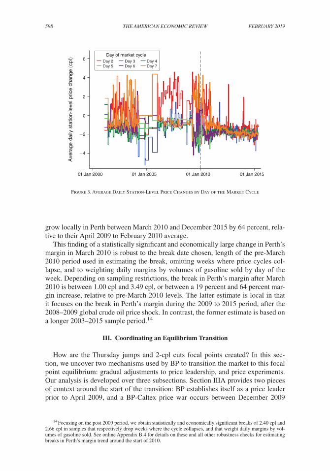
Figure 3 describes inter-temporal dispersion in the magnitude of daily price cuts across stations. Specifically, the figure plots daily average station-level price changes by day of the market cycle. Prior to March 2010, the magnitude of price changes varies substantially across market cycle days and over time.13 However, starting in March 2010, inter-temporal dispersion in daily price changes across sta-tions starts decreasing. At this point, average price changes across days 2 through 7 of the market cycle converge to 2-cpl and remain stable thereafter. This reveals our second focal point of interest: 2-cpl cuts.
B. Margins Grow
Profit margins also start growing in March 2010. We provide evidence of this in panel A of Figure 4, which plots monthly average retail prices for
88 percent for oil majors and supermarkets. Conditional on firm type, stations’ geographic location relative to city center, number of nearby competing stations, and local demographics largely do not predict cycling status.
12 Structural break tests in online Appendix G.2 confirm a structural break exists in April 2009 in the probability that a market price jump occurs on Thursday in a given week. More generally, online Appendix G.2 contains an exhaustive set of structural break tests for breaks in monthly or weekly time series in the timing and magnitude of price jumps and cuts, cycle lengths, and margins at any point in 2009 or 2010. That is, any 2009 or 2010 break discussed in the paper is confirmed using the structural break tests in online Appendix G.2.
13 The time series in Figure 3 thins out in 2005 because of Hurricanes Katrina and Rita, and in 2008–2009 because of a global crude oil price shock. These wholesale cost shocks cause the cycle to collapse. In the years with cycle collapse, there are fewer market cycle days to plot in Figure 3. Online Appendix C provides an in-depth analysis of aggregate shocks and cycle collapses.

597BYRNE AND DE ROOS: LEARNING TO COORDINATEVOL. 109 NO. 2
BP, Caltex, Coles, Woolworths, and Gull, as well as the wholesale TGP. Panel A reveals a widening gap between retail prices and the TGP. Panel B plots correspond-ing monthly average margins and their 12-month moving average. These plots show a break in margin growth in March 2010. Before March 2010, the average daily retail margin is 4.85 cpl (SD = 4.19). After, the average is 10.01 cpl (SD = 4.68), an increase of more than 100 percent.
This margin growth partly reflects a national trend in retail gasoline margins. However, the difference-in-difference estimate of the change in Perth’s retail margin after March 2010 relative to other Australian cities is 3.49 cpl (SE = 0.39). Margins
Panel A. Timing of market price jumps by day of week
Mon
Tue
Wed
Thu
Fri
Sat
Sun
Day
of t
he w
eek
whe
n a
mar
ket p
rice
jum
p oc
curs
01 Jan 2000 01 Jan 2005 01 Jan 2010 01 Jan 2015
Date
MonTueWedThuFriSatSun
Price jump day
Panel B. Average station-level cycle length by �rm and month
0
7
14
21
28
35
Ave
rage
sta
tion-
leve
l cyc
le le
ngth
(day
s)
2000:1 2005:1 2010:1 2015: 1
Month
BP Caltex Woolworths Coles Gull
Figure 2. Timing and Magnitude of Price Jumps and Cycle Length
598 THE AMERICAN ECONOMIC REVIEW FEBRUARY 2019
grow locally in Perth between March 2010 and December 2015 by 64 percent, rela-tive to their April 2009 to February 2010 average.
This finding of a statistically significant and economically large change in Perth’s margin in March 2010 is robust to the break date chosen, length of the pre-March 2010 period used in estimating the break, omitting weeks where price cycles col-lapse, and to weighting daily margins by volumes of gasoline sold by day of the week. Depending on sampling restrictions, the break in Perth’s margin after March 2010 is between 1.00 cpl and 3.49 cpl, or between a 19 percent and 64 percent mar-gin increase, relative to pre-March 2010 levels. The latter estimate is local in that it focuses on the break in Perth’s margin during the 2009 to 2015 period, after the 2008–2009 global crude oil price shock. In contrast, the former estimate is based on a longer 2003–2015 sample period.14
III. Coordinating an Equilibrium Transition
How are the Thursday jumps and 2-cpl cuts focal points created? In this sec-tion, we uncover two mechanisms used by BP to transition the market to this focal point equilibrium: gradual adjustments to price leadership, and price experiments. Our analysis is developed over three subsections. Section IIIA provides two pieces of context around the start of the transition: BP establishes itself as a price leader prior to April 2009, and a BP-Caltex price war occurs between December 2009
14 Focusing on the post 2009 period, we obtain statistically and economically significant breaks of 2.40 cpl and 2.66 cpl in samples that respectively drop weeks where the cycle collapses, and that weight daily margins by vol-umes of gasoline sold. See online Appendix B.4 for details on these and all other robustness checks for estimating breaks in Perth’s margin trend around the start of 2010.
−4
−2
0
2
4
6
Ave
rage
dai
ly s
tatio
n-le
vel p
rice
chan
ge (c
pl)
01 Jan 2000 01 Jan 2005 01 Jan 2010 01 Jan 2015
Day 2 Day 3 Day 4 Day 5 Day 6 Day 7
Day of market cycle
Figure 3. Average Daily Station-Level Price Changes by Day of the Market Cycle

599BYRNE AND DE ROOS: LEARNING TO COORDINATEVOL. 109 NO. 2
and January 2010. In Section IIIB we describe how BP transitions the market to Thursday jumps between April 2009 and August 2012. Section IIIC discusses a separate BP-led transition to 2-cpl cuts that also originates in April 2009, and cul-minates in March 2010.
Panel A. Average station-level prices by �rm and month
80.0
100.0
120.0
140.0
160.0
Ave
rage
sta
tion-
leve
l ret
ail p
rice,
TG
P (c
pl)
2000:1 2005:1 2010:1 2015:1
Month
BP Caltex Woolworths Coles Gull Terminal gate price
Panel B. Average station-level margins by �rm and month
0
5
10
15
Ave
rage
sta
tion-
leve
l ret
ail m
argi
n (c
pl)
2000:1 2005:1 2010:1 2015:1
Month
Figure 4. Monthly Retail Prices, Costs, and Margins
Note: In panel B, average station-level margins by firm and month are in grey scale and their 12-month moving averages are in color.

600 THE AMERICAN ECONOMIC REVIEW FEBRUARY 2019
A. Context for When the Focal Points Emerge
The first notable piece of context is that BP is an established price leader in the market by April 2009. Between 2004 and 2009, BP establishes itself as a price leader in coordinating the market on a price cycle. Over this period, there are three aggregate shocks that disrupt the cycle: (i) Coles’ entry, March 2004–August 2004; (ii)Hurricanes Katrina and Rita, September 2005–December 2005; and (iii) the 2008–2009 global crude oil price shock, June 2008–April 2009.15 BP reinitiates the price cycle after each of these shocks.16 In this way, BP is an established price leader in the market by 2010, with a history of influencing its rivals’ pricing behavior.17
Second, a BP-Caltex price war occurs just prior to the emergence of the focal points in 2010.18 Following the 2008–2009 crude oil price shock, BP reinitiates the cycle in April 2009 by engaging in Wednesday price jumps with its entire station network. All other firms in the market quickly follow BP’s lead and begin coordi-nating on Thursday jumps each week. This pattern of Wednesday jumps by BP, and Thursday jumps by its rivals, remains stable for four months until July 2009. As we will see in Section IIIB, this corresponds to the initiation of Thursday jumps as a pricing focal point, and the start of a three-year equilibrium transition toward a focal pricing equilibrium.
However, starting in August 2009, Caltex defects and starts engaging in Friday jumps, and all other firms quickly follow. Yet BP persists with Wednesday jumps, leaving its stations with 10–15 percent higher prices than its rivals’ prices for two days week-to-week, as per Fuelwatch’s 24-hour rule. BP remains exposed as a two-day price leader for four months between August and November 2009.
In December 2009, BP starts matching its rivals with Friday jumps. In the absence of BP’s Wednesday price jump leadership, the cycle destabilizes between December 2009 and February 2010. It is at this point that BP starts taking steps to cement Thursday jumps and 2-cpl cuts as focal pricing rules.
B. Thursday Jumps
We begin our investigation of focal point formation with Thursday jumps. For our analysis, it is useful to define price jump leadership empirically. Panel A of Figure 5 provides an example that motivates our definition. Panel A tabulates, for each date and firm, the number of stations engaging in station-level price jumps in January 2011. The weekly spikes in the number of stations engaging in price jumps corre-sponds to Thursday price jumps. However, panel A also reveals that a subset of 12 to 16 BP stations engage in price jumps on Wednesdays each week. These stations are price leaders, as their Wednesday jumps help initiate market-wide Thursday jumps.
15 In contrast, price cycles in other Australian cities do not collapse in response to these aggregate shocks, or at any other point between 2001 and 2015. See online Appendix B.2 for an extensive analysis of price cycles in other cities over this period.
16 See online Appendix C for details on aggregate shocks and BP’s leadership role in this period. 17 We can think of two explanations for why BP emerges as a price leader. It has the largest retail station net-
work, and as such can most easily signal price jumps and coordinate market price increases. Moreover, BP operates the only refinery near Perth. If BP is relatively more informed about rivals’ costs and margins, it may be more effective at coordinating price jumps.
18 In online Appendix D, we provide a detailed description of the BP-Caltex price war.

601BYRNE AND DE ROOS: LEARNING TO COORDINATEVOL. 109 NO. 2
In line with Figure 5, we define price jump leadership as follows.
DEFINITION 2: Station i is a price leader on date t if : (i) it engages in a station-level price jump on date t ; (ii) a market cycle begins on date t or t + 1 ; and (iii) less than 2.5 percent of stations engage in station-level price jumps on date t − 1 .
Panel A. Price jumps by �rm: BP Wednesday price jump leadership
0
10
20
30
40
50N
umbe
r of
sta
tion-
leve
l pric
e ju
mps
01 Jan 2011 08 Jan 2011 15 Jan 2011 22 Jan 2011 29 Jan 2011
BP
Caltex
Woolworths
Coles
GullBP priceleadership
Panel B. Price jumps by �rm: No BP Wednesday price jump leadership
0
10
20
30
40
50
Num
ber
of s
tatio
n-le
vel p
rice
jum
ps
01 Jan 2013 08 Jan 2013 15 Jan 2013 22 Jan 2013 29 Jan 2013
Figure 5. BP Price Jump Leadership in 2011 and 2013
602 THE AMERICAN ECONOMIC REVIEW FEBRUARY 2019
This definition encompasses instances where a station engages in a price jump that leads to successful market price jumps the next day, and very few other stations engage in price jumps the previous day.
Returning to Figure 5, we can see two stages in the formation of the Thursday jumps focal point. Whereas panel A shows Wednesday price leadership by BP in January 2011, panel B illustrates cycles in January 2013 where BP Wednesday price leadership does not occur. Instead, all stations coordinate market price jumps with their station networks on Thursdays. We reiterate here, the firms eventually achieve this degree of price coordination despite having to set their prices simultaneously each day.
Creating the Focal Point.—Figure 6 illustrates BP’s transition in price jump lead-ership, and the formation of the Thursday jumps focal point. Panels A and B show the rate at which BP and Caltex converge on Thursday jumps.19 Each panel plots the proportion of station-level price jumps that occur on a given day of the week in a given month. For instance, panel B shows that 20 percent of Caltex stations’ price jumps occur on Thursday in January 2010. By March 2010, this figure jumps to 44 percent. By June 2010, 92 percent of Caltex stations’ price jumps occur on Thursday. For the next five years, between 75 percent and 100 percent of Caltex’s stations’ price jumps occur on Thursdays, month to month.
The dynamics for BP in panel A are different. There is a three-year transition in Thursday jumps (green triangles) and Wednesday jumps (orange circles). Starting in April 2009, nearly 100 percent of BP stations’ price jumps occur on Wednesdays. As per our discussion above, this reflects BP’s re-initiation of the cycle after its col-lapse following the 2008–2009 crude oil price shock. From this point forward, panel A shows a smooth, gradually downward sloping trend in BP stations’ engagement in Wednesday jumps that spans three-years. In August 2012, BP stops engaging in Wednesday jumps altogether.
In contrast, panel A also reveals a smooth upward trend in BP stations’ engage-ment in Thursday jumps. Notice the transition is slower for BP than Caltex. By August 2012, nearly 100 percent of BP station-level price jumps occur on Thursdays, month to month. In sum, panel A of Figure 6 shows BP transitioning from Wednesday jumps to Thursday jumps between April 2009 and August 2012. Through this transition, BP scales back its price jump leadership until it eventually starts coordinating, simultaneously, with its rivals on Thursday jumps. Gradualism in this transition plays an important role: it allows BP to communicate its intentions to its rivals regarding an eventual switch in equilibrium strategy from BP-led weekly price jumps to simultaneous Thursday jumps.
Price Leadership and Signaling.—Figure 7 reveals how BP cements Thursday jumps as a focal point in March 2010, following the BP-Caltex price war. Panels A and B zoom in on the transition to Thursday jumps between September 2009 and September 2010. The panels plot, by brand, the number of stations engaging in Wednesday and Thursday jumps respectively each week in this one-year window.
19 Coles’, Woolworths’, and Gull’s convergences are similar to Caltex’s. See online Appendix G.1.

603BYRNE AND DE ROOS: LEARNING TO COORDINATEVOL. 109 NO. 2
The downward trend in Wednesday price jumps among BP stations from Figure 6 is clear in panel A of Figure 7. Ignoring the eight-week BP-Caltex price war period, for 42 of 44 weeks where the price cycle is stable in panel A, a subset of BP stations lead price jumps on Wednesdays. There are, however, two critical exceptions where BP abandons Wednesday price jump leadership. We label these weeks Gap 1 and Gap 2 in panel A. In these respective weeks, no BP stations engage in Wednesday price jumps.
Panel A. Share of BP station-level price jumps by day of the week and month
BP re-initiatescycle after 2008–09 crude oil price shock
BP stops leadingcycles on Weds.
0
0.2
0.4
0.6
0.8
1
Sha
re o
f sta
tion-
leve
l pric
e ju
mps
day
s in
mon
th
2008:1 2009:1 2010:1 2011:1 2012:1 2013:1 2014:1 2015:1
Month
MonTue
Wed
ThuFriSatSun
Price jumpday
MonTue
Wed
ThuFriSatSun
Price jumpday
Panel B. Share of Caltex station-level price jumps by day of the week and month
0
0.2
0.4
0.6
0.8
1
Sha
re o
f sta
tion-
leve
l pric
e ju
mps
day
s in
mon
th
2008:1 2009:1 2010:1 2011:1 2012:1 2013:1 2014:1 2015:1
Month
Figure 6. BP Price Leadership and the Transition to Thursday Price Jumps

604 THE AMERICAN ECONOMIC REVIEW FEBRUARY 2019
Gap 1 represents an example of BP price leadership that is critical to coordinat-ing the market on the Thursday jumps focal point. In Gap 1, after leading jumps on Wednesdays with the majority of its network for the previous three months, BP has no stations engage in Wednesday price jump leadership. As panel B shows, in Gap 1, 38 of BP’s stations instead engage in Thursday jumps. This one-time break in pricing by BP dramatically affects the market equilibrium. As panel B further shows, prior to Gap 1, BP’s rivals struggle to coordinate on Thursday jumps after
Panel A. Number of station-level price jumps on Wednesdays by �rm and week
Gap 1
Gap 2
BP-Caltexprice war
0
10
20
30
40
50N
umbe
r of
sta
tion-
leve
l pric
e ju
mps
on
Wed
nesd
ay
2009w40 2010w1 2010w13 2010w26 2010w40
Week
BP Caltex Woolworths Coles
BP leadership
BP experiment
Panel B. Number of station-level price jumps on Thursdays by �rm and week
Gap 1Gap 2
0
10
20
30
40
50
Num
ber
of s
tatio
n-le
vel p
rice
jum
ps o
n T
hurs
day
2009w40 2010w1 2010w13 2010w26 2010w40
Week
BP-Caltexprice war
Figure 7. BP Coordinating the Thursday Price Jumps Focal Point

605BYRNE AND DE ROOS: LEARNING TO COORDINATEVOL. 109 NO. 2
the BP-Caltex price war. The week following BP’s Thursday jumps signal in Gap 1, Caltex, Woolworths, and Coles immediately start coordinating on Thursday jumps. At the same time, BP reverts to Wednesday price jump leadership with a subset of stations. From this point onward, Thursday jumps emerges as a stable focal point for coordinating prices.
These dynamics point to BP’s ability, as a price leader, to communicate its inten-tions to its rivals through its prices. Indeed, the sharp shift toward Thursday jumps by BP’s rivals the week immediately after BP signals Thursday jumps in Gap 1 is consistent with BP’s communication directly influencing its rivals’ behavior. The one-time break in BP’s long-run pricing strategy in Gap 1 has sufficient commu-nicative power to transition the market back to having BP Wednesday price jump leadership, and Thursday jumps by BP’s rivals.
Experimentation.—BP appears to engage in a sequence of price experiments as it gradually transitions away from Wednesday price jump leadership. Consider Gap 2 in Figure 7, some ten weeks after Gap 1. For the second time in 2010, BP does not engage in Wednesday price jump leadership, and instead engages in Thursday jumps with 40 stations (panel B).
What is particularly interesting about Gap 2 in panel B of Figure 7, is that both Woolworths and Coles do not have any of their stations engage in Thursday jumps. By contrast, Caltex engages in price jumps, albeit with fewer stations than in the previous ten weeks. This reveals an important piece of information to the mar-ket: Coles and Woolworths do not hold the belief that Thursday jumps are a focal point for coordinating prices among brands. They require BP’s price leadership on Wednesdays to coordinate Thursday jumps.20
For two reasons, we interpret Gap 2 as a BP price experiment. First, it corre-sponds to a one-time break in BP’s long-run pricing strategy of Wednesday price jump leadership. BP’s immediate return to Wednesday price jumps after Gap 2 sug-gests that Gap 2 is not part of a mixed strategy, whereby BP randomizes the day of the week that price jumps occur.
Second, BP runs five additional price experiments like Gap 2 between 2011 and 2013. These are depicted in panels A and B of Figure 8, and are labeled Gap 3 to Gap 7. As a point of reference, we also label Gap 2 in panel A. The plots in Figure 8 are slightly different to those in Figure 7. Figure 8 plots, for each date and firm, the number of stations that successfully lead a market price jump (as per Definition 2), irrespective of whether they lead on a Wednesday, Thursday, or any other day of the week.
The downward-sloping line of green triangles in panel A of Figure 8 corresponds to BP’s transition away from Wednesday price jump leadership between 2009 and 2011. However, Gaps 2 through 4 represent periodic breaks from this trend over this period. For example, panel A depicts a single green triangle with 17 stations in the week before Gap 2. This corresponds to BP alone having 17 stations that lead
20 Woolworths’ and Coles’ stations instead engage in Friday jumps in Gap 2. That is, after BP and Caltex simultaneously engage in Thursday jumps in Gap 2, Woolworths and Coles follow with station-level price jumps on Friday.

606 THE AMERICAN ECONOMIC REVIEW FEBRUARY 2019
with Wednesday price jumps. The rest of the stations in the market follow with a Thursday jump that week.
Recall that in Gap 2, BP stations do not engage in Wednesday jump leadership, and instead engage in Thursday jumps. Coles and Woolworths fail to engage in Thursday jumps in Gap 2, while BP and Caltex, respectively, have 40 and 33 sta-tions simultaneously leading a market price jump on Thursday. Hence, the circled green triangle and blue square in Gap 2 (panel A of Figure 8) highlights a BP exper-iment where BP and Caltex simultaneously lead a Thursday jump. Finally, panel A
Panel A. Number of stations leading market price jumps by �rm: Jul 2010–Jul 2012
Gap2
Gap3
Gap4
Gaps5 6 7
0
10
20
30
40
50
60N
umbe
r of
sta
tions
lead
ing
mar
ket p
rice
jum
ps
01 Jul 2010 01 Janl 2011 01 Jul 2011 01 Jan 2012 01 Jul 2012
Panel B. Number of stations leading market price jumps by �rm: Jan 2012–Jan 2013
Gap5
Gap6
Gap7
Aug 2012: BP Wed. pricejump leadership ends
0
10
20
30
40
50
60
Num
ber
of s
tatio
ns le
adin
g m
arke
t pric
e ju
mps
01 Jan 2012 01 Apr 2012 01 Jul 2012 01 Oct 2012 01 Jan 2013
BPCaltex
WoolworthsColes
BP experiment
Figure 8. BP Experiments with Wednesday Price Jump Leadership and the Thursday Price Jump Focal Point
Note: BP experiment entails weeks without BP Wednesday price jump leadership; firms simultaneously set Thursday price jump.

607BYRNE AND DE ROOS: LEARNING TO COORDINATEVOL. 109 NO. 2
shows that in the week after Gap 2, BP reverts to unilateral leadership, with 17 of its stations engaging in Wednesday jumps.
Gaps 3 and 4 in panel A of Figure 8 are weeks like Gap 2, where BP does not engage in Wednesday price jump leadership. Instead, it coordinates, simultaneously, with its rivals on Thursday jumps. Unlike in Gap 2, Coles and Woolworths coordi-nate on Thursday jumps absent BP Wednesday price leadership in Gaps 3 and 4. From these experiments, Coles and Woolworths appear to have achieved a mutual understanding that Thursday jumps are a focal pricing rule.
Finally, the far-right side of panel A and left half of panel B show that BP rapidly scales back on Wednesday price jump leadership in 2012. BP now generally leads price jumps on Wednesdays with ten or fewer stations. In Gaps 5 to 7, BP runs 3 additional experiments before it permanently stops engaging in Wednesday price jump leadership in August 2012. After more than three years of BP price leadership and experimentation, Thursday jumps are established as a focal point. That is, firms are able to coordinate on the timing of Thursday jumps, absent BP Wednesday price jump leadership.21
Characteristics of Price Jump–Leading BP Stations.—In 2009 and 2010, BP leads price jumps with the same set of stations near the city center for more than eight consecutive weeks at a time.22 Starting in 2011, however, the set of leading BP stations becomes randomly distributed across the city. Moreover, BP starts alter-nating the set of leading stations, and these stations lead for only four consecutive weeks at a time.
In sum, BP starts randomizing which stations lead price jumps across time and space in 2011. However, the price cycle remains stable between 2010 and 2012. These findings potentially reflect the fact that geography plays little role in firms’ monitoring of each other’s current and past actions when a price transparency web-site is available. Consequently, the website could facilitate randomized Wednesday price jump leadership by BP. By randomizing where Wednesday price jumps occur without compromising cycle stability, BP can avoid having particular stations become established as high-priced stations.
C. 2-cpl Cuts
Similar dynamics of price leadership, gradualism, and experimentation exist with the formation of the 2-cpl cuts focal point. These are shown in Figure 9. The figure plots, for each firm and month, the proportion of stations that set an exact 2-cpl daily price cut on cycle days 2, 3, 4, … of a station-level cycle. The figure reveals an initial convergence toward the 2-cpl cut focal point starting in March 2010. Indeed, by April 2010, 68 percent, 55 percent, 68 percent, and 60 percent of BP’s, Caltex’s, Woolworths’, and Coles’ stations respectively are setting 2-cpl daily cuts during the undercutting phase of the cycle. By January 2012, these shares eventually grow to
21 Online Appendix G.3 contains auxiliary results designed to identify alternative explanations for the timing of price experiments. Specifically, we estimate probit models that predict weeks where BP price experiments occur. We find that the experiments are not predicted by payoff-relevant state variables such as wholesale costs, recent success rates in coordinating the size of price jumps across stations, or aggregate macroeconomic shocks.
22 Online Appendix E.2 contains an extensive analysis of the characteristics of price jump-leading BP stations.

608 THE AMERICAN ECONOMIC REVIEW FEBRUARY 2019
89 percent, 67 percent, 94 percent, and 92 percent, respectively. As with Thursday jumps, BP employs gradualism as a price leader in 2010 to communicate its inten-tions to its rivals in transitioning the market to a focal pricing structure that involves 2-cpl cuts.
For the next four years, coordination on the 2-cpl-cut focal point is stable. Even more remarkably, this level of coordination is achieved despite: (i) stations setting prices simultaneously once each day, and (ii) estimates of daily station-level price elasticity of demand on the order of 20 (Clark and Houde 2013), which implies substantial business-stealing incentives to undercut rivals.
Gull’s propensity to conform to the 2-cpl-cut focal point yields an interesting contrast. The figure shows a gradual rise in the propensity of Gull’s stations to set 2-cpl cuts between 2010 and 2013. This difference is consistent with Gull taking longer to learn about the 2-cpl focal point. Alternatively, as an unbranded com-petitor, Gull has proportionately larger business stealing incentives, and thus may initially be more hesitant to coordinate on 2-cpl cuts.
Figure 9 also shows BP temporarily implementing 2-cpl cuts between April and June 2009, before subsequently implementing the focal pricing rule in March 2010. In these three months, between 50 percent and 60 percent of BP stations set pre-cisely 2-cpl cuts, and Caltex and Woolworths both reveal they are willing and able to coordinate on 2-cpl cuts.23 This trialling of 2-cpl cuts by BP, combined with any collective learning about firms’ willingness to coordinate on 2-cpl cuts, facilitates BP price leadership in March 2010 in creating the 2-cpl-cut focal point.24
23 Figure G.2 of online Appendix G.1 shows at weekly frequencies that BP is indeed the first to trial 2-cpl in April 2009, and is followed by Caltex and Woolworths.
24 Figure G.3 in online Appendix G.1 shows that BP price leadership in 2010 and the April-June 2009 trialing of 2-cpl cuts depicted in Figure 9 is unique to 2-cpl cuts.
BP-Caltexprice war
0
0.2
0.4
0.6
0.8
1
Sha
re o
f sta
tions
with
2-c
pl p
rice
cut o
n cy
cle
days
2–7
2009:1 2010:1 2011:1 2012:1 2013:1 2014:1 2015:1
Month
BPCaltexWoolworthsColesGull
Figure 9. BP Price Leadership with 2-Cpl Price Cuts

609BYRNE AND DE ROOS: LEARNING TO COORDINATEVOL. 109 NO. 2
IV. Enhancing Profit Margins
How do the focal points lead to higher margins? In this section, we show that the focal points generate margin growth in two ways: by facilitating coordination on higher price jump margins, and by limiting price undercutting between jumps.
A. Anchoring Margins
Figure 10 highlights an important result for understanding how the focal points enhance margins: they anchor margins to the top of the cycle. To construct the fig-ure, we first compute average retail margins by station-level cycle day and month. We then compute the 12-month moving average of these monthly averages for each cycle day, and plot the moving averages in the figure. The figure shows that after 2010, the difference between margins across consecutive cycle days stabilizes around 2-cpl. Therefore, once the focal points are established, price and margin growth at the top of the cycle directly govern price and margin growth on all other days.25
25 We focus on price and margin levels in Figure 10, and for the remainder of Section IV, because there is min-imal cross-sectional price dispersion day to day. This is particularly the case for the oil majors and supermarkets, which operate 76 percent of the stations in the market after 2010. Online Appendix F.3 provides an in-depth analysis of cross-sectional price dispersion.
0
2
4
6
8
10
12
14
16
18
12-m
onth
mov
ing
aver
age
of m
onth
ly
stat
ion-
leve
l ret
ail m
argi
n (c
pl)
2003
:1
2004
:1
2005
:1
2006
:1
2007
:1
2008
:1
2009
:1
2010
:1
2011
:1
2012
:1
2013
:1
2014
:1
2015
:1
Month
Day 1 Day 6 Day 11 Day 2 Day 7 Day 12 Day 3 Day 8 Day 13 Day 4 Day 9 Day 14 Day 5 Day 10 Day 3
Cycle day
Figure 10. Average Margins by Station-Level Cycle Day and Month
Note: Twelve-month moving averages of the average daily margin by cycle day and month are presented.

610 THE AMERICAN ECONOMIC REVIEW FEBRUARY 2019
B. Coordinating Higher Price Jump Margins
How then do the firms coordinate on higher margins at the top of the cycle? The focal points, combined with BP price jump leadership, create this margin growth. To see this, first consider panel A of Figure 11. The panel plots, for each week and retailer, the difference between the median price among BP stations engaged in leading Wednesday price jumps, and the median price among all other stations on Thursday. The figure shows this difference is zero for 95 percent, 99 percent, 90 percent, and 96 percent of weeks between Gap 1 and August 2012 for BP, Caltex, Woolworths, and Coles, respectively.26 In short, BP stations engaged in Wednesday price jumps signal the Thursday anchor price at the top of the cycle week-to-week.27
BP’s ability to signal Thursday price levels through Wednesday jumps, combined with standardized total price cutting of 12-cpl between Thursday jumps, should imply tightly coordinated prices at the top of the cycle on Thursdays. Panel B of Figure 11, indeed, reveals a remarkable degree of coordination. The figure plots the difference between BP stations’ median price and other firms’ median price on Thursdays. This difference is zero for 95 percent, 89 percent, and 93 percent of weeks between Gap 1 and August 2012 for Caltex, Woolworths, and Coles, respectively.
The focal points, combined with BP price signaling, yield an important result: together, they imply that BP’s choice of Wednesday margins is a key lever through which BP can increase margins at the top of the cycle. Moreover, because the focal points anchor margins to the top of the cycle, by increasing price jump margins on Wednesdays, BP can increase margins on all other days.
Therefore, to complete our analysis of margin growth between March 2010 and August 2012, it remains to show that BP increases price jump margins on Wednesdays over time. Figure 12 shows precisely this: BP gradually increases these margins from 14.2-cpl in March 2010 to 17-cpl in July 2012. This is how BP creates and controls margin growth throughout the market over this period.
C. Price Coordination without Signaling
Returning to panel B of Figure 11, we find another transition in price coordina-tion. There is an immediate and permanent increase in price dispersion on Thursdays starting in August 2012.28 Without BP Wednesday price signaling, firms are less able to coordinate on price jumps. Moreover, BP can no longer directly enhance margins through its choice of Wednesday margins.
Recall, however, that Thursday jumps and 2-cpl cuts remain stable focal points from August 2012 onwards. This implies that firms continue to tightly coordinate on the timing of daily price jumps and cuts, and that margins remain anchored to the
26 The holes in the time series in Figure 11 correspond to Gaps 2 to 7. The instability in panel A at the end of 2011 corresponds to an eight-week period where BP temporarily adjusts Wednesday price signaling. In these weeks, BP sets large 14- to 16-cpl Wednesday jumps that depart from their usual 10- to 12-cpl levels between 2010 and 2012. We show this in online Appendix G.1.
27 Importantly, in signaling prices, leading BP stations “pause” their cycle and have 0-cpl price changes on Thursdays. We show this in online Appendix F.2.
28 Online Appendix F.3 describes in detail the increase in cross-sectional price dispersion in August 2012. Online Appendix G.2 reports results from structural break tests that confirm a break in coordination between BP and its rivals on Thursday margin levels after August 2012.

611BYRNE AND DE ROOS: LEARNING TO COORDINATEVOL. 109 NO. 2
Panel A. Di�erence between median Wed. price among price jump leading BP stations and median Thu. price among non-leading stations
Aug 2012: BP Wed. pricejump leadership ends
−5
−4
−3
−2
-1
0
1
2
3
4
5(M
edia
n W
ed. p
rice
amon
g pr
ice
jum
p le
adin
g B
P s
tatio
ns)
–(m
edia
n T
hu. p
rice
amon
g no
n pr
ice
jum
p le
adin
g st
atio
ns)
2010w1 2010w27 2011w1 2011w27 2012w1 2012w27
Week
Panel B. Di�erence between median Thu. price among all BP stations and median Thu. price among rival stations
Aug 2012: BP Wed. pricejump leadership ends
−5
−4
−3
−2
−1
0
1
2
3
4
5
(M
edia
n T
hu. p
rice
amon
g B
P s
tatio
ns)
–(m
edia
n T
hu. p
rice
amon
g riv
al’s
sta
tions
)
2010w1 2011w1 2012w1 2013w1 2014w1 2015w1Week
(BP Thu. jump price) – (Caltex Thu. jump price)(BP Thu. jump price) – (Woolworths Thu. jump price)(BP Thu. jump price) – (Coles Thu. jump price)
(BP Wed. jump price) – (BP Thu. jump price)(BP Wed. jump price) – (Caltex Thu. jump price)(BP Wed. jump price) – (Woolworths Thu. jump price)(BP Wed. jump price) – (Coles Thu. jump price)
Figure 11. Coordination on Thursday Price Levels

612 THE AMERICAN ECONOMIC REVIEW FEBRUARY 2019
top of the cycle, as shown in Figure 10. Hence, overall margin growth after August 2012 must continue to be driven by larger price jump margins on Thursdays. How then do firms continue to coordinate on higher Thursday margins over time, absent BP price signaling?
We address this question starting with Figure 13, which documents the degree of price coordination by day of the cycle after August 2012. To construct this figure, we first compute the median station-level price across the four major firms’ stations for each date between August 2012 and January 2015. For each date, we then com-pute the difference between each station’s retail price and this median price. We call this difference a station’s pricing error. Panels A and B of Figure 13 plot the distribution of station-level pricing errors by firm on Thursdays (top of the cycle) and Wednesdays (bottom of the cycle).
Panel A shows firms are effective at coordinating on prices on Thursdays absent Wednesday price signaling by BP. Among the major firms’ stations, 91 percent of prices are within 2-cpl of the median on Thursdays between August 2012 and January 2015. These percentages are similar across BP, Caltex, Woolworths, and Coles stations at 91 percent, 94 percent, 89 percent, and 91 percent, respectively.
Contrasting panels A and B of Figure 13, we find that pricing errors for each firm are smaller at the bottom of the cycle. For instance, on day 1 of the cycle, the propor-tion of stations exhibiting 0-cpl pricing errors is 39 percent, 55 percent, 57 percent, and 53 percent for BP, Caltex, Woolworths, and Coles. By day 7 of the cycle, these proportions respectively rise to 58 percent, 69 percent, 90 percent, and 79 percent.29
29 In online Appendix G.4, we show that the proportion of stations exhibiting 0 cpl pricing errors generally falls with each day of the undercutting phase following a price jump.
Gap 1
Aug 2012: BP Wed. pricejump leadership ends
11
12
13
14
15
16
17
18
Med
ian
mar
gin
on W
ed a
mon
g pr
ice
jum
p le
adin
g B
P s
tatio
ns
2010w1 2010w27 2011w1 2011w27 2012w1 2012w27
Week
Median Wed margin among
Price jump leading BP stations12-week moving avg.
Figure 12. Median Margin among Wednesday Price Jump-Leading BP Stations

613BYRNE AND DE ROOS: LEARNING TO COORDINATEVOL. 109 NO. 2
These results point to a self-correcting pricing mechanism whereby firms correct Thursday pricing errors during the undercutting phase of the cycle. Panels A and B of Figure 14 shows how firms correct Thursday mispricing. Panel A plots, by firm, the distribution of daily station-level price changes on Fridays conditional on a sta-tion having a 2-cpl pricing error on Thursday the day before. Panel B presents an analogous plot on daily station-level price changes on Fridays except we condition on stations that had a 1-cpl pricing error on Thursday.
Panel A. Thursdays (cycle day 1)
0
0.1
0.2
0.3
0.4
0.5
0.6
0.7
0.8
0.9
1
Fra
ctio
n of
sta
tion-
leve
l pric
ing
erro
rs
−3 −2 −1 0 1 2 3
Station-level pricing error
−3 −2 −1 0 1 2 3
Station-level pricing error
BP
Caltex
Woolworths
Coles
Panel B. Wednesdays (cycle day 7)
0
0.1
0.2
0.3
0.4
0.5
0.6
0.7
0.8
0.9
1
Fra
ctio
n of
sta
tion-
leve
l pric
ing
erro
rs
Figure 13. Distribution of Station-Level Thursday Pricing Errors Relative to the Median Station-Level Price by Firm between August 2012 and January 2015

614 THE AMERICAN ECONOMIC REVIEW FEBRUARY 2019
The figures show that firms tend to correct overpricing by 2 and 1 cpl above the median on Thursday by cutting prices by 4 and 3 cpl on Friday. That is, if a station overprices on Thursday, their price cut on Friday targets the price level that would have been achieved if the station had matched the median price on Thursday and
Panel A. Station-level Friday price adjustments if 2-cpl above the Thursday median price
0
0.2
0.4
0.6
0.8
1F
ract
ion
of s
tatio
n-le
vel p
rice
chan
ges
−5 −4 −3 −2 −1 0
Friday station-level price change
BP Caltex Woolworths Coles
Panel B. Station-level Friday price adjustments if 1-cpl above the Thursday median price
0
0.2
0.4
0.6
0.8
1
Fra
ctio
n of
sta
tion-
leve
l pric
e ch
ange
s
−5 −4 −3 −2 −1 0
Friday station-level price change
Figure 14. Distribution of Station-Level Friday Price Adjustments Conditional on Mispricing Relative to the Median Station-Level Price on Thursday

615BYRNE AND DE ROOS: LEARNING TO COORDINATEVOL. 109 NO. 2
had cut their price by 2-cpl on Friday (as per the 2-cpl-cut focal pricing rule).30 This pricing error correction process is what enables firms to coordinate on price levels over the cycle, absent BP Wednesday price signaling.31
Our findings are also revealing about how firms gradually enhance margins on Thursdays after August 2012. In particular, a given firm has an incentive to gradu-ally raise its Thursday prices and margins over time as the self-correcting pricing mechanism will lead its rivals to subsequently coordinate on higher prices over the cycle.32 Ultimately, firms’ ability to coordinate on higher margins over time causes Thursday margins to grow from approximately 16-cpl in August 2012 to 19-cpl in January 2015. We illustrate this in Figure 15, which plots median Thursday margins by firm over this period. This implies a 3-cpl margin increase on all days because margins are anchored to the top of the cycle.
30 Online Appendix G.4 presents distributions of daily price changes on Fridays for stations that exhibit 0-cpl, −1-cpl, and −2-cpl pricing errors on Thursdays. Consistent with the results in Figure 14, we find stations tend to have 2-cpl and 1-cpl cuts on Fridays when they exhibit 0-cpl and −1-cpl pricing errors on Thursdays. The results are noisy for −2-cpl pricing errors because these rarely occur, as panel A of Figure 13 shows.
31 Throughout, we have focused on pricing errors relative to the median price across the four major firms’ sta-tions. That is, we have assumed this median price is the anchor price at the top of the cycle. Online Appendix G.4 provides an extensive set of auxiliary results that show firms are more likely to engage in Thursday pricing error corrections on Fridays relative to this median price, rather than correcting pricing errors relative to a particular firm’s median price. That is, we do not find evidence of a “focal firm” for determining the target Thursday margin level between August 2012 and January 2015.
32 Panel A of Figure 13 also reveals a positive bias in pricing errors; more stations raise their price to a level above the median than below. This is also consistent with attempts by firms to coordinate on higher prices over time. Quantitatively, this bias is large: 30 percent of pricing errors are 1- or 2-cpl, whereas only 10 percent of pricing errors are −1- or −2-cpl.
Aug 2012: BP Wed. pricejump leadership ends
14
16
18
20
22
24
26
28
Med
ian
stat
ion-
leve
l pric
e ju
mp
mar
gin
on T
hurs
days
2012w27 2013w1 2013w27 2014w1 2014w27 2015w1
Week
BP Caltex Coles Woolworths Gull
Figure 15. Median Station-Level Margins on Thursdays by Firm between August 2012 and January 2015

616 THE AMERICAN ECONOMIC REVIEW FEBRUARY 2019
Interestingly, we further find minimal change in firms’ margin trends six months before and after August 2012.33 This implies that firms are able to leverage the Thursday jumps and 2-cpl cuts focal points to gradually enhance margins at the same rate with BP price signaling pre-August 2012, and Friday pricing error correc-tions post August 2012.
D. Limiting Price Undercutting
Figure 16 presents our final set of results pertaining to how the focal points facil-itate margin growth. The figure describes margins at the bottom of the cycle by firm and month. To construct the figure, we first restrict the sample to station-dates where Δ p it+1 ≥ 6 cpl for station i on date t .34 Using this sample, we compute monthly average margins by firm. Figure 16 plots these monthly averages in grayscale, and their 12-month moving average in color.
The figure shows that prior to 2010, firms lower prices until they approach mar-ginal costs, at which point price jumps occur. After 2010, with standardized total price cutting of 12-cpl between weekly price jumps, the gap between prices and
33 Online Appendix G.4 contains structural break tests that establish this result. 34 In words, we use station-dates where a station-level price jump occurs on date t + 1 for station i . These dates
correspond to the bottom of each station-level cycle for station i .
–5
0
5
10
12-m
onth
avg
. of s
tatio
n-le
vel r
etai
l mar
gin (c
pl)
2003
:1
2004
:1
2005
:1
2006
:1
2007
:1
2008
:1
2009
:1
2010
:1
2011
:1
2012
:1
2013
:1
2014
:1
2015
:1
Month
BP Caltex Woolworths Coles Gull
Figure 16. Station-Level Margins at the Bottom of the Cycle by Firm and Month
Note: Average station-level margins by firm and month at the bottom of the cycle are in grayscale and their 12-month moving averages are in color.
617BYRNE AND DE ROOS: LEARNING TO COORDINATEVOL. 109 NO. 2
marginal costs is irrelevant for the timing of price jumps. The two focal points, therefore, simultaneously facilitate larger price increases at the top of the cycle, and limit price undercutting at the bottom of the cycle. The softening of price undercut-ting, thus, also contributes to margin growth after 2010.
V. Conclusion
Using a novel dataset, we have studied a coordinated transition by oligopolists to a more profitable equilibrium. Throughout, we have focused on the systematic use of prices rather than explicit communication as a tool for coordination.
Our study informs ongoing debates in law and economics over the role of com-munication in generating collusive outcomes. Economists define an equilibrium as collusive if it delivers greater profits than those available in a static Nash equi-librium, and if such profits are supported by punishments off the equilibrium path. How firms start colluding, and how they decide on a particular collusive strategy, is not part of this standard definition. Acknowledging this, Green, Marshall, and Marx (2015) distinguish between an initiation phase and an implementation phase for collusive agreements. They argue that firms are unlikely to develop a mutual understanding over a collusive strategy absent direct communication in the initi-ation phase.
We contribute to this discussion by demonstrating the communicative power of prices. While we cannot rule out explicit communication between firms, such as phone calls, the heterogeneous and gradual transition of BP’s rivals to a new equilibrium raises concerns of tacit communication by BP through its prices. BP’s price leadership and experiments appear to have facilitated a mutual understanding among rivals of a new, profit-enhancing focal pricing structure.
Given that firms can perfectly monitor fluctuations in rivals’ prices and costs day to day in our setting, it is revealing that BP transitioned the market to a simple pricing structure with Thursday jumps and 2-cpl cuts. This suggests that firms may adopt simple pricing structures, even in the presence of perfect price monitoring, because they are easy to experiment with and communicate to rivals. Moreover, simplicity enhances price transparency and reduces miscommunication. This helps firms identify defections from pricing rules, thereby facilitating adjustments to the pricing structure and enhancing its stability.35
But is transitioning to such a margin-enhancing pricing structure collusive? As Kaplow (2013) thoroughly shows, the legal definition of collusion is highly ambig-uous, which makes such inferences tenuous. As a matter of law, price fixing and other symptoms of collusion are, per se, legal; direct communication that facilitates collusion is, per se, illegal. The law, therefore, targets direct communication as a facilitating practice rather than the practice of price fixing itself.
What then constitutes direct communication? Kaplow (2013) emphasizes a focus on words in antitrust law as the primary medium for direct communication. This motivates the use of evidence obtained from wiretaps or internal industry documents obtained through leniency and immunity programs. In drawing contrast to this focus
35 This standardization of pricing practices by BP is reminiscent of the standardization of rules in the Sugar Institute cartel, documented by Genesove and Mullin (2001).

618 THE AMERICAN ECONOMIC REVIEW FEBRUARY 2019
on words, Kaplow (2013) highlights a convenient quote from Friedman’s landmark paper on repeated games:
[O]ne explanation [for successful coordination] is that [firms’] market moves are interpretable as messages. They converse in a code, as it were. (Friedman 1971, p. 11).
In our study, we interpret various market moves by BP as messages. Price lead-ership and price experiments helped transition the market toward a focal point equi-librium; Wednesday jumps signaled price levels to rivals week to week. In this way, we contribute to ongoing legal debates over the definition of collusion by shedding new light on the potentially important role of prices as a medium for communication in facilitating margin-enhancing price fixing.36
We close by presenting two key policy implications that arise from our study. Our analysis emphasizes the role of firm size asymmetry in facilitating equilibrium coordination: as the dominant firm, BP exploits its size to signal the timing and magnitude of price changes to its rivals, and establish focal points for price coordi-nation. That firm size asymmetry generates coordinated effects contrasts with con-ventional antitrust concerns over mergers that create symmetric firms, as symmetric firms have greater incentives to collude (see, e.g., Ivaldi et al. 2003). A key take-away is that mergers that generate asymmetric firms may also facilitate collusion by enabling price leadership and experimentation.
Our study also highlights the value of detailed data for informing antitrust inves-tigations into conduct. The complete history of daily station-level retail prices over 15 years allowed us to observe retail price distributions effectively in real time. This led to our discovery of a profit-enhancing equilibrium transition, and the price leadership and experiments that facilitated it. It is possible that in emerging data-rich environments in retail markets (e.g., scanner data), antitrust authorities can simi-larly employ high frequency and long panels to guide their investigations. As our analysis has shown, long panels are important because profit-enhancing equilibrium transitions can occur over surprisingly long time horizons, three and a half years in our case. High-frequency data are important because price signals by price leaders on individual dates can be critical in facilitating such transitions. Indeed, BP’s price signaling in March 2010 and its price experiments were critical to the equilibrium transition that we studied.
REFERENCES
Asker, John. 2010. “A Study of the Internal Organization of a Bidding Cartel.” American Economic Review 100 (3): 724–62.
Bain, Joe. 1968. Industrial Organization. 2nd ed. New York: Wiley.Borenstein, Severin, and Andrea Shepard. 1996. “Dynamic Pricing in Retail Gasoline Markets.”
RAND Journal of Economics 27 (3): 429–51.Busse, Meghan R. 2000. “Multimarket Contact and Price Coordination in the Cellular Telephone
Industry.” Journal of Economics and Management Strategy 9 (3): 287–320.Byrne, David P., and Nicolas de Roos. 2018. “Startup Search Costs.” Unpublished.
36 Ezrachi and Stucke (2017) provide a recent example of legal discussion from the OECD pertaining to the definition of collusion. In particular, they discuss emerging legal challenges that big data, machine learning, and “algorithmic collusion” present for anti-trust authorities in defining, identifying, prosecuting, and destabilizing tacit collusion and conscious parallelism.

619BYRNE AND DE ROOS: LEARNING TO COORDINATEVOL. 109 NO. 2
Byrne, David P., and Nicolas de Roos. 2019. “Learning to Coordinate: A Study in Retail Gasoline: Dataset.” American Economic Review. https://doi.org/10.1257/aer.20170116.
Chilet, Jorge Alé. 2018. “Gradually Rebuilding a Relationship: The Emergence of Collusion in Retail Pharmacies in Chile.” Unpublished.
Ciliberto, Federico, and Jonathan W. Williams. 2014. “Does Multimarket Contact Facilitate Tacit Collusion? Inference on Conduct Parameters in the Airline Industry.” RAND Journal of Economics 45 (4): 764–91.
Clark, Robert, and Jean-François Houde. 2013. “Collusion with Asymmetric Retailers: Evidence from a Gasoline Price-Fixing Case.” American Economic Journal: Microeconomics 5 (3): 97–123.
Cramton, Peter, and Jesse A. Schwartz. 2000. “Collusive Bidding: Lessons from the FCC Spectrum Auctions.” Journal of Regulatory Economics 17 (3): 229–52.
Eckert, Andrew. 2013. “Empirical Studies of Gasoline Retailing: A Guide to the Literature.” Journal of Economic Surveys 27 (1): 140–66.
Ezrachi, Ariel, and Maurice E. Stucke. 2017. “Algorithmic Collusion: Problems and Counter-Mea-sures.” Submitted as background material at the Roundtable on Algorithms and Collusion at the OECD Competition Committee.
Friedman, James W. 1971. “A Non-Cooperative Equilibrium for Supergames.” Review of Economic Studies 38 (113): 1–12.
Genesove, David, and Wallace P. Mullin. 2001. “Rules, Communication, and Collusion: Narrative Evidence from the Sugar Institute Case.” American Economic Review 91 (3): 379–98.
Green, Edward J., Robert C. Marshall, and Leslie M. Marx. 2015. “Tacit Collusion in Oligopoly.” In The Oxford Handbook of International Antitrust Economics, Vol. 2, edited by Roger D. Blair and D. Daniel Sokol. Oxford: Oxford University Press.
Harrington, Joseph E., Jr. 2017. “A Theory of Collusion with Partial Mutual Understanding.” Research in Economics 71 (1): 140–58.
Igami, Mitsuru, and Takuo Sugaya. 2018. “Measuring the Incentive to Collude: The Vitamins Cartels, 1990–1999.” Unpublished.
Ivaldi, Marc, Bruno Jullien, Patrick Rey, Paul Seabright, and Jean Tirole. 2003. The Economics of Unilateral Effects: Interim Report for DG Competition, European Commission. Brussels: European Commission.
Kaplow, Louis. 2013. Competition Policy and Price Fixing. Princeton: Princeton University Press. Kawai, Kei, and Jun Nakabayashi. 2018. “Detecting Large-Scale Collusion in Procurement Auctions.”
Unpublished.Knittel, Christopher R., and Victor Stango. 2003. “Price Ceilings as Focal Points for Tacit Collusion:
Evidence from Credit Cards.” American Economic Review 93 (5): 1703–29.Levenstein, Margaret C., and Valerie Y. Suslow. 2006. “What Determines Cartel Success?” Journal of
Economic Literature 44 (1): 43–95.Lewis, Matthew S. 2012. “Price Leadership and Coordination in Retail Gasoline Markets with Price
Cycles.” International Journal of Industrial Organization 30 (4): 342–51.Lewis, Matthew S. 2015. “Odd Prices at Retail Gasoline Stations: Focal Point Pricing and Tacit Collu-
sion.” Journal of Economics and Management Strategy 24 (3): 664–85.Miller, Nathan H., and Matthew C. Weinberg. 2017. “Understanding the Price Effects of the
MillerCoors Joint Venture.” Econometrica 85 (6): 1763–91.National Association of Retail Grocers of Australia. 2010. “Wesfarmers and Woolworths Annual
Reports.” In November 2010 Report—Master Grocers Australia. National Association of Retail Grocers of Australia.
Röller, Lars-Hendrik, and Frode Steen. 2006. “On the Workings of a Cartel: Evidence from the Norwegian Cement Industry.” American Economic Review 96 (1): 321–38.
Schelling, Thomas C. 1960. The Strategy of Conflict. Cambridge, MA: Harvard University Press.Slade, Margaret E. 1992. “Vancouver’s Gasoline-Price Wars: An Empirical Exercise in Uncovering
Supergame Strategies.” Review of Economic Studies 59 (2): 257–76.Stigler, George J. 1964. “A Theory of Oligopoly.” Journal of Political Economy 72 (1): 44–61.Wang, Zhongmin. 2009. “(Mixed) Strategy in Oligopoly Pricing: Evidence from Gasoline Price
Cycles before and under a Timing Regulation.” Journal of Political Economy 117 (6): 987–1030.