Learning Optical Flow

Deqing Sun1, Stefan Roth2, J.P. Lewis3, and Michael J. Black1

1 Department of Computer Science, Brown University, Providence, RI, USA{dqsun,black}@cs.brown.edu

2 Department of Computer Science, TU Darmstadt, Darmstadt, Germanysroth@cs.tu-darmstadt.de

3 Weta Digital Ltd., New Zealandzilla@computer.org

Abstract. Assumptions of brightness constancy and spatial smoothnessunderlie most optical flow estimation methods. In contrast to standardheuristic formulations, we learn a statistical model of both brightnessconstancy error and the spatial properties of optical flow using image se-quences with associated ground truth flow fields. The result is a completeprobabilistic model of optical flow. Specifically, the ground truth enablesus to model how the assumption of brightness constancy is violated innaturalistic sequences, resulting in a probabilistic model of “brightnessinconstancy”. We also generalize previous high-order constancy assump-tions, such as gradient constancy, by modeling the constancy of responsesto various linear filters in a high-order random field framework. Thesefilters are free variables that can be learned from training data. Addition-ally we study the spatial structure of the optical flow and how motionboundaries are related to image intensity boundaries. Spatial smoothnessis modeled using a Steerable Random Field, where spatial derivatives ofthe optical flow are steered by the image brightness structure. Thesemodels provide a statistical motivation for previous methods and enablethe learning of all parameters from training data. All proposed modelsare quantitatively compared on the Middlebury flow dataset.

1 Introduction

We address the problem of learning models of optical flow from training data.Optical flow estimation has a long history and we argue that most methods haveexplored some variation of the same theme. Particularly, most techniques exploittwo constraints: brightness constancy and spatial smoothness. The brightnessconstancy constraint (data term) is derived from the observation that surfacesusually persist over time and hence the intensity value of a small region remainsthe same despite its position change [1]. The spatial smoothness constraint (spa-tial term) comes from the observation that neighboring pixels generally belongto the same surface and so have nearly the same image motion. Despite the longhistory, there have been very few attempts to learn what these terms should be[2]. Recent advances [3] have made sufficiently realistic image sequences withground truth optical flow available to finally make this practical. Here we revisit

D. Forsyth, P. Torr, and A. Zisserman (Eds.): ECCV 2008, Part III, LNCS 5304, pp. 83–97, 2008.c© Springer-Verlag Berlin Heidelberg 2008

84 D. Sun et al.

several classic and recent optical flow methods and show how training data andmachine learning methods can be used to train these models. We then go beyondprevious formulations to define new versions of both the data and spatial terms.

We make two primary contributions. First we exploit image intensity bound-aries to improve the accuracy of optical flow near motion boundaries. The ideais based on that of Nagel and Enkelmann [4], who introduced oriented smooth-ness to prevent blurring of flow boundaries across image boundaries; this can beregarded as an anisotropic diffusion approach. Here we go a step further and usetraining data to analyze and model the statistical relationship between imageand flow boundaries. Specifically we use a Steerable Random Field (SRF) [5]to model the conditional statistical relationship between the flow and the im-age sequence. Typically, the spatial smoothness of optical flow is expressed interms of the image-axis-aligned partial derivatives of the flow field. Instead, weuse the local image edge orientation to define a steered coordinate system forthe flow derivatives and note that the flow derivatives along and across imageboundaries are highly kurtotic. We then model the flow field using a Markovrandom field (MRF) and formulate the steered potentials using Gaussian scalemixtures (GSM) [6]. All parameters of the model are learned from examples thusproviding a rigorous statistical formulation of the idea of Nagel and Enkelmann.

Our second key contribution is to learn a statistical model of the data term.Numerous authors have addressed problems with the common brightness con-stancy assumption. Brox et al. [7], for example, extend brightness constancy tohigh-order constancy, such as gradient and Hessian constancy in order to mini-mize the effects of illumination change. Additionally, Bruhn et al. [8] show thatintegrating constraints within a local neighborhood improves the accuracy ofdense optical flow. We generalize these two ideas and model the data term asa general high-order random field that allows the principled integration of localinformation. In particular, we extend the Field-of-Experts formulation [2] to thespatio-temporal domain to model temporal changes in image features. The dataterm is formulated as the product of a number of experts, where each expert isa non-linear function (GSM) of a linear filter response. One can view previousmethods as taking these filters to be fixed: Gaussians, first derivatives, secondderivatives, etc. Rather than assuming known filters, our framework allows usto learn them from training data.

In summary, by using naturalistic training sequences with ground truth flowwe are able to learn a complete model of optical flow that not only captures thespatial statistics of the flow field but also the statistics of brightness inconstancyand how the flow boundaries relate to the image intensity structure. The modelcombines and generalizes ideas from several previous methods and the result-ing objective function is at once familiar and novel. We present a quantitativeevaluation of the different methods using the Middlebury flow database [3] andfind that the learned models outperform previous models, particularly at motionboundaries. Our analysis uses a single, simple, optimization method throughoutto focus the comparison on the effects of different objective functions. The results

Learning Optical Flow 85

suggest the benefit of learning standard models and open the possibility to learnmore sophisticated ones.

2 Previous Work

Horn and Schunck [9] introduced both the brightness constancy and the spa-tial smoothness constraints for optical flow estimation, however their quadraticformulation assumes Gaussian statistics and is not robust to outliers caused byreflection, occlusion, motion boundaries etc. Black and Anandan [1] introduceda robust estimation framework to deal with such outliers, but did not attemptto model the true statistics of brightness constancy errors and flow derivatives.Fermuller et al. [10] analyzed the effects of noise on the estimation of flow, butdid not attempt to learn flow statistics from examples. Rather than assuming amodel of brightness constancy we acknowledge that brightness can change and,instead, attempt to explicitly model the statistics of brightness inconstancy.

Many authors have extended the brightness constancy assumption, either bymaking it more physically plausible [11,12] or by linear or non-linear pre-filteringof the images [13]. The idea of assuming constancy of first or second imagederivatives to provide some invariance to lighting changes dates back to theearly 1980’s with the Laplacian pyramid [14] and has recently gained renewedpopularity [7]. Following a related idea, Bruhn et al. [8] replaced the pixelwisebrightness constancy model with a spatially smoothed one. They found that aGaussian-weighted spatial integration of brightness constraints results in signif-icant improvements in flow accuracy. If filtering the image is a good idea, thenwe ask what filters should we choose? To address this question, we formulate theproblem as one of learning the filters from training examples.

Most optical flow estimation methods encounter problems at motion bound-aries where the assumption of spatial smoothness is violated. Observing thatflow boundaries often coincide with image boundaries, Nagel and Enkelmann [4]introduced oriented smoothness to prevent blurring of optical flow across imageboundaries. Alvarez et al. [15] modified the Nagel-Enkelmann approach so thatless smoothing is performed close to image boundaries. The amount of smoothingalong and across boundaries has been determined heuristically. Fleet et al. [16]learned a statistical model relating image edge orientation and amplitude to flowboundaries in the context of a patch-based motion discontinuity model. Black[17] proposed an MRF model that coupled edges in the flow field with edgesin the brightness images. This model, however, was hand designed and tuned.We provide a probabilistic framework within which to learn the parameters of amodel like that of Nagel and Enkelmann from examples.

Simoncelli et al. [18] formulated an early probabilistic model of optical flowand modeled the statistics of the deviation of the estimated flow from the trueflow. Black et al. [19] learned parametric models for different classes of flow (e.g.edges and bars). More recently, Roth and Black [2] modeled the spatial structureof optical flow fields using a high-order MRF, called a Field of Experts (FoE), andlearned the parameters from training data. They combined their learned prior

86 D. Sun et al.

model with a standard data term [8] and found that the FoE model improvedthe accuracy of optical flow estimates. While their work provides a learned priormodel of optical flow, it only models the spatial statistics of the optical flow andnot the data term or the relationship between flow and image brightness.

Freeman et al. [20] also learned an MRF model of image motion but theirtraining was restricted to simplified “blob world” scenes; here we use realisticscenes with more complex image and flow structure. Scharstein and Pal [21]learned a full model of stereo, formulated as a conditional random field (CRF),from training images with ground truth disparity. This model also combinesspatial smoothness and brightness constancy in a learned model, but uses simplemodels of brightness constancy and spatially-modulated Potts models for spatialsmoothness; these are likely inappropriate for optical flow.

3 Statistics of Optical Flow

3.1 Spatial Term

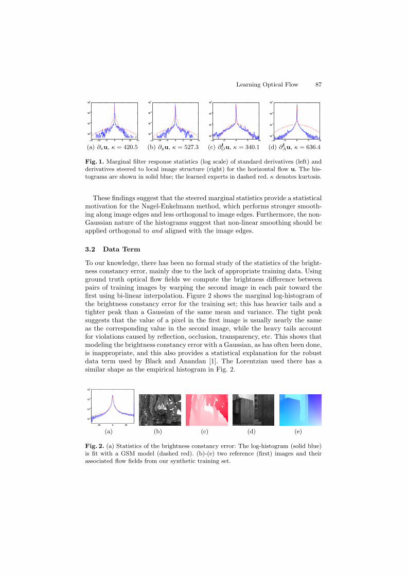
Roth and Black [2] studied the statistics of horizontal and vertical optical flowderivatives and found them to be heavy-tailed, which supports the intuition thatoptical flow fields are typically smooth, but have occasional motion discontinu-ities. Figure 1 (a, b (solid)) shows the marginal log-histograms of the horizontaland vertical derivatives of horizontal flow, computed from a set of 45 groundtruth optical flow fields. These include four from the Middlebury “other” dataset,one from the “Yosemite” sequence, and ten of our own synthetic sequences. Thesesynthetic sequences were generated in the same way as, and are similar to, theother Middlebury synthetic sequences (Urban and Grove); two examples areshown in Fig. 2. To generate additional training data the sequences were alsoflipped horizontally and vertically. The histograms are heavy-tailed with highpeaks, as characterized by their high kurtosis (κ = E[(x − μ)4]/E[(x − μ)2]2).

We go beyond previous work by also studying the steered derivatives of opticalflow where the steering is obtained from the image brightness of the reference(first) frame. To obtain the steered derivatives, we first calculate the local imageorientation in the reference frame using the structure tensor as described in[5]. Let (cos θ(I), sin θ(I))T and (− sin θ(I), cos θ(I))T be the eigenvectors of thestructure tensor in the reference frame I, which are respectively orthogonal toand aligned with the local image orientation. Then the orthogonal and alignedderivative operators ∂I

O and ∂IA of the optical flow are given by

∂IO = cos θ(I) · ∂x + sin θ(I) · ∂y and ∂I

A = − sin θ(I) · ∂x + cos θ(I) · ∂y, (1)

where ∂x and ∂y are the horizontal and vertical derivative operators. We approx-imate these using the 2 × 3 and 3 × 2 filters from [5].

Figure 1 (c, d) shows the marginal log-histograms of the steered derivatives ofthe horizontal flow (the vertical flow statistics are similar and are omitted here).The log-histogram of the derivative orthogonal to the local structure orientationhas much broader tails than the aligned one, which confirms the intuition thatlarge flow changes occur more frequently across the image edges.

Learning Optical Flow 87

−15 −10 −5 0 5 10 15

10−6

10−4

10−2

100

(a) ∂xu, κ = 420.5

−15 −10 −5 0 5 10 15

10−6

10−4

10−2

100

(b) ∂yu, κ = 527.3

−10 −5 0 5 10

10−6

10−4

10−2

100

(c) ∂IOu, κ = 340.1

−10 −5 0 5 10

10−6

10−4

10−2

100

(d) ∂IAu, κ = 636.4

Fig. 1. Marginal filter response statistics (log scale) of standard derivatives (left) andderivatives steered to local image structure (right) for the horizontal flow u. The his-tograms are shown in solid blue; the learned experts in dashed red. κ denotes kurtosis.

These findings suggest that the steered marginal statistics provide a statisticalmotivation for the Nagel-Enkelmann method, which performs stronger smooth-ing along image edges and less orthogonal to image edges. Furthermore, the non-Gaussian nature of the histograms suggest that non-linear smoothing should beapplied orthogonal to and aligned with the image edges.

3.2 Data Term

To our knowledge, there has been no formal study of the statistics of the bright-ness constancy error, mainly due to the lack of appropriate training data. Usingground truth optical flow fields we compute the brightness difference betweenpairs of training images by warping the second image in each pair toward thefirst using bi-linear interpolation. Figure 2 shows the marginal log-histogram ofthe brightness constancy error for the training set; this has heavier tails and atighter peak than a Gaussian of the same mean and variance. The tight peaksuggests that the value of a pixel in the first image is usually nearly the sameas the corresponding value in the second image, while the heavy tails accountfor violations caused by reflection, occlusion, transparency, etc. This shows thatmodeling the brightness constancy error with a Gaussian, as has often been done,is inappropriate, and this also provides a statistical explanation for the robustdata term used by Black and Anandan [1]. The Lorentzian used there has asimilar shape as the empirical histogram in Fig. 2.

−50 0 50

10−6

10−4

10−2

100

(a) (b) (c) (d) (e)

Fig. 2. (a) Statistics of the brightness constancy error: The log-histogram (solid blue)is fit with a GSM model (dashed red). (b)-(e) two reference (first) images and theirassociated flow fields from our synthetic training set.

88 D. Sun et al.

We should also note that the shape of the error histogram will depend on thetype of training images. For example, if the images have significant camera noise,this will lead to brightness changes even in the absence of any other effects. Insuch a case, the error histogram will have a more rounded peak depending onhow much noise is present in the images. Future work should investigate adaptingthe data term to the statistical properties of individual sequences.

4 Modeling Optical Flow

We formulate optical flow estimation as a problem of probabilistic inference anddecompose the posterior probability density of the flow field (u,v) given twosuccessive input images I1 and I2 as

p(u,v|I1, I2; Ω) ∝ p(I2|u,v, I1; ΩD) · p(u,v|I1; ΩS), (2)

where ΩD and ΩS are parameters of the model. Here the first (data) term de-scribes how the second image I2 is generated from the first image I1 and theflow field, while the second (spatial) term encodes our prior knowledge of theflow fields given the first (reference) image. Note that this decomposition of theposterior is slightly different from the typical one, e. g., in [18], in which the spa-tial term takes the form p(u,v; ΩS). Standard approaches assume conditionalindependence between the flow field and the image structure, which is typicallynot made explicit. The advantage our formulation is that the conditional natureof the spatial term allows for more flexible methods of flow regularization.

4.1 Spatial Term

For simplicity we assume that horizontal and vertical flow fields are independent;Roth and Black [2] showed experimentally that this is a reasonable assumption.The spatial model thus becomes

p(u,v|I1; ΩS) = p(u|I1; ΩSu) · p(v|I1; ΩSv). (3)

To obtain our first model of spatial smoothness, we assume that the flow fields areindependent of the reference image. Then the spatial term reduces to a classicaloptical flow prior, which can, for example, be modeled using a pairwise MRF:

pPW(u; ΩPWu) =1

Z(ΩPWu)

∏

(i,j)

φ(ui,j+1−uij; ΩPWu)·φ(ui+1,j−uij; ΩPWu), (4)

where the difference between the flow at neighboring pixels approximates thehorizontal and vertical image derivatives (see e. g., [1]). Z(ΩPWu) here is thepartition function that ensures normalization. Note that although such an MRFmodel is based on products of very local potential functions, it provides a globalprobabilistic model of the flow. Various parametric forms have been used tomodel the potential function φ (or its negative log): Horn and Schunck [9] used

Learning Optical Flow 89

Gaussians, the Lorentzian robust error function was used by Black and Anandan[1], and Bruhn et al. [8] assumed the Charbonnier error function. In this paper,we use the more expressive Gaussian scale mixture (GSM) model [6], i. e.,

φ(x; Ω) =L∑

l=1

ωl · N (x; 0, σ2/sl), (5)

in which Ω = {ωl|l = 1, . . . , L} are the weights of the GSM model, sl are thescales of the mixture components, and σ2 is a global variance parameter. GSMscan model a wide range of distributions ranging from Gaussians to heavy-tailedones. Here, the scales and σ2 are chosen so that the empirical marginals of theflow derivatives can be represented well with such a GSM model and are nottrained along with the mixture weights ωl.

The particular decomposition of the posterior used here (2) allows us to modelthe spatial term for the flow conditioned on the measured image. For example,we can capture the oriented smoothness of the flow fields and generalize theSteerable Random Field model [5] to a steerable model of optical flow, resultingin our second model of spatial smoothness:

pSRF(u|I1; ΩSRFu) ∝∏

(i,j)

φ((∂I1

O u)ij ; ΩSRFu

)· φ

((∂I1

A u)ij ; ΩSRFu

). (6)

The steered derivatives (orthogonal and aligned) are defined as in (1); the su-perscript denotes that steering is determined by the reference frame I1. Thepotential functions are again modeled using GSMs.

4.2 Data Term

Models of the optical flow data term typically embody the brightness constancyassumption, or more specifically model the deviations from brightness constancy.Assuming independence of the brightness error at the pixel sites, we can definea standard data term as

pBC(I2|u,v, I1; ΩBC) ∝∏

(i,j)

φ(I1(i, j) − I2(i + uij , j + vij); ΩBC). (7)

As with the spatial term, various functional forms (Gaussian, robust, etc.) havebeen assumed for the potential φ or its negative log. We again employ a GSMrepresentation for the potential, where the scales and global variance are deter-mined empirically before training the model (mixture weights).

Brox et al. [7] extend the brightness constancy assumption to include high-order constancy assumptions, such as gradient constancy, which may improveaccuracy in the presence of changing scene illumination or shadows. We proposea further generalization of these constancy assumptions and model the constancyof responses to several general linear filters:

pFC(I2|u,v, I1; ΩFC) ∝∏

(i,j)

∏

k

φk{(Jk1 ∗ I1)(i, j)−(Jk2 ∗ I2)(i + uij , j + vij); ΩFC}, (8)

90 D. Sun et al.

where the Jk1 and Jk2 are linear filters. Practically, this equation implies thatthe second image is first filtered with Jk2, after which the filter responses arewarped toward the first filtered image using the flow (u,v) 1. Note that this dataterm is a generalization of the Fields-of-Experts model (FoE), which has beenused to model prior distributions of images [22] and optical flow [2]. Here, wegeneralize it to a spatio-temporal model that describes brightness (in)constancy.

If we choose J11 to be the identity filter and define J12 = J11, this imple-ments brightness constancy. Choosing the Jk1 to be derivative filters and settingJk2 = Jk1 allows us to model gradient constancy. Thus this model generalizesthe approach by Brox et al. [7] 2. If we choose Jk1 to be a Gaussian smoothingfilter and define Jk2 = Jk1, we essentially perform pre-filtering as, for example,suggested by Bruhn et al. [8]. Even if we assume fixed filters using a combinationof the above, our probabilistic formulation still allows learning the parameters ofthe GSM experts from data as outlined below. Consequently, we do not need totune the trade-off weights between the brightness and gradient constancy termsby hand as in [7]. Beyond this, the appeal of using a model related to the FoEis that we do not have to fix the filters ahead of time, but instead we can learnthese filters alongside the potential functions.

4.3 Learning

Our formulation enables us to train the data term and the spatial term sepa-rately, which simplifies learning. Note though, that it is also possible to turnthe model into a conditional random field (CRF) and employ conditional likeli-hood maximization (cf. [23]); we leave this for future work. To train the pairwisespatial term pPW(u; ΩPWu), we can estimate the weights of the GSM model byeither simply fitting the potentials to the empirical marginals using expectationmaximization, or by using a more rigorous learning procedure, such as maximumlikelihood (ML). To find the ML parameter estimate we aim to maximize the log-likelihood LPW(U ; ΩPWu) of the horizontal flow components U = {u(1), . . . ,u(t)}of the training sequences w. r. t. the model parameters ΩPWu (i. e., GSM mixtureweights). Analogously, we maximize the log-likelihood of the vertical componentsV = {v(1), . . . ,v(t)} w. r. t. ΩPWv. Because ML estimation in loopy graphs is gen-erally intractable, we approximate the learning objective and use the contrastivedivergence (CD) algorithm [24] to learn the parameters.

To train the steerable flow model pSRF(u|I1; ΩSRF) we aim to maximize theconditional log-likelihoods LSRF(U|I1; ΩSRFu) and LSRF(V|I1; ΩSRFv) of the

1 It is, in principle, also possible to formulate a similar model that warps the imagefirst and then applies filters to the warped image. We did not pursue this option, asit would require the application of the filters at each iteration of the flow estimationprocedure. Filtering before warping ensures that we only have to filter the imageonce before flow estimation.

2 Formally, there is a minor difference: [7] penalizes changes in the gradient magni-tude, while the proposed model penalizes changes of the flow derivatives. These are,however, equivalent in the case of Gaussian potentials.

Learning Optical Flow 91

training flow fields given the first (reference) images I1 = {I(1)1 , . . . , I(t)

1 } fromthe training image pairs w. r. t. the model parameters ΩSRFu and ΩSRFv.

To train the simple data term pD(I2|u,v, I1; ΩD) modeling brightness con-stancy, we can simply fit the marginals of the brightness violations using ex-pectation maximization. This is possible, because the model assumes indepen-dence of the brightness error at the pixel sites. For the proposed generalized dataterm pFC(I2|u,v, I1; ΩFC) that models filter response constancy, a more complextraining procedure is necessary, since the filter responses are not independent.Ideally, we would maximize the conditional likelihood LFC(I2|U ,V , I1; ΩFC) ofthe training set of the second images I2 = {I(1)

2 , . . . , I(t)2 } given the training flow

fields and the first images. Due to the intractability of ML estimation in thesemodels, we use a conditional version of contrastive divergence (see e. g., [5,23])to learn both the mixture weights of the GSM potentials as well as the filters.

5 Optical Flow Estimation

Given two input images, we estimate the optical flow between them by maxi-mizing the posterior from (2). Equivalently, we minimize its negative log

E(u,v) = ED(u,v) + λES(u,v), (9)

where ED is the negative log (i. e., energy) of the data term, ES is the negativelog of the spatial term (the normalization constant is omitted in either case),and λ is an optional trade-off weight (or regularization parameter).

Optimizing such energies is generally difficult, because of their non-convexityand many local optima. The non-convexity in our approach stems from the factthat the learned potentials are non-convex and from the warping-based dataterm used here and in other competitive methods [7]. To limit the influence ofspurious local optima, we construct a series of energy functions

EC(u,v, α) = αEQ(u,v) + (1 − α)E(u,v), (10)

where EQ is a quadratic, convex, formulation of E that replaces the potentialfunctions of E by a quadratic form and uses a different λ. Note that EQ amountsto a Gaussian MRF formulation. α ∈ [0, 1] is a control parameter that varies theconvexity of the compound objective. As α changes from 1 to 0, the combinedenergy function in (10) changes from the quadratic formulation to the proposednon-convex one (cf. [25]). During the process, the solution at a previous convex-ification stage serves as the starting point for the current stage. In practice, wefind using three stages produces reasonable results.

At each stage, we perform a simple local minimization of the energy. At alocal minimum, it holds that

∇uEC(u,v, α) = 0, and ∇vEC(u,v, α) = 0. (11)

Since the energy induced by the proposed MRF formulation is spatially discrete,it is relatively straightforward to derive the gradient expressions. Setting these

92 D. Sun et al.

to zero and linearizing them, we rearrange the results into a system of linearequations, which can be solved by a standard technique. The main difficulty inderiving the linearized gradient expressions is the linearization of the warpingstep. For this we follow the approach of Brox et al. [7] while using the derivativefilters proposed in [8].

To estimate flow fields with large displacements, we adopt an incrementalmulti-resolution technique (e. g., [1,8]). As is quite standard, the optical flowestimated at a coarser level is used to warp the second image toward the first atthe next finer level and the flow increment is calculated between the first imageand the warped second image. The final result combines all the flow increments.At the first stage where α = 1, we use a 4-level pyramid with a downsamplingfactor of 0.5. At other stages, we only use a 2-level pyramid with a downsamplingfactor of 0.8 to make full use of the solution at the previous convexification stage.

6 Experiments and Results

6.1 Learned Models

The spatial terms of both the pairwise model (PW) and the steerable model(SRF) were trained using contrastive divergence on 20, 000 9 × 9 flow patchesthat were randomly cropped from the training flow fields (see above). To trainthe steerable model, we also supplied the corresponding 20, 000 image patches (ofsize 15× 15 to allow computing the structure tensor) from the reference images.The pairwise model used 5 GSM scales; and the steerable model 4 scales.

The simple brightness constancy data term (BC) was trained using expect-ation-maximization. To train the data term that models the generalized filterresponse constancy (FC), the CD algorithm was run on 20, 000 15 × 15 flowpatches and corresponding 25×25 image patches, which were randomly croppedfrom the training data. 6-scale GSM models were used for both data terms. Weinvestigated two different filter constancy models. The first (FFC) used 3 fixed3 × 3 filters: a small variance Gaussian (σ = 0.4), and horizontal and verticalderivative filters similar to [7]. The other (LFC) used 6 3 × 3 filter pairs thatwere learned automatically. Note that the GSM potentials were learned in eithercase. Figure 3 shows the fixed filters from the FFC model, as well as two of thelearned filters from the LFC model. Interestingly, the learned filters do not looklike ordinary derivative filters nor do they resemble the filters learned in an FoEmodel of natural images [22]. It is also noteworthy that even though the Jk2 arenot enforced to be equal to the Jk1 during learning, they typically exhibit onlysubtle differences as Fig. 3 shows.

Given the non-convex nature of the learning objective, contrastive diver-gence is prone to finding local optima, which means that the learned filtersare likely not optimal. Repeated initializations produced different-looking filters,which however performed similarly to the ones shown here. The fact that these“non-standard” filters perform better (see below) than standard ones suggeststhat more research on better filters for formulating optical flow data terms iswarranted.

Learning Optical Flow 93

(a) (b) (c) (d) (e)

Fig. 3. Three fixed filters from the FFC model: (a) Gaussian, (b) horizontal derivative,and (c) vertical derivative. (d,e) Two of the six learned filter pairs of the LFC modeland the difference between each pair (left: Jk1, middle: Jk2, right: Jk1 − Jk2).

(a) Estimated flow (b) Ground truth (c) Key

Fig. 4. Results of the SRF-LFC model for the “Army” sequence

For the models for which we employed contrastive divergence, we used a hy-brid Monte Carlo sampler with 30 leaps, l = 1 CD step, and a learning rate of0.01 as proposed by [5]. The CD algorithm was run for 2000 to 10000 iterations,depending on the complexity of the model, after which the model parameters didnot change significantly. Figure 1 shows the learned potential functions alongsidethe empirical marginals. We should note that learned potentials and marginalsgenerally differ. This has, for example, been noted by Zhu et al. [26], and isparticularly the case for the SRFs, since the derivative responses are not inde-pendent within a flow field (cf. [5]).

To estimate the flow, we proceeded as described in Section 5 and performed3 iterations of the incremental estimation at each level of the pyramid. Theregularization parameter λ was optimized for each method using a small set oftraining sequences. For this stage we added a small amount of noise to the syn-thetic training sequences, which led to larger λ values and increased robustnessto novel test data.

6.2 Flow Estimation Results

We evaluated all 6 proposed models using the test portion of the Middleburyoptical flow benchmark [3]3. Figure 4 shows the results on one of the sequencesalong with the ground truth flow. Table 1 gives the average angular error (AAE)

3 Note that the Yosemite frames used for testing as part of the benchmark are not thesame as those used for learning.

94 D. Sun et al.

(a) HS [9] (b) BA [1] (c) PW-BC (d) SRF-BC

(e) PW-FFC (f) SRF-FFC (g) PW-LFC (h) SRF-LFC

Fig. 5. Details of the flow results for the “Army” sequence. HS=Horn & Schunck;BA=Black & Anandan; PW=pairwise; SRF=steered model; BC=brightness constancy;FFC=fixed filter response constancy; LFC=learned filter response constancy.

Table 1. Average angular error (AAE) on the Middlebury optical flow benchmark forvarious combinations of the proposed models

Rank Average Army Mequon Schefflera Wooden Grove Urban Yosemite TeddyHS[9] 16.4 8.72 8.01 9.13 14.20 12.40 4.64 8.21 4.01 9.16BA[1] 9.8 7.36 7.17 8.30 13.10 10.60 4.06 6.37 2.79 6.47PW-BC 13.6 8.36 8.01 10.70 14.50 8.93 4.35 7.00 3.91 9.51SRF-BC 10.0 7.49 6.39 10.40 14.00 8.06 4.10 6.19 3.61 7.19PW-FFC 12.6 6.91 4.60 4.63 9.96 9.93 5.15 7.84 3.51 9.66SRF-FFC 9.3 6.26 4.36 5.46 9.63 9.13 4.17 7.11 2.75 7.43PW-LFC 10.9 6.06 4.61 3.92 7.56 7.77 4.76 7.50 3.90 8.43SRF-LFC 8.6 5.81 4.26 4.81 7.87 8.02 4.24 6.57 2.71 8.02

of the models on the test sequences, as well as the results of two standard meth-ods [1,9]. Note that the standard objectives from [1,9] were optimized usingexactly the same optimization strategy as used for the learned models. This en-sures fair comparison and focuses the evaluation on the model rather than theoptimization method. The table also shows the average rank from the Middle-bury flow benchmark, as well as the average AAE across all 8 test sequences.Table 2 shows results of the same experiments, but here the AAE is only mea-sured near motion boundaries. From these results we can see that the steerableflow model (SRF) substantially outperforms a standard pairwise spatial term(PW), particularly also near motion discontinuities. This holds no matter whatdata term the respective spatial term is combined with. This can also be seenvisually in Fig. 5, where the SRF results exhibit the clearest motion boundaries.

Among the different data terms, the filter response constancy models (FFC& LFC) very clearly outperform the classical brightness constancy model (BC),particularly on the sequences with real images (“Army” through “Schefflera”),which are especially difficult for standard techniques, because the classical

Learning Optical Flow 95

Table 2. Average angular error (AAE) in motion boundary regions

Average Army Mequon Schefflera Wooden Grove Urban Yosemite TeddyPW-BC 16.68 14.70 20.70 24.30 26.90 5.40 20.70 5.26 15.50SRF-BC 15.71 13.40 20.30 23.30 26.10 5.07 19.00 4.64 13.90PW-FFC 16.36 12.90 17.30 20.60 27.80 6.43 24.00 5.05 16.80SRF-FFC 15.45 12.10 17.40 20.20 27.00 5.16 22.30 4.24 15.20PW-LFC 15.67 12.80 16.00 18.30 27.30 6.09 22.80 5.40 16.70SRF-LFC 15.09 11.90 16.10 18.50 27.00 5.33 21.50 4.30 16.10

brightness constancy assumption does not appear to be as appropriate as forthe synthetic sequences, for example because of stronger shadows. Moreover,the model with learned filters (LFC) slightly outperforms the model with fixed,standard filters (FFC), particularly in regions with strong brightness changes.This means that learning the filters seems to be fruitful, particularly for challeng-ing, realistic sequences. Further results, including comparisons to other recenttechniques are available at http:// vision.middlebury.edu/ flow/ .

7 Conclusions

Enabled by a database of image sequences with ground truth optical flow fields,we studied the statistics of both optical flow and brightness constancy, andformulated a fully learned probabilistic model for optical flow estimation. Weextended our initial formulation by modeling the steered derivatives of opti-cal flow, and generalized the data term to model the constancy of linear filterresponses. This provided a statistical grounding for, and extension of, variousprevious models of optical flow, and at the same time enabled us to learn allmodel parameters automatically from training data. Quantitative experimentsshowed that both the steered model of flow as well as the generalized data termsubstantially improved performance.

Currently a small number of training sequences are available with groundtruth flow. A general purpose, learned, flow model will require a fully generaltraining set; special purpose models, of course, are also possible. While a smalltraining set may limit the generalization performance of a learned flow model,we believe that training the parameters of the model is preferable to hand tuning(particularly to individual sequences) which has been the dominant approach.

While we have focused on the objective function, the optimization methodmay also play an important role [27] and some models may may admit betteroptimization strategies than others. In addition to improved optimization, futurework may consider modulating the steered flow model by the strength of theimage gradient similar to [4], learning a model that adds spatial integration to theproposed filter-response constancy constraints and thus extends [8], extendingthe learned filter model beyond two frames, automatically adapting the modelto the properties of each sequence, and learning an explicit model of occlusionsand disocclusions.

96 D. Sun et al.

Acknowledgments. This work was supported in part by NSF (IIS-0535075, IIS-0534858) and by a gift from Intel Corp. We thank D. Scharstein, S. Baker,R. Szeliski, and L. Williams for hours of helpful discussion about the evaluationof optical flow.

References

1. Black, M.J., Anandan, P.: The robust estimation of multiple motions: Parametricand piecewise-smooth flow fields. CVIU 63, 75–104 (1996)

2. Roth, S., Black, M.J.: On the spatial statistics of optical flow. IJCV 74, 33–50(2007)

3. Baker, S., Scharstein, D., Lewis, J., Roth, S., Black, M., Szeliski, R.: A databaseand evaluation methodology for optical flow. In: ICCV (2007)

4. Nagel, H.H., Enkelmann, W.: An investigation of smoothness constraints for theestimation of displacement vector fields from image sequences. IEEE TPAMI 8,565–593 (1986)

5. Roth, S., Black, M.J.: Steerable random fields. In: ICCV (2007)

6. Wainwright, M.J., Simoncelli, E.P.: Scale mixtures of Gaussians and the statisticsof natural images. In: NIPS, pp. 855–861 (1999)

7. Brox, T., Bruhn, A., Papenberg, N., Weickert, J.: High accuracy optical flow esti-mation based on a theory for warping. In: Pajdla, T., Matas, J(G.) (eds.) ECCV2004. LNCS, vol. 3024, pp. 25–36. Springer, Heidelberg (2004)

8. Bruhn, A., Weickert, J., Schnorr, C.: Lucas/Kanade meets Horn/Schunck: combin-ing local and global optic flow methods. IJCV 61, 211–231 (2005)

9. Horn, B., Schunck, B.: Determining optical flow. Artificial Intelligence 16, 185–203(1981)

10. Fermuller, C., Shulman, D., Aloimonos, Y.: The statistics of optical flow. CVIU 82,1–32 (2001)

11. Gennert, M.A., Negahdaripour, S.: Relaxing the brightness constancy assumptionin computing optical flow. Technical report, Cambridge, MA, USA (1987)

12. Haussecker, H., Fleet, D.: Computing optical flow with physical models of bright-ness variation. IEEE TPAMI 23, 661–673 (2001)

13. Toth, D., Aach, T., Metzler, V.: Illumination-invariant change detection. In: 4thIEEE Southwest Symposium on Image Analysis and Interpretation, pp. 3–7 (2000)

14. Adelson, E.H., Anderson, C.H., Bergen, J.R., Burt, P.J., Ogden, J.M.: Pyramidmethods in image processing. RCA Engineer 29, 33–41 (1984)

15. Alvarez, L., Deriche, R., Papadopoulo, T., Sanchez, J.: Symmetrical dense opticalflow estimation with occlusions detection. IJCV 75, 371–385 (2007)

16. Fleet, D.J., Black, M.J., Nestares, O.: Bayesian inference of visual motion bound-aries. In: Exploring Artificial Intelligence in the New Millennium, pp. 139–174.Morgan Kaufmann Pub., San Francisco (2002)

17. Black, M.J.: Combining intensity and motion for incremental segmentation andtracking over long image sequences. In: Sandini, G. (ed.) ECCV 1992. LNCS,vol. 588, pp. 485–493. Springer, Heidelberg (1992)

18. Simoncelli, E.P., Adelson, E.H., Heeger, D.J.: Probability distributions of opticalflow. In: CVPR, pp. 310–315 (1991)

19. Black, M.J., Yacoob, Y., Jepson, A.D., Fleet, D.J.: Learning parameterized modelsof image motion. In: CVPR, pp. 561–567 (1997)

Learning Optical Flow 97

20. Freeman, W.T., Pasztor, E.C., Carmichael, O.T.: Learning low-level vision.IJCV 40, 25–47 (2000)

21. Scharstein, D., Pal, C.: Learning conditional random fields for stereo. In: CVPR(2007)

22. Roth, S., Black, M.J.: Fields of experts: A framework for learning image priors. In:CVPR, vol. II, pp. 860–867 (2005)

23. Stewart, L., He, X., Zemel, R.: Learning flexible features for conditional randomfields. IEEE TPAMI 30, 1145–1426 (2008)

24. Hinton, G.E.: Training products of experts by minimizing contrastive divergence.Neural Comput 14, 1771–1800 (2002)

25. Blake, A., Zisserman, A.: Visual Reconstruction. The MIT Press, Cambridge, Mas-sachusetts (1987)

26. Zhu, S., Wu, Y., Mumford, D.: Filters random fields and maximum entropy(FRAME): To a unified theory for texture modeling. IJCV 27, 107–126 (1998)

27. Lempitsky, V., Roth, S., Rother, C.: FusionFlow: Discrete-continuous optimizationfor optical flow estimation. In: CVPR (2008)