learning metapost by doing
TRANSCRIPT

André Heck VOORJAAR 2005 1
Learning METAPOST by Doing
Introduction 1
A Simple Example 2Running METAPOST 2Using the Generated PostScript in a LaTEXDocument 3The Structure of a METAPOST Document 4Numeric Quantities 5If Processing Goes Wrong 6
Basic Graphical Primitives 7Pair 7Path 9Angle and Direction Vector 14Arrow 15Circle, Ellipse, Square, and Rectangle 15Text 16
Style Directives 21Dashing 21Colouring 22Specifying the Pen 23Setting Drawing Options 23
Transformations 24
Advanced Graphics 27Joining Lines 27
Building Cycles 30Clipping 31Dealing with Paths Parametrically 31
Control Structures 34Conditional Operations 34Repetition 37
Macros 39Defining Macros 39Grouping and Local Variables 40Vardef Definitions 41Defining the Argument Syntax 41Precedence Rules of Binary Operators 42Recursion 42Using Macro Packages 44Mathematical functions 45
More Examples 46Electronic Circuits 46Marking Angles and Lines 47Vectorfields 49Riemann Sums 51Iterated Functions 52A Surface Plot 54Miscellaneous 55
Solutions to the exercises 57
Introduction
TEX is the well-known typographic programming language that allows its users toproduce high-quality typesetting especially for mathematical text. METAPOST isthe graphic companion of TEX. It is a graphic programming language developedby John Hobby that allows its user to produce high-quality graphics. It is basedon Donald Knuth’s METAFONT, but with PostScript output and facilities for in-cluding typeset text. This course is only meant as a short, hands-on introductionto METAPOST for newcomers who want to produce rather simple graphics. Themain objective is to get students started with METAPOST on a UNIX platform1. Amore thorough, but also much longer introduction is the Metafun manual of HansHagen [Hag02]. For complete descriptions we refer to the METAPOST Manualand the Introduction to METAPOST of its creator John Hobby [Hob92a, Hob92b].
We have followed a few didactical guidelines in writing the course. Learning isbest done from examples, learning is done from practice. The examples are oftenformatted in two columns, as follows:2
1You can also run METAPOST on a windows platform, e.g., using MikTEX and the WinEdt shell.2On the left is printed the graphic result of the METAPOST code on the right. Here, a square is
drawn.

2 MAPS 32 André Heck
beginfig(1);
draw unitsquare scaled 1cm;
endfig;
The exercises give you the opportunity to practice METAPOST, instead of onlyreading about the program. Compare your answers with the ones in the section‘Solutions to the Exercises’.
A Simple Example
METAPOST is not a WYSIWYG drawing tool like xfig or xpaint. It is a graphicdocument preparation system. First, you write a plain text containing graphicformatting commands into a file by means of your favourite editor. Next, the META-POST program converts this text into a PostScript document that you can previewand print. In this section we shall describe the basics of this process.
Running METAPOST
EXERCISE 1 Do the following steps:
1. Create a text file, say example.mp, that contains the following very simple META-POST document:
beginfig(1);
draw (0,0)--(10,0)--(10,10)--(0,10)--(0,0);
endfig;
end;
For example, you can use the editor XEmacs:
xemacs example.mp
The above UNIX command starts the editor and creates the source fileexample.mp. It is common and useful practice to always give a METAPOST
source file a name with extension .mp. This will make it easier for you to distin-guish the source document from files with other extensions, which METAPOST
will create during the formatting.
2. Generate from this file PostScript code. Here the METAPOST program does thejob:
mpost example
It is not necessary to give the filename extension here. METAPOST now createssome additional files:
example.1 a PostScript file that can be printed and previewed;example.log METAPOST’s log file.
3. Check that the file example.1 contains the following normal Encapsulated Post-Script code:3
3Notice that the bounding box is larger than you might expect, due to the default width of the linedrawing the square.

Learning MetaPost by doing VOORJAAR 2005 3
%!PS
%%BoundingBox: -1 -1 11 11
%%Creator: MetaPost
%%CreationDate: 2003.05.11:2203
%%Pages: 1
%%EndProlog
%%Page: 1 1
0 0.5 dtransform truncate idtransform setlinewidth pop [] 0 setdash
1 setlinecap 1 setlinejoin 10 setmiterlimit
newpath 0 0 moveto
10 0 lineto
10 10 lineto
0 10 lineto
0 10 lineto
0 0 lineto stroke
showpage
%%EOF
4. Preview the PostScript document on your computer screen, e.g., by typing:
gs example.1
You will notice that gs does not use the picture’s bounding box; alternatively, tryggv instead of gs, or:
5. Convert the PostScript document into a printable PDF-document:
epstopdf example.1
It creates the file example.pdf that you can you can view on the computer screenwith the Adobe Acrobat Reader by entering the command:
acroread example.pdf
You can print this file in the usual way. The picture should look like the followingsmall square:
Using the Generated PostScript in a LaTEX Document
EXERCISE 2 Do the following steps:
1. Create a file, say sample.tex, that contains the following lines of LaTEX com-mands that will include the image:
\documentclass{article}
\usepackage{graphicx}
\DeclareGraphicsRule{*}{mps}{*}{}
\begin{document}
\includegraphics{example.1}
\end{document}
Above, we use the extended graphicx package for including the external graphicfile that was prepared by METAPOST. The DeclareGraphicsRule statementcauses all file extensions that are not associated with a well-known graphic formatto be treated as Encapsulated PostScript files.
2. Typeset the LaTEX-file:

4 MAPS 32 André Heck
pdflatex sample
When typesetting is successful, the device independent file sample.pdf is gen-erated.
The Structure of a METAPOST DocumentWe shall use the above examples to explain the basic structure of a METAPOST
document. We start with a closer look at the slightly modified METAPOST code inthe file example.mp of our first example:
beginfig(1); % draw a square
draw (0,0)--(10,0)--(10,10)
--(0,10)--(0,0);
endfig;
end;
This example illustrates the following list of general remarks about regular META-POST files
2 It is recommended to end each METAPOST program in a file with extension mpso that this part of the name can be omitted when invoking METAPOST.
2 Each statement in a METAPOST program is ended by a semicolon. Only in caseswhere the statement has a clear endpoint, e.g., in the end and endfig statement,you may omit superfluous semicolons. We shall not do this in this tutorial. Youcan put two or more statements on one line as long as they are separated bysemicolons. You may also stretch a statement across several lines of code andyou may insert spaces for readability.
2 You can add comments in the document by placing a percentage symbol % infront of the commentary.
2 A METAPOST document normally contains a sequence of beginfig and endfigpairs with an end statement after the last one. The numeric argument to thebeginfig macro determines the name of the output file that will contain thePostScript code generated by the next graphic statements before the correspond-ing endfig command. In the above case, the output of the draw statementbetween beginfig(1) en endfig is written in the file example.1. In general,a METAPOST document consists of one or more instances of
beginfig(figure number);graphic commandsendfig;
followed by end.
2 The draw statement with the points separated by two hyphens (--) draws straightlines that connect the neighbouring points. In the above case for example, thepoint (0,0) is connected by straight lines with the point (10,0) and (0,10).The picture is a square with edges of size 10 units, where a unit is 1
72of an inch.
We shall refer to this default unit as a ‘PostScript point’ or ‘big point’ (bp) todistinguish it from the ‘standard printer’s point’ (pt), which is 1
72.27of an inch.
Other units of measure include in for inches, cm for centimetres, and mm formillimetres. For example,
draw (0,0)--(1cm,0)--(1cm,1cm)--(0,1cm)--(0,0);
generates a square with edges of size 1cm. Here, 1cm is shorthand for 1*cm.You may use 0 instead of 0cm because cm is just a conversion factor and 0cm justmultiplies the conversion factor by zero.

Learning MetaPost by doing VOORJAAR 2005 5
EXERCISE 3 Create a METAPOST file, say exercise3.mp, that generates a circle of diameter2cm using the fullcircle graphic object.
EXERCISE 4 1. Create a METAPOST file, say exercise4.mp, that generates an equilateral tri-angle with edges of size 2cm.
2. Extend the METAPOST document such that it generates in a separate file thePostScript code of an equilateral triangle with edges of size 3cm.
EXERCISE 5 Define your own unit, say 0.5cm, by the statement u=0.5cm; and use this unit uto generate a regular hexagon with edges of size 2 units.
EXERCISE 6 Create the following two pictures:
Numeric QuantitiesNumeric quantities in METAPOST are represented in fixed point arithmetic as in-teger multiples of 1
65536= 2−16 and with absolute value less or equal to 4096 = 212.
Since METAPOST uses fixed point arithmetic, it does not understand exponentialnotation such as 1.23E4. It would interpret this as the real number 1.23, followedby the symbol E, followed by the number 4. Assignment of numeric values canbe done with the usual := operator. Numeric values can be shown via the showcommand.
EXERCISE 7 1. Create a METAPOST file, say exercise7.mp, that contains the following code
numeric p,q,n;
n := 11;
p := 2**n;
q := 2**n+1;
show p,q;
end;
Find out what the result is when you run the above METAPOST program.
2. Replace the value of n in the above METAPOST document by 12 and see whathappens in this case (Hint: press Return to get processing as far as possible).Explain what goes wrong.
3. Insert at the top of the current METAPOST document the following line and seewhat happens now when you process the file.
warningcheck := 0;
The numeric data type is used so often that it is the default type of any non-declaredvariable. This explains why n := 10; is the same as numeric n; n := 10; and

6 MAPS 32 André Heck
why you cannot enter p := (0,0); nor p = (0,0); to define the point, but mustuse pair p; p := (0,0); or pair p; p = (0,0); .
If Processing Goes WrongIf you make a mistake in the source file and METAPOST cannot process your doc-ument without any trouble, the code generation process is interrupted. In the fol-lowing exercise, you will practice the identification and correction of errors.
EXERCISE 8 Deliberately make the following typographical error in the source file example.mp.Change the line
draw (0,0)--(10,0)--(10,10)--(0,10)--(0,0);
into the following two lines
draw (0,0)--(10,0)--(10,10)
draw (10,10)--(0,10)--(0,0);
1. Try to process the document. METAPOST will be unable to do this and theprocessing would be interrupted. The terminal window where you entered thempost command looks like:
(example.mp
! Extra tokens will be flushed.
<to be read again>
addto
draw->addto
.currentpicture.if.picture(EXPR0):also(EXPR0)else:doubl...
<to be read again>
;
l.3 draw (10,10)--(0,10)--(0,0);
?
In a rather obscure way, the METAPOST program notifies the location where itsignals that something goes wrong, viz., at line number 3. However, this doesnot mean that the error is necessarily there.
2. There are several ways to proceed after the interrupt. Enter a question mark andyou see your options:
? ?
Type <return> to proceed, S to scroll future error messages,
R to run without stopping, Q to run quietly,
I to insert something, E to edit your file,
1 or ... or 9 to ignore the next 1 to 9 tokens of input,
H for help, X to quit.
?
3. Press RETURN. METAPOST will continue processing and tries to make the bestof it. Logging continues:
[1] )
1 output file written: example.1
Transcript written on example.log.
4. Verify that only the following path is generated:
newpath 0 0 moveto
10 0 lineto
10 10 lineto stroke
5. Format the METAPOST document again, but this time enter the character e.

Learning MetaPost by doing VOORJAAR 2005 7
Your default editor will be opened and the cursor will be at the location whereMETAPOST spotted the error. Correct the source file4 by adding a semicolon atthe right spot, and give the METAPOST processing another try.
Basic Graphical Primitives
In this section you will learn how to build up a picture from basic graphical prim-itives such as points, lines, and text objects.
PairThe pair data type is represented as a pair of numeric quantities in METAPOST. Onthe one hand, you may think of a pair, say (1,2), as a location in two-dimensionalspace. On the other hand, it represents a vector. From this viewpoint, it is clearthat you can add or subtract two pairs, apply a scalar multiplication to a pair, andcompute the dot product of two pairs.
You can render a point (x,y) as a dot at the specified location with the statement
draw (x,y);
Because the drawing pen has by default a circular shape with a diameter of 1 Post-Script point, a hardly visible point is rendered. You must explicitly scale the drawingpen to a more appropriate size, either locally in the current statement or globallyfor subsequent drawing statements. You can resize the pen for example with a scalefactor 4 by
draw (x,y) withpen pencircle scaled 4; % temporary change of pen
or by
pickup pencircle scaled 4; % new drawing pen is chosen
draw (x,y);
EXERCISE 9 Explain the following result:
beginfig(1)
draw unitsquare scaled 70;
draw (10,20);
draw (10,15) scaled 2;
draw (30,40) withpen pencircle scaled 4;
pickup pencircle scaled 8;
draw (40,50);
draw (50,60);
endfig;
end;
Assignment of pairs is often not done with the usual := operator, but with the equa-tion symbol =. As a matter of fact, METAPOST allows you to use linear equationsto define a pair in a versatile way. A few examples will do for the moment.
2 Using a name that consists of the character z followed by a number, a statementsuch as z0 = (1,2) not only declares that the left-hand side is equal to the right-hand side, but it also implies that the variables x0 and y0 exist and are equal to 1and 2, respectively. Alternatively, you can assign values to the numeric variablex1 and y1 with the result that the pair (x1,y1) is defined and can be referredto by the name z1.
2 A statement like
z1 = -z2 = (3,4);
4If you have not specified another editor in the EDITOR environment variable, then the vi-editor willbe started. You can leave this editor by entering ZZ. In the c-shell you can add in the file .cshrc the linesetenv MPEDIT ’xemacs +%d %s’ so that XEMACS is used.

8 MAPS 32 André Heck
is equivalent to
z1 = (3,4);
z2 = -(3,4);
2 If two pairs, say z1 and z2, are given, you can define the pair, say z3, right inthe middle between these two points by the statement z3 = 1/2[z1,z2].
2 When you have declared a pair, say P, then xpart P and ypart P refer to thefirst and second coordinate of P, respectively. For example,
pair P; P = (10,20);
is the same as
pair P;
xpart P = 10;
ypart P = 20;
EXERCISE 10 Verify that when you use a name that begins with z. followed by a sequence ofalphabetic characters and/or numbers, a statement such as z.P = (1,2) not onlydeclares that the left-hand side is equal to the right-hand side, but it also implies thatthe variables x.P and y.P exist and are equal to 1 and 2, respectively. Alternatively,you can assign values to the numeric variable x.P and y.P, with the result that thepair (x.P,y.P) is defined and can be referred to by the name z.P.
EXERCISE 11 1. Create the following geometrical picture of an acute-angled triangle togetherwith its three medians5:
2. The dotlabel command allows you to mark a point with a dot and to positionsome text around it. For instance, dotlabel.lft("A",(0,0)); generates adot with the label A to the left of the point. Other dotlabel suffixes and theirmeanings are shown in the picture below:
lft rttop
bot
ulft urt
llft lrt
Use the dotlabel command to put labels in the picture in part 1, so that it lookslike
AB
C
A’B’
C’
5The A-median of a triangle ABC is the line from A to the midpoint of the opposite edge BC.

Learning MetaPost by doing VOORJAAR 2005 9
3. Recall that 1/2[z1,z2] denotes the point halfway between the points z1 andz2. Similarly, 1/3[z1,z2] denotes the point on the line connecting the pointsz1 and z2, one-third away from z1. For a numeric variable, which is possiblyunknown yet, c[z1,z2] is c times of the way from z1 to z2. If you do notwant to waste a name for a variable, use the special name whatever to specifya general point on a line connecting two given points:
whatever[z1,z2];
denotes some point on the line connecting the points z1 and z2. Use this fea-ture to define the intersection point of the medians, also known as the centreof gravity, and extend the above picture to the one below. Use the label com-mand, which is similar to the dotlabel command except that it does not draw adot, to position the character G around the centre of gravity. If necessary, assignlabeloffset another value so that the label is further away from the centre ofgravity.
AB
C
A’B’
C’
G
EXERCISE 12 The dir command is a simple way to define a point on the unit circle. For ex-
ample, dir(30); generates the pair (0.86603,0.5)(
= ( 12
√3, 1
2))
. Use the dircommand to generate a regular pentagon.
EXERCISE 13 Use the dir command to draw a line in northwest direction through the point (1, 1)and a line segment through this point that makes an angle of 30 degrees with theline. Your picture should look like
PathOpen and Closed Curves. METAPOST can draw straight lines as well as curvedones. You have already seen that a draw statement with points separated by --draws straight lines connecting one point with another. For example, the result of
draw p0--p1--p2;
after defining three points by
pair p[]; p0 = (0,0); p1 = (2cm,3cm); p2 = (3cm,2cm);
is the following picture.

10 MAPS 32 André Heck
Closing the above path is done either by extending it with --p0 or by connecting thefirst and last point via the cycle command. Thus, the path p0--p1--p2--cycle,when drawn, looks like
The difference between these two methods is that the path extension with the start-ing point only has the optical effect of closing the path. This means that only withthe cycle extension it really becomes a closed path.
EXERCISE 14 Verify that you can only fill the interior of a closed curve with some colour or shadeof gray, using the fill command, when the path is really closed with the cyclecommand. The gray shading is obtained by the directive withcolor c*white,where c is a number between 0 and 1.
Straight and Curved Lines. Compare the pictures from the previous subsectionwith the following ones, which show curves6 through the same points.
u := 1cm;
pair p[];
p0 = (0,0); p1 = (2u,3u); p2 = (3u,2u);
beginfig(1);
draw p0..p1..p2; % draw open curve
for i=0 upto 2:
draw p[i] withpen pencircle scaled 3;
endfor; % draw defining points
endfig;
beginfig(2);
draw p0..p1..p2..cycle; % draw closed curve
for i=0 upto 2:
draw p[i] withpen pencircle scaled 3;
endfor; % draw defining points
endfig;
end;
6the curves through the three points are a circle or a part of the circle

Learning MetaPost by doing VOORJAAR 2005 11
Just use -- where you want straight lines and .. where you want curves.
beginfig(1);
u := 1cm;
pair p[];
p0 = (0,0); p1 = (2u,3u); p2 = (3u,2u);
draw p0--p1..p2..cycle;
for i=0 upto 2:
draw p[i] withpen pencircle scaled 3;
endfor;
endfig;
end;
Construction of Curves. When METAPOST draws a smooth curve through a se-quence of points, each pair of consecutive points is connected by a cubic Béziercurve, which needs, in order to be determined, two intermediate control points inaddition to the end points. The points on the curved segment from points p0 to p1
with post control point c0 and pre control point c1 are determined by the formula
p(t) = (1 − t)3p0 + 3(1 − t)2tc0 + 3(1 − t)t2c1 + t3p1 ,
where t ∈ [0, 1]. METAPOST automatically calculates the control points such thatthe segments have the same direction at the interior knots. In the figure below, theadditional control points are drawn as gray dots and connected to their parent pointwith gray line segments. The curve moves from the starting point in the directionof the post control point, but possibly bends after a while in another direction. Thefurther away the post control point is, the longer the curve keeps this direction.Similarly, the curve arrives at a point coming from the direction of the pre controlpoint. The further away the pre control point is, the earlier the curve gets thisdirection. It is as if the control points pull their parent point in a certain directionand the further away a control point is, the stronger it pulls. By default in META-POST, the incoming and outgoing direction at a point on the curve are the sameso that the curve is smooth.
u := 1.25cm;
color gray; gray := 0.6white;
pair p[];
p0 = (0,0); p1 = (2u,3u); p2 = (3u,2u);
def drawpoint(expr z, c) = draw z
withpen pencircle scaled 3 withcolor c;
enddef;
beginfig(1);
path q; q := p0..p1..p2;
for i=0 upto length(q):
drawpoint(point i of q, black);
p3 := precontrol i of q;
p4 := postcontrol i of q;
draw p3--p4 withcolor gray;
drawpoint(p3, gray);
drawpoint(p4, gray);
endfor;
draw q;
endfig;

12 MAPS 32 André Heck
beginfig(2);
path q; q := p0..p1..p2..cycle;
for i=0 upto length(q):
drawpoint(point i of q, black);
p3 := precontrol i of q;
p4 := postcontrol i of q;
draw p3--p4 withcolor gray;
drawpoint(p3, gray);
drawpoint(p4, gray);
endfor;
draw q;
endfig;
end;
Do not worry when you do not understand all details of the above METAPOST
program. It contains features and programming constructs that will be dealt withlater in the tutorial.
There are various ways of controlling curves:
2 Vary the angles at the start and end of the curve with one of the keywords up,down, left, and right, or with the dir command.
2 Specify the requested control points manually.
2 Vary the inflection of the curve with tension and curl. tension influences thecurvature, whereas curl influences the approach of the starting and end points.
pair p[]; p0:=(0,0); p1:=(1cm,1cm);
def drawsquare = draw unitsquare
scaled 1cm withcolor 0.7white;
enddef;
beginfig(1);
drawsquare; drawarrow p0..p1;
endfig;
beginfig(2);
drawsquare; drawarrow p0{right}..p1;
endfig;
beginfig(3);
drawsquare; drawarrow p0{up}..p1;
endfig;
beginfig(4);
drawsquare; drawarrow p0{left}..p1;
endfig;

Learning MetaPost by doing VOORJAAR 2005 13
beginfig(5);
drawsquare; drawarrow p0{down}..p1;
endfig;
beginfig(6);
drawsquare; drawarrow p0{dir(-45)}..p1;
endfig;
beginfig(7);
drawsquare; drawarrow p0..
controls (0,1cm) and (1cm,0) ..p1;
endfig;
beginfig(8);
drawsquare; drawarrow p0{curl 80}..
(0,-1cm)..{curl 8}p1;
endfig;
beginfig(9);
drawsquare; drawarrow p0..tension(2)
..(0,1cm)..p1;
endfig;
end;
The METAPOST operators --, ---, and ... have been defined in terms of curland tension directives as follows:
def -- = {curl 1}..{curl 1} enddef;
def --- = .. tension infinity .. enddef;
def ... = .. tension atleast 1 .. enddef;
The meaning of ... is “choose an inflection-free path between the points unless theendpoint directions make this impossible”. The meaning of --- is “get a smoothconnection between a straight line and the rest of the curve”.
pair p[]; p0:=(0,0); p1:=(1cm,1cm);
def drawsquare = draw unitsquare scaled 1cm
withcolor 0.7white;
enddef;
beginfig(1);
drawsquare; drawarrow p0---(1.5cm,0)..p1;
endfig;
beginfig(2);
drawsquare; drawarrow p0...(1.5cm,0)..p1;
endfig;
end;
The above examples were also meant to give you the impression that you can drawin METAPOST almost any curve you wish.
EXERCISE 15 Draw an angle of 40 degrees that looks like

14 MAPS 32 André Heck
EXERCISE 16 Draw a graph that looks like
EXERCISE 17 Draw the Yin-Yang symbol7 that looks like
Angle and Direction VectorIn a previous exercise you have already seen that the dir command generates apair that is a point on the unit circle at a given angle with the horizontal axis. Theinverse of dir is angle, which takes a pair, interprets it as a vector, and computesthe two-argument arctangent, i.e., it gives the angle corresponding with the vector.In the example below we use it to draw a bisector of a triangle.
AB
C
C’
pair A, B, C, C’;
u := 1cm; A=(0,0); B=(5u,0); C=(2u,3u);
C’ = whatever[A,B] = C + whatever*dir(
1/2*angle(A-C)+1/2*angle(B-C));
beginfig(1)
draw A--B--C--cycle; draw C--C’;
dotlabel.lft("A",A); dotlabel.urt("B",B);
dotlabel.top("C",C); dotlabel.bot("C’",C’);
endfig;
end;
EXERCISE 18 Change the above picture to the following geometrical diagram, which illustratesbetter that a bisector is actually drawn for the acute-angled triangle.
AB
C
C’
EXERCISE 19 Draw a picture that shows all the bisectors of a acute-angled triangle. Your pictureshould look like
7See www.chinesefortunecalendar.com/YinYang.htm for details about the symbol.

Learning MetaPost by doing VOORJAAR 2005 15
A
B
C
A’B’
C’
I
In this way, it illustrates that the bisectors of a triangle go through one point, theso-called incenter, which is the centre of the inner circle of the triangle.
ArrowThe drawarrow command draws the given path with an arrowhead at the end. Fordouble-headed arrows, simply use the drawdblarrow command. A few examples:
beginfig(1);
drawarrow (0,0)--(60,0);
drawarrow reverse((0,-20)--(60,-20))
withpen pencircle scaled 2;
drawdblarrow (0,-40)--(60,-40);
drawarrow (0,-65){dir(30)}..
{dir(-30)}(60,-65);
drawarrow (0,-90){dir(-30)}..{up}(60,-90)..
{dir(-150)}cycle;
endfig;
end;
If you want arrowheads of different size, you can change the arrowhead lengththrough the variable ahlength (4bp by default) and you can control the angle atthe tip of the arrowhead with the variable ahangle (45 degrees by default). You canalso completely change the definition of the arrowhead procedure. In the examplebelow, we draw a curve with an arrow symbol along the path. As a matter of fact,the path is drawn in separate pieces that are joined together with the & operator.
beginfig(1);
save arrowhead;
vardef arrowhead(expr p) =
save A,u,a,b; pair A,u; path a,b;
A := point length(p)/2 of p;
u := unitvector(direction length(p)/2 of p);
a := A{-u}..(A - ahlength*u rotated 30);
b := A{-u}..(A - ahlength*u rotated -30);
(a & reverse(a) & b & reverse(b))--cycle
enddef;
u:=2cm; ahlength:=0.3cm;
drawarrow (0,0)..(u,u)..(-u,u);
endfig; end;
Circle, Ellipse, Square, and RectangleYou have already seen that you can draw a circle through three points z0, z1, andz2, that do not lie on a straight line with the statement draw z0..z1..z2..cycle;.But METAPOST also provides predefined paths to build circles and circular disksor parts of them. Similarly, you can draw a rectangle once the four corner points, sayz0, z1, z2, and z3, are known with the statement draw z0--z1--z2--z3--cycle;.The path (0,0)--(1,0)--(1,1)--(0,1)--cycle is in METAPOST predefined asunitsquare.

16 MAPS 32 André Heck
Path Definition
fullcircle circle with diameter 1 and centre (0, 0).halfcircle upper half of fullcirclequartercircle first quadrant of fullcircleunitsquare (0,0)--(1,0)--(1,1)--cyle
You can construct from these basic paths any circle, ellipse, square, or rectangleby rotating (rotated operator), by scaling (operators scaled, xscaled, andyscaled), and/or by translating the graphic object (shifted operator). Keep inmind that the ordering of operators has a strong influence on the final shape. Butpictures say more than words. The diagram
is drawn with the following METAPOST code.
beginfig(1);
u := 24; % 24 = 24bp = 1/3 inch
for i=-1 upto 9: draw (i*u,4u)--(i*u,-3u) withcolor 0.7white; endfor;
for i=-3 upto 4: draw (-u,i*u)--(9u,i*u) withcolor 0.7white; endfor;
dotlabel("",origin); % the grid with reference point (0,0) has been drawn
draw fullcircle scaled u;
draw halfcircle scaled u shifted (2u,0);
draw quartercircle scaled u shifted (4u,0);
draw fullcircle xscaled 2u yscaled u shifted (6u,0);
draw fullcircle xscaled 2u yscaled u rotated -45 shifted (8u,0);
fill fullcircle scaled u shifted (0,-2u);
fill halfcircle--cycle scaled u shifted (2u,-2u);
path quarterdisk; quarterdisk := quartercircle--origin--cycle;
fill quarterdisk scaled u shifted (4u,-2u);
fill quarterdisk scaled u rotated -45 shifted (6u,-2u);
fill quarterdisk scaled u shifted (6u,-2u) rotated 45;
fill quarterdisk rotated -90 scaled 2u shifted (8u,3u);
fill unitsquare scaled u shifted (0,2u);
fill unitsquare xscaled u yscaled 3/2u shifted (2u,2u);
endfig;
end;
TextYou have already seen how the dotlabel command can be used to draw a dot anda label in the neighbourhood of the dot. If you do not want the dot, simply use the

Learning MetaPost by doing VOORJAAR 2005 17
label command:
label.suffix(string expression, pair);
It uses the same suffixes as the dotlabel command to position the label relativeto the given pair. No suffix means that the label is printed with its centre at thespecified location Available directives for the specification of the label relative tothe given pair are (see also page 8):
top : top ulft : upper leftlft : left urt : upper rightrt : right lrt : lower right
bot : bot llft : lower left
The distance from the pair to the label is set by the numeric variable labeloffset.The commands label and dotlabel both use a string expression for the label
text and typeset it in the default font, which is likely to be "cmr10" and which canchanged through the variables defaultfont and defaultscale. For example,
defaultfont := "ptmr";
defaultscale := 12pt/fontsize(defaultfont);
makes labels come out as Adobe Times-Roman at about 12 points.
Until now the string expression in a text command has only been a string delimitedby double quotes (optionally joined to another string via the concatenation operator&). But you can also bracket the text with btex and etex (do not put it in quotesthis time) and pass it to TEX for typesetting. This allows you to use METAPOST
in combination with TEX for building complex labels. Let us begin with a simpleexample:
√3
12
beginfig(1);
z0 = (0,0); z1 = (sqrt(3)*cm,0);
z2 = (sqrt(3)*cm,1cm);
draw z0--z1--z2--cycle;
label.bot(btex $\sqrt{3}$ etex, 1/2[z0,z1]);
label.rt(btex 1 etex, 1/2[z1,z2]);
label.top(btex 2 etex, 1/2[z0,z2]);
endfig;
end;
Whenever the METAPOST program encounters btex typesetting commands etex,it suspends the processing of the input in order to allow TEX to typeset the com-mands and the dvitomp preprocessor to translate the typeset material into a pictureexpression that can be used in a label or dotlabel statement. The generated lowlevel METAPOST code is placed in a file with extension .mpx. Hereafter META-POST resumes its work.
We speak about a picture expression that is created by typesetting commandsbecause it is a graphic object to which you can apply transformation. This is il-lustrated by the following example, in which we use diagonal curly brackets andtext.

18 MAPS 32 André Heck
{ }{
√3
12
beginfig(1);
z0 = (0,0); z1 = (sqrt(3)*cm,0);
z2 = (sqrt(3)*cm,1cm);
draw z0--z1--z2--cycle;
label.bot(btex $\lbrace$ etex rotated 90
xscaled 5 yscaled 1.4, 1/2[z0,z1]);
label.rt((btex $\rbrace$ etex) xscaled 1.3
yscaled 3, 1/2[z1,z2]);
label(btex $\lbrace$ etex xscaled 1.5 yscaled 5.7
rotated -60, 1/2[z0,z2] + dir(120)*2mm);
labeloffset:=3.5mm;
label.bot(btex $\sqrt{3}$ etex, 1/2[z0,z1]);
label.rt(btex 1 etex, 1/2[z1,z2]);
label(btex 2 etex, 1/2[z0,z2]+dir(120)*5mm);
endfig;
end;
Until now we have only used plain TEX commands. But what if you want torun another TEX-version? The following example shows how you can use averbatimtex.....etex block to specify that LaTEX is used and which style and/orpackages are chosen.
√3
1
2
1
verbatimtex
%&latex
\documentclass{article}
\begin{document}
etex
beginfig(1);
z0 = (0,0); z1 = (sqrt(3)*cm,0);
z2 = (sqrt(3)*cm,1cm);
draw z0--z1--z2--cycle;
label.bot(btex $\sqrt{3}$ etex, 1/2[z0,z1]);
label.rt(btex $\frac{1}{2}$ etex, 1/2[z1,z2]);
label.top(btex 1 etex, 1/2[z0,z2]);
endfig;
end;
One last remark about using LaTEX: Between btex and etex, you can-not use displayed math mode such as $$\frac{x}{x+1}$$. You must use$\displaystyle \frac{x}{x+1}$ instead.
Let us use what we have learned so far in this chapter in a more practical ex-
ample: drawing the graph of the function x 7→ ex
1 + xfrom 0 to 5 with the vertical
axis in a logarithmic scale. The picture is generated by the following METAPOST
code:
verbatimtex
%&latex
\documentclass{article}
\begin{document}
etex
% some function definitions
vardef exp(expr x) = (mexp(256)**x) enddef;
vardef ln(expr x) = (mlog(x)/256) enddef;
vardef log(expr x) = (ln(x)/ln(10)) enddef;
vardef f(expr x) = (exp(x)/(1+x)) enddef;
ux := 1cm; uy := 4cm;

Learning MetaPost by doing VOORJAAR 2005 19
0 1 2 3 4 5 61
10
100
5
50 graph of x 7→ ex
1 + x
linear scale
logari
thm
icsc
ale
beginfig(1)
numeric xmin, xmax, ymin, ymax;
xmin := 0; xmax := 6;
ymin := 0; ymax := 2;
% draw axes
draw (xmin,0)*ux -- (xmax+1/2,0)*ux;
draw (0,ymin)*uy -- (0,ymax+1/10)*uy;
% draw tickmarks and labels on horizontal axis
for i=0 upto xmax:
draw (i,-0.05)*ux--(i,0.05)*ux;
label.bot(decimal(i),(i,0)*ux);
endfor;
% draw tickmarks and labels on vertical axis
for i=2 upto 10:
draw (-0.01,log(i))*uy--(0.01,log(i))*uy;
draw (-0.01,log(10*i))*uy--(0.01,log(10*i))*uy;
endfor;
for i=0 upto 2: label.lft(decimal(10**i), (0,i)*uy); endfor;
for i=0 upto 1: label.lft(decimal(5*(10**i)),
(0,log(5*(10**i)))*uy); endfor;
% compute and draw the graph of the function
xinc := 0.1;
path pts_f;
pts_f := (xmin*ux,log(f(xmin))*uy)
for x=xmin+xinc step xinc until xmax:
.. (x*ux,log(f(x))*uy)
endfor;
draw pts_f withpen pencircle scaled 2;
% draw title
label(btex graph of $\displaystyle x\mapsto\frac{eˆx}{1+x}$
etex, (2ux,1.7uy));
% draw axis explanation
labeloffset := 0.5cm;
label.bot(btex linear scale etex, (3,0)*ux);
label.lft(btex logarithmic scale etex rotated(90),
(0,1)*uy);
endfig;
end;
The above code needs some explanation.First of all, METAPOST does not know about the exponential or logarithmic
function. But you can easily define these functions with the help of the built-infunctions mexp(x) = exp(x/256) and mlog(x) = 256 ln x . Note that we have re-served the name log for the logarithm with base 10 in the above program.
As you will see later in this tutorial, METAPOST has several repetition controlstructures. Here we apply the for loop to draw tick marks and labels on the axesand to compute the path of the graph. The basic form is:
for counter = start step stepsize until finish :loop text
endfor;
Instead of step 1 until, you may use the keyword upto. downto is another wordfor step -1 until.
In the following code snippet
for i=0 upto xmax:
draw (i,-0.05)*ux--(i,0.05)*ux;
label.bot(decimal(i),(i,0)*ux);
endfor;
the input lines are two statements: one to draw tick marks and the other to put alabel. We use the decimal command to convert the numeric variable i into a string

20 MAPS 32 André Heck
so that we can use it in the label statement. The following code snippet
pts_f := (xmin*ux,log(f(xmin))*uy)
for x=xmin+xinc step xinc until xmax:
.. (x*ux,log(f(x))*uy)
endfor;
shows that you can also use the for loop to build up a single statement. The inputlines within the for loop are pieces of a path definition. This mode of creating astatement may look strange at first sight, but it is an opportunity given by the factthat METAPOST consists more or less of two parts: a preprocessor and a PostScriptgenerator. The preprocessor only reads from the input stream and prepares inputfor the PostScript generator.
EXERCISE 20 Draw the graph of the function x 7→ √x on the interval (0, 2). Your picture should
look like
0 1 2 3 40
1
2
x
yy =
√x
Your METAPOST code should be such that only a minimal change in the code isrequired to draw the graph on a different domain, say [0, 3].
EXERCISE 21 Draw the following picture in METAPOST. The dashed lines can be drawn byadding dashed evenly at the end of the draw statement.
0 a
ib
C
a + ib = z{ |z|
φ
EXERCISE 22 The annual beer consumption in the Netherlands in the period 1980–2000 is listedbelow.
year 1980 1985 1990 1995 2000
litre 86 85 91 86 83
Draw the following graph in METAPOST.

Learning MetaPost by doing VOORJAAR 2005 21
19801985199019952000
82
84
86
88
90
92
year
bee
rco
nsu
mption
(liter
)
Style Directives
In this section we explain how you can alter the appearance of graphics primitives,e.g., allowing certain lines to be thicker and others to be dashed, using differentcolours, and changing the type of the drawing pen.
DashingExamples show you best how the specify a dash pattern when drawing a line orcurve.
beginfig(1);
path p; p := (0,0)--(102,0);
def drawit (suffix p)(expr pattern) =
draw p dashed pattern;
p := p shifted (0,-13);
enddef;
drawit(p, withdots);
drawit(p, withdots scaled 2);
drawit(p, evenly);
drawit(p, evenly scaled 2);
drawit(p, evenly scaled 4);
drawit(p, evenly scaled 6);
p := (0,-150)--(102,-150);
def shiftit (suffix p)(expr s) =
draw p dashed evenly scaled 4 shifted s;
dotlabel("",point 0 of p);
dotlabel("",point 1 of p);
p := p shifted (0,-13);
enddef;
shiftit(p, (0,0));
shiftit(p, (4bp,0));
shiftit(p, (8bp,0));
shiftit(p, (12bp,0));
shiftit(p, (16bp,0));
shiftit(p, (20bp,0));
picture dd; dd :=
dashpattern(on 6bp off 2bp on 2bp off 2bp);
draw (0,-283)--(102,-283) dashed dd;
draw (0,-296)--(102,-296) dashed dd scaled 2;
endfig;
end;
In general, the syntax for dashing is
draw path dashed dash pattern;
22 MAPS 32 André Heck
You can define a dash pattern with the dashpattern function whose argument isa sequence of on/off distances. Predefined patterns are:
evenly = dashpattern(on 3 off 3); % equal length dashes
withdots = dashpattern(off 2.5 on 0 off 2.5); % dotted lines
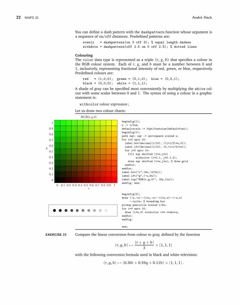
ColouringThe color data type is represented as a triple (r, g, b) that specifies a colour inthe RGB colour system. Each of r, g, and b must be a number between 0 and1, inclusively, representing fractional intensity of red, green, or blue, respectively.Predefined colours are:
red = (1,0,0); green = (0,1,0); blue = (0,0,1);
black = (0,0,0); white = (1,1,1);
A shade of gray can be specified most conveniently by multiplying the white col-our with some scalar between 0 and 1. The syntax of using a colour in a graphicstatement is:
withcolor colour expression;
Let us draw two colour charts:
0
0
0.1
0.1
0.2
0.2
0.3
0.3
0.4
0.4
0.5
0.5
0.6
0.6
0.7
0.7
0.8
0.8
0.9
0.9
1
1
r
g
RGB(r,g,0)
beginfig(1);
u := 1/2cm;
defaultscale := 10pt/fontsize(defaultfont);
beginfig(1);
path sqr; sqr := unitsquare scaled u;
for i=0 upto 10:
label.bot(decimal(i/10), ((i+1/2)*u,0));
label.lft(decimal(i/10), (0,(i+1/2)*u));
for j=0 upto 10:
fill sqr shifted (i*u,j*u)
withcolor (i*0.1, j*0.1,0);
draw sqr shifted (i*u,j*u); % draw grid
endfor;
endfor;
label.bot("r",(6u,-2/3u));
label.lft("g",(-u,6u));
label.top("RGB(r,g,0)", (6u,11u));
endfig; end;
beginfig(2);
draw (-u,-u)--(11u,-u)--(11u,u)--(-u,u)
--cycle; % bounding box
pickup pencircle scaled 1/2u;
for i=0 upto 10:
draw (i*u,0) withcolor i*0.1*white;
endfor;
endfig;
end;
EXERCISE 23 Compare the linear conversion from colour to gray, defined by the function
(r, g, b) 7→ (r + g + b)
3× (1, 1, 1)
with the following conversion formula used in black and white television:
(r, g, b) 7→ (0.30r + 0.59g + 0.11b) × (1, 1, 1) .

Learning MetaPost by doing VOORJAAR 2005 23
Specifying the PenIn METAPOST you can define your drawing pen for specifying the line thicknessor for calligraphic effects. The statement
draw path withpen pen expression;
causes the chosen pen to be used to draw the specified path. This is only a tempor-ary pen change. The statement
pickup pen expression;
causes the given pen to be used in subsequent draw statements. The default pen iscircular with a diameter of 0.5 bp. If you want to change the line thickness, simplyuse the following pen expression:
pencircle scaled numeric expression;
You can create an elliptically shaped and rotated pen by transforming the circularpen. An example:
beginfig(1);
pickup pencircle xscaled 2bp yscaled 0.25bp
rotated 60 withcolor red;
for i=10 downto 1:
draw 5(i,0)..5(0,i)..5(-i,0)
..5(0,-i+1)..5(i-1,0);
endfor;
endfig;
end;
In the following example we define a triangular shaped pen. It can be used to plotdata points as triangles instead of dots. For comparison we draw a large trianglewith both the triangular and the default circular pen.
beginfig(1);
path p; p := dir(-30)--dir(90)--dir(210)--cycle;
pen pentriangle;
pentriangle := makepen(p);
draw origin withpen pentriangle scaled 2;
draw (p scaled 1cm) withpen pentriangle scaled 4;
draw (p scaled 2cm) withpen pencircle scaled 8;
endfig;
end;
Setting Drawing OptionsThe function drawoptions allows you to change the default settings for drawing.For example, if you specify
drawoptions(dashed evenly withcolor red);
then all draw statements produce dashed lines in red colour, unless you overrulethe drawing setting explicitly. To turn off drawoptions all together, just give anempty list:
drawoptions();
As a matter of fact, this is done automatically by the beginfig macro.

24 MAPS 32 André Heck
Transformations
A very characteristic technique with METAPOST, which we applied already inmany of the previous examples, is creating a graphic and then using it several timeswith different transformations. METAPOST has the following built-in operators forscaling, rotating, translating, reflecting, and slanting:
(x, y) shifted (a, b) = (x + a, y + b) ;
(x, y) rotated (θ) = (x cos θ − y sin θ, x sin θ + y cos θ) ;
(x, y) rotatedaround(
(a, b), θ)
= (x cos θ − y sin θ + a(1 − cos θ) + b sin θ,
x sin θ + y cos θ + b(1 − cos θ) − a sin θ) ;
(x, y) slanted a = (x + ay, y) ;
(x, y) scaled a = (ax, ay) ;
(x, y) xscaled a = (ax, y) ;
(x, y) yscaled a = (x, ay) ;
(x, y) zscaled (a, b) = (ax − by, bx + ay) .
The effect of the translation and most scaling operations is obvious. The followingplayful example, in which the formula eπi = −1 is drawn in various shapes, servesas an illustration of most of the listed transformations.
beginfig(1);
pair s; s=(0,-2cm);
def drawit(expr p) =
draw p shifted s; s := s shifted (0,-2cm);
enddef;
eπi = −1
eπi = −1
eπi = −1
picture pic;
draw btex $eˆ{\pi i}=-1$ etex;
draw bbox currentpicture withcolor 0.6white;
pic := currentpicture;
draw pic shifted (1cm, -1cm);
pic := pic scaled 1.5; drawit(pic);
% work with the enlarged base picture
eπi
=−1
drawit(pic scaled -1);
eπi =
−1drawit(pic rotated 30);
e πi = −1 drawit(pic slanted 0.5);
eπi = −1 drawit(pic slanted -0.5);
eπi = −1 drawit(pic xscaled 2);
eπi
= −1drawit(pic yscaled -1);

Learning MetaPost by doing VOORJAAR 2005 25
eπi= −1
drawit(pic zscaled (2, -0.5));
endfig;
end;
The effect of rotated θ is rotation of θ degrees about the origin counter-clockwise.The transformation rotatedaround(p,θ) rotates θ degrees counter-clockwisearound point p. Accordingly, it is defined in METAPOST as follows:
def rotatedaround(expr p, theta) = % rotates theta degrees around p
shifted -p rotated theta shifted p enddef;
When you identify a point (x, y) with the 3-vector
(
xy1
)
, each of the above op-
erations is described by an affine matrix. For example, the rotation of θ degreesaround the origin counter-clockwise and the translation with (a, b) have the fol-lowing matrices:
rotated(θ) =
(
cos θ − sin θ 0sin θ cos θ 0
0 0 1
)
, translated(a, b) =
(
1 0 a0 1 b0 0 1
)
.
It is easy to verify that
rotatedaround(
(a, b), θ)
=(
1 0 a0 1 b0 0 1
)
·(
cos θ − sin θ 0sin θ cos θ 0
0 0 1
)
·(
1 0 −a0 1 −b0 0 1
)
.
The matrix of zscaled(a,b) is as follows:
zscaled(a, b) =
(
a −b 0b a 00 0 1
)
.
Thus, the effect of zscaled(a,b) is to rotate and scale so as to map (1,0) into(a,b). The operation zscaled can also be thought of as multiplication of complexnumbers. The picture on the next page illustrates this.
The general form of an affine matrix T is
T =
(
Txx Txy Tx
Tyx Tyy Ty
0 0 1
)
.
The corresponding transformation in the two-dimensional space is
(x, y) 7→ (Txxx + Txyy + Tx, Tyxx + Tyyy + Ty).
This mapping is completely determined by the sextuple (Tx, Ty, Txx, Txy, Tyx, Tyy).The information about the mapping can be stored in a variable of data typetransform and then be applied in a transformed statement. There are threeways to define a transform:
2 In terms of basic transformations. For example,

26 MAPS 32 André Heck
transform T; T = identity shifted (-1,0) rotated 60 shifted (1,0);
defines the transformation T as a composition of translating with vector (−1, 0),rotating around the origin over 60 degrees, and translating with a vector (1, 0).
2 Specifying the sextuple (Tx, Ty, Txx, Txy, Tyx, Tyy). The six parameters than definea transformation T can be referred to directly as xpart T, ypart T, xxpart T,xypart T, yxpart T, and yypart T. Thus,
transform T;
xpart T = ypart T = 1;
xxpart T = yypart T = 0;
xypart T = yxpart T = -1;
defines a transformation, viz., the reflection in the line through (1, 0) and (0, 1).
0 1
z
w
zw
beginfig(1);
pair z; z := (2,1)*cm;
pair w; w := (7/4,3/2)*cm;
pair zw; zw := (z zscaled w) / cm;
draw (-0.5,0)*cm--(3,0)*cm;
draw (0,-0.5)*cm--(0,5.5)*cm;
draw (1,0)*cm--z; draw (0,0)--z; draw (0,0)--w;
draw (0,0)--zw; draw w--zw;
def drawangle(
expr endofa, endofb, common, length) =
save tn; tn :=
turningnumber(common--endofa--endofb--cycle);
draw (unitvector(endofa-common){(endofa-common)
rotated (tn*90)} .. unitvector(endofb-common))
scaled length shifted common withcolor 0.3white;
enddef;
drawangle((1,0)*cm, z, (0,0), 0.4cm);
drawangle(w, zw, (0,0), 0.4cm);
drawangle((0,0), z, (1,0)*cm, 0.2cm);
drawangle((0,0), z, (1,0)*cm, 0.15cm);
drawangle((0,0), zw, w, 0.2cm);
drawangle((0,0), zw, w, 0.15cm);
label.llft(btex $0$ etex,(0cm,0cm));
label.lrt(btex $1$ etex,(1cm,0cm));
label.rt(btex $z$ etex, z);
label.rt(btex $w$ etex, w);
label.rt(btex $zw$ etex, zw);
endfig;
end;
2 Specifying the images of three points. It is possible to apply an unknown transformto a known pair and use the result in a linear equation. For example,
transform T;
(1,0) transformed T = (1,0);
(0,1) transformed T = (0,1);
(0,0) transformed T = (1,1);
defines the reflection in the line through (1, 0) and (0, 1).
The built-in transformation reflectedabout(p,q), which reflects about theline connecting the points p and q, is defined by a combination of the last twotechniques:
def reflectedabout(expr p,q) = transformed
begingroup
transform T_;

Learning MetaPost by doing VOORJAAR 2005 27
p transformed T_ = p; q transformed T_ = q;
xxpart T_ = -yypart T_; xypart T_ = yxpart T_; % T_ is a reflection
T_
endgroup
enddef;
Given a transformation T, the inverse transformation is easily defined byinverse(T).
We end with another playful example of an iterative graphic process.
beginfig(1);
pair A,B,C; u:=3cm;
A=u*dir(-30); B=u*dir(90); C=u*dir(210);
transform T;
A transformed T = 1/6[A,B];
B transformed T = 1/6[B,C];
C transformed T = 1/6[C,A];
path p; p = A--B--C--cycle;
for i=0 upto 60:
draw p; p:= p transformed T;
endfor;
endfig;
end;
EXERCISE 24 Using transformations, construct the following picture:
Advanced Graphics
In this section we deal with fine points of drawing lines and with more advancedgraphics. This will allow you to create more professional-looking graphics and morecomplicated pictures.
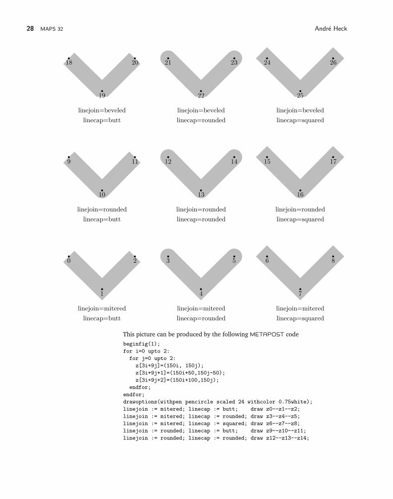
Joining LinesIn the last example of the section on pen styles you may have noticed that lines arejoined by default such that line joints are normally rounded. You can influence theappearances of the lines by the two internal variables linejoin and linecap. Thepicture below shows the possibilities.
28 MAPS 32 André Heck
0
1
2 3
4
5 6
7
8
9
10
11 12
13
14 15
16
17
18
19
20 21
22
23 24
25
26
linejoin=mitered
linecap=butt
linejoin=mitered
linecap=rounded
linejoin=mitered
linecap=squared
linejoin=rounded
linecap=butt
linejoin=rounded
linecap=rounded
linejoin=rounded
linecap=squared
linejoin=beveled
linecap=butt
linejoin=beveled
linecap=rounded
linejoin=beveled
linecap=squared
This picture can be produced by the following METAPOST code
beginfig(1);
for i=0 upto 2:
for j=0 upto 2:
z[3i+9j]=(150i, 150j);
z[3i+9j+1]=(150i+50,150j-50);
z[3i+9j+2]=(150i+100,150j);
endfor;
endfor;
drawoptions(withpen pencircle scaled 24 withcolor 0.75white);
linejoin := mitered; linecap := butt; draw z0--z1--z2;
linejoin := mitered; linecap := rounded; draw z3--z4--z5;
linejoin := mitered; linecap := squared; draw z6--z7--z8;
linejoin := rounded; linecap := butt; draw z9--z10--z11;
linejoin := rounded; linecap := rounded; draw z12--z13--z14;

Learning MetaPost by doing VOORJAAR 2005 29
linejoin := rounded; linecap := squared; draw z15--z16--z17;
linejoin := beveled; linecap := butt; draw z18--z19--z20;
linejoin := beveled; linecap := rounded; draw z21--z22--z23;
linejoin := beveled; linecap := squared; draw z24--z25--z26;
%
drawoptions();
for i=0 upto 26: dotlabel.bot(decimal(i), z[i]); endfor;
labeloffset := 25pt; label.bot("linejoin=mitered", z1);
labeloffset := 40pt; label.bot("linecap=butt", z1);
labeloffset := 25pt; label.bot("linejoin=mitered", z4);
labeloffset := 40pt; label.bot("linecap=rounded", z4);
labeloffset := 25pt; label.bot("linejoin=mitered", z7);
labeloffset := 40pt; label.bot("linecap=squared", z7);
%
labeloffset := 25pt; label.bot("linejoin=rounded", z10);
labeloffset := 40pt; label.bot("linecap=butt", z10);
labeloffset := 25pt; label.bot("linejoin=rounded", z13);
labeloffset := 40pt; label.bot("linecap=rounded", z13);
labeloffset := 25pt; label.bot("linejoin=rounded", z16);
labeloffset := 40pt; label.bot("linecap=squared", z16);
%
labeloffset := 25pt; label.bot("linejoin=beveled", z19);
labeloffset := 40pt; label.bot("linecap=butt", z19);
labeloffset := 25pt; label.bot("linejoin=beveled", z22);
labeloffset := 40pt; label.bot("linecap=rounded", z22);
labeloffset := 25pt; label.bot("linejoin=beveled", z25);
labeloffset := 40pt; label.bot("linecap=squared", z25);
%
endfig;
end;
By setting the variable miterlimit, you can influence the mitering of joints. Thenext example demonstrates that the value of this variable acts as a trigger, i.e. whenthe value of miterlimit gets smaller than some threshhold value, then the miteredjoin is replaced by a beveled value.
beginfig(1);
for i=0 upto 2:
z[3i]=(150i,0); z[3i+1]=(150i+50,-50); z[3i+2]=(150i+100,0);
endfor;
drawoptions(withpen pencircle scaled 24pt);
labeloffset:= 25pt;
linejoin := mitered; linecap:=butt;
for i=0 upto 2:
miterlimit := i;
draw z[3i]--z[3i+1]--z[3i+2];
label.bot("miterlimit=" & decimal(miterlimit), z[3i+1]);
endfor;
endfig;
end;

30 MAPS 32 André Heck
miterlimit=0 miterlimit=1 miterlimit=2
Building CyclesIn previous examples you have seen that intersection points of straight lines can bespecified by linear equations. A more direct way to deal with path intersection isvia the operator intersectionpoint. So, given four points z1, z3, z3, and z4 ingeneral position, you can specify the intersection point z5 of the line between z1and z2 and the line between z3 and z4 by
z5 = z1--z2 intersectionpoint z3--z4;
You do not need to rely on setting up linear equations with
z5 = whatever[z1,z2] = whatever[z3,z4];
The strength of the intersection operator is that it also works for curved lines.We use this operator in the next example of a filled area beneath the graph of afunction. The closed curve that forms the border of the filled area is constructedwith the buildcycle command. When given two or more paths, the buildcyclemacro tries to piece them together so as to form a cyclic path. In case there aremore intersection points between paths, the general rule is that
buildcycle(p1, p2, . . . , pn)
chooses the intersection between each pi and pi+1 to be as late as possible on thepath pi and as early as possible on pi+1. In practice, it is more convenient to choosethe path arguments such that consecutive ones have a unique intersection.
x
y
f(x)
beginfig(1);
numeric xmin, xmax, ymin, ymax;
xmin := 1/4; xmax := 6; ymax := 1/xmin; u := 1cm;
% compute the graph of the function
vardef f(expr x) = 1/x enddef;
xinc := 0.1;
path pts_f;
pts_f := (xmin,f(xmin))*u
for x=xmin+xinc step xinc until xmax:
.. (x,f(x))*u
endfor;
path hline[], vline[];
hline0 = (0,0)*u -- (xmax,0)*u;
vline0 = (0,0)*u -- (0,ymax)*u;
vline0.5 = (0.5,0)*u -- (0.5,ymax)*u;
vline4 = (4,0)*u -- (4,ymax)*u;
fill buildcycle(hline0, vline0.5, pts_f, vline4)
withcolor 0.8[blue,white];
draw hline0; draw vline0; % draw axes
draw (0.5,0)*u -- vline0.5 intersectionpoint pts_f;
draw (4,0)*u -- vline4 intersectionpoint pts_f;
draw pts_f withpen pencircle scaled 2;
label.bot(btex $x$ etex, (0.9xmax,0)*u);
label.lft(btex $y$ etex, (0,0.9ymax)*u);
label.urt(btex $f(x)$ etex, (0.5,f(0.5))*u);
endfig;
end;

Learning MetaPost by doing VOORJAAR 2005 31
EXERCISE 25 Create the following picture:
ClippingClipping is a process to select just those parts of a picture that lie inside an areathat is determined by a cyclic path and to discard the portion outside this is area.The command to do this in METAPOST is
clip picture variable to path expression;
You can use it to shade a picture element:
beginfig(1);
pair p[]; path c[];
c0 = -500*dir(40) -- 500*dir(40);
for i=0 upto 25:
draw c0 shifted (0,10*i);
draw c0 shifted (0,-10*i);
endfor;
p1 = (100,0);
c1 = (-20,0) -- (120,0);
c2 = p1--(100,infinity);
c3 = (-20,220){dir(-45)}..(120,140){right};
c4 = (0,0)--(0,infinity);
c5 = buildcycle(c1,c2,c3,c4);
clip currentpicture to c5;
p3 = c4 intersectionpoint c3;
p2 = (100, ypart p3);
draw (0,0)--p1--p2--p3--cycle;
draw c1; draw c3 withpen pencircle scaled 2;
endfig;
end;
Dealing with Paths ParametricallyIn METAPOST, a path is a continuous curve that is composed of a chain of seg-ments. Each segment is a cubic Bézier curve, which is determined by 4 controlpoints. The points on the curved segment from points p0 to p1 with post controlpoint c0 and pre control point c1 are determined by the formula
p(t) = (1 − t)3p0 + 3t(1 − t)2c0 + 3t2(1 − t)c1 + t3p1 ,
where t ∈ [0, 1]. If the path consists of two arcs, i.e., consists of three points p0,p1, and p2, then the time parameter t runs from 0 to 2. If the path consists of ncurve segments, then t runs normally from 0 to n. At t = 0 it starts at point p0 andat intermediate time t = 1 the second point p1 is reached; a third point p2 in thepath, if present, is reached at t = 2, and so on. You can get the point on a path atany time t with the construction
point t of path;
For a cyclic path with n arcs through the points p0, p1, . . . , pn−1, the normal para-meter range is 0 6 t < n, but point t of path can be computed for any t by first
32 MAPS 32 André Heck
reducing t modulo n. The number of arcs in a path is available through
length(path);
The correspondence between the time parameter and a point on the curve is alsoused to create a subpath of the curve. The command has the following syntax
subpath pair expression of path expression;
If the value of the pair expression is (t1,t2) and the path expression equals p,then the result is a path that follows p from point t1 of p to point t2 of p.If t1 > t2, then the subpath runs backward along p.
Based on the subpath operation are the binary operators cutbefore andcutafter. For intersecting paths p1 and p2,
p1 cutbefore p2;
is equivalent to
subpath(xpart(p1 intersectiontimes p2), length(p1)) of p1;
except that it also sets the path variable cuttings to the parts of p1 that gets cutoff. With multiple intersections, it tries to cut off as little as possible. Similarly,
p1 cutafter p2;
tries to cut off the part of p1 after its last intersection with p2.
We have seen that for a time parameter t we can find the corresponding pointon the curve p by the statement point t of p; Another statement, of the generalform
direction t of path;
allows you to obtain a direction vector at the point of the path that correspondswith time t. The magnitude of the direction vector is somewhat arbitrary. Thedirectiontime operation is the inverse of the direction of operation. Given adirection vector (a pair) and a path,
directiontime direction vector of path;
return a numeric value that gives the first time t when the path has the indicateddirection.
directionpoint direction vector of path;
returns the first point on the path where the given direction is achieved.
The more familiar concept of arc length is also provided for in METAPOST:
arclength(path);
returns the arc length of the given path. If p is a path and a is a number between0 and arclength(p), then
arctime a of p;
gives the time t such that
arclength(subpath(0,t) of p) = a;
A summary of the path operators is listed in the table below:

Learning MetaPost by doing VOORJAAR 2005 33
Name Arguments and Result Meaning
left right result
arclength – path numeric arc length of a path.arctime of numeric path numeric time on a path where arc length
from the start reaches a given value.cutafter path path path left argument with part after the
intersection dropped.cutbefore path path path left argument with part before the
intersection dropped.direction of numeric path path the direction of a path at a given time.directionpoint of pair path pair point where a path has a given direction.directiontime of pair path numeric time when a path has a given direction.intersectionpoint path path pair an intersection point.intersectiontimes path path numeric times (t1, t2) on paths p1 and p2
when the paths intersect.length – path numeric number of arcs in a path.point of numeric path pair point on a path given a time value.subpath pair path path portion of a path for given range of
time values times.
Let us apply what we have learned in this subsection to a couple of examples. Inthe first example, we draw a tangent line at a point of a curve.
Ti−1
Ui
Ti
beginfig(1);
path c;
c = (0,0){dir(60)}..(100,50){dir(10)};
pair p[];
p0 = point(0.1) of c;
p1 = point(0.5) of c;
p2 = point(0.9) of c;
p3 = direction(0.5) of c;
dotlabel.lrt(btex $T_{i-1}$ etex, p0);
dotlabel.lrt(btex $U_i$ etex, p1);
dotlabel.lrt(btex $T_i$ etex, p2);
draw c;
draw (-p3 -- p3) scaled (40/xpart(p3))
shifted p1;
endfig;
end;
The second example is the trefoil knot, i.e, the torusknot of type (1,3). The META-POST code has been written such that assigning n = 5 and n = 7 draws thetorusknot of type (1,5) and (1,7), respectively, in a nice way.
beginfig(1);
pair A,B; path p[];
numeric n; n:=3;
A = (0,2cm); B = A rotated (2*360/n);
p0 = A{dir(180)}..tension((n+1)/2)..
B{dir(180+2*360/n)};
numeric a;
(a,whatever) = p0 intersectiontimes
(p0 rotated (360/n));
p1 = subpath(0,a-.04) of p0;
p2 = subpath(a+.04,1) of p0;
drawoptions(withpen pencircle scaled 2);
for i=0 upto n-1:
draw p1 rotated (i*360/n);
draw p2 rotated (i*360/n);
endfor;
endfig;
end;

34 MAPS 32 André Heck
The third example shows a few steps in the Newton iterative method of findingzeros.
beginfig(1);
u := 1cm;
draw (-.5u,0)--(5u,0);
draw (0,-.5u)..(0,4u);
label.llft(btex $O$ etex, (0,0));
label.rt(btex $x$ etex, (5u,0));
label.top(btex $y$ etex, (0,4u));
Ox
y
x0x1x2
path f;
f = (.25u,-.5u){right}..(5u,4u){dir(70)};
draw f withpen pencircle scaled 1.2pt;
x0 = 4.6*u;
numeric t[];
for i=0 upto 1:
(t[i],whatever) = f intersectiontimes
((x[i],-infinity)--(x[i],infinity));
z[i] = point t[i] of f;
(x[i+1],0) = z[i] +
whatever*direction t[i] of f;
draw (x[i],0)--z[i]--(x[i+1],0);
fill fullcircle scaled 3.6pt shifted z[i];
endfor;
label.bot(btex $x_0$ etex, (x0,0));
label.bot(btex $x_1$ etex, (x1,0));
label.bot(btex $x_2$ etex, (x2,0));
endfig;
end;
EXERCISE 26 Create the following picture, which has to do with Kepler’s law of areas.
Sun
∆t∆t′
Control Structures
In this section we shall look at two commonly used control structures of imperativeprogramming languages: condition and repetition.
Conditional OperationsThe basic form of a conditional statement is
if condition: balanced tokens else: balanced tokens fi
where condition represents an expression that evaluates to a boolean value (i.e.,true or false) and the balanced tokens normally represent any valid METAPOST
statement or sequence of statements separated by semicolons. The if statement isused for branching: depending on some condition, one sequence of METAPOST
statements is executed or another. The keyword fi is the reverse of if and marksthe end of the conditional statement. The keyword fi separates the statementsequence of the preceding command clause so that the semicolon at the end ofthe last command in the else: part can be omitted. It also marks the end of the

Learning MetaPost by doing VOORJAAR 2005 35
conditional statement so that you do not need a semicolon after the keyword toseparate the conditional statement from then next statement.
Other forms of conditional statements are obtained from the basic form by:
2 Omitting the else: part when there is nothing to be said.
2 Nesting of conditional operations. The following shortcut can be used: else: ifcan be replaced by elseif, in which case the corresponding fi must be omitted.For example, nesting of two basic if operations looks as follows:
if 1st condition: 1st tokens elseif 2nd condition: 2nd tokens fi
Let us give an example: computing the centre of gravity (also called barycentre) ofa number of objects with randomly generated weight and position. The examplecontains many more programming constructs, some of which will be covered insections later on in the tutorial; so you may ignore them if you wish. The nestedconditional statement is easily found in the METAPOST code below. With thecommands numeric(x) and pair(x) we test whether x is a number or a point,respectively.
1.0579
1.39641
1.37593 0.48659
2.22429
0.73831
0.00526
0.68236
beginfig(1);
vardef centerofgravity(text t) =
save x, wght, G, X;
pair G,X; numeric wght, w;
G := origin; wght:=0;
for x=t:
if numeric(x):
show("weight = "& decimal(x));
G:= G + x*X;
wght := wght + x;
elseif pair(x):
show("location = (" &
decimal(xpart(x)) & ", " &
decimal(ypart(x)) & ")");
X:=x; % store pair
else:
errmessage("should not happen");
fi;
endfor;
G/wght
enddef;
numeric w[]; pair A[];
n:=8;
for i=1 upto n:
A[i] = 1.5cm*
(normaldeviate, normaldeviate);
w[i] = abs(normaldeviate);
dotlabel.bot(decimal(w[i]), A[i]);
endfor;
draw centerofgravity(A[1],w[1]
for i=2 upto n: ,A[i],w[i] endfor)
withpen pencircle scaled 4bp
withcolor 0.7white;
endfig;
end;
The errmessage command is for displaying an error message if something goeswrong and interrupting the program at this point. The show statement is used herefor debugging purposes. When you run the METAPOST program from a shell, showputs its results on the standard output device. In our example, the shell windowlooked like:

36 MAPS 32 André Heck
(heck@remote 1) mpost barycenter
This is MetaPost, Version 0.641 (Web2C 7.3.1)
(barycenter.mp
>> "location = (-13.14597, -80.09227)"
>> "weight = 1.0579"
>> "location = (-19.7488, -43.93861)"
>> "weight = 1.39641"
>> "location = (-43.89838, 7.07126)"
>> "weight = 1.37593"
>> "location = (-2.69252, 9.70473)"
>> "weight = 0.48659"
>> "location = (-24.17944, 25.14096)"
>> "weight = 2.22429"
>> "location = (-67.98569, -55.73247)"
>> "weight = 0.73831"
>> "location = (20.28859, -76.48691)"
>> "weight = 0.00526"
>> "location = (-67.07672, -18.69904)"
>> "weight = 0.68236" [1] )
1 output file written: barycenter.1
Transcript written on barycenter.log.
(heck@remote 2)
The boolean expression that forms the condition can be built up with the followingrelational and logical operators.
Relational Operators
Operator Meaning
= equal<> unequal< less than<= less than or equal> greater than>= greater than or equal
Logical Operators
Operator Meaning
and test if all conditions holdor test if one of many conditions holdnot negation of condition
One final remark on the use of semicolons in the conditional statement. Where thecolons after the if and else part are obligatory, semicolons are optional, dependingon the context. For example, the statement
if cycle(p): fill p;
elseif path(p): draw p;
else: errmessage("what?");
fi;
fills or draws a path depending on the path p being cyclic or not. You may omitwhatever semicolon in this example and rewrite it even as
if cycle(p): fill p
elseif path(p): draw p
else: errmessage("what?")
fi
Learning MetaPost by doing VOORJAAR 2005 37
However, when you use the conditional clause to build up a single statement, thenyou must be more careful with placing or omitting semicolons. In
draw p withcolor if cycle(p): red else: blue fi withpen pensquare;
you cannot add semicolons after the colour specifications, nor omit the final semi-colon that marks the end of the statement (unless it is a statement that is recognisedas finished because of another keyword, e.g., endfor).
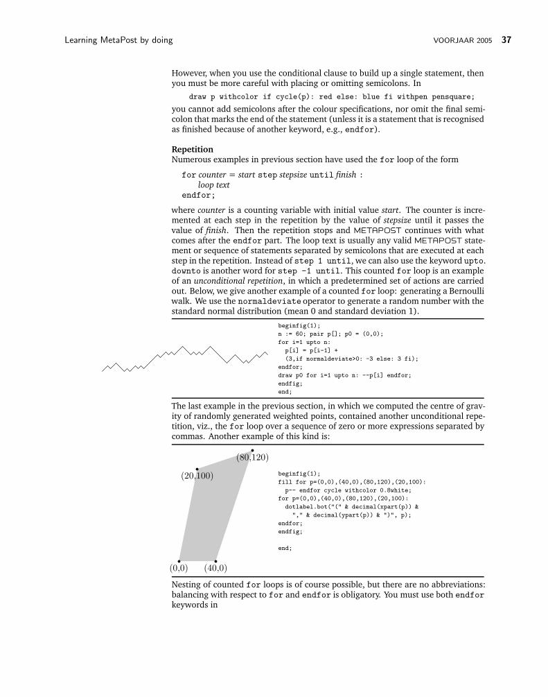
RepetitionNumerous examples in previous section have used the for loop of the form
for counter = start step stepsize until finish :loop text
endfor;
where counter is a counting variable with initial value start. The counter is incre-mented at each step in the repetition by the value of stepsize until it passes thevalue of finish. Then the repetition stops and METAPOST continues with whatcomes after the endfor part. The loop text is usually any valid METAPOST state-ment or sequence of statements separated by semicolons that are executed at eachstep in the repetition. Instead of step 1 until, we can also use the keyword upto.downto is another word for step -1 until. This counted for loop is an exampleof an unconditional repetition, in which a predetermined set of actions are carriedout. Below, we give another example of a counted for loop: generating a Bernoulliwalk. We use the normaldeviate operator to generate a random number with thestandard normal distribution (mean 0 and standard deviation 1).
beginfig(1);
n := 60; pair p[]; p0 = (0,0);
for i=1 upto n:
p[i] = p[i-1] +
(3,if normaldeviate>0: -3 else: 3 fi);
endfor;
draw p0 for i=1 upto n: --p[i] endfor;
endfig;
end;
The last example in the previous section, in which we computed the centre of grav-ity of randomly generated weighted points, contained another unconditional repe-tition, viz., the for loop over a sequence of zero or more expressions separated bycommas. Another example of this kind is:
(0,0) (40,0)
(80,120)
(20,100) beginfig(1);
fill for p=(0,0),(40,0),(80,120),(20,100):
p-- endfor cycle withcolor 0.8white;
for p=(0,0),(40,0),(80,120),(20,100):
dotlabel.bot("(" & decimal(xpart(p)) &
"," & decimal(ypart(p)) & ")", p);
endfor;
endfig;
end;
Nesting of counted for loops is of course possible, but there are no abbreviations:balancing with respect to for and endfor is obligatory. You must use both endforkeywords in

38 MAPS 32 André Heck
for i=0 upto 10:
for j=0 upto 10:
show("i = " & decimal(i) & ", j = " & decimal(j));
endfor
endfor
EXERCISE 27 Create the following picture:
EXERCISE 28 Create the picture below, which illustrates the upper and lower Riemann sum forthe area enclosed by the horizontal axis and the graph of the function f(x) = 4−x2.
EXERCISE 29 Create the following piece of millimetre paper.
EXERCISE 30 A graph is bipartite when its vertices can be partitioned into two disjoint sets A andB such that each of its edges has one endpoint in A and the other in B. The mostfamous bipartite graph is K3,3 show below to the left. Write a program that drawsthe Kn,n graph for any natural number n > 1. Show that your program indeedcreates the graph K5,5, which is shown below to the right.

Learning MetaPost by doing VOORJAAR 2005 39
a1 b1
a2 b2
a3 b3
a1 b1
a2 b2
a3 b3
a4 b4
a5 b5
Another popular type of repetition is the conditional loop. METAPOST does nothave a pre- or post conditional loop (while loop or until loop) built in. You mustcreate one by an endless loop and an explicit jump outside this loop. First theendless loop: this is created by
forever: loop text endfor;
To terminate such a loop when a boolean condition becomes true, use an exitclause:
exitif boolean expression;
When the exit clause is encountered, METAPOST evaluates the boolean expressionand exits the current loop if the expression is true. Thus, METAPOST’s version ofa until loop is:
forever:loop text;exitif boolean expression;
endfor;
If it is more convenient to exit the loop when an expression becomes false, then usethe predefined macro exitunless Thus, METAPOST’s version of a while loopis:
forever: exitunless boolean expression;loop text
endfor
Macros
Defining MacrosIn the section about the repetition control structure we introduced upto as a short-cut of step 1 until. This is also how it is is internally defined in METAPOST:
def upto = step 1 until enddef;
It is a definition of the form
def name = replacement text enddef;
It calls for a macro substitution of the simplest kind: subsequent occurrences ofthe token name will be replaced by the replacement text. The name in a macro is avariable name; the replacement text is arbitrary and may for example consist of asequence of statements separated by semicolons.
It is also possible to define macros with arguments, so that the replacement textcan be different for different calls of the macro. An example of a built-in, paramet-rised macro is:
40 MAPS 32 André Heck
def rotatedaround(expr z, d) = % rotates d degrees around z
shifted -z rotated d shifted z
enddef;
Although it looks like a function call, a use of rotatedaround expands into in-linecode. The expr in this definition means that a formal parameter (here z or d) canbe an arbitrary expression. Each occurrence of a formal parameter will be replacedby the corresponding actual argument (this is referred to as ‘call-by-value’). Thusthe line
rotatedaround(p+q, a+b);
will be replaced by the line
shifted -(p+q) rotated (a+b) shifted (p+q);
Macro parameters need not always be expressions. Another argument type is text,indicating that the parameters are just past as an arbitrary sequence of tokens.
Grouping and Local VariablesIn METAPOST, all variables are global by default. But you may want to use insome piece of METAPOST code a variable that has temporarily inside that portionof code a value different from the one outside the program block. The general formof a program block is
begingroup statements endgroup
where statements is a sequence of one or more statements separated by semicolons.For example, the following piece of code
x := 1; y := 2;
begingroup x:=3; y:=x+1; show(x,y); endgroup
show(x,y);
will reveal that the x and y values are 3 and 4, respectively, inside the programblock. But right after this program block, the values will be 1 and 2 as before.
The program block is used in the definition of the hide macro:
def hide(text t) = exitif numeric begingroup t; endgroup; enddef;
It takes a text parameter and interprets it as a sequence of statements while ulti-mately producing an empty replacement text. In other words, this command allowsyou to run code silently.
Grouping often occurs automatically in METAPOST. For example, the beginfigmacro starts with begingroup and the replacement text for endfig ends withendgroup. vardef macros are always grouped automatically, too.
You may want to go one step further: not only treating values of a variable locally,but also its name. For example, in a macro definition you may want to use a so-called local variable, i.e., a variable that only has meaning inside that definition anddoes not interfere with existing variables. In general, variables are made local bythe statement
save name sequence;
For example, the macro whatever has the replacement text8
begingroup save ?; ? endgroup
This macro returns an unknown. If the save statement is used outside of a group,the original values are simply discarded. This explains the following definition ofthe built-in macro clearxy:
8in fact, save is a vardef macro, which has the begingroup and begingroup automatically placedaround the replacement text. Thus, the begingroup and endgroup are superfluous here.

Learning MetaPost by doing VOORJAAR 2005 41
def clearxy = save x,y enddef
Vardef DefinitionsSometimes we want to return a value from a macro, as if it is a function or sub-routine. In this case we want to make sure that the calculations inside the macrodo not interfere with the expected use of the macro. This is the main purpose ofthe vardef definition of the form
def name = replacement text; returned text enddef;
By using vardef instead of def we hide the replacement text but the last statement,which returns a value.
Below we given an example of a macro that generates a random point in theregion [l,r]×[b,u]. We use the uniformdeviate to generate a random numberwith the uniform distribution between 0 and the given argument. A validity teston the actual arguments is carried out; in case a region is not defined properly, weuse errmessage to display some text and exit from the macro call, returning theorigin as default point when computing is continued.
beginfig(1);
vardef randompoint(expr l,r,b,u) =
if (r<=l) or (u<=b):
errmessage("not a proper region");
origin
else:
numeric x, y;
x = l+uniformdeviate(r-l);
y = b+uniformdeviate(u-b);
(x,y)
fi
enddef;
for i=0 upto 10:
dotlabel("",randompoint(10,100,10,100));
endfor;
endfig;
end;
Do not place a semicolon after origin or (x,y). In that case, the statement be-comes part of the hidden replacement text and an empty value is returned. Thiscauses a runtime error.
Defining the Argument SyntaxIn METAPOST, you can explicitly define the argument syntax and construct unary,binary, or tertiary operators. Let us look at the code of a predefined unary operator:
vardef unitvector primary z = z/abs z enddef;
As the example suggests, the keyword primary is enough to specify the macro asa unary vardef operator. Other keywords are secondary and tertiary. Theadvantage of specifying an n-ary operator is that you do not need to place bracketsaround arguments in compound statements; METAPOST will sort out which tokensare the arguments. For example
unitvector v rotated angle v;
is understood to be equivalent to
(unitvector(v)) rotated(angle(v));
You can also define a macro to play the role of an of operation. For example, thedirection of macro is predefined by
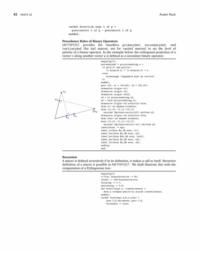
42 MAPS 32 André Heck
vardef direction expr t of p =
postcontrol t of p - precontrol t of p
enddef;
Precedence Rules of Binary OperatorsMETAPOST provides the classifiers primarydef, secondarydef, andtertiarydef (for def macros, not for vardef macros) to set the level ofpriority of a binary operator. In the example below, the orthogonal projection of avector v along another vector w is defined as a secondary binary operator.
u1
u2
2u2
u3
u4
beginfig(1);
secondarydef v projectedalong w =
if pair(v) and pair(w):
(v dotprod w) / (w dotprod w) * w
else:
errmessage "arguments must be vectors"
fi
enddef;
pair u[]; u1 = (20,80); u2 = (60,15);
drawarrow origin--u1;
drawarrow origin--u2;
drawarrow origin--2*u2;
u3 = u1 projectedalong u2;
u4 = 2*u2 projectedalong u1;
drawarrow origin--u3 withcolor blue;
draw u1--u3 dashed withdots;
draw ((1,0)--(1,1)--(0,1))
zscaled (6pt*unitvector(u2)) shifted u3;
drawarrow origin--u4 withcolor blue;
draw 2*u2--u4 dashed withdots;
draw ((1,0)--(1,1)--(0,1))
zscaled (6pt*unitvector(-u1)) shifted u4;
labeloffset := 4pt;
label.rt(btex $u_1$ etex, u1);
label.bot(btex $u_2$ etex, u2);
label.bot(btex $2u_2$ etex, 2*u2);
label.bot(btex $u_3$ etex, u3);
label.lft(btex $u_4$ etex, u4);
endfig;
end;
RecursionA macro is defined recursively if in its definition, it makes a call to itself. Recursivedefinition of a macro is possible in METAPOST. We shall illustrate this with thecomputation of a Pythagorean tree.
beginfig(1)
u:=1cm; branchrotation := 60;
offset := 180-branchrotation;
thinning := 0.7;
shortening := 0.8;
def drawit(expr p, linethickness) =
draw p withpen pencircle scaled linethickness;
enddef;
vardef tree(expr A,B,n,size) =
save C,D,thickness; pair C,D;
thickness := size;

Learning MetaPost by doing VOORJAAR 2005 43
C := shortening[B, A rotatedaround(B,
offset+uniformdeviate(branchrotation))];
D := shortening[B, A rotatedaround(B,
-offset-uniformdeviate(branchrotation))];
if n>0:
drawit(A--B, thickness);
thickness := thinning*thickness;
tree(B, C, n-1, thickness);
tree(B, D, n-1, thickness);
else:
drawit(A--B,thickness);
thickness := thinning*thickness;
drawit(B--C, thickness);
drawit(B--D, thickness);
fi;
enddef;
tree((0,0), (0,u), 10, 2mm);
endfig;
end;
EXERCISE 31 The Koch snowflake is constructed as follows: start with an equilateral triangle.Break each edge into four straight pieces by adding a bump a shown below.
You can then repeat the process of breaking a line segment into four pieces of lengthone-fourth of the segment that is broken up. Below you see the next iteration.
Write a program that can compute the picture after n iterations. After six iteration,the Koch snowflake should look like

44 MAPS 32 André Heck
Using Macro PackagesMETAPOST comes with built-in macro packages, which are nothing more than filescontaining macro definitions and constants. The most valuable macro package isgraph, which contains high-level utility macros for easy drawing graphs and dataplots. The graph package is loaded by the statement
input graph
A detailed description, including examples, of the graph package can be found in[Hob92b, GRS94]. Here, we just show one example of its use. We represent thefollowing data about the annual beer consumption in the Netherlands in the period1980–2000 graphically9.
year 1980 1985 1990 1995 2000
litre 86 85 91 86 83
Suppose that the data are stored columnwise in a file, say consumption.dat, as
1980 86
1985 85
1990 91
1995 86
2000 83
The following piece of code produces a line plot of the data. The only drawback ofthe graph package appears: years are by default marked by decade. This explainsthe densely populated labels.
1980 1990 1990 2000 2000
84
86
88
90
input graph;
beginfig(1);
draw begingraph(4cm,4cm);
gdraw "consumption.dat";
endgraph;
endfig;
end;
9Compare this example with your own code in exercise 22.
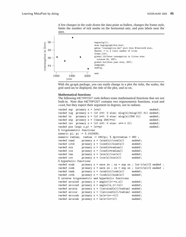
Learning MetaPost by doing VOORJAAR 2005 45
A few changes in the code draws the data point as bullets, changes the frame style,limits the number of tick marks on the horizontal axis, and puts labels near theaxes.
••
•
•
•
1980 1990 2000
84
86
88
90
year
consu
mption
inlite
rs beginfig(1);
draw begingraph(4cm,4cm);
gdraw "consumption.dat" plot btex $\bullet$ etex;
Gmarks := 3; % limit number of ticks
frame.llft;
glabel.lft(btex consumption in litres etex
rotated 90, OUT);
glabel.bot(btex year etex, OUT);
endgraph;
endfig;
end;
With the graph package, you can easily change in a plot the ticks, the scales, thegrid used an/or displayed, the title of the plot, and so on.
Mathematical functionsThe following METAPOST code defines some mathematical functions that are notbuilt-in. Note that METAPOST contains two trigonometric functions, sind andcosd, but they expect their argument in degrees, not in radians.
vardef sqr primary x = (x*x) enddef;
vardef log primary x = (if x=0: 0 else: mlog(x)/mlog(10) fi) enddef;
vardef ln primary x = (if x=0: 0 else: mlog(x)/256 fi) enddef;
vardef exp primary x = ((mexp 256)**x) enddef;
vardef inv primary x = (if x=0: 0 else: x**-1 fi) enddef;
vardef pow (expr x,p) = (x**p) enddef;
% trigonometric functions
numeric pi; pi := 3.1415926;
numeric radian; radian := 180/pi; % 2pi*radian = 360 ;
vardef tand primary x = (sind(x)/cosd(x)) enddef;
vardef cotd primary x = (cosd(x)/sind(x)) enddef;
vardef sin primary x = (sind(x*radian)) enddef;
vardef cos primary x = (cosd(x*radian)) enddef;
vardef tan primary x = (sin(x)/cos(x)) enddef;
vardef cot primary x = (cos(x)/sin(x)) enddef;
% hyperbolic functions
vardef sinh primary x = save xx ; xx = exp xx ; (xx-1/xx)/2 enddef ;
vardef cosh primary x = save xx ; xx = exp xx ; (xx+1/xx)/2 enddef ;
vardef tanh primary x = (sinh(x)/cosh(x)) enddef;
vardef coth primary x = (cosh(x)/sinh(x)) enddef;
% inverse trigonometric and hyperbolic functions
vardef arcsind primary x = angle((1+-+x,x)) enddef;
vardef arccosd primary x = angle((x,1+-+x)) enddef;
vardef arcsin primary x = ((arcsind(x))/radian) enddef;
vardef arccos primary x = ((arccosd(x))/radian) enddef;
vardef arccosh primary x = ln(x+(x+-+1)) enddef;
vardef arcsinh primary x = ln(x+(x++1)) enddef;

46 MAPS 32 André Heck
Most definitions speak for themselves, except that you may not be familiar withPythagorean addition (++) and subtraction (+-+):
++(a, b) =√
a2 + b2, + − +(a, b) =√
a2 − b2.
More Examples
The examples in this section are meant to give you an idea of the strength of META-POST.
Electronic Circuitsmpcirc is a macro package for drawing electronic circuits, developed by TomaszCholewo and downloadable from http://ci.uofl.edu/tom/software/LaTeX/mpcirc/. Let us use it to create some diagrams. We show the diagrams and thecode to create them. The basic idea of mpcirc is that you have at your disposala set of predefined electronic components such as resistor, capacity, diode, and soon. Each component has some connection points, referred to by a, b, . . ., for wires.You place the elements, using predefined orientations, and then connect them withwires. This mode of operating with mpcirc is referred to as turtle-based. Anotherprogramming style for drawing diagrams is node-based. In this approach, the nodelocations are determined first and then the elements are put between them usingbetw.x macros. We shall use the turtle-mode in our examples and hope that thecomments speak for themselves.
L
C
u:=10bp; % unit of length
input mpcirc;
beginfig(1);
prepare(L,C,Vac); % mention your elements
z0=(10u,10u); % lower right node
ht:=6u; % height of circuit
z1=z0+(0,ht); % upper right node
C=.5[z0,z1]; % location of capacitor
L.t=T.r; % use default orientation
C.t=Vac.t=T.u; % components rotated 90 degrees
% set the distance between Voltage and Capacitor
equally_spaced(5u,0) Vac, C;
L=z1-0.5(C-Vac); % location of spool
edraw; % draw components of the circuit
% draw wires connecting components
% the first ones rotated 90 degrees
wire.v(Vac.a,z0);
wire.v(Vac.b,L.a);
wire.v(L.b,z1);
wire(C.a,z0);
wire(C.b,z1);
endfig;
end;
LR Cu:=10bp; % unit of length
input mpcirc;
beginfig(1);
prepare (L,R,C,Vac); % mention your elements
z0=(0,0); % lower left node
ht:=6u; % height of circuit
z1=z0+(0,ht); % upper left node
Vac=.5[z0,z1]; % location of voltage
Vac.t=T.u; % rotated 90 degrees
L.t=R.t=C.t=T.r; % default orientation
% set equal distances
equally_spaced(5u,0) z1,R,L,C,z2;

Learning MetaPost by doing VOORJAAR 2005 47
edraw; % draw elements of circuits
% draw wires connecting nodes
% the first ones rotated 90 degrees
wire.v(Vac.a,z0);
wire.v(Vac.b,z1);
wire.v(z2,z0);
wire(z1,R.a);
wire(R.b,L.a);
wire(L.b,C.a);
wire(C.b,z2);
endfig;
end;
L
R
C
u:=10bp; % unit of length
input mpcirc;
beginfig(1);
prepare (L,R,C,Vac); % mention your elements
z0=(0,0); % lower left node
ht:=6u; % height of circuit
z1=z0+(0,ht); % upper left node
Vac=.5[z0,z1]; % location of voltage
Vac.t=T.u; % rotated 90 degrees
L.t=R.t=C.t=T.r; % default orientation
% set equal distances
equally_spaced(7.5u,0) z1,z2,z3;
L=0.5[z1,z2]; % location of spool
C=0.5[z2,z3]-(0,2u);
R=0.5[z2,z3]+(0,2u);
z4 = z3+(2.5u,0);
edraw; % draw elements of circuits
% draw wires connecting nodes
wire.v(Vac.a,z0);
wire.v(Vac.b,z1);
wire(z1,L.a);
wire(L.b,z2);
wire.v(z2,C.a);
wire.v(z2,R.a);
wire.v(z3,C.b);
wire.v(z3,R.b);
wire(z3,z4);
wire.v(z4,z0);
endfig;
end;
Marking Angles and LinesIn geometric pictures, line segments of equal length are often marked by an equalnumber of ticks and equal angles are often marked the same, too. In the followingexample, the macros tick, mark_angle, and mark_right_angle mark lines andangles. When dealing with angles, we use the macro turningnumber to find thedirection of a cyclic path: 1 means counter-clockwise, -1 means clockwise. We useit to make our macros mark_angle, and mark_right_angle independent of theorder in which the non-common points of the angle are specified.

48 MAPS 32 André Heck
A B
C
D
% set some user-adjustable constants
angle_radius := 4mm;
angle_delta := 0.5mm;
mark_size := 2mm;
def mark_angle(expr A, common, B, n) =
% draw 1, 2, 3 or 4 arcs
draw_angle(A, common, B, angle_radius);
if n>1: draw_angle(A, common, B,
angle_radius+angle_delta); fi;
if n>2: draw_angle(A, common, B,
angle_radius-angle_delta); fi;
if n>3: draw_angle(A, common, B,
angle_radius+2*angle_delta); fi;
enddef;
def draw_angle(expr endofa, common, endofb, r) =
begingroup
save tn;
tn := turningnumber(common--endofa--endofb--cycle);
draw (unitvector(endofa-common){(endofa-common)
rotated(tn*90)} .. unitvector(endofb-common))
scaled r shifted common;
endgroup
enddef;
def mark_right_angle(expr endofa, common, endofb) =
begingroup
save tn; tn :=
turningnumber(common--endofa--endofb--cycle);
draw ((1,0)--(1,1)--(0,1)) zscaled(mark_size*
unitvector((1+tn)*endofa+(1-tn)*endofb-2*common))
shifted common;
endgroup
enddef;
def tick(expr p, n) =
begingroup
save midpnt;
midpnt = 0.5*arclength(p);
% find the time when half-way the path
for i=-(n-1)/2 upto (n-1)/2:
draw_mark(p, midpnt+mark_size*i/2);
% place n tick marks
endfor;
endgroup
enddef;
def draw_mark(expr p, m) =
begingroup
save t, dm; pair dm;
t = arctime m of p;
% find a vector orthogonal to p at time t
dm = mark_size*unitvector(direction t of p rotated 90);
draw(-1/2dm..1/2dm) shifted (point t of p);
% draw tick mark
endgroup
enddef;
beginfig(1);
pair A, B, C, D;
A := (0,0); B := (3cm,0);
C := (1.5cm,4cm); D := (1.5cm,0);
draw A--B--C--cycle; draw C--D;
% draw triangle and altitude

Learning MetaPost by doing VOORJAAR 2005 49
label.bot("A", A); label.bot("B", B);
label.top("C", C); label.bot("D", D);
tick(A--D,1); tick(D--B,1); tick(A--C,2); tick(B--C,2);
mark_angle(C,A,B,2); mark_angle(A,B,C,2);
mark_angle(B,C,A,1); mark_right_angle(C,D,B);
endfig;
end;
VectorfieldsIn the first example below we show the directional field corresponding with theordinary differential equation y′ = y. For clarity, we show a vectorfield instead ofa directional field with small line segments.
x
y y = ex beginfig(1);
% some constants
numeric xmin, xmax, ymin, ymax, xinc, u;
xmin := -1.5; xmax := 1.5; ymin := 0; ymax := 4.5;
xinc := 0.05; u := 1cm;
% draw axes
draw (xmin-0.5,0)*u -- (xmax+0.5,0)*u;
draw (0,ymin-0.5)*u -- (0,ymax+0.5)*u;
% define f making up the ODE y’ = f(x,y).
% Here we take y’ = y with the exponential curve
% as solution curve
vardef f(expr x,y) = y enddef;
% define routine to compute function values
def compute_curve(suffix g)(expr xmin, xmax, xinc) =
( (xmin,g(xmin))
for x=xmin+xinc step xinc until xmax: .. (x,g(x)) endfor )
enddef;
% compute and draw exponential curve
vardef exp(expr x) = (mexp 256)**x enddef;
path p; p := compute_curve(exp, xmin, xmax, xinc) scaled u;
draw p;
% draw direction field
pair vec; path v;
for x=xmin step 0.5 until xmax:
for y=ymin+0.5 step 0.5 until ymax-0.5:
vec := unitvector( (1,f(x,y)) ) scaled 1/2u;
v := ((0,0)--vec) shifted -1/2vec;
drawarrow v shifted (x*u,y*u) withcolor blue;
endfor;
endfor;
% draw directions along the exponential curve
for x=-0.5 step 0.5 until xmax:
vec := unitvector( (1,f(x,exp(x))) ) scaled 1/2u;
v := ((0,0)--vec) shifted -1/2vec;
drawarrow v shifted (x*u,exp(x)*u) withcolor red;
endfor;
% draw ticks and labels
for x=round(xmin) upto xmax:
draw (x,-0.05)*u--(x,0.05)*u;
endfor;
for y=round(ymin) upto ymax:
draw (-0.05,y)*u--(0.05,y)*u;
endfor;
label.bot(btex $x$ etex, (xmax+0.5,0)*u);
label.lft(btex $y$ etex, (0,ymax+0.5)*u);

50 MAPS 32 André Heck
label(btex $y=eˆx$ etex, (xmax, exp(xmax)+0.5)*u);
endfig;
end;
Now we shall show some other examples of directional fields corresponding withODE’s and solution curves using the macro package courbe from Jean-MichelSarlat, which we downloaded from http://melusine.eu.org/syracuse/metapost/courbes/.
x
y
+1
+1
(x + x2)y′ − y = −1
verbatimtex
%&latex
\documentclass{article}
\begin{document}
etex
input courbes;
vardef fx(expr t) = t enddef;
vardef fy(expr t) = 1+a*t/(1+t) enddef;
beginfig(1);
repere(10cm,10cm,5cm,5cm,2cm,2cm);
trace.axes(0.5pt);
marque.unites(1mm);
%% Champs de vecteurs
vardef F(expr x,y) = (y-1)/(x+x**2) enddef;
champ.vecteurs(0.1,0.1,0.2,0.15,0.5white);
%% Courbes intégrales
color la_couleur;
la_couleur = (0.9,0.1,0.9);
for n = 0 upto 20:
a := (n/8) - 1.25;
draw ftrace(-0.995,2.5,50) en_place withcolor la_couleur;
draw ftrace(-2.5,-1.1,50) en_place withcolor la_couleur;
endfor;
%
draw rpoint(r_xmin,1)--rpoint(r_xmax,1)
withcolor la_couleur;
decoupe.repere;
etiquette.axes;
etiquette.unites;
label(btex $(x+xˆ2)y’-y=-1$ etex scaled 2.5,rpoint(0,-3));
endfig;
end;
In the next example, we added a macro to the courbes.mp package for drawing adirectional field with line segments instead of arrows.
verbatimtex
%&latex
\documentclass{article}
\begin{document}
etex
input courbes;
% ======================================== fonctions
vardef fx(expr t) = t enddef;
vardef fy(expr t) = tan(t+a) enddef;
% ======================================== figure
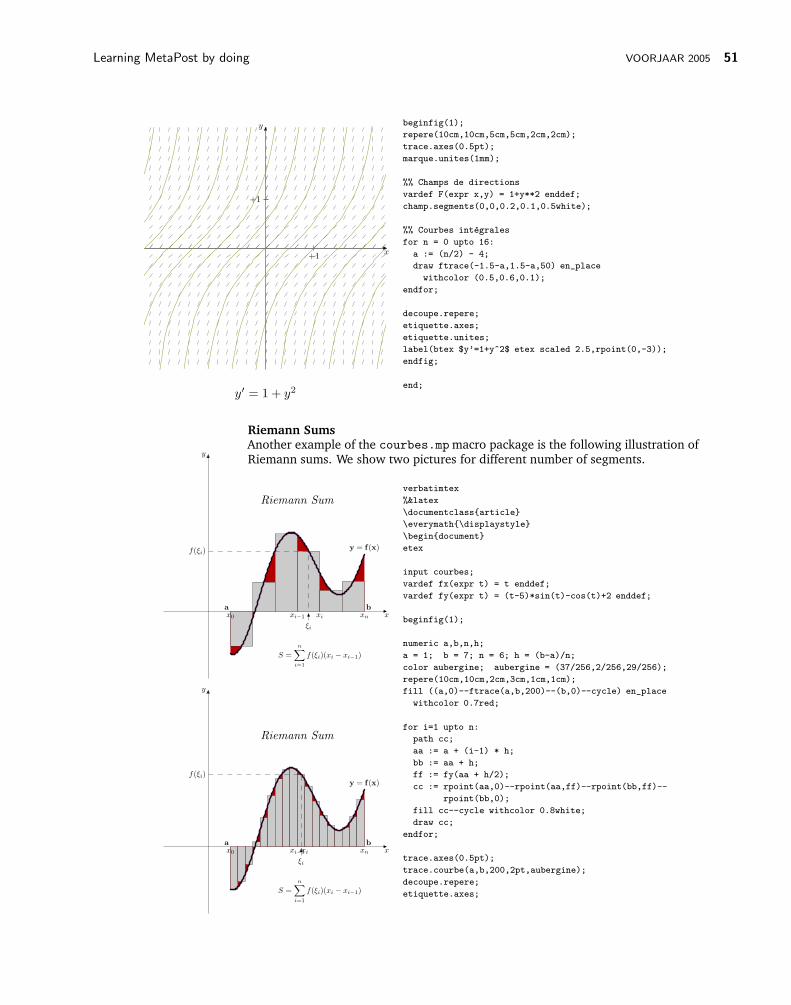
Learning MetaPost by doing VOORJAAR 2005 51
x
y
+1
+1
y′ = 1 + y2
beginfig(1);
repere(10cm,10cm,5cm,5cm,2cm,2cm);
trace.axes(0.5pt);
marque.unites(1mm);
%% Champs de directions
vardef F(expr x,y) = 1+y**2 enddef;
champ.segments(0,0,0.2,0.1,0.5white);
%% Courbes intégrales
for n = 0 upto 16:
a := (n/2) - 4;
draw ftrace(-1.5-a,1.5-a,50) en_place
withcolor (0.5,0.6,0.1);
endfor;
decoupe.repere;
etiquette.axes;
etiquette.unites;
label(btex $y’=1+yˆ2$ etex scaled 2.5,rpoint(0,-3));
endfig;
end;
Riemann SumsAnother example of the courbes.mp macro package is the following illustration ofRiemann sums. We show two pictures for different number of segments.
x
y
xi−1x0 xn
a b
y = f(x)
xi
f(ξi)
ξi
Riemann Sum
S =n∑
i=1
f(ξi)(xi − xi−1)
x
y
xi−1x0 xn
a b
y = f(x)
xi
f(ξi)
ξi
Riemann Sum
S =n∑
i=1
f(ξi)(xi − xi−1)
verbatimtex
%&latex
\documentclass{article}
\everymath{\displaystyle}
\begin{document}
etex
input courbes;
vardef fx(expr t) = t enddef;
vardef fy(expr t) = (t-5)*sin(t)-cos(t)+2 enddef;
beginfig(1);
numeric a,b,n,h;
a = 1; b = 7; n = 6; h = (b-a)/n;
color aubergine; aubergine = (37/256,2/256,29/256);
repere(10cm,10cm,2cm,3cm,1cm,1cm);
fill ((a,0)--ftrace(a,b,200)--(b,0)--cycle) en_place
withcolor 0.7red;
for i=1 upto n:
path cc;
aa := a + (i-1) * h;
bb := aa + h;
ff := fy(aa + h/2);
cc := rpoint(aa,0)--rpoint(aa,ff)--rpoint(bb,ff)--
rpoint(bb,0);
fill cc--cycle withcolor 0.8white;
draw cc;
endfor;
trace.axes(0.5pt);
trace.courbe(a,b,200,2pt,aubergine);
decoupe.repere;
etiquette.axes;
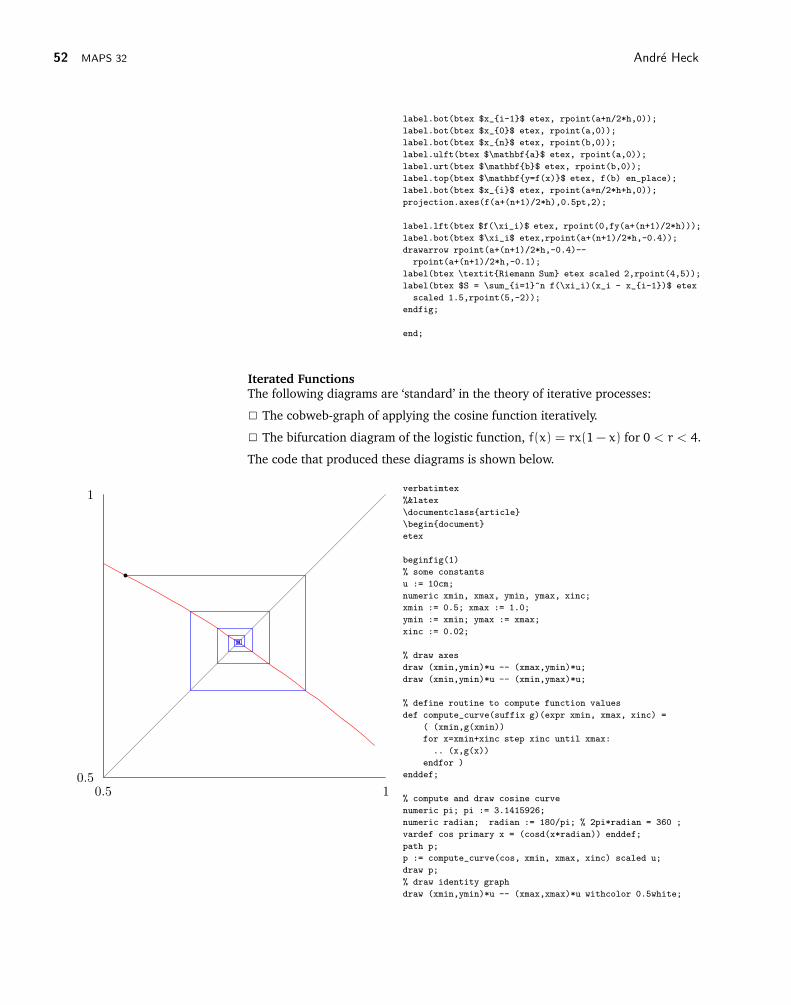
52 MAPS 32 André Heck
label.bot(btex $x_{i-1}$ etex, rpoint(a+n/2*h,0));
label.bot(btex $x_{0}$ etex, rpoint(a,0));
label.bot(btex $x_{n}$ etex, rpoint(b,0));
label.ulft(btex $\mathbf{a}$ etex, rpoint(a,0));
label.urt(btex $\mathbf{b}$ etex, rpoint(b,0));
label.top(btex $\mathbf{y=f(x)}$ etex, f(b) en_place);
label.bot(btex $x_{i}$ etex, rpoint(a+n/2*h+h,0));
projection.axes(f(a+(n+1)/2*h),0.5pt,2);
label.lft(btex $f(\xi_i)$ etex, rpoint(0,fy(a+(n+1)/2*h)));
label.bot(btex $\xi_i$ etex,rpoint(a+(n+1)/2*h,-0.4));
drawarrow rpoint(a+(n+1)/2*h,-0.4)--
rpoint(a+(n+1)/2*h,-0.1);
label(btex \textit{Riemann Sum} etex scaled 2,rpoint(4,5));
label(btex $S = \sum_{i=1}ˆn f(\xi_i)(x_i - x_{i-1})$ etex
scaled 1.5,rpoint(5,-2));
endfig;
end;
Iterated FunctionsThe following diagrams are ‘standard’ in the theory of iterative processes:
2 The cobweb-graph of applying the cosine function iteratively.
2 The bifurcation diagram of the logistic function, f(x) = rx(1 − x) for 0 < r < 4.
The code that produced these diagrams is shown below.
0.5 10.5
1verbatimtex
%&latex
\documentclass{article}
\begin{document}
etex
beginfig(1)
% some constants
u := 10cm;
numeric xmin, xmax, ymin, ymax, xinc;
xmin := 0.5; xmax := 1.0;
ymin := xmin; ymax := xmax;
xinc := 0.02;
% draw axes
draw (xmin,ymin)*u -- (xmax,ymin)*u;
draw (xmin,ymin)*u -- (xmin,ymax)*u;
% define routine to compute function values
def compute_curve(suffix g)(expr xmin, xmax, xinc) =
( (xmin,g(xmin))
for x=xmin+xinc step xinc until xmax:
.. (x,g(x))
endfor )
enddef;
% compute and draw cosine curve
numeric pi; pi := 3.1415926;
numeric radian; radian := 180/pi; % 2pi*radian = 360 ;
vardef cos primary x = (cosd(x*radian)) enddef;
path p;
p := compute_curve(cos, xmin, xmax, xinc) scaled u;
draw p;
% draw identity graph
draw (xmin,ymin)*u -- (xmax,xmax)*u withcolor 0.5white;

Learning MetaPost by doing VOORJAAR 2005 53
% compute the orbit starting from some point
numeric x, initial, orbitlength;
x := 1.0; % the starting point
initial := 1; % some initial iterations
orbitlength := 15; % number of iterations
for i=1 upto initial: % do initial iterations
x := cos(x);
endfor;
dotlabel("", (x,cos(x))*u); % mark starting point
for i=1 upto orbitlength: % draw hooks
draw (x,cos(x))*u -- (cos(x),cos(x))*u --
(cos(x),cos(cos(x)))*u withcolor blue;
x := cos(x); % next value
endfor;
% draw axis labels
labeloffset := 0.25cm;
label.bot(decimal(xmin), (xmin,ymin)*u);
label.bot(decimal(xmax), (xmax,ymin)*u);
label.lft(decimal(ymin), (xmin,ymin)*u);
label.lft(decimal(ymax), (xmin,ymax)*u);
endfig;
2.9 3.4 3.90
0.5
1
r
orb
it
beginfig(2)
numeric rmin, rmax, r, dr, n, ux, uy;
rmin := 2.9; rmax := 3.9;
r := rmin; n := 175;
dr := (rmax - rmin)/n;
ux := 8cm; uy := 8cm;
for i = 1 upto n:
x := 0.5; % our starting point
for j=1 upto 75: % initial iterations
x := r*x*(1-x);
endfor
for j=1 upto 150: % the next 100 iterations
x := r*x*(1-x);
draw (r*ux,x*uy) withpen pencircle scaled .5pt;
endfor
r := r+dr;
endfor;
% draw axes and labels
draw (rmin*ux,0) -- (rmax*ux,0);
draw (rmin*ux,0) -- (rmin*ux,uy);
labeloffset := 0.25cm;
label.bot(decimal(rmin), (rmin*ux,0));
label.bot(decimal((rmin+rmax)/2), ((rmin+rmax)/2*ux,0));
label.bot(decimal(rmax), (rmax*ux,0));
label.lft(decimal(0), (rmin*ux,0));
label.lft(decimal(0.5), (rmin*ux,0.5*uy));
label.lft(decimal(1), (rmin*ux,uy));
label.bot(btex $r$ etex, ((rmax-0.2)*ux,0));
label.lft(btex orbit etex rotated 90, (rmin*ux,0.75*uy));
endfig;
end;

54 MAPS 32 André Heck
A Surface PlotYou can draw surface plots from basic principles. We give one example.
X
Y
Z
z = cos(xy)
verbatimtex
%&latex
\documentclass{article}
\begin{document}
etex
% u: dimensional unit
% xp, yp, zp: coordinates of light source
% bf : brightness factor
% base_color : base color
numeric u,xp,yp,zp,bf;
color base_color;
u = 1cm;
xp := 3; yp := 3; zp := 5;
bf := 30;
base_color := red+green;
% O, Xr, Yr, Zr : reference frame
pair O,Xr,Yr,Zr;
O = (0,0);
Xr = (-.7,-.7) scaled u;
Yr = (1,0) scaled u;
Zr = (0,1) scaled u;
% for drawing the reference frame
vardef frameXYZ(expr s) =
drawarrow O--Xr scaled s;
drawarrow O--Yr scaled s;
drawarrow O--Zr scaled s;
label.llft(btex $X$ etex scaled 1.25, (Xr scaled s));
label.rt(btex $Y$ etex scaled 1.25, (Yr scaled s));
label.top(btex $Z$ etex scaled 1.25, (Zr scaled s));
enddef;
% from 3D to 2D coordinates
vardef project(expr x,y,z) = x*Xr + y*Yr + z*Zr enddef;
% numerical derivatives by central differences
vardef diffx(suffix f)(expr x,y) =
numeric h; h := 0.01;
(f(x+h,y)-f(x-h,y))/(2*h)
enddef;
vardef diffy(suffix f)(expr x,y) =
numeric h; h := 0.01;
(f(x,y+h)-f(x,y-h))/(2*h)
enddef;
% Compute brightness factor at a point
vardef brightnessfactor(suffix f)(expr x,y,z) =
numeric dfx,dfy,ca,cb,cc;
dfx := diffx(f,x,y);
dfy := diffy(f,x,y);
ca := (zp-z)-dfy*(yp-y)-dfx*(xp-x);
cb := sqrt(1+dfx*dfx+dfy*dfy);
cc := sqrt((z-zp)*(z-zp)+(y-yp)*(y-yp)+(x-xp)*(x-xp));
bf*ca/(cb*cc*cc*cc)
enddef;
% compute the colors and draw the patches
vardef
z_surface(suffix f)(expr xmin,xmax,ymin,ymax,nx,ny) =
numeric dx,dy,xt,yt,zt,factor[][];
pair Z[][];

Learning MetaPost by doing VOORJAAR 2005 55
dx := (xmax-xmin)/nx;
dy := (ymax-ymin)/ny;
for i=0 upto nx:
xt := xmin+i*dx;
for j=0 upto ny:
yt := ymin+j*dy;
zt := f(xt,yt);
Z[i][j] = project(xt,yt,zt);
factor[i][j] := brightnessfactor(f,xt,yt,zt);
endfor
endfor
for i = 0 upto nx-1:
for j= 0 upto ny-1:
fill Z[i][j]--Z[i][j+1]--Z[i+1][j+1]--Z[i+1][j]--cycle
withcolor factor[i][j]*base_color;
endfor
endfor
enddef;
beginfig(1);
xp := 3;
yp := 3;
zp := 10;
bf := 100;
numeric pi; pi := 3.14159;
vardef cos primary x = cosd(x/pi*180) enddef;
vardef f(expr x,y) = cos(x*y) enddef;
z_surface(f,-3,3,-3,3,100,100);
frameXYZ(5);
label(btex $z = \cos(xy)$ etex scaled 1.25,(0,-4cm));
endfig;
end;
MiscellaneousWe adopt another example from Jean-Michel Sarlat that uses his macro packagecourbe and another one called grille. The example has been downloaded andslightly adapted from http://melusine.eu.org/syracuse/metapost/cours/sarlat/derivation/.
a x
f(a)
f(x)
A
f(x) − f(a)
x − af ′(a)
graph of f
Derivative at a point
x
y verbatimtex
%&latex
\documentclass{article}
\begin{document}
etex
input courbes;
input grille;
vardef droite(expr a,b,t) =
(t[a,b])--(t[b,a])
enddef;
path c,cartouche;
c=(2.3cm,1cm)..(4.5cm,4cm)..(9cm,3cm);
cartouche = (3cm,2mm)--(7cm,2mm)--(7cm,8mm)--(3cm,8mm)--
cycle;
pair A,M;
A = point 0.6 of c;
M = point 1.5 of c;
vardef tangente(expr t,x) =
pair X,Y;
X := point (t-.05) of c;
Y := point (t+.05) of c;

56 MAPS 32 André Heck
droite(X,Y,x)
enddef;
beginfig(1);
grille(1cm,0,10cm,0,7cm);
repere(10cm,7cm,2cm,2cm,1cm,1cm);
trace.axes(.5pt);
marque.unites(0.1);
%% lectures sur la grille
numeric xa,ya,xm,ym;
xa = 1.25; ya = 1.1 ; xm = 4.9 ; ym = 2.25;
pair AA,MM;
AA = (xa,ya) ; MM = (xm,ym) ;
projection.axes(AA,0.5,1.7);
projection.axes(MM,0.5,1.7);
label.bot(btex $a$ etex,rpoint(xa,0));
label.bot(btex $x$ etex,rpoint(xm,0));
label.lft(btex $f(a)$ etex, rpoint(0,ya));
label.lft(btex $f(x)$ etex, rpoint(0,ym));
%% fin des lectures
draw c withpen pencircle scaled 1.5pt withcolor (.2,.4,.9);
draw droite(A,M,1.2);
draw tangente(0.6,9) withpen pencircle scaled 1.5pt;
dotlabel.ulft(btex $A$ etex scaled 1.5,A);
dotlabel("",M);
label(btex $\displaystyle\frac{f(x)-f(a)}{x-a}$ etex
scaled 1.25,
M shifted (1cm,1cm));
label.ulft(btex $f’(a)$ etex scaled 1.25, (5cm,5cm));
label.bot(btex graph of $f$ etex scaled 1.25, point 2 of c);
%% Cartouche
fill cartouche withcolor .8white;
draw cartouche;
label.rt(btex \textbf{Derivative at a point}
etex,(3cm,5mm));
%% fin du cartouche
decoupe.repere;
etiquette.axes;
endfig;
end;
References
[ GRS94 ] Michel Goossens, Sebastian Rahtz, Frank Mittelbach. The LaTEXGraphics Companion, Addison-Wesley (1994), ISBN 0-201-85469-4.
[ Hag02 ] Hans Hagen. The Metafun Manual, 2002. downloadable aswww.pragma-ade.com/general/manuals/metafun-p.pdf
[ Hob92a ] John D. Hobby: A User’s manual for MetaPost, AT&T BellLaboratories Computing Science Technical Report 162, 1992.
[ Hob92b ] John D. Hobby: Drawing Graphs with MetaPost, AT&T BellLaboratories Computing Science Technical Report 164, 1992.