lattice boltzmann methods for flows of complex fluids ... · edward lewis lattice boltzmann methods...
TRANSCRIPT

Lattice Boltzmann Methods for Flows of Complex Fluids
Edward Lewis
Supervised by Prof. T.N. Phillips
A thesis presented for the degree of
Doctor of Philosophy
School of Mathematics
Cardiff University
United Kingdom
2017

Acknowledgements
Firstly I would like to thank my supervisor, Professor Tim Phillips, for his time,
care and understanding throughout the time I have been at Cardiff University.
His advice and guidance has always been very useful and gratefully received
and our frequent meetings is something I am going to miss on completion of my
studies. I would also like to thank Cardiff University’s School of Mathematics
for providing such a stimulating academic environment. The people in the
department provide that extra bit of inspiration and joy on a cold wet winter
Welsh morning. Finally, I would like to thank my family and my fiancee for
their love, support and gracious understanding. It is difficult to imagine how
I could have done this without them.
I

Declaration
This work has not previously been accepted in substance for any degree and
is not concurrently submitted in candidature for any degree.
Signed.......................................Date........................
Statement 1
This thesis is being submitted in partial fulfilment of the requirements for the
degree of PhD.
Signed.............................. Date.................................
Statement 2
This thesis is the result of my own independent work/investigation, except
where otherwise stated. Other sources are acknowledged by explicit
references.
Signed............................... Date.................................
Statement 3
I hereby give consent for my thesis, if accepted, to be available for
photocopying and for inter-library loan, and for the title and summary to be
made available to outside organisations.
Signed............................... Date.................................
Statement 4
I hereby give consent for my thesis, if accepted, to be available for
photocopying and for inter-library loans after expiry of a bar on access
approved by the Graduate Development Committee.
Signed............................... Date.................................
II

Abstract
This thesis presents the extension of the lattice Boltzmann method (LBM) to
the solution of the Fokker-Planck equation with the FENE force law, on a single
lattice for the use of modelling the flows of polymeric liquids. First implemen-
tation and the basic theory of the LBM is discussed including the derivation
of the equilibrium function as a discretisation of the Maxwell-Boltzmann dis-
tribution function using Gauss-Hermite quadrature and the recovery of the
Navier-Stokes equations from the LBE by use of multiscale analysis. A review
of the extension of the LBM to multiphase flow is presented including colour
models, pseudo-potential models and free energy models. Numerical results
for a colour model have been given. Current viscoelastic lattice Boltzmann
methods are discussed including results validating the approach by Onishi et
al. [75] in the cases of simple shear flow and start up shear flow. A LBM for
the Fokker-Planck equation with the FENE force law is developed based on a
new Gauss quadrature rule that has been derived. The validity of this method
is confirmed for small We by comparison with results by Ammar [2] and Singh
et al. [96] where it gives good agreement. A LBM for the Fokker-Planck equa-
tion is then coupled with a macroscopic solver for the solvent velocity to solve
start-up plane Couette flow. This approach is validated by comparison with
results by Leonenko and Phillips [60].
III

Contents
1 Introduction 1
1.0.1 Finite Difference methods . . . . . . . . . . . . . . . . . 1
1.0.2 Finite Volume methods . . . . . . . . . . . . . . . . . . . 2
1.0.3 Finite Element methods . . . . . . . . . . . . . . . . . . 3
1.1 Different Modelling Approaches . . . . . . . . . . . . . . . . . . 7
1.2 The Lattice Gas Cellular Automaton . . . . . . . . . . . . . . . 13
1.3 From LGCA to LBM . . . . . . . . . . . . . . . . . . . . . . . . 17
1.4 Overview of the Lattice Boltzmann Model . . . . . . . . . . . . 19
2 The Lattice Boltzmann Method: Implementation 23
2.1 Collision Algorithm . . . . . . . . . . . . . . . . . . . . . . . . . 23
2.2 Propagation Algorithm . . . . . . . . . . . . . . . . . . . . . . . 27
2.3 Boundary Conditions . . . . . . . . . . . . . . . . . . . . . . . . 28
2.4 Body Forces . . . . . . . . . . . . . . . . . . . . . . . . . . . . . 32
2.5 Numerical Results . . . . . . . . . . . . . . . . . . . . . . . . . . 32
2.6 Discussion . . . . . . . . . . . . . . . . . . . . . . . . . . . . . . 36
3 Lattice Boltzmann Theory 37
3.1 From the Continuum Boltzmann Equation to the Lattice Boltz-
mann Equation . . . . . . . . . . . . . . . . . . . . . . . . . . . 37
3.2 Derivation of the Equilibrium Distribution Function . . . . . . . 42
3.3 Relation Between the Lattice Boltzmann Method and Navier-
Stokes . . . . . . . . . . . . . . . . . . . . . . . . . . . . . . . . 46
3.4 Discussion . . . . . . . . . . . . . . . . . . . . . . . . . . . . . . 50
IV

Edward Lewis Lattice Boltzmann Methods for Flows of Complex Fluids V
4 Multiphase fluid flows 51
4.1 Surface Tension . . . . . . . . . . . . . . . . . . . . . . . . . . . 52
4.2 Chromodynamic models . . . . . . . . . . . . . . . . . . . . . . 54
4.3 The pseudo-potential approach . . . . . . . . . . . . . . . . . . 55
4.4 The free energy approach . . . . . . . . . . . . . . . . . . . . . . 58
4.5 Mean field model . . . . . . . . . . . . . . . . . . . . . . . . . . 59
4.6 Numerical Results . . . . . . . . . . . . . . . . . . . . . . . . . . 66
4.7 Poiseuille Flow . . . . . . . . . . . . . . . . . . . . . . . . . . . 71
4.8 Discussion . . . . . . . . . . . . . . . . . . . . . . . . . . . . . . 73
5 Lattice Boltzmann methods for droplets 75
5.1 Numerical implementation of wetting boundary condition . . . . 76
5.2 Discussion . . . . . . . . . . . . . . . . . . . . . . . . . . . . . . 83
6 LBM for viscoelastic fluids 85
6.1 What are viscoelastic fluids? . . . . . . . . . . . . . . . . . . . . 85
6.2 Mathematically modelling viscoelastic fluids . . . . . . . . . . . 86
6.2.1 Linear Viscoelasticity . . . . . . . . . . . . . . . . . . . . 86
6.2.2 Constitutive equations derived from microstructures . . . 88
6.3 Viscoelastic Lattice Boltzmann methods . . . . . . . . . . . . . 94
6.3.1 A lattice Boltzmann method for the Jeffreys model . . . 95
6.3.2 Lattice Fokker-Planck Equation . . . . . . . . . . . . . . 99
6.4 Discussion . . . . . . . . . . . . . . . . . . . . . . . . . . . . . . 108
7 LBM for FENE model 112
7.1 A LBM for FENE fluids . . . . . . . . . . . . . . . . . . . . . . 114
7.1.1 Kinetic theory description of the Fokker-Planck equation
for FENE dumbbells . . . . . . . . . . . . . . . . . . . . 114
7.1.2 Discrete kinetic model for FENE dumbbells . . . . . . . 116
7.1.3 Coupling with LBM . . . . . . . . . . . . . . . . . . . . 125
7.1.4 Lattice Boltzmann method for polymer kinetic theory . . 127
7.1.5 Numerical Results . . . . . . . . . . . . . . . . . . . . . 133
7.1.6 Discussion . . . . . . . . . . . . . . . . . . . . . . . . . . 136
8 Conclusions and future Work 144

Chapter 1
Introduction
The lattice Boltzmann method (LBM) is an algorithm for simulating the flows
of fluids. Conventional numerical schemes, such as finite difference, finite el-
ements and finite volumes, rely on discretising macroscopic continuum equa-
tions. However, the LBM is a discrete kinetic theory approach that features a
mescoscale description of the microstructure of the fluid.
The most commonly used macroscopic continuum equations used in fluid
dynamics are the Navier-Stokes equations
ρDu
Dt= −∇P + η∇2u + ρb, (1.0.1)
∇ · u = 0. (1.0.2)
where u is the macroscopic fluid velocity, ρ is the fluid density, P is the fluid
pressure, η is the dynamic viscosity, b is body force (e.g. gravity) and the
material derivative is given by
D
Dt=
∂
∂t+ u · ∇. (1.0.3)
1.0.1 Finite Difference methods
In finite difference methods, differential equations are approximated with dif-
ference equations, in which finite differences approximate the derivatives. For
example, first we need to define a grid of points in the domain D = [a, b]×[c, d].
We choose step sizes ∆x = b−aN
and ∆y = d−cM
in the x and y directions, re-
1

2
spectively (where N and M are integers) and a time step size ∆t. We draw a
set of horizontal and vertical lines across D, and get a set of intersection points
(xi, yj, tn), or simply (i, j, n), where xi = a+ i∆x, i = 0, . . . , N, yj = a+ j∆y,
j = 0, . . . ,M, and tn = n∆t. Then using first order forward difference for time
discretisation, first order backwards difference for first order space derivative
and second order central difference for second order space derivative, the com-
ponent of the momentum equation in the x-direction is given by
un+1ij − unij
∆t+ unij
unij − uni−1,j
∆x+ vnij
unij − uni−1,j
∆y
= −1
ρ
pni+1,j − pni−1,j
2∆x+ η
(uni+1,j − 2unij + uni−1,j
∆x2+uni,j+1 − 2unij + uni,j−1
∆y2
)where unij is the velocity in the x direction at the point (i, j, n). Finite differ-
ence methods have a few drawbacks. For hyperbolic systems, the differential
equations do not hold at discontinuities, whereas the integral conservation laws
do and in practice finite difference methods require structured meshes making
simulating the flow around complex geometries (such as flow through porous
media) very difficult to implement.
1.0.2 Finite Volume methods
Finite volume methods are similar to finite difference methods in that values
are calculated at discrete points on a meshed geometry. The basis of the fi-
nite volume method is the integral conservation law. The essential idea is to
divide the domain into many control volumes and approximate the integral
conservation law on each of the control volumes. Because the flux entering a
given volume is identical to that leaving an adjacent volume, these methods
are conservative. Finite volume methods are also easily formulated to allow
for unstructured meshes. Beginning with the incompressible form of the mo-
mentum equation divided through by the density (p = P/ρ) and density has
been absorbed into the body force term fi
∂ui∂t
+∂ui∂uj∂xj
= − ∂p
∂xi+ ν
∂2ui∂xj∂xj
+ fi. (1.0.4)

Edward Lewis Lattice Boltzmann Methods for Flows of Complex Fluids 3
The equation is integrated over the control volume of a computational cell∫ ∫ ∫V
[∂ui∂t
+∂ui∂uj∂xj
]dV =
∫ ∫ ∫V
[− ∂p
∂xi+ ν
∂2ui∂xj∂xj
+ fi
]dV (1.0.5)
The time dependent term and the body force term are assumed to be constant
over the volume of the cell. The divergence theorem is applied to remaining
terms to give
∂ui∂tV +
∫ ∫A
uiujnjdA = −∫ ∫
A
pnidA+
∫ ∫ν∂ui∂xj
njdA+ fiV (1.0.6)
where n is the normal of the surface of the control volume and V is the volume.
Usually polyhedra are used as control volumes and values are assumed constant
over each face, and so the area integrals can be written as summations over
each face
∂ui∂tV +
∑nbr
(uiujnjA)nbr = −∑nbr
(pniA)nbr+∑nbr
(ν∂ui∂xj
njA
)nbr
+fiV (1.0.7)
where the subscript nbr denotes the value at any given face.
1.0.3 Finite Element methods
The finite element method again formulates the problem in terms of a system
of algebraic equations. The method yields approximate values of the unknowns
at discrete number points over the domain. To solve the problem, it subdi-
vides the computational domain into a number of finite elements. The simple
equations that model these finite elements are then assembled into a larger
system of equations that model the entire problem. FEM then uses varia-
tional methods to approximate a solution by minimizing an associated error
function.
For example, we consider the two dimensional steady flow problem in a
domain Ω where the fluid velocity u = 0 at the boundary Γ. The formulation

4
of our example is now. For x ∈ Ω solve u satisfying
div u = 0, (1.0.8)
− div σ + ρ(u · ∇u) = ρb, (1.0.9)
σij = −Pδij + T (1.0.10)
u = 0 for x ∈ Γ. (1.0.11)
where T is the deviatoric extra stress tensor. Define the solution space for u
as
V = H1E(Ω) =
v :
∫Ω
(v(x))2dΩ +
∫Ω
|∇v(x)|2dΩ ≤ C1, v = 0 on Γ
.
(1.0.12)
and the solution space for P as
Q = HE(Ω) =
q :
∫Ω
(q(x))2dΩ ≤ C2
. (1.0.13)
In order to derive the weak formulation, equations (1.0.8) and (1.0.9) must be
multiplied by test functions that belong to the solution space. First equation
(1.0.8) is multiplied by a test function q and integrated over Ω which yields∫Ω
q div udΩ = 0. (1.0.14)
The momentum equations (1.0.9) consist of two equations (one for the x and
y directions), which are each multiplied by separate test functions v1 and v2
and then integrated over Ω. By defining v = (v1, v2)† these equations can be
combined to ∫Ω
(− div σ + ρ(u · ∇u)) · vdΩ =
∫Ω
b · vdΩ. (1.0.15)
The first term in (1.0.15) is further reduced by applying integration by parts
(Divergence theorem) to∫Ω(− divΣ) · vdΩ =
∫Ω
σ · ∇vdΩ−∫
Γ
n · σ · vdΓ (1.0.16)

Edward Lewis Lattice Boltzmann Methods for Flows of Complex Fluids 5
where n is the outward pointing unit normal vector. Furthermore by substi-
tuting equation (1.0.10) into (1.0.16), the first term of (1.0.15) may be written
as ∫Ω(− divΣ) · vdΩ =
∫Ω
T · ∇vdΩ +
∫Ω
P div vdΩ−∫
Γ
n · σ · vdΓ
(1.0.17)
Combining these results leads to the weak formulation of the Navier-Stokes
equations. Find u ∈ V and P ∈ Q with
u = 0 at Γ, (1.0.18)
such that ∫Ω
q div udΩ = 0, (1.0.19)∫Ω
T · ∇vdΩ +
∫Ω
ρ(u · ∇u) · vdΩ−∫
Ω
P div vdΩ =
∫Ω
ρb · vdΩ, (1.0.20)
for all v such that v = 0 at Γ, Ω is the fluid domain boundary, Γ is the
boundary of Ω and T is the deviatoric extra stress tensor. We see that no
derivatives of P and q are necessary and so it is sufficient that P and q are
integrable. For u and v, first derivatives are required and hence not only u
and v but also their first derivatives must be integrable.
In the standard Galerkin method we define a basis function Ψi(x) for the
pressure components and functions Φij(x) for the vector components (Φi1 and
Φi2 for the x and y directions). Now the approximation of u and P will be
defined by
ph =m∑j=1
pjΨj(x) (1.0.21)
uh =n∑j=1
u1jΦj1(x) + u2jΦj2(x) =2n∑j=1
ujΦj(x). (1.0.22)
In equation (1.0.22) uj is defined by uj = u1j (j = 1, . . . , n), uj+n = u2j
(j = 1, . . . , n) and Φj in the same way. In order to get the standard Galerkin

6
formulation we substitute v = Φi(x), q = Ψi(x) into the weak formulation. In
this way we get, find ph and uh defined by equations (1.0.21,1.0.22) such that∫Ω
Ψi div uhdΩ = 0, i = 1, . . . ,m (1.0.23)
and ∫Ω
T · ∇ΦidΩ +
∫Ω
ρ(uh · ∇uh) · ΦidΩ (1.0.24)
−∫
Ω
P div ΦidΩ =
∫Ω
ρb · ΦidΩ, i = 1, . . . ,m. (1.0.25)
The finite element method may be used to construct the basis functions Φi
and Ψi and once they are known the integrals (1.0.23) and (1.0.25) may be
evaluated element-wise. This produces a system of m+2n non-linear equations
with m + 2n unknowns. The solution of the system of equations introduces
two difficulties, firstly the equations are non-linear so require an iterative solver
and secondly the equations resulting from the mass equation do not contain
the unknown pressure P . For a finite element problem to be well-posed it is
necessary that the test spaces satisfy the well known LBB condition. In general
finite element methods are very amenable to unstructured meshes but are
more difficult to formulate and implement when compared to finite difference
schemes.
With the LBM the aim is to construct simplified kinetic type models that
preserve the conservation laws (e.g. mass, momentum) and necessary symme-
tries (e.g. Galilean invariance) so that in the macroscopic limit, the macro-
scopic averaged properties obey the desired continuum equations of motion,
such as the Navier-Stokes equations. These simplified models are sufficient
since the macroscopic dynamics are not sensitive to the underlying details of
the microscopic physics.
The LBM developed in the late 1980s has seen rapid development and is
now being used for many applications such as heat convection in buildings [54],
blood coagulation in a human artery [4] and modelling of fluid turbulence [19].

Edward Lewis Lattice Boltzmann Methods for Flows of Complex Fluids 7
1.1 Different Modelling Approaches
People have been interested in the world around them for thousands of years
but it is only in the last few centuries that we have started to quantify physical
phenomena. The physics of fluids is very complicated and for all but the
simplest of flows is poorly understood. With the rise of computing power it
has been possible to start to model fluids numerically. Traditionally scientists
have modelled fluids at a continuum scale, where fluids are described in terms of
space filling fields, such as density, velocity, and pressure, that vary smoothly in
space and time. Such a description is fairly adequate for many applications, to
the point that the physics of fluids is often implicitly identified with continuum
fluid mechanics. Nevertheless, it has been known for over a century, that fluids
(gas and liquids) are ultimately composed of a collection of individual entities,
atoms and molecules, whose discrete nature becomes apparent at scales around
the nanometre and below.
The different levels of description have an associated characteristic length
scale. At the macroscopic level there may be a number of such lengths such
as the width of a channel or the diameter of an object in the flow. These
are examples of geometric lengths but more intrinsic flow properties like the
diameter of a vortex shed in turbulent flow may also be considered. Denote
the smallest of the hydrodynamic length scales by LH . At the particle, or
microscopic scale, the characteristic length scale is generally taken to be the
mean free path, Lmfp, which is the average distance particles travel between
collisions. A basic hypothesis underlying continuum fluid mechanics is that
the macroscopic description holds whenever LH Lmfp, or alternatively
ε =LmfpLH
1, (1.1.1)
where ε is known as the Knudsen number.
For a purely microscopic approach we consider a collection of N particles
of mass m moving in a volume V at time t, each with position vector xi,
i = 1, . . . , N . Let each particle move freely under the influence of a force Fi.

8
The particles are described by the Hamiltonian equations of motion:
dxidt
=jim, (1.1.2)
djidt
= Fi (1.1.3)
where ji is the momentum of particle i. If initial conditions and boundary
conditions are specified, the Hamiltonian equations can, in principle, be solved
in time to give full knowledge of the state of the system. However, the number
of particles N in V is large. In fact, it is typically very large indeed. If we
had a 1 m3 box full of air at room temperature, we would have roughly 1025
particles. This is why simply solving the Hamiltonian equations is an infeasible
task in practice.
The macroscopic approach does not consider the internal structure of V
but instead considers it to be an arbitrary material volume fixed in space with
a density ρ and a momentum which is assumed to satisfy the conservation laws
of Newtonian mechanics so that
d
dt
∫V
ρdV = 0, (1.1.4)
d
dt
∫V
ρudV =
∫S
n · σdS +
∫V
ρbdV, (1.1.5)
where u is the fluid velocity, σ is a stress tensor, S is the surface of V with
outward normal n and b is a body force (such as gravity). Applying the di-
vergence and Reynolds transport theorems yields, under the assumptions that
all integrands are continuous and the fluid is incompressible, the macroscopic
equations of motion for a fluid are
∇ · u = 0, (1.1.6)
ρDu
Dt= ∇ · σ + ρb, (1.1.7)
whereD
Dt=
∂
∂t+ u · ∇ (1.1.8)
is the material derivative. To derive an explicit form of the stress tensor we

Edward Lewis Lattice Boltzmann Methods for Flows of Complex Fluids 9
write the components σαβ of σ in the form
σαβ = −Pδαβ + Tαβ, (1.1.9)
where δαβ is the usual Kronecker delta function and T is the deviatoric extra
stress tensor. Define P , the pressure, to be the negative average of the diagonal
stress components, i.e.
P = −1
3Tr σ. (1.1.10)
A constitutive equation is needed to model the extra stress tensor T to
close the system of equations. This can take many forms depending on the
type of fluid that is to be modelled. For a Newtonian fluid it is assumed that
the extra stress tensor is proportional to the rate of strain γ i.e.
T = ηγ, (1.1.11)
where η, is known as the viscosity and the rate of strain tensor is defined to
be
γ = ∇u + (∇u)†, (1.1.12)
and † denotes the matrix transpose. With T defined in (1.1.11), the Navier-
Stokes equations can be recovered
ρDu
Dt= −∇P + η∇2u + ρb, (1.1.13)
∇ · u = 0. (1.1.14)
This forms a continuum model that assumes the underlying physical sys-
tem is smoothly varying, in contrast to physical fluids which are actually com-
posed of a fixed number of discrete particles. The Navier-Stokes equations
(1.1.13), (1.1.14) are highly nonlinear and analytic solutions are rarely avail-
able. Therefore, numerical solutions become necessary and traditionally this
has been achieved through finite volume or finite element methods (local meth-
ods) or spectral elements (global method). For many real life problems, such
as the aerodynamic properties of cars or weather forecasting, these techniques
have proved to be very successful, especially in predicting qualitative behaviour
of fluid flows. However there are some potential issues which can cause com-

10
putational difficulties. For example, there may be truncation errors and nu-
merical instabilities due to the necessary discretisation process, irregular fluid
domain boundaries which are difficult to incorporate (in particular with the
finite volume method), a Poisson solver is often required to solve for the pres-
sure (which is computationally expensive), issues with the ill-posedness of the
discrete problem caused by possible incompatibilty between the approximation
spaces (finite and spectral element methods), the nonlinearity of the Navier-
Stokes equations and for multiphase flows, the interface between the two fluids
has to be tracked in time (which is not easily achieved by continuum-based
methods). For non-Newtonian fluids that have a complex constitutive equa-
tion for the stress, care must be taken to avoid extra numerical instabilities
and spurious oscillations when dealing with the convective term, u · ∇T.
Modern computing architectures are driving the demand for CFD tech-
niques that are amenable to parallel computing. There are two main issues
with producing an algorithm suitable for parallel computing,
(i) the fraction of parallel content
(ii) the load balance.
To illustrate (i), suppose we were given the task of summing N numbers.
We could get P processors to sum a fraction of the numbers each but there
is a serial bottleneck when it comes to summing these P partial sums. An
algorithm with many such bottlenecks will not work well on parallel computers.
The benefit (S(P )) of using P processors, where W is the fraction of work that
can be performed in parallel is given in [100] by
S(P ) =1
W/P + (1−W ). (1.1.15)
This equation shows that in the limit of an infinite number of processors, the
speed up asymptotes to S(∞) = 1/(1−W ). As an example suppose we have
ninety percent parallel code, the above equation shows that the maximum pay
off will never exceed a factor of 10. Therefore 10 processors is approximately
the threshold above which further parallelisation becomes wasteful. For ref-
erence large scale LBM easily place more than 99 percent of the computer
demand on the collision phase which is perfectly parallel [100] giving scope for
Edward Lewis Lattice Boltzmann Methods for Flows of Complex Fluids 11
the use of more than 100 processors.
Load balancing, (ii) refers to making sure each processor is doing roughly
the same amount of work, as computational speed can be limited by the speed
of the slowest processor. With regular geometries, load balancing is a trivial
matter, where a simple geometric domain decomposition assures good perfor-
mance. When the geometry is complex and possibly even changing in time it
is difficult a priori to know how to ensure each processor is performing even ap-
proximately the same amount of work. LBM has a simple data structure and
so is well positioned to steer clear of load balancing issues for many practical
applications.
A third intermediate level of description is provided by kinetic theory. This
connects the small scale (Lmfp) microscopic picture with the large scale (LH)
macroscopic properties. Kinetic theory considers a statistical description of
the fluid microstructure and defines the physical observables (e.g. density, ve-
locity, temperature, pressure) to be averages over a large number of molecular
histories. The primary variable in kinetic theory is not the position of a parti-
cle or the macroscopic velocity, but instead the distribution function, f(x, ξ, t),
which is defined to be the probability of finding a particle at position x with
velocity ξ at time t.
In 1872 Ludwig Boltzmann devised the famous Boltzmann equation which
describes the statistical behaviour of a thermodynamic system not in thermo-
dynamic equilibrium which reads
∂tf + ξ · ∇f = Ω(f) (1.1.16)
where f = f(x, ξ, t) is the single particle distribution function, ξ is the mi-
croscopic velocity, and Ω(f) is a collision operator, so that f(x, ξ, t)d3xd3ξ is
the probability of finding a particle in the volume d3x around x with velocity
between ξ and ξ + dξ.
The macroscopic variables are determined from the moments of the distri-

12
bution function
ρ(x, t) =
∫f(x, ξ, t)dξ, (1.1.17)
ρ(x, t)u(x, t) =
∫ξf(x, ξ, t)dξ, (1.1.18)
ρ(x, t)e(x, t) =
∫(ξ − u)2f(x, ξ, t)dξ, (1.1.19)
where ρ is the fluid density, u is the fluid velocity and e is the internal energy,
the energy contained within the system excluding the kinetic and potential
energy of the system as a whole.
The collision operator Ω(f) is very complicated and suitable approxima-
tions need to be constructed to make the LBE amenable to numerical com-
putations. The assumption behind many simplifications to Ω is that a large
amount of information about the two-body interactions is unlikely to influence,
to a great extent, the values of experimentally measured quantities.
Cercignani [12] showed that the collision integral possesses exactly five
elementary collision invariants ψk(c), k = 0, . . . , 4, i.e.∫Ω(f, f)ψk(c)dc = 0. (1.1.20)
These are
ψ0 = 1, (ψ1, ψ2, ψ3) = c, ψ4 = c2. (1.1.21)
Simpler collision operators should also satisfy this constraint as well as the
tendency to a Maxwellian distribution (H-theorem) [81]. The most commonly
chosen approximation to the collision operator is the Bhatnagar-Gross-Krook
(BGK) operator [5]
Ω(f) = −1
λ(f − f eq) (1.1.22)
which represents a simplified description of a particle’s relaxation to a local
equilibrium state due to collisions. In equation (1.1.22), λ is the relaxation
time (characteristic time taken to relax to the equilibrium solution) due to
collisions and f eq is the Boltzmann-Maxwellian distribution function
f eq =ρ
(2πRT )D/2exp
(−(ξ − u)2
2RT
), (1.1.23)

Edward Lewis Lattice Boltzmann Methods for Flows of Complex Fluids 13
where R is the ideal gas constant, D is the dimension of physical space, and ρ,
u and T are the macroscopic density, velocity and temperature, respectively.
This simplified model does have some disadvantages as the relaxation time
simultaneously controls the fluid viscosity and the discretisation errors. Solu-
tions obtained with the BGK model generally exhibit λ-dependent and there-
fore viscosity-dependent characteristics. Thus the fundamental physical re-
quirement that hydrodynamic solutions are uniquely determined by their non-
dimensional physical parameters is not satisfied [53] (p. 143).
The connection between kinetic theory and hydrodynamics is provided
by multiscale analysis, which separates the different spatial and temporal
scales within a fluid. This is done using Chapman-Enskog analysis on Boltz-
mann’s equation (1.1.16) which allows one to derive the Navier-Stokes equa-
tions (1.1.13) and (1.1.14).
1.2 The Lattice Gas Cellular Automaton
In 1986, Frisch, Hasslacher and Pomeau [30] showed that a simple cellular
automaton (commonly called FHP after the authors’ initials) which obeyed
only simple conservation laws at a microscopic level, was able to reproduce the
complexity of real fluid flows. This was the subject of great excitement in the
CFD community. The prospects were promising: a round-off free, intrinsically
parallel computational paradigm for fluid flow and perhaps, even more im-
portantly the analogue of the Ising model for turbulence [100]. A few serious
problems (such as statistical noise and amenability to three dimensions) were
quickly recognised and the Lattice Boltzmann Equation (LBE) was developed
in its wake as a response to some of drawbacks of LGCA [45]. LBE is now
viewed as its own self-standing research subject in its own right and it can be
derived independently, without reference to LGCA at all. However, it is still
useful to start with a brief overview of LGCA as it aids our understanding of
the LBE.
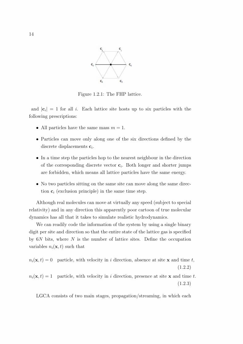
The FHP lattice, which is shown in Figure 1.2.1, is a regular lattice with
hexagonal symmetry and associated with each node are the six link vectors
defined by
ci =
(cos
iπ
3, sin
iπ
3
), i = 1, . . . , 6, (1.2.1)
14
Figure 1.2.1: The FHP lattice.
and |ci| = 1 for all i. Each lattice site hosts up to six particles with the
following prescriptions:
• All particles have the same mass m = 1.
• Particles can move only along one of the six directions defined by the
discrete displacements ci.
• In a time step the particles hop to the nearest neighbour in the direction
of the corresponding discrete vector ci. Both longer and shorter jumps
are forbidden, which means all lattice particles have the same energy.
• No two particles sitting on the same site can move along the same direc-
tion ci (exclusion principle) in the same time step.
Although real molecules can move at virtually any speed (subject to special
relativity) and in any direction this apparently poor cartoon of true molecular
dynamics has all that it takes to simulate realistic hydrodynamics.
We can readily code the information of the system by using a single binary
digit per site and direction so that the entire state of the lattice gas is specified
by 6N bits, where N is the number of lattice sites. Define the occupation
variables ni(x, t) such that
ni(x, t) = 0 particle, with velocity in i direction, absence at site x and time t,
(1.2.2)
ni(x, t) = 1 particle, with velocity in i direction, presence at site x and time t.
(1.2.3)
LGCA consists of two main stages, propagation/streaming, in which each

Edward Lewis Lattice Boltzmann Methods for Flows of Complex Fluids 15
Figure 1.2.2: The collision rules on the FHP lattice. The numbers on the openarrows are the transition probabilities. The most common choice for p is 0.5
particle hops to one of its nearest neighbours according to its momentum, and
collision in which particles entering the same lattice site interact and change
their momentum according to a set of pre-determined collision rules (in practice
this is done by use of a look-up table).
The LGCA evolution can now be described by the equation
ni(x + ci, t+ 1)− ni(x, t) = Ωi(n) (1.2.4)
where Ωi is the collision operator that acts on all particles n = ni : i =
1, . . . , 6. The collision operator Ωi must conserve mass and momentum, i.e.∑i
Ωi = 0, (1.2.5)∑i
Ωici = 0. (1.2.6)
In the HPP model the collision phase is deterministic whereas the FHP model
features a partially stochastic process. If there is a head-on two body collision
then the incoming particles will rotate by either +π3
or −π3
with probabilities
p and 1− p, respectively. Examples are shown in Figure 1.2.2.

16
In order to calculate macroscopic quantities such as density and momen-
tum, we first start by averaging ni over a small subdomain x in some suitable
manner to reduce the statistical noise associated with LGCA. The region in
which spatial averaging takes place must be small compared to a typical macro-
scopic length scale of the flow. The mean occupation numbers Ni are then used
to calculate the macroscopic density, momentum and momentum flux tensor
defined, respectively, by
ρ(x, t) =∑
Ni(x, t) (1.2.7)
ρ(x, t)uα(x, t) =∑
Ni(x, t)ciα (1.2.8)
Παβ(x, t) =∑
Ni(x, t)ciαciβ (1.2.9)
where uα is the α component of velocity u. Rivet and Boon [87] have shown
that the FHP lattice gas, can give rise to the full equations of motion for a
real isotropic fluid.
Despite the elegance and practical appeal of round-off-free parallel com-
puting, LGCA are plagued by a number of anomalies, such as statistical noise
(common to any particle method) and broken symmetries which cannot be
restored even in the limit of zero lattice spacing [21].
One such problem is encountered when we move into the third dimension.
The only regular polytope that fills the whole space is the cube, while the
only regular polytopes with a sufficiently large symmetry group are the do-
decahedron and icosahedron. There is an elegant solution to this problem,
d’Humieres et al.[26] showed that a suitable lattice could be found by going
into the fourth dimension. They showed that the Face Centred HyperCube
(FCHC) has the correct properties. It consists of all neighbours of a given site
(the central site) generated by the speeds ci = [±1,±1, 0, 0] and permutations
thereof. This yields 24 speeds all with the same magnitude c2i = 2.
If we examine the lattice (Figure 1.2.3) we see that the neighbours in the
centre of a face are represented by two particles corresponding to the ±1 in
the fourth dimension. Although it solves the problem of isotropy in the third
dimension, it dramatically increases the computational complexity. This was
a decisive factor in the move from LGCA to LBM.

Edward Lewis Lattice Boltzmann Methods for Flows of Complex Fluids 17
Figure 1.2.3: The face centered hypercubic lattice.
1.3 From LGCA to LBM
The Lattice Boltzmann Model (LBM) can be viewed as a direct extension of
LGCA developed by researchers such as McNamara and Zanetti [69] to resolve
some of the shortcomings of LGCA. The occupation variable ni is replaced
by the average population density fi(x, t) = 〈ni(x, t)〉. Taking the ensemble
average of the LGCA evolution equation (1.2.4) leads to the non-linear LBE
fi(x + ci, t+ 1) = fi(x, t) + 〈Ωi(n)〉. (1.3.1)
To obtain a kinetic equation in closed form Boltzmann’s assumption that
particles entering a collision are uncorrelated is used
fi(x + ci, t+ 1) = fi(x, t) + Ωi(f), (1.3.2)
where f = [f1, . . . , fb]. In the lattice Boltzmann framework, the macroscopic
density and momentum are defined by the zeroth and first moments of the

18
distribution function, respectively:
ρ =∑i
fi, (1.3.3)
ρu =∑i
fici. (1.3.4)
This solved some issues such as statistical noise but still had difficulties in
three dimensions, a lack of Galilean invariance and a relatively high viscosity
and therefore low Reynolds number barrier (due to the maximum number of
collisions an automaton can support) [84].
The next major breakthrough was by Higuera and Jimenez [45] who con-
quered the exponential complexity limitation by considering perturbations of
the local equilibrium function. The macrostates of the LBM are functions of
the space variable x and vary slowly in space. Any significant variation takes
place over distances much larger than the lattice length scale. We can say that
the population distribution function departs slightly from the local equilibrium
state and write
fi = f(0)i + εf
(1)i + ε2f
(2)i + . . . , (1.3.5)
where f(0)i = f eqi is the equilibrium state and the expansion parameter (Knud-
sen number) ε 1 is the ratio of the microscopic scale to the smallest macro-
scopic scale.
The equilibrium component is required to fulfil the following constraints
b∑i=1
f eqi = ρ, (1.3.6)
b∑i=1
f eqi ci = ρu. (1.3.7)
Upon inserting fi into the collision term and expanding in a Taylor series about
the equilibrium component we get
Ωi(fi) ≈ Ω(0)i + ε
∑j
∂Ω(0)i
∂fjf
(1)j +
ε2
2
∑jk
∂2Ω(0)i
∂fj∂fkf
(1)j f
(1)k , (1.3.8)
where Ω(0)i = Ωi(f
(0)i ). This equation can be simplified since Ωi(f
(0)i ) = 0 and

Edward Lewis Lattice Boltzmann Methods for Flows of Complex Fluids 19
by the conservation of momentum∂Ω
(0)i
∂fjf
(1)j = 0 [84], so that we obtain the
quasi-linear lattice Boltzmann equation
fi(x + ci, t+ 1)− fi(x, t) =∑j
Mij
(fj − f eqj
), (1.3.9)
where Mij =∂Ω
(0)i
∂fj, defines the collision matrix which determines the scattering
rate between directions i and j. The importance of this procedure is that it
reduces the complexity of the collision term from 2b to b2 and then, due to
the symmetry of Mij, to order b, thus making it computationally feasible to
perform lattice Boltzmann simulations in three dimensions.
The viscosity of the LB fluid is entirely controlled by a single parameter,
namely the leading nonzero eigenvalue of the scattering matrix Mij [100]. The
remaining eigenvalues are then chosen to improve stability. This raises the
question that since transport is related to a single nonzero eigenvalue, why not
simplify things and choose a one parameter scattering matrix? Many authors
[16, 52, 82] raised this point simultaneously and defined the Lattice Bhatnagar
Gross Krook (LBGK) model
fi(x + ci, t+ 1)− fi(x, t) = ω(fj − f eqj
), (1.3.10)
where ω, which is the first nonzero eigenvalue of Mij, is a relaxation param-
eter. The LBGK model is the simplest and most efficient LBM that recovers
the Navier-Stokes equations and is probably the most widely used due to its
simplicity and ease of implementation.
1.4 Overview of the Lattice Boltzmann Model
The LBM simplifies Boltzmann’s original idea of gas dynamics by reducing the
number of particles and confining them to the nodes of a lattice. Although it is
entirely possible to perform lattice Boltzmann simulations on the FHP lattice
with additional ‘rest’ velocity, most simulations are now performed on square
lattices. The common notation used for describing lattices used in LBM is
DmQn where m is the number of dimensions and n is the number of velocities.
The advantages of square lattices include greater accuracy due to the increased

20
Figure 1.4.1: The D2Q9 Lattice
number of discrete velocity vectors [97], the ease of implementation and their
amenability to three dimensional problems. To give a brief overview of the
lattice Boltzmann method we shall discuss the D2Q9 model, which is two
dimensional and consists of nine discrete velocity vectors. Figure 1.4.1 shows
a typical lattice node of the D2Q9 model with nine velocities ci defined by
ci =
(0, 0) i = 0
(−1, 1), (−1, 0), (−1,−1), (0,−1) i = 1, 2, 3, 4
(1,−1), (1, 0), (1, 1), (0, 1) i = 5, 6, 7, 8
(1.4.1)
where ci = −ci+4 for i = 1, 2, 3, 4, as this makes coding easier.
We associate a discrete probability distribution function fi(xi, ci, t) or sim-
ply fi(xi, t) i = 0, . . . , 8, which describes the probability of streaming in one
particular direction. We can then discretise (1.1.16) to obtain
fi(x + ci∆t, t+ ∆t)− fi(x, t)︸ ︷︷ ︸streaming
= Ωi︸︷︷︸collision
. (1.4.2)
where the key steps in LBM are the streaming (or propagation) and colli-
sion processes. When implementing the model the collision and propagation
(streaming) steps are computed separately, and attention must be paid when
applying boundary conditions since some types have to applied after the colli-
sion step and some after the propagation step. For example the on-grid bounce
back boundary condition is applied after the propagation step but the mid-grid
bounce back boundary condition is applied after the collision step.

Edward Lewis Lattice Boltzmann Methods for Flows of Complex Fluids 21
The macroscopic fluid density, momentum and internal energy can be de-
fined by moments of the microscopic particle distribution function,
ρ(x, t) =8∑i=0
fi(x, t), (1.4.3)
ρ(x, t)u(x, t) =8∑i=0
cifi(x, t), (1.4.4)
ρ(x, t)e(x, t) =8∑i=0
(ci − u)2fi(x, t), (1.4.5)
The equilibrium component (to be discussed in more detail in Chapter 3)
to which the distribution function relaxes, is required to fulfil the following
constraints:
ρ(x, t) =8∑i=0
f eqi (x, , t), (1.4.6)
ρ(x, t)u(x, t) =8∑i=0
cifeqi (x, t). (1.4.7)
When using the on-grid bounce-back boundary condition (which will be
discussed in the next chapter), the algorithm can be summarized as follows:
1. Initialize ρ, u, fi and f eqi
2. Collision step: calculate the updated distribution functions
3. Propagation step: move fi → f ∗i in the direction of ci
4. Compute the post propagation boundary conditions (if applicable)
5. Compute macroscopic ρ and u from f ∗i using the moment equations
6. Compute f eqi using the equilibrium equation
7. Advance time and repeat steps 2 to 7 until the stopping criteria are
satisfied. For example a specified end time or convergence to a steady
state solution.

22
In the case where mid-grid bounce-back condition is used, the boundary
condition is computed after the collision step rather than after the propagation
step.

Chapter 2
The Lattice Boltzmann Method:
Implementation
In this chapter we will explore in greater depth different aspects of the LBM
and how one would implement the algorithm in practice.
2.1 Collision Algorithm
When constructing simpler collision operators it has been common to use one
of two different methods based on either a single relaxation time or multiple
relaxation times. Single relaxation time methods tend to be faster and easier
to implement and multiple relaxation times tend to be more stable.
BGK single relaxation time
A simplified collision model that satisfies the necessary constraints is the BGK
(Bhatnagar, Gross Krook) approximation [5]:
Ω(f) = ω(f eq − f), (2.1.1)
where f now relaxes towards f eq with a single relaxation time τf = 1/ω where
ω is the collision frequency. This gives rise to the LBGK equation
fi(x + ci∆t, t+ ∆t)− fi(x, t) = − 1
τf(fi(x, t)− f eqi (x, t)). (2.1.2)
23

24
From the study of the literature we see that the lattice form of the BGK
is the most commonly used collision operator due to the ease with which it
can be implemented. However due to the use of a single relaxation time the
method does suffer from stability issues unless 0 < τf < 2. Since there is a
single relaxation time it means that the bulk ν ′ and kinematic ν viscosities
are linearly proportional [23]. The use of a single relaxation time means that
heat transfer takes place at the same rate as momentum transfer. Therefore the
Prandtl number is always unity and so the LBGK equation is only appropriate
for isothermal flows.
Multiple Relaxation Time (MRT)
The lattices commonly used in applications contain more distribution functions
than necessary to reproduce the fluid density, momentum, and stress that ap-
pear in the Navier-Stokes equations. The additional degrees of freedom are
required for isotropy, but are detrimental to stability. A Multiple-Relaxation-
Time (MRT) or matrix collision operator is constructed to over-relax the stress
alone. The remaining variables (non physical) are damped towards equilib-
rium, leading to substantial gains in stability.
MRT collision schemes are applied to the moments for each lattice point
rather than the distribution functions [49, 56]. The moments and distribution
functions which are related to each other by
M = T f (2.1.3)
where f is a vector of allm distribution functions for the point, i.e. (f0, f1, ..., f8)†,
M the vector of moments (also the size of the number of discrete lattice speeds
and dependent on the lattice system) and T the transformation matrix that
renders the moments in terms of the distribution functions. Equilibrium values
for the moments Meq, can be determined by transforming the standard local
equilibrium functions into moment space by
Meq = T f eq, (2.1.4)
where f eq is the vector of local equilibrium distribution functions. The resulting
equilibrium moments can alternatively be expressed directly as functions of

Edward Lewis Lattice Boltzmann Methods for Flows of Complex Fluids 25
fluid density and velocity. Certain moments, such as density and momentum,
must be conserved and their equilibrium values are set so that no changes
are made. The post-collisional moments are determined by relaxation of the
non-equilibrium part, i.e.
M(x, t+ ∆t) = M(x, t)− Λ(M(x, t)−Meq(x, t)) (2.1.5)
where Λ is the collision matrix, which takes the form of a diagonal matrix of
collision parameters (again the same size as the number of discrete velocities
of the lattice used), which we represent by the vector s so that
Λ = diag(s). (2.1.6)
Some of the collision parameters can be specified to set both kinematic
and bulk viscosities, a few others can be tuned to improve simulation stability
and the remainder are fixed (as previously stated) to conserve macroscopic
hydrodynamics. Setting all the values of s (the diagonal entries of Λ) to 1τf
reduces the scheme to the BGK single relaxation time collision model.
Since the collision matrix is diagonal, equation (2.1.5) can be rewritten in
terms of each moment, i.e.
Mi(x, t+ ∆t) = Mi(x, t)− si(Mi(x, t)−Meqi (x, t) (2.1.7)
Multiplying Mi(x, t + ∆t) by the inverse of the transformation matrix, T−1,
gives the post-collisional distribution functions.
An example is given for the D2Q9 lattice system; the moment vector is
M = (ρ, e, ε, jx, qx, jy, qy, pxx, pxy)† (2.1.8)
with ρ as the density, e the energy, ε the square of energy, j momentum, q
energy flux, pxx the diagonal stress tensor component and pxy the off-diagonal
stress tensor component. The transformation matrix is
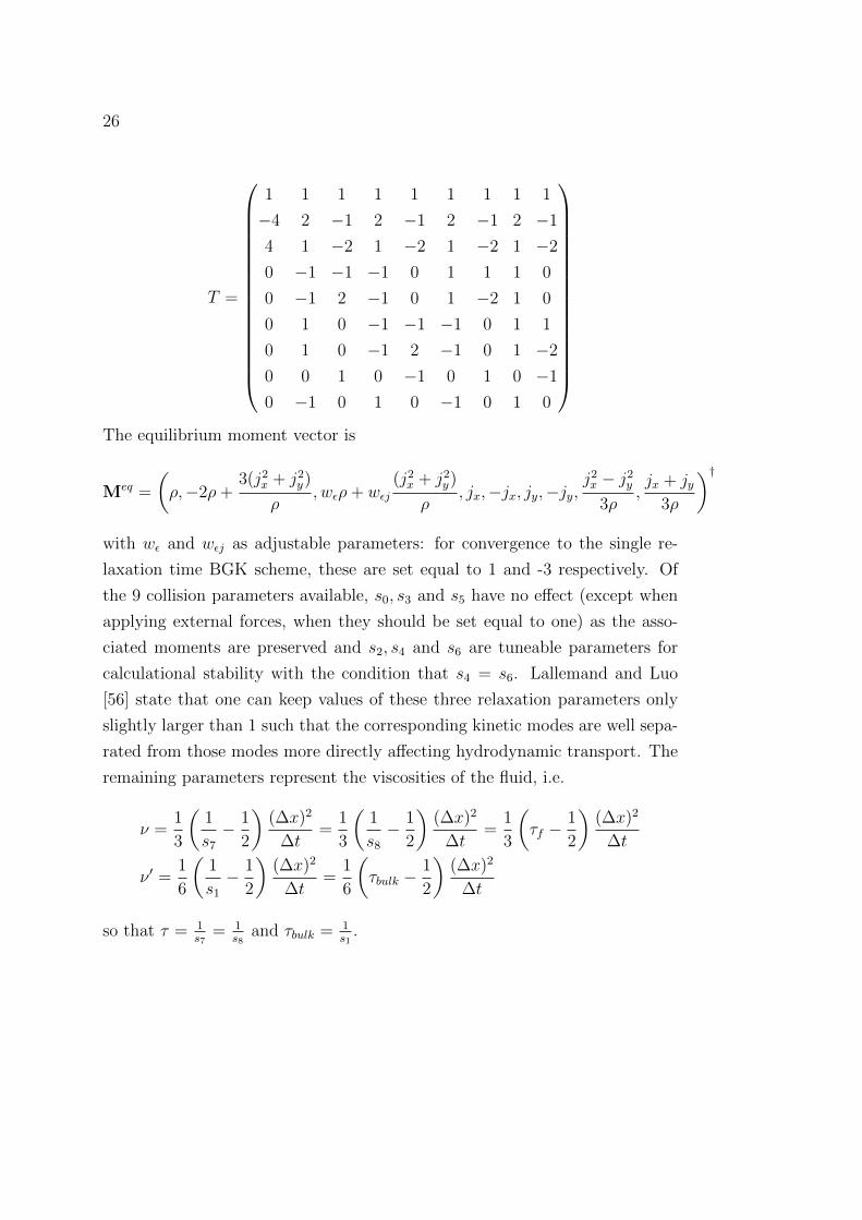
26
T =
1 1 1 1 1 1 1 1 1
−4 2 −1 2 −1 2 −1 2 −1
4 1 −2 1 −2 1 −2 1 −2
0 −1 −1 −1 0 1 1 1 0
0 −1 2 −1 0 1 −2 1 0
0 1 0 −1 −1 −1 0 1 1
0 1 0 −1 2 −1 0 1 −2
0 0 1 0 −1 0 1 0 −1
0 −1 0 1 0 −1 0 1 0
The equilibrium moment vector is
Meq =
(ρ,−2ρ+
3(j2x + j2
y)
ρ, wερ+ wεj
(j2x + j2
y)
ρ, jx,−jx, jy,−jy,
j2x − j2
y
3ρ,jx + jy
3ρ
)†with wε and wεj as adjustable parameters: for convergence to the single re-
laxation time BGK scheme, these are set equal to 1 and -3 respectively. Of
the 9 collision parameters available, s0, s3 and s5 have no effect (except when
applying external forces, when they should be set equal to one) as the asso-
ciated moments are preserved and s2, s4 and s6 are tuneable parameters for
calculational stability with the condition that s4 = s6. Lallemand and Luo
[56] state that one can keep values of these three relaxation parameters only
slightly larger than 1 such that the corresponding kinetic modes are well sepa-
rated from those modes more directly affecting hydrodynamic transport. The
remaining parameters represent the viscosities of the fluid, i.e.
ν =1
3
(1
s7
− 1
2
)(∆x)2
∆t=
1
3
(1
s8
− 1
2
)(∆x)2
∆t=
1
3
(τf −
1
2
)(∆x)2
∆t
ν ′ =1
6
(1
s1
− 1
2
)(∆x)2
∆t=
1
6
(τbulk −
1
2
)(∆x)2
∆t
so that τ = 1s7
= 1s8
and τbulk = 1s1
.

Edward Lewis Lattice Boltzmann Methods for Flows of Complex Fluids 27
2.2 Propagation Algorithm
The simplest implementation involves the use of a temporary array to copy
post-collisional distribution functions to their new positions, which are subse-
quently copied back to the main distribution function array. This method is
clear, easy to understand and can be applied throughout the system’s lattice
points in any order, its drawbacks include the use of two loops for propagation
and array copying, two large arrays for distribution functions at each lattice
node and significant amounts of time expended in memory access.
An alternative, more memory efficient implementation of propagation is
the swap algorithm detailed in [68], in which this process is performed by the
systematic swapping of pairs of collided distribution function values. To make
this easier to implement, the lattice links are organised so that the conjugate
link j to link i (i.e. cj = −ci) is equal to i + m−12
for i = 1, . . . , m−12
(where
m is number of discrete velocities of the lattice model). Looping i between 1
and m−12
the post-collisional distribution functions for each lattice point fi(x)
are initially swapped with their conjugate values fj(x), then at each point the
value fj(x) is then swapped with fi(x + ci∆t).
These sets of swaps can be carried out either in two separate steps or in one
go. The use of separate swap steps requires two sweeps through the domain,
but the order in which distribution functions are swapped does not matter
and no boundary domain is necessary for serial calculations. Simultaneous
swapping cannot make use of automatic periodic boundary conditions and
requires lattice links to be additionally ordered so that the first half are directed
to lattice points that have previously gone through at least the first swap stage,
but only a single sweep through the domain is required.
The two array method when implemented efficiently could be significantly
faster on modern computer architectures as there are fewer read and writes to
memory which for large systems can take a significant time. There is a trade
off between speed and memory usage and this may depend on the particular
application.

28
2.3 Boundary Conditions
To apply boundary conditions to a Lattice Boltzmann Equation simulation,
the distribution functions fi at boundary lattice points have to be modified or
replaced during each time step to give the required fluid velocity or pressure.
This may take place either between the collision and propagation stages or at
the end of each time step. The easy implementation of boundary conditions
is a massive advantage for LBM, making LBM an ideal numerical method for
the simulation of fluid flows in complicated geometries, such as flow through
porous media. Here are some examples of simple boundary conditions.
Periodic
Periodic boundaries are used to simulate bulk fluids sufficiently far away from
the actual boundaries of a real physical system so that surface effects can be
neglected. As the fluid moves out of one face of the system volume it reappears
on the opposite face with the same velocity, density etc.
Bounce-back
This boundary condition evolved from the bounce back condition of LGCA.
The bounce-back condition applies a no-slip condition at a boundary. This
is applied after the propagation stage by reversing the distribution functions
sitting on each wall node xw, i.e.
fi(xw, t) = fj(xw, t) (2.3.1)
where j is the conjugate lattice link to i, i.e. cj = −ci. The reflection of
distribution functions occurs on-grid and this is shown in Figure 2.3.1. On-
grid bounce-back is a first order approximation of the boundary condition
(error is proportional to lattice spacing), but it is completely local.
Ziegler [105] realised that a second-order bounce back scheme can be used if
the boundary lies between two lattice grid lines and this is illustrated in Figure
2.3.2. This method essentially applies the actual reflection halfway between
timesteps and is a spatially second-order method.
The bounce-back condition is accurate and easy to implement when the
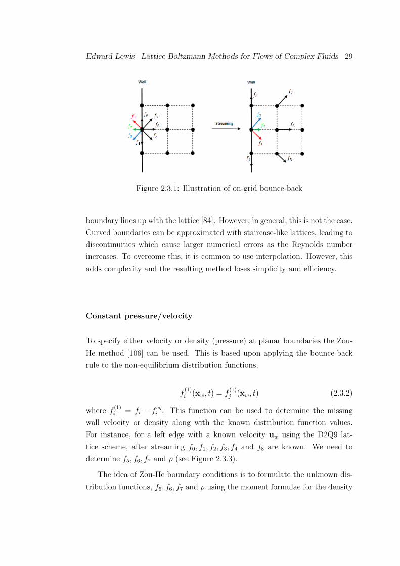
Edward Lewis Lattice Boltzmann Methods for Flows of Complex Fluids 29
Figure 2.3.1: Illustration of on-grid bounce-back
boundary lines up with the lattice [84]. However, in general, this is not the case.
Curved boundaries can be approximated with staircase-like lattices, leading to
discontinuities which cause larger numerical errors as the Reynolds number
increases. To overcome this, it is common to use interpolation. However, this
adds complexity and the resulting method loses simplicity and efficiency.
Constant pressure/velocity
To specify either velocity or density (pressure) at planar boundaries the Zou-
He method [106] can be used. This is based upon applying the bounce-back
rule to the non-equilibrium distribution functions,
f(1)i (xw, t) = f
(1)j (xw, t) (2.3.2)
where f(1)i = fi − f eqi . This function can be used to determine the missing
wall velocity or density along with the known distribution function values.
For instance, for a left edge with a known velocity uw using the D2Q9 lat-
tice scheme, after streaming f0, f1, f2, f3, f4 and f8 are known. We need to
determine f5, f6, f7 and ρ (see Figure 2.3.3).
The idea of Zou-He boundary conditions is to formulate the unknown dis-
tribution functions, f5, f6, f7 and ρ using the moment formulae for the density

30
Figure 2.3.2: Illustration of mid-grid bounce back
and the momentum. Rearranging the moment formulae gives
f5 + f6 + f7 = ρ− (f0 + f1 + f2 + f3 + f4 + f8) (2.3.3)
f5 + f6 + f7 = ρuw,x + (f2 + f1 + f3) (2.3.4)
f7 − f5 = ρuw,y − f8 + f4 − f1 + f3 (2.3.5)
Using (2.3.3) and (2.3.4) we can determine
ρw =f0 + f4 + f8 + 2(f1 + f2 + f3)
1− uw,x(2.3.6)
To solve for f5, f6 and f7 we need to close the system for which we require
a fourth equation. The assumption made by Zou-He [106] is that the bounce-
back rule still holds for the non-equilibrium part of the particle distribution

Edward Lewis Lattice Boltzmann Methods for Flows of Complex Fluids 31
normal to the boundary. In this case, the fourth equation is
f6 − f eq6 = f2 − f eq2 (2.3.7)
With f6 determined, f5 and f7 are subsequently calculated using
f6 = f2 +2ρwvw,y
3
f7 = f3 −1
2(f8 − f4) +
1
6ρwuw,x +
1
2ρwuw,y
f5 = f1 +1
2(f8 − f4) +
1
6ρwuw,x −
1
2ρwuw,y
The other form, specifying the wall fluid density, requires the calculation
of the wall velocity, which can be simplified by setting non-orthogonal velocity
components to zero. For the analogous example at the top wall for D2Q9, the
same equations for f3, f4 and f5 can be used together with
ρwuw,y = 0,
ρwuw,x = f0 + f2 + f6 + 2(f1 + f7 + f8)− ρw.
One complication for three-dimensional lattices is the requirement to apply
the non-equilibrium bounce-back to all unknown distribution functions, which
ordinarily over-specifies the system but can be counteracted using transverse
momentum corrections for directions other than orthogonal to the boundary,
which are non-zero for e.g. shearing flows. It should be noted that if the wall
velocity is set to zero, the boundary condition reduces to on-grid bounce-back.
Figure 2.3.3: Illustration of Zou-He velocity BC

32
2.4 Body Forces
To incorporate a body force such as a pressure force or gravity there are two
many options which both give accurate results. Either external forces are dealt
with by adding τFρ
to the velocity of the fluid when calculating the equilibrium
distribution function f eqi [67], or by adding a forcing term to the collisional
distribution function [37]
Fi =
(1− 1
2τfwi
)[ci − v
c2s
+ci − v
c4s
ci
]· F (2.4.1)
where v is defined to be u + ∆t2ρ
F and is also used in calculating the equilib-
rium distribution function. This second method is by Guo et al. [37] has been
shown to recover the correct continuity and moment equations. Mohamad
and Kusmin [70] show that adding a forcing term to the collisional distri-
bution function is the more accurate, however, for small values of viscosity
either scheme predicts the same results. Due to the ease of adding a forcing
term to the collisional distribution function that is the recommended way of
incorporating a body force in LBM.
2.5 Numerical Results
To demonstrate the LBM we present some numerical results to illustrate the
effects of using different boundary conditions and different underlying lattices.
Poiseuille Channel Flow
Here we present the classic Poiseuille channel flow in order to highlight the
differences between mid-grid and on-grid bounce back conditions in terms of
accuracy of the velocity profile. A single fluid is modelled on a 42 × 42 grid
using fixed density boundary conditions on the left and right boundaries to
represent a pressure drop across the system, which is bounded by solid walls
at the top and bottom. The solid walls are modelled with both the on-grid
bounce back condition and the mid-grid bounce back condition. This generates
a pressure-driven (Poiseuille) laminar flow with a parabolic velocity profile
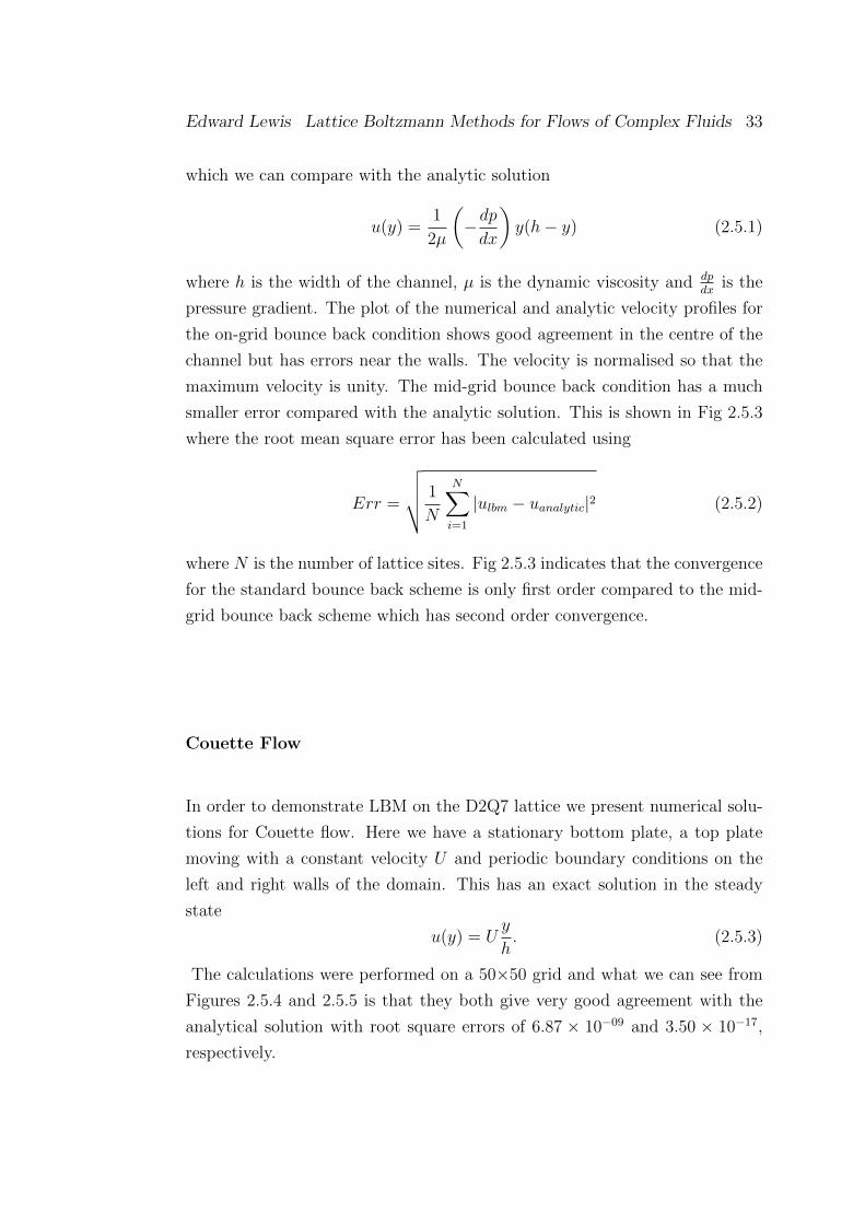
Edward Lewis Lattice Boltzmann Methods for Flows of Complex Fluids 33
which we can compare with the analytic solution
u(y) =1
2µ
(−dpdx
)y(h− y) (2.5.1)
where h is the width of the channel, µ is the dynamic viscosity and dpdx
is the
pressure gradient. The plot of the numerical and analytic velocity profiles for
the on-grid bounce back condition shows good agreement in the centre of the
channel but has errors near the walls. The velocity is normalised so that the
maximum velocity is unity. The mid-grid bounce back condition has a much
smaller error compared with the analytic solution. This is shown in Fig 2.5.3
where the root mean square error has been calculated using
Err =
√√√√ 1
N
N∑i=1
|ulbm − uanalytic|2 (2.5.2)
where N is the number of lattice sites. Fig 2.5.3 indicates that the convergence
for the standard bounce back scheme is only first order compared to the mid-
grid bounce back scheme which has second order convergence.
Couette Flow
In order to demonstrate LBM on the D2Q7 lattice we present numerical solu-
tions for Couette flow. Here we have a stationary bottom plate, a top plate
moving with a constant velocity U and periodic boundary conditions on the
left and right walls of the domain. This has an exact solution in the steady
state
u(y) = Uy
h. (2.5.3)
The calculations were performed on a 50×50 grid and what we can see from
Figures 2.5.4 and 2.5.5 is that they both give very good agreement with the
analytical solution with root square errors of 6.87 × 10−09 and 3.50 × 10⁻¹⁷,
respectively.

34
Figure 2.5.1: Normalised velocity profiles for Poiseuille flow with on-gridbounce back condition with ω = 1.25
Figure 2.5.2: Normalised velocity profiles for Poiseuille flow with mid-gridbounce back condition with ω = 1.25

Edward Lewis Lattice Boltzmann Methods for Flows of Complex Fluids 35
Figure 2.5.3: Comparison between the root mean square error for the mid-gridand on-grid bounce back boundary conditions with ω = 1.25.
Figure 2.5.4: Couette Flow on the D2Q7 lattice, horizontal velocity profile,ω = 1

36
Figure 2.5.5: Couette Flow on the D2Q9 lattice, horizontal velocity profile,ω = 1
2.6 Discussion
In this Chapter we have discussed the implementation of the LBM. What has
been demonstrated is the ease of implementation for a wide variety of flow
scenarios. We started by examining different collision operators used such
as BGK and MRT. The BGK operator is the most widely used do to the
ease of implementation but the MRT has significant advantages due to the
increase in stability of the method. The propagation algorithm used can make
a significant difference to the computational efficiency of the LBM especially
when it is used to solve large problems. The choice of propagation algorithm
is therefore informed by the nature of your computational architecture. Since
the major advantage of using LBM over macroscopic solvers is the ease of
implementing boundary conditions, different boundary conditions have been
discussed and results have been presented demonstrating the advantages of
using the mid-grid bounce back over the on-grid bounce back.

Chapter 3
Lattice Boltzmann Theory
Although the Lattice Boltzmann Method was developed from the Lattice Gas
Cellular Automata, it can be derived independently. Understanding how to
construct the LBM for solving the Navier-Stokes equations using a D2Q9
lattice is important if we want to construct Lattice Boltzmann style solvers
for other equations such as the Fokker-Planck equation which is used in the
modelling of a particle under the influence of drag forces and random forces
as in Brownian motion or for developing Lattice Boltzmann solvers for non-
isothermal flow in which higher order schemes are necessary for thermodynamic
consistency. In this chapter we look at how to derive the Lattice Boltzmann
equation from the continuous Boltzmann equation,the derivation of the equi-
librium distribution function for the Lattice Boltzmann Equation and how the
Lattice Boltzmann Equation is able to reproduce the physics of the Navier-
Stokes equations.
3.1 From the Continuum Boltzmann Equation
to the Lattice Boltzmann Equation
Although as discussed previously, lattice Boltzmann equations were first con-
sidered as empirical extensions of the earlier lattice gas celluar automata
(LGCA), they may be derived systematically by truncating the continuum
Boltzmann equation in velocity space [42, 66, 1]. We consider the continuum
37

38
Boltzmann BGK equation
∂tf + ξ · ∇f = −1
τ(f − f eq) (3.1.1)
with the Maxwell-Boltzmann equilibrium distribution function
f eq =ρ
(2πRT )D/2exp
(−(ξ − u)2
2RT
), (3.1.2)
where the macroscopic variables are determined from the moments of the dis-
tribution function
ρ(x, t) =
∫f(x, ξ, t)dξ, (3.1.3)
ρ(x, t)u(x, t) =
∫ξf(x, ξ, t)dξ, (3.1.4)
ρ(x, t)e(x, t) =
∫(ξ − u)2f(x, ξ, t)dξ, (3.1.5)
where ρ is the fluid density, u is the fluid velocity and e is the internal energy,
the energy contained within the system excluding the kinetic and potential
energy of the system as a whole. Using a Taylor expansion on the equilibrium
equation (3.1.2) up to u2 we obtain
f eq =ρ
(2πRT )D/2exp
(− ξ2
2RT
)(1 +
ξ · uRT
+(ξ · u)2
2(RT )2− u2
2RT
)+O(u3).
(3.1.6)
In order to derive the Navier-Stokes equations, the following moment integral
must be evaluated exactly ∫ξmf eqdξ, (3.1.7)
where 0 ≤ m ≤ 3 for isothermal models [42]. The truncated equilibrium
function has the form
f eq = exp
(− ξ2
2RT
)p(ξ) (3.1.8)

Edward Lewis Lattice Boltzmann Methods for Flows of Complex Fluids 39
where p is a polynomial in ξ and so as He and Luo [42] realised these integrals
may be evaluated as sums using Gauss-Hermitian quadrature formulae,
I =
∫ξm exp
(− ξ2
2RT
)p(ξ)dξ =
∑i=0
Wi exp
(− ξ2
i
2RT
)p(ξi), (3.1.9)
where Wi and ξi are the weights and abscissae of the quadrature respectively.
Since the only values of the distribution function as evaluated at the ab-
scissae need to be evolved in x and t, these values are sufficient to evaluate
the required moments. Thus the continuum Boltzmann BGK equation may
be replaced by the lattice Boltzmann BGK equation, [23]
∂tfi + ξi · ∇fi = −1
τ(fi − f eqi ), for i = 0, . . . , N (3.1.10)
where
fi(x, t) =Wif(x, ξi, t)
exp(− ξ2
2RT
) . (3.1.11)
Accordingly, the macroscopic variables can be computed by quadrature as well
ρ(x, t) =∑i
fi(x, ξi, t), (3.1.12)
ρ(x, t)u(x, t) =∑i
ξifi(x, ξi, t), (3.1.13)
ρ(x, t)e(x, t) =∑i
(ξi − u)2fi(x, ξi, t). (3.1.14)
To derive the previously mentioned D2Q9 model, a Cartesian coordinate
system is used. We set p(ξ) = ξmx ξny and the integral of equation (3.1.9)
becomes
I = (√
2RT )m+n+2ImIn, (3.1.15)
where
Im =
∫ +∞
−∞exp(−z2)zmdz (3.1.16)
where z = ξx/√
2RT or z = ξy/√
2RT . Evaluating Im using Gauss-Hermitian
quadrature the three abscissae zj and the corresponding weights ωj of the

40
quadrature are
z1 = −√
3/2, z2 = 0, z3 =√
3/2, (3.1.17)
ω1 =√π/6, ω2 = 2
√π/3, ω3 =
√π/6, (3.1.18)
then the integral I becomes
I = 2RT
[ω2
2p(0) +4∑i=1
ω1ω2p(ξi) +8∑i=5
ω21p(ξi)
], (3.1.19)
where ξi is the zero velocity vector for i = 0, the vectors of√
3RT (±1, 0) and√3RT (0,±1) for i = 1, . . . , 4 and vectors of
√3RT (±1,±1) for i = 5, . . . , 8.
To obtain the D2Q9 isothermal model we choose√
3RT = c where c is the
ratio the lattice spacing to lattice time step. Thus by comparing equations
(3.1.9) and (3.1.19), we can identify the weights defined in (3.1.9)
Wi = 2πRT exp(ξ2i /2RT )wi, (3.1.20)
where
wi =
4/9, i = 0
1/9, i = 1, . . . , 4
1/36, i = 5, . . . , 8.
(3.1.21)
The discrete equilibrium distribution functions are
f eqi = wiρ
1 +
3(ci · u)
c2+
9(ci · u)2
2c4− 3u2
2c2
. (3.1.22)
In order to fully disretise the lattice Boltzmann equation we must approxi-
mate (3.1.10) in time and space. Integrating (3.1.10) along a characteristic for
a time interval ∆t we obtain
fi(x+ξi∆t, t+∆t)−fi(x, t) = −1
τ
∫ ∆t
0
fi(x+ξis, t+s)−f eq(x+ξis, t+s)ds.
(3.1.23)

Edward Lewis Lattice Boltzmann Methods for Flows of Complex Fluids 41
If we approximate this integral by the trapezium rule, we have
fi(x + ξi∆t, t+ ∆t)− fi(x, t)
= −∆t
2τ(fi(x + ξi∆t, t+ ∆t)− f eqi (x + ξi∆t, t+ ∆t) + fi(x, t)− f eqi (x, t))
(3.1.24)
which unfortunately is implicit. Using a change of variables first suggested by
He et al. [43]
fi(x′, t′) = fi(x
′, t′) +∆t
2τ(fi(x
′, t′)− f eqi (x′, t′)) (3.1.25)
the implicit system can be recast in the explicit form
fi(x + ξi∆t, t+ ∆t)− fi(x, t) = − ∆t
τ + ∆t/2(fi(x, t)− f eqi (x, t)). (3.1.26)
The macroscopic density, momentum and momentum flux are readily recon-
structed from moments of the fi
ρ(x, t) =∑i
fi(x, ξi, t), (3.1.27)
ρ(x, t)u(x, t) =∑i
ξifi(x, ξi, t), (3.1.28)(1 +
∆t
2τ
)Π =
∑i=0
ξiξifi +∆t
2τΠeq. (3.1.29)
It should be noted that this formulation is equivalent to the usual construction
based on a Taylor expansion of the discrete equation where second order accu-
racy may be achieved with what looks like only a first order approximation to
(3.1.10), by replacing the relaxation time τ with τ + ∆t/2 [17]. The variables
often denoted fi appearing in the discrete system are actually the fi in our
notation, so that the non-equilibrium momentum flux Π(1) in the fully discrete
system (3.1.26) is given by
Π(1) =Π−Πeq
1 + ∆t/(2τ), (3.1.30)
rather than by Π−Πeq as in the continuous system.

42
3.2 Derivation of the Equilibrium Distribution
Function
There are two methods by which the local equilibria for the Lattice Boltzmann
Equation can be constructed. The bottom-up method obtains the equilibrium
from the Maxwell-Boltzmann equilibrium distribution. The top-down method
constructs the equilibrium so that the required macroscopic properties can be
reproduced.
Equilibrium from the Maxwell-Boltzmann equilibrium distribution
The equilibrium distribution f eq is given by
f eq =ρ
(2πθ)D/2e−(v−u)2/2θ (3.2.1)
where θ = c2s = kT/m is the scaled temperature, k is the Boltzmann constant,
T is the fluid temperature, v is the microscopic velocity, u is the mean fluid
velocity, D is the space dimension, and m is the mass of the particle. The
parameter cs is the speed of sound in a gas close to equilibrium described by
f eq.
When |v − u| √θ, the equilibrium distribution can be expanded and
approximated by
f eq =ρ
(2πθ)D/2exp
(−v
2
2θ
)[1 +
v · uθ
+(v · u)2
2θ2− u2
2θ
](3.2.2)
For a microscopic quantity ψ(v), the associated macroscopic quantity Ψ is
calculated by
Ψ =
∫ψ(v)f eqdv (3.2.3)
Let v =√
2θc, where c is a rescaled thermal velocity; the macroscopic
velocity u can be similarly rescaled to√
2θu. Equations (3.2.2) and (3.2.3)
can thus be combined to give
Ψ =
∫e−c
2
ψ(c)
√2θρ
(2πθ)D/2[1 + 2(c · u) + (c · u)2 − u2
]dc (3.2.4)

Edward Lewis Lattice Boltzmann Methods for Flows of Complex Fluids 43
Using Gaussian-Hermite quadrature to approximate the integral yields
Ψ '∑
ψ(ci)
√2θ
(2πθ)D/2w(ci)
[1 + 2(c · u) + (c · u)2 − u2
]dc (3.2.5)
Let
wi =
√2θρ
(2πθ)D/2w(ci) (3.2.6)
and
f eqi = wiρ[1 + 2(c · u) + (c · u)2 − u2
]. (3.2.7)
The value of w(ci) can be obtained from Gauss-Hermite quadrature. Equa-
tion (3.2.7) is the equilibrium particle distribution function in the discrete
regime and wi is called the weight factor for speed vector vi. Equation (3.2.7)
can also be written in the form
f eqi = wiρ
[1 +
(ci.u)
θ+
(ci.u)2
2θ2− u2
2θ
]. (3.2.8)
Constructing the equilibrium from the required macroscopic prop-
erties
The second way of constructing the equilibrium distribution is by starting
from the macroscopic properties and solving the linear system to recover the
coefficients of the equilibrium function. Here we give as an example the D2Q9
model as given by Reis [84].
The general form of the equilibrium distribution function can be written
up to O(u2) [15]:
f eqi = ρwi(A+Bci · u + Cu2 +D(ci · u)2
)(3.2.9)
where A,B,C and D are constants. The weights wi, i = 0, . . . , 8 are chosen
to be positive to ensure positive mass density and so that the lattice velocity
moments coincide with those of the Maxwell distribution up to fourth order

44
i.e.
8∑i=0
wi = 1, (3.2.10)
8∑i=0
wiciα = 0, (3.2.11)
8∑i=0
wiciαciβ = θδαβ, (3.2.12)
8∑i=0
wiciαciβciγ = 0, (3.2.13)
8∑i=0
wiciαciβciγciδ = θ2(δαβδγδ + δαγδβδ + δαδδγβ), (3.2.14)
where δαβ is the Kronecker delta function and ciα denotes the α component of
the ith lattice velocity.
Using mass conservation (1.3.6)
ρ = ρ(A+ Cu2 +Duαuβθδαβ) (3.2.15)
so we see that at 0th order
A = 1, (3.2.16)
and at order O(u2):
C +Dθ = 0. (3.2.17)
Now using momentum conservation (1.3.7)
B =1
θ. (3.2.18)
Defining the momentum flux tensor, Παβ, to be the second moment of the
equilibrium function we find that
Παβ =8∑i=0
f eqi ciαciβ, (3.2.19)
= p0δαβ + ρuαuβ (3.2.20)

Edward Lewis Lattice Boltzmann Methods for Flows of Complex Fluids 45
where p0 = θρ and we have set (at order u2)
Cθ + 3Dθ2 = 1, (3.2.21)
and (at order O(uαuβ))
2Dθ2 = 1. (3.2.22)
A little algebra reveals that
B = 3, (3.2.23)
C = −3
2, (3.2.24)
D =9
2, (3.2.25)
θ =1
3(3.2.26)
and the weights are
wi =
49
i = 0
19
i = 2, 4, 6, 8
136
i = 1, 3, 5, 7.
(3.2.27)
Therefore, the D2Q9 equilibrium function is given by
f eqi = ρwi
(1 + 3ci · u +
9
2(ci · u)2 − 3
2u2
)(3.2.28)
with pressure p0 defined by
p0 =ρ
3. (3.2.29)
Note that the pressure satisfies an ideal equation of state and the factor 1/3
is the speed of sound squared, i.e. c2s = 1/3.
A similar analysis can be performed for the D2Q7 lattice. The equilibrium
for the moving particles have the general form
f eqi = d+ρ
3c2ci · u + ρ
2
3c4(ci · u)2 + γu2 (3.2.30)
and the equilibrium distribution for the rest particles has the form
f eq0 = d0 + γ0u2 (3.2.31)

46
where d, d0, γ and γ0 are coefficients to be determined and c is the length of a
lattice vector. Examining the mass conservation law we derive the following
constraints
ρ = d0 + 6d, (3.2.32)
0 = γ0 + ρ2
c2+ 6γ (3.2.33)
and the momentum flux tensor can be expressed as
Πij =∑α
(cα)i(cα)jfeqα = 3c2dδij + ρuiuj +
(ρ2
+ 3c2γ)
u2δij, (3.2.34)
which satisfies the requirement of Galilean invariance. It can immediately be
seen that the velocity dependence of the pressure is eliminated by setting
γ = − ρ
6c2. (3.2.35)
We can then solve equation (3.2.33) to find γ0 = −ρ/c2. The choice of d0 is
rather arbitrary but is commonly chosen so that d0 = ρ0/7 where ρ0 is the
total number of particles divided by the total number of lattice sites. Since d0
is a constant d is seen to be linearly dependent on the total particle density ρ
with the pressure related to the total particle density having the form for an
isothermal ideal gas,
p = c2sρ. (3.2.36)
3.3 Relation Between the Lattice Boltzmann
Method and Navier-Stokes
In this chapter we show why LBM can be used to simulate fluid dynamics
by showing that one can, by use of multiscale analysis (commonly referred
to as the Chapman-Enskog procedure), derive the Navier-Stokes equations.
Applying the BGK approximation to the collision operator we define the LBGK
equation to be
fi(x + ci, t+ 1)− fi(x, t) = −1
τ
(fi − f (0)
i
)(3.3.1)

Edward Lewis Lattice Boltzmann Methods for Flows of Complex Fluids 47
Expanding fi(x + ci, t + 1) about the point (x, t) and defining fi = fi(x, t)
gives
∂tfi+ciα∂αfi+1
2(∂ttfi + 2ciα∂t∂αfi + ciαciβ∂α∂βfi) = −1
τ
(fi − f (0)
i
)(3.3.2)
Now separate space and time scales as
x =1
εx1, t =
1
εt1 +
1
ε2t2 (3.3.3)
so that ∂t = ε∂t1 + ε2∂t2 , ∂x = ε∂x1 This means that the second-order partial
derivatives are
∂tt = ε2∂t1t1 + 2ε3∂t1∂t2 + ε4∂t2t2 (3.3.4)
∂αα = ε2∂α1α1 (3.3.5)
∂t∂α = ε2∂t1α1 + ε3∂t2α1 (3.3.6)
Using these with (3.3.2) gives
ε∂t1fi + ε2∂t2fi + ciα1ε∂α1fi +1
2
[ε2∂t1t1fi + 2ε3∂t1t2fi + ε4∂t2t2fi
+2ciα1
(ε2∂t1∂α1fi + ε3∂t2∂α1fi
)+ ciα1ciβ1ε
2∂α1∂β1fi]
= −1
τ
(fi − f (0)
i
)(3.3.7)
Now we say that the particle distribution function departs slightly from
the local equilibrium state and write
fi = f(0)i + εf
(1)i + ε2f
(2)i + . . . (3.3.8)
and then substitute (3.3.8) into (3.3.7) and compare coefficients of ε. At first
order in ε we have
∂t1f(0)i + ciα∂αf
(0)i = −1
τf
(1)i (3.3.9)
Using mass conservation (taking moments) of (3.3.9) we obtain
∂t1ρ+ ∂αρuα = 0 (3.3.10)

48
and momentum conservation yields
∂t1ρuα + ∂βΠαβ = 0. (3.3.11)
The O(ε2) terms give
∂t1f(1)i + ∂t2f
(0)i + ciα1∂α1f
(1)i +
1
2∂t1t1f
(0)i
+ciα1∂t1∂α1f(0)i +
1
2ciα1ciβ1∂α1∂β1f
(0)i = −1
τf
(2)i (3.3.12)
and taking zeroth order moments gives
∂t2ρ+1
2∂t1t1ρ+ ∂t1∂αρuα +
1
2∂α∂βΠαβ = 0. (3.3.13)
Differentiating (3.3.10) with respect to t1 and (3.3.11) with respect to α
yields
∂t1t1ρ = −∂t1∂αρuα,
∂α∂t1ρuα + ∂α∂βΠαβ = 0,
⇒ ∂t1t1ρ = −∂t1∂αρuα = ∂α∂βΠαβ (3.3.14)
and substituting this into (3.3.13) shows that
∂t2ρ = 0, (3.3.15)
which with (3.3.10) yields the continuity equation:
∂tρ+∇ · ρu = 0. (3.3.16)
Next taking first order moments of (3.3.12) we find
∂t2ρuα + ∂βQαβ +1
2∂t1t1ρuα︸ ︷︷ ︸
=− 12∂t1∂βΠαβ
+∂t1∂βΠαβ +1
2∂β∂γPαβγ = 0 (3.3.17)
⇒ ∂t2ρuα + ∂βQαβ +1
2∂t1∂βΠαβ +
1
2∂β∂γPαβγ = 0, (3.3.18)

Edward Lewis Lattice Boltzmann Methods for Flows of Complex Fluids 49
where Pαβγ =∑
i f(0)i ciαciβciγ and Qαβ =
∑i f
(1)i ciαciβ.
For the D2Q9 lattice the momentum flux tensor which gives rise to the
Newtonian stress tensor, is
Παβ = p0δαβ + ρuαuβ, (3.3.19)
where pressure p0 = ρ/3. Differentiating the momentum flux tensor with first
with respect to time and space yields
∂t1Παβ = ∂t1
(ρ3δαβ + ρuαuβ
)(3.3.20)
= ∂t1ρ
3δαβ + ∂t1(ρuαuβ) (3.3.21)
= −1
3∂αρuαδαβ + ∂t1(ρuαuβ) (3.3.22)
and
∂t1∂βΠαβ == −1
3∂α∂βρuαδαβ + ∂t1∂β(ρuαuβ) (3.3.23)
which up to second order in u (low Mach number approximation) gives,
∂t1∂βΠαβ = −1
3∂α∂βρuβ (3.3.24)
and
∂β∂γPαβγ =1
3(∂β∂βρuα + 2∂α∂βρuβ). (3.3.25)
To find Qαβ we take the second moment of equation (3.3.9)
∂t1Παβ + ∂γPαβγ = −1
τQαβ
so that
Qαβ = −τ (∂t1Παβ + ∂γPαβγ) . (3.3.26)
The substitution of the above into (3.3.18) gives
∂t2ρuα +
(1
2− τf
)(∂t1∂βΠαβ + ∂β∂γPαβγ) = 0. (3.3.27)

50
This can be written as
∂t2ρu = ν(∇2ρu +∇∇ · ρu), (3.3.28)
where
ν =1
3
(τf −
1
2
), (3.3.29)
is the kinematic viscosity and we note that 0 < 1τf< 2.
Finally, summing equations (3.3.11) and (3.3.28), assuming incompressibil-
ity we arrive at the Navier-Stokes equations for incompressible flow:
∂tu + u · ∇u = −1
ρ∇p0 + ν∇2u, (3.3.30)
∇ · u = 0. (3.3.31)
3.4 Discussion
In Chapter 3 the derivation of the equilibrium distribution function is given in
two ways. Firstly it is given as a discretised version of the Maxwell-Boltzmann
equilibrium distribution using Gauss-Hermite quadrature and secondly it is
constructed from the macroscopic properties required and using them to solve
the linear system to recover the coefficients of the equilibrium function. Also
in Chapter 3 is the relation between the LBM and Navier-Stokes equations
which is given by the Chapman-Enskog multiscale procedure. Chapter 3 is
vital when looking for ways to adapt the LBM to solve other problems such
as the Fokker-Planck equation as will be shown in Chapter 7.

Chapter 4
Multiphase fluid flows
Multiphase flows are of great importance to industry and applied science as
they include processes such as boiling fluids, liquid metal melting and so-
lidification, and even food manufacturing processes such as the creation of
mayonnaise.
The numerical simulation of multiphase flows is challenging because in ad-
dition to the usual difficulties associated with tracking single phase motion,
it also requires the calculation of the interface between the two fluids which
changes dynamically in time. Existing methods that deal with moving inter-
faces generally fall into two distinct categories which are front tracking and
front capturing.
In front tracking methods, markers are attached to the moving interface
and their dynamics are explicitly designed so that they follow the interface
evolution. As long as the interface remains sufficiently smooth, the interface
can be tracked fairly accurately. If the interface breaks up and reconnects, front
tracking suffers from the similar difficulty of Lagrangian methods, namely ill-
conditioning and singularities due to markers coming too close to each other.
The main developers of this approach are Glimm and collaborators [34, 20, 35,
33].
Front capturing methods solve this problem by using an Eulerian approach
and defining a data structure throughout the whole computational domain.
The interface is located by examining where the discontinuities take place.
These methods avoid the problems associated with large distortions of the in-
terface but they suffer from severe numerical diffusion effects which tend to
51

52
smear out the interface in the course of the computation. Front capturing
methods are actually the oldest approach to computing multifluid and mul-
tiphase flows. The marker and cell (MAC) method, uses marker particles to
identify each fluid and was developed by Harlow and Welch [39] in 1965. The
volume of fluid (VOF) method which was first described by Noh and Wood-
ward in 1976 [73] and is based on earlier MAC methods. A modern formulation
of VOF is used in a number of computer codes, such as FLOW-3D, ANSYS
Fluent and STAR-CCM. A review of the VOF method can be found in Scar-
dovelli and Zaleski [90].
From a review of the literature, we shall discuss four different formulations
of LBM for immiscible multiphase flows, namely;
• Chromodynamic models (see [36]);
• Pseudo-potential models (see [95]);
• Free-energy models (see [101]);
• Mean-field models (see [43]).
There seems to be no general consensus yet on which one of these methods
should be recommended as the best LBE solution for multiphase problems. In
fact, all of them are still affected by a certain degree of inevitable empiricism
due to the fact that, even in the continuum, a fully fledged kinetic theory of
complex fluid flow is still missing. It seems that all of the LBE models belong
to a wide family of diffuse-interface models where the interface is located over
several lattice points, the width of which is greatly influenced by the choice of
multiphase model.
4.1 Surface Tension
Before we begin a discussion of various LBE models we consider some basic
ideas of the physics of multiphase flows. The key to the physics of multiphase
flows is the notion of surface tension. From a macroscopic perspective, surface
tension (σ) is defined as the reversible work per unit surface needed to increase

Edward Lewis Lattice Boltzmann Methods for Flows of Complex Fluids 53
the area A of surface Σ by an amount ∆A:
∆W = σ∆A. (4.1.1)
If we consider a spherical liquid droplet of radius R at a pressure Pl, im-
mersed in its vapour at a pressure Pv > Pl. The question is how much work is
spent on the vapour-liquid system to expand the radius of the liquid droplet
from R to R+∆R (condensation). This work is given by ∆W = (Pv−Pl)∆V ,
where ∆V = 4πR2∆R is the volume change of the droplet. This is the energy
supply from the exterior needed to win the action of surface tension, whose
‘task’ is to withstand the growth of the liquid surface. Mathematically we
have:
(Pv − Pl)∆V = σ∆A. (4.1.2)
Using the equation for the surface area of a sphere (A = 4πR2), we obtain
the Laplace relation:
∆P =2σ
R. (4.1.3)
From a microscopic perspective, surface tension is related to intermolecu-
lar interactions. Imagining the same liquid droplet as before, we consider a
molecule sitting right on the droplet interface. Since the liquid is more dense
than the vapour, this boundary molecule interacts with more liquid molecules
than vapour molecules and since the intermolecular potential is attractive (van
der Waals forces, hydrogen bonding etc.), the net result is that the boundary
molecule naturally tends to be pulled back into the liquid region. This is in
contrast to the situation of an internal molecule which, being surrounded by
an equal number of molecules in all directions, does not experience any net
force.
The conclusion we reach is that a surface molecule has an excess of energy
with respect to an internal one, the difference representing the work needed
to extract the internal molecule and ‘peel it off’ the surface. The same energy
must be supplied to push a vapour molecule inside the liquid droplet, so that
surface growth involves an energy toll. This implies that surface tension is a
decreasing function of temperature and vanishes at the critical liquid-vapour
point, where the two phases become virtually indistinguishable.

54
4.2 Chromodynamic models
The first multiphase LBE model was introduced by Gunstensen et al. [36],
based upon the two component lattice gas model developed by Rothman and
Keller [88].
In these models we have two particle distributions fiR and fiB, one for each
fluid. It is common to call these fluids Red (R) and Blue (B). Each phase
obeys its own LBGK equation:
∆ifis = −ωs(fis − f eqis ) + Sis, i = 1, . . . , b s = R, B. (4.2.1)
The source term Sis represents the mesoscopic interaction between the two
phases and it is therefore the term responsible for describing phase separation
via surface tension effects. For example, Reis and Phillips [85] handle the
source term by a second collision operator.
The central quantities are the colour gradient F(x) and the colour flux
K(x) defined as follows:
F(x) =∑i
ci[ρr(x + ci)− ρb(x + ci)] (4.2.2)
and
K(x) =∑i
(fiR − fiB)ci. (4.2.3)
Reis and Phillips [85] choose the source term so that the correct form of
the continuum equations are recovered. The source term adds mass to popu-
lations moving in the direction normal to the red-blue interface and removes
mass parallel to the interface. Since this term does not conserve colour densi-
ties separately an additional step is needed to promote phase segregation and
maintain surfaces between fluids. Succi [100] notes ‘that such a type of ‘smell
and go’ dynamics is commonplace in many other sectors of complex fluid dy-
namics, including polar fluids and biological flows.’ Reis and Phillips suggest
minimising the ‘colour energy’ Q = K · F to break the colour symmetry and
cause the red and blue particles to move in preferential directions and maintain
surfaces. This however would involve variational minimisation at every single
lattice site where there is a mixture of fluids and is computationally expensive.

Edward Lewis Lattice Boltzmann Methods for Flows of Complex Fluids 55
Lischuk et al. [62] and Halliday et al. [38] proposed using a continuum surface
force to model interfacial tension and promote segregation using the algorithm
by D’Ortona et al. [27] which gives a non-zero boundary thickness between the
fluids and reduces non-physical effects such as pinning of drops to the lattice,
spatial anisotropy in interfacial tension and spurious microcurrents.
Chromodynamic models have some positive and some negative features.
With refinement it is able to handle many different phases. For example,
DL MESO [93] is capable of computing up to six different phases and the
method is able to model phases with a high density ratio (O(1000)). It is
important to note that with chromodynamic approaches, the diffusive interface
can be kept very sharp, of the order of one or two lattice sites.
The “coloured fluid” model has some issues, it is more complicated and
computationally expensive to implement than the pseudo-potential model and
the method is only valid for isothermal flows.
4.3 The pseudo-potential approach
The chromodynamic approach of Gunstensen [36] is based on a significant
abstraction of the physical reality. The ‘colour force’ is nothing but the logical
statement that molecules sitting at the interface between, say, dense and light
fluids, experience a net force driven by the different values of the average
intermolecular distance in the two fluids. It is therefore natural to look for
more physically-oriented representations, in which these forces are directly
encoded as the result of pairwise molecular interactions.
[95] model interactions between multiple phases and components by calcu-
lating pairwise interaction potentials. These potentials use an ‘effective mass’
for each component, ψa, which is a function of density and is most frequently
defined as
ψa(x) = ρa0
[1− exp
(−ρ
a(x)
ρa0
)](4.3.1)
where ρa is the local density of component a and ρa0 is the reference density
for the same component.
Defining gab as the interaction coefficient between components a and b, the
overall force on component a due to interactions with other components is

56
defined as
Fa = −ψa(x)∑b
gab∑i
wiψb(x + ci)ci (4.3.2)
There are a few different ways of implementing this force such as adding τfF/ρ
to the velocity of the fluid when calculating the equilibrium distribution func-
tion f eqi , or adding a forcing term to the collisional distribution function which
is favoured by Guo et al. [37].
The Shan-Chen model is able to simulate many phase separation and in-
terface phenomena and it is quick to run and code, although it struggles to
simulate phases with density ratios bigger than O(100).
The main drawback of the Shan-Chen model is the lack of thermodynamics
as first pointed out by Swift et al. [101]. The thermodynamic inconsistency
of the Shan-Chen model can be better explained by examining the pressure
tensor. By expanding equation (4.3.2) about x and recognising that
∇ ·P = ∇(ρRT )− F (4.3.3)
must be satisfied at equilibrium we recover
P =
[ρRT +
gRT
2ψ2 +
g(RT )2
2(ψ∇2ψ +
1
2|∇ψ|2)
]I− g(RT )2
2∇ψ∇ψ.
(4.3.4)
This pressure tensor implies that the Shan-Chen model has the two basic
properties of non-ideal gases:
(i) An equation of state of the form
p0 = ρRT +gRT
2ψ(ρ)2, (4.3.5)
(ii) and the surface tension
σ =gRT
2∞infty−∞ |∇ψ|2dz. (4.3.6)
However, to be consistent with the equation of state in thermodynamic theory,
we must have
ψ =
√2(p0 − ρRT )
gRT(4.3.7)

Edward Lewis Lattice Boltzmann Methods for Flows of Complex Fluids 57
On the other hand, to be consistent with the thermodynamic definition of the
surface tension given by Rowlinson and Widom [89],
σRowlinson ∝∫ ∞−∞|∇ρ|2dz (4.3.8)
we must have
ψ ∝ ρ. (4.3.9)
Since equations (4.3.7) and (4.3.9) cannot be satisfied simultaneously, the
Shan-Chen model is thermodynamically inconsistent. The assumption that
causes this inconsistency is that a molecule only interacts with its nearest
neighbours. The idea of only using nearest neighbour interactions originates
from the celebrated Ising model but may not be appropriate for describing
molecular interactions in dense fluids. Nearest neighbour interactions only
have one characteristic length (the lattice size) and therefore is not sufficient to
describe the Lennard-Jones potential where both short range repulsion (Pauli
repulsion at short ranges due to overlapping electron orbitals) and long range
attraction (van der Waals forces) are important.
Figure 4.3.1: Lennard Jones Potential

58
4.4 The free energy approach
A step forward in the direction of thermodynamic consistency was taken by
Swift et al. [101]. These authors introduce the equilibrium pressure tensor for
a non-ideal fluid directly into an extended form of the collision operator. The
idea is that, by doing so, the fluid is instructed to reach the right thermody-
namic equilibrium directly under the effect of the correct equation of state.
The method of Swift et al. [101] builds on the van der Waals formulation of
a two component isothermal fluid. The basic object of the theory is the free
energy density functional Ψ, (free energy per unit volume) defined as
Ψ[ρ] =
∫1
2k[(∇ρ)2 + ψ(ρ)
]dV, (4.4.1)
where the first term is the energy penalty paid to build density gradients, and
the second term is the bulk free energy where ψ is the free-energy density. The
non-local pressure relates to Ψ through the following expression:
P = ρdΨ
dρ−Ψ = P0 − kρ∇2ρ2 − 1
2k|∇ρ|2, (4.4.2)
where
P0 = ρΨ′ −Ψ (4.4.3)
is the equation of state of the fluid (prime stands for derivative with respect
to density). The full pressure tensor in a non-uniform fluid includes an off-
diagonal component
Pab = Pδab + k∂aρ∂bρ, (4.4.4)
where the second term is related to interfacial surface tension effects.
An important question is how do we encode this pressure tensor in the
equilibrium distribution?
The recipe is to add (weakly) non-local terms to the discrete equilibria.
In particular, for a seven state FHP lattice, Swift et al. [101] propose the
following expression:
f eqi = A+Bciαuα + Cu2 +Dciαciβuαuβ + Fαciα +Gabciαciβ, (4.4.5)
f eq0 = A0 + C0u2 (4.4.6)

Edward Lewis Lattice Boltzmann Methods for Flows of Complex Fluids 59
The Lagrangian parameters A,B,C,D, Fα, Gαβ are prescribed by the usual
conservation of mass, momentum and momentum flux tensor constraints, with
Pαβ given by (4.4.4). These relations are sufficient to compute the parame-
ters as a function ρ and its spatial derivatives, thus solving the problem of
identifying a proper free energy for the multiphase LB system.
Swift et al. [101] demonstrate their model with 2D simulations based on
the van der Waals fluid energy density ΨV dW = ρT ln ρ/(1 − ρb) − aρ2. Like
their predecessors, they test their scheme against Laplace’s law:
Pin − Pout =σ
R, (4.4.7)
where ‘in/out’ refer to inner/outer pressure of a bubble of radius R. Another
test refers to the dispersion relation of capillary waves. They also compute
the coexistence curve between the two phases for several values of the (static)
fluid temperature, reporting excellent agreement with thermodynamic theory.
The main drawback to using a free energy model is that they suffer from
a lack of Galilean invariance in the viscous term when one derives the Navier-
Stokes equations. This introduces spurious currents in the interface whenever
there is a density gradient. There is one case where the model of Swift et al.
[101] works consistently which is for a binary fluid where each fluid is an ideal
gas.
4.5 Mean field model
He et al. [43] proposed an LBM multiphase model based on mean field theory
and Enskog’s model for dense fluids. It was demonstrated later that the mean
field model can be derived from the BBGKY theory with appropriate approx-
imations [41]. BBGKY theory (Bogoliubov-Born-Green-Kirkwood-Yvon the-
ory) is a set of equations describing the dynamics of a system of a large number
of interacting particles. The equation for an n particle distribution function
in the BBGKY theory includes the (n+ 1) particle distribution function thus
forming a coupled chain of equations. To close this system, approximations
have to be introduced The key to the mean field model is to use mean field
theory to describe the long range attraction among molecules, while using the

60
Enskog theory for dense fluids to account for short range repulsion. According
to Chen et al. [18] we see that the mean field model not only recovers the
correct mass, momentum and energy equations, it also contains the correct
thermodynamics.
Historically, kinetic theory was first developed for studying ideal gas trans-
port. To extend its application to phase transitions and multiphase flows, one
must incorporate molecular interactions which become increasingly important
in most fluids as the density increases.
The mean field LBM multiphase model is derived from kinetic theory with
the intermolecular potential incorporated intrinsically. From this perspective,
it inherits the fundamental feature of the inter-particle potential model. At
the same time, the mean field theory guarantees thermodynamic consistency.
In the theory of the BBGKY hierachy, the evolution equation for the single-
particle distribution, f(ξ1, r1), is:
∂tf + ξ1 · ∇r1f + F · ∇ξ1f =
∫ ∫∂f (2)
∂ξ1
· ∇r1V (r12)dξ2dr2 (4.5.1)
where F is the external force, ξ1 and ξ2 are microscopic velocities, f (2)(ξ1, r1, ξ2, r2)
is the two-particle distribution function, and V (r12) is the pair-wise intermolec-
ular potential between particle 1 and particle 2. In the BBGKY hierarchy of
equations, the time evolution of n-particle distribution depends on the (n+1)st
particle distribution. Approximations have to be introduced to close this for-
mulation.
He and Doolen [41] perform a simple closure at the level of the two-particle
distribution. They begin by dividing the space integral domain of the right
hand side of equation (4.5.1) into two parts: D1 : |r2 − r1| < d and D2 :
|r2 − r1| ≥ d:
∫ ∫∂f (2)
∂ξ1
· ∇r1V (r12)dξ2dr2
=
∫ ∫D1
∂f (2)
∂ξ1
· ∇r1V (r12)dξ2dr2︸ ︷︷ ︸J1
+
∫ ∫D2
∂f (2)
∂ξ1
· ∇r1V (r12)dξ2dr2︸ ︷︷ ︸J2
(4.5.2)

Edward Lewis Lattice Boltzmann Methods for Flows of Complex Fluids 61
where d is the effective diameter of molecules. It is known that many inter-
molecular potentials can be approximated by the Lennard-Jones potential (see
Fig 4.3.1), which possesses a short-range strong repulsive core and a long range
weak attractive tail. Here the first integral, J1, describes the strong repul-
sive force which dominates short range molecular interaction and the second
integral, J , describes the weak attractive force which dominates long range
molecular interaction.
The short range behaviour is essentially a collision process where the rate
of change of the single particle distribution in this process, J1, can be well
modelled by Enskog’s theory for dense fluids [13]:
J1 =
∫D1
∫∂f (2)
∂ξ1
· ∇r1V (r12)dξ2dr2
= χΩ0 − bρχf eq
(ξ − u) ·[∇ log(ρ2χT ) +
3
5
(C2 − 5
2
)∇ log T
]+
2
5
[2CC : ∇u +
(C2 − 5
2
)∇ · u
](4.5.3)
where Ω0 is the ordinary collision term which neglects particle size; C =
(ξ − u)/√
2RT and C is its magnitude; “:” represents the scalar product of
two tensors; ρ,u, and T are the macroscopic density, velocity and temperature,
respectively, f eq is the Maxwell equilibrium distribution function:
f eq =ρ
(2πRT )3/2exp
[−(ξ − u)2
2RT
](4.5.4)
χ is the density dependent collision probability,
χ = 1 +5
8bρ+ 0.2869(bρ)2 + 0.1103(bρ)3 + 0.0386(bρ)4 + . . . (4.5.5)
where b = 2πd3/3m, with d being the diameter and m the molecular mass.
Notice that the corresponding χ for the van der Waals’ equation of state is:
χ =1
1− bρ(4.5.6)
which only agrees with Eq. (4.5.5) to zeroth order.
62
The rate of change of the single particle distribution due to long range
molecular interaction is neglected in Enskog’s original work. It can be very
important in real fluids. Modern physics has shown that, for most liquids, the
radial distribution function is approximately unity beyond a distance of one
molecular diameter [83]. This implies that f (2)(ξ1, r1, ξ2, r2) ≈ f(ξ1, r1)f(ξ2, r2)
in D2. This approximation leads to:
J2 =
∫D2
∫∂f (2)
∂ξ1
· ∇r1V (r12)dξ2dr2 = ∇∫
D2
ρ(r2)V (r12)dr2
· ∇ξ1f.
(4.5.7)
The term in the bracket is exactly the mean field approximation for the
intermolecular potential [89]:
Vm =
∫D2
ρ(r2)V (r12)dr2 (4.5.8)
Its gradient gives the average force acting on a molecule by the surrounding
molecules. Assuming the density is a slowly varying variable, we can expand
the density in a Taylor series:
ρ(r2) = ρ(r1) + r21 · ∇ρ+1
2r21r21 : ∇∇ρ+ . . . (4.5.9)
where r21 = r2 − r1. Substituting Eq. (4.5.9) into Eq. (4.5.8), we have:
Vm ' −2aρ− κ∇2ρ (4.5.10)
where the coefficients a and κ are defined in terms of the intermolecular po-
tential by:
a = −1
2
∫r>d
V (r)dr, κ = −1
6
∫r>d
r2V (r)dr
a and κ are usually assumed to be constant. The integral, J2, subsequently
becomes:
J2 = ∇Vm · ∇ξ1f. (4.5.11)
This form of J2 suggests that the average long range intermolecular po-
tential acts on a molecule in exactly the same way as an external potential. In
other words, the long range molecular interaction can be modelled as a local
point force. It should be mentioned that the above derivations depend on the

Edward Lewis Lattice Boltzmann Methods for Flows of Complex Fluids 63
assumption that density varies slowly. This obviously is a source of at least
some of the issues when modelling binary fluids with a large density ratio.
Combining Enksog’s theory for dense fluids and mean field theory for the
intermolecular potential, one obtains the following kinetic equation to describe
the flow of dense fluids [43]:
∂tf + ξ · ∇f + F · ∇ξf = J1 +∇Vm · ∇ξf (4.5.12)
where the subscripts have been dropped for simplicity. The macroscopic fluid
density, ρ, velocity, u, and the temperature, T , are calculated as the velocity
moments of the distribution functions:
ρ =
∫fdξ (4.5.13)
ρu =
∫ξfdξ (4.5.14)
3ρRT
2=
∫(ξ − u)2
2fdξ. (4.5.15)
It is important to note that J1, in general, cannot be expressed as product
of a single force and velocity gradient of the distribution function. As a result,
the molecular interaction as a whole also cannot be modelled by a single force
term, as in the Shan-Chen model.
Any numerical approach can be used to solve the kinetic equation, but ob-
viously we will focus on a discrete numerical lattice Boltzmann based scheme.
The lattice restricts the molecule movements and this constraint can cause
issues with non-isothermal flows. To study thermodynamics in which temper-
ature variation exists, the theory must be extended. In the study performed by
He and Doolen [41], is an expansion approach for small temperature variations.
Most LBM models neglect terms of order M3 (M is the Mach number).
This cut off error does not hamper LBM applications to nearly incompressible
flows. [41] assume further that the variation of the absolute temperature is
small in the domain of interest.
To facilitate the discussion, they introduce:
T = T0(1 + θ) (4.5.16)

64
where T0 is the average temperature of a system and θ is the normalized tem-
perature variation. With the assumptions of small temperature variations and
small Mach numbers, the equilibrium density distribution can be approximated
by:
f eq =ρ
(2πRT0)3/2exp
[− ξ2
2RT0
] [1 +
(ξ2
2RT0
− 3
2
)θ
+ξ · uRT0
+(ξ · u)2
2(RT0)2− u2
2RT0
]. (4.5.17)
Using this equilibrium distribution, the next task is to select a discrete
velocity set, or quadrature, that replaces the moment integrals in calculating
macroscopic variables. It should be noted that the traditional D2Q7, D2Q9,
D3Q15, D3Q19 and D3Q27 lattices are inadequate for this type of thermal
model as a second-order time integration scheme is necessary, suitable quadra-
tures with higher accuracy can be found in [77].
Nevertheless, once a sufficiently accurate quadrature is chosen (ca, a =
1, 2, . . . , N), we can define the discrete distribution function as:
fa(r, t) = waf(r, ca, t) (4.5.18)
where wa are the corresponding weight coefficients. If we use the BGK model
with a single relaxation time approximation for the ordinary collision term we
assume:
∇ξf ≈ −(ξ − u)
RTf eq (4.5.19)
the evolution equation for the discrete distribution function, fa, becomes:
fa(r + caδt)− fa(r, δt) = −χ(fa − f eqa )
τf + 0.5+
τfτf + 0.5
Ωafeqδt (4.5.20)
where δt is the time step and τf is the relaxation parameter;
Ωa =(ca − u) · (F−∇Vm)
RT− bρχ
(ca − u) ·
[∇ log(ρ2χT ) +
3
5
(C2a −
5
2
)∇ log T
]+
2
5
[2CaCa : ∇u +
(C2a −
5
2
)∇ · u
](4.5.21)

Edward Lewis Lattice Boltzmann Methods for Flows of Complex Fluids 65
Ca = (ca − u)/√
2RT and Ca is its magnitude. The equilibrium distributions
have the following forms:
f eqa = wa
[1 +
(ξ2
2RT0
− 3
2
)θ +
ξ · uRT0
+(ξ · u)2
2(RT0)2− u2
2RT0
](4.5.22)
Note that at least a second order time integration is necessary for LBM
multiphase models [43]. Otherwise, non-physical properties such as spurious
currents arise in simulations.
The macroscopic variables can be calculated using:
ρ =∑a
fa (4.5.23)
ρu =∑a
faca +δt2
[ρF− ρ∇Vm −∇(bρ2χRT )] (4.5.24)
3ρRT
2=
3ρRT0(1 + θ)
2=∑a
fa(ca − u)2
2(4.5.25)
The viscosity and thermal conductivity of the above model have the following
forms:
µ = τfρRT0δt
(1
χ+
2
5bρ
)(4.5.26)
λ =5
2τfρR
2T0δt
(1
χ+
3
5bρ
)(4.5.27)
According to the authors the implementation of the model is straightfor-
ward. Besides the need for higher order velocity lattices, the only compli-
cation compared to the ideal gas LBM model is the calculation of gradients
of macroscopic variables in Ωa. Some of these gradients are involved in pre-
vious isothermal LBM multiphase models where their calculations have been
straightforward.
The drawback of the mean field LBM multiphase model is that it cannot
simulate multiphase flows with high density ratio. This drawback is likely due
to the assumption that the density profile across an interface must be smooth.
How to improve LBM multiphase models to simulate high density flows is still
a challenging task. There have been several advances on this front such as

66
solving for the pressure field separately (see Inamuro et al. [50] for details).
4.6 Numerical Results
As the reader can see there are a variety of methods for implementing multi-
phase fluid flow within a lattice Boltzmann method. It is important to know
what sorts of fluids you intend to model before you choose a particular scheme.
The pseudo potential model is capable of simulating high density ratio flu-
ids but gives relatively low numerical stability and wide interfaces for multi-
component immiscible systems [103]. By contrast the colour model is capable
of simulating fluids with a significant viscosity ratio and recovers the analyti-
cal solutions for Poiseuille flow and fingering simulations. Due to the current
author’s interest in Non-Newtonian fluids where viscosity is variable it was
decided to focus attention on a colour-gradient model which we present here.
Lattice Boltzmann immiscible two-phase model
The two-dimensional colour-gradient model is developed for immiscible two-
phase fluids based on the work by Halliday et al. [38] and Reis and Phillips
[85]. We give details again here for completeness. In the model, we label one
fluid ’red’ and one ’blue’. The distribution function for each fluid is denoted by
fi,k, where k = R or B, i = 0, . . . , 8, denote velocity directions for the D2Q9
lattice grid, and the total distribution function is defined as fi = fi,R + fi,B.
The lattice velocity vectors on the D2Q9 grid are given, as usual, as
ci =
(0, 0), i = 0,
(1, 0), (0, 1), (−1, 0), (0,−1) i = 1, 2, 3, 4, respectively,
(1, 1), (−1, 1), (−1,−1), (1,−1) i = 5, 6, 7, 8, respectively.
(4.6.1)
In each time step, the distribution function of each fluid undergoes a colli-
sion substep and a streaming substep, and the evolution equation is expressed
by
fi,k(x + ci∆t, t+ ∆t) = fi,k(x, t) + Ωi,k[fi,k(x, t)] (4.6.2)
where x and t are the position and time, ∆t is the time step, and Ωi,k is the
Edward Lewis Lattice Boltzmann Methods for Flows of Complex Fluids 67
collision operator. The collision operator Ωi,k consists of three parts [85]:
Ωi,k = (Ωi,k)(3)[(Ωi,k)
(1) + (Ωi,k)(2)], (4.6.3)
where (Ωi,k)(1) is the BGK collision operator, (Ωi,k)
(2) is the perturbation op-
erator which generates an interfacial tension, and (Ωi,k)(3) is the recolouring
operator which contributes to maintaining the phase interface. For each phase,
mass conservation and total momentum conservation are expressed (as usual)
as
ρk =∑i
fi,k =∑i
f(eq)i,k , (4.6.4)
ρu =∑i
∑k
cifi,k =∑i
∑k
cif(eq)i,k , (4.6.5)
where ρk is the density of fluid k, ρ = ρR + ρB is the total density, and u is
the velocity of the fluid mixture.
BGK collision operator
The BGK collision operator is applied for each fluid, of which the particle
distribution functions are relaxed towards a local equilibrium with a single
relaxation time, written as
(Ωi,k)(1) = −ωk[fi,k − f (eq)
i,k ]. (4.6.6)
For a given multiphase flow, the equilibrium distribution function is defined
by [85]
f(eq)i,k (ρ,u) = ρk(φi,k +Wi[3ci · u + 4.5(ci · u)2 − 1.5(u)2]) (4.6.7)
where Wi is the weight defined by
Wi =
4/9, i = 0,
1/9, i = 1, 2, 3, 4,
1/36, i = 5, 6, 7, 8,
(4.6.8)

68
and φi,k is a parameter related to the density ratio written as [85]
φi,k =
αk, i = 0,
(1− αk)/5, i = 1, 2, 3, 4,
(1− αk)/20, i = 5, 6, 7, 8,
(4.6.9)
where 0 ≤ αk ≤ 1 should be satisfied to avoid unphysical negative values for
fluid density. We note that αR and αB should satisfy the constraint
γ = ρR/ρB =(1− αB)
(1− αR)(4.6.10)
[85], where γ is the density ratio of the red to blue fluids. The model has been
proved to be valid in Reis and Phillips [85] for simulations with density ratio
up to 18.5. Ba et al. [3] consider the case γ = 1, for simplicity, as their interest
was modelling contact-angle hysteresis.
The interface between the two phases is identified by the constant contours
of the phase field function ρN , which is defined as
ρN(x, t) =ρR(x, t)− ρB(x, t)
ρR(x, t) + ρB(x, t). (4.6.11)
In the single phase regions Reis and Phillips [85] have shown by Chapman-
Enskog expansion that the Navier-Stokes equations are recovered. The re-
laxation parameter ωk is a function of fluid kinematic viscosity and given by
ωk = 1/(3νk + 0.5), in which νk is the kinematic viscosity of fluid k.
In the interface region (|ρN | < 1), to ensure the smoothness of the relax-
ation parameter and the stability of the interface, the relaxation parameter is
written as [85]
ω =
ωR, ρN > δ
gR(ρN), δ ≥ ρN > 0
gB(ρN), 0 ≥ ρN > −δ
ωB, ρN < −δ,
(4.6.12)
where δ is a free parameter associated with the interface thickness and taken to

Edward Lewis Lattice Boltzmann Methods for Flows of Complex Fluids 69
be 0.1 in the simulation by Ba et al. [3], and gR and gB are parabolic functions
of ρN written as
gR(ρN) = χ+ ηρN + κ(ρN)2, (4.6.13)
gB(ρN) = χ+ λρN + υ(ρN)2, (4.6.14)
in which the coefficients are taken to be
χ = 2ωRωB/(ωR + ωB), (4.6.15)
η = 2(ωR − χ)/δ, (4.6.16)
κ = −η/(2δ), (4.6.17)
λ = 2(χ− ωB)/δ, (4.6.18)
υ = λ = (2δ). (4.6.19)
Perturbation operator
In the perturbation operator, the CSF model [38] is used to model the inter-
facial tension, which has been demonstrated to effectively reduce the spurious
velocities [62]. The interface force acts centripetally normal to the local in-
terface and its magnitude is proportional to the gradient of the phase field
function (more commonly known as the colour gradient) ∇ρN . The local cur-
vature of the interface is given by
K = −∇S · n, (4.6.20)
where∇S = (I−nn)·∇ is the surface gradient operator and n = −∇ρN/|∇ρN |is the outward pointing unit normal vector of the interface. In two dimensions,
the curvature of the interface can be expressed by
K = nxny
(∂
∂ynx +
∂
∂xny
)− n2
x
∂
∂yny − n2
y
∂
∂xnx. (4.6.21)
The derivatives can be calculated using a standard finite difference method.
The interfacial tension force is then given by
F = −0.5σK∇ρN , (4.6.22)

70
where σ is the interfacial tension which is applied only at the lattice sites where
the two fluids coexist.
Ba et al. [3], apply the body force of Guo et al. [37] due to its high accuracy
in modelling a spatially varying body force and capability in reducing effec-
tively the spurious velocites. According to Guo et al. [37], the perturbation
operator (Ωi)(2) = (Ωi,R)(2) + (Ωi,B)(2) is written as
(Ωi)(2) = Wi
(1− ω
2
)[3(ci − u) + 9(ci · u)ci] · F (4.6.23)
where the velocity is redefined to include some of the effect of the external
body force
ρu =∑i
∑k
cifi,k +1
2F. (4.6.24)
Then the interfacial tension contribution is assigned to each phase, and the
pertubation operator of fluid k is given by
(Ωi)(2) = AkWi
(1− ωk
2
)[3(ci − u) + 9(ci · u)ci] · F (4.6.25)
where Ak is the fraction of interfacial tension contributed by the fluid k, and
satisfies∑
k Ak = 1.
Recolouring operator
In the work by Ba et al. [3], the recolouring algorithm proposed by Latva et
al. [58] is used to promote phase segregation and to maintain a reasonable
interface. This algorithm allows the red and blue fluids to mix moderately at
the tangent of the interface, and at the same time keeps the colour distribution
symmetric with respect to the colour gradient. Thus, it can further reduce
the spurious velocities and remove the lattice pinning problem produced by
the original recolouring operator of Gunstensen et al. [36]. The algorithm is
written as
(Ωi,R)(3)(fi,R) =ρRρf ′i + β
ρRρBρ2
cos(ϕi)|ci|∑k
f(eq)i,k (ρk, 0, αk),
(Ωi,B)(3)(fi,R) =ρBρf ′i + β
ρRρBρ2
cos(ϕi)|ci|∑k
f(eq)i,k (ρk, 0, αk), (4.6.26)

Edward Lewis Lattice Boltzmann Methods for Flows of Complex Fluids 71
β 0.01 0.1 0.3 0.5 0.7 0.9Error 0.009034 0.008225 0.008024 0.008008 0.008004 0.008003
Table 4.1: Root mean square error associated with the interface parameter β.
where f ′i is the post-perturbation value of the total distribution function, ϕi is
the angle between the colour gradient ∇ρN and the lattice direction ci, and β
is a free parameter associated with the interface thickness such that 0 < β < 1.
In the study Ba et al. [3] chose β = 0.7 to maintain a steady interface [38].
Choosing β = 0.7 means the interface has a thickness of four to five lattice
spaces.
4.7 Poiseuille Flow
Consider two incompressible immiscible fluids moving under the influence of
a pressure gradient G in the x-direction. If the flow is stable (the Reynolds
number is sufficiently small) and the interface remains in the centre of the
channel at all times then the analytic solutions for steady flow are
ur =Gh2
2µr
[−(yh
)2
+y
h
(µr − µbµr + µb
)+
2µrµr + µb
], −h ≤ y ≤ 0, (4.7.1)
ub =Gh2
2µb
[−(yh
)2
+y
h
(µr − µbµr + µb
)+
2µbµr + µb
], 0 ≤ y ≤ h, (4.7.2)
where h is the half channel width and µr and µb are the shear viscosities for
the red and blue fluids [85].
A 128×65 lattice was used with fixed velocity condition on the top and bot-
tom walls with a periodic boundary and the left and right. Initially the upper
half contained pure red fluid, the bottom pure blue and the interface consisted
of half red and half blue. Both fluids have the same density but different re-
laxation times and therefore different viscosities (µb = 0.2525, µr = 0.7575).
Increasing the value of β sharpens the interface and gives a more accurate an-
swer at the cost of numerical stability. The smoothing of the interface can be
seen in Figure 4.7.2 and the overall root mean square error (given by equation
(2.5.2)) associated with changing the value of β is given in Table 4.1.

72
Figure 4.7.1: Numeric measurements of velocity of two adjacent immisciblefluids.
Figure 4.7.2: Numeric measurements of velocity of two adjacent fluids withβ = 0.1

Edward Lewis Lattice Boltzmann Methods for Flows of Complex Fluids 73
Figure 4.7.3: Numeric measurements of velocity in three-layer Poiseuille flow.
Using the same boundary conditions and body force we measure the veloc-
ity of a three-layer ‘ABA’ flow where one fluid is sandwiched between another
less viscous fluid. Once again we see good agreement with the analytic solu-
tions which in this case are
ub =G
8
(3h2
µr+h2 − 4y2
µb
), −h ≤ y ≤ −h
2, (4.7.3)
ur =G
2µr
(h2 − y2
),−h
2≤ y ≤ h
2, (4.7.4)
ub =G
8
(3h2
µr+h2 − 4y2
µb
). (4.7.5)
4.8 Discussion
In Chapter 4 an overview of LBM for multiphase fluid flows has been given.
The four main approaches are chromodynamic models, pseudo-potential mod-
els, free-energy models and mean field models. Free energy and mean field
models are necessary when examining non-isothermal flows but are compu-
tationally expensive to solve and aren’t able to solve fluid flows with a large
74
density ratio. Pseudo-potential models are easy to implement as they require
adding a body force term to the LBM and are capable of simulating fluids
with a high density ratio but have relatively low numerical stability and wide
diffuse interfaces between the fluids. The colour model is capable of simulating
fluids with a significant viscosity ratio and recovers the analytic solutions for
Poiseuille flow and fingering simulations. In this Chapter the colour model
was used to solve two and three layer Poiseuille flow and gives good agreement
with the analytical solutions.

Chapter 5
Lattice Boltzmann methods for
droplets
The behaviour of microdroplets on a solid surface is of great interest to many
different industries. As well as the obvious application to inkjet printing, it
is important for emerging fields such as the noncontact printing of functional
electronics and biological materials and in the fields of microfluidic devices,
microchemistry, and fast prototyping [98, 94, 104]. The advantages of inkjet
printing of liquid materials over traditional delivery techniques are many and
based on the technological ability of printheads to generate homogeneously
sized droplets on demand at a determined speed and direction [10]. These
characteristics create a scenario where precise volumes of reagents and/or re-
active components can be dispatched at a specific location at precise times.
The process of noncontact printing involves the generation, deposition, and
coalescences of droplets to make patterns for graphics applications or three-
dimensional structures in other manufacturing processes [25]. In graphical
applications, the coalescence of droplets on a substrate needs to be controlled
to reduce pixelation and increase the resolution of printing. In contrast, in ad-
ditive manufacture applications such as in the synthesis of nylon 6 in situ via
inkjet printing of reactive fluids, good mixing during drop-on-drop deposition
is essential [29].
In microdroplet dynamics, the behaviour of the contact line region, where
three phases (fluid-fluid-solid) coexist, and the physical mechanism of the mi-
croscopic interactions between the fluid and solid phases are very complex and
75

76
play a very crucial role [9]. Some numerical methods dealing with contact-line
behaviour have been proposed based on macroscopic hydrodynamic equations
and/or microscopic molecular dynamics. In the commonly used macroscopic
approaches, such as volume of fluid (VOF) [86], the interfacial behaviour is
often obtained by solving a transport equation for the volume fraction and im-
plementing an interface reconstruction process, which is very complicated and
usually difficult to implement. Also, empirical slip models are required for such
kinds of methods to overcome the stress singularity problem associated with
the traditional no-slip boundary condition [3]. Microscopic methods have also
been applied but they are computationally expensive and this restricts their
application to practical problems [51]. Recently Lattice Boltzmann methods
have been applied to microdroplet behaviour [11, 10, 3]. Whereas Castrejon-
Pita et al. [10] use a pseudopotential model, Ba et al. [3] use a colour model
based on the work by Reis and Phillips [85]. In colour-gradient models, the con-
tact angle is usually considered by directly prescribing a colour-function value
on the wall or implementing a colour-conserving wetting boundary condition
in both static and dynamic contact line simulations. Both methods naturally
satisfy the classical Navier slip rule in hydrodynamic models between the dy-
namic contact angle and contact line velocity, which makes the colour-gradient
model an effective tool for the dynamic contact-angle simulations.
What follows is a description of the algorithm of Ba et al. [3] which will
be used to solve a variety of problems.
5.1 Numerical implementation of wetting bound-
ary condition
To simulate microdroplet motion on a solid surface we need a colour-gradient
wetting boundary condition that includes hysteresis. Ba et al. [3] employ a
colour conserving scheme based on Hollis et al. [46] and contact angle hysteresis
algorithm based on the numerical strategy of Dupont and Legendre [28] but
with some modifications as the original model of Dupont and Legendre [28] is
for macroscopic VOF-based models and not the mesoscopic LBM.

Edward Lewis Lattice Boltzmann Methods for Flows of Complex Fluids 77
Figure 5.1.1: A D2Q9 lattice node on the bottom boundary of a 2D domain(at propagation step).
Colour conserving boundary condition
To model the fluid-surface interactions, Ba et al. [3] make modifications to
the boundary condition proposed by Hollis et al. [46] according to their colli-
sion operator Ωi,k in which the boundary closure scheme is applied to ensure
mass conservation for each phase, and a variant of the recolouring operator is
designed to maintain the reasonable interface at the solid boundary.
Figure 5.1.1 represents a lattice node on the bottom wall, which moves with
velocity u0 = (u0x, u0y). Assume that the node just lies in the interface of the
red and blue fluids. At this lattice node, the post-propagation value of the fluid
distribution fi,k exists only for i 6= 2, 5, 6, thus, the total distribution function
that propagates into the fluid domain at the node for each phase is written
as F kin =
∑i 6=2,5,6 fi,k. On the other hand, the post-perturbation value of the
distribution function f ′i,k needs to be considered only for the live links, i.e.,
i 6= 4, 7, 8 since the post-perturbation distribution functions with i = 4, 7, 8
will propagate out of the fluid domain. Therefore, the effective mass for each
phase after collision is given as∑
i 6=4,7,8 f′i,k. To ensure mass conservation after
each phase, the post-propagation and post-perturbation effective mass of each
phase must be equal. Thus, the colour conservation can then be expressed as
F kin =
∑i 6=4,7,8
f ′i,k. (5.1.1)
According to the lattice Boltzmann equation (equation (4.6.2)), the distri-
78
bution function of each phase after the collision can be written as
f ′i,k = f(0)i,k (ρ′k,u0) + (Ωi,k)
(2) + (1− ω)f(1)i,k , (5.1.2)
where ρ′k represents the auxiliary boundary density determined by the colour
conservation. The subtotal of the higher order component of the distribution
functions f(1)i,k on the live links is assumed to be zero, and the subtotal of the
perturbation operator (Ωi,k)(2) on the live links disrupts the conservation by
∆Mk =∑i 6=4,7,8
(Ωi,k)(2) =
∑i 6=4,7,8
AkWi
(1− ω
2
)× [3(ci − u0) + 9(ci · u0)ci] · F 6= 0.
(5.1.3)
Thus, the subtotal of the equilibrium distribution function f(0)i,k (ρ′k,u0) can be
derived using equation (5.1.2), and written as
F kin −∆Mk =
∑i 6=4,7,8
f(0)i,k (ρ′k,u0). (5.1.4)
Then, the auxiliary boundary density ρ′k is obtained by introducing the equi-
librium distribution function into the above equation:
ρ′k =F k
in −∆Mk∑i 6=4,7,8 f
(0)i,k (1,u0)
=F k
in −∆Mk
0.7 + 0.3αk + 0.5u0y − 0.5u20y
(5.1.5)
Generally, the y component of the wall velocity is considered zero, in which
case
ρ′k =F k
in −∆Mk
0.7 + 0.3αk. (5.1.6)
The higher-order distribution function f(1)i,k should satisfy the following con-

Edward Lewis Lattice Boltzmann Methods for Flows of Complex Fluids 79
straints as given in [46]: ∑i 6=4,7,8
f(1)i,k = 0,
∑i
f(1)i,k ciα =
1
2Fα,∑
i
f(1)i,k ciαciβ = −2
3ρ′kSαβ/ω, (5.1.7)
where Sαβ is the strain rate tensor and defined in [46] by
Sαβ =1
2(∂αuβ + ∂βuα) +
3ω
4ρ(Fαuβ + Fβuα). (5.1.8)
Solving the underspecified equation (5.1.7) by means of the singular value
decomposition we obtain f(1)i,k as follows:
f(1)0,k
f(1)1,k
f(1)2,k
f(1)3,k
f(1)5,k
f(1)6,k
=
1
36
0 −5 −12 −2 0
3 −2 6 −8 0
0 1 −12 10 0
−3 −2 6 −8 0
3 4 6 4 9
−3 4 6 4 −9
×
δtFx
δtFxy
−2ρ′kSxx/(3ω)
−2ρ′kSyy/(3ω)
−2ρ′kSxy/(3ω)
. (5.1.9)
Then, the post-perturbation distribution function of each phase on the bound-
ary can be obtained by equation (5.1.2).
A modified recolouring step is needed for boundary nodes to maintain the
interface after the collision process. Based on the colour conservation, the
post-segregation densities assigned to the live links should satisfy
∑i 6=4,7,8
Ri = FRin ,
∑i 6=4,7,8
Bi = FBin ,
∑i 6=4,7,8
fi = FRin + FB
in , (5.1.10)
where Ri (Bi) represent the post-segregation distribution function of red (blue)
fluid.
We define ρR and ρB as the densities of red and blue fluids at the boundary
nodes, and ρ = ρR + ρB as the total density. To obtain an equation for ρR and

80
ρB, we substitute equation (4.6.26) into (5.1.10) which yields [3]
FRin =
ρRρR + ρB
(FR
in + FBin
)(5.1.11)
+ βρRρB
(ρR + ρB)2n ·
( ∑i 6=4,7,8
[Reqi (R′, 0, αR) +Beq
i (B′, 0, αB)]ci
)|ci|,
(5.1.12)
which can be expressed in the form
FRin =
ρRρR + ρB
(FR
in + FBin
)+β
ρRρB(ρR + ρB)2
ny×0.3[ρR(1−αR) +ρB(1−αB)],
(5.1.13)
where ny is the y component of the interface normal vector n. The conservation
of total mass requires
ρ =∑k
ρ′k. (5.1.14)
Combining equations (5.1.13) and (5.1.14), we obtain a cubic equation with
respect to ρR:
k(αR−αB)ρ3R+k(−αR+2αB−1)ρρ2
R+[(FRin +FB
in )ρ+kρ2(1−αB)]ρR−Finρ2 = 0,
(5.1.15)
where k = 0.3βny. Equation (5.1.15) can be solved by Newton-Raphson say,
and then Ri can be calculated using the following segregation formula [3]
Ri =ρR
ρR + ρB(f ′i)+β
ρRρB(ρR + ρB)2
cos(ϕi)|ci|× [Reqi (ρR, 0, αR)+Beq
i (ρB, 0, αB)].
(5.1.16)
Numerical implementation of constant contact angle
The gradient of the phase field at the boundary nodes is calculated differently
from the interior fluid nodes due to the lack of information at adjacent nodes
and the necessity of introducing the contact angle. To illustrate the calculation
procedure, we choose a bottom boundary node.
For a specified contact angle θ, the gradient of the phase field, ∇ρN , at the

Edward Lewis Lattice Boltzmann Methods for Flows of Complex Fluids 81
boundary node should satisfy
∇ρN
|∇ρN |= n =
sin θex + cos θey, if ∂ρN
∂x< 0
− sin θex + cos θey, if ∂ρN
∂x> 0.
(5.1.17)
Then, we can obtain a relation for x and y components of ∇ρN :(∂ρN
∂y
)x,1
sin θ = −∣∣∣∣∂ρN∂x
∣∣∣∣x,1
cos θ. (5.1.18)
Ba et al. [3] evaluate (∂ρN/∂x)x,1 by use of a central difference scheme. The
value of (∂ρN/∂y)x,1 is then obtained using equation (5.1.18). Thus, the spec-
ified contact angle is implicitly imposed by the gradient of the phase field.
Implementation of dynamic contact angle
In order to reproduce droplet behaviour correctly, it is necessary to develop a
contact angle hysteresis model. Ba et al. [3] base their model on the numerical
strategy previously proposed in a macroscopic VOF model [28]. It is a colour
gradient based algorithm to account for the contact angle hysteresis, in which
an iterative procedure is incorporated to obtain an equilibrium contact an-
gle, and the dynamic contact angle is determined by the updated equilibrium
contact angle.
Generally, the hysteresis phenomenon of contact line can be defined as
follows [99]
Ucl > 0 if θd = θA, (5.1.19)
Ucl < 0 if θd = θR, (5.1.20)
Ucl > 0 if θR < θd < θA, (5.1.21)
where θd is the dynamic contact angle, and θR and θA are, respectively, the
limited values of the receding and advancing contact angle. The hysteresis
window (θR, θA) is determined by the properties of the solid substrates in
contact with the droplet such as surface roughness and nonuniformity [22]. Ba
et al. [3] focus on droplet behaviour with a given hysteresis window. For a
given hysteresis window, to model the contact-angle hysteresis behaviour, at

82
each time step, we need to obtain an instantaneous dynamic contact angle θd
that satisfies the following condition: the droplet deforms properly within the
interval (θR, θA), beyond which the droplet will move on the solid surface with
θd obeying the Navier slip relationship. As an illustration see Figure 5.1.2.
Ba et al. [3] implemented an iterative procedure (bisection) for the contact
line nodes at both receding and advancing sides to find the equilibrium contact
angle θe, at which the x component of the fluid momentum ux will be cancelled
locally.
Subsequently, the dynamic contact angle (θd) is determined by the following
rules based on the calculated equilibrium contact angle:
(1) If θR < θe < θA, the dynamic contact angle θd is directly assigned as
θd = θe, and θd is then used to calculate the derivatives of the phase field at
the solid wall. Thus, the momentum is locally cancelled, and the contact line
remains stationary on the solid wall.
(2) If θe < θR or θe > θA, the equilibrium is disrupted and the droplet starts
to move over the solid surface. The dynamic contact angle θd is determined
such that it satisfies the well known Navier slip relationship i.e.,
cos θr = cos θR + 9Cacl ln(r/lm) for θe < θR,
cos θa = cos θA + 9Cacl ln(r/lm) for θe > θA, (5.1.22)
where θr (θa) is the obtained dynamic contact angle at receding (advancing)
side, Cacl is the contact line Capillary number defined by Cacl = µRUcl/σ, r is
the intermediate length scale and lm is the microscopic length scale. To guar-
antee the slip relationship (equation (5.1.22)), empirical slip-length models are
usually required in macroscopic models [28]. Latva-Kokko and Rothman [59]
have shown that colour-gradient models naturally satisfy the Navier-slip rela-
tion, due to the nature of intermolecular interactions of LBM when the θR (θA)
is appointed as the dynamic contact angle θd. Based on this argument we take
θd as θR (or θA) when θe is beyond the hysteresis window, and the obtained θd
in simulation will vary automatically with Cacl according to equation (5.1.22).
Therefore, no additional models or assumptions are required in the method
described by Ba et al. [3].
To verify the accuracy and applicability of their LBM for simulating droplet

Edward Lewis Lattice Boltzmann Methods for Flows of Complex Fluids 83
Figure 5.1.2: Illustration of droplet contact angles by Ba et al. [3]
motion Ba et al. [3] firstly investigated the equilibrium shapes of the droplet
wetting on a solid surface to verify the models ability to impose a given static
contact angle θs. Different values of θs were used, ranging from θs = 10 to
θs = 170. Their results show good agreement between theoretical results and
their model for all presented contact angles. Next they validated their dynamic
colour-conserving wetting boundary condition by simulationg the dynamical
partial wetting process. Initially the droplet with radius R0 is located with its
centroid 0.95R0 above the bottom plate. As the droplet continually spreads
over the solid surface, its contact angle changes until it is approximately equal
to the imposed static contact angle θ0 = 45. The time evolution of the
dimensionless we length shows good agreement with experimental data. They
then use their model to simulate the droplet behaviour subjected to a simple
shear flow. For the droplet pinned to the wall, the predicted shape of the
droplet agrees with results by Schleizer and Bonnecaze [92].
5.2 Discussion
In this chapter we have discussed a significant colour model capable of simu-
lating the flow of droplets and contact angle hysteresis. With the presented
model, the influence of hysteresis on the dynamical behaviour of contact line
can be studied systematically, enabling us to predict droplet motion in nu-
merous industrial applications such as ink-jet printing or fibre coating and so
it is helpful to improving our understanding of the mechanisms controlling

84
droplet behaviour at microscale. A key feature of Lattice Boltzmann methods
for simulating the impingement and spreading of droplets on solid surfaces is
that only the static contact angles are needed as the dynamic contact angle
emerges naturally from the simulation without complicated treatment.

Chapter 6
LBM for viscoelastic fluids
So far the focus of this thesis has been on Newtonian fluids, characterised by
the Navier-Stokes equation (1.1.13,1.1.14). A Newtonian fluid is a fluid with
a simple microstructure, in which the viscous stress is linearly proportional to
the rate of strain (rate of change of deformation over time), with the coefficient
of proportionality called the viscosity.
This is sufficient to describe many everyday fluids such as air and water but
there are many other fluids that are non-Newtonian, such as molten polymers
and other commonly found substances such as ketchup, custard, toothpaste,
starch suspensions, paint, blood, and shampoo.
There are many different types of non-Newtonian behaviour such as rheopecty
or thixotropy, where apparent viscosity increases or decreases under a constant
shear rate over time, shear thickening or thinning, where apparent viscosity
increases or decreases as the shear rate is increased and viscoelasticity, where
the substance exhibits both elastic and viscous behaviour. In this chapter we
focus on models for viscoelasticity.
6.1 What are viscoelastic fluids?
Viscoelasticity is the ‘property of a substance of exhibiting both elastic and
viscous behaviour, the application of a constant stress causing an immediate
deformation that disappears if the stress is quickly removed but increases for
a time and becomes permanent if the stress is maintained’ [74]. In rheology,
solids and liquids form a continuum, characterised by the ratio of a charac-
85

86
teristic relaxation time (τ1) of the material to a characteristic time of the
experiment (T0). The time scale ratio, De = τ1/T0 is called the Deborah num-
ber, after the prophetess in the Book of Judges, and is zero for a Newtonian
fluid and infinite for a Hookean elastic solid. The time scale in practice varies
widely, for example water, which is 10−13s, minutes for polymer solutions, to
hours for melts and soft solids [79].
Understanding the dynamics of polymer solutions is important in relation
to plastic manufacture, performance of lubricants and applications of paints
[7].
6.2 Mathematically modelling viscoelastic flu-
ids
6.2.1 Linear Viscoelasticity
The macroscopic equations of motion for a fluid are
∇ · u = 0, (6.2.1)
ρDu
Dt= ∇ · σ, (6.2.2)
where we have omitted the body force. The stress can be decomposed as
follows
σαβ = −Pδαβ + Tαβ, (6.2.3)
where δαβ is the usual Kronecker delta function and T is the deviatoric ex-
tra stress tensor. The constitutive relation for the extra stress tensor for a
Newtonian fluid is given by
T = ηγ (6.2.4)
where
γ = ∇u + (∇u)†. (6.2.5)
To understand some of the features of linear viscoelasticity we start by
examining the behaviour under small amplitude oscillatory shear motion. The

Edward Lewis Lattice Boltzmann Methods for Flows of Complex Fluids 87
stress can be shown to be [102]
Tαβ(t) =
∫ t
−∞G(t− t′)A(1)
αβ(t′)dt′ (6.2.6)
where G(t) is the relaxation modulus of the fluid and A(1)αβ is the first Rivlin-
Ericksen tensor which is equivalent to the rate of strain [80] (p29) tensor γ.
We can recover the stress for a Newtonian fluid by setting G(t) = ηδ(t) so that
T =
∫ t
−∞ηδ(t− t′)γ(t′)dt′ = ηγ(t). (6.2.7)
Consider one-dimensional shearing motion and in particular small ampli-
tude oscillatory motion with strain given by
γ(t) = γ0 exp(iωt), (6.2.8)
where i is the imaginary unit, ω is the frequency and γ0 is the strain amplitude.
Then
γ = iωγ0 exp(iωt), (6.2.9)
and substituting this into (6.2.6) we recover
T = iωγ0 exp(−iωt)∫ t
−∞G(t− t′) exp(iωt′)dt′. (6.2.10)
Defining the complex modulus G∗ as T/γ and making the change of variable
s = t− t′ gives
G? = iω
∫ ∞0
G(s) exp(−iωs)ds. (6.2.11)
The real and imaginary components of G?
G? = G′ + iG′′ (6.2.12)
are known as the storage modulus G′ and loss modulus G′′. The complex
viscosity, η? is defined to be T/γ, hence
η? = η′ − iη′′ = G′′
ω− iG
′
ω. (6.2.13)

88
The exact form of η? depends on the constitutive relation for stress. Two
such models are the Maxwell and Jeffreys model which are given by
T + λ1T = ηγ, (6.2.14)
T + λ1T = η(γ + λ2γ) (6.2.15)
respectively, where λ1 is a relaxation time and λ2 is a retardation time. For
the Jeffreys model (6.2.15) the components of the complex shear viscosity are
found to be
η′ = η∞ +η0 − η∞
1 + (ωλ1)2, (6.2.16)
η′′ =ωλ1(η0 − η∞)
1 + (ωλ1)2, (6.2.17)
where η0 and η∞ are the zero and infinite frequency viscosities, respectively.
The special case η∞ = 0 recovers the Maxwell model.
Extending the Maxwell model (6.2.14) to higher dimensions gives the Upper
Convected Maxwell (UCM) model for stress
T + λ1
∇T= ηγ (6.2.18)
where∇T denotes the upper convected derivative of T given by
∇T=
DT
Dt− (∇u) ·T−T · (∇u)†. (6.2.19)
6.2.2 Constitutive equations derived from microstruc-
tures
In the microstructural approach, a relevant model for the microstructure of the
fluid is proposed and the consequences of this are explored at the macrostruc-
tural level, with appropriate averages (ensemble or volume) being taken to
smooth out microstructural details.
In dilute polymer solutions, we neglect the interaction between different
polymers and inter-polymer interaction and therefore the only forces that come
into play are the hydrodynamic forces and the Brownian forces exerted on the

Edward Lewis Lattice Boltzmann Methods for Flows of Complex Fluids 89
polymer by the surrounding solvent molecules.
The elastic dumbbell model
We consider an elastic dumbbell immersed in a Newtonian solvent and con-
sisting of two identical beads and an inter-connecting spring. The two beads
each have mass m and have position vectors r1 and r2 relative to some fixed
coordinate frame. The equations of motion for the beads in the dumbbell can
be written as [80]
md
dt
(dridt− u(ri)
)= −ζ
(dridt− u(ri)
)+ Fi + Bi, i = 1, 2, (6.2.20)
where u(ri) is the velocity of the solvent at the point with position vector ri,
Fi is the force on the ith bead exerted by the spring, ζ is the friction coefficient
and Bi is the Brownian force due to the impact of the solvent molecules on
the ith bead given by
Bidt =√
2kTζdWi (6.2.21)
where Wi = Wi(t) is a multi-dimensional Wiener process. Let Q = r2 − r1
denote the end-to-end vector of the dumbbell and suppose that the flow is
homogeneous so that we may write
u(ri) = u(0) + κri, (6.2.22)
where κ = (∇u)† is constant in space. It was shown by Schieber and Ottinger
[91] that by subtracting the two components of (6.2.20) and introducing the
relative velocity
V =dQ
dt− κQ, (6.2.23)
we now arrive at the equivalent first-order system of stochastic equations
mdV = −(ζV + 2F)dt+ 2√kTζdWt,
dQ = (V + κQ)dt, (6.2.24)
where F = F1 = −F2 and Wt = (W2 −W1)/√
2.
Suppose that the probability that a dumbbell has an orientation in the

90
range Q to Q+dQ and a velocity in the range V to V+dV at time t is given by
ψ(Q,V, t)dQdV, where ψ(Q,V, t) is the configurational distribution function.
The Fokker-Planck equation corresponding to the system of equations (6.2.24)
and governing the evolution of ψ(Q,V, t) is
∂ψ
∂t= − ∂
∂Q· [(V + κQ)ψ] +
1
m
∂
∂V· [(ζV + 2F)ψ] +
2ktζ
m2
∂2ψ
∂V2. (6.2.25)
By taking entropic spring force laws of the form
F = Hf(Q)Q (6.2.26)
where H is a spring constant and f(Q) some scalar function of the dumbbell
length Q = |Q|, and λ1 = ζ/4H for the relaxation of the dumbbell configura-
tion we arrive at the contracted Fokker-Planck equation [80]
∂ψ
∂t= − ∂
∂Q·[κQψ − 1
2λ1
f(Q)Qψ − 2kT
ζ
∂ψ
∂Q
]. (6.2.27)
Defining the ensemble average 〈·〉 for any function g of Q by
〈g(Q)〉 =
∫g(Q)ψ(Q,V, t)dQ (6.2.28)
and by referring to Bird et al. [8], relating the extra-stress tensor T to the
ensemble average of the dyadic product QF as
T = −nkT I + ηsγ + n〈QF〉, (6.2.29)
where n is the number density of the dumbbells, we arrive at the Kramers
expression for the stress tensor. We now multiply (6.2.27) by QQ, integrate
over R3, and use the divergence theorem and the fact that ψ → 0 as |Q| tends
to its maximum permissible length to obtain [48]
〈∇
QQ〉 =4kT
ζI− 1
λ1
〈QF〉 (6.2.30)
and by substituting for 〈QF〉 into the Kramers expression (6.2.29) for T we

Edward Lewis Lattice Boltzmann Methods for Flows of Complex Fluids 91
recover the Giesekus expression for the stress tensor
T = ηsγ −nζ
4〈∇
QQ〉. (6.2.31)
If the connecting spring force is Hookean, the force law for F is
F = HQ (6.2.32)
and equations (6.2.29) and (6.2.31) become
T = −nkT I + ηsγ + nH〈QQ〉, (6.2.33)
T = ηsγ −nζ
4〈∇
QQ〉. (6.2.34)
Observing that∇I= −γ (6.2.35)
we can eliminate 〈QQ〉 between equations (6.2.33) and (6.2.34) by taking the
upper convected derivative of (6.2.33) to give
T + λ1
∇T= η0
(γ + λ2
∇γ
)(6.2.36)
where
λ2 =ηsζ
4(ηp + ηs)H=
ηsλ1
(ηp + ηs)(6.2.37)
is the characteristic retardation time for the fluid and η0 = ηp + ηs is the total
viscosity where the zero shear rate polymeric viscosity, ηp, is given by
ηp =nkTζ
4H. (6.2.38)
Equation (6.2.36) is known as the Oldroyd B constitutive equation. The solvent
and polymeric contributions to the stress can be separated as
T = ηsγ + τ p, (6.2.39)

92
where τ p is the elastic stress and by substituting into (6.2.36) we obtain
τ p + λ1∇τ p= ηpγ (6.2.40)
which is the UCM equation for the extra stress T as ηs → 0.
The Oldroyd-B model is crude and cannot capture many features of real
complex fluids. However, the model has a constant shear viscosity and so can
be useful in providing qualitative predictions of the flow of Boger fluids. Boger
fluids are the exception in having a constant viscosity and as a consequence
the Oldroyd B model is of limited use in industrial applications. The infinite
extensibility of the Hookean connecting spring leads to an extensional viscosity
which blows up at a finite extensional rate [80] making the Oldroyd-B model
unable to predict extensional flow of dilute polymer solutions.
This leads naturally to examining whether something tractable and useful
can come out of a finitely extensible spring model. As an alternative to the
Hookean spring consider the connector force law
F =HQ
1− (tr(QQ)/Q20)
(6.2.41)
where Q20 is some finite constant. It may be seen that with a force law of this
type the spring cannot be extended beyond a length Q0. This gives rise to
the model’s name FENE which stands for finitely extensible nonlinear elastic.
The main problem with FENE is that it is not possible to derive a closed form
constitutive equation directly from the diffusion equation for the configuration
pdf [80]. It is common to make approximations to FENE such as FENE-P (first
described by Peterlin [78] hence the ‘P’), however due to its simplifications,
FENE-P is not able to predict the hysteresis effects that polymers have in
elongational flow in contrast to the FENE model [6].
CONNFFESSIT
Traditionally the mathematical description and numerical simulation of the
flow of polymeric fluids have involved the coupling of the macroscopic equa-
tions for the conservation of linear momentum and of mass with the deter-
mination of the polymeric contribution to the Cauchy stress tensor through
Edward Lewis Lattice Boltzmann Methods for Flows of Complex Fluids 93
some constitutive equation, considering the fact that the stresses depend not
only on the instantaneous rate of deformation but also on the history of the
deformation which fluids experienced.
The idea of using stochastic simulations of the polymer dynamics as an
alternative to solving constitutive equations for the determination of the poly-
mer stress is due to Laso and Ottinger [57]. They termed this hybrid method
CONNFFESSIT (Calculation of Non-Newtonian Flow: Finite Elements and
Stochastic Simulation Technique). This approach combines a finite element
solution of the conservation equations with stochastic simulation techniques
for computing polymer stress. Since the approach combines a description of
the microstructure of a polymeric liquid using kinetic theory with a macro-
scopic description of the flow this type of simulation method is known as a
micro-macro approach. This approach allows for greater flexibility in the ki-
netic theory models that can be studied since it does not require the existence
of an equivalent or approximate closed-form constitutive equation. Therefore,
models based on kinetic theory considerations such as the FENE model can be
simulated without resorting to closure approximations that are not universally
accurate.
Numerical methods based on the micro-macro approach decouple the so-
lution of the conservation laws from the solution of the stochastic differential
equation for the polymer conformations that serves to determine the polymer
contribution to the extra-stress tensor. At each time step (for transient flows)
or iteration (for steady flows) the micro-macro algorithm proceeds as follows:
1. Using the current approximation to the polymer stress as a source term
in the momentum equation the conservation equations are solved using
standard finite element methods, for example, to obtain updated approx-
imations to the velocity and pressure fields.
2. The new velocity field is then used to convect a sufficiently large number
of model polymer ‘molecules’ through the flow domain. This is achieved
by integrating the stochastic differential equation associated with the
kinetic theory model along particle trajectories.
3. The polymer stress within an element is determined from the configura-
tions of the polymer molecules in that element.

94
These steps are repeated until convergence is obtained.
Despite the advantages of the CONNFFESSIT approach in terms of the
kinetic theory models that can be simulated there were a number of compu-
tational shortcomings in the original implementations of the idea. First, the
trajectories of a large number of molecules have to be determined. Secondly, to
evaluate the local polymer stress the model polymer molecules must be sorted
according to elements. Thirdly, the computed stress may be nonsmooth and
this may cause problems when differentiated to form the source term in the
momentum equation [80].
6.3 Viscoelastic Lattice Boltzmann methods
In general, the equations governing the motion of viscoelastic fluids are com-
plicated nonlinear partial differential equations. For example, for an incom-
pressible fluid one must solve the system of equations
∇ · u = 0, (6.3.1)
ρDu
Dt= ∇ · σ, (6.3.2)
σ = −pI + T (6.3.3)
where the extra stress tensor T is given by an appropriate consitutive equation
such as the UCM model. There are only a few special cases where analyti-
cal solutions exist and most of those are for the simpler rheological models.
Therefore, accurate and efficient numerical schemes are vital for solving non-
Newtonian flow problems. Traditional approaches to solving non-Newtonian
flow problems are very similar to solving Newtonian flow problems, such as fi-
nite difference, finite volume, finite elements or spectral elements. Some of the
problems previously discussed when solving Newtonian fluid problems are ap-
parent for non-Newtonian fluid problems. For example, irregular geometries,
unresolved theoretical problems concerning compatibility conditions to ensure
a well-posed discrete problem (LBB condition), and difficulties in dealing with
the convective term, u · ∇T. Since the lattice Boltzmann method is based on
discrete mesoscopic dynamics, and has already proved to be useful in solving
Newtonian fluid problems in irregular geometries (such as porous rock) it is

Edward Lewis Lattice Boltzmann Methods for Flows of Complex Fluids 95
considered a promising computational tool for viscoelastic flows.
6.3.1 A lattice Boltzmann method for the Jeffreys model
The first attempt to incorporate viscoelastic effects into the lattice Boltzmann
method was by Giraud et al. [31], who added the Jeffreys’ complex shear
viscosity (6.2.17) into the original LBE framework. They considered the LBE
with a full collision matrix,
fi(x + ci, t+ 1) = fi(x, t)−∑j
Ωij(fj − f eqj ). (6.3.4)
and first defined the model on a D2Q13 lattice. As previously discussed in
Chapter 1, the leading nonzero eigenvalue of the scattering matrix Ω controls
the viscosity of the LB fluid with the remaining eigenvalues arbitary. The
normalised eigenvectors of this model were chosen to be
φ0 = (1, 1, 1, 1, 1, 1, 1, 1, 1, 1, 1, 1, 1)/√
13,
φ1 = (0, 1, 0,−1, 0, 1,−1,−1, 1, 2, 0,−2, 0)/√
14,
φ2 = (0, 0, 1, 0,−1, 1, 1,−1,−1, 0, 2, 0,−2)/√
14,
φ3 = (28, 15, 15, 15, 15, 2, 2, 2, 2,−24,−24,−24,−24)/2√
1001,
φ4 = (0, 1,−1, 1,−1, 0, 0, 0, 0, 4,−4, 4,−4)/2√
17,
φ5 = (0, 0, 0, 0, 0, 1,−1, 1,−1, 0, 0, 0, 0)/2,
φ6 = (4,−2,−2,−2,−2, 1, 1, 1, 1, 0, 0, 0, 0)/6,
φ7 = (28, 4, 4, 4, 4,−20,−20,−20,−20, 9, 9, 9, 9)/6√
77,
φ8 = (0,−2, 0, 2, 0, 1,−1,−1, 1, 0, 0, 0, 0)/2√
3,
φ9 = (0, 0,−2, 0, 2, 1, 1,−1,−1, 0, 0, 0, 0)/2√
3,
φ10 = (0,−2, 0, 2, 0,−2, 2, 2,−2, 3, 0,−3, 0)/√
42,
φ11 = (0, 0,−2, 0, 2,−2, 2, 2,−2, 0, 3, 0,−3)/√
42,
φ12 = (0,−4, 4,−4, 4, 0, 0, 0, 0, 1,−1, 1,−1)/2√
17,
corresponding to the eigenvalues
0, 0, 0, λe, λν , λ′ν , λS, λS, λχ, λχ, λ′χ, λ′χ, λz. (6.3.5)
96
To incorporate viscoelastic effects into this model, Giraud et al. [31] coupled
the symmetric viscous stress tensor to some new quantity that evolves slowly
in time causing memory effects. The new model they proposed was a D2Q15
model with φ4 and φ5 replaced by
φ4 = (a, 0, 0, 1,−1, 1,−1, 0, 0, 0, 0, 4,−4, 4,−4), (6.3.6)
φ5 = (0, b, 0, 0, 0, 0, 0, 1,−1, 1,−1, 0, 0, 0, 0), (6.3.7)
and two new eigenvectors
φ13 = (−68/a, 0, 0, 1,−1, 1,−1, 0, 0, 0, 0, 4,−4, 4,−4), (6.3.8)
φ14 = (0,−4/b, 0, 0, 0, 0, 0, 1,−1, 1,−1, 0, 0, 0, 0), (6.3.9)
where a and b are coupling constants and the eigenvectors haven’t been nor-
malised. The corresponding eigenvalues are denoted by [λγ, λγ] and the added
lattice vectors are in the rest particle position. The other eleven eigenvec-
tors are derived from the previous D2Q13 lattice with each vector having an
additional two components equal to zero added to the front of them.
If λγ = 0, the moments m13 and m14 are conserved and the following
macroscopic equations are obtained
∂tρ+ ∂xjx + ∂yjy = 0, (6.3.10)
∂tjx +
(∂xj2x
ρ+ ∂y
jxjyρ
)+ ∂xP +
c⊥κ
(∂xm13 + ∂ym14)
= ν∞∆jx + ξ∞∂x(∂xjx + ∂yjy), (6.3.11)
∂tjy +
(∂yj2y
ρ+ ∂x
jxjyρ
)+ ∂yP +
c⊥κ
(∂xm14 − ∂ym13)
= ν∞∆jy + ξ∞∂y(∂xjx + ∂yjy), (6.3.12)
∂tm13 + κ(∂xjx − ∂yjy) = D∞∆m13, (6.3.13)
∂tm14 + κ(∂xjy + ∂yjx) = D∞∆m14, (6.3.14)
where j is the momentum, and κ and c⊥ are free parameters such that 0 <
κ < 749/442 and c2⊥ < κ/2 < 749/884. The viscosity and pressure are given

Edward Lewis Lattice Boltzmann Methods for Flows of Complex Fluids 97
by
ν∞ =(κ
2− c2
⊥
)( 1
λν− 0.5
), (6.3.15)
ξ∞ =
(2κ
2− c2
s
)(1
λe− 0.5
), (6.3.16)
D∞ = c2⊥
845− 1383κ+ 442κ2
κ(749− 442κ)
(1
λξ− 0.5
), (6.3.17)
P = c2sρ, (6.3.18)
where the sound speed, cs is a free parameter.
When λγ 6= 0, m13 and m14 are not conserved quantities and must have
equilibrium values and are set to zero in Giraud et al. [31] for simplicity.
If λγ is of the same order of magnitude as the other eigenvalues, the Navier-
Stokes equations can be derived by the Chapman-Enskog analysis with a shear
viscosity
ν0 =(κ
2− c2
⊥
)( 1
λν− 0.5
)+ c2⊥
(1
λν− 0.5
). (6.3.19)
When λγ is non-zero but very small, the fluid behaves viscously for time
scales much longer than 1/λγ and elastically for very short time scales. Al-
though this model was encouraging the results presented were only qualitative
and the amount of numerical evidence for viscoelasticity is small. Giraud et al.
were unable to derive the macroscopic equations of motion since the Chapman-
Enskog analysis assumes the time scales are much larger than the inverse of
the smallest non-zero eigenvalue, which is not necessarily true in this model.
This model was improved by Giraud et al. [32] by reducing the lattice to
a D2Q11 model. They argued that the collision matrix Ωij can be perturbed
in the same manner as the distribution functions in the Chapmann-Enskog
analysis so that
Ω = Ω(0) + εΩ(1) + ε2Ω(2). (6.3.20)
The matrices are assumed to have the same eigenvectors which are split into
three groups. The conserved ones with zero eigenvalues, the quasi-conserved
ones with zero eigenvalues for Ω(0) but non zero ones for Ω(1) and Ω(2) and the
non-conserved ones with non zero eigenvalues for Ω(0) and zero eigenvalues for
Ω(1) and Ω(2). After some algebra, the three conservation equations and two

98
quasi-conservation ones corresponding to the eleven-velocity model are given
by
∂tρ+ ∂xjx + ∂yjy = 0, (6.3.21)
∂tjx + ∂xP + c⊥(∂xm9 + ∂ym10)
(1− λγ
2
)= ν∞∆jx + ξ∞∂x(∂xjx + ∂yjy), (6.3.22)
∂tjy + ∂yP + c⊥(∂xm10 − ∂ym9)
(1− λγ
2
)= ν∞∆jy + ξ∞∂y(∂xjx + ∂yjy), (6.3.23)(
1− λγ2
)∂tm9 + λγm10 + ∂xjx − ∂yjy = D∞∆m9, (6.3.24)(
1− λγ2
)∂tm10 + λγm9 + ∂xjx − ∂yjy = D∞∆m10, (6.3.25)
where
ν∞ =
(1− 4c2
⊥4
)(1
λν− 0.5
), (6.3.26)
ξ∞ =
(3
4− c2
s
)(1
λe− 0.5
), (6.3.27)
D∞ = c2⊥
(1
λξ− 0.5
). (6.3.28)
The three conservation equations can also be written in an equivalent me-
chanical formulation
∂tρ+ ∂xjx + ∂yjy = 0, (6.3.29)
∂tjα = ∂βσαβ, (6.3.30)
where the stress tensor σαβ = −Pδαβ + σ(v)αβ + σ
(N)αβ contains two traceless
tensors, one the usual viscous form for compressible fluids (v) and one for the
non-Newtonian contributions (N)
σ(v)αβ = ν∞(∂αjβ + ∂βjα − ∂γjγ∂αβ) + ξ∞∂γjγδαβ, (6.3.31)
σ(N)αβ = c⊥
(1− λγ
2
)mαβ (6.3.32)

Edward Lewis Lattice Boltzmann Methods for Flows of Complex Fluids 99
where mxx = myy = m9 and mxy = myx = m10. Equation (6.3.32) is a solution
of
σ(N)αβ + τ(∂tσ
(N)αβ +D∞∆σ
(N)αβ ) = (ν0 − ν∞)(∂αjβ + ∂βjα − ∂γjγδαβ, ) (6.3.33)
which Giraud et al. [32] claim is the Jeffreys constitutive equation with an
added stress diffusion term D∞∆σ(N)αβ , which becomes negligible when D∞τ ≈
1.
For verification, Giraud et al. [32] simulated a pulsed Couette flow between
two plates, where the plate at height h = 0 oscillates in time with pulsation ω
while the other one at h = H was kept fixed and modelled with the bounce-back
condition. Their results for the amplitude of the flow velocity are in excellent
agreement with theoretical predictions but errors in the second harmonic are
observed.
It should be noted that the right hand side of (6.3.33) should contain time
derivatives that are present in a Jeffreys model. It should also be noted that
equation (6.3.33) does not satisfy the principles of objectivity of continuum
mechanics (cf. [79] for further details) and thus is not frame invariant and
may only be valid for simple shear flows (with α = x and β = y in (6.3.33)).
6.3.2 Lattice Fokker-Planck Equation
Luo and He [66] have shown how the lattice Boltzmann equation can be derived
from a direct numerical discretisation of the continuous Boltzmann equation.
A lattice Boltzmann style equation for the Fokker-Planck equation has been
developed by Onishi et al. [75] which uses the ideas of Luo to discretise the
Fokker-Planck equation on a lattice in order to recover the UCM model for
polymeric liquids.
The procedures are organised as follows. Firstly, the configuration space is
discretised so that the moments of ψ in the discrete space agree with those in
the continuous space. Then, the time evolution equation for the distribution
function defined in the discrete space is derived, and is further discretised in
physical space and time.
In order to illustrate the discretisation procedure, a new variable ψ(Q) =
φ(Q)e−(H/2kBTm)(Q·Q) and a normalisation factor QC =√
2kBTm/H are intro-

100
duced. With the new variable, the moments of ψ involve integrations of the
form,
〈B(Q)〉 =
∫B(Q)ψ(Q)d(Q) =
(2kBTmH
)D/2 ∫B(QCξ)φ(QCξ)e−ξ·ξdξ,
(6.3.34)
where B(Q) is an arbitrary function of Q, and ξ = Q/QC is a non-dimensional
configuration vector. It is well known that this form of integration can be ap-
proximated with Gauss-Hermitian quadrature up to a certain order depending
on the number of the vectors, N , used to span the discrete space:
∫ξmα e
−ξ·ξdξ = πD/2
N∑j
ωjξmjα, (6.3.35)
where ξα is the α-th component of a D dimensional vector ξ, ξj is the j-th
vector of the discrete space, and ωj is the corresponding weight factor. Apply-
ing the Gauss-Hermite quadrature, 〈B(Q)〉 can be evaluated by the weighted
summation with a new weight ψj,
〈B(Q)〉 =N∑j
B(Qj)ψj, (6.3.36)
where
ψj = ωj
(2πkBTm
H
)D/2φ(Qj). (6.3.37)
This result indicates that any moments of ψ in continuous space can be
evaluated with equation (6.3.36), in discrete space. From this viewpoint, ψj
can be regarded as the configurational distribution function in the discrete
configuration space Qj = QCξj.
The time evolution equation for ψj can be derived by referring to the
Fokker-Planck equation,
∂ψj∂t
= −u · ∇ψj + Ωψ,j +Mj. (6.3.38)
We have collected terms from the continuous Fokker-Planck equation based
on their physical interpretation. Ωψ,j describes the transition process for the
dumbbells to approach an equilibrium state, due to the competition between

Edward Lewis Lattice Boltzmann Methods for Flows of Complex Fluids 101
the thermal fluctuations and the spring force between the connected beads.
Mj describes the effect of the solvent flow on the rotation and elongation of
the polymer dumbbells. The term −u ·∇ψj accounts for the convection of the
dumbbells based on the solvent flow. The equilibrium distribution ψeq(Q) is
determined as the following
ψeq(Q) =
(H
2πkBTm
)D/2exp
(− H
2kBTmQ ·Q
). (6.3.39)
By the direct substitution of equation (6.3.37) into equation (6.3.39), the dis-
crete equilibrium distribution ψeqj is obtained as
ψeqj = ωj. (6.3.40)
The dynamics to approach the equilibrium states can be approximated with
a relaxation model when the system is close to its equilibrium. Onishi et al.
[75] consider a single relaxation time model similar to the BGK model for the
velocity distribution function in the standard LBM for Ωψ,j
Ωψ,j = − 1
τψ(ψj − ψeqj ), (6.3.41)
where τψ is the relaxation time for ψj. Next, the discrete model to account
for effects of solvent flows Mj is derived. A direct substitution of equation
(6.3.37) into the first term in the right-hand side of equation (6.2.27) results
in the following
Mj = ψjH
kBTm
(QjQj −
kBTmH
I
): κ† − κ† : Qj
∂ψj∂Q
. (6.3.42)
Unfortunately, the second term still involves a partial derivative in the config-
uration space, and needs further discretisation. This difficulty, however, can
be avoided by replacing the previously derived terms Mj by
Mj = ωj
(H
kBTm
)2(QjQj −
kBTmH
I
):(κ† · 〈QjQj〉
). (6.3.43)
Equation (6.3.43) is obtained in a rather ad hoc manner in that it was derived
so that the number of density of polymers is conserved and isotropy is main-

102
tained. It can be shown that the zeroth to second moments agree with those
of the continuous model. In this sense, Mj can be used to recover the correct
dynamics at the continuous level, at least up to the second moment of Q i.e.∑j
Mj = 0,∑j
QjMj = 0,∑j
QjQjMj = κ† · 〈QjQj〉+ 〈QjQj〉 · κ
(6.3.44)
The final step is the discretisation of physical space and time of equation
(6.3.38). In order to discretise equation (6.3.38) in time, equation (6.3.38)
is integrated with the second-order scheme, as the derivation of the LBE for
thermohydrodynamics [40]
ψj(xj, t+ ∆t)− ψj(xj, t) = ∆ψj −∆t
τψ + 0.5∆t[ψj(x, t)− ψeqj (x, t)]
+τψ
τψ + 0.5∆tMj∆t. (6.3.45)
It is interesting to note that in this discretisation the ψj term in equation
(6.3.45) is not the same as the ψj in equation (6.3.38). In fact
ψj = ψj +∆t
2τψ
(ψj − ψeqj
)−∆t
Mj
2(6.3.46)
where ψj is the new ψj in equation (6.3.45). This alters the second order mo-
ment of ψj and hence the approximation to 〈Q ·Q〉 introducing an error when
trying to simulate equation (6.3.38) but it has been confirmed through simu-
lations that this discretisation method has second-order accuracy with respect
to space and time [75]. Unlike the standard Lattice Boltzmann equation in
the literature, the left hand side of equation (6.3.45) is the variation of ψj in
time. A discrete model for the convection term ∆ψj will be discussed later.
Equation (6.3.45) is the main equation proposed in the paper to evaluate
viscoelastic stresses of fluids. The viscoelastic stresses are again obtained in
the Kramers form
τ p = −np∑j
QjFCj ψj + np
∑j
QjFCj ψ
eqj . (6.3.47)

Edward Lewis Lattice Boltzmann Methods for Flows of Complex Fluids 103
The dynamics of τ p calculated by equation (6.3.47) is equivalent to the UCM
model because the time evolution of the second moment of the discrete distri-
bution satisfies the following equation
〈∇
QjQj〉 = − 1
τψ
(〈QjQj〉 −
kBTmH
I
). (6.3.48)
Note that equation (6.3.48) holds only if the vectors and weight factors
in the Gauss-Hermite quadrature equation (6.3.35) are chosen so that second
order moments can be resolved exactly. One of the optimal choices for this
purpose in the two-dimensional case is given by
Qj =
(0, 0), j = 0,
(±1, 0)Q, (0,±1)Q, j = 1, 2, 3, 4,
(±1,±1)Q, j = 5, 6, 7, 8.
(6.3.49)
where Q =√
3kBTm/H, and Q must be set to unity. The corresponding
weight factors are ωj = 4/9(|Qj|2 = 0), 1/9(|Qj|2 = Q2) 1/36(|Qj|2 = 2Q2)
With such a choice, equation (6.3.35) holds for m = 0, 1, . . . , 5, which is
sufficient for the recovery of the second-order equation (6.3.48). Note that
the number of discrete vectors can be reduced due to the head-tail symmetry
of the dumbbells currently considered. However, the vectors shown above
may be useful for future applications such as modelling block copolymers with
conformational asymmetry.
Finally, the polymer relaxation time and the zero-shear-rate viscosity are
related to the relaxation time for ψj as,
λH = τψ, µp = npkBTmτψ. (6.3.50)
Coupling with the Lattice Boltzmann model
In this section, the hydrodynamics of the solvent is modelled by the LBM.
In the LBM, states of fluids are described by the velocity distribution fi(x, t)
which indicates the probability of having a particle with velocity ci at lattice
site x and time t. For simplicity the D2Q9 model is shown here. For such a

104
system, the evolution equation of fi is given as the following equation which
can be derived directly from the Boltzmann equation,
fi(x + ci∆t, t+ ∆t)− fi(x, t) = − ∆t
τn + 0.5∆t[fi(x, t)− f eqi (x, t)]
+τn
τn + 0.5∆tFi∆t. (6.3.51)
where Ωi = −∆t(fi − f eqi )/(τn + 0.5∆t) describes the collision process of par-
ticles, that is, the BGK model with the relaxation time τn and Fi is the body
force term. Again it is interesting to note that this discretisation introduces an
error in the second moment of fi. The non-equilibrium momentum flux Π(1)
in this discrete system is given by
Π(1) =Π−Π(0)
1 + ∆t/(2τn)(6.3.52)
rather than by Π−Π(0) as in the continuous system [23].
The equilibrium distribution f eqi depends on local physical quantities such
as the number density of particles ns = Σifi and the flow velocity v =
Σicifi/ns. The constraints on the choice of f eqi are to conserve mass and
momentum during the collision process, and to satisfy isotropy and Galilean
invariance. The commonly used equilibrium distribution which satisfies such
constraints can be obtained by expanding the Maxwell-Boltzmann distribution
up to the second-order in v
f eqi = nsωi
[1 +
3ci · vc2
+9(ci · v)2
2c4− 3v2
2c2
], (6.3.53)
where c2 = 3kBTm/m is the magnitude of the characteristic velocity of the
particles, which is set to be unity for the Gauss-Hermite quadrature, with m
being the mass of the particle. The weight factor ωi is given as 4/9(|ci|2 = 0),
1/9(|ci|2 = c2), 1/36(|ci|2 = 2c2), and v is set to v + 0.5∆t(F/ρ) with F the
body force acting on the fluid.
When the expanded Maxwell-Boltzmann distribution is used, equation
(6.3.51) recovers the Navier-Stokes equation at the continuous level, with the

Edward Lewis Lattice Boltzmann Methods for Flows of Complex Fluids 105
viscosity related to the relaxation time τn
τ s = µs(κ + κ†), µs = nskBTmτn. (6.3.54)
Onishi et al. [75] introduce a modified equilibrium distribution in order to
incorporate the excess stress τ p accounting for the contribution from dumbbells
f eqi = nsωi
[1 +
3ci · vc2
+9(ci · v)2
2c4− 3v2
2c2
]+ ωiTi,
Ti =9
2
(cicic2− 1
3I
):
τ pkBTm
. (6.3.55)
With the modified equilibrium distribution, the zeroth to second velocity
moments are, respectively, calculated as
Σifeqi = ns, (6.3.56)
Σicifeqi = nsv, (6.3.57)
Σicicifeqi = nsvv +
nskBTmm
I +τ pm. (6.3.58)
These results show that the introduction of Ti does not effect the conserva-
tion of mass and the conservation of momentum during the collision process.
Using the Chapman-Enskog analysis, however, it can be shown that the macro-
scopic dynamics still obey the Navier-Stokes equations, except that the total
stress is now composed of two parts, τ = τ s+τ p. Thus, combining the results
equation (6.3.47) and equation (6.3.54), the proposed Lattice Boltzmann equa-
tion (6.3.51) is shown to recover the continuity equation and the Navier-Stokes
equation coupled with the Oldroyd-B constitutive equation at the continuous
level. Finally, the body force term Fi can be calculated as follows,
Fi = 3ωi
[ci − v
c2+
3cici · vc4
]· F. (6.3.59)
The convection model for dumbbells
In practical simulations, physical space is firstly discretised with square lat-
tices. Two distribution functions, one for the configuration of dumbbells and
the other for the velocity distribution of solvent particles, are initialised at each

106
lattice point with certain values. Then, these distributions are let to evolve
according to equation (6.3.45) and equation (6.3.51), respectively. In the time
evolution processes, two distributions interact with each other through f eqi ,Mj
and so on.
It is appropriate here to elucidate the method to calculate the net variation
of the number of dumbbells due to the flow to solvent, that is, ∆ψj in equation
(6.3.45). The simplest way is to use the velocity distribution of the solvent as
the weights to count the number of dumbbells entering and leaving each lattice
point. The central lattice point xc exchanges dumbbells with the neighbouring
lattice points xα = xc + gα, where gα is a connecting vector of the two lattice
points. The number of solvent particles flying from xc to xα is fα(xc), and
conversely, fα′(xα) is the number of solvent particles flying from xα to xc, where
α′ indicates the index for the opposite direction of cα. Hence, the net variation
of the number dumbbells with the configuration vector Qj is evaluated with
the weight Wα(x)
∆ψj(xc) = Σα [−ψj(xc)Wα(xc) + ψj(xα)Wα′(xα)] /n, (6.3.60)
Wα(x) = fα/Σifi(x), (6.3.61)
where ψj(xc)Wα(xc) can be considered as the probability for the dumbbells
to move from the lattice point (xc) into (xα) and n is a normalisation factor.
Equation (6.3.60) can be expanded around xc up to the second-order of gα,
which results in the following equation.
∆ψj(xc) ≈ −v · ∇ψj +1
6∇2ψj. (6.3.62)
This result indicates that there exists a diffusion term in addition to the
convection term. The additional diffusion term may be justified as the re-
sult of the thermal fluctuation of the solvent. However, the length and time
scales of the polymer diffusion should be much smaller compared with hy-
drodynamic scales. Also, the diffusion term is unwanted for constructing an
accurate scheme for the constitutive equation. For these reasons, Onishi et al.
introduce an anti-diffusion term into the weight factors as follows,
Wα(x) = fi/Σfi(x)− Cωα (6.3.63)

Edward Lewis Lattice Boltzmann Methods for Flows of Complex Fluids 107
where ωα is the weight factor to calculate the equilibrium distribution of fi
and C is the control parameter for the anti-diffusion coefficient.
Numerical results Onishi model
Onishi et al. [75] calculate shear and first normal stress difference using their
model and the results show good agreement with theoretical predictions at a
Deborah number De = λH γ = 10. They also investigate the validity of the
model by examining small-amplitude oscillatory shear flows. The temporal
evolution of the shear rate and the polymer stress are seen to be in-phase
which qualitatively agrees with the UCM model. They performed quantitative
comparisons with analytic solutions when the oscillation had a high frequency
and the flow domain was large and found the numerical results obtained in
[75] agree very well with the analytical solutions.
Here we present results for simple shear flow where the velocity field is
imposed in the simulation domain. The dumbbell distribution functions are
initially set to their equilibrium values and the velocity field is given by:
ux = γy (6.3.64)
uy = 0 (6.3.65)
where γ is the shear rate.
Substituting this velocity field into the Olroyd B constitutive equation
(6.2.36) we obtain(Txx, Txy
Txy, Tyy
)− λ1
(0, γ
0, 0
)(Txx, Txy
Txy, Tyy
)+
(Txx, Txy
Txy, Tyy
)(0, 0
γ, 0
)
= η0
(−2λ2γ, γ
γ, 0
),
(6.3.66)

108
which upon solving this system yields
Txx = 2η0(λ1 − λ2)γ2, (6.3.67)
Tyy = 0, (6.3.68)
Txy = η0γ. (6.3.69)
In Figures 6.3.1 and 6.3.3, we see excellent agreement between the numerical
results and the analytical solutions for the components of the stress tensor for
three different relaxation times and different shear rates. These simulations
were performed on a 150 × 50 lattice. The simulation was stopped when no
change in time was observed. The simulation was then performed on various
sized lattices in order to test the order of convergence. The error Err of the
viscoelastic tensor components is given by
Err =
√1
N
N∑|TP,αβ − TP,αβ|2 (6.3.70)
where N is the number of points evaluated, TP,αβ is the result of the simulation
and TP,αβ is the analytic result. The results in Figure 6.3.2 indicate second
order accuracy for two different γ.
To check the temporal evolution of Tp, the start up shear flow is chosen on
the same size lattice to the previous test. The time dependent components of
the stress tensor are given by Huilgol and Phan-Thien [48] as
TP,xx(t) = 2ηpλ1γ2(1− e−t/λ1
)− 2ηpγ
2te−t/λ1 (6.3.71)
TP,xy(t) = ηpγ(1− e−t/λ1
)(6.3.72)
and we again see excellent agreement with simulated results for start up shear
flow in Figure 6.3.4.
6.4 Discussion
In this chapter we have discussed some lattice Boltzmann methods for vis-
coelastic flows. These can be classified as either multi-relaxation models or
models based on a direct discretisation of the Fokker-Planck equation on a

Edward Lewis Lattice Boltzmann Methods for Flows of Complex Fluids 109
Figure 6.3.1: Comparison of simulation results with the analytical solution atsteady state Txx in simple shear with λ = 83.33, λ = 416.67 and λ = 833.33at different shear rates γ. These simulations were performed on a 150 × 50lattice.
lattice. The multi-relaxation models proposed by Giraud et al. [31, 32] take
advantage of the LBM framework, incorporating viscoelastic effects into the
collision operator, so that the characteristic quantities of complex fluids are
given purely in terms of lattice moments. The ability to tune the collision
matrix gives these models the potential to recover the constitutive equation of
choice without resorting to additional numerical differentiation of macroscopic
quantities. However the relation between lattice moments and viscoelastic
properties is not well understood at present. The models based on discretising
the lattice Fokker-Planck equation have a firm mathematical basis and promise
to be a competitive alternative to macroscopic numerical models for polymeric
fluids, especially for the problems defined in irregular geometries and multi-
phase flows, where lattice Boltzmann methods already have an advantage over
traditional numerical schemes. Here we have presented results validating the
model by Onishi et al. [75] in the cases of steady shear flow and start up shear
flow where we demonstrate excellent agreement with the analytic results.

110
Figure 6.3.2: Err of TP,xx and TP,xy at different spacial resolutions N .
Figure 6.3.3: Comparison of simulation results with the analytical solution atsteady state Txy in simple shear with λ = 83.33, λ = 416.67 and λ = 833.33at different shear rates γ.

Edward Lewis Lattice Boltzmann Methods for Flows of Complex Fluids 111
Figure 6.3.4: Comparison of evolution of computational and analytical solutionfor TP,xx and TP,xy.

Chapter 7
LBM for FENE model
The numerical modelling of complex fluids such as colloidal suspensions, poly-
mer solutions and melts, and amphiphilic fluids is very important for many
applications. Collodial suspensions are found throughout nature for example
milk and blood and are used for a wide variety of purposes, gelofusine is a
colloid which is used as an blood replacement if a significant amount of blood
has been lost and cranberry glass is made by adding colloidal gold to molten
glass. As the Lattice Boltzmann method has been used for flows of Newtonian
fluids, due to its advantages in modelling flows in complex geometries (such
as flow through porous media), flows of multiple fluids and its amenability to
parallel computing [18, 100, 17]. Traditionally flows of complex fluids have
been modelled numerically by coupling approximate macroscopic constitutive
relations for the stress tensor with a Navier-Stokes description for the solvent.
There has been many recent developments of the LBM directed at mod-
elling collodial suspensions [76, 55, 47], liquid crystals [24] and amphiphilic
fluids [14, 72, 63]. These models tend to fall into two distinct categories, top
down and bottom up. In the top down approach epitomised in Denniston et al.
[24], a thermodynamic potential is used to recover the macroscopic target equa-
tions. For a bottom up approach the dynamics of complex fluids is modelled at
the kinetic level in order to recover required macroscopic phenomena. The am-
phiphilic fluid model which reproduces the self-assembled micellar structures
[72, 63] is important as it motivated the novel approach of Onishi et al.[75] for
modelling polymeric liquids. In that model, viscoelastic stresses of polymeric
liquids are evaluated as the net effect of the motion of underlying polymers.
112

Edward Lewis Lattice Boltzmann Methods for Flows of Complex Fluids 113
The dynamics of the polymers is modelled based on kinetic theory for polymer
solutions. This model is successful at modelling infinitely extendible dumbbells
which have closed formed macroscopic constitutive equations.
However, a major problem is that many kinetic theory models for polymeric
liquids, such as the FENE dumbbell model, cannot be formulated in terms of
closed form constitutive equations. In most approaches a macroscopic flow
solver is coupled with microscopic Brownian dynamics (BD) simulations. One
can derive an Ito stochastic differential equation which, under certain condi-
tions is equivalent to the Fokker-Planck equation. Thus, the solution of closed
form differential or integral constitutive equations can be avoided and replaced
with the solution of Ito type stochastic differential equations for the conforma-
tions of the polymer molecules describing the coarse grained microstructure.
The elastic stress and other macroscopic quantities are then computed by
means of ensemble averages.
Since the pioneering work by Laso and Ottinger [57], with the CONNFFES-
SITT method, micro-macro simulations have become increasingly popular as
they have opened up exciting possibilities for incorporating more physics of
polymeric fluids into kinetic theory models. The idea to solve the Fokker-
Planck equation for the configurational pdf has great value in numerical com-
putations as it has been shown that the direct solution of the Fokker-Planck
equation can be much more efficient than stochastic methods in the case of
homogeneous flows [64]. Recently Moroni et al. [71] proposed using a lattice
Boltzmann style method for solving the Fokker-Planck equation on a lattice.
They expanded the Fokker-Planck collision operator in a sequence of Hermite
polynomials to account for the diffusion term. This approach is amenable when
examining weak flows, as for strong flows one would require a large number
of terms to account for the large departure from equilibrium. Recently Singh
et al. [96] and Ammar [2] independently developed similar lattice Boltzmann
schemes for the Fokker-Planck equation. Essentially these works used the fact
that the Fokker-Planck equation is an advection-diffusion equation in config-
uration space which can be simulated by breaking momentum conservation
in the LB framework [96]. Computationally the advantage of the method by
Onishi et al. [75] is that it requires a single lattice which is used for both the
solvent distribution functions and the configurational distribution functions

114
where as the method described by Ammar [2] and Singh et al. [96] require
solving a lattice Fokker-Planck equation in configurational space to recover
the elastic stress at every single lattice site in physical space.
In this chapter we develop a lattice Boltzmann style solver for the Fokker-
Planck equation using a single lattice, similar to the framework developed by
Onishi et al., but instead using the FENE force law which has a very different
equilibrium solution. There are two major theoretical differences between what
we have developed and the model by Onishi et al. [75]. Firstly they assume
that the configurational distribution functions will be similar to the equilibrium
solution which for Hookean dumbbells is similar to the equilibrium solution for
the Lattice Boltzmann equation, and then use Gauss-Hermite quadrature to
calculated the necessary moments of the distribution functions to recover the
elastic stress. Secondly the configuration space for Hookean dumbbells is R2
(for 2d dumbbells) or R3 (for 3d dumbbells). For FENE dumbbells the equilib-
rium solution has a very different form and so the Hermite weighting function
is not appropriate and the configurational space is a disk bounded by the max-
imum permissible length√b and so we require a different quadrature rule that
has been developed here. This leads different discrete equilibrium distribu-
tion functions and to the use of a D2Q7 lattice for the polymeric distribution
functions and the solvent distribution functions so a new coupling is required.
After discussing this new solver for simulating the flow of FENE fluids we
will discuss the FENE solver by Ammar [2] in more detail and then present
results using both approaches.
7.1 A LBM for FENE fluids
7.1.1 Kinetic theory description of the Fokker-Planck
equation for FENE dumbbells
Traditionally viscoelastic stresses have been modelled by solving approximate
macroscopic constitutive equations such as the upper-convected Maxwell (UCM)
model
T + λ1
∇T= η0γ, (7.1.1)

Edward Lewis Lattice Boltzmann Methods for Flows of Complex Fluids 115
where the shear rate is given by
γ = (∇u + (∇u)†) (7.1.2)
and the upper-convected derivative is defined by
∇T=
∂T
∂t+ u ·T−∇u ·T−T · (∇u)† (7.1.3)
where T is the extra stress tensor, η0 = ηp + ηs is the sum of the polymeric
viscosity and the solvent viscosity, and λ1 is the polymer relaxation time. As
we have seen previously the UCM model can be derived based on simple ki-
netic theory for polymeric liquids, where the polymer solution is modelled by
a Newtonian solvent and dumbbells dispersed in the solvent. The dumbbells
consist of two beads connected by a spring. For the UCM model the spring
force is assumed to be Hookean, F = HQ where H is the spring constant. The
viscoelastic stresses are computed based on ensemble averages of the configu-
ration of the dumbbells and are given by the Kramers expression
Tp = −np〈QF〉+ npkbTmI (7.1.4)
where Tp is the polymeric stress tensor, np is the number density of the dumb-
bells, kb is the Boltzmann constant, and Tm is the mean temperature. 〈·〉is the ensemble average which is weighted by the configurational distribution
function ψ(Q,x, t), which indicates the probability of finding a dumbbell with
configuration Q at (x, t). The time evolution of ψ obeys a Fokker-Planck
equation
∂ψ
∂t= −u · ∇ψ − ∂
∂Q· [κ ·Qψ] +
2kbTmζ
∂
∂Q
[∂ψ
∂Q+ F
ψ
kbTm
](7.1.5)
where ζ is the friction coefficient. Multiplying both sides by QQ and inte-
grating over the configurational space leads to the dynamical equation of the
second moment of ψ
〈∇
QQ〉 =4kbTmζ
I− 4
ζ〈QF〉 (7.1.6)

116
and from this and Kramers expression for the stress tensor we can recover the
UCM model with λ1 = ζ/4H and ηp = npkbTmλ1 [80].
7.1.2 Discrete kinetic model for FENE dumbbells
The aim is to derive a discrete kinetic equation equivalent to the Fokker-Planck
equation, so that the macroscopic physics can be recovered and viscoelastic
stresses evaluated efficiently with the configurational distribution functions in
discrete space and time.
The derivation of the kinetic equation follows the methodology described
by Onishi et al. [75], with important changes to incorporate different equilib-
rium distribution function associated with the FENE model as opposed to the
Oldroyd-B or FENE-P model.
The non-dimensional equilibrium distribution function for the FENE model,
ψeq(Q), in the 2D case is given in Lozinski et al. [65]
ψeq(Q) =b+ 2
2πb
(1− Q ·Q
b
)b/2(7.1.7)
where√b is the dimensionless maximum spring extensibility with the nondi-
mensional force law given by
F(Q) =Q
1− Q·Qb
. (7.1.8)
In practice b is usually chosen to be between 20 and 100 as 20 is at the lower end
of what is physically meaningful and values larger than 100 cause only minor
modifications of the Oldroyd-B model. Note that b is not a free parameter,
but roughly the number of momomer units represented by the dumbbell, and
therefore b should be a large number [44] and it should be noted that in the
limit b→∞ we recover the Hookean dumbbell model.
To illustrate the discretisation procedure, we introduce a new variable, ψ,
related to φ by
ψ(Q) = φ(Q)b+ 2
2πb
(1− Q ·Q
b
)b/2. (7.1.9)

Edward Lewis Lattice Boltzmann Methods for Flows of Complex Fluids 117
The moments of ψ involve integrals of the form,
〈B(Q)〉 =
∫|Q|≤
√b
B(Q)ψ(Q)dQ =b+ 2
2π
∫|x|≤1
B(√bx)φ(
√bx)(1− x2)b/2dx
(7.1.10)
where we have used the change of variable x = Q/√b with Jacobian b.
Consider the quadrature rule
∫|y|≤1
ymα (1− y · y)b/2dy =N∑i
λiymiα, (7.1.11)
where the weights λi and nodes yi are chosen so that the rule is exact up
to a certain order depending on the number of vectors N , used to span the
discrete space. With such a quadrature rule one would be able to compute the
moments of ψ in continuous space in discrete space.
Generalised Gauss Quadrature Rule
We need to derive an appropriate Gaussian quadrature so we evaluate integrals
of the form
I =
∫x2+y2≤1
(1− (x2 + y2))b/2xiyjdxdy. (7.1.12)
Making the substitution x = ρ cos θ and y = ρ sin θ, this integral becomes
I =
∫ 1
−1
|ρ|(1− ρ2)b/2ρi+jdρ
∫ π/2
−π/2cosi θ sinj θdθ (7.1.13)
and then the substitution t = sin θ yields
I =
∫ 1
−1
|ρ|(1− ρ2)b/2ρi+jdρ︸ ︷︷ ︸Have to derive a new Gaussian rule
∫ 1
−1
(1− t2)i/2tj(1− t2)−1/2dt︸ ︷︷ ︸Gauss Chebyshev
(7.1.14)
Consider the set of polynomials orthogonal on (−1, 1) with respect to the
weight function |ρ|(1− ρ2)b/2. Let Pn(x) be the element of the set of degree n.
If ∫ 1
−1
w(x)f(x)dx ≈n∑i=1
Aif(xi) (7.1.15)
118
then this rule is exact for all polynomials of degree 2n−1 or less if the weights
Ai are given by
Ai =
∫ 1
−1w(x)P 2
n−1(x)dx
P ′n(xi)Pn−1(xi)(7.1.16)
and the nodes xi correspond to the zeros of the orthogonal polynomial Pn and
the orthogonal polynomials (of the form Pn(x) = xn+an,n−1xn−1 +· · ·+an,1x+
an,0) are derived by use of a recursive relation of the form
Pn(x) = (x− βn)Pn−1(x)− γnPn−2(x), n = 2, 3, 4, . . . , (7.1.17)
P1(x) = x− β1, P0(x) = 1 (7.1.18)
where
βn =In,n−1
In−1,n−1
+ an−1,n−2 (7.1.19)
and
γn =In−1,n−1
In−2,n−2
(7.1.20)
in which
In,m =
∫ 1
−1
w(x)xnPm(x)dx. (7.1.21)
The first two orthogonal polynomials are
P0(x) = 1, P1(x) = x, (7.1.22)
and then using the recursive relation the next two polynomials are
P2(x) = x2 − 2
b+ 4, P3(x) = x3 − 4
b+ 6x, (7.1.23)
and the corresponding weights are given by the values in the Table:7.1 so that
∫ 1
−1
|ρ|(1− ρ2)b/2ρldρ =2∑
k=0
xlkAk (7.1.24)

Edward Lewis Lattice Boltzmann Methods for Flows of Complex Fluids 119
xi Ai0 1/(b+ 4)
−√
4/(b+ 6) (b+ 6)/(2(b+ 2)(b+ 4))√4/(b+ 6) (b+ 6)/(2(b+ 2)(b+ 4))
Table 7.1: Nodes and Weights for derived quadrature rule.
for l ≤ 5.
A third order scheme for Gauss-Chebyshev quadrature is
∫ 1
−1
(1− x2)−1/2xldt =2∑j=0
xljBi (7.1.25)
where the corresponding weights are given in the Table:7.2 for l ≤ 5.
xi Bi
0 π/3
−√
3/2 π/3√3/2 π/3
Table 7.2: Nodes and Weights for Gauss-Chebyshev quadrature rule.
Now we have separate Gaussian rules for each of the integrals in (7.1.14).
We take their Cartesian product to form the new quadrature rule, recalling
that x = ρ cos θ and y = ρ sin θ, so that
∫|x|≤1
f(x, y)(1− x2)b/2dx =6∑i=0
f(xi, yi)λi, (7.1.26)
where the nodes and weights are defined in Table:7.3 This quadrature rule
approximates integrals over the disk by the use of nodes at the vertices of a
hexagon. One way to derive the Lattice Boltzmann method is by discretising
the Boltzmann equation using Gauss-Hermite quadrature. The integral is
over the domain R2. If R2 is approximated as an infinitely large square one
recovers the D2Q9 lattice and if it is approximated as an infinitely large disk
the D2Q7 lattice is recovered. The difference between the original FHP (D2Q7)
lattice and our Fokker-Planck lattice is the length of the lattice vectors. In

120
i xi yi λi0 0 0 π/(b+ 4)
1 −√
(4/(b+ 6))/2√
(4/(b+ 6))√
3/2 π3
(b+6)(2(b+2)(b+4))
2 −√
(4/(b+ 6))/2 −√
(4/(b+ 6))√
3/2 π3
(b+6)(2(b+2)(b+4))
3 −√
(4/(b+ 6)) 0 π3
(b+6)(2(b+2)(b+4))
4√
(4/(b+ 6))/2 −√
(4/(b+ 6))√
3/2 π3
(b+6)(2(b+2)(b+4))
5√
(4/(b+ 6))/2√
(4/(b+ 6))√
3/2 π3
(b+6)(2(b+2)(b+4))
6√
(4/(b+ 6)) 0 π3
(b+6)(2(b+2)(b+4))
Table 7.3: Nodes and Weights for quadrature rule for I.
the original FHP lattice for isothermal fluids the length of the lattice vector
has no physical significance [42], whereas here we have the length of the lattice
vector depending on b.
Returning to the discretisation of the configuration space, by applying the
Gaussian quadrature, 〈B(Q)〉 can be evaluated by the weighted summation
with a new weight ψj,
〈B(Q)〉 =N∑j
ψjB(Qj) (7.1.27)
where
ψj =b+ 2
2πλjφ(Qj). (7.1.28)
is the configurational distribution function in discrete configuration space with
Qj =√bxj.
In order to derive the discrete equilibrium distribution function, we start
by substituting (7.1.9) into (7.1.28)
ψj =b+ 2
2πλjφ(Qj) =
b+ 2
2πλjψ(Qj)
2πb
b+ 2
(1− Qj ·Qj
b
)−b/2

Edward Lewis Lattice Boltzmann Methods for Flows of Complex Fluids 121
and then evaluating this expression at equilibrium using (7.1.7) we obtain
ψeqj =b+ 2
2πλjψ
eq(Qj)2πb
b+ 2
(1− Qj ·Qj
b
)−b/2=b+ 2
2πλjb+ 2
2πb
(1− Qj ·Qj
b
)b/22πb
b+ 2
(1− Qj ·Qj
b
)−b/2so that
ψeqj = λj
(b+ 2
2π
). (7.1.29)
The time evolution equation for ψj can be derived by referring to the Fokker-
Planck equation (7.1.5) and collecting terms based on their physical contribu-
tions∂ψj∂t
= −v · ∇ψj + Ωψ,j +Mj, (7.1.30)
where Ωψ,j describes the transition process for the dumbbells to approach an
equilibrium state, due to the competition between the thermal fluctuation and
the spring force between the connected bead and Mj accounts for the effects
of the elongation and rotation of the solvent on the polymer chains. The term
−v · ∇ψj accounts for the convection of the dumbbells based on the solvent
flow.
The dynamics to approach the equilibrium states can be approximated
with a relaxation model when the system is close to its equilibrium. In this
study, a single time relaxation model similar to the BGK model for the velocity
distribution function in the standard LBM is employed for Ωψ,j
Ωψ,j = − 1
τψj
(ψj − ψeqj
), (7.1.31)
where τψj is the relaxation time for ψj.
Next the discrete model to account for effects of solvent Mj is derived.
Consider the discretisation of the corresponding term from equation (7.1.5)
S = − ∂
∂Q· [κ ·Qψ] . (7.1.32)

122
Use of the new variable defined by (7.1.9) gives
S = − ∂
∂Q·
[κ ·Qφ(Q)
b+ 2
2πb
(1− Q ·Q
b
)b/2](7.1.33)
and then performing the derivative using the product rule yields
S = −(b+ 2
2πb
)(κ : Q
∂
∂Q
[φ(Q)
(1− Q ·Q
b
)b/2]+ κ : φ(Q)
(1− Q ·Q
b
)b/2I
)(7.1.34)
and then using the product rule on the remaining derivative gives
S =−(b+ 2
2πb
)(κ : Q
∂
∂Qφ(Q)
(1− Q ·Q
b
)b/2− κ : QQ
(1− Q ·Q
b
)b/2−1
φ(Q) + κ : φ(Q)
(1− Q ·Q
b
)b/2I
).
(7.1.35)
We then integrate this term over configurational space and discretise the inte-

Edward Lewis Lattice Boltzmann Methods for Flows of Complex Fluids 123
gral using Gauss-Jacobi quadrature in a similar manner as before
∫SdQ =
(b+ 2
2πb
)∫|Q|≤
√b
(1− Q ·Q
b
)b/2 [−κ : Q
∂φ(Q)
∂Q− κ : φ(Q)I
]
+
(1− Q ·Q
b
)b/2−1
[κ : QQφ(Q)]
dQ
=
(b+ 2
2π
)∫|x|≤1
(1− x · x)b/2
[−κ : x
√b∂φ(x)
∂x− κ : φ(x
√b)I
+ (1− x · x)−1 κ : xxbφ(x√
b)]
dx
≈(b+ 2
2π
) N∑j
λj
[(1− Qj ·Qj
b
)−1
[κ : QjQjφ(Qj)]
−κ : Iφ(Qj)− κ : Qj∂φ(Q)
∂Q
∣∣∣∣Q=Qj
]
=N∑j
[(1− Qj ·Qj
b
)−1
[κ : QjQjψj]− κ : Iψj − κ : Qj∂ψj∂Q
]=∑j
Mj
where
∂ψj∂Q
=
(b+ 2
2π
)λj∂φ(Q)
∂Q
∣∣∣∣Q=Qj
(7.1.36)
and
Mj =
(1− Qj ·Qj
b
)−1
[κ : QjQjψj]− κ : Iψj − κ : Qj∂ψj∂Q
(7.1.37)
= κ :
[(1− Qj ·Qj
b
)−1
QjQj − I
]ψj − κ : Qj
∂ψj∂Q
. (7.1.38)
It should be noted that this expression for Mj involves a partial derivative in
continuous configuration space of a function φ evaluated at the points Qj. To
facilitate the discretisation of this partial derivative, a new form for the Mj
term is proposed such that it recovers the correct dynamics at the continuous

124
level, at least, up to the second moment of Q
M0 = 2
(−1 0
0 −1
): (κ · 〈QjQj〉) (7.1.39)
M1 =
(0 −1/
√3
−1/√
3 2/3
): (κ · 〈QjQj〉) (7.1.40)
M2 =
(1 0
0 −1/3
): (κ · 〈QjQj〉) (7.1.41)
M3 =
(0 1/
√3
1/√
3 2/3
): (κ · 〈QjQj〉) (7.1.42)
M4 =
(0 −1/
√3
−1/√
3 2/3
): (κ · 〈QjQj〉) (7.1.43)
M5 =
(1 0
0 −1/3
): (κ · 〈QjQj〉) (7.1.44)
M6 =
(0 1/
√3
1/√
3 2/3
): (κ · 〈QjQj〉) (7.1.45)
(7.1.46)
so ∑j
Mj = 0,∑j
QjMj = 0 (7.1.47)∑j
QjQjMj = κ · 〈QjQj〉+ 〈QjQj〉 · κT . (7.1.48)
Finally discretising equation (7.1.30) in physical space and time, replacing the
time derivative by a first order time difference, as in the derivation of the
LBGK [81, 17] gives
ψj(x, t + 1) − ψj(x, t) = ∆ψj −1
τψj
(ψj(x, t)− ψeqj (x, t)
)+ Mj (7.1.49)
where ∆ψj is the convection of the dumbbells which can be handled but in the
flow geometries we are exploring can be neglected. The viscoelastic stresses

Edward Lewis Lattice Boltzmann Methods for Flows of Complex Fluids 125
are obtained in the Kramers form
Tp(x, t) =1− βWe
(b+ 4
b
)∑j
QjQj(1− Q2
j
b
)(ψj − ψeqj )
(7.1.50)
where β is the ratio of the solvent viscosity to the total viscosity and We is
the Weissenberg number which is the ratio of the elastic forces to the viscous
forces.
7.1.3 Coupling with LBM
In this section, the hydrodynamics of the solvent is modelled by the LBM.
In the LBM, states of fluids are described by the velocity distribution fi(x, t)
which indicates the probability of having a particle with velocity ci at lat-
tice site x and time t. For ease of coupling with our derived Lattice Fokker
Planck model the D2Q7 model is shown here. For such a system, the evolution
equation of fi is given by the LBGK equation
fi(x + ci, t+ 1)− fi(x, t) = − 1
τn[fi(x, t)− f eqi (x, t)] (7.1.51)
with the relaxation time τn.
The equilibrium distribution f eqi depends on local physical quantities such
as the number density of particles ns = Σifi and the flow velocity u =
Σicifi/ns. The constraints on the choice of f eqi are to conserve mass and
momentum during the collision process, and to satisfy isotropy and Galilean
invariance. The commonly used equilibrium distribution which satisfies such
constraints can be obtained by expanding the Maxwell-Boltzmann distribution
up to second-order in u:
f eqi = ns
[1− z
6+
ci · u3c2
+2(ci · u)2
3c4− u2
6c2
], i = 1, . . . , 6 (7.1.52)
f eq0 = ns
(z − u2
c2
)(7.1.53)

126
where c = |ci| and z is a parameter that controls the speed of sound cs by
cs =
√1− z
2. (7.1.54)
A given kinematic viscosity can be achieved by use of the appropriate relax-
ation time parameter τn using the relation
ν =c2
4
(τn −
1
2
). (7.1.55)
When the expanded Maxwell-Boltzmann distribution is used, equation
(7.1.51) recovers the Navier-Stokes equation at the continuous level.
To incorporate the extra stress Tp from the contribution from the dumbbells
a modified equilibrium distribution is introduced
f eqi = ns
[1− z
6+
ci · u3c2
+2(ci · u)2
3c4− u2
6c2
]+ Ti, i = 1, . . . , 6
f eq0 = ns(z −u2
c2) + T0 (7.1.56)
where
T0 =1
c2
(−1 0
0 −1
): Tp T1,4 =
1
c2
(0 −1/(2
√3)
−1/(2√
3) 1/3
): Tp (7.1.57)
T2,5 =1
c2
(1/2 0
0 −1/6
): Tp T3,6 =
1
c2
(0 1/(2
√3)
1/(2√
3) 1/3
): Tp. (7.1.58)
With the modified equilibrium distribution, the zeroth to second velocity
moments are, respectively, calculated as∑i
f eqi = ns, (7.1.59)∑i
cifeqi = nsu, (7.1.60)
∑i
cicifeqi = nsuu +
ns(1− z)c2
2I + TP . (7.1.61)
These results show that the introduction of Ti does not effect the conserva-

Edward Lewis Lattice Boltzmann Methods for Flows of Complex Fluids 127
tion of mass and the conservation of momentum during the collision process.
Using the standard Chapman-Enskog analysis [13], [75], [84] it can be shown
that the mass and momentum equations are recovered
∂ρ
∂t+∇ · ρu = 0, (7.1.62)
ρ
(∂u
∂t+ u · ∇u
)= −∇p−∇ · σ (7.1.63)
σ = µsγ + µpTP (7.1.64)
where µs is the solvent viscosity and µp is the polymeric viscosity.
7.1.4 Lattice Boltzmann method for polymer kinetic
theory
Ammar [2] presents an alternative scheme for solving the Fokker-Planck equa-
tion. Starting with the usual LBGK for fluids
fi(x + ci∆t, t+ ∆t)− fi(x, t) = −1
τ(fi(x, t)− f eqi (x, t)) (7.1.65)
for i = 0, . . . , 8 with the D2Q9 lattice. Denote c as the ratio between the
lattice spacing ∆x and the time step ∆t. The local equilibrium distribution
function f eqi is given by
f eqi (x, t) =
(1 +
ci · uc2s
+(ci · u)2
2c4s
− |u|2
2c2s
)ωiψ (7.1.66)
where cs is the so called lattice speed of sound in the LBM for fluids and
is given by cs = c/√
3, and u is a convection vector that is not the same
as the physical velocity. The weights ωi are the normal lattice Boltzmann
weights. The distribution functions and the equilibrium distribution functions

128
are subject to the following conditions∑i
fi =∑i
f eqi = ψ (7.1.67)∑i
cifeqi = ψu (7.1.68)∑
i
cicifeqi = ψ(uu + c2
sI) (7.1.69)
where I is the identity tensor. To derive the Fokker-Planck equation, apply an
expansion similar to the Chapman-Enskog expansion,
fi = f eqi + εf(1)i + εf
(2)i (7.1.70)
∂
∂t= ε
∂
∂t1+ ε2
∂
∂t2(7.1.71)
∂
∂x= ε
∂
∂x1
. (7.1.72)
Using equation (7.1.70) and (7.1.67) gives∑i
f(k)i = 0, k = 1, 2. (7.1.73)
Denote a combined time-space derivative operator Di as
Di =∂
∂t+ ci ·
∂
∂x(7.1.74)
D1i =∂
∂t1+ ci ·
∂
∂x1
(7.1.75)
The expansion of equation (7.1.65) gives
Difi +∆t
2D2i fi + · · · = − 1
τ∆t(fi − f eqi ). (7.1.76)

Edward Lewis Lattice Boltzmann Methods for Flows of Complex Fluids 129
Using equations (7.1.70), (7.1.71), (7.1.72) and (7.1.76) we can write for dif-
ferent orders of ε
D1ifeqi = − 1
τ∆tf
(1)i (7.1.77)
∂
∂t2f eqi +D1if
(1)i +
∆t
2D1if
eqi = − 1
τ∆tf
(2)i . (7.1.78)
Combining equations (7.1.77) and (7.1.78) yields
∂
∂t2f eqi +
(1− 1
2τ
)D1if
(1)i = − 1
τ∆tf
(2)i . (7.1.79)
After summing equations (7.1.77) and (7.1.79) and using the constraints on
the moments of the distribution functions (7.1.70), (7.1.71) and (7.1.72), we
obtain
∂
∂t1ψ +
∂
∂x1
· (uψ) = 0 (7.1.80)
∂
∂t2ψ +
(1− 1
2τ
)∂
∂x1
·∑i
cif(1)i = 0 (7.1.81)
where ∑i
cif(1)i = −τ∆t
∑i
ciDif eqi
= −τ∆t
(∂
∂t1(uψ) +
∂
∂x1
· (ψuu + c2sI)
)(7.1.82)
The velocity u is dependent on the flow velocity gradient at the macroscopic
level and the large space scale. Thus we can write equation (7.1.82) as
∑i
cif(1)i = −τ∆t
(u
(∂
∂t1ψ +
∂
∂x1
· (ψu)
)+ c2
s
∂
∂x1
ψ
)(7.1.83)
and then using equation (7.1.80)
∑i
cif(1)i = −τ∆t
(c2s
∂
∂x1
ψ
). (7.1.84)

130
Substituting this expression into equation (7.1.81) yields
∂
∂t2ψ = ∆t
(τ − 1
2
)c2s
∂
∂x1
ψ (7.1.85)
which we combine with equation (7.1.80) to recover
∂
∂tψ +
∂
∂x· (uψ) = ∆t
(τ − 1
2
)c2s
∂2
∂x2ψ (7.1.86)
which is the general form of the parabolic Fokker-Planck equation.
The Fokker-Planck equation we wish to use to simulate a FENE polymeric
liquid is
∂ψ
∂t= − ∂
∂Q·(∇v ·Qψ − 1
2λ1
Fψ
)+
1
2λ1
∂2ψ
∂Q2(7.1.87)
where F is the FENE force law and λ1 is the polymeric relaxation time, so we
require
u = ∇v ·Q− 1
2λ1
F (7.1.88)
∆t
(τ − 1
2
)c2s =
1
2λ1
(7.1.89)
and then the system evolving equations (7.1.65),(7.1.66),(7.1.67) is able to
reproduce the physics of equation (7.1.87). The polymer stress Tp is provided
by the Kramers expression
Tp =
∫ψ(Q)F(Q)QdQ− I (7.1.90)
and the equilibrium distribution is
ψ0 =H(Q)−b/2∫H(Q)−b/2dQ
(7.1.91)
where
H(χ) =1
1−Q2/b. (7.1.92)
The scheme is summarised as

Edward Lewis Lattice Boltzmann Methods for Flows of Complex Fluids 131
1. Calculate u = ∇v − 12λ1H(χ)Q.
2. Calculate the lattice relaxation time τ = 1/(2λ1∆tc2s) + 0.5.
3. Initialise the distribution functions according to fi = ωiψ0 i = 0, . . . , 8.
4. For each time step for each lattice site:
• Calculate the total probability function according to (7.1.67) ψ =∑i fi
• Update f eqi according to (7.1.66).
• Perform collision step to obtain intermediate distribution functions
f ?i = fi − 1τ(fi − f eqi ).
• Perform the streaming step fi = move on lattice f ∗i by ci.
• Perform the post streaming boundary condition.
It should be noted that for the FENE dumbbell the possible configuration
space is the disk with radius√b and it is necessary to apply a mass conserving
boundary condition at the edge of the disk such as the bounce back condition.
It is thought that other than having the mass conserving property that the
exact nature of the boundary condition is not important since ψ → 0 as
Q→√b [96].
Coupled Couette flow
We consider the start-up of plane Couette flow in which a polymeric liquid is
enclosed between two parallel plates of infinite length separated by distance
L = 1. For t < 0, the fluid and the two plates are at rest. At t = 0 the
top plate begins to move in the positive x-direction with a speed U = 1. The
problem is to find the time evolution of u, the horizontal component of the
velocity, for t > 0. The velocity field is assumed to be of the form
u = u(y, t), v = 0. (7.1.93)
This velocity field automatically satisfies the incompressibility condition. There-
fore, at any moment in time, the velocity may be determined from the hori-

132
zontal component of the dimensionless momentum equation
Re∂u
∂t= β
∂2u
∂y2− ∂TP,xy
∂y(7.1.94)
where Re is the Reynolds number and β is the dimensionless viscosity ratio,
which is defined at the ratio of the solvent to the total viscosity. The poly-
meric contribution to the extra-stress tensor for the 2d FENE model can be
computed, at each instant in time using the Kramers expression
TP(x, t) =1− βWe
(b+ 4
b
)(∫ψ(Q)F(Q)QdQ− I
), (7.1.95)
where We = λ1U/L is the global Weissenberg number. The equation of motion
(7.1.94) is discretised in time using the backwards Euler method and discretised
in space using central differences
Re
(un+1j − unj
∆t
)= β
un+1j+1 − 2un+1
j + un+1j−1
(∆y)2−(
(TP,xy)nj+1 − (TP,xy)
nj−1
2∆y
)(7.1.96)
where ∆t is the time step. Given the polymeric contribution to the shear stress
at time tn = n∆t, equation (7.1.96) can be solved to determine u at the new
time. The numerical procedure can be summarised as
1. at time tn solve the governing equations for u (7.1.96),
2. at each grid site solve the Fokker-Planck equation with the FENE force
law using a sub-grid LBM to equilibrium,
3. computation of the local viscolastic stress tensor, (7.1.95),
4. addition of the extra stress to the momentum equation (7.1.96).
The lattice resolution used to solve each respective Fokker-Planck equation is
determined locally based on the local We. As has been demonstrated in Figure
7.1.3, the number of grid points required for a certain degree of accuracy in
the viscoelastic stress, is dependent on the local We. This allows the error to
be controlled and optimised the computational speed.
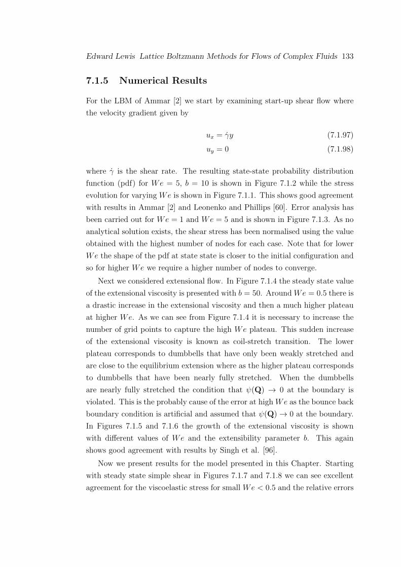
Edward Lewis Lattice Boltzmann Methods for Flows of Complex Fluids 133
7.1.5 Numerical Results
For the LBM of Ammar [2] we start by examining start-up shear flow where
the velocity gradient given by
ux = γy (7.1.97)
uy = 0 (7.1.98)
where γ is the shear rate. The resulting state-state probability distribution
function (pdf) for We = 5, b = 10 is shown in Figure 7.1.2 while the stress
evolution for varying We is shown in Figure 7.1.1. This shows good agreement
with results in Ammar [2] and Leonenko and Phillips [60]. Error analysis has
been carried out for We = 1 and We = 5 and is shown in Figure 7.1.3. As no
analytical solution exists, the shear stress has been normalised using the value
obtained with the highest number of nodes for each case. Note that for lower
We the shape of the pdf at state state is closer to the initial configuration and
so for higher We we require a higher number of nodes to converge.
Next we considered extensional flow. In Figure 7.1.4 the steady state value
of the extensional viscosity is presented with b = 50. Around We = 0.5 there is
a drastic increase in the extensional viscosity and then a much higher plateau
at higher We. As we can see from Figure 7.1.4 it is necessary to increase the
number of grid points to capture the high We plateau. This sudden increase
of the extensional viscosity is known as coil-stretch transition. The lower
plateau corresponds to dumbbells that have only been weakly stretched and
are close to the equilibrium extension where as the higher plateau corresponds
to dumbbells that have been nearly fully stretched. When the dumbbells
are nearly fully stretched the condition that ψ(Q) → 0 at the boundary is
violated. This is the probably cause of the error at high We as the bounce back
boundary condition is artificial and assumed that ψ(Q)→ 0 at the boundary.
In Figures 7.1.5 and 7.1.6 the growth of the extensional viscosity is shown
with different values of We and the extensibility parameter b. This again
shows good agreement with results by Singh et al. [96].
Now we present results for the model presented in this Chapter. Starting
with steady state simple shear in Figures 7.1.7 and 7.1.8 we can see excellent
agreement for the viscoelastic stress for small We < 0.5 and the relative errors

134
Figure 7.1.1: Start up shear flow shown for We = 1, We = 3 and We = 5with b = 10.
have been given in Tables 7.4 and 7.5. As we can see the relative error at
higher We for higher values of b is smaller. A significant source of error in our
method is the assumption that the pdf of configuration of the dumbbells is
close to equilibrium. In the Ammar model essentially utilises the fact that the
Fokker-Planck equation is an advection-diffusion equation in configurational
space which can be simulated by breaking momentum conservation in the
lattice Boltzmann framework. This means that like the Onishi model, this
model is only suitable for weak flows. In fact upon solving lattice Fokker-
Planck equation (7.1.49) for steady state simple shear we find that when
γλ >2(b+ 6)
8b√
3(7.1.99)
the discrete probability distribution functions are no longer valid as ψj /∈ [0, 1].
However, for weak flows the model developed in this Chapter is much more
computationally efficient when compared to the model by Ammar [2]. For
example with We = 0.1, b = 10 we find our method takes 0.0714s compared to
137.4993s to reach the steady state solution which is a very significant increase
in speed. It might be beneficial in the future when solving large viscoelastic
problems to use both methods depending on the local Weissenberg number.
In Figure 7.1.9 the time evolution of the shear stress for start up shear flow is
shown and shows good qualitative agreement with results by Ammar [2] and
Singh et al. [96].

Edward Lewis Lattice Boltzmann Methods for Flows of Complex Fluids 135
Figure 7.1.2: Shaded surface of the pdf for We = 5, b = 10
Couette Flow
The next set of results are for the full coupled flow problem of start-up plane
Couette flow. Across the channel we solve the evolution of the horizontal
velocity at 9 equally spaced points y = yk, k = 0, . . . , 8. The material and
flow parameters are given by b = 10, Re = 1, λ1 = 1 and β = 1/9. The
time step is chosen as a compromise between performance and stability and is
chosen to be ∆t = T/3000 with T = 10. We present results for the evolution
We 0.01 0.05 0.1 0.5 1Ammar 0.0071 0.0357 0.0714 0.3489 0.6580
Present work 0.0071 0.0357 0.0714 0.3571 0.7143% Diff. -0.1988 -0.0269 -0.0870 -2.3659 -8.5573
Table 7.4: Relative percentage errors in steady state shear stress with b = 10between Ammar and the method developed in this Chapter.

136
Figure 7.1.3: Error convergence for We = 1 and We = 5 with b = 10.
We 0.01 0.05 0.1 0.5 1Ammar 0.0096 0.0480 0.0961 0.4770 0.9332
Present work 0.0096 0.0481 0.0962 0.4808 0.9615% Diff. -0.4234 -0.0669 -0.0406 -0.7890 -3.0360
Table 7.5: Relative percentage errors in steady state shear stress with b = 100between Ammar and the method developed in this Chapter.
of the horizontal velocity component at the points y0, y2, y4, y6, y8 in Figure
7.1.10. Qualitative agreement with Leonenko and Phillips [60] is observed.
The velocity exhibits a strong overshoot followed by a weak undershoot before
converging on a steady state value at around t = 3. The overshoot is strongest
in the centre of the channel. The corresponding evolution of the shear stress
at the mid-point of the channel is shown in Figure 7.1.11 which shows good
agreement with the results by Leonenko and Phillips [60].
7.1.6 Discussion
In this chapter we have presented results for Lattice Boltzmann equation style
solvers for the Fokker-Planck equation for the FENE dumbbell model. The
model by Ammar [2] is robust under shear flows for a wide range of We but
requires large grid sizes to capture the high plateau at large We under exten-
sional flow, due to the artificiality of the bounce back condition.
To model complex viscoelastic flows it is necessary to couple the solver
for the polymeric stress with a solver for the solvent velocity. The procedure
follows an iterative process where first the governing equations for the velocity

Edward Lewis Lattice Boltzmann Methods for Flows of Complex Fluids 137
Figure 7.1.4: Steady state value of extensional viscosity with different We forb = 50.
and pressure are solved, then the polymeric stress tensor is evaluated at each
point in physical space and then the velocity and pressure are updated based
on the extra stress to the momentum equation. For the FENE dumbbell model
there is no closed form constitutive equation for the polymeric stress tensor
and therefore macroscopic simulation techniques cannot be employed. Based
on the solution of the Fokker-Planck equation in the mesoscopic stage, a meso-
macro numerical algorithm is described. This has been demonstrated for start-
up plane Couette flow. Excellent agreement is obtained with the results by
Leonenko and Phillips [60]. For large physical domains this is computationally
expensive but with proper hardware implementation deserves attention in the
framework of numerical methods for complex fluids.
In the model developed in this chapter, we have attempted to solve the
Fokker-Planck equation using a single lattice to span both configurational and
physical spaces. The LBM of Ammar [2] and Singh et al. [96] use a sepa-

138
rate lattice to span the configurational space for each point in physical space.
Using a single lattice achieves a significant reduction in computation time.
For small We < 0.5 the present model is capable of replicating the results by
Ammar [2] and Singh et al. [96] for shear flow and computationally takes a
small fraction of the time to reach a steady state solution (0.0714s compared to
137.4993s). As the method by Ammar [2] requires the Fokker-Planck equation
to be solved at each physical point in space, this would lead to an even more
significant reduction in computation time when used to solve for large physical
domains. However, the assumption that the distribution functions can be ex-
panded about the equilibrium solution means that our method is only suitable
for weak flows We < 0.5. It might be therefore beneficial to investigate a dual
approach if solving flows with a mixture of large and small values of the local
We to achieve the best of both approaches.

Edward Lewis Lattice Boltzmann Methods for Flows of Complex Fluids 139
(a) b=20
(b) b=50
(c) b=100
Figure 7.1.5: Time evolution of the extensional viscosity for We = 0.3.

140
(a) b=20
(b) b=50
(c) b=100
Figure 7.1.6: Time evolution of the extensional viscosity for We = 3.0.
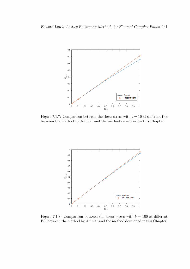
Edward Lewis Lattice Boltzmann Methods for Flows of Complex Fluids 141
Figure 7.1.7: Comparison between the shear stress with b = 10 at different Webetween the method by Ammar and the method developed in this Chapter.
Figure 7.1.8: Comparison between the shear stress with b = 100 at differentWe between the method by Ammar and the method developed in this Chapter.

142
Figure 7.1.9: Time evolution of shear stress with b = 10 using the presentmodel.
Figure 7.1.10: Time evolution of the horizontal component of velocity at differ-ent locations for the start-up plane Couette flow of a FENE fluid with b = 10,λ1 = 1 and T = 10.

Edward Lewis Lattice Boltzmann Methods for Flows of Complex Fluids 143
Figure 7.1.11: Time evolution of shear stress at the mid-channel location forthe start-up plane Couette flow of a FENE fluid with b = 10, λ1 = 1 andT = 10.
Chapter 8
Conclusions and future Work
The lattice Boltzmann method is a relatively new technique in computational
fluid dynamics based on the resolution of physics at a mesoscopic level. It
has already had many successes in solving many different flow scenarios such
multi-phase fluid flows or flow through porous media and the aim of this thesis
was to expand on this success into solving viscoelastic flows.
Chapter 1 is an introduction into LBM and put it into context based on
other macroscopic fluid solvers and the LGCA which was its direct forebear.
It is important to remember that there is no numerical scheme that is the best
at solving every problem and attempts were made to highlight areas where
LBM have significant advantages over traditional macroscopic solvers such as
FDM or FEM.
Chapter 2 explains how to implement a LBM scheme. The collision al-
gorithm is discussed and the two main approximations BGK and MRT are
given. In practice the BGK is far more popular due to its ease of use but
MRT has significant advantages for studying more complicated flows as there
are non-physical parameters that can be tuned to improve stability. When
solving large systems the propagation algorithm used can have a significant
difference to the speed of the overall LBM. A more efficient implementation of
the propagation algorithm in terms of the memory required is given. However,
on modern computer architectures it has been found to be significantly slower
than a two array approach. A major advantage of the LBM over traditional
macroscopic fluid velocity solvers is the ease of implementation of boundary
conditions. In LBM boundary conditions are applied locally and so it is very
144
Edward Lewis Lattice Boltzmann Methods for Flows of Complex Fluids 145
simple to describe fluid flow in complex geometries such as porous media. The
so called bounce-back condition is used to simulate no-penetration and no-slip
condition at a boundary. The two major versions of the bounce-back con-
dition, (on grid and mid grid) are described and results are presented as to
the increase in accuracy from using the mid grid condition for Poiseuille flow.
Zou-He [106] developed a constant velocity/pressure boundary condition that
is second order accurate based on the assumption that the bounce back rule
holds for the non-equilibrium part of the particle distribution function normal
to the boundary and results are presented for the D2Q7 and D2Q9 lattice for
Couette flow using the Zou-He constant velocity condition.
In Chapter 3 the derivation of the equilibrium distribution function is pre-
sented in two ways. Firstly it is given as a discretised version of the Maxwell-
Boltzmann equilibrium distribution using Gauss-Hermite quadrature and sec-
ondly it is constructed from the macroscopic properties required and using
them to solve the linear system to recover the coefficients of the equilibrium
function. Also in Chapter 3 is the relation between the LBM and Navier-Stokes
equations which is given by the Chapman-Enskog multi-scale procedure. Chap-
ter 3 is vital when looking for ways to adapt the LBM to solve other problems
such as the Fokker-Planck equation as shown in Chapter 7.
In Chapter 4 an overview of LBM for multiphase fluid flows is given. The
four main approaches are chromodynamic models, pseudo-potential models,
free-energy models and mean field models. Free energy and mean field models
are necessary when examining non-isothermal flows but are computationally
expensive and are not able to solve fluid flows with a large density ratio.
Pseudo-potential models are easy to implement as they require adding a body
force term to the LBM and are capable of simulating fluids with a high density
ratio but have relatively low numerical stability and wide diffuse interfaces
between the fluids. The colour model is capable of simulating fluids with a
significant viscosity ratio and recovers the analytic solutions for Poiseuille flow
and fingering simulations. In this Chapter the colour model is used to solve two
and three layer Poiseuille flow and gives good agreement with the analytical
solutions.
In Chapter 5 a LBM for droplets is discussed. Lattice Boltzmann methods
are extremely well suited to modelling the behaviour of droplets on surfaces

146
since only the static contact angles are needed to simulate the impingement
and spreading of droplets as the dynamic contact angle emerges naturally from
the simulation without complicated treatment. In the context of real world
applications this allows the LBM to be easily calibrated to match experimental
results. The static contact angles can be measured by placing a droplet on a
surface and tilting the surface until the droplet starts to move and measuring
the advancing and receding contact angles relative to the surface. This then
allows more complicated droplet flows to be studied numerically.
In Chapter 6 an overview of LBM for viscoelastic flows is presented. The
multi-relaxation models for non-Newtonian LBE’s proposed by Giraud et al.
[31, 32] take advantage of the LB framework by incorporating viscoelastic ef-
fects into the collision operator so that characteristic quantities of complex
fluids are given purely in terms of lattice moments. The ability to ‘tune’ the
collision matrix gives these models the potential to recover the constitutive
equation of choice without having to resort to additional numerical differenti-
ation of macroscopic quantities such as the velocity gradient. This theoretical
advantage has yet to be demonstrated correctly in practice and the relation
between the viscoelastic properties and lattice moments is not well understood
at present. The lattice Fokker-Planck models on the other hand have a firm
mathematical basis as they are shown to be a direct discretisation of the con-
tinuous kinetic equation.
In Chapter 7 two lattice based approaches are used to solve the Fokker-
Planck equation with the FENE force law. The method by Ammar [2] and
Singh et al. [96] is presented and shows excellent agreement with other FENE
solvers. This method though requires solutions to be generated on separate
lattices since a separate Fokker-Planck equation at every position in physical
space needs to be solved which is computationally expensive. Taking the work
by Onishi et al. [75] as an inspiration the Fokker-Planck equation with a FENE
force law was discretised using only one lattice for the whole physical space.
This gives a dramatic increase in computational efficiency in terms of both
memory and processing power. However, in deriving our model we assume that
the distribution functions can be expanded about the equilibrium distribution
and for strong flows this assumption does not hold. Therefore while our model
is dramatically faster at computing polymeric stresses at small values of the

Edward Lewis Lattice Boltzmann Methods for Flows of Complex Fluids 147
Weissenberg number (We < 0.5) it is unable to accurately capture polymeric
behaviour for larger values of We. This contribution is being prepared for
submission to Physical Review E. [61]. The start-up of plane Couette flow is
considered. A numerical method for solving this problem based on a coupling
of the method by Ammar [2] and a solver for macroscopic fluid velocity as
been performed and shows excellent agreement for the temporal evolution of
both the solvent velocity and the shear stress with the results by Leonenko
and Phillips [60].
Future work involves capitalising on the success and features of the LBM
by coupling our method for solving for the Fokker-Planck equation with the
FENE force law, with a LBM for multiphase fluid flow. A current drawback
to our approach is that is unable to accurately capture polymeric behaviour at
larger values of We. Currently there a two ideas to improve or mitigate this
drawback. Firstly it is worth investigating using more lattice speeds (corre-
sponding to using more nodes in the Gaussian quadrature) when performing
the discretisation. Presently the model expands the pdf about the equilibrium
solution and adding more terms into this expansion should increase the range
of permissible values of We. Secondly a hybrid approach may be adopted
where at smaller values of We our model is used to solve for the polymeric
stress and at higher values of We where our approach breaks down, use the
LBM of Ammar [2]. This should deliver a considerable increase in the overall
speed of solution of the polymeric stress. A distinct advantage of the LBM
for multiphase fluid flow is for simulating droplets on surfaces, and so it is
proposed to couple our method for computing the viscoelastic stresses with a
LBM for droplets to simulate the flow of droplets of polymeric liquids on sur-
faces. This has industrial applications including ink-jet printing where many
dyes and paints are viscoelastic.

Bibliography
[1] T. Abe, Derivation of the lattice Boltzmann method by means of the
discrete ordinate method for the Boltzmann equation, J Comput Phys,
131 (1997), pp. 241–246.
[2] A. Ammar, Lattice Boltzmann method for polymer kinetic theory, J
Non-Newton Fluid, 165 (2010), pp. 1082–1092.
[3] Y. Ba, H. Liu, J. Sun, and R. Zheng, Color–gradient lattice Boltz-
mann model for simulating droplet motion with contact angle hysteresis,
Phys Rev E, 88 (2013), p. 043306.
[4] J. Bernsdorf, S. Harrison, S. Smith, P. Lawford, and
D. Hose, Applying the lattice Boltzmann technique to biofluids: A novel
approach to simulate blood coagulation, Comput Math Appl, 55 (2008),
pp. 1408 – 1414. Mesoscopic Methods in Engineering and Science.
[5] P. L. Bhatnagar, E. P. Gross, and M. Krook, A model for col-
lision processes in gases. i. small amplitude processes in charged and
neutral one-component systems, Phys Rev, 94 (1954), pp. 511–525.
[6] C. Binetruy, F. Chinesta, and R. Keunings, Flows in Polymers,
Reinforced Polymers and Composites: A Multi-scale approach, Springer,
Cham, 2015.
[7] R. Bird, R. Armstrong, and O. Hassager, Dynamics of Polymeric
Liquids, Volume 1: Fluid Mechanics, 2nd edition, Wiley, New York,
1987.
148

Edward Lewis Lattice Boltzmann Methods for Flows of Complex Fluids 149
[8] R. Bird, C. Curtiss, R. Armstrong, and O. Hassager, Dynamics
of Polymeric Liquids, Volume 2: Fluid Mechanics, 2nd edition, Wiley,
New York, 1987.
[9] T. Blake, The physics of moving wetting lines, J Colloid Interface Sci,
299 (2006), pp. 1 – 13.
[10] J. Castrejon-Pita, K. Kubiak, A. Castrejon-Pita, M. Wilson,
and I. Hutchings, Mixing and internal dynamics of droplets impacting
and coalescing on a solid surface, Phys Rev E, 8 (2013), p. 023023.
[11] J. R. Castrejon-Pita, E. S. Betton, K. J. Kubiak, M. C. T.
Wilson, and I. M. Hutchings, The dynamics of the impact and
coalescence of droplets on a solid surface, Biomicrofluidics, 5 (2011).
[12] C. Cercignani, The Boltzmann Equation and its Applications, New
York: Springer, 1988.
[13] S. Chapman and T. G. Cowling, The Mathematical Theory of Non-
Uniform Gases, 3rd ed., Cambridge Mathematical Library, Cambridge,
1970, ch. 16.
[14] H. Chen, B. Boghosian, P. Coveney, and M. Nekovee, A
Ternary Lattice Boltzmann Model for Amphiphilic Fluids, PHILOS T
ROY SOC A, 456 (2000), pp. 2043–2057.
[15] H. Chen, S. Chen, and W. Matthaeus, Recovery of the Navier-
Stokes equations using a lattice-gas Boltzmann method, Phys Rev A, 45
(1992), pp. R5339–R5342.
[16] S. Chen, H. Chen, D. Martinez, and W. Matthaeus, Lattice
Boltzmann model for simulation of magnetohydrodynamics, Phys Rev
Lett, 67 (1991), p. 3776.
[17] S. Chen and D. G., Lattice Boltzmann method for fluid flows, Annu
Rev Fluid Mech, 30 (1998), pp. 329–364.

150
[18] S. Chen, X. He, and L.-S. Luo, Lattice Boltzmann models for mul-
tiphase flows, in Computational Methods for Multiphase Flow, A. Pros-
peretti and G. Tryggvason, eds., Cambridge University Press, 2007,
pp. 157–192.
[19] X.-P. Chen, Applications of lattice Boltzmann method to turbulent flow
around two-dimensional airfoil, Eng Appl Comput Fluid Mech, 6 (2012),
pp. 572–580.
[20] I.-L. Chern, J. Glimm, O. McBryan, B. Plohr, and S. Yaniv,
Front tracking for gas dynamics, J Comput Phys, 62 (1986), pp. 83–110.
[21] M. Creutz, Quarks, Gluons and Lattices, Cambridge University Press,
Cambridge, 1983.
[22] P. G. de Gennes, Wetting: statics and dynamics, Rev Mod Phys, 57
(1985), pp. 827–863.
[23] P. J. Dellar, Bulk and shear viscosities in lattice Boltzmann equations,
Phys. Rev. E, 64 (2001), p. 031203.
[24] C. Denniston, E. Orlandini, and J. M. Yeomans, Lattice Boltz-
mann simulations of liquid crystal hydrodynamics, Phys. Rev. E, 63
(2001), p. 056702.
[25] B. Derby, Inkjet printing of functional and structural materials: Fluid
property requirements, feature stability, and resolution, Annu Rev Mater
Sci, 40 (2010), pp. 395–414.
[26] D. d’Humieres, A. Cloquer, and P. Lallemand, Lattice gas mod-
els for 3d hydrodynamics, Europhys Lett, 25 (1986), p. 129.
[27] U. D’Ortona, D. Salin, M. Cieplak, R. B. Rybka, and J. R.
Banavar, Two-color nonlinear Boltzmann cellular automata: Surface
tension and wetting, Phys Rev E, 51 (1995), pp. 3718–3728.
[28] J.-B. Dupont and D. Legendre, Numerical simulation of static and
sliding drop with contact angle hysteresis, J Comput Phys, 229 (2010),
pp. 2453 – 2478.

Edward Lewis Lattice Boltzmann Methods for Flows of Complex Fluids 151
[29] S. Fathi and P. Dickens, Challenges in drop-on-drop deposition of
reactive molten nylon materials for additive manufacturing, J Mater Pro-
cess Tech, 213 (2013), pp. 84 – 93.
[30] U. Frisch, B. Hasslacher, and Y. Pomeau, Lattice gas automata
for the Navier-Stokes equations, Phys Rev Lett, 56 (1986), pp. 1505–
1508.
[31] L. Giraud, D. d’Humieres, and P. Lalleemand, A lattice Boltz-
mann model for viscoelasticity, Int. J. Mod. Phys. C,, 8 (1997), pp. 805–
815.
[32] , A lattice Boltzmann method for Jeffreys viscoelastic fluid, Euro-
phys. Lett, 42 (1998), pp. 625–630.
[33] J. Glimm, M. J. Graham, J. Grove, X. L. Li, T. M. Smith,
D. Tan, F. Tangerman, and Q. Zhang, Front tracking in two and
three dimensions, Comps Math Appl, 35 (1998), pp. 1–11.
[34] J. Glimm, J. W. Grove, X. L. Li, K.-m. Shyue, Y. Zeng, and
Q. Zhang, Three-dimensional front tracking, SIAM J Sci Comput, 19
(1998), pp. 703–727.
[35] J. Glimm, E. Isaacson, D. Marchesin, and O. McBryan, Front
tracking for hyperbolic systems, Adv Appl Math, 2 (1981), pp. 91–119.
[36] A. Gunstensen, D. H. Rothman, S. Zaleski, and G. Zanetti,
Lattice Boltzmann model of immiscible fluids, Phys Rev A, 43 (1991),
pp. 4320–4327.
[37] Z. Guo, C. Zheng, and B. Shi, Discrete lattice effects on the forcing
term in the lattice Boltzmann method, Phys Rev E, 65 (2002b), p. 046308.
[38] I. Halliday, A. P. Hollis, and C. M. Care, Lattice Boltzmann
algorithm for continuum multicomponent flow, Phys Rev E, 76 (2007),
p. 026708.
[39] F. H. Harlow and J. E. Welch, Numerical calculation of time-
dependent viscous incompressible flow of fluid with free surface, Phys
Fluids, 8 (1965), pp. 2182–2189.

152
[40] X. He, S. Chen, and G. Doolen, A Novel Thermal Model for the
Lattice Boltzmann Method in Incompressible Limit, J. Comp Phys, 146
(1998), pp. 282 – 300.
[41] X. He and G. Doolen, Thermodynamic foundation of kinectic theory
and lattice Boltzmann models for multiphase flows, J Stat Phys, 107
(2002), pp. 309–328.
[42] X. He and L. L-S, A priori derivation of the lattice Boltzmann equa-
tion, Phys Rev E, 57 (1997), pp. R6333–R6336.
[43] X. He, X. Shan, and G. Doolen, Discrete Boltzmann equation model
for nonideal gases, Phys Rev E, 57 (1998), pp. R13–R16.
[44] M. Herrchen and H. Ottinger, A detailed comparison of various
FENE dumbbell models, J Non-Newton Fluid, 68 (1997), pp. 17–42.
[45] F. Higuera and J. Jimenez, Boltzmann approach to lattice gas sim-
ulations, Europhys Lett, 9 (1989), p. 663.
[46] A. P. Hollis, T. J. Spencer, I. Halliday, and C. M. Care,
Dynamic wetting boundary condition for continuum hydrodynamics with
multi-component lattice Boltzmann equation simulation method, IMA J
Appl Math, 76 (2011), pp. 726–742.
[47] J. Horbach and D. Frenkel, Lattice-Boltzmann method for the sim-
ulation of transport phenomena in charged colloids, Phys. Rev. E, 64
(2001), p. 061507.
[48] R. R. Huilgol and N. Phan-Thien, Fluid Mechanics of Viscoelas-
ticity, Elsevier Science BV, Amsterdam, 1997.
[49] D. Humieres, Multiple–relaxation–time lattice Boltzmann models in
three dimensions, Philos T R Soc A, 360 (2002), pp. 437–451.
[50] T. Inamuro, T. Ogata, S. Tajima, and N. Konishi, A lattice
Boltzmann method for incompressible two-phase flows with large density
differences, J Comput Phys, 198 (2004), pp. 628–644.

Edward Lewis Lattice Boltzmann Methods for Flows of Complex Fluids 153
[51] K. Kadau, J. Barber, T. Germann, B. Holian, and B. Alder,
Atomistic methods in fluid simulation, Philos T Roy Soc A, 368 (2010),
pp. 1547–1560.
[52] J. Koelman, A simple lattice Boltzmann scheme for Navier-Stokes fluid
flow, Europhys Lett, 15 (1991), p. 603.
[53] T. Kruger, H. Kusumaatmaja, A. Kuzmin, O. Shardt,
G. Silva, and E. M. Viggen, The Lattice Boltzmann Method, Springer
International Publishing Switzerland, 2017.
[54] F. Kuznik and G. Rusaouen, Numerical prediction of natural con-
vection occurring in building components: A double-population lattice
Boltzmann method, Numer Heat Tr A-Appl, 52 (2007), pp. 315–335.
[55] A. J. Ladd, Lattice-Boltzmann methods for suspensions of solid parti-
cles, Mol Phys, 113 (2015), pp. 2531–2537.
[56] P. Lallemand and L.-S. Luo, Theory of the lattice Boltzmann
method: Dispersion, dissipation, isotropy, Galilean invariance, and sta-
bility., Phys. Rev. E., 61 (2000), pp. 6546–6562.
[57] M. Laso and H. Ottinger, Calculation of viscoelastic flow using
molecular models: the connffessit approach, J Non-Newton Fluid, 47
(1993), pp. 1 – 20.
[58] M. Latva-Kokko and D. Rothman, Diffusion properties of gradient-
based lattice Boltzmann models of immiscible fluids, Phys Rev E, 71
(2005), p. 056702.
[59] , Scaling of dynamic contact angles in a lattice-Boltzmann model,
Phys Rev Lett, 98 (2007), p. 254503.
[60] G. M. Leonenko and T. N. Phillips, The Prediction of Plane Cou-
ette Flow for a FENE Fluid Using a Reduced Basis Approximation of
the Fokker-Planc Equation, Int J Mult Comp Eng, 9 (2011), pp. 73–88.
[61] E. Lewis and T. N. Phillps, A Lattice Boltzmann Approach for the
FENE Dumbbell model, Phys Rev E, (2017). In preparation.

154
[62] S. V. Lishchuk, C. M. Care, and I. Halliday, Lattice Boltzmann
algorithm for surface tension with greatly reduced microcurrents, Phys
Rev E, 67 (2003), p. 036701.
[63] P. Love, M. Nekovee, P. Coveney, J. Chin, N. GonzA¡lez-
Segredo, and J. Martin, Simulations of amphiphilic fluids using
mesoscale lattice-Boltzmann and lattice-gas methods, Comput Phys Com-
mun, 153 (2003), pp. 340 – 358.
[64] A. Lozinski and C. Chauviere, A fast solver for Fokker-Planck equa-
tion applied to viscoelastic flows calculations: 2D FENE model, J Com-
put Phys, 189 (2003), pp. 607 – 625.
[65] A. Lozinski, R. Owens, and T. N. Phillips, The Langevin and
Fokker-Planck Equations in Polymer Rheology, in Numerical Methods
for Non-Newtonian Fluids, R. Glowinski and J. Xu, eds., Elsevier B.V.
Amsterdam, 2011, pp. 211–303.
[66] L. Luo and X. He., Theory of the lattice Boltzmann method: From
the Boltzmann equation to the lattice Boltzmann equation., Phys Rev E,
(1997), pp. 6811–6817.
[67] N. Martys and H. Chen, Simulation of multicomponent fluids in
complex three-dimensional geometries by the lattice Boltzmann method,
Phys Rev E, 53 (1996), pp. 743–750.
[68] K. Mattila, J. Hyvaluoma, T. Rossi, M. Aspnas, and J. West-
erholm, An efficient swap algorithm for the lattice Boltzmann method,
Comput Phys Commun, 176 (2007), pp. 200–210.
[69] G. McNamara and G. Zanetti, Use of the Boltzmann equation to
simulate lattice gas automata, Phys Rev Lett., 61 (1988), p. 2332.
[70] A. Mohamad and A. Kuzmin, A critical evaluation of force term in
lattice Boltzmann method, natural convection problem, Int, J. Heat Mass
Transfer, 53 (2010), pp. 990 – 996.

Edward Lewis Lattice Boltzmann Methods for Flows of Complex Fluids 155
[71] D. Moroni, B. Rotenberg, J.-P. Hansen, S. Succi, and S. Mel-
chionna, Solving the Fokker-Planck kinetic equation on a lattice, Phys
Rev E, 73 (2006), p. 066707.
[72] M. Nekovee, P. Coveney, H. Chen, and B. Boghosian, Lattice-
Boltzmann model for interacting amphiphilic fluids, Phys. Rev. E, 62
(2000), pp. 8282–8294.
[73] W. F. Noh and P. Woodward, SLIC (Simple Line Interface Calcula-
tion), Springer Berlin Heidelberg, Berlin, Heidelberg, 1976, pp. 330–340.
[74] OED Online, viscoelasticity, n., 2016. [Accessed March, 2016].
[75] J. Onishi, Y. Chen, and H. Ohashi, A lattice Boltzmann model for
polymeric liquids, Prog Comput Fluid Dy, 5 (2005), pp. 75–84.
[76] J. Onishi, A. Kawasaki, Y. Chen, and H. Ohashi, Lattice Boltz-
mann simulation of capillary interactions among colloidal particles,
Comput Math Appl, 55 (2008), pp. 1541 – 1553.
[77] P. Pavlo, G. Vahala, and L. Vahala, Higher order isotropic veloc-
ity grids in lattice methods, Phys Rev Lett, 80 (1998), pp. 3960–3963.
[78] A. Peterlin, Hydrodynamics of macromolecules in a velocity field with
longitudinal gradient, J. Polym. Sci. B, 4 (1966), pp. 287–291.
[79] N. Phan-Thien, Understanding Viscoelasticity: Basics of Rheology,
Advanced Texts in Physics, Springer Berlin Heidelberg, 2013.
[80] T. N. Phillips and R. Owens, Computational Rheology, Imperial
College Press, London, 2002.
[81] T. N. Phillips and G. Roberts, Lattice Boltzmann models for non-
Newtonian flows, IMA J Appl Math, 76 (2011), pp. 790–816.
[82] Y. Qian, D. d’Humieres, and P. Lallemand, Lattice BGK models
for the Navier-Stokes equation, Europhys Lett, 17 (1992), p. 479.
[83] L. E. Reichl, A Modern Course in Statistical Physics, John Wiley &
Sons, Inc, New York, 1998.

156
[84] T. Reis, The Lattice Boltzmann Method for Complex Flows, PhD thesis,
Cardiff University, School of Mathematics, August 2007.
[85] T. Reis and T. N. Phillips, Lattice Boltzmann model for simulating
immiscible two-phase flows, J Phys A-Math Theor, 40 (2007a), pp. 4033–
4053.
[86] M. Renardy, Y. Renardy, and J. Li, Numerical simulation of mov-
ing contact line problems using a volume-of-fluid method, J Comput
Phys, 171 (2001), pp. 243 – 263.
[87] J. Rivet and J. Boon, Lattice Gas Hydrodynamics, Cambridge Uni-
versity Press, Cambridge, 2001.
[88] D. Rothman and J. Keller, Immiscible cellular-automaton fluids, J
Stat Phys, 52 (1988), pp. 1119–1127.
[89] J. S. Rowlinson and B. Widom, Molecular Theory of Capillarity,
Oxford University Press, Oxford, 1982.
[90] R. Scardovelli and S. Zaleski, Direct Numerical simulation of free-
surface and interfacial flow, Annu Rev Fluid Mech, 31 (1999), pp. 567–
603.
[91] J. D. Schieber and H. C. Ottinger, The effects of bead inertia on
the Rouse model, J Chem Phys, 89 (1988), pp. 6972–6981.
[92] A. D. Schleizer and R. T. Bonnecaze, Displacement of a two-
dimensional immiscible droplet adhering to a wall in shear and pressure-
driven flows, J Fluid Mech, 383 (1999), pp. 29–54.
[93] M. Seaton, R. Anderson, S. Metz, and W. Smith, DL MESO:
highly scalable mesoscale simulations, Mol Simulat, 39 (2013), pp. 796–
821.
[94] M. Sellier and E. Trelluyer, Modeling the coalescence of sessile
droplets, Biomicrofluidics, 3 (2009), p. 022412.

Edward Lewis Lattice Boltzmann Methods for Flows of Complex Fluids 157
[95] X. Shan and H. Chen, Lattice Boltzmann model for simulating flows
with multiple phases and components, Phys Rev E, 47 (1993), pp. 1815–
1819.
[96] S. Singh, G. Subramanian, and S. Ansumali, Lattice Fokker
Planck for dilute polymer dynamics, Phys Rev E, 88 (2013), p. 013301.
[97] P. A. Skordos, Initial and boundary conditions for the lattice Boltz-
mann method, Phys Rev E, 48 (1993), pp. 4823–4842.
[98] H. Song, H.-W. Li, M. Munson, T. Van Ha, and R. Ismagilov,
On–chip titration of an anticoagulant argatroban and determination of
the clotting time within whole blood or plasma using a plug-based mi-
crofluidic system, Anal Chem, 78 (2006), pp. 4839–4849.
[99] P. Spelt, A level-set approach for simulations of flows with multiple
moving contact lines with hysteresis, J Comput Phys, 207 (2005), pp. 389
– 404.
[100] S. Succi, The Lattice Boltzmann Equation for Fluid Dynamics and Be-
yond, Oxford University Press, Oxford, 2001.
[101] M. Swift, W. R. Osborn, and J. M. Yeomans, Lattice Boltzmann
simulation of nonideal fluids, Phys Rev Lett, 75 (1995), pp. 830–833.
[102] R. I. Tanner, Engineering Rheology, Oxford University Press, Oxford,
2002.
[103] J. Yang and E. Boek, A comparison study of multi-component lattice
Boltzmann models for flow in porous media applications, Comput Math
Appl, 65 (2013), pp. 882–890.
[104] X. Yang, V. H. Chhasatia, J. Shah, and Y. Sun, Coalescence,
evaporation and particle desposition of consecutively printed colloidal
drops, Soft Matter, 8 (2012), pp. 9205–9213.
[105] D. Ziegler, Boundary conditions for lattice Boltzmann simulations, J
Stat Phys, 71 (1993), pp. 1171–1177.

158
[106] Q. Zou and X. He, On pressure and velocity boundary conditions for
the lattice Boltzmann BGK model, Phys Fluids, 9 (1997), pp. 1591–1598.