computers & fluids improving lattice boltzmann simulation...

Computers & Fluids 00 (2014) 1–21

Computers& Fluids

Improving lattice Boltzmann simulation of moving particles in aviscous flow using local grid refinement

Songying Chena,∗, Cheng Pengb, Yihua Tengc, Lian-Ping Wangb,d

aSchool of Mechanical Engineering, Shandong University, Jinan, 250062, P.R. ChinabDepartment of Mechanical Engineering, 126 Spencer Laboratory, University of Delaware, Newark, Delaware 19716-3140, USA

cDepartment of Energy and Resource Engineering, Peking University, Beijing, P.R. ChinadNational Laboratory of Coal Combustion, Huazhong University of Science and Technology, Wuhan, P.R. China

Abstract

Accurate simulations of moving particles in a viscous flow require an adequate grid resolution near the surface of a moving particle.Within the framework of lattice Boltzmann approach, inadequate grid resolution could also lead to numerical instability and largefluctuations of the computed hydrodynamic force and torque. Here we explore the use of local grid refinement around a movingparticle to improve the simulation results using the multiple-relaxation-time (MRT) lattice Boltzmann method (LBM). We firstre-examine the necessary relationships, within MRT LBM, between the relaxation parameters and the distribution functions onthe coarse and fine grids, in order to meet the physical requirements of the fluid hydrodynamics and additional relationships asimplied by the Chapman-Enskog multi-scaling analysis. Several aspects of the implementation details are discussed, includingthe treatment of interface buffer nodes, the method to transfer information between the the coarse domain and fine domain, andthe computation of macroscopic variables including stress components. Our approach is then applied in two numerical tests todemonstrate that the local grid refinement can significantly improve the physical results with a high computational efficiency. Wecompare simulation results from three grid configurations: a uniformly coarse grid, a uniformly coarse grid with local refinement,and a uniformly fine grid. For the lid-driven cavity flow, the local refinement essentially yields local flow field that is comparableto the use of uniformly fine grid, but with a much less computational cost. In the Couette flow with a moving cylinder, thelocal refinement suppresses the level of force fluctuations. It was also found that the coarse-fine grid relationships between thenon-equilibrium moments of energy square and energy fluxes do not affect the simulation results.

c© 2011 Published by Elsevier Ltd.

Keywords: lattice Boltzmann method, local grid refinement, moving particles, force fluctuation, viscous flow

1. Introduction

As a highly efficient and capable mesoscopic computational method, the lattice Boltzmann method (LBM) [1, 2,3, 4] has been widely employed to solve a variety of fluid dynamics problems. LBM describes the fluid as makingup by imaginative elements which can stream along a uniform lattice grid and collide with one another only at latticenodes. The method solves a quasi-linear collision-streaming equation for a set of distribution functions associated

∗Corresponding author.Email address: [email protected] (Songying Chen), [email protected] (Chen Peng), [email protected]

(Yihua Teng), [email protected] (Lian-Ping Wang)

1

/ Computers & Fluids 00 (2014) 1–21 2

with discrete microscopic velocities. The macroscopic hydrodynamic variables such as pressure and velocity areobtained by taking the moments of the distribution functions.

One of the popular LBM schemes is based on the single relaxation time approach (i.e., Bhatnagar-Gross-Krookcollision process [5]), which is known as the LBGK model. Another popular scheme is based on the multiple-relaxation-time (MRT) collision model [6, 7]. The MRT collision is performed in the moment space with differentmoments relaxing at different rates. By decomposing the particle relaxation process into several independent re-laxation processes, the MRT model has been shown to not only improve the computational stability but also theaccuracy [6, 7, 8].

In order to obtain accurate macroscopic quantities, such as force and torque acting on a solid particle or theboundary, small grid spacing is needed near the solid particle or a boundary. Away from the boundary or fluid-solidinterfaces, the flow may be more smooth so a coarser grid is adequate to resolve the flow. The most efficient approachin terms of both memory and overall accuracy is thus to use a coarse grid for most of the bulk flow region, combinedwith a local grid refinement near a fluid-solid interface or wall boundary.

Within the LBGK model, local grid refinement has been considered for some time to simulate incompressibleviscous flows with complex geometries. Filippova and Hanel [9] was among the first to consider patching certainregions with a fine grid in a domain mostly covered by a coarse grid, values of the distribution functions on thecoarse grid which are coming from the fine patches are calculated on the nodes common to both grids. Filippova andHanel [10] presented an accelerated implementation of grid refinement by using different molecular speeds on thecoarse and fine grids. A smaller time step size was used on the fine grid while the spatial or temporal accuracy waskept. Steady-state and time-dependent problems were studied and the CPU time per time step was reduced by about50%.

Yu et al. [11] proposed a multi-block technique with the BGK model in LBM. Different mesh sizes are used fordifferent blocks that do not overlap. Macro-variables such as mass, momentum, and stress components are assumedto be continuous across the block-block interface, and this condition determines the relaxation parameters in the finedomain. The cubic spline scheme was used for spatial interpolation and the three-point Lagrangian formula was usedfor temporal interpolation on all nodes at the fine block boundary after the distribution functions are transferred fromthe coarse domain to the fine domain. Yu and Girimaji [12] extended their approach to 3D using the LBGK model.Two 3D test cases, an isotropic decaying turbulence and a lid-driven cavity flow, were presented to show the improvedcomputational efficiency.

Eitel-Amor et al. [13] introduced a cell-centered lattice structure to reconstruct the pre-collision distribution func-tions via spatial interpolation in LBGK model. They showed that, with hierarchically refined meshes, each cell canbe refined or coarsened regardless of the refinement level of neighbor cells. Lagrava [14] introduced a decimationtechnique to guarantee the stability of the numerical scheme especially at high flow Reynolds number when the infor-mation is transferred from the coarse nodes to the fine nodes. Dietzel and Sommerfeld [15] calculated flow resistanceover agglomerates with different morphology through LBGK local grid refinement. They slightly overlapped thecoarse and fine regions and designed a method to communicate the distribution functions between the two grids atthe interface. Premnath et al. [16] presented a staggered mesh arrangement in large-eddy simulation of a complexturbulent separated flow, using the MRT D3Q19 model. Subgrid scale model was employed in conjunction with theMRT to augment the relaxation time scales of hydrodynamic modes that allowed better representation of the effect ofsubgrid scale fluid motion.

The first attempt to implement local grid refinement within MRT was performed by Peng et al. [17] using theD2Q9 model, where they related the distribution functions and relaxation parameters in the two domains based onthe continuity of macro-variables at the coarse-fine interface. The method to communicate distributions functionsbetween the two domains was derived. They used lid-driven cavity flow, steady and unsteady flows past a circularcylinder, and flow over an airfoil to validate their approach. As will be shown later in this paper, their implementationwas not fully consistent since they ignored the relationship of energy relaxation parameters in the two domains.

It appears that the full details for implementing local grid refinement within the MRT model have not been care-fully studied. Our first objective is to re-examine the details of coupling the distribution functions and model pa-rameters between the fine and course grids within the MRT framework. Our second objective is to test local gridrefinement in moving particle simulation. In Section 2, a brief background description of the D2Q9 MRT model isprovided. Details of local grid refinement implementation are discussed in Section 3, together with the developmentof relationships between the course and fine grid. Necessary interpolation details at the coarse-fine interface are pre-

2


sented in Section 4. In section 5, we then validate our methodology using 2D lid-driven cavity flow, a Couette flowwith a fixed or a moving cylinder. In the case of moving cylinder, the refined region also moves with the cylinder. Testresults demonstrate that local grid refinement indeed improve the accuracy in moving particle simulation. We alsocompare CPU time and memory consumption when different grid arrangements (e.g., hybrid coarse / fine grid versusuniformly fine) are used. Key conclusions are summarized in Section 6.

2. The multiple-relaxation-time lattice Boltzmann method

Figure 1: The D2Q9 model with nine discrete velocities on two dimensional square lattice.

In this section, we briefly introduce the multiple-relaxation-time (MRT) lattice Boltzmann method (LBM) inorder to prepare for the discussions on the local grid refinement. The detailed description of MRT LBM can be foundin [6, 7].

Specifically the D2Q9 model [18, 19] is considered (Fig. 1), with discrete velocities given by:

ei ={(0, 0) (1, 0) (0, 1) (−1, 0) (0,−1) (1, 1) (−1, 1) (−1,−1) (1,−1)

}c. (1)

where i = 0, 1, 2, ..., 8, c = δx/δt. All variables are given in lattice units such that c = 1. The MRT LBM evolutionequation [6, 7] can be written as

f (x + eiδt, t + δt) = f (x, t) − M−1S[m −meq] . (2)

where f is a vector representing a set of distribution functions defined at a lattice node, m represents a set ofindependent moments, meq is the equilibrium of m, M is an orthogonal transformation matrix that transforms f intom

m = Mf, f = M−1m. (3)

The macroscopic hydrodynamic variables, including density ρ, velocity u =(ux, uy

), and pressure p are obtained

from the moments of the mesoscopic distribution function f. We use the nearly incompressible formulation, namely,the density is partitioned as ρ = ρ0 + δρ with ρ0 = 1, and δρ =

∑i fi, δρu =

∑i fiei, and p = δρc2

s , where cs = 1/√

3 isthe model speed of sound. For the D2Q9 MRT model, other moments and the transformation matrix are designed as

m =

ρeεjx

qx

jyqy

pxx

pxy

=

1 1 1 1 1 1 1 1 1−4 −1 −1 −1 −1 2 2 2 24 −2 −2 −2 −2 1 1 1 10 1 0 −1 0 1 −1 −1 10 −2 0 2 0 1 −1 −1 10 0 1 0 −1 1 1 −1 −10 0 −2 0 2 1 1 −1 −10 1 −1 1 −1 0 0 0 00 0 0 0 0 1 −1 1 −1

f0f1f2f3f4f5f6f7f8

. (4)

3


The three hydrodynamic moments, ρ, jx = ρ0ux, jy = ρ0uy, are locally conserved. The other six moments are notconserved, they are energy e, energy square ε, energy flux in x and y directions qx and qy, normal stress pxx, and shearstress pxy. These non-conserved moments are relaxed as follows

e = e − S e (e − eeq)

ε = ε − S ε (ε − εeq)

qx = qx − S q(qx − qeqx )

qy = qy − S q(qy − qeqy )

pxx = pxx − S ν(pxx − peqxx)

pxy = pxy − S ν(pxy − peqxy),

(5)

where the symbol ∼ denotes the post-collision value. The equilibriums of non-conserved moments are designed tomatch the Euler and Navier-Stokes equation through the Chapman-Enskog analysis, and the results are

eeq = −2δρ + 3ρ0u2

εeq = δρ − 3ρ0u2

qeqx = −ρ0ux

qeqy = −ρ0uy

peqxx = ρ0

(u2

x − u2y

)peq

xy = ρ0uxuy,

(6)

where u2 = u2x + u2

y . While the equilibrium εeq plays no role in the Navier-Stokes equation and thus its form can beflexible, the specific form stated above leads to the standard feq = M−1meq as

f eqi = wi

{δρ + ρ0

[ei · u

c2s

+(ei · u)2

2c4s−

u · u2c2

s

]}. (7)

where the weighting coefficient wi is given as

w0 =49, wi =

19

(i = 1, 2, 3, 4), wi =136

(i = 5, 6, 7, 8) . (8)

It follows that the diagonal relaxation matrix S is

S = Diag[0 S e S ε 0 S q 0 S q S ν S ν

]. (9)

The shear viscosity and bulk viscosity in the MRT model can be derived from the Chapman-Enskog analysis as

ν = c2s

(1

S ν− 0.5

)δt

ξ = c2s

(1

S e− 0.5

)δt.

(10)

The evolution equation for f can be divided into two sub-steps: collision and streaming, as

f (x, t) = f (x, t) − M−1S[m −meq] , (11)

f (x + eiδt, t + δt) = f (x, t) . (12)

In summary, the key features of the MRT model is that collision is performed in the moment space, and streamingoccurs in the discrete-velocity space. The two relaxation times S ν and S e determine the shear and bulk viscosity, theother two relaxation parameters S q and S ε may be viewed as free parameters that can be used to improve the accuracyof boundary condition or to enhance numerical stability [6].

4


3. Local grid refinement implementation in MRT LBM

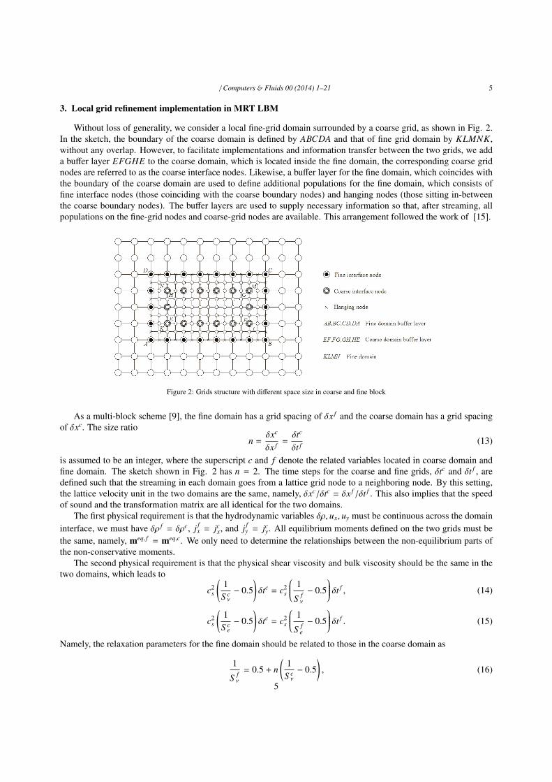
Without loss of generality, we consider a local fine-grid domain surrounded by a coarse grid, as shown in Fig. 2.In the sketch, the boundary of the coarse domain is defined by ABCDA and that of fine grid domain by KLMNK,without any overlap. However, to facilitate implementations and information transfer between the two grids, we adda buffer layer EFGHE to the coarse domain, which is located inside the fine domain, the corresponding coarse gridnodes are referred to as the coarse interface nodes. Likewise, a buffer layer for the fine domain, which coincides withthe boundary of the coarse domain are used to define additional populations for the fine domain, which consists offine interface nodes (those coinciding with the coarse boundary nodes) and hanging nodes (those sitting in-betweenthe coarse boundary nodes). The buffer layers are used to supply necessary information so that, after streaming, allpopulations on the fine-grid nodes and coarse-grid nodes are available. This arrangement followed the work of [15].

Figure 2: Grids structure with different space size in coarse and fine block

As a multi-block scheme [9], the fine domain has a grid spacing of δx f and the coarse domain has a grid spacingof δxc. The size ratio

n =δxc

δx f =δtc

δt f (13)

is assumed to be an integer, where the superscript c and f denote the related variables located in coarse domain andfine domain. The sketch shown in Fig. 2 has n = 2. The time steps for the coarse and fine grids, δtc and δt f , aredefined such that the streaming in each domain goes from a lattice grid node to a neighboring node. By this setting,the lattice velocity unit in the two domains are the same, namely, δxc/δtc = δx f /δt f . This also implies that the speedof sound and the transformation matrix are all identical for the two domains.

The first physical requirement is that the hydrodynamic variables δρ, ux, uy must be continuous across the domaininterface, we must have δρ f = δρc, j f

x = jcx, and j fy = jcy. All equilibrium moments defined on the two grids must be

the same, namely, meq, f = meq,c. We only need to determine the relationships between the non-equilibrium parts ofthe non-conservative moments.

The second physical requirement is that the physical shear viscosity and bulk viscosity should be the same in thetwo domains, which leads to

c2s

(1

S cν

− 0.5)δtc = c2

s

1

S fν

− 0.5 δt f , (14)

c2s

(1

S ce− 0.5

)δtc = c2

s

1

S fe

− 0.5 δt f . (15)

Namely, the relaxation parameters for the fine domain should be related to those in the coarse domain as

1

S fν

= 0.5 + n(

1S cν

− 0.5), (16)

5


1

S fe

= 0.5 + n(

1S c

e− 0.5

). (17)

The third physical requirement is that the normal and shear stress components should be the same at the domaininterface. The Chapman-Enskog analysis states that

τxx = −16

(1 − 0.5S e) eneq −12

(1 − 0.5S ν) pneqxx

τyy = −16

(1 − 0.5S e) eneq +12

(1 − 0.5S ν) pneqxx

τxy = − (1 − 0.5S ν) pneqxy .

(18)

Therefore, we demand

−16

(1 − 0.5S c

e)

eneq,c −12

(1 − 0.5S c

ν

)pneq,c

xx = −16

(1 − 0.5S f

e

)eneq, f −

12

(1 − 0.5S f

ν

)pneq, f

xx , (19)

−16

(1 − 0.5S c

e)

eneq,c +12

(1 − 0.5S c

ν

)pneq,c

xx = −16

(1 − 0.5S f

e

)eneq, f +

12

(1 − 0.5S f

ν

)pneq, f

xx , (20)

−(1 − 0.5S c

ν

)pneq,c

xy = −(1 − 0.5S f

ν

)pneq, f

xy . (21)

Solving these three equations and in view of the conditions given by Eqs. (16) and (17), we obtain the followingrelationships between three non-equilibrium moments in the two domains, as

eneq, f =S c

e

nS fe

eneq,c, pneq, fxx =

S cν

nS fν

pneq,cxx , pneq, f

xy =S cν

nS fν

pneq,cxy . (22)

For the three remaining non-equilibrium moments: energy square and two energy flux components, the Chapman-Enskog analysis shows that

∂t1

(δρ − 3ρ0u2

)+ ∂1x (−ρ0ux) + ∂1y

(−ρ0uy

)= −

S εεneq

dt, (23)

∂t1 (−ρ0ux) + ∂1x

(−1 + 6u2

y − 3u2)

+ ∂1y

(ρ0uxuy

)= −

S qqneqx

dt, (24)

∂t1

(−ρ0uy

)+ ∂1x

(ρ0uxuy

)+ ∂1y

(−1 + 6u2

x − 3u2)

= −S qqneq

y

dt. (25)

The left hand sides involve only the hydrodynamic variables and should be the same when defined on the two grids,therefore, we set

S cεε

neq,c

dtc =S fεε

neq, f

dt f , (26)

S cqqneq,c

x

dtc =S f

q qneq, fx

dt f , (27)

S cqqneq,c

y

dtc =S f

q qneq, fy

dt f . (28)

The two remaining relaxation parameters, S ε and S q, do not enter the Navier-Stokes equation and can be treatedarbitrarily. For convenience, we simple assume that these two relaxation parameters are the same in the two gridsystems, namely, S f

ε = S cε and S f

q = S cq. Then Eqs. (26-28) becomes

εneq,c = nεneq, f , qneq,cx = nqneq, f

x , qneq,cy = nqneq, f

y . (29)

6


At this point, all necessary relationships are worked out for constructing distribution functions and model param-eters on the fine grid from those on the coarse grid, and vice versa. They can be summarized as follows

meq,c = meq, f and mneq,c ≡

ρ − ρeq

e − eeq

ε − εeq

jx − jeqx

qx − qeqx

jy − jeqy

qy − qeqy

pxx − peqxx

Pxy − peqxy

c

=

1nS f

e

S ce

n1

n1

nnS f

ν

S cν

nS fν

S cν

mneq, f . (30)

Therefore, we can introduce the following notations

mneq,c = T f mneq, f , mneq, f = T cmneq,c, (31)

where

T f = diag[1

nS fe

S ce

n 1 n 1 nnS f

ν

S cν

nS fν

S cν

], (32)

T c = diag[1

S ce

nS fe

1n

11n

11n

S cν

nS fν

S cν

nS fν

]. (33)

We shall now explain how to obtain the post-collision distribution function on a fine grid in terms of the post-collision distribution function on a coarse grid. First, the post-collision distribution function on the fine grid is deter-mined as

f f = f f − M−1S f(m f −meq, f

)= M−1m f − M−1S f

(m f −meq, f

), (34)

which, after substituting Eq. (31), becomes

f f = M−1meq, f + M−1(I − S f

)T cmneq,c. (35)

On the other hand, the post-collision moments in the coarse domain can be expressed as

Mfc = mc − S c (mc −meq,c) = meq,c + (I − S c) mneq,c. (36)

So the non-equillibrium moments in the coarse block can be written in terms of its post-collision distribution functionas

mneq,c = (I − S c)−1(M f c −meq,c

). (37)

Substituting Eq. (37) into Eq. (35), the post-collision distribution function in the fine domain can be computed interms of the post-collision distribution function in the coarse region as

f f = M−1[meq,c + T c

(M f c − meq,c

)]. (38)

where

T c =(I − S f

)T c (I − S c)−1

= diag

1 S ce

(1 − S f

e

)nS f

e (1 − S ce)

(1 − S f

ε

)n (1 − S c

ε)1

(1 − S f

q

)n(1 − S c

q

) 1

(1 − S f

q

)n(1 − S c

q

) S cν

(1 − S f

ν

)nS f

ν (1 − S cν)

S cν

(1 − S f

ν

)nS f

ν (1 − S cν)

.(39)

7


Similarly, the post-collision distribution function can be transferred from the fine domain to the coarse domain by

f c = M−1[meq, f + T f

(M f f − meq, f

)]. (40)

where T f =[T c

]−1

To summarize, the distribution functions between the coarse and fine grids can be converted either before thecollision substep or after the collision substep. In the first case, Eq. (30) can be used and then multiplying theconverted moments by M−1 to obtain the distribution functions. In the second case after the collision substep, thenEqs. (38) and (40) should be used. We have developed two versions of the code based on the two approaches, andconfirm that the results are identical.

4. The computational procedure on the domain interfaces

Recall the grid arrangement for the coarse and fine domains shown in Fig. 2, the coarse interface nodes are insidethe fine region. They provide the buffer layer for the coarse-domain nodes for information transfer from the finedomain to the coarse domain. Basically, at the coarse interface nodes, the conversion of distribution function fromthe fine grid to the coarse grid occurs (through either Eq. (30) or Eq. (40), depending on whether the conversionwas done before or after the collision sub-step), following by streaming which feeds this converted distribution to thecoarse-domain boundary nodes.

Likewise, the fine interface nodes and fine hanging nodes sit on the coarse-domain boundary and provide thebuffer layer for the fine-domain nodes for information transfer from the coarse domain to the fine domain. First, theconversion of distribution function from the coarse grid to the fine grid is performed for the fine interface nodes, usingeither Eq. (30) or Eq. (38), depending on whether the conversion was done before or after the collision sub-step.Second, there are no coarse nodes defined at the locations of the hanging nodes, so the fine-grid distribution functionsat the hanging nodes are obtained from the fine-grid distribution functions at the fine interface nodes. We employ thecubic spline interpolation at each edge of the coarse-domain boundary, namely,

Fi (si) = ai (s − si)3 + bi (s − si)2 + ci (s − si) + di, (41)

where Fi is the distribution function being interpolated, s is the local coordinate at the edge, si is the coordinate ofthe interpolated point, ai, bi, ci, di are cubic spline coefficients which are determined by fitting the known values atfinite interface nodes. Furthermore, for each time step corresponding to the coarse domain, there are n time steps forthe fine domain. The distribution functions at these sub-timesteps are interpolated in time between t and t + δt. Theconverted fine-grid distribution functions at the fine interface nodes and hanging nodes are then streamed onto the fineboundary nodes. If the conversion between the two grids at the buffer layers are done before the collision sub-step,the collision operation should be done on the buffer layers before performing the steaming.

The arrangement of the buffer layers for the fine and coarse regions ensures each domain is fully extended, suchthat the distribution functions at all nodes in the fine or coarse domain are complete after the streaming sub-step. Thetwo domains do not overlap, and the buffer layers provide the bridges for information transfer.

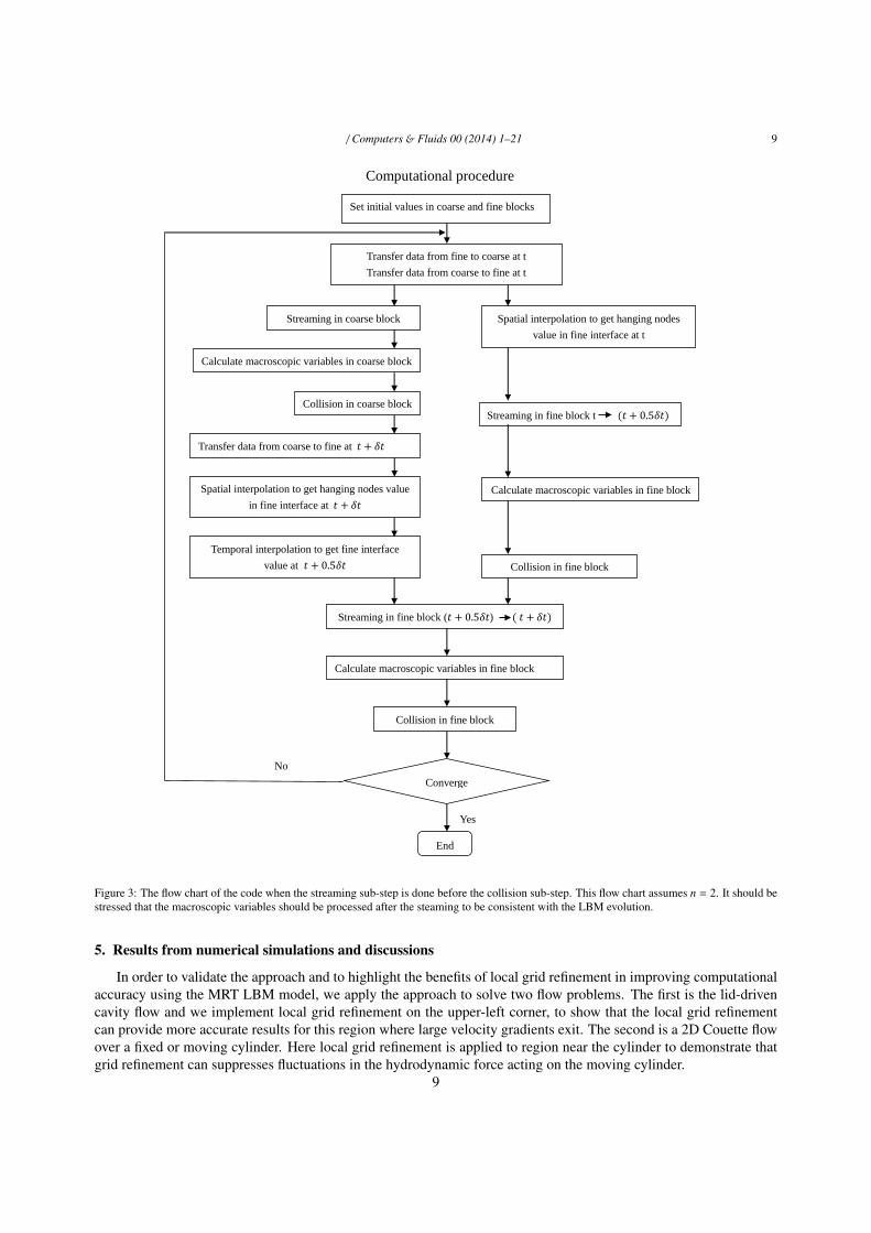
Fig. 3 provides a flow chart for the code when the local refinement is applied to a moving particle, namely, thegrid refinement is done around a moving solid particle, with the fine domain moving with the solid particle. For thischart, it is assumed that the streaming sub-step is performed before the collision sub-step. One can do collision firstthen streaming without changing other process in the flow chart. But data transfer with Eqs. (38) and (40) is replacedby the following relationships, respectively.

f f = M−1 [meq,c + T c (Mfc −meq,c)

], (42)

fc = M−1[meq, f + T f

(Mf f −meq, f

)]. (43)

8


Computational procedure

Converge

End

Transfer data from fine to coarse at t

Transfer data from coarse to fine at t

Streaming in coarse block

Spatial interpolation to get hanging nodes

value in fine interface at t

Calculate macroscopic variables in coarse block

Collision in coarse block

Transfer data from coarse to fine at 𝑡 + 𝛿𝑡

Spatial interpolation to get hanging nodes value

in fine interface at 𝑡 + 𝛿𝑡

Temporal interpolation to get fine interface

value at 𝑡 + 0.5𝛿𝑡

Streaming in fine block t (𝑡 + 0.5𝛿𝑡)

Calculate macroscopic variables in fine block

Collision in fine block

Streaming in fine block (𝑡 + 0.5𝛿𝑡) ( 𝑡 + 𝛿𝑡)

Calculate macroscopic variables in fine block

Collision in fine block

Set initial values in coarse and fine blocks

No

Yes

Figure 3: The flow chart of the code when the streaming sub-step is done before the collision sub-step. This flow chart assumes n = 2. It should bestressed that the macroscopic variables should be processed after the steaming to be consistent with the LBM evolution.

5. Results from numerical simulations and discussions

In order to validate the approach and to highlight the benefits of local grid refinement in improving computationalaccuracy using the MRT LBM model, we apply the approach to solve two flow problems. The first is the lid-drivencavity flow and we implement local grid refinement on the upper-left corner, to show that the local grid refinementcan provide more accurate results for this region where large velocity gradients exit. The second is a 2D Couette flowover a fixed or moving cylinder. Here local grid refinement is applied to region near the cylinder to demonstrate thatgrid refinement can suppresses fluctuations in the hydrodynamic force acting on the moving cylinder.

9


Table 1: Parameters used in the simulations of two dimensional square cavity flow under three different grid configurations.

UCG UCG-L UFG

Uw 0.1 0.10025 0.05H 100 99.75 200ν 0.01 0.01 0.01

Re 1000 1000 1000Nx ∗ Ny 100 ∗ 100 100 ∗ 100 200 ∗ 200

Total node points 10000 12107 40000

5.1. Lid driven cavity flow

The lid-driven cavity flow has been extensively used as a benchmark case to test a numerical method [2, 21]. Inthis flow, the two corners under the moving lid are singular points, and higher grid resolution is desired in order toobtain more accurate stress distribution near the corner points. We apply local grid refinement to the top-left corner(Fig. 4). The simulations are carried out using three different grid configurations: a uniform coarse grid (UCG), auniform coarse grid with local grid refinement (UCG-L) at the top-left corner, and a uniform fine grid (UFG). Thephysical and simulation parameters are listed in Table 1. For all three grid resolutions, the flow Reynolds numberRe = HUw/ν is fixed to 1000, where H is the width of the square cavity, Uw is the lid velocity, and ν is the kinematicviscosity. The bulk viscosity ξ was set to be equal to ν, and these lead to S c

e = 1.8868, S cν = 1.8868 in the coarse

region where δtc = 1 and δxc = 1. The two remaining relaxation parameters in the coarse region are S cε = 1.54 and

S cq = 1.9. For the UCG-L case, a refined grid with dx f = 0.5 is applied to a region near the top-left corner of the size

26 × 26. These lead to the setting that S fe = 0.641, S f

ν = 0.641 , S fε = 1.54,and S f

q = 1.9.

yN

xN

wu

0.26 xN0.26 yN

Figure 4: Local grid refinement block layout for a 2D cavity flow

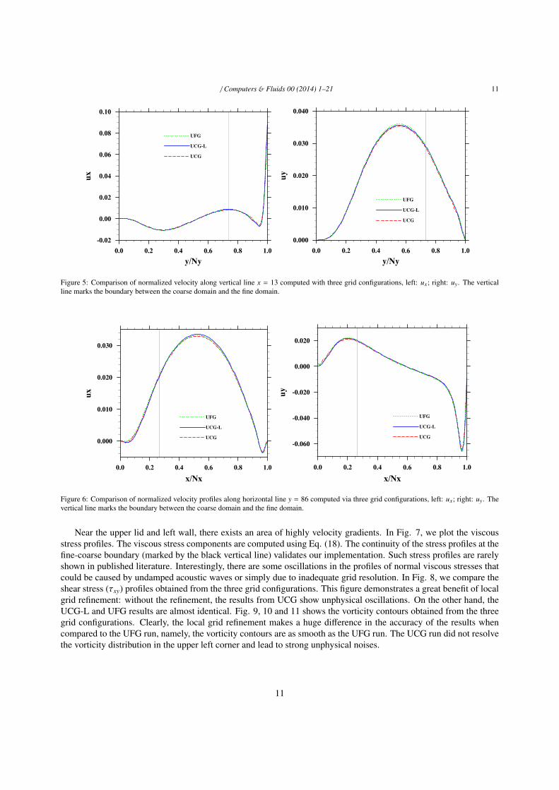
The flow is initially at rest. After a sufficiently long time (over 100,000 coarse-grid time steps), the flow reachesto a steady state. The two velocity components along a vertical line at x = 13 and a horizontal line at y = 86 areshown in Fig. 5 and 6, respectively. Both lines cut though the fine domain. Clearly, the profiles are continuous at thefine-coarse boundary (marked by the vertical line). Second, the results from the three grid configurations essentiallyoverlap, but the UCG-L profiles match better the UFG results, when compared to the UCG results. This shows thatthe local grid refinement improves the results.

10


Figure 5: Comparison of normalized velocity along vertical line x = 13 computed with three grid configurations, left: ux; right: uy. The verticalline marks the boundary between the coarse domain and the fine domain.

Figure 6: Comparison of normalized velocity profiles along horizontal line y = 86 computed via three grid configurations, left: ux; right: uy. Thevertical line marks the boundary between the coarse domain and the fine domain.

Near the upper lid and left wall, there exists an area of highly velocity gradients. In Fig. 7, we plot the viscousstress profiles. The viscous stress components are computed using Eq. (18). The continuity of the stress profiles at thefine-coarse boundary (marked by the black vertical line) validates our implementation. Such stress profiles are rarelyshown in published literature. Interestingly, there are some oscillations in the profiles of normal viscous stresses thatcould be caused by undamped acoustic waves or simply due to inadequate grid resolution. In Fig. 8, we compare theshear stress (τxy) profiles obtained from the three grid configurations. This figure demonstrates a great benefit of localgrid refinement: without the refinement, the results from UCG show unphysical oscillations. On the other hand, theUCG-L and UFG results are almost identical. Fig. 9, 10 and 11 shows the vorticity contours obtained from the threegrid configurations. Clearly, the local grid refinement makes a huge difference in the accuracy of the results whencompared to the UFG run, namely, the vorticity contours are as smooth as the UFG run. The UCG run did not resolvethe vorticity distribution in the upper left corner and lead to strong unphysical noises.

11


Figure 7: Stress profiles computed with local grid refinement , left: along x = 13 ; right: along y = 86. The vertical line marks the boundarybetween the coarse domain and the fine domain.

Figure 8: Comparison of τxy along vertical line x = 13 computed via three grid configurations, left: whole domain view; right: the zoom-in plot.The vertical line marks the boundary between the coarse domain and the fine domain.

12


x

y

0.2 0.4 0.6 0.8 1

0.2

0.4

0.6

0.8

Figure 9: Voticity contours in the cavity: the UCG case.

x

y

0.2 0.4 0.6 0.8 1

0.2

0.4

0.6

0.8

Figure 10: Voticity contours in the cavity: the UCG-L case.

13


Table 2: Computer CPU and memory occupied by three grid structures with cavity flow.

UCG UCG-L UFG

CPU (ms) 5.055 11.416 20.213Memory (kB) 2212 2860 7192

x

y

0.2 0.4 0.6 0.8 1

0.2

0.4

0.6

0.8

Figure 11: Vorticity contours in the cavity: the UFG case.

Finally, in Table 2, we compare the CPU per time step used and memory required for the three cases. While theUFG run uses 4 times CPU and about 3.5 times memory when compared to the UCG run, the UCG-L only uses 2.26times CPU and 29% more memory.

5.2. An asymmetrically placed cylinder in a 2D Couette flow

Next, we consider the same flow studied in [20], namely, an asymmetrically placed cylinder in a 2D Couette flow(Fig. 12). The flow can be simulated in two frames of reference to study the accuracy of moving particle simulation.In the first (or the fixed cylinder case) case, the cylinder particle is fixed relative to the lattice grid and the upper andlower channel boundaries move in opposite direction with a same constant velocity (Ub). In the second case (themoving cylinder case), the cylinder moves at a velocity u0, with the top wall and bottom wall moving at velocityUb1 = Ub + u0 and Ub2 = −Ub + u0, respectively. Physically, the two cases are identical. Numerically, the second caseis much more difficult due to the need to treat the curved moving fluid-cylinder surface. We implemented local gridrefinement in both cases. For the moving cylinder case, the fine domain shifts by one lattice grid every time the centerof the cylinder is moved by one lattice grid.

The geometric parameters for this problem include the channel width Ly and length Lx, the diameter of the cylinderD, and the cylinder center at the initial time (Xc0,Yc0). Periodic boundary condition is used in the x direction, andthe no-slip condition is assumed at the top and bottom channel walls as well as on the cylinder surface. Again, weconsider three grid configurations: uniform coarse grid (UCG), uniform coarse grid with local grid refinement aroundthe cylinder (UCG-F), and uniform fine grid (UFG). The kinematic viscosity is 1/9, which yields S ν = 1.2 in the

14


Table 3: Parameters setting of three grid structures in lattice Boltzmann space.

Parameter UCG UCG-L UFG

Nx × Ny 201 × 101 201 × 101 402 × 202D 25.25 25.25 50.5

(Xc0,Yc0) (30, 54) (30, 54) (60, 108)u0 0.005 0.005 0.0025Ub 0.1 0.1 0.05

coarse domain. Other relaxation parameters in the coarse domain are set to S ε = 1.4 and S e = S q = 1.5 (i.e., thebulk viscosity is 1/18). The other parameters in the moving cylinder simulations are set in Table 3. Note that theparameters for the fixed cylinder case are the same, except u0 = 0. In the fine domain with n = 2, the resultingrelaxation parameters are S f

ν = 6/7, S fe = 1.2, S f

q = 1.5, S fε = 1.4.

Figure 12: Sketch of 2D Couette flow containing a cylinder.

5.2.1. The fixed cylinder case

Figure 13: The hydrodynamic force Fx acting on the fixed cylinder, left: the whole time interval; right: zoom-in plot.

In this case, u0 = 0. The size of the fine domain is a square of size equal to 36. The region covers 12 < x < 48 and36 < y < 72. The no-slip condition on the cylinder surface was handled by a quadratic interpolation scheme [20, 22].Figs. 13, 14 and 15 show the drag force Fx, lift force Fy, and torque as functions of time acting on the particle,

15


respectively. The force and torque are computed by the Galilean invariant momentum exchange method [22, 23].Overall, the results from the three grid configurations are in excellent agreement. The zoom-in plots for 4000 < t <4100 show a very minor difference, typical 0.05% relative difference or less. This is clearly negligible. Therefore,each of these fixed cylinder results can be used as a benchmark to examine results for the moving cylinder case.

5.2.2. Moving particle flow simulationWhen the cylinder is moving at u0, the fine domain is also a squared but with width equal to 32, initially covering

14 < x < 46 and 38 < y < 70. It is more or less placed with the cylinder near the center. Every time the cylindermoves by one lattice unit, the fine domain is shifted in the same direction. When the cylinder moves relative to thegrid, a solid node may become a fluid node and the distribution functions at such new fluid node need to be filled. Therefilling scheme is based on a newly developed velocity-constrained extrapolation scheme [22]. In Figs. 16, 17, 18,we show the drag force Fx, lift force Fy, and torque as functions of time acting on the particle, respectively. Note thatdue to the improved scheme, the level of force fluctuations in Figs. 16 and 17 is significantly less than the level offorce fluctuations shown in Fig. 5 of [20].

The zoom-in view shows that the UCG run has larger magnitude of force fluctuations when compared to that ofthe UFG run. The results from the UCG-L run are more similar to the UFG run than to the UCG run, showing thebenefit of local grid refinement. In order to compare the level of force fluctuations quantitatively, we use the data fromthe fixed cylinder case as the benchmark and compute the L2 norm of the difference as [20],

∆ (t) =

√∑‖F1 (t) − F0 (t)‖2∑‖F0 (t)‖2

(44)

Where F1(t) and F0(t) are the force values of the later part simulated with moving particle and fixed particle, respec-tively. The results are listed in Table 4. The local grid refinement reduces the level of unphysical force fluctuations byroughly a factor of 2.

Figure 14: The hydrodynamic force Fy acting on the fixed cylinder, left: the whole time interval; right: zoom-in plot.

16


Figure 15: The hydrodynamic torque acting on the fixed cylinder, left: the whole time interval; right: zoom-in plot.

Figure 16: The hydrodynamic force Fx acting on the moving cylinder, left: the whole time interval; right: zoom-in plot.

Figure 17: The hydrodynamic force Fy acting on the moving cylinder, left: the whole time interval; right: zoom-in plot.

17


Table 4: L2 error norm for three grid configurations: the moving cylinder case.

Force UCG UCG-L UFG

∆x (t) 0.00151 0.000771 0.000589∆y (t) 0.00942 0.005648 0.002972

Figure 18: The hydrodynamic torque acting on the moving cylinder, left: the whole time interval; right: zoom-in plot.

In Fig.19 we show the normal stress components τxx, τyy and shear stress τxy at the end of the simulation t = 5000.The two inner and two outer vertical lines mark the edge of the cylinder and the fine-coarse boundary, respectively. Ofimportance is that all stress profiles show a consistency at fine-coarse grid interface, namely, both the value and slopeat the fine-coarse boundary are continuous. This again validates our implementation of the local grid refinement.

Figure 19: Stress distribution along y = 51. The thin vertical lines mark the fine-coarse domain boundaries and locations of solid surface.

The CPU time per running step and computer memory requirements are compared in Table 5. We find that thecomputing resources needed for UCG-L run are very similar to UCG, while these for UFG are much larger.

18


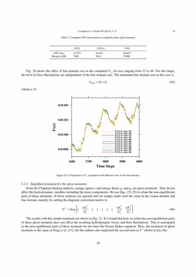
Table 5: Computer CPU and memory occupied by three grid structures

UCG UCG-L UFG

CPU (ms) 19.274 24.432 64.827Memory (kB) 7400 9416 25480

Fig. 20 shows the effect of fine-domain size in the computed Fx, for size ranging from 32 to 48. For this range,the level of force fluctuations are independent of the fine-domain size. The minimum fine-domain size in this case is

S min = D + 6, (45)

which is 31.

Figure 20: Comparison of Fx computed with different sizes of the fine domain.

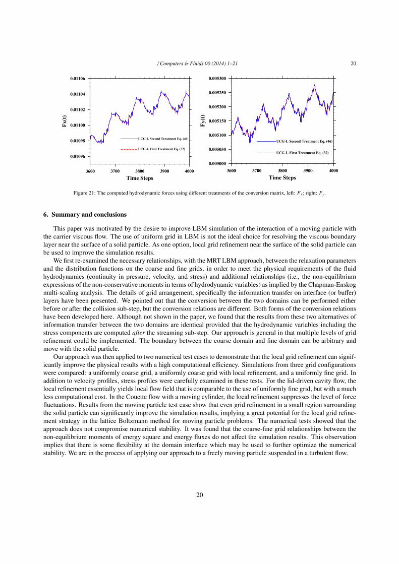
5.2.3. Simplified treatment for the ghost momentsFrom the Chapman-Enskog analysis, energy square ε and energy fluxes qx and qy are ghost moments. They do not

affect the hydrodynamic variables including the stress components. We use Eqs. (23-25) to relate the non-equilibriumparts of these moments. If these relations are ignored and we simply make each the same in the coarse domain andfine domain, namely, by setting the diagonal conversion matrix to

T f = diag[1

nS fe

S ce

1 1 1 1 1nS f

ν

S cν

nS fν

S cν

]. (46)

The results with this simple treatment are shown in Fig. 21. It is found that how we relate the non-equilibrium partsof these ghost moments does not affect the resulting hydrodynamic forces and their fluctuations. This is anticipatedas the non-equilibrium parts of these moments do not enter the Navier-Stokes equation. Here, the treatment of ghostmoments is the same as Peng et al. [17], but the authors also neglected the second term in T f shown in Eq (46).

19


Figure 21: The computed hydrodynamic forces using different treatments of the conversion matrix, left: Fx; right: Fy.

6. Summary and conclusions

This paper was motivated by the desire to improve LBM simulation of the interaction of a moving particle withthe carrier viscous flow. The use of uniform grid in LBM is not the ideal choice for resolving the viscous boundarylayer near the surface of a solid particle. As one option, local grid refinement near the surface of the solid particle canbe used to improve the simulation results.

We first re-examined the necessary relationships, with the MRT LBM approach, between the relaxation parametersand the distribution functions on the coarse and fine grids, in order to meet the physical requirements of the fluidhydrodynamics (continuity in pressure, velocity, and stress) and additional relationships (i.e., the non-equilibriumexpressions of the non-conservative moments in terms of hydrodynamic variables) as implied by the Chapman-Enskogmulti-scaling analysis. The details of grid arrangement, specifically the information transfer on interface (or buffer)layers have been presented. We pointed out that the conversion between the two domains can be performed eitherbefore or after the collision sub-step, but the conversion relations are different. Both forms of the conversion relationshave been developed here. Although not shown in the paper, we found that the results from these two alternatives ofinformation transfer between the two domains are identical provided that the hydrodynamic variables including thestress components are computed after the streaming sub-step. Our approach is general in that multiple levels of gridrefinement could be implemented. The boundary between the coarse domain and fine domain can be arbitrary andmove with the solid particle.

Our approach was then applied to two numerical test cases to demonstrate that the local grid refinement can signif-icantly improve the physical results with a high computational efficiency. Simulations from three grid configurationswere compared: a uniformly coarse grid, a uniformly coarse grid with local refinement, and a uniformly fine grid. Inaddition to velocity profiles, stress profiles were carefully examined in these tests. For the lid-driven cavity flow, thelocal refinement essentially yields local flow field that is comparable to the use of uniformly fine grid, but with a muchless computational cost. In the Couette flow with a moving cylinder, the local refinement suppresses the level of forcefluctuations. Results from the moving particle test case show that even grid refinement in a small region surroundingthe solid particle can significantly improve the simulation results, implying a great potential for the local grid refine-ment strategy in the lattice Boltzmann method for moving particle problems. The numerical tests showed that theapproach does not compromise numerical stability. It was found that the coarse-fine grid relationships between thenon-equilibrium moments of energy square and energy fluxes do not affect the simulation results. This observationimplies that there is some flexibility at the domain interface which may be used to further optimize the numericalstability. We are in the process of applying our approach to a freely moving particle suspended in a turbulent flow.

20


7. Acknowledgements

This work is supported by the National Natural Science Foundation of China (51176102) and granted by ChinaScholarship Council (201308370116). The work is also support by the U.S. National Science Foundation (NSF) undergrants CBET-1235974 and AGS-1139743 and by Air Force Office of Scientific Research under grant FA9550-13-1-0213, LPW also acknowledges support from the Ministry of Education of P.R. China and Huazhong University ofScience and Technology through Chang Jiang Scholar Visiting Professorship.

References

[1] S. Chen and G. Doolen, Lattice Boltzmann method for fluid flows, Annu. Rev. Fluid Mech. 30 (1998) 329-364.[2] D. Yu, R. Mei, L.-S. Luo, W. Shyy, Viscous flow computations with the method of lattice Boltzmann equation, Progr. Aerospace Sci.39

(2003) 329-367.[3] D. Raabe, Overview of the lattice Boltzmann method for nano- and microscale fluid dynamics in materials science and engineering, Model.

Simul. Mater. Sci. Eng. 12 (2004) R13-R46.[4] S. Succi, The Lattice Boltzmann Equation for Fluid Dynamics and Beyond, Clarendon Press, Oxford, 2001.[5] P. L. Bhatnagar, E. P. Gross, M. Krook, A model for collision processes in gases. I. Small amplitude processes in charged and neutral

one-component system, Physical Review 94 (1954) 511-525.[6] P. Lallemand and L.-S. Luo, Theory of the lattice Boltzmann method: Dispersion, dissipation, isotropy, Galilean invariance, and stability,

Phys. Rev. E 61 (2000) 6546.[7] D. Humieres, I. Ginzburg, M. Krafczyk, P. Lallemand, L.-S. Luo, Multiple relaxation-time lattice Boltzmann models in three dimensions,

Philos. Trans. R. Soc. London A 360 (2002) 437-451.[8] R. Mei, L.-S. Luo, P. Lallemand, D. d’Humieres, Consistent initial conditions for lattice Boltzmann simulation, Computer & Fluids, 35 (2006)

855-862.[9] O. Filippova and D. Hanel, Grid refinement for lattice-BGK models, J. Comput. Phys. 147 (1998) 219-228.

[10] O. Filippova and D. Hanel, Acceleration of lattice-BGK schemes with grid refinement, J. Comput. Phys. 165 (2000) 407-427.[11] D. Yu, R. Mei, W. Shyy, A multi-block lattice Boltzmann method for viscous fluid flows, Int. J. Numer. Methods Fluids 39 (2002) 99-120.[12] D. Yu and S. S. Girimaji, Multi-block Lattice Boltzmann method: Extension to 3D and validation in turbulence, Physica A 362 (2006)

118-124.[13] G. Eitel-Amor, M. Meinke, W. Schroder, A lattice-Boltzmann method with hierarchically refined meshes, Computers and Fluids 75 (2013)

127-139.[14] D. Lagrava, O. Malaspinas, J. Latt , B. Chopard. Advances in multi-domain lattice Boltzmann grid refinement, Journal of Computational

Physics 231 (2012) 4808-4882.[15] M. Dietzel and M. Sommerfeld, Numerical calculation of flow resistance for agglomerates with different morphology by the LatticeBoltzmann

Method, Powder Technology, 250 (2013) 122-137.[16] K. N. Premnath, M. J. Pattison, S. Banerjee, An Investigation of the Lattice Boltzmann Method for Large Eddy Simulation of complex

Turbulent Separated Flow, Journal of Fluids Engineering 135 (2013) 051401-051412.[17] Y. Peng, C. Shu, Y. T. Chew, X. D. Niu, X. Y. Lu, Application of multi-block approach in the immersed boundary lattice Boltzmann method

for viscous fluid flows, J. Comput. Phys. 218 (2006) 460-478.[18] B. Chopard, M. Droz, Cellular Automata Modeling of Physical Systems, Cambridge University Press, 1998.[19] X. Shan, X. F. Yuan, H. Chen, Kinetic theory representation of hydrodynamics: a way beyond the Navier-Stokes equation, J. Fluid Mech.

550 (2006) 413-441.[20] P. Lallemand, L. S. Luo, Lattice Boltzmann method for moving boundaries, J. Comput. Phys. 184 (2003) 406-421.[21] U. Ghia, K. N. Ghia, C. T. Shin, High resolution for incompressible flow using the Navier-Stokes equations and a multi-grid method, J.

Comput. Phys. 48 (1982) 387-411.[22] C. Peng, Y. Teng, B. Hwang, Z. Guo, L.-P. Wang, Implementation issues and benchmarking of moving particle simulations in a viscous flow,

submitted to the ICMMES2014 special issue.[23] B. Wen, C. Zhang, Y. Yu, et al, Galilean invariant fluid-solid interfacial dynamics in lattice Boltzmann simulations, J Comp. Phys. 266 (2014)

161-170.

21

computers & fluids improving lattice boltzmann simulation...

Documents