LARGE SCALE LANDSLIDE SUSCEPTIBILITY ASSESSMENT USING 1 

THE STATISTICAL METHODS OF LOGISTIC REGRESSION AND 2 

BSA. STUDY CASE: THE SUB-BASIN OF THE SMALL NIRAJ 3 

(TRANSYLVANIA DEPRESSION, ROMANIA) 4 

5 

Sanda, Roșca1, Ştefan, Bilaşco1,2, Dănuţ, Petrea1, Ioan Fodorean1 , Iuliu Vescan1 , Sorin 6 

Filip 1 & Flavia–Luana Măguț1 7 

1"Babeş-Bolyai" University, Faculty of Geography, 400006 Cluj-Napoca, Romania, 8 rosca_sanda@yahoo.com, sbilasco@geografie.ubbcluj.ro dpetrea@geografie.ubbcluj.ro, 9 fioan@geografie.ubbcuj.ro, vescan@geografie.ubbcluj.ro, sfilip@geografie.ubbcluj.ro, 10 luana.magut@gmail.com 11 2Romanian Academy, Cluj-Napoca Subsidiary Geography Section, 9, Republicii Street, 400015, Cluj-12 Napoca, Romania 13 Correspondence to: Sanda, ROȘCA (rosca_sanda@yahoo.com) 14 

15 ABSTRACT: The existence of a large number of GIS models for the identification of landslide 16 occurrence probability makes difficult the selection of a specific one. The present study focuses 17 on the application of two quantitative models: the logistic and the BSA models. The comparative 18 analysis of the results aims at identifying the most suitable model. The territory corresponding 19 to the Niraj Mic Basin (87 km2) is an area characterised by a wide variety of the landforms with 20 their morphometric, morphographical and geological characteristics as well as by a high 21 complexity of the land use types where active landslides exist. This is the reason why it 22 represents the test area for applying the two models and for the comparison of the results. The 23 large complexity of input variables is illustrated by 16 factors which were represented as 72 24 dummy variables, analysed on the basis of their importance within the model structures. The 25 testing of the statistical significance corresponding to each variable reduced the number of 26 dummy variables to 12 which were considered significant for the test area within the logistic 27 model, whereas for the BSA model all the variables were employed. The predictability degree 28 of the models was tested through the identification of the area under the ROC curve which 29 indicated a good accuracy (AUROC = 0.86 for the testing area) and predictability of the logistic 30 model (AUROC = 0.63 for the validation area). 31 

32 Keywords: Landslide modelling, Logistic regression, BSA, GIS database, GIS modelling, 33 comparation 34  35 

1. GENERAL CONSIDERATION 36  37 One of the main natural hazards affecting the territory of Romania is represented by landslides 38 

which have a high spatial and temporal frequency and cause damages to transport infrastructure and 39 

buildings and determine environmental changes (Bălteanu and Micu 2009; Bilașco et. al 2011; Năsui 40 

and Petreuș 2014). 41 

EEA European Directive from 2004 underlines the need to mapping and identification areas with 42 

vulnerability to landslides using indirect techniques in European and national context (Guzetti 2006; Van 43 

Westen et al. 2006; Magliulio et al. 2008; Polemio and Petruci 2010). 44 

Thus, the studies determining their probability of occurrence are highly valuable in the process 45 

of reducing their potential negative effects. Among the methods used for determining the spatial 46 

probability of landslides, statistical methods are recommended by very good results and high validation 1 

rates (Zezere et al 2004; Petrea et al. 2014; Roșca et al. 2015a,b). 2 

Considering the increase in the number of possibilities for data processing and the evolution of 3 

methods developed in the GIS environment, various methods of landslide susceptibility assessment 4 

have been developed, out of which the logistic regression and bivariate statistical analysis methods is 5 

one of the most frequently used (Harrell 2001; Kleinbaum and Klein 2002; Ayalew and Yamagishi 2004; 6 

Dai and Lee 2002; Ayalew and Yamagishi 2005; Lee 2005; Cuesta et al. 2010; Chiţu 2010; Mancini et 7 

al. 2010; Wang et al. 2011; Guns and Vanacker 2012; Jurchescu 2013; Măguţ et al. 2013, Akbari et al. 8 

2014; Van den Eeckhaut et al. 2010). This analysis starts from the hypothesis that the combination of 9 

factors which led to the occurrence of landslides in the past will have the same effect in the future 10 

(Crozier and Glade 2005). 11 

Among the advantages of this method one must take into consideration the possibility of simultaneously 12 

integrating both quantitative and qualitative data in the model and the testing of v represent dependent 13 

variables while their triggering and preparing factors are the independent (explanatory) variables. 14 

The purpose of this study is to identify the large scale susceptibility of landslide occurrence by 15 

applying the logistic model in the sub-basin of the Small Niraj (Fig. 1). The database included a complete 16 

landslide inventory and the descriptive data of 16 causing factors used for generating the model. These 17 

factors describe the morphometrical, geological and the hydroclimatic characteristics of the territory 18 

under analysis. 19 

Fig. 1: Geomorphological map of the Small Niraj catchment and geographical position of the study area 20 (1 – flood plain, 2 – slopes and connecting surfaces, 3 – slopes with complex modellation, 4 – active 21 landslides, 5 – permanent hydrographic network, 6 – temporary hydrographic network, 7 – watershed 22 divide, 8 – settlements) 23  24 

2. STUDY AREA 25 

The study area is located in the north-east of Transylvania Depression, Romania, and has 26 

recorded important economical and environmental losses over in the last two years: 67 persons, 45 27 

houses, 115 hectares of land and a country road were affected by landslides. The catchment area is 28 

found between 24°47΄52" and 24°58΄32" eastern longitude and 46°30΄53" and 46°37΄42" northern 29 

latitude, totalizing an area of 68 km2 and including the territories of ten settlements. The Small Niraj 30 

represents the main river of the area. 31 

Based on the Romanian National Meteorological Administration Institute the mean temperature 32 

varies between – 4.2° C in January and 17.9° C in August. The mean annual rainfall is around 622 1 

mm/year, while the maximum precipitation falls between May (73.5 mm) and June (81.5 mm). 2 

3. DATABASE AND METHODOLOGY 3 

GIS spatial analysis models are built upon complex structures and databases generated from 4 

varied sources. One of the main problems to solve during the building of a spatial analysis model that 5 

localizes the areas with different landslide susceptibility values is represented by the identification of its 6 

actual format along with the building and the integrated management of the model input data. 7 

The large variety of databases serving as input data in the complex identification model 8 

concerning landslide susceptibility, makes it that the different model structures have a resolution 9 

dependent on the model scale. Bearing in mind that the scale for the models fits within the large scale 10 

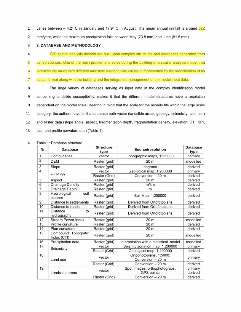
category, the authors have built a database both vector (landslide areas, geology, seismicity, land use) 11 

and raster data (slope angle, aspect, fragmentation depth, fragmentation density, elevation, CTI, SPI, 12 

plan and profile curvature etc.) (Table 1). 13 

Table 1: Database structure 14 

Nr. Database Structure

type Source/resolution

Database type

1. Contour lines vector Topographic maps, 1:25.000 primary 2. DEM Raster (grid) 20 m modelled

3. Slope Raster (grid) degrees derived 4.

Lithology vector Geological map, 1:200000 primary

Raster (Grid) Conversion – 20 m derived 5. Aspect Raster (grid) 20 m derived 6. Drainage Density Raster (grid) m/km derived 7. Drainage Depth Raster (grid) m derived 8. Hydrological soil

classes Raster (grid) Soil Map, 1:200000 derived

9. Distance to settlements Raster (grid) Derived from Ortofotoplans derived 10 Distance to roads Raster (grid) Derived from Ortofotoplans derived 11. Distance to

hydrography Raster (grid) Derived from Ortofotoplans derived

12. Stream Power Index Raster (grid) 20 m modelled 13. Profile curvature Raster (grid) 20 m derived 14. Plan curvature Raster (grid) 20 m derived 15. Compound Topografic

Index (CTI) Raster (grid) 20 m modelled

16. Precipitation data Raster (grid) Interpolation with a statistical model modelled 17.

Seismicity vector Seismic zonation map, 1:200000 primary

Raster (Grid) Geological map, 1:200000 derived 18.

Land use vector

Ortophotoplans, 1:5000; Conversion – 20 m

primary

Raster (Grid) Conversion – 20 m derived 19.

Landslide areas vector

Spot Images, orthophotograps, GPS points

primary derived

Raster (Grid) Conversion – 20 m derived

20. Landslide probability map

Raster (Grid) Equations of spatial analysis

(20 m resolution) modelled

1 

The spatial distribution of the 16 factors included in the model was determined using GIS 2 

functions of spatial analysis included in the ArcGis software. 3 

The different database sources made their validation mandatory so as to ensure an accurate 4 

representation. The validation of the databases was done using the comparison technique (the database 5 

was compared to field data) as well as using observation (by visual identification of the correspondence 6 

existing between the cartographic representation and the existing situation in the field). Having the 7 

certainty that a valid and accurate database is used, the logical schemas of the BSA and logistic model 8 

were subsequently completed in order to be used for determining the probability of landslide occurrence. 9 

The landslide susceptible areas are identified through the BSA model by considering the statistic 10 

value specific to each class of the factors included in the initial database, without taking into account the 11 

importance of the factor within the informational flux of the model. The statistical model based on the 12 

bivariate probability analysis was applied to predict the spatial distribution of landslides by estimating 13 

the probability of landslide occurrence based on the assumption that the prediction should start from the 14 

existing landslides: Chung et al. 1995; Dhakal et al. 2000; Saha 2002; Sarkar and Kanungo 2004; 15 

Magiulio et al. 2008; etc. 16 

The statistical value of each factor class included in the bivariate model was calculated using 17 

the equation proposed by Yin and Yan, 1988, as well as Jade and Sarkar 1993: 18 

, (1) 19 

where: 20 Ii = Statistical value of the analysed factor 21 Si = Area affected by landslides for the analysed variable 22 Ni = Area of the analysed variable 23 S = Total landslide area in the analysed basin 24 N = Area of the analysed basin 25  26 By using formula (1), the statistical value of each variable is identified, the insignificant variables 27 

(characterised by negative values) being integrated with an equal weight in the model structure, 28 

occasionally reducing the susceptibility class values. 29 

In order to predict landslide susceptibility at pixel level in the study area the model of logistic 30 

regression was also taken into consideration. This method was mathematically described by Harrel 31 

2001: Ώ represents the set of points (pixels from the study area); Y represents the binary variables (0 32 

for pixels without landslides and 1 for pixels with landslides); X1, ….Xn represent independent variables, 33 

in this study the 15 factors included in the model, each classified in various categories and representhed 1 

with the help of dummy variables, out of which one class was not included in the model in order to be 2 

used as a control value (Van den Eeckhaut et al. 2006). 3 

Thus, the probability of occurrence for a new landslide event is represented by: 4 

, (2) 5 

6 where: 7  Z = β0 + β1X1 + … + βnXn, 8  X1...Xn – preparing and triggering factors 9  β0 – constant , 10 β1... βn - multiplication coefficients. 11  12 One can notice that the probability of occurrence becomes a linear function for each variable included 13 

in the model (Kleimbaum and Klein 2002). In order to estimate the parameters, a logarithmic 14 

transformation of the odds ratio was necessary (represented by the ratio of the probability of success 15 

and the probability of failure) which changes the variation interval from (0,1) to a sigmoid curve, in the 16 

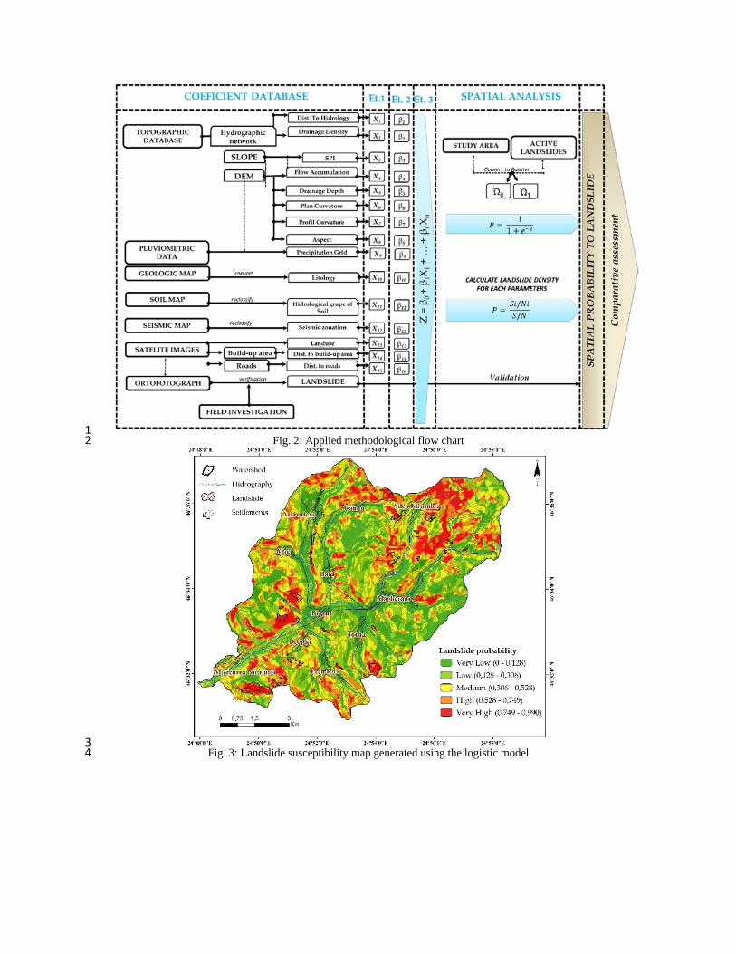
interval (-∞, +∞) (Thiery 2007, cited by Jurchescu 2013). The main methodological stages are described 17 

in Fig. 2. 18 

Fig. 2: Applied methodological flow chart 19 

The Ώ study area was divided into two random sub-categories: Ώ1 and Ώ0. Hence, 500 points 20 

were used in the modelling process, 250 points generated at a minimum distance of 60 metres in the 21 

landslide areas and 250 points at a minimum distance of 80 meters in the non-landslide areas. A number 22 

of 40 landslides were randomly selected for the training stage and 15 landslides were included for the 23 

validation of the model. The validation set of points included a total of 200 randomly generated points 24 

at a minimum distance of 40 meters (100 points inside the landslides and 100 points outside them). The 25 

importance of this stage which relies on a division of the study area in two sets of samples has been 26 

repeatedly emphasised by numerous authors with respect to the independence of the validation set of 27 

data used to test the results of the logistic regression for landslide susceptibility assessment (Van den 28 

Eeckaut et al. 2006; 2010; Mancini et al. 2010, Mărgărint et al. 2013, etc). 29 

The coefficient values (X1, …Xn) of each landslide factor were necessary in order to determine 30 

the probability of landslide occurence for each pixel, these coefficients being considered as 31 

representative for Ώ1 and Ώ0. In order to preserve the independence of the input factors, the 16 variables 32 

were transformed into dummy variables, resulting in a total of 73 variables, as each input factor was 33 

classified in different categories necessary for the comparative analysis. For each factor, one of the 1 

dummy variable was kept for reference (Hilbe 2009). 2 

The multiplication coefficient of each variable was determined by applying the logistic regression 3 

(Table 2). The β0 …βn parameters were estimated using the maximum likelihood ratio (i.e. inverse 4 

probability) (Harrel 2011). This stage identifies the difference between the model which does not include 5 

the X1 parameter in the input database and the model which includes in its input database the Xn 6 

parameter. The variables with the highest influence were identified with the help of the AIC criterium 7 

which indicates the statistical significance of the variable. 8 

A value below 0.05 is considered optimal, representing the threshold for the data acceptable within the 9 

model database. A statistical threshold value of <0.1 determines the elimination of that specific variable 10 

from the present database, as it would raise multicollinearity issues (Cuesta et al. 2010). The coefficients 11 

resulting from the logistic regression were implemented in a GIS environment using the Raster 12 

Calculator functions, by multiplying them with the raster variables which represent the landslide 13 

preparing and triggering factors. 14 

The goodness of fit was determined by generating the area under the ROC curve using the 15 

training data, while the prediction capacity of the model was identified using the validation data set 16 

(Hosmer and Lemeshow 2000; Guzzetti 2006). The quality of the information included in the input 17 

variables for the landslide susceptibility model as well as the number of variables need to be considered 18 

in the process of variable selection, in order to reduce redundancy (Chiţu 2010). 19 

The 16 variables (elevation, slope angle, average precipitation, slope aspect, drainage density, 20 

drainage depth, hydrological soil classes, distance to streams, distance to roads and settlements, 21 

Stream Power Index (SPI), land use, lithology, plan curvature and profile curvature, Topographic 22 

Wetness Index (CTI) were included in the model, their selection being performed according to their 23 

statistical relevance in the logistic regression. 24 

4. RESULTS, VALIDATION AND DISCUSSION 25 

The establishing of the research methodology applied in the present study needs a comparative 26 

approach of the methods and of the results obtained through the implementing of the previously 27 

mentioned models. 28 

The comparison of the spatial analysis methods integrated within the two models emphasises 29 

the difference among the necessary databases, as well as the complexity and implementation possibility 30 

of the models. The comparative approach of the results on the different levels of the modelling process 1 

as well as of the final results shows the practical utility of such databases within each model, as well as 2 

the accuracy of the representation. 3 

4.1. Applied logistic regression to landslide susceptibility assessment 4 

The statistical correlation between the mapped landslides from the Niraj river basin and their causing 5 

factors was determined for the logistic model using the statistical software R. The training variables were 6 

included in the logistic regression and the AIC was used to perform an automated stepwise selection of 7 

the best model, namely the combination of variables which best explains the occurrence of landslides 8 

in the analysed territory. 9 

The model with the best AIC value (AIC = 524) is given by the following expression: 10  11 fit3 = glm(alunec ~ lndse_8 + spi_1 + dst_h5 + as_10 + as_7 + dst_dr6 + lndse_3 + dns_f4 + 12 

as_6 + slop_4 + pp_2 + dst_dr7 + dst_lc7, family = binomial, data = model_df2) 13 (3) 14 

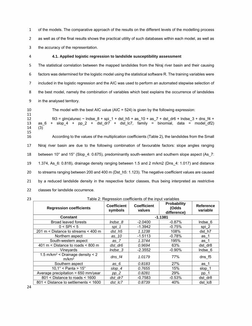
15 According to the values of the multiplication coefficients (Table 2), the landslides from the Small 16 

Niraj river basin are due to the following combination of favourable factors: slope angles ranging 17 

between 10° and 15° (Slop_4: 0.675), predominantly south-western and southern slope aspect (As_7: 18 

1.374, As_6: 0.818), drainage density ranging between 1.5 and 2 m/km2 (Dns_4: 1.017) and distance 19 

to streams ranging between 200 and 400 m (Dst_h5: 1.123). The negative coefficient values are caused 20 

by a reduced landslide density in the respective factor classes, thus being interpreted as restrictive 21 

classes for landslide occurrence. 22 

Table 2: Regression coefficients of the input variables 23 

Regression coefficients Coefficient symbols

Coefficient values

Probability (Odds

difference)

Reference variable

Constant -1.1381 Broad leaved forests lndse_8 -2.0400 -0.87% lndse_6

0 < SPI < 5 spi_1 -1.3942 -0.75% spi_2 201 m < Distance to streams < 400 m dst_h5 1.1238 108% dst_h7

Northern aspect as_10 -1.5113 -0.78% as_1 South-western aspect as_7 1.3744 195% as_1

401 m < Distance to roads < 800 m dst_dr6 0.9694 63% dst_dr8 Vineyards lndse_3 -2.3552 -0.90% lndse_6

1.5 m/km2 < Drainage density < 2 m/km2

dns_f4 1.0179 77% dns_f5

Southern aspect as_6 0.8183 27% as_1 10,1° < Panta > 15° slop_4 0.7655 15% slop_1

Average precipitation = 650 mm/year pp_2 0.8281 29% pp_1801 < Distance to roads < 1600 dst_dr7 -0.7583 -0.53% dst_dr8

801 < Distance to settlements < 1600 dst_lc7 0.8739 40% dst_lc8 24 

For the interpretation of the results, the odds difference plays a very important role (Table 2). 1 

For example, keeping all the input variables constant while the average precipitation value is set at 650 2 

mm/year, the probability of landslide occurrence is by 29% higher than in the case of the reference value 3 

of precipitation (525 mm). 4 

Thus, the highest increase in probability for landslide occurrence is recorded when comparing 5 

the south-western slopes with the reference class of level areas (195%) indicating a powerful 6 

dependency relationship between landslide occurrence and south-western slopes. 7 

The resulting coefficients were multiplied with their corresponding 13 raster files using Raster 8 

Calculator according to formula (4): 9 

Mdl_fit3 = exp(-1.1381 + -2.0400 * [lndse_8] + -1.3942 * [spi_1] + 1.1238 * [dst_h5] + -1.5113 * 10 [as_10] + 1.3744 * [as_7] + 0.9694 * [dst_dr6] + -2.3552 * [lndse_3] + 1.0179 * [dns_f4] + 0.8183 * [as_6] 11 + 0.7655 * [slop_4] + 0.8281 * [pp_2] + -0.7583 * [dst_dr7] + 0.8739 * [dst_lc7]) 12 (4) 13 

14 The landslide susceptibility map was generated by applying the odds ratio formula (5) 15 

representing the landslide susceptibility in the interval 0 – 1 (Fig. 3). 16 

S = p/(1-p), (5) 17 where S - susceptibility, P – probability 18  19 

Fig. 3: Landslide susceptibility map generated using the logistic model 20  21 

The goodness of fit and the predictability of the model were determined using the ROC curve for the 22 

model sample and the testing sample, respectively. The sensitivity of the model represents the true 23 

positive rate (pixels with a high probability of landslide occurrence being validated by real landslides), 24 

while the model specificity represents the probability that the areas identified as highly susceptible to 25 

landslides to be invalidated by the lack of any landslides (false positive rate) (Hosmer and Lemeshow 26 

2000). 27 

Fig. 4: Area under the ROC curve for the training data (left) and the testing data (right) 28  29 

Table 3: Spatial distribution of susceptibility classes 30 

Susceptibility class Statistical value

Area (km2) %

1. Very low 0 – 0.128 21.489 24.70 2. Low 0.128 – 0.306 23.116 26.57 3. Medium 0.306 – 0.528 19.594 22.52 4. High 0.528 – 0.749 13.26 15.24 5. Very high 0.749 – 0.990 9.528 10.95

The area under the ROC (Relative Operational Curve) is 0.86 for the training data set and 0.63 for the 31 

testing (validation) data set, the first value indicating the goodness of model fit while the second 32 

represents the predictability of the model, or its capacity to predict future events (Fig. 4). 33 

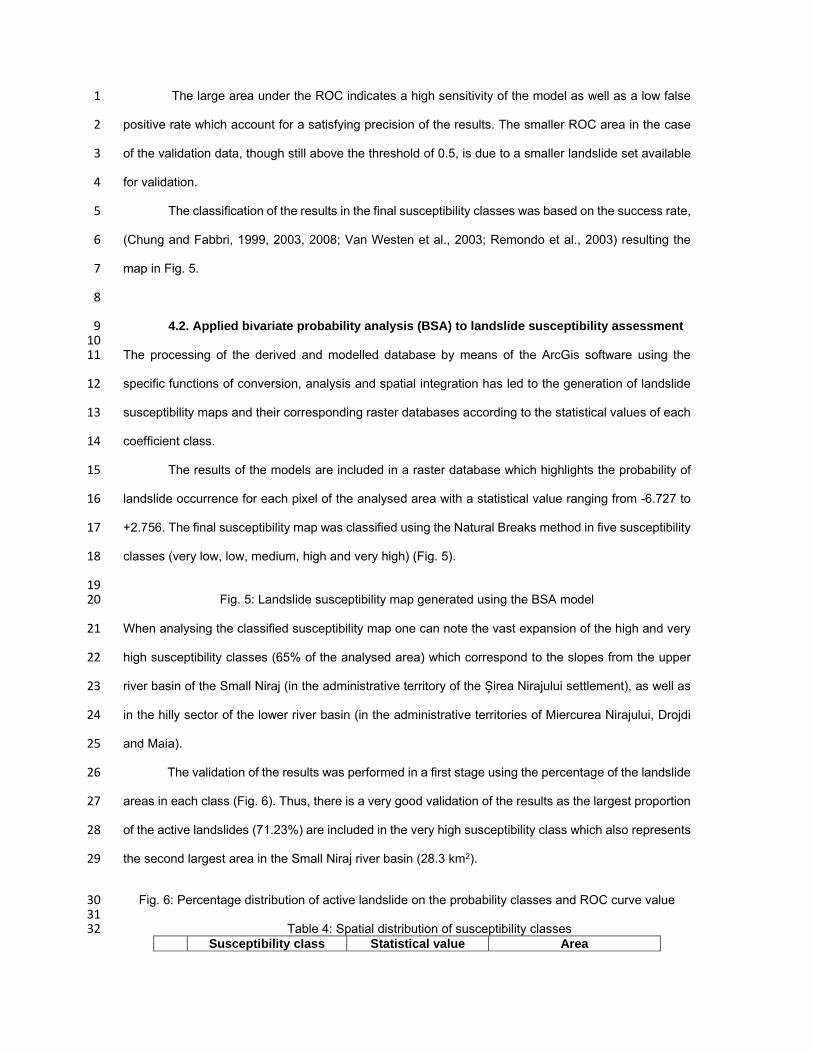
The large area under the ROC indicates a high sensitivity of the model as well as a low false 1 

positive rate which account for a satisfying precision of the results. The smaller ROC area in the case 2 

of the validation data, though still above the threshold of 0.5, is due to a smaller landslide set available 3 

for validation. 4 

The classification of the results in the final susceptibility classes was based on the success rate, 5 

(Chung and Fabbri, 1999, 2003, 2008; Van Westen et al., 2003; Remondo et al., 2003) resulting the 6 

map in Fig. 5. 7 

8 

4.2. Applied bivariate probability analysis (BSA) to landslide susceptibility assessment 9  10 The processing of the derived and modelled database by means of the ArcGis software using the 11 

specific functions of conversion, analysis and spatial integration has led to the generation of landslide 12 

susceptibility maps and their corresponding raster databases according to the statistical values of each 13 

coefficient class. 14 

The results of the models are included in a raster database which highlights the probability of 15 

landslide occurrence for each pixel of the analysed area with a statistical value ranging from -6.727 to 16 

+2.756. The final susceptibility map was classified using the Natural Breaks method in five susceptibility 17 

classes (very low, low, medium, high and very high) (Fig. 5). 18 

19 Fig. 5: Landslide susceptibility map generated using the BSA model 20 

When analysing the classified susceptibility map one can note the vast expansion of the high and very 21 

high susceptibility classes (65% of the analysed area) which correspond to the slopes from the upper 22 

river basin of the Small Niraj (in the administrative territory of the Șirea Nirajului settlement), as well as 23 

in the hilly sector of the lower river basin (in the administrative territories of Miercurea Nirajului, Drojdi 24 

and Maia). 25 

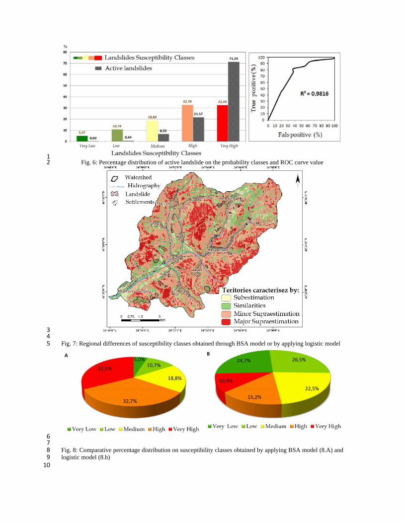
The validation of the results was performed in a first stage using the percentage of the landslide 26 

areas in each class (Fig. 6). Thus, there is a very good validation of the results as the largest proportion 27 

of the active landslides (71.23%) are included in the very high susceptibility class which also represents 28 

the second largest area in the Small Niraj river basin (28.3 km2). 29 

Fig. 6: Percentage distribution of active landslide on the probability classes and ROC curve value 30  31 

Table 4: Spatial distribution of susceptibility classes 32  Susceptibility class Statistical value Area

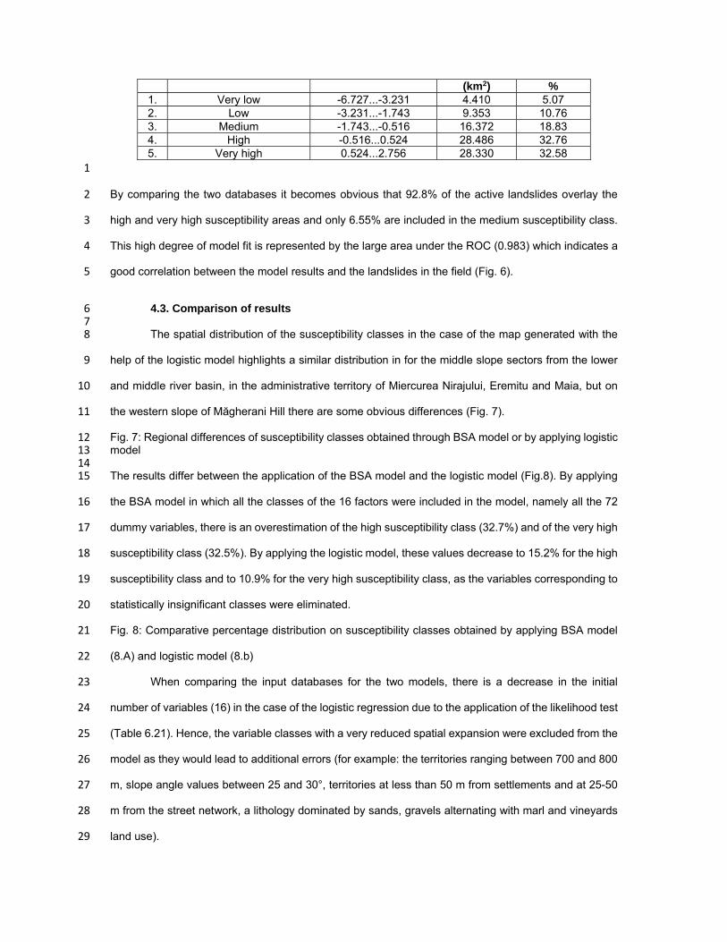
(km2) % 1. Very low -6.727...-3.231 4.410 5.07 2. Low -3.231...-1.743 9.353 10.76 3. Medium -1.743...-0.516 16.372 18.83 4. High -0.516...0.524 28.486 32.76 5. Very high 0.524...2.756 28.330 32.58 1 

By comparing the two databases it becomes obvious that 92.8% of the active landslides overlay the 2 

high and very high susceptibility areas and only 6.55% are included in the medium susceptibility class. 3 

This high degree of model fit is represented by the large area under the ROC (0.983) which indicates a 4 

good correlation between the model results and the landslides in the field (Fig. 6). 5 

4.3. Comparison of results 6  7 The spatial distribution of the susceptibility classes in the case of the map generated with the 8 

help of the logistic model highlights a similar distribution in for the middle slope sectors from the lower 9 

and middle river basin, in the administrative territory of Miercurea Nirajului, Eremitu and Maia, but on 10 

the western slope of Măgherani Hill there are some obvious differences (Fig. 7). 11 

Fig. 7: Regional differences of susceptibility classes obtained through BSA model or by applying logistic 12 model 13  14 The results differ between the application of the BSA model and the logistic model (Fig.8). By applying 15 

the BSA model in which all the classes of the 16 factors were included in the model, namely all the 72 16 

dummy variables, there is an overestimation of the high susceptibility class (32.7%) and of the very high 17 

susceptibility class (32.5%). By applying the logistic model, these values decrease to 15.2% for the high 18 

susceptibility class and to 10.9% for the very high susceptibility class, as the variables corresponding to 19 

statistically insignificant classes were eliminated. 20 

Fig. 8: Comparative percentage distribution on susceptibility classes obtained by applying BSA model 21 

(8.A) and logistic model (8.b) 22 

When comparing the input databases for the two models, there is a decrease in the initial 23 

number of variables (16) in the case of the logistic regression due to the application of the likelihood test 24 

(Table 6.21). Hence, the variable classes with a very reduced spatial expansion were excluded from the 25 

model as they would lead to additional errors (for example: the territories ranging between 700 and 800 26 

m, slope angle values between 25 and 30°, territories at less than 50 m from settlements and at 25-50 27 

m from the street network, a lithology dominated by sands, gravels alternating with marl and vineyards 28 

land use). 29 

Another series of variable classes were excluded from the analysis, for example the territories 1 

with a drainage density between 0.5-1 m/km2, a drainage depth between 51-100 m, the territories 2 

situated at 25-50 m from streams, pastures as well as the slopes with positive values of the plan 3 

curvature due to their low statistical significance. 4 

5 

6 

7 

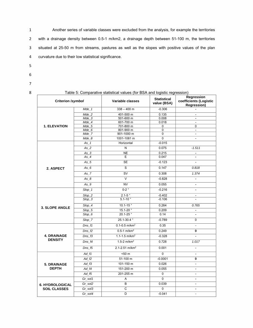
Table 5: Comparative statistical values (for BSA and logistic regression) 8 

Criterion /symbol Variable classes Statistical

value (BSA)

Regression coefficients (Logistic

Regression)

1. ELEVATION

Mde_1 338 – 400 m -0.306 -

Mde_2 401-500 m 0.135 - Mde_3 501-600 m 0.008 - Mde_4 601-700 m 0.018 - Mde_5 701-800 m 0 0 Mde_6 801-900 m 0 - Mde_7 901-1000 m 0 -

Mde_8 1001-1081 m 0 -

2. ASPECT

As_1 Horizontal -0.015

As_2 N 0.075 -1.511

As_3 NE 0.215 - As_4 E 0.047 -

As_5 SE -0.123 -

As_6 S 0.147 0.818

As_7 SV 0.308 1.374

As_8 V -0.828 -

As_9 NV 0.055 -

3. SLOPE ANGLE

Slop_1 0-2 ° -0.216 -

Slop_2 2.1-5 ° -0.402 - Slop_3 5.1-10 ° -0.106 -

Slop_4 10.1-15 ° 0.264 0.765

Slop_5 15.1-20 ° 0.209 - Slop_6 20.1-25 ° 0.14 -

Slop_7 25.1-30.4 ° -0.789 0

4. DRAINAGE DENSITY

Dns_f1 0.1-0.5 m/km2 0.35 -

Dns_f2 0.5-1 m/km2 0.249 0

Dns_f3 1.1-1.5 m/km2 -0.328 -

Dns_f4 1.5-2 m/km2 0.728 1.017

Dns_f5 2.1-2.51 m/km2 0.001 -

5. DRAINAGE

DEPTH

Ad_f1 <50 m 0 -

Ad_f2 51-100 m -0.0001 0

Ad_f3 101-150 m 0.026 -

Ad_f4 151-200 m 0.055 -

Ad_f5 201-255 m 0 -

6. HYDROLOGICAL SOIL CLASSES

Gr_sol1 A 0 -

Gr_sol2 B 0.039 -

Gr_sol3 C 0 -

Gr_sol4 D -0.041 -

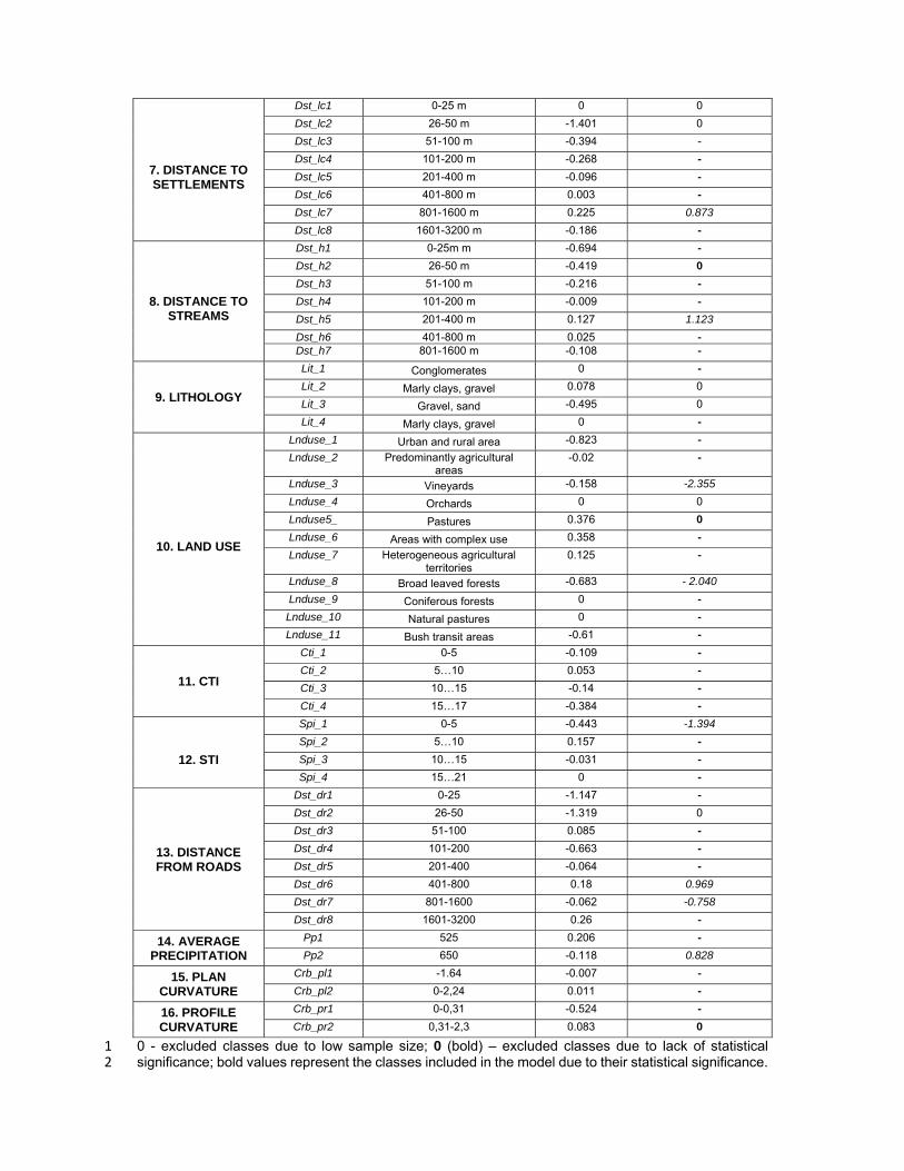
7. DISTANCE TO SETTLEMENTS

Dst_lc1 0-25 m 0 0

Dst_lc2 26-50 m -1.401 0

Dst_lc3 51-100 m -0.394 -

Dst_lc4 101-200 m -0.268 -

Dst_lc5 201-400 m -0.096 -

Dst_lc6 401-800 m 0.003 -

Dst_lc7 801-1600 m 0.225 0.873

Dst_lc8 1601-3200 m -0.186 -

8. DISTANCE TO

STREAMS

Dst_h1 0-25m m -0.694 -

Dst_h2 26-50 m -0.419 0

Dst_h3 51-100 m -0.216 -

Dst_h4 101-200 m -0.009 -

Dst_h5 201-400 m 0.127 1.123

Dst_h6 401-800 m 0.025 - Dst_h7 801-1600 m -0.108 -

9. LITHOLOGY

Lit_1 Conglomerates 0 -

Lit_2 Marly clays, gravel 0.078 0

Lit_3 Gravel, sand -0.495 0

Lit_4 Marly clays, gravel 0 -

10. LAND USE

Lnduse_1 Urban and rural area -0.823 -

Lnduse_2 Predominantly agricultural areas

-0.02 -

Lnduse_3 Vineyards -0.158 -2.355

Lnduse_4 Orchards 0 0

Lnduse5_ Pastures 0.376 0

Lnduse_6 Areas with complex use 0.358 -

Lnduse_7 Heterogeneous agricultural territories

0.125 -

Lnduse_8 Broad leaved forests -0.683 - 2.040

Lnduse_9 Coniferous forests 0 -

Lnduse_10 Natural pastures 0 -

Lnduse_11 Bush transit areas -0.61 -

11. CTI

Cti_1 0-5 -0.109 -

Cti_2 5…10 0.053 -

Cti_3 10…15 -0.14 -

Cti_4 15…17 -0.384 -

12. STI

Spi_1 0-5 -0.443 -1.394

Spi_2 5…10 0.157 -

Spi_3 10…15 -0.031 -

Spi_4 15…21 0 -

13. DISTANCE FROM ROADS

Dst_dr1 0-25 -1.147 -

Dst_dr2 26-50 -1.319 0

Dst_dr3 51-100 0.085 -

Dst_dr4 101-200 -0.663 -

Dst_dr5 201-400 -0.064 -

Dst_dr6 401-800 0.18 0.969

Dst_dr7 801-1600 -0.062 -0.758

Dst_dr8 1601-3200 0.26 -

14. AVERAGE PRECIPITATION

Pp1 525 0.206 -

Pp2 650 -0.118 0.828

15. PLAN CURVATURE

Crb_pl1 -1.64 -0.007 -

Crb_pl2 0-2,24 0.011 -

16. PROFILE CURVATURE

Crb_pr1 0-0,31 -0.524 -

Crb_pr2 0,31-2,3 0.083 0

0 - excluded classes due to low sample size; 0 (bold) – excluded classes due to lack of statistical 1 significance; bold values represent the classes included in the model due to their statistical significance. 2 

The italic values (ex. -0.758) are used as reference classes due to their vast spatial expansion in the 1 study area. 2 

As a result of the landslide susceptibility assessment performed with the help of the two 3 

quantitative models (bivariate statistical analysis and logistic regression) the areas with a high probability 4 

of landslide occurrence were highlighted in the study area as well as the stable territories. These results 5 

are considerably superior to previous analyses (surse) which used the legislative semi-quantitative 6 

Romanian methodology (H.G. 447/2003) (Rosca et all. 2015a). However, there is still the necessity of 7 

increasing the quality of the databases corresponding to the causing factors and the number of the 8 

landslides included in the modelling processes, as well as a more thorough analysis of the relationships 9 

between the parameters. 10 

11 4. CONCLUSIONS 12  13 The two models under analysis in the present study, the logistic and the BSA models, have 14 

shown the high complexity of the databases involved, the multiple correlation between several factors 15 

determining landslide activation as well as the obvious practical utility of the logistic model in future 16 

similar studies. 17 

The use of the logistic model has allowed the testing of variable interdependencies leading to a 18 

reduction of the input data, hence a shorter modelling time. The BSA model operates with all databases, 19 

16 variables represented as 72 dummy variables, hence it takes longer for the model to be implemented 20 

and leads to an increased redundancy of the data, while the database management is slower and needs 21 

better software and hardware resources. One needs to consider that the database quality is essential 22 

for creating the model and that the inventory list of active landslides used in this study needs to be 23 

completed in order to successfully validate the BSA model in a similar way with the validation of the 24 

logistic model performed at this point. 25 

However, the better validation results given by the BSA model (0.98), as compared to the 0.86 26 

value resulted from the logistic model, indicates a better model fit of the BSA model. This fact is 27 

explained by the use within the BSA model of input data consisting of all the active digitised landslides 28 

which were also used to determine the landslide density for each of the existing classes of the variables, 29 

namely their statistical value. This can be analysed from a two-point perspective: it can be seen as an 30 

advantage when evaluating the ability of the model to correctly determine the existence or inexistence 31 

of the phenomenon, although with a slight overestimation of the results, and it can be seen as a 32 

disadvantage when a prediction is desired, just like in the case of the present study. 33 

1 REFERENCES 2 

3  Ayalew L., Yamagishi H., Ugawa N. (2004) Landslide susceptibility mapping using GIS-based 4 weighted linear combination, the case in Tsugawa area of Agano River, Nigata Prefecture, Japan. 5 Landslides 1: 73-81. 6 

Ayalew L., Yamagishi H. (2005) The application of GIS-based logistic regression for landslide 7 susceptibility mapping in the Kakuda-Yahiko Mountains, Central Japan. Geomorphology 65: 15-31. 8 

Akbari A., Yahaya F. B. M., Azamirad M., Fanodi M. (2014) Landslide Susceptibility Mapping 9 Using Logistic Regression Analysis and GIS Tools. EJGE, 19:1987-1696. 10 

Bălteanu D., Micu M. (2009) Landslide investigation: from morphodynamic mapping to hazard 11 assessment.A case-study in the Romanian Subcarpathians: Muscel Catchment. Landslide Process from 12 Geomorphologic Mapping to Dynamic Modelling, Malet et al (eds). CERG Edotions, Strasburg, France, 13 235–241. 14 

Bilașco Șt, Horvath Cs., Roșian Gh., Filip S., Keller I.E. (2011) Statistical model using GIS for 15 the assessment of landslide susceptibility. Case-study: the Someș Plateau. Rom J Geogr 2:91–111, 16 

Chiţu Z. (2010) Spatio-temporal prediction of the landslide hazard using GIS techniques Case 17 Study Sub-Carpathian area of Prahova Valley and Ialomita Valley PhD Thesys, Bucureşti (in romanian). 18 

Chung C. F., Fabbri A. G., van Westen C. J. (1995) Multivariate Regression Analysis for 19 Landslide Hazard Zonation. Geographical Information Systems in Assessing Natural Hazards, editors 20 Carrara, A., Guzzetti, F., Kluwer Academic Publisher, Dordrecht, 107–134. 21 

Chung C.-J.F., Fabbri A.G. (1999) Probalistic prediction models for landslide hazard mapping. 22 Photogrammetric Engineering and Remote Sensing, 65-12: 1389-1399. 23 

Chung C.-J.F., Fabbri A.G. (2003) Validation of spatial prediction models for landslide hazard 24 mapping. Natural Hazards, 30: 451-472. 25 

Chung C.-J.F., Fabbri A.G. (2008) Predicting landslides for risk analysis – Spatial models tested 26 by a cross-validation technique. Geomorphology, 94: 438-452. 27 

Crozier M.J., Glade T. (2005) Landslide Hazard and Risk: Issues, Concepts and Approach. 28 Landslide Hazard and Risk, Edited by Th. Glade, M. Anderson, M J. Crozier, John Wiley & Sons, Ltd, 29 1-38. 30 

Cuesta M., Jiménez-Sánchez M., Colubi A., González-Rodríguez G. (2010) Modelling shallow 31 landslide susceptibility: a new approach in logistic regression by using favourability assessment. Earth 32 and Science, 99: 661-674. 33 

Dai F., C., Lee C.F., Ngai Y.Y. (2002) Landslide risk assessment and management: an 34 overview. Engineering Geology, 64: 65-87. 35 

Dhakal A.S., Amada T., Aniya M. (2000) Landslide hazard mapping and its evaluation using 36 GIS: An investigation of sampling schemes for a grid-cell based quantitative method. Photogrammetric 37 Eng. & Remote Sensing, 66(8): 981–989. 38 

Guzzetti F., Reichenbach P., Ardizzone F., Cardinali M., Galli M. (2006) Estimating the quality 39 of landslide susceptibility models. Geomorphology, 81: 166–184. 40 

Hosmer D.W., Lemeshow S. (2000) Applied logistic regression, 2th edition, John Wiley & Sons, 41 New York, 392 p. 42 

Guns M., Vanacker V. (2012) Logistic regression applied to natural hazards: rare event logistic 43 regression with replications. Natural Hazards Earth Syst. Sci., 12: 1937-1947. 44 

Guzzetti F. (2006) Landslide hazard and risk assessment, http://hss.ulb.uni-45 bonn.de/2006/0817/0817.htm 46 

Harrell, F.E. Jr. (2001) Regression Modeling Strategies, available online 47 http://biostat.mc.vanderbilt.edu/wiki/pub/Main/RmS/rms.pdf 48 

Hilbe J. (2009) Logistic regression models, CRC Press INC, 637 pp. 49 Jade S., Sarkar S. (1993) Statistical model for slope instability classification. Eng Geol.36:71-50 

98. 51 Jurchescu M. (2013) Olteț morpho-hydrographic basin. Study of applied geomorphology, PhD 52 

Thesys, Bucureşti (in Romanian). 53 Kleinbaum D.G., Klein M. (2002) Logistic Regression A self-learning text, 2nd edition, Springer, 54 

Springer Science&Business Media. 55 Lee S. (2005) Cross-Verification of Spatial Logistic Regression for Landslide Susceptibility 56 

Analysis: A Case Study of Korea, A Geosciences Information Center, Korea Institute of Geoscience and 57 Mineral Resources, 30: 305-350. 58 

Magliulo P., Di Lisio A., Russo F., Zelano A. (2008) Geomorphology and landslide susceptibility 59 assessment using GIS and bivariate statistic: a case study in southern Italy. Nat Hazards 47:411–435. 60 

Mancini F., Ceppi C., Ritrovato G. (2010) GIS and statistical analysis for landslide susceptibility 1 mapping in the Daunia area, Italy. Natural Hazards Earth Syst. Sci., 10: 1851-1864. 2 

Măguţ F., L. (2013) Risk to landslide in Baia Mare Depression, PhD Thesys, Cluj-Napoca (in 3 Romanian). 4 

Mărgărint M.C., Grozavu A., Patriche C.V. (2013) Assessing the spatial variability of weights of 5 landslide causal factors in different regions from Romania using logistic regression. Natural Hazards 6 and Earth System Sciences Discussions, 1: 1749-1774. 7 

Năsui D., Petreuș A. (2014) Landslide susceptibility assessment in the Irigșu Glacis (Baia Mare 8 City, Romania). Carpath J Earth Environ Sci 9:185–190. 9 

Petrea D., Bilașco Șt., Roșca S., Vescan I., Fodorean I. (2014) The determination of the 10 Landslide occurrence probability by spatial analysis of the Land Morphometric characteristics (case 11 study: the Transylvanian Plateau). Carpath J Environ Sci 9:91–110. 12 

Polemio M., Petrucci O. (2010) Occurrence of landslide events and the role of climate in the 13 twentieth century in Calabria, southern Italy. Q J Eng Geol Hydrogeol 43:403–415. doi:10.1144/1470-14 9236/09-006 15 

Remondo J., Gonzalez A., Diaz de Teran J.R., Cendrero A. (2003) Validation of landslide 16 susceptibility maps, examples and applications from a case study in Northern Spain. Natural Hazards, 17 30: 437-449. 18 

Roșca S., Bilașco Șt., Petrea D., Fodorean I., Vescan I., Filip S. (2015a) Application of landslide 19 hazard scenarios at annual scale in the Niraj River basin (Transylvania Depression, Romania). Natural 20 Hazards, 77:1573–1592, DOI 10.1007/s11069-015-1665-2. 21 

Roșca S., Bilașco Șt., Petrea D., Vescan I., Fodorean I. (2015b) Comparative assessment of 22 landslide susceptibility. Case study: the Niraj river basin (Transylvania depression, Romania). 23 Geomatics, Natural Hazards and Risk, DOI: 10.1080/19475705.2015.1030784 24  Saha A.K, Gupta R.P., Arora M.K. (2002) GIS-based landslide hazard zonation in the Bhagirathi 25 (Ganga) valley, Himalayas. Int. Jour. of Remote sensing, 23(2): 357–369. 26  Sarkar S., Kanungo D.P. (2004) An integrated approach for landslide susceptibility mapping 27 using remote sensing and GIS. Photogrammetric Engineering and Remote Sensing, 70(5): 617–625. 28 

Van Westen, C.J., Rengers N., Soeters R. (2003) Use of geomorphological information in 29 indirect landslide susceptibility assessment. Natural Hazards, 30: 399-419. 30 

Van Westen C.J., Van Asch T.W.J., Soeters R. (2006) Landslide hazard and risk zonation—31 why is it still so difficult? Bull Eng Geol Environ 65:167–184. doi:10.1007/s10064-005-0023-0 32 

Van den Eeckhaut M., Vanwalleghem T., Poeses J., Govers G., Verstraeten G., 33 Vandekerckhove L. (2006) Prediction of landslide susceptibility using rare events logistic regression: A 34 case-study in the Flemish Ardennes (Belgium). Geomorphology, vol.76, 3-4: 392-410. 35 

Van den Eeckhaut M., Hervas J., Jaedicke C., Malet J-P., Picarelli L. (2010) Calibration of 36 logistic regression coefficients from limited landslide inventory data for European-wide landslide 37 susceptibility modelling, In: Malet, J.-P., Glade, T., Casagli, N. (Eds.), Proc. Int. Conference Mountain 38 Risks: Bringing Science to Society, Florence, Italy, 24-26 November 2010. CERG Editions, Strasbourg, 39 pp. 515-521. 40 

Wang L., Sawada K., Moriguchi S. (2011) Landslide Susceptibility Mapping by Using Logistic 41 Regression Model with Neighborhood Analysis: A Case Study in Mizunami City. International Journal of 42 Geomate, 1 (2): 99-104. 43 

Zèzere J.L., Reis E., Garcia R., Oliveira,S., Rodrigues M.L., Vieira G., Ferreira A.B. (2004) 44 Integration of spatial and temporal data for the definition of different landslide hazard scenarios in the 45 Area North of Lisbon (Portugal). Natural Hazards and Earth System Sciences, European Geosciences 46 Union, 4: 133-146. SRef-ID: 1684-9981/nhess/2004-4-133. 47 

Yin K., Yan T.Z. (1988) Statistical prediction models for slope instability of metamorphosed 48 rocks. In: Bonnard C. editor. Vol. 2. Proceedings of the 5th International Symposium on Landslides, 49 Lausanne. 12-69. 50 

***E.E.A. (2004) Impacts of Europe’s changing climate - An indicator-based assessment. 51 European Environment Agency Report, 2. 52 

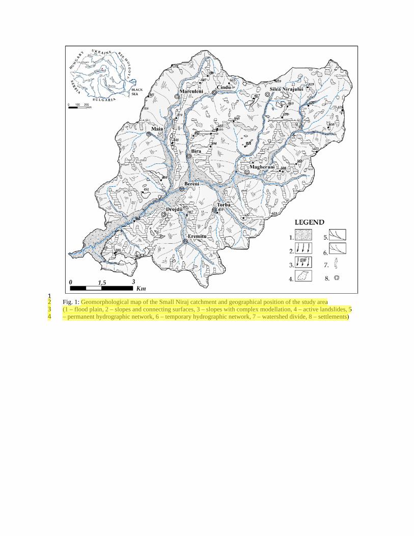
1 Fig. 1: Geomorphological map of the Small Niraj catchment and geographical position of the study area 2 (1 – flood plain, 2 – slopes and connecting surfaces, 3 – slopes with complex modellation, 4 – active landslides, 5 3 – permanent hydrographic network, 6 – temporary hydrographic network, 7 – watershed divide, 8 – settlements) 4 

1 Fig. 2: Applied methodological flow chart 2 

3 Fig. 3: Landslide susceptibility map generated using the logistic model 4 

1 Fig. 4: Area under the ROC curve for the training data (left) and the testing data (right) 2 

3 Fig. 5: Landslide susceptibility map generated using the BSA model 4 

5 

1 Fig. 6: Percentage distribution of active landslide on the probability classes and ROC curve value 2 

3  4 

Fig. 7: Regional differences of susceptibility classes obtained through BSA model or by applying logistic model 5 

6  7 Fig. 8: Comparative percentage distribution on susceptibility classes obtained by applying BSA model (8.A) and 8 logistic model (8.b) 9  10 

1