large scale evacuation transportation systems: robust ... · pdf filea new model for robust...
TRANSCRIPT

The Pennsylvania State University University of Maryland University of Virginia
Virginia Polytechnic Institute & State University West Virginia University
The Pennsylvania State University The Thomas D. Larson Pennsylvania Transportation Institute
Transportation Research Building University Park, PA 16802-4710 Phone: 814-865-1891 Fax: 814-863-3707
Large Scale Evacuation Transportation Systems:
Robust Models and Real Time Operations

Large Scale Evacuation Transportation Systems: Robust Models and Real Time Operations
FINAL REPORT
April 30, 2012
By Tao Yao
Technical Report Documentation Page1. Report No. PSU-2010-02
2. Government Accession No. 3. Recipient’s Catalog No.
4. Title and Subtitle
Large Scale Evacuation Transportation Systems: Robust Models and Real Time Operations
5. Report Date
August 2012
6. Performing Organization Code
MAUTC Project No. PSU2010-02 7. Author(s)
Tao Yao
8. Performing Organization Report LTI 2012-04
9. Performing Organization Name and Address
The Thomas D. Larson Pennsylvania Transportation Institute The Pennsylvania State University 201 Transportation Research Building University Park, PA, 16802-4710
10. Work Unit No. (TRAIS) 11. Contract or Grant No. DTRT07-G-0003
12. Sponsoring Agency Name and Address
US Department of Transportation Research and Innovative Technology Administration UTC Program, RDT-30 1200 New Jersey Ave., SE Washington, DC 20590
13. Type of Report and Period Covered
Final Report 4/1/2010-3/30/2012 14. Sponsoring Agency Code
15. Supplementary Notes 16. Abstract
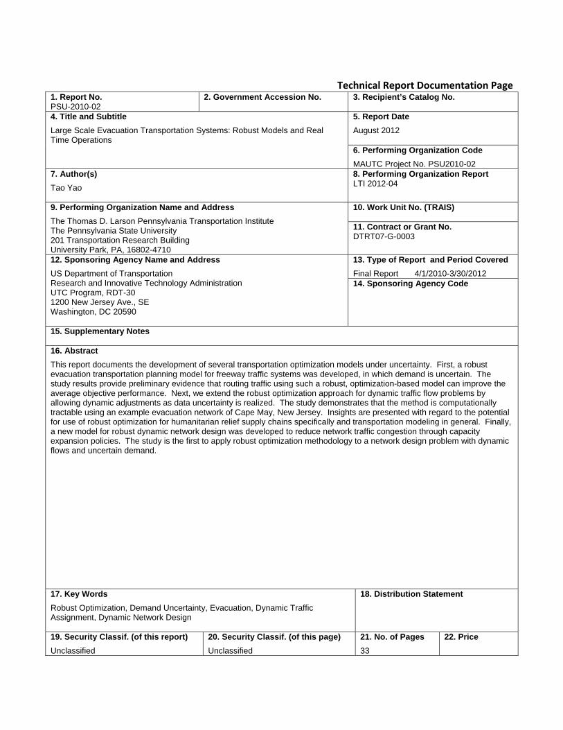
This report documents the development of several transportation optimization models under uncertainty. First, a robust evacuation transportation planning model for freeway traffic systems was developed, in which demand is uncertain. The study results provide preliminary evidence that routing traffic using such a robust, optimization-based model can improve the average objective performance. Next, we extend the robust optimization approach for dynamic traffic flow problems by allowing dynamic adjustments as data uncertainty is realized. The study demonstrates that the method is computationally tractable using an example evacuation network of Cape May, New Jersey. Insights are presented with regard to the potential for use of robust optimization for humanitarian relief supply chains specifically and transportation modeling in general. Finally, a new model for robust dynamic network design was developed to reduce network traffic congestion through capacity expansion policies. The study is the first to apply robust optimization methodology to a network design problem with dynamic flows and uncertain demand. 17. Key Words
Robust Optimization, Demand Uncertainty, Evacuation, Dynamic Traffic Assignment, Dynamic Network Design
18. Distribution Statement
19. Security Classif. (of this report)
Unclassified
20. Security Classif. (of this page)
Unclassified
21. No. of Pages
33
22. Price


TABLE OF CONTENTS
1 Introduction .......................................................................................................................... 1
2 Robust Optimization for Emergency Logistics Planning: Risk Mitigation in Humanitarian Relief Supply Chains ................................................................................. 1
2.1 Introduction ................................................................................................................ 1 2.2 Literature Review ....................................................................................................... 2 2.3 CTM for the DTA Problem ........................................................................................ 3 2.4 Robust Optimization Formulation of CTM ................................................................ 6 2.5 Emergency Logistics Management ............................................................................ 7
3 Robust Optimization Model for a Dynamic Network Design Problem Under Demand Uncertainty ........................................................................................................ 10
3.1 Introduction ................................................................................................................ 10 3.2 Literature Review ....................................................................................................... 11 3.3 Deterministic Model ................................................................................................... 12 3.4 Robust Formulation .................................................................................................... 14 3.5 Numerical Analysis .................................................................................................... 16
4 Conclusion ........................................................................................................................... 25
4.1 AARC Conclusions .................................................................................................... 25 4.2 RNDP Conclusions .................................................................................................... 26
References ................................................................................................................................ 27
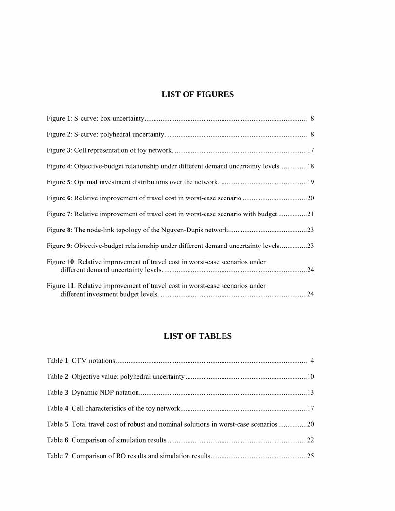
LIST OF FIGURES
Figure 1: S-curve: box uncertainty. .......................................................................................... 8
Figure 2: S-curve: polyhedral uncertainty. .............................................................................. 8
Figure 3: Cell representation of toy network. .......................................................................... 17
Figure 4: Objective-budget relationship under different demand uncertainty levels ............... 18
Figure 5: Optimal investment distributions over the network. ................................................ 19
Figure 6: Relative improvement of travel cost in worst-case scenario .................................... 20
Figure 7: Relative improvement of travel cost in worst-case scenario with budget ................ 21
Figure 8: The node-link topology of the Nguyen-Dupis network. ........................................... 23
Figure 9: Objective-budget relationship under different demand uncertainty levels. .............. 23
Figure 10: Relative improvement of travel cost in worst-case scenarios under different demand uncertainty levels. ................................................................................ 24
Figure 11: Relative improvement of travel cost in worst-case scenarios under different investment budget levels. .................................................................................. 24
LIST OF TABLES
Table 1: CTM notations. .......................................................................................................... 4
Table 2: Objective value: polyhedral uncertainty .................................................................... 10
Table 3: Dynamic NDP notation .............................................................................................. 13
Table 4: Cell characteristics of the toy network....................................................................... 17
Table 5: Total travel cost of robust and nominal solutions in worst-case scenarios ................ 20
Table 6: Comparison of simulation results .............................................................................. 22
Table 7: Comparison of RO results and simulation results ...................................................... 25


1. Introduction
This research focuses on the development of transportation optimization models under uncertainty. Yao et al. (2009) develop a robust evacuation transportation planning model for freeway traffic systems in which demand is uncertain. The study results provide preliminary evidence that routing traffic using such a robust, optimization-based model can improve the average objective performance. In Section 2 the authors describe the work of Ben-Tal et al. (2011), which extends the robust optimization approach for dynamic traffic flow problems by allowing dynamic adjustments as data uncertainty is realized. The study also demonstrates that the method is computationally tractable using an example evacuation network of Cape May, New Jersey. Insights are presented with regard to the potential for using robust optimization for humanitarian relief supply chains specifically and transportation modeling in general. Section 3 discusses the work of Chung et al. (2011), in which a new model for robust dynamic network design was developed to reduce network traffic congestion through capacity expansion policies. The study is the first to apply robust optimization methodology to a network design problem with dynamic flows and uncertain demand.
2. Robust Optimization for Emergency Logistics Planning: Risk Mitigation in Humanitarian Relief Supply Chains
2.1 Introduction
Over the past three decades, the number of reported disasters has risen threefold. Roughly 5 billion people have been affected by disasters with estimated damages of about $1.28 trillion (Guha-Sapir et al. 2004). Although most of these disasters could not have been avoided, significant improvements in death counts and reported property losses could have been made by efficient distribution of supplies. The supplies here could mean personnel, medicine, and food, which are critical in emergency situations. The supply chains involved in providing emergency services in the wake of a disaster are referred to as humanitarian relief supply chains. Humanitarian relief supply chains are formed within a short time period after a disaster, with the government and the NGOs being the major drivers of the supply chain. Clearly, emergency logistics is an important component of humanitarian relief supply chains.
Most literature in emergency logistics focuses on generating transportation plans for rapid dissemination of medical supplies inbound to the disaster-hit region (Sheu 2007, Ozdamar et al. 2004, Lodree Jr. and Taskin 2008). There is, however, another aspect of emergency logistics which is often ignored - outbound logistics. The outbound logistics considers a situation where people and emergency supplies (e.g., medical facilities and services for special need evacuees) need to be sent from a particular location affected by disaster within a given time horizon.
In the outbound emergency logistics, the demand of traffic flows is usually highly uncertain and depends on a number of factors, including the nature of the disaster (natural/man-made) and time of impact. This uncertainty in the demand causes disruptions in emergency logistics and hence disruptions in humanitarian relief supply chains, leading to severe sub-optimality or even infeasibility, which may ultimately lead to loss of life and property. In order to mitigate the risk of uncertain demand, we study the problem of generating evacuation transportation plans that are robust to uncertainty in outgoing demand. More specifically, we solve a dynamic (multi-period) emergency response and evacuation traffic assignment problem with uncertain demand at source nodes.
Researchers and practitioners in the field of transportation are concerned with multi-period management problems with an inherent time-dependent information uncertainty. Traditional dynamic optimization approaches for dealing with uncertainty (e.g., stochastic and dynamic programming) usually require the probability distribution for the underlying uncertain data to obtain expected objectives. However, in many cases, it may be very difficult to accurately identify the distribution required to solve a
2
problem. Especially, this is more likely true when one is considering an evacuation transportation problem due to the inherent complexity and uncertainty. In addition, the robust solution guaranteeing the feasible evacuation plan is important, since infeasible solutions may cause potential loss of life and property in extreme events.
The authors explore the potential of robust optimization (RO) as a general computational approach to managing uncertainty, feasibility, and tractability for complex transportation problems. The RO approach was originally developed to deal with static problems formulated as linear programming (LP) or conic-quadratic problems (CQP), using crude uncertainty with hard constraints. It means that uncertainty is assumed to reside in an appropriate set, and RO guarantees the feasibility of the solution within the prescribed uncertainty set by adopting a min-max approach. The RO technique has been successfully applied in some complex and large-scale engineering design and optimization problems, similar to robust control in control theory (Ben Tal and Nemirovski 1999, 2002).
The original RO approach considers static problems. The underlying assumption of RO is ``here and now'' decisions, and all decision variables need to be determined before any uncertain data are realized. This is not typical in many transportation management problems that have a multi-period nature. In multi-period transportation problems such as dynamic traffic assignment, “wait and see” decisions are made, which means some decision variables are “adjustable” and affected by part of the realized data. Recognizing the need to account for such dynamics, Ben Tal et al. (2004) extended the RO approach and developed an Affinely Adjustable Robust Counterpart (AARC) approach to consider “wait and see” decisions.
To demonstrate the use of AARC in emergency transportation management settings, in this research project we consider a system optimum dynamic traffic assignment (SO-DTA) problem. The main contributions are summarized as follows.
• We develop a robust optimization framework for system optimum dynamic traffic assignment problems. The framework incorporates a linear programming (LP) formulation based on the Cell Transmission Model (CTM) (Daganzo 1993, 1995, Ziliaskopoulos 2000) and the AARC approach by considering dynamical adjustments to realizations of uncertainty with appropriate uncertainty sets. The framework is converted to LP and hence is computationally tractable.
• This research applies the proposed robust optimization framework to an emergency response and logistics planning problem. Numerical examples are provided to illustrate the value of the robust optimization in the context of emergency logistics and demonstrate the computational viability of the developed framework. Simulation experiments show that the AARC solution provides excellent results when compared with the solutions of deterministic LP and Monte Carlo sampling-based stochastic programming.
• This research work obtains some general insights that may have wider applicability for transportation managers: (1) A robust solution may improve both feasibility and performance when infeasibility costs are significant. Intuitively, the usual nominal optimal solution may be not far from the robust solution, but the usual optimal solution can perform much worse in the worst case. (2) An integration of RO and transportation modeling will improve the generation, communication, and potential use of uncertainty data in logistics transportation management. The intuition for this insight is twofold. First, in many applications in transportation, the set-based uncertainty (used by RO) is the most appropriate notion of data uncertainty. Second, computational tractability (resulting from this set-based uncertainty and dynamic traffic flow modeling in LP formulations) leads to efficient solutions for logistics transportation management under uncertainty.
2.2 Literature Review
The DTA problem describes a traffic system with time-varying flow and has been studied substantially since the seminar work of Merchant and Nemhauser (1978a,b). The main research can be classified into four categories: mathematical programming, optimal control, variational inequality, and simulation-based approach (see Peeta and Ziliaskopoulos (2001), Friesz and Bernstein (2000) for a review).

3
Daganzo (1993, 1995) proposed the CTM model, consisting of a set of linear difference equations, to develop a theoretical framework to simulate network traffic. It was assumed that the best route from origin to destination is already known to the travellers. Ziliaskopoulos (2000) relaxed this assumption by formulating a single destination SO DTA problem as a linear program with the decision variables being the route choices. Recently, the deterministic CTM-based DTA model has been applied to evacuation management (e.g., Tuydes (2005), Chiu et al. (2007), Xie et al. (2010)). For example, Chiu et al. (2007) proposed a network transformation and demand modeling technique for solving an evacuation traffic assignment planning problem using the CTM-based single destination SO DTA model.
Recognizing that deterministic demand or network characteristics are unrealistic in some settings, another wave of research on DTA is the modeling of stochastic properties and the development of robust solutions. Waller et al. (2001) and Waller and Ziliaskopoulos (2006) addressed the impact of demand uncertainty and the importance of robust solution. Peeta and Zhou (1999) used Monte Carlo simulation to compute a robust initial solution for a real-time online traffic management system. Chance constraint programming for the SO DTA problem was analyzed by Waller and Ziliaskopoulos (2006). Yazici and Ozbay (2007) introduced probabilistic capacity constraint and solved the CTM-based SO DTA problem for a hurricane evacuation problem. Karoonsoontawong and Waller (2007) proposed a DTA-based network design problem formulated as a two-stage stochastic program and a scenario-based robust optimization (Mulvey et al. 1995). Ukkusuri and Waller (2008) proposed a two-stage stochastic program with recourse model to account for demand uncertainty.
Recently, robust optimization has witnessed a significant growth (Ben-Tal and Nemirovski 1998, 1999, 2000, El Ghaoui et al. 1997, 2003, Bertsimas and Sim 2003, 2004). For a summary of the state of art in RO, please refer to Ben-Tal et al. (2009), Bertsimas et al. (2011) and references therein. RO has been proposed for application in network and transportation systems (Bertsimas and Perakis (2005), Ordonez and Zhao (2007), Atamturk and Zhang (2007), Mudchanatongsuk et al. (2008), Erera et al. (2009), Yin et al. (2008, 2009) to name a few). Related to our work, Atamturk and Zhang (2007) proposed a robust optimization approach for two-stage network flow and design. Erera et al. (2009) developed a two-stage robust optimization approach for repositioning empty transportation resources. Both of the studies are in the spirit of Ben-Tal et al. (2004), where the second-stage variables are determined as recourse or recovery actions while maintaining feasibility after the uncertain data are realized.
2.3 CTM for the DTA Problem
In this section, we summarize and reformulate the prior work on the deterministic linear program (DLP) based on the traditional CTM model (Ziliaskopoulos 2000). The CTM, named by Daganzo (1993, 1995), models freeway traffic flow using simple difference equations. It approximates the kinematic wave model under the assumption of a piecewise linear relationship between flow and density on the link. More formally, the following equation shows the relationship between traffic flow, q, and density on a link, k, in a traffic network.
( )( ),,,min= maxmax kkwqvkq −
where v is free flow velocity, maxk is maximum possible density, w is backward wave speed and
maxq is maximum allowable flow on the link. The LP-based CTM model of Ziliaskopoulos (2000) is a simplification of the original CTM model. In
the CTM model, a segment of a freeway is decomposed into cells based on the free flow velocity and length of discrete time step. By this division, vehicles can move only to adjacent cells in unit time. The connectors between cells are dummy arcs indicating the direction of flow between cells. The demand of the CTM model represents the vehicular trips for each OD pair. In other words, each demand has its own origin and destination node in the network. The demand for each OD pair is assumed to be known at the beginning and used as input data of the CTM model. However, in our model, demand at the source node is uncertain. We provide the reformulation of the deterministic LP-based CTM model. The model

4
includes the characteristics of time-space dependent cost and an adjacent matrix. In the traditional CTM research, it is assumed that the coefficient of cost is a constant value within the time-space network. However, in this report, the coefficient is assumed to be dependent on time horizon and demand nodes. It is a more common situation and is necessary to study emergency logistics management. An adjacency matrix A = [ ija ] is defined for representing the connectivity of the cells. The value of ija is equal to 1 if cell i is connected to cell j, otherwise ija =0.
Table 1: CTM notations
Symbol Description
ℑ : set of time intervals, { }T1,.., C : set of cells, { }I1,..,
SC : set of sink cells
RC : set of source cells
A : adjacency matrix representing transportation network connectivity. tic :
time-space dependent cost in cell i at time t
tix :
number of vehicle contained in cell i at time t
tijy :
number of vehicle flowing from cell i to cell j at time t
tid :
demand generated in cell i at time t
tiN :
capacity of cell i at time t
tiQ :
inflow/outflow capacity of cell i at time t
tiδ :
traffic flow parameter for cell i at time t
ix̂ : initial occupancy of cell i
Based on the notations in Table 1, we present the deterministic linear programming (DLP) model:
)(min\,
DLPMxc ti
ti
sCCityx−∑∑
∈ℑ∈
(1)
tosubject
ℑ∈∈∀≥+−− −−
∈
−
∈
− ∑∑ tCidyayaxx ti
tijij
Cj
tkiki
Ck
ti
ti ,,1111 (2)
ℑ∈∈∀≤∑∈
tCiQya ti
tkiki
Ck,, (3)
ℑ∈∈∀≤+∑∈
tCiNxya ti
ti
ti
ti
tkiki
Ck,,δδ (4)

5
ℑ∈∈∀≤∑∈
tCiQya ti
tijij
Cj,, (5)
ℑ∈∈∀≤−∑∈
tCixya ti
tijij
Cj,0, (6)
Cixx ii ∈∀,ˆ=0 (7)
CCjiyij ×∈∀ ),(0,=0 (8)
ℑ∈∀∈∀≥ tCixti ,0, (9)
ℑ∈∀×∈∀≥ tCCjiytij ,),(0, (10)
The cost parameter tic depends on time in order to give a penalty when any people cannot arrive at the
destination at the end of time horizon T. i.e.
⎩⎨⎧
∈≠∈
,=,\,\1
=TtCCiMTtCCi
cs
sti
where M is assumed to be a positive large number to represent the unsatisfied demand cost. By using the time-dependent cost parameter, the objective function measures the total cost incurred, which consists of travel cost and penalty cost. The objective function of the LP-based CTM model (M-DLP) provides an optimistic estimate or lower bound of total cost as it simplifies the original CTM model by Daganzo (1993, 1995) and allows vehicle holding.
The dynamics of the system are that the change of traffic level is determined by traffic flow and demand at each node and in each time period. By letting demand be 0 everywhere except source cells, the formulation can be generalized by Equation 2. The total inflow into a cell is bounded by not only the inflow capacity (Equation 3) but also by the remaining capacity of the cell (Equation 4). Similarly, total output flow from a cell is limited by the outflow capacity (Equation 5) and the current occupancy of the cell (Equation 6). It is assumed that the capacities of source and sink cells are infinite. The initial conditions and non-negativity conditions are considered as the remaining constraints. Note that Equation 9 is a redundant constraint, since 0≤−∑ ∈
ti
tijijCj
xya , 0≥tijy and 0≥ija . It is evident that
ti
tijijCj
xya ≤≤∑ ∈0 and Equation 9 can be eliminated.

6
2.4 Robust Optimization Formulation of CTM
The CTM-based SO DTA problem is a generic multi-period linear programming problem. In this section, we apply AARC methodology to deal with the uncertainty in demand and find a robust solution for the multi-period emergency logistics problem.
In RO approach, it is assumed that demand tid is unknown and it belongs to a prescribed uncertainty
set. In particular, a box uncertainty set is generally used. )],(1~),(1~[=],[ θθ +−≡∈ t
it
it
iti
bd
ti ddddUd
where θ is uncertainty level and tid~ is nominal demand in cell i during time interval t.
In order to find a less conservative solution, we consider a joint constraint where the demands are upper bounded. Let's consider Ri
tiTt
CiDd ∈∀≤∑ ∈, , which refers to a joint budget for demand
uncertainty. This represents the situation that the total demand ( tiTt
d∑∈) from a source node is limited by
an upper bound ( iD ). The box uncertainty set in conjunction with the budget uncertainty set becomes a polyhedral uncertainty set, which can be a more realistic assumption in emergency logistics management. Now we have the following uncertain data set.
⎭⎬⎫
⎩⎨⎧
≤≤≤≡∈ ∑∈
iti
Tt
ti
ti
ti
ti
pd
ti DdddddUd ,:
Next, a specific form of linear decision rules is assumed to convert M-DLP to AARC formulation. The linear rules are used to derive a computationally tractable problem by approximating the robust solution. We note that the solution from AARC is optimal in worst case from the predetermined uncertainty set. However, there is no guarantee that the robust solution is close to optimal in the other cases, since the relationship between uncertain parameters and decision variables may not be linear. Specifically, the adjustable control variables, t
ijy , can be represented as an affine function of previously observed demand
values, i.e., τττππ s
sijt
tIRCsijttij dy ∑∑ ∈∈
− +1= , where 1−ijtπ and τπ s
ijt are non-adjustable variables and
{ }10,..,= −tIt . Along with the affine rule of control variables, the state variables also become an affine function of the
previously realized data, ,= 1 τττηη s
sit
tIRCsitti dx ∑∑ ∈∈
− + by the linear structure of the CTM model.
By substituting the state and control variables, we have the following AARC formulation.
)(,1,,1,
AARCMzmin −−− ηηππσ
(11)
..ts
dtis
sit
tIRCsit
ti
Cit
Udzdc ∈∀≤+ ∑∑∑∑∈∈
−
∈ℑ∈
,)( 1 ττ
τ
ηη
)()()( 1
1
111
1
11
1 ττ
τ
ττ
τ
ττ
τ
ππηηηη sskit
tIRCskitki
Cks
sit
tIRCsits
sit
tIRCsit dadd −
−∈∈
−−
∈−
−∈∈
−−
∈∈
− ∑∑∑∑∑∑∑ +−+−+
ℑ∈∈∀≥++ −−
−∈∈
−−
∈∑∑∑ tCidda t
issijt
tIRCsijtij
Cj
,,)( 11
1
11
ττ
τ
ππ

7
ℑ∈∈∈∀≤+ ∑∑∑∈∈
−
∈
tCiUdQda dti
tis
skit
tIRCskitki
Ck
,,,)( 1 ττ
τ
ππ
ℑ∈∈∈∀≤+++ ∑∑∑∑∑∈∈
−
∈∈
−
∈
tCiUdNdda dti
ti
tis
sit
tIRCsit
tis
skit
tIRCskitki
Ck,,,)()( 11 δηηδππ ττ
τ
ττ
τ
ℑ∈∈∈∀≤+ ∑∑∑∈∈
−
∈
tCiUdQda dti
tis
sijt
tIRCsijtij
Cj
,,,)( 1 ττ
τ
ππ
ℑ∈∈∈∀≤+−+ ∑∑∑∑∑∈∈
−
∈∈
−
∈
tCiUddda dtis
sit
tIRCsits
sijt
tIRCsijtij
Cj
,,0,)()( 11 ττ
τ
ττ
τ
ηηππ
Cixii ∈∀− ,ˆ=10η
( ) CCjiij ×∈∀− ,0,=10π
dtis
sijt
tIRCsijt UdtCCjid ∈ℑ∈×∈∀≥+ ∑∑
∈∈
− ,,),(0,1 ττ
τ
ππ
The formulation (M-AARC) is intractable since it is a semi-infinite program, and it can be reformulated as a tractable optimization problem as shown in the Theorem 1 (See Ben-Tal et al. 2011 for extensive results). The minimum objective value z, denoted as *
AARCz , is a guaranteed upper bound value for all realization of uncertain data under the assumption of linear dependency. The objective value,
*AARCz , also can be interpreted as the optimistic estimate of total travel cost in the worst case, which can
be lower than the optimistic estimate from robust counterpart(RC), *RCz as AARC has a larger robust
feasible region (Ben-Tal et al. 2004). The decision variables of AARC are not adjustable control and state variables, but a set of coefficient of affine functions of the control variables. This means that the solution of AARC is the linear decision rule.
2.5 Emergency Logistics Management
Emergency management is one of the best application areas for applying robust optimization due to the uncertainty of human beings and disaster. Robust solution, especially the AARC solution, can play an important role for emergency logistics planning for several reasons. First of all, the role of hard constraint is emphasized since the penalty cost for an infeasible solution is loss of life or property. Next, it is very difficult to estimate or forecast the demand model in the to-be-affected areas due to unexpected human behavior and the nature of disaster. Finally, we can take advantage of updated or realized data on demand by employing the AARC solution. When we solve M-AARC1, the optimal coefficients of the Linear Decision Rule (LDR) are computed offline. Going online, the actual decision variables (flows) are determined for period t by inserting the revealed uncertainties from previous periods in the LDR. A fully online version of the method can be also implemented. In such a version, at period t only the t-period design variables are activated. The horizon is then rolled forward and the problem is resolved after adjusting the stated variables revealed in previous periods.
In this section, an emergency logistics planning problem is considered and the meaning of demand uncertainty sets is explained. Then, we present a summary of experiments to test the performance of the

8
AARC approach. The AARC solution is benchmarked against an ideal solution with complete future information, deterministic LP, and sampling-based stochastic programming. Two test networks were chosen from Chiu et al. (2007) and Yazici and Ozbay (2007) for the numerical analysis.

9
2.5.1 Demand Modeling In an emergency logistics
problem, a general approach to model time-varying evacuee demand is captured by the following steps: The first step of demand modeling is calculation of total demand. Next, demand arrival or vehicle departure rate is determined for describing a dynamic environment. For example, an S-shape curve can be used to represent the cumulative percentage of demand arrival. In most studies, it is assumed that the parameters (e.g., slope) of S-curve are unknown but a deterministic value. Since the parameters can be estimated with empirical data or simulation results, different research has shown different values (Radwan et al. 1985, Lindell 2008). However, in the real world, both the total number of demand and the departure rate are uncertain. By considering a box uncertainty or polyhedral uncertainty set, we can overcome the limitation of the deterministic S-curve and cover an infinite number of S-curves, including fast, medium, and slow response. Figure 1 shows the S-curve with upper and lower bound defined by box uncertainty. In Figure 2, polyhedral uncertainty set (box uncertainty and budget uncertainty) is shown and the upper bound of S-curve is limited by total demand.

10
2.5.2 Small Network Example In the first numerical experiment, a small network configuration is used to verify the performance of
AARC from the illustrative example of Chiu et al. (2007). The network consists of 14 nodes, including 3 source nodes and 1 super sink cell. The data of the transportation network is adopted from Chiu et al. (2007) except demand data, since deterministic demand was used in the original model. Also, we assume that the penalty cost (M) for unmet demand is 100.
As mentioned before, we consider uncertain multi-period demand. In particular, the following mathematical formulation of the S-curve (Radwan et al. 1985) is adopted for demand loading.
))),((exp1/(1=)( βα −−+ ttP
where P(t) is the cumulative distribution with α = 1, the slope of curve, and β = 3, the median departure time. In both box and polyhedral uncertainty set, nominal demand at time t is calculated by multiplying (P(t) − P(t − 1)) with expected total demand. Also, the joint budget of demand uncertainty is assumed to be one and one-half times the sum of expected total demand. 2.5.3 AARC vs. DLP
Based on the nominal data, uncertain demand in a polyhedral set is generated and tested. The uncertainty level θ is increased from 2.5% to 30%. First, objective values are calculated and emergency logistics plans are generated using M-DLP and M-AARC. Next, given the uncertainty level and evacuation plan, a simulated (or realized) objective value from Equation 1 is computed by generating random demand in the specified uncertainty set. Average values, standard deviation, and the worst-case solution of 1,000 simulated objective values are used to compare the traffic assignment solutions.
The first objective of our experiments is a comparison of AARC and DLP under a polyhedral uncertainty set. Objective values of robust optimization approaches, which measure the worst case solution of the vehicle control plan, are computed and compared in Table 2 by changing the uncertainty level. DLP solution shows the cost when only deterministic nominal demand is dealt with. It is natural that the objective value of AARC with larger uncertainty level is bigger. Also, the objective value of DLP is smaller, since it is equivalent to AARC with zero uncertainty level.
In simulation, the emergency logistics plan from inequality flow constraints has to be adjusted in some way, since we relaxed the constraint in Equation 2. We assumed that if there are fewer vehicles in a node than the vehicle flow plan, proportionate flow is allocated to each path. Also, any vehicles exceeding the plan will remain at the node and pay a penalty for not planning them. Table 2 shows the simulated objective value of ideal DLP, DLP, and AARC. Ideal DLP is the case where perfect future demand information is known at the beginning of the planning horizon. It is the lower bound of the simulated objective value. The average improvement of AARC over DLP is significant at a higher uncertainty level.
The AARC problem with 14 nodes and 15 planning horizon has 36,600 constraints and 190,428 variables. It is solved in about 44 seconds on a PC with Intel processor 1.87 GHz and 2 GB of memory.

11
Table 2: Objective value: polyhedral uncertainty
obj avg sd worst
θ DLP AARC Ideal DLP AARC Ideal DLP AARC Ideal DLP AARC
0.025 350.10 358.18 354.35 417.13 355.34 1.08 15.14 0.91 356.54 452.33 357.17
0.05 350.10 366.27 358.59 484.25 359.70 2.16 30.19 1.76 362.97 554.56 363.27
0.075 350.10 375.24 362.85 551.49 364.88 3.26 45.10 2.97 369.83 656.80 370.73
0.1 350.10 384.35 367.33 618.81 370.72 4.57 59.95 3.78 377.14 759.03 378.44
0.15 350.10 402.57 376.78 753.49 381.79 7.20 89.63 5.35 391.76 963.49 393.29
0.2 350.10 420.80 386.35 888.23 397.50 9.70 119.29
6.14 406.38 1167.95 410.64
0.25 350.10 439.03 395.95 1023.00 410.17 12.17 148.94
7.90 421.00 1372.42 427.02
0.3 350.10 457.25 405.55 1157.77 420.57 14.63 178.59
10.12 435.61 1576.88 441.57
3. Robust Optimization Model for a Dynamic Network Design Problem Under Demand Uncertainty
3.1 Introduction
Network design consists of a broad spectrum of problems, each corresponding to different sets of objectives, decision variables and resource constraints, implying different behavioral and system assumptions, and possessing varying data requirements and capabilities in terms of representing network supplies and demands. Network design models have been extensively used as various types of strategic, tactical and operational decision-making tools and spanned over a variety of applications in, for example, transportation, production, distribution, and communication fields. In a transportation network, traffic congestion has long been a major concern of the network operator, occuring when traffic volumes exceed the road capacity. Network design problems (NDP) for transportation networks in general aim at minimizing network traffic congestion (or minimizing some general network-wide traveler costs) through implementing an optimal capacity expansion policy in the network.
An optimal capacity expansion policy, however, may not be reached without properly considering the behavioral nature of travel demands, which are inherently time-variant and uncertain. Travel demands are an aggregate result of individual travel activities, which are determined by various observed and unobserved socioeconomic factors and subject to geographical, technological, and temporal constraints. The vast body of the literature has focused on static deterministic NDPs (see, for example, Magnanti and Wong 1984; Minoux 1989; Yang and Bell 1998). A major limitation of static network design models is the inability to capture traffic dynamics, such as traffic shockwave propagation and the buildup and avoidance of queues. Dynamic models, on the other hand, allow us to model the time-dependent

12
variation of traffic flows and travel behaviors and hence better describe traffic evolution and interaction phenomena over the network (Peeta and Ziliaskopoulos 2001). Travel demand uncertainty is not only the underlying characteristic of travel activities but also a likely result of our inaccurate or inconsistent travel demand estimation procedures. Without explicit and rigorous recognition of uncertainty in travel demands, any transportation network development plans and policies may take on unnecessary risk and even result in misleading outcomes (Zhao and Kockelman 2002).
The focus of this research is on a robust optimization (RO) based dynamic NDP under demand uncertainty, or more succinctly, a robust dynamic NDP (RDNDP). The research community has observed a number of recent network design studies that explicitly incorporate demand uncertainty into NDPs with time-varying flows (see Waller and Ziliaskopoulos 2001; Karoonsoontawong and Waller 2007; Ukkusuri and Waller 2008). The common feature of these problems is that time-varying flows are described by the cell transmission model (CTM) (Daganzo 1994, 1995) and the network flow pattern is then characterized by CTM-based dynamic traffic assignment (DTA) methods, under either the system-optimal (Ziliaskopoulos 2000) or user-optimal assignment mechanism (Ukkusuri and Waller 2008). The demand uncertainty of these problems is accommodated by a chance constraint setting, a two-stage recourse model, or a scenario-based simulation method. These techniques, however, suffer from deficiencies related to lack of data availability and problem tractability, which limit their applicability to a broad range of applications. Resulting models from these stochastic modeling methods are often computationally intractable and require known probability distributions.
We follow a similar fashion to form our RDNDP using the CTM-based system-optimal DTA model, but employ the RO approach to account for demand uncertainty. Given the fact that the CTM-based DTA model has a linear programming (LP) formulation, we use the set-based RO method (Ben-Tal and Nemirovski 1998, 1999, 2000, 2002) to form a tractable LP model for the RDNDP, which overcomes the limitations of previous stochastic optimization methods. Specifically, in our RDNDP, no probability distribution is presumed; instead, we only need to simply specify an uncertain set, which is readily available in most applications. The solution feasibility is guaranteed by the RO method through the use of the prescribed uncertainty set and can be readily made computationally tractable through an appropriate reformulation.
The main contributions of this work can be summarized as follows: • The authors developed an RO framework for the RDNDP. For simplicity, we present our RO
model only for single-destination, system-optimal networks. However, the basic RO counterpart formulation method can be readily transferred to the user-optimal and multi-destination problem cases. This work adds to the body of knowledge in dynamic network design by presenting an emerging method related to the solution robustness.
• An appealing feature of our robust counterpart problem is that it still has an LP formulation, so it is in general computationally tractable and can be solved in polynomial time by a few well-known solution algorithms.
• Our numerical experiments demonstrate the value of RO in the context of dynamic traffic assignment and network design problems. The computational viability is illustrated for the proposed modeling framework. The numerical analysis for the impact of a bounded investment budget and demand uncertainty level on network design solutions justifies the solution robustness.
3.2 Literature Review
Numerous NDPs for transportation applications have been presented in the past three decades (see Magnanti and Wong 1984; Minoux 1989; Yang and Bell 1998). These NDPs are distinguished by a variety of problem settings and supply and demand assumptions. The literature review presented in this section by no means provides a comprehensive survey of general network design problems or of network design applications in the transportation field; instead, our discussion is focused on those network design

13
models and solution methods with data uncertainty, particularly network design problems with time-varying flows.
A great amount of attention has been paid to NDPs with data uncertainty in past years, and various modeling techniques have been used for dealing with uncertain input data and parameters. The main approaches can be classified into two groups: stochastic programming (SP) and robust optimization (RO). The SP approach requires known probability distributions of the uncertain data and includes techniques such as the Monte Carlo sampling approach and chance-constrained programming. For example, Waller and Ziliaskopoulos (2001) solved an NDP under uncertain demands where the probability distributions of demand rates are known a priori. They used a CTM-based, system-optimal NDP formulation with chance constraints. Ukkusuri and Waller (2008) extended the CTM to model both the system-optimal and user-optimal NDPs and presented the formulations of a chance-constrained NDP model and a two-stage resource NDP model to account for demand uncertainty.
Mulvey et al. (1995) proposed a scenario-based RO approach for general LP problems. Karoonsoontawong and Waller (2007) applied this approach to a CTM-based dynamic NDP with stochastic demands under both the system-optimal and user-optimal conditions. A similar RO model formulation approach was employed by Ukkusuri et al. (2007), in which a scenario-based robust NDP with discrete decision variables was tackled by a genetic algorithm. The limitations of a scenario-based RO approach are similar to stochastic programming in that we must know the probability of each scenario in advance, and it is computationally expensive when there are a large number of scenarios.
Recently, a variety of papers have used the set-based RO technique to characterize optimization models with data uncertainty. Interested readers are referred to Ben-Tal and Nemirovski (2002) and Bertsimas et al. (2011) for reviews of the set-based RO methods. For NDPs with stochastic demands, Ordonez and Zhao (2007) formulated and solved a static multicommodity NDP with demand and travel time uncertainties bounded by polyhedral sets. Mudchanatongsuk et al. (2008) extended the work by Ordonez and Zhao by considering some generalized assumptions on demand uncertainty, in which they discussed a path-constrained NDP and introduced a column generation method to solve the robust NDP with polyhedral uncertainty sets. Atamturk and Zhang (2007) formulated and solved a NDP by using the two-stage RO method and taking advantage of the network structure for its solutions. To characterize their uncertainty sets they used a budget of uncertainty, which limits the number of observed demand values that can differ from nominal values. They also discussed the numerical results for a simple location-transportation problem and compared the two-stage robust approach with the single-stage robust approach as well as two-stage, scenario-based stochastic programming.
There have also been approaches where the set-based RO approach is used to construct discrete network design models. For example, Lou et al. (2009) described a discrete NDP with user-equilibrium flows based on the concept of uncertainty budget and proposed a cutting-plane method for problem solutions; Lu (2007) addressed a discrete user-equilibrium NDP with polyhedral uncertainty sets using the RO approach and used an iterative solution algorithm to solve the problem.
To the best of our knowledge, no work has been done in applying the set-based RO technique to investigate a NDP with dynamic flows and uncertain demands. In this work, our effort is given to analytically developing and numerically analyzing the robust counterpart model of such an NDP in the context of transportation network design.
3.3 Deterministic Model
This section presents the deterministic version of the dynamic NDP model we have discussed, or the DDNDP model in abbreviation, which provides the basic modeling platform and functional form for the RDNDP model we will introduce in the next section. For discussion convenience, let us first present the notation used throughout these models (see Table 3).

14
Table 3: Dynamic NDP notation Sets Description τ Set of discrete time intervals, },...,1{ T
C Set of cells, },...,1{ I , including the set of sink cells ( SC ) and the set of source cells
( RC )
A Adjacency matrix, }{ ijaA= , where each ),( ji component, ija , equals 1 if cell i is
connected to cell j , and equals 0 otherwise Parameters Description
tid Demand generated in cell i at time t tic Travel cost in cell i at time t
tiN Capacity in cell i at time t
tiQ Inflow/outflow capacity of cell i at time t tiδ Ratio of the free-flow speed over the backward propagation speed of cell i at time t ix̂ Initial number of vehicles of cell i
B Total investment budget available for capacity expansion if Conversion coefficient of investment cost of cell i for a unit increase of ib
iχ Increase in capacity of cell i for a unit increase of ib
iϕ Increase in inflow/outflow capacity of cell i for a unit increase of ib Variables Description
ib Investment cost spent on cell i tix Number of vehicles staying in cell i at time t tiy Number of vehicles moving from cell i to cell j at time t
The network design problem aims at minimizing the sum of the total system travel cost and the
capacity expansion cost. To avoid the permanent traffic holding phenomenon, the travel cost in cell i at time t , t
ic , is set as follows:
⎩⎨⎧
=∈≠∈
=TtCCiMTtCCi
cS
Sti ,\
,\ 1
where M is a sufficiently large, positive number. The big- M value can also simply serve as a penalty cost, for example, in emergency evacuation networks, representing the potential loss of life and property caused by vehicles that do not arrive at the destination by the end of the time horizon. Use of the penalty cost has the effect of minimizing the number of vehicles staying in an evacuation network.
Now the DDNDP model can be written, using the notation listed in Table 1:
∑∑ ∑∈∈ ∈
+SS CCi
iit CCi
ti
tibyx
bfxc\\,,
minτ
subject to

15
τ∈∀∈∀=+−− −
∈
−
∈
−− ∑∑ tCidyayaxx ti
Cj
tijij
Ck
tkiki
ti
ti , 1111 (1)
τϕ ∈∀∈∀+≤∑∈
tCibQya iiti
Ck
tkiki , (2)
τχδδ ∈∀∈∀+≤+∑∈
tCibNxya iiti
ti
ti
ti
Ck
tkiki , )( (3)
τϕ ∈∀∈∀+≤∑∈
tCibQya iiti
Cj
tijij , (4)
τ∈∀∈∀≤−∑∈
tCixya ti
Cj
tijij , 0 (5)
BbCi
i ≤∑∈
(6)
Cixx ii ∈∀= ˆ0 (7)
CCjiyij ×∈∀= ),( 00 (8)
τ∈∀∈∀≥ tCix ti , 0 (9)
τ∈∀×∈∀≥ tCCjiy tij ,),( 0 (10)
Cibi ∈∀≥ 0 (11)
The objective function includes both the travel cost and expansion cost. Note here that the expansion
cost appears in the objective function and is subject to the investment budget constraint, which makes this formulation different from the traditional charge design problem (where the expansion cost term is only included in the objective function) and budget design problem (where the expansion cost term only appears in the investment budget constraint).
The constraint set of the DDNDP model specifies the capacity expansion limit, flow conservation and propagation relationships, initial network conditions and flow non-negativity conditions. The flow conservation constraint (i.e., Equation 1) for cell i at time t can be generalized by setting t
id to be zero in ordinary and sink cells. Constraints 2 and 4 are the bounds for the total inflow rate and total outflow rate of cell i at time t . Equation 3 bounds the total inflow rate into a cell by its remaining space, and Equation 5 bounds the total outflow rate of a cell by its current occupancy. Equation 6 sets the upper bound on the sum of capacity investments over all cells. The remaining constraints from Equation 7 through Equation 11 set initial network conditions and flow non-negativity conditions.
3.4 Robust Formulation
Now we develop the robust counterpart of the DDNDP model, which incorporates the demand uncertainty into an LP program via the RO approach. In the deterministic version, Equation 1 is the only set of constraints related to the demand generation. This equality constraint can be rewritten as an inequality constraint (Waller and Ziliaskopoulos 2006),
1111 −
∈
−
∈
−− ≥+−− ∑∑ ti
Cj
tijij
Ck
tkiki
ti
ti dyayaxx . (12)

16
It is assumed that all possible demand instances of tid belong to a box uncertainty set,
)],1(),1([ ti
ti
ti
tid
ddU ti
θθ +−= (13)
where tid is the nominal demand level and t
iθ is the demand uncertainty level. Then, the robust counterpart of Equation 12 with demand uncertainty becomes
111111 , −∈≥+−− −−
∈
−
∈
−− ∑∑ tid
ti
ti
Cj
tijij
Ck
tkiki
ti
ti Uddyayaxx . (14)
This is equivalent to the following inequality, 1
111
11
max −
∈∈
−
∈
−−
−−
≥+−− ∑∑ ti
UdCj
tijij
Ck
tkiki
ti
ti dyayaxx
tid
ti
, (15)
which becomes the flow conservation constraint for the RDNDP model. The above conversion of the flow conservation constraint leads the RDNDP to be in a deterministic functional form with the maximum possible demand in the box uncertainty set. Given that other constraints can be directly transferred from the DDNDP model to the RDNDP model, the RDNDP formulation can be written into the following LP form:
∑∑ ∑∈∈ ∈
+SS CCi
iit CCi
ti
tibyx
bfxc\\,,
minτ
subject to
τθ ∈∀∈∀+=+−− −−
∈
−
∈
−− ∑∑ tCidyayaxx ti
ti
Cj
tijij
Ck
tkiki
ti
ti , )1( 11111
(16)
τϕ ∈∀∈∀+≤∑∈
tCibQya iiti
Ck
tkiki ,
τχδδ ∈∀∈∀+≤+∑∈
tCibNxya iiti
ti
ti
ti
Ck
tkiki , )(
τϕ ∈∀∈∀+≤∑∈
tCibQya iiti
Cj
tijij ,
τ∈∀∈∀≤−∑∈
tCixya ti
Cj
tijij , 0
BbCi
i ≤∑∈
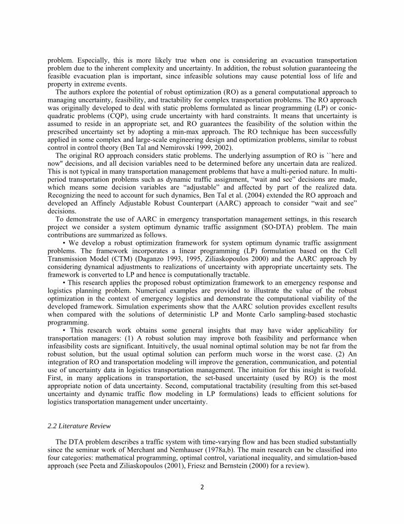
17
Cixx ii ∈∀= ˆ0
CCjiyij ×∈∀= ),( 00
τ∈∀∈∀≥ tCix ti , 0
τ∈∀×∈∀≥ tCCjiy tij ,),( 0
Cibi ∈∀≥ 0
18
In Equation 16, the value of )1( 11 −− + ti
tid θ is the maximum possible demand in cell i at time 1−t ,
according to the uncertainty set 1−tid
U , which represents the worst-case scenario. Therefore, the optimal
solution will remain feasible for all instances of demand. In other words, we will obtain an optimal solution with the cell capacity values that are adequate for any realized demand scenarios within the uncertainty set 1−t
idU .
When other types of uncertainty sets such as an ellipsoidal uncertainty set or a polyhedral uncertainty set are assumed, different deterministic formulations are derived. For example, the equivalent tractable robust counterpart with an ellipsoidal uncertainty set is a conic quadratic problem; if a polyhedral uncertainty set is assumed, it becomes a linear problem (see Yao et al. 2009 for details).
Property 1. The optimal objective function value of the RDNDP monotonically decreases with respect
to the investment budget level. Proof. Let the objective function of RDNDP be )(* Bzr , given the total budget level B Without loss
of generality, we assume that two budget levels 1B and 2B are given as 21 BB < . Since the RDNDP
with 2B has a larger feasible region than the RDNDP with 1B , )( 1* Bzr is smaller than or equal to
)( 2* Bzr , i.e. )()( 2
*1
* BzBz rr ≤ . ■
3.5 Numerical Analysis
The purpose of presenting computational experiments in this section is twofold: (1) to demonstrate the difference between robust network design solutions and corresponding nominal solutions from DDNPP; and (2) to illustrate the advantage of the RO approach for network design under demand uncertainty. Two numerical examples are selected from the literature for the experiments: (1) a smaller network with 16 cells and 15 time intervals; and (2) a larger network with 167 cells and 300 time intervals. For each example, the authors derived the optimal capacity investment solutions and the objective function values from the DDNPP and RDNDP models with various demand uncertainty levels. To evaluate the solution robustness, we also conducted a parallel simulation experiment to randomly generate 100 demand instances within the given box uncertainty set. The objective function values from the simulation experiment are also evaluated by solving the embedded DTA problem based on the same capacity expansion scheme as the one derived by the RDNDP model.
3.5.1 A Toy Network The first experiment uses the test network shown in Figure 3 and the data set in Table 4, which are
from Ukkusuri and Waller (2008). Since they considered a set of deterministic demands, it was assumed that the demand data in their paper are nominal values of the network design problem under uncertainty. Let us assume that uncertain demands from source cell 1 and 14 are [2(1- θ ), 2(1+ θ )] at time 0 and 1, and [1(1- θ ), 1(1+ θ )] at time 3. Note that when θ is equal to 0, the uncertainty sets become the nominal values. The investment cost coefficient ( if ) and penalty cost ( M ) for this example are set to 0.1 and 10, respectively.

19
Figure 3: Cell representation of the toy network (Ukkusuri and Waller 2008)
Table 4: Cell characteristics of the toy network (Ukkusuri and Waller 2008) Cell 2 3 4 5 6 7 8 9 10 11 12 15 16
tiN
4 4 4 4 4 2 4 4 4 4 4 4 4
tiQ
1 2 2 2 1 2 1 2 1 2 1 1 1
ix̂
0 0 0 0 0 0 0 0 0 0 0 0 0
3.5.1.1 Optimal Solutions under Different Uncertain Levels
The objective function value is calculated and plotted as the total budget level is varied from 0 to 80 in
the interval of 1 unit. Figure 4 shows the change of the objective function values of the DDNDP and RDNDP models with three different uncertainty levels (including, θ = 0.1, 0.2 and 0.3). As the budget level increases, the objective function value of the RDNDP model decreases and it converges to a certain value. Robust solutions are the best worst-case solutions and thus their objective function values are greater than those of the corresponding deterministic cases. Note that any nominal solution is equivalent to its robust solution with the zero uncertainty level (θ = 0).

20
Figure 4: The objective-budget relationship under different demand uncertainty levels
In all the above cases, the same cells (including cells 7, 9, 11, 15 and 16) are chosen for capacity
expansion, which indicates that they are bottleneck cells in the network. However, the proportions of the investment on the cells are dependent on the investment budget level and the demand uncertainty level. Figure 5 shows the investment distribution over the cells. The implication behind these distribution curves is that the investment strategy should be changed depending on the budget bound we set and the demand uncertainty degree we expect to face.
It is readily observed that there is a critical/maximum investment point associated with the investment budget level, beyond which a higher investment does not reduce the travel cost, or a higher investment even increases the objective function value if it is used for capacity expansion in the network. For example, this maximum investment point is between 30 and 40 monetary units in the DDNDP case, and the point is about 70 monetary units in the RDNDP case with θ = 0.3. The critical investment point can be interpreted as the threshold for investment: when the budget is less than this threshold, the marginal travel cost (reduction) is greater than the marginal construction cost (increase); when the budget is greater than the threshold, the marginal travel cost (reduction) is less than the marginal construction cost (increase).

21
(a) The DDNDP Model (b) The RDNDP Model (θ = 0.1)
(c) The RDNDP Model (θ = 0.2) (d) The RDNDP Model (θ = 0.3)
Figure 5: Optimal investment distributions over the network
3.5.1.2 Worst-Case Analysis After obtaining the investment solutions from the DDNDP and RDNDP models, we then evaluated the
relative improvement of robust solutions from their corresponding nominal solutions under the worst-case scenario. The relative improvement, RI , in this study is defined as:
r
rd
TCTCTC
RI−
=
where dTC is the total travel cost from the nominal solution and rTC is the total travel cost from the robust solution.
The following worst-case analysis consists of two parts. First, we fixed the demand uncertain level θ and increased the investment budget level B . The computation results are shown in Table 5 and Figure 6. When the budget level is low, it is natural that there is little difference between the nominal and robust solutions. Moreover, when the investment budget is less than 10 monetary units, the model always selects cell 7 as the site for capacity expansion, in that it is a merging cell and the bottleneck of the network. The total travel cost associated from the robust design solutions is slightly lower than that of the corresponding nominal solutions when the total budget is between 10 and 35 units. We can also see that the robust solutions significantly outperform the nominal solutions when the budget is large enough and
22
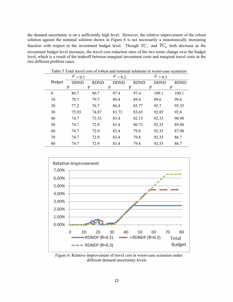
the demand uncertainty is on a sufficiently high level. However, the relative improvement of the robust solution against the nominal solution shown in Figure 6 is not necessarily a monotonically increasing function with respect to the investment budget level. Though rTC and dTC both decrease as the investment budget level increases, the travel cost reduction rates of the two terms change over the budget level, which is a result of the tradeoff between marginal investment costs and marginal travel costs in the two different problem cases.
Table 5 Total travel cost of robust and nominal solutions in worst-case scenarios
Budget θ = 0.1 θ = 0.2 θ = 0.3 DDND
P RDND
P DDND
P RDND
P DDND
P RDND
P 0 86.7 86.7 97.4 97.4 109.1 109.1 10 79.7 79.7 89.4 89.4 99.6 99.6 20 77.2 76.7 86.4 85.77 95.7 95.35 30 75.03 74.87 83.73 83.65 92.85 92.8 40 74.7 73.53 83.4 82.15 92.35 90.98 50 74.7 72.9 83.4 80.73 92.35 89.48 60 74.7 72.9 83.4 79.8 92.35 87.98 70 74.7 72.9 83.4 79.8 92.35 86.7 80 74.7 72.9 83.4 79.8 92.35 86.7
Figure 6: Relative improvement of travel cost in worst-case scenarios under
different demand uncertainty levels

23
Figure 7: Relative improvement of travel cost in worst-case scenarios under
different investment budget levels Next, we fixed the total budget level B at four different levels (including 30, 40, 50 or 60 monetary
units) with the demand uncertainty level θ ranging from 0 to 0.5. The computation result is depicted in Figure 7. We can see that with a lower budget level, the demand uncertainty has a weaker effect on the performance of the RDNDP model. However, the solution of the RDNDP model may be largely different from the solution of the corresponding DDNDP model when the budget level is relatively high. Similar to Figure 6, we can also observe that the relative improvement of the total travel cost of the robust solution against the nominal solution is not always a monotonically increasing function with respect to the demand uncertainty level.
3.5.1.3 Simulation results
Finally, we evaluated the objective function by implementing the robust network design solutions and
nominal solution with random demands generated by the given box uncertainty sets. Specifically, 100 sets of random data generated from a beta distribution (i.e., beta[5, 2]) were used for this evaluation. The mean, standard deviation, and maximum values of the objective function values generated from the simulation experiment are shown and compared in Table 6. It can be seen that, in almost every case, the mean objective function value of the robust solutions is better than that of the nominal solutions; in all cases, the standard deviation and maximum values of the robust solutions are less than or equal to those of the nominal solutions.

24

25
Table 6: Comparison of Simulation Results (a) θ = 0.1
Budget Mean Standard Deviation Maximum DDNDP RDNDP DDNDP RDNDP DDNDP RDNDP
0 80.66 80.66 1.52 1.52 83.55 83.55 10 74.36 74.36 1.27 1.27 77.10 77.10 20 72.01 71.78 1.35 1.29 75.16 74.81 30 70.06 70.18 1.38 1.30 72.78 72.72 40 69.82 68.95 1.07 1.01 72.55 71.55 50 69.62 68.34 1.20 1.07 72.14 70.56 60 69.64 68.35 1.16 1.04 71.88 70.39 70 69.62 68.34 1.09 0.98 71.61 70.02 80 69.64 68.36 1.32 1.18 72.79 71.18
(b) θ = 0.2
Budget Mean Standard Deviation Maximum DDNDP RDNDP DDNDP RDNDP DDNDP RDNDP
0 85.27 85.27 2.96 2.96 93.02 93.02 10 78.22 78.22 2.51 2.51 83.35 83.35 20 76.16 75.69 2.50 2.41 82.14 81.51 30 73.90 73.83 2.47 2.44 78.84 78.76 40 73.56 72.62 2.49 2.34 78.58 77.33 50 73.51 71.49 2.35 2.18 78.82 76.48 60 72.92 70.39 2.68 2.44 77.92 74.89 70 73.41 70.83 2.20 1.96 78.75 75.57 80 73.65 71.05 2.63 2.35 80.03 76.78
(c) θ = 0.3
Budget Mean Standard Deviation Maximum DDNDP RDNDP DDNDP RDNDP DDNDP RDNDP
0 90.21 90.21 4.24 4.24 99.54 99.54 10 82.88 82.88 4.20 4.20 90.37 90.37 20 79.86 79.44 3.64 3.61 87.50 86.97 30 77.30 77.24 3.99 3.98 86.49 86.58 40 77.42 76.34 3.57 3.52 84.98 83.85 50 76.83 74.57 3.45 3.23 84.96 82.33 60 76.88 73.72 3.92 3.57 85.75 81.93 70 76.88 73.72 3.92 3.57 85.75 81.93 80 77.57 73.64 3.52 3.19 84.35 79.85
26
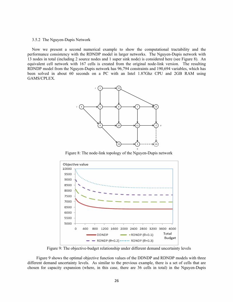
3.5.2 The Nguyen-Dupis Network Now we present a second numerical example to show the computational tractability and the
performance consistency with the RDNDP model in larger networks. The Nguyen-Dupis network with 13 nodes in total (including 2 source nodes and 1 super sink node) is considered here (see Figure 8). An equivalent cell network with 167 cells is created from the original node-link version. The resulting RDNDP model from the Nguyen-Dupis network has 96,794 constraints and 190,694 variables, which has been solved in about 60 seconds on a PC with an Intel 1.87Ghz CPU and 2GB RAM using GAMS/CPLEX.
5 6 74 8
9 10 11 2
13 3
1 12r
r
s
s
14
Figure 8: The node-link topology of the Nguyen-Dupis network
Figure 9: The objective-budget relationship under different demand uncertainty levels
Figure 9 shows the optimal objective function values of the DDNDP and RDNDP models with three
different demand uncertainty levels. As similar to the previous example, there is a set of cells that are chosen for capacity expansion (where, in this case, there are 36 cells in total) in the Nguyen-Dupis
27
network, which delivers a similar objective-budget relationship to the previous toy example. Investment decisions vary with different demand uncertainty levels.
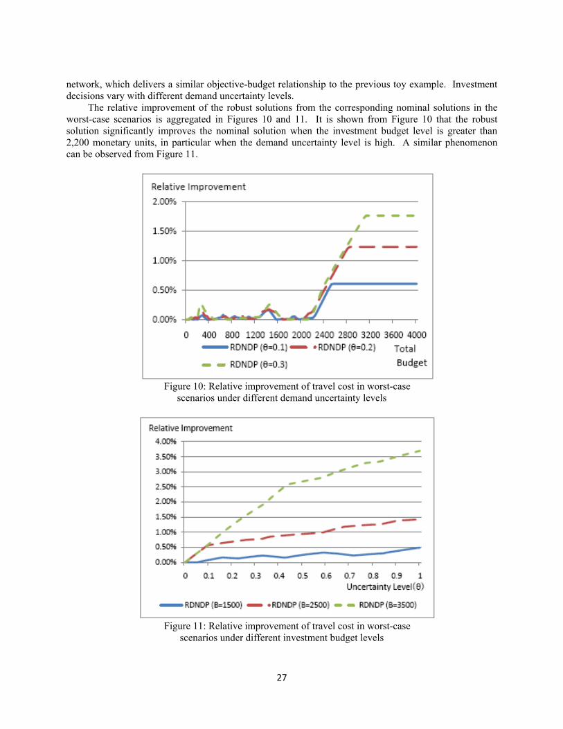
The relative improvement of the robust solutions from the corresponding nominal solutions in the worst-case scenarios is aggregated in Figures 10 and 11. It is shown from Figure 10 that the robust solution significantly improves the nominal solution when the investment budget level is greater than 2,200 monetary units, in particular when the demand uncertainty level is high. A similar phenomenon can be observed from Figure 11.
Figure 10: Relative improvement of travel cost in worst-case
scenarios under different demand uncertainty levels
Figure 11: Relative improvement of travel cost in worst-case
scenarios under different investment budget levels

28
Finally, the simulation results are compared in Table 7. It was found that the simulated objective function values from DDNDP and RDNPD are comparable when the investment budget level is less than 1,500 monetary units. However, the robust solutions provide a lower travel cost when the investment budget goes higher. Our computational results show that the robust solution is more attractive than the nominal solution from the simulation experiment.
Table 7: Comparison of the robust optimization results and simulation results
(a) θ = 0.1
Budget Mean Standard Deviation Maximum DDNDP RDNDP DDNDP RDNDP DDNDP RDNDP
0 7631.63 7631.63 111.42 111.42 7846.08 7846.08 1500 6488.78 6488.61 91.84 91.42 6685.74 6684.25 2500 6391.82 6366.79 78.54 75.08 6549.64 6517.81 3500 6380.82 6353.72 78.88 75.25 6530.00 6497.45
(b) θ = 0.2
Budget Mean Standard Deviation Maximum DDNDP RDNDP DDNDP RDNDP DDNDP RDNDP
0 7976.02 7976.02 204.57 204.57 8395.07 8395.07 1500 6788.14 6784.49 182.44 179.68 7192.98 7185.69 2500 6671.00 6645.71 149.01 143.96 7030.38 6990.74 3500 6666.09 6614.52 154.87 146.25 7006.21 6937.27
(c) θ = 0.3
Budget Mean Standard Deviation Maximum DDNDP RDNDP DDNDP RDNDP DDNDP RDNDP
0 8389.44 8389.44 369.82 369.82 9046.43 9046.43 1500 7096.40 7089.95 272.83 269.47 7847.98 7838.24 2500 6963.85 6931.39 251.54 241.73 7494.99 7441.00 3500 6957.23 6878.45 297.76 278.49 7520.06 7414.78
4. Conclusion
4.1 AARC Conclusions
In Section 2, we applied the RO methodology to the CTM-based SO DTA model under demand uncertainty. In particular, AARC was formulated for dealing with a multi-period transportation problem to find an robust and uncertainty-immunized solution, which is especially important in an emergency logistics problem. Two S-shaped curves with upper and lower bounds were introduced by considering uncertainty sets, which are appropriate for modeling uncertain demand. With the linear decision rule for

29
an approximated solution and the appropriate reformulation technique, AARC becomes a linear programming problem and hence computationally tractable. The objective value obtained is the guaranteed upper bound within a prescribed uncertainty set. Although the AARC solution does not guarantee optimality, we find that the AARC approach leads to high-quality solutions compared to the deterministic problem and the sampling-based stochastic problem.
However, we do not argue that AARC approach always outperforms the stochastic programming. The proposed AARC method is favorable when either reliable information on probability distribution of uncertain parameter is not available or decision makers want to find a strongly guaranteed performance without facing an infeasible solution, even in an extreme case. In those cases, RO can outperform the traditional stochastic programming approach. Also, the purpose of RO is quite different from sensitivity analysis with variation of parameters. RO finds an uncertainty-immunized solution for a pre-described uncertainty set, while sensitivity analysis is a post-optimization tool to test the stability or perturbation of an optimal solution (Ben-Tal and Nemirovski 2000).
Our work has focused on the CTM-based SO-DTA problem by using affine control rule for uncertain demand. The reason for using the linear decision rule is to derive a computationally tractable problem. However, theoretically, we do not know how the approximation makes the robust solution be deviated from the optimal solution. The approximation approach is used based on the belief that it is important to provide a solvable problem in the emergency logistics field (Shapiro and Nemirovski (2005), Remark 2). The scope of future work could be extended to consider control beyond linear decision rule and to explore large scale examples. Moreover, a robust optimization approach can be applied to different uncertainty sources (e.g., capacity uncertainty or cost uncertainty) and alternative transportation problems like dynamic network design.
There are other issues raised from this work. One of these issues is that an LP-based CTM model allows vehicle holding, which may be unrealistic. The RO approach can be applied to alternative deterministic mathematical formulations (e.g., Nie [2010]) to overcome this issue. Extension to considering an unbounded uncertainty set with globalized robust optimization (Ben-Tal et al. 2006) is another interesting research direction.
4.2 RNDP Conclusions
In Section 3, we formulated and solved the RDNDP, a robust network design problem for dynamic and uncertain demands, and numerically evaluated its solution performance. The appealing LP formulation of the RDNDP model is rooted from the underlying LP-based DTA model―CTM. A box uncertainty set is assumed for modeling uncertain demands. Through this NDP example, we demonstrate how the constraints affected by uncertain parameters can be manipulated to derive a tractable mathematical program.
Since it becomes particularly important to provide a solution that is robust to extreme events and reduce the variance of cost after the realization of uncertain parameters (Waller and Ziliaskopoulos 2006), the authors chose a beta distribution (which is an asymmetric distribution) to model random demands and conduct a worst-case analysis. The RO approach can provide better network design solutions that produce lower objective function values than the corresponding deterministic approach, especially at a high demand uncertainty level and a high investment budget level.
Numerous future research directions remain. First, the RDNDP model with various types of uncertainty sets, including a polyhedral uncertainty set or an ellipsoidal uncertainty set, should be investigated to find a less conservative solution. Second, the ambiguous chance-constrained programming can be applied to the model when we have more information about the uncertain data. For example, this approach may be particularly interesting when we only know the support and mean of uncertain parameters or when we know that demand can arise from a set of distributions. Third, while we dealt with the RDNDP with a single-destination, system-optimum network setting, which has potential applications in emergency evacuation planning, optimal traffic detouring, lower-bound evaluation of

30
traffic systems, etc., the user-optimal and multi-destination versions of the same problem are worth further investigation and evaluation along the track of RO.
References
Atamturk, A., and Zhang, M. Two-stage robust network flow and design under demand uncertainty.
Operations Research, 55(4):662-673, 2007.
Ben-Tal, A., and Nemirovski, A. Robust convex optimization. Mathematics of Operations Research
23(4):769-805, 1998.
Ben-Tal, A., and Nemirovski, A. Robust solutions of uncertain linear programs. Operations Research
Letters, 25:1-13, 1999.
Ben-Tal, A., and Nemirovski, A. Robust solutions of linear programming problems contaminated with
uncertain data. Mathematical Programming, 88:411-424, 2000.
Ben-Tal, A., and Nemirovski, A. Robust optimization―methodology and applications. Mathematical
Programming, 92:453-480, 2002.
Ben-Tal, A., El Ghaoui, L., and Nemirovski, A. Robust optimization. Princeton University Press, 2009.
Ben-Tal, A., Goryashko, A., Guslitzer, E., and Nemirovski, A. Adjustable robust solutions of uncertain
linear programs. Mathematical Programming, 99(2):351-376, 2004.
Bertsimas, D., Brown, D. B., and Caramanis, C. Theory and applications of robust optimization. SIAM
Review, 53(3):464-501, 2011.
Bertsimas, D., and Perakis, G. Robust and adaptive optimization: A tractable approach to optimization
under uncertainty. NSF/CMMI/OR 0556106, 2005.
Chiu, Y. C., Zheng, H., Villalobos, J., and Gautam, B. Modeling no-notice mass evacuation using a
dynamic traffic flow optimization model. IIE Transactions, 39(1):83-94, 2007.
Daganzo, C.F. The cell transmission model, part II: Network traffic. Transportation Research Part B,
29(2):79-93, 1995.
Daganzo, C.F. The cell transmission model. part I: A simple dynamic representation of highway traffic.
Transportation Research Part B, 28(2):269-287, 1993.

31
Erera, A. L., Morales, J. C., and Savelsbergh, M. Robust optimization for empty repositioning problems.
Operations Research, 57(2):468-483, 2009.
Friesz, T. L., and Bernstein, D. Handbook of transport modelling, chapter: Analytical dynamic traffic
assignment models, pages 181-195. Pergamon, 2000.
Karoonsoontawong, A., and Waller, S. T. Robust dynamic continuous network design problem.
Transportation Research Record: Journal of the Transportation Research Board, 2029(-1):58-71,
2007.
Lou, Y., Yin, Y., and Lawpongpanich, S. A robust approach to discrete network designs with demand
uncertainty, Transportation Research Record: Journal of the Transportation Research Board,
2090:86-94, 2009.
Lu, Y. Robust transportation network design under user equilibrium, Master’s Thesis, MIT, Cambridge,
MA, 2007.
Magnanti, T. L., and Wong, R. T. Network design and transportation planning: models and algorithms.
Transportation Science, 18(1):1-55, 1984.
Merchant, D. K., and Nemhauser, G. L. A model and an algorithm for the dynamic traffic assignment
problems. Transportation Science, 12(3):183, 1978.
Merchant, D. K., and Nemhauser, G. L. Optimality conditions for a dynamic traffic assignment model.
Transportation Science, 12(3):200, 1978.
Minoux, M. Network synthesis and optimum network design problems: Models, solution methods and
applications. Networks 19(3):313-360, 1989.
Mudchanatongsuk, S. and Ordonez, F. and Liu, J. Robust solutions for network design under
transportation cost and demand uncertainty. Journal of the Operational Research Society, 59(5):652-
662, 2008.
Mulvey, J. M., Vanderbei, R. J., and Zenios, S. A. Robust optimization of large-scale systems.
Operations Research, 43(2):264-281, 1995.
Nie, Y. A Cell-based Merchant-Nemhauser Model for the System Optimum Dynamic Traffic
Assignment Problem. Transportation Research Part B, 45(2):329-342, 2011.

32
Ordóñez, F. and Zhao, J. Robust capacity expansion of network flows. Networks, 50(2):136-145, 2007.
Peeta, S., and Zhou, C. Robustness of the off-line a priori stochastic dynamic traffic assignment solution
for on-line operations. Transportation Research Part C, 7(5):281-303, 1999.
Peeta, S., and Ziliaskopoulos, A. K. Foundations of dynamic traffic assignment: The past, the present
and the future. Networks and Spatial Economics, 1(3):233-265, 2001.
Shapiro, A., and Nemirovski, A. On complexity of stochastic programming problems. Continuous
Optimization, 99:11-146, 2005.
Tuydes, H. Network traffic management under disaster conditions. PhD thesis, Northwestern
University, Evanston, IL., 2005.
Ukkusuri, S. V., and Waller, S. T. Linear programming models for the user and system optimal dynamic
network design problem: formulations, comparisons and extensions. Networks and Spatial
Economics, 8(4):383-406, 2008.
Ukkusuri, S. V., Mathew, T., and Waller, T. Robust transportation network design under demand
uncertainty. Computer-Aided Civil and Infrastructure Engineering 22(1):6-18, 2007.
Waller, S. T., Schofer, J. L., and Ziliaskopoulos, A. K. Evaluation with traffic assignment under demand
uncertainty. Transportation Research Record: Journal of the Transportation Research Board,
1771:69-74, 2001.
Waller, S. T., and Ziliaskopoulos, A.K. Stochastic dynamic network design problem. Transportation
Research Record: Journal of the Transportation Research Board, 1771:106-113, 2001.
Waller, S. T., and Ziliaskopoulos, A. K. A chance-constrained based stochastic dynamic traffic
assignment model: Analysis, formulation and solution algorithms. Transportation Research Part C,
14(6):418-427, 2006.
Xie, C., Lin, D. Y., and Travis Waller, S. A dynamic evacuation network optimization problem with
lane reversal and crossing elimination strategies. Transportation Research Part E, 46(3):295-316,
2010.
Yang, H., and Bell, M. G. H. Models and algorithms for road network design: a review and some new
developments. Transport Reviews, 18(3):257–278, 1998.

33
Yao, T., Mandala, S. R., and Chung, B. D. Evacuation transportation planning under uncertainty: A
robust optimization approach. Networks and Spatial Economics, 9:171-189, 2009.
Yazici, M. A., and Ozbay, K. Impact of Probabilistic Road Capacity Constraints on the Spatial
Distribution of Hurricane Evacuation Shelter Capacities. Transportation Research Record: Journal of
the Transportation Research Board, 2022:55-62, 2007.
Yin, Y., Lawphongpanich, S., and Lou, Y. Estimating investment requirement for maintaining and
improving highway systems. Transportation Research Part C, 16(2):199-211, 2008.
Yin, Y., Madanat, S. M., and Lu, X. Y. Robust improvement schemes for road networks under demand
uncertainty. European Journal of Operational Research, 198(2):470-479, 2009.
Zhao, Y., and Kockelman, K. The propagation of uncertainty through travel demand models: An
exploratory analysis. Annals of Regional Science, 36(1):145-163, 2002.
Ziliaskopoulos, A. K. A linear programming model for the single destination system optimum dynamic
traffic assignment problem. Transportation Science, 34(1):37-49, 2000.