robust wireless sensor network for smart grid

Robust Wireless Sensor Network for Smart GridCommunication: Modeling and Performance Evaluation

by

Md Sahabul ALAM

MANUSCRIPT-BASED THESIS PRESENTED TO ÉCOLE DE

TECHNOLOGIE SUPÉRIEURE

IN PARTIAL FULFILLMENT FOR THE DEGREE OF

DOCTOR OF PHILOSOPHY

Ph.D.

MONTREAL, AUGUST 1ST, 2019

ÉCOLE DE TECHNOLOGIE SUPÉRIEUREUNIVERSITÉ DU QUÉBEC

Md. Sahabul Alam, 2019

This Creative Commons license allows readers to download this work and share it with others as long as the

author is credited. The content of this work cannot be modified in any way or used commercially.

BOARD OF EXAMINERS

THIS THESIS HAS BEEN EVALUATED

BY THE FOLLOWING BOARD OF EXAMINERS

Professor Georges Kaddoum, Thesis Supervisor

Department of Electrical Engineering, École de Technologie Supérieure

Dr. Basile L. Agba, Co-supervisor

Hydro-Quebec Research Institute (IREQ)

Professor Mohamed Faten Zhani, President of the Board of Examiners

Department of Software and IT Engineering, École de Technologie Supérieure

Professor Eric Granger, Member of the jury

Department of Automated Manufacturing Engineering, École de Technologie Supérieure

Professor Tareq Al-Naffouri, External Independent Examiner

KAUST, Saudi Arabia

THIS THESIS WAS PRESENTED AND DEFENDED

IN THE PRESENCE OF A BOARD OF EXAMINERS AND THE PUBLIC

ON JULY 24, 2019

AT ÉCOLE DE TECHNOLOGIE SUPÉRIEURE

V

To my mother, because of whom I am here

My wife and two loving kids

And my brothers, sisters and other family members

FOREWORD

This dissertation is mainly based on the research outcomes, which are accomplished under the

supervision of Dr. Georges Kaddoum from May 2016 to Jul. 2019. This work is financially

supported by the FRQNT and NSERC Ph.D. fellowships. This dissertation is subjective to

address the wireless sensor network based reliable communication for smart grid environments.

Resultantly, my Ph.D. study successfully ended with 4 journal paper published, 1 journal paper

under review and 1 journal paper prepared for submission as the first author, and co-authored

6 journals.

Apart from the first two chapters, where the background of smart grid communications are

intensively introduced, the remaining chapters are based on my journal papers. For those chap-

ters, I did a comprehensive literature review, reasonably formulated problems, feasibly pro-

posed possible solutions, mathematically analyzed and simulated the performance, and tech-

nically drafted manuscripts. After the presentation of those chapters, chapter 7 concludes the

whole work and list several future research directions.

ACKNOWLEDGEMENTS

First and foremost, I would like to show my sincere gratitude to my supervisor Dr. Georges

Kaddoum for his considerate guidance, valuable inspiration, constructive suggestion, and con-

sistent encouragement throughout my three and half years research study. This thesis would

not come to the completion without his dedicated mentor and scholarly inputs.

Besides my supervisor, I am also appreciative to Dr. Basile L. Agba (senior scientist, Hydro-

Quebec Research Institute (IREQ)) who serves as my co-supervisor. Similar profound grati-

tude also goes to Professor Eric Granger, Professor Mohamed Faten Zhani, and Professor Tareq

Al-Naffouri for their agreement to serve as my jury members. Each of the members of my Dis-

sertation Committee has provided me extensive personal and professional guidance and taught

me a great deal about both scientific research and life in general. Also, a special mention and

thanks goes to the FRQNT and NSERC postgraduate fellowship programs for their financial

support during my Ph.D. study.

I am grateful to all of those with whom I have had the pleasure to work during this and other

related projects. Many thanks also goes to my friends for their help to encourage me with high

enthusiasm to embrace my research problems. I do hereby acknowledge all my colleagues

from LACIME group, including Khaled, Bassant, Victor, Dawa, Zeeshan, Elli, Hamza, Long,

Vu, Jung, Michael, Nancy, Ibrahim, Marwan, Dat, etc., and my ETS friends including Hashem,

Mahmud, Rizwan, Adel, and Abu.

Nobody has been more patient in the pursuit of this project than the members of my family. I

would like to thank my loving and supportive wife, Fatema Khatun who keep me away from

depression, and my two wonderful children, Safin and Sayam, who sacrificed a lot and provided

unending inspiration.

Finally, I would like to wholeheartedly thank my mother for her continued patience, uncondi-

tional support, and warm love. In particularly, I owe my mother my deepest apology since I

was not with her since long time in her old age. I born in a small village of a developing Coun-

X

try and She is the person for whom I am here. I feel sorry for my departed father who straggled

all his life to make us happy and he can not share this biggest joy. Also, my special thanks

and appreciation to my sisters, brothers, nephews, and nieces for their spiritually invaluable

support and love to my studies and life.

Réseau de capteurs sans fil robuste pour la communication sur réseau intelligent :Modélisation et évaluation du rendement

Md Sahabul ALAM

RÉSUMÉ

Notre planète se dirige progressivement vers une famine énergétique due à la croissance dé-

mographique et à l’industrialisation. Par conséquent, l’augmentation de la consommation et

des prix de l’électricité, la diminution des combustibles fossiles et le manque de protection de

l’environnement par les émissions de gaz à effet de serre, ainsi que l’utilisation inefficace des

approvisionnements énergétiques existants ont provoqué ces dernières années des problèmes

graves de congestion des réseaux dans de nombreux pays. En plus de cette situation de sur-

charge, le système électrique est aujourd’hui confronté à de nombreux défis, tels que les coûts

de maintenance élevés, le vieillissement des équipements, l’absence de diagnostic efficace des

pannes, la fiabilité de l’alimentation électrique, etc. qui augmentent encore les risques de

panne du système. En outre, l’adaptation des nouvelles sources d’énergie renouvelables avec

les centrales électriques existantes, pour offrir une alternative à la production d’électricité, l’a

transformée en une échelle très vaste et complexe, ce qui soulève de nouveaux problèmes.

Pour relever ces défis, un nouveau concept de réseau électrique de la prochaine génération,

appelé "réseau intelligent", a vu le jour, dans lequel les technologies de l’information et de la

communication (TIC) jouent un rôle clé. Pour un réseau intelligent fiable, la surveillance et le

contrôle des paramètres du réseau électrique dans les segments de transport et de distribution

sont essentiels. Cela nécessite le déploiement d’un réseau de communication robuste au sein

du réseau électrique. Traditionnellement, les communications sur le réseau électrique sont réal-

isées au moyen de communications câblées, y compris les communications par ligne électrique

(PLC). Cependant, le coût de son installation peut s’avérer onéreux, en particulier pour les ap-

plications de contrôle et de surveillance à distance. Plus récemment, de nombreux intérêts de

recherche ont été attirés par les communications sans fil pour les applications de réseaux intel-

ligents. A cet égard, les méthodes les plus prometteuses de surveillance des réseaux intelligents

explorées dans la littérature sont basées sur les réseaux de capteurs sans fil (WSN). En effet, la

nature collaborative du WSN apporte des avantages significatifs par rapport aux réseaux sans

fil traditionnels, y compris une couverture plus large et à faible coût, une auto-organisation et

un déploiement rapide. Malheureusement, les environnements rudes et hostiles des systèmes

d’alimentation électrique posent de grands défis pour la fiabilité des communications entre les

nœuds de capteurs en raison des fortes interférences radiofréquence et du bruit appelé "bruit

impulsif".

En raison de l’importance fondamentale des communications sur réseau intelligent basées sur

WSN et de l’impact possible du bruit impulsif sur la fiabilité des communications des nœuds de

capteurs, cette thèse est censée combler le manque dans les résultats des recherches existants.

Pour être plus précis, les contributions de cette thèse peuvent être résumées en trois volets : (i)

l’étude et l’analyse des performances des techniques d’atténuation du bruit impulsionnel pour

les systèmes de communication à porteuse unique point-à-point altérés par un bruit impulsion-

XII

nel en rafale ; (ii) la conception et l’analyse des performances des réseaux WSN collaboratifs

pour la communication intelligente en tenant compte du modèle de bruit RF dans le proces-

sus de conception, une intention particulière est donnée à la manière de prendre en compte la

corrélation dans le temps des échantillons de bruit ; (iii) estimation par erreur carrée moyenne

minimale optimale (EMM) des phénomènes physiques comme la température, l’intensité et la

tension, typiquement modélisé par une source gaussienne en présence d’un bruit impulsif.

Dans la première partie, nous comparons et analysons les méthodes non linéaires largement

utilisées telles que l’écrêtage, l’effacement et la combinaison écrêtage/effacement pour at-

ténuer les effets nocifs du bruit impulsionnel en rafale dans les systèmes de communication

point à point avec transmission mono-porteuse à codage LDPC (Low-Density Parity Check).

Bien que la performance de ces techniques d’atténuation soit largement étudiée pour les sys-

tèmes de communication multi-porteuses utilisant le multiplexage par répartition en fréquence

orthogonale (OFDM) sous l’effet du bruit impulsif sans mémoire, on constate que le OFDM

est moins performant que sa homologue mono-porteuse lorsque les impulsions sont très fortes

et/ou fréquentes, comme on peut en retrouver dans les systèmes de communication actuels,

dont les réseaux de communications de grilles intelligentes. De même, l’hypothèse d’un mod-

èle de bruit sans mémoire n’est pas valable pour de nombreux scénarios de communication. De

plus, nous proposons une atténuation du bruit impulsif basée sur le logarithme du rapport de

vraisemblance (LLR) pour le scénario considéré. Nous montrons que la propriété de mémoire

du bruit peut être exploitée dans le calcul du LLR par une détection maximale à posteriori

(MAP). Dans ce contexte, les résultats de simulation fournis mettent en évidence la supériorité

du système d’atténuation basé sur les LLR par rapport aux simples systèmes de coupures par

écrêtage/effacement.

La deuxième contribution peut être divisée en deux volets : (i) nous considérons l’analyse

des performances d’un système de relais coopératif de décodage et de transmission (DF) à

relais simple, sur des canaux altérés par un bruit impulsionnel en rafale. Pour ce canal, les

performances du taux d’erreur binaire (TEB) de la transmission directe et d’un schéma de

relais DF utilisant la modulation M-PSK en présence d’évanouissements de Rayleigh avec un

récepteur MAP sont dérivées ; (ii) dans le prolongement du schéma WSN collaboratif simple

relais, nous proposons un nouveau protocole de sélection de relais pour un WSN collectif DF

multi relais prenant en compte le bruit impulsionnel en rafale. Le protocole proposé choisit le

meilleur relais N’th en tenant compte à la fois des gains de canal et des états du bruit impulsif

des liaisons relais source-relais et relais-destination. Pour analyser la performance du protocole

proposé, nous dérivons d’abord des expressions de forme analytique exacte pour la fonction

de densité de probabilité (PDF) du SNR reçu. Ensuite, ces PDFs sont utilisés pour dériver des

expressions de forme analytique exactes pour le TEB et la probabilité d’interruption. Enfin,

nous dérivons également les expressions asymptotiques du TEB et des coupures pour quantifier

les avantages de la diversité. Les résultats obtenus montrent que les récepteurs proposés sur

la base du critère de détection MAP sont les plus appropriés pour les environnements de bruit

impulsionnel en rafales car ils ont été conçus en fonction du comportement statistique du bruit.

XIII

A la différence des contributions susmentionnées, nous avons parlé de la détection fiable des

alphabets finis en présence d’un bruit impulsif en rafale, dans la troisième partie, nous étudions

l’estimation MMSE optimale pour une source gaussienne scalaire altérée par un bruit impul-

sif. Au chapitre 5, l’estimation bayésienne optimale du MMSE pour une source gaussienne

scalaire, en présence d’un bruit impulsionnel en rafale, est examinée. D’autre part, au chapitre

6, nous étudions l’estimation distribuée d’une source gaussienne scalaire dans les WSNs en

présence d’un bruit de classe A de Middleton. D’après les résultats obtenus, nous concluons

que l’estimateur MMSE optimal proposé surpasse l’estimateur MMSE linéaire développé pour

le canal gaussien.

Mots-clés: : Communication sur réseau de grille intelligente, réseau de capteurs sans fil, bruit

impulsif, communication coopérative, détection a posteriori maximale, estimation de l’erreur

carrée moyenne minimale.

Robust Wireless Sensor Network for Smart Grid Communication: Modeling andPerformance Evaluation

Md Sahabul ALAM

ABSTRACT

Our planet is gradually heading towards an energy famine due to growing population and in-

dustrialization. Hence, increasing electricity consumption and prices, diminishing fossil fuels

and lack significantly in environment-friendliness due to their emission of greenhouse gasses,

and inefficient usage of existing energy supplies have caused serious network congestion prob-

lems in many countries in recent years. In addition to this overstressed situation, nowadays, the

electric power system is facing many challenges, such as high maintenance cost, aging equip-

ment, lack of effective fault diagnostics, power supply reliability, etc., which further increase

the possibility of system breakdown. Furthermore, the adaptation of the new renewable energy

sources with the existing power plants to provide an alternative way for electricity production

transformed it in a very large and complex scale, which increases new issues. To address these

challenges, a new concept of next generation electric power system, called the "smart grid",

has emerged in which Information and Communication Technologies (ICTs) are playing the

key role.

For a reliable smart grid, monitoring and control of power system parameters in the trans-

mission and distribution segments are crucial. This necessitates the deployment of a robust

communication network within the power grid. Traditionally, power grid communications are

realized through wired communications, including power line communication (PLC). How-

ever, the cost of its installation might be expensive especially for remote control and monitoring

applications. More recently, plenty of research interests have been drawn to the wireless com-

munications for smart grid applications. In this regard, the most promising methods of smart

grid monitoring explored in the literature is based on wireless sensor network (WSN). Indeed,

the collaborative nature of WSN brings significant advantages over the traditional wireless

networks, including low-cost, wider coverage, self-organization, and rapid deployment. Un-

fortunately, harsh and hostile electric power system environments pose great challenges in the

reliability of sensor node communications because of strong RF interference and noise called

impulsive noise.

On account of the fundamental of WSN-based smart grid communications and the possible

impacts of impulsive noise on the reliability of sensor node communications, this dissertation

is supposed to further fill the lacking of the existing research outcomes. To be specific, the

contributions of this dissertation can be summarized as three fold: (i) investigation and per-

formance analysis of impulsive noise mitigation techniques for point-to-point single-carrier

communication systems impaired by bursty impulsive noise; (ii) design and performance anal-

ysis of collaborative WSN for smart grid communication by considering the RF noise model

in the designing process, a particular intension is given to how the time-correlation among the

noise samples can be taken into account; (iii) optimal minimum mean square error (MMSE)

XVI

estimation of physical phenomenon like temperature, current, voltage, etc., typically modeled

by a Gaussian source in the presence of impulsive noise.

In the first part, we compare and analyze the widely used non-linear methods such as clipping,

blanking, and combined clipping-blanking to mitigate the noxious effects of bursty impul-

sive noise for point-to-point communication systems with low-density parity-check (LDPC)

coded single-carrier transmission. While, the performance of these mitigation techniques are

widely investigated for multi-carrier communication systems using orthogonal frequency divi-

sion multiplexing (OFDM) transmission under the effect of memoryless impulsive noise, we

note that OFDM is outperformed by its single-carrier counterpart when the impulses are very

strong and/or they occur frequently, which likely exists in contemporary communication sys-

tems including smart grid communications. Likewise, the assumption of memoryless noise

model is not valid for many communication scenarios. Moreover, we propose log-likelihood

ratio (LLR)-based impulsive noise mitigation for the considered scenario. We show that the

memory property of the noise can be exploited in the LLR calculation through maximum a pos-

teriori (MAP) detection. In this context, provided simulation results highlight the superiority

of the LLR-based mitigation scheme over the simple clipping/blanking schemes.

The second contribution can be divided into two aspects: (i) we consider the performance

analysis of a single-relay decode-and-forward (DF) cooperative relaying scheme over channels

impaired by bursty impulsive noise. For this channel, the bit error rate (BER) performances

of direct transmission and a DF relaying scheme using M-PSK modulation in the presence of

Rayleigh fading with a MAP receiver are derived; (ii) as a continuation of single-relay collab-

orative WSN scheme, we propose a novel relay selection protocol for a multi-relay DF collab-

orative WSN taking into account the bursty impulsive noise. The proposed protocol chooses

the N’th best relay considering both the channel gains and the states of the impulsive noise

of the source-relay and relay-destination links. To analyze the performance of the proposed

protocol, we first derive closed-form expressions for the probability density function (PDF) of

the received SNR. Then, these PDFs are used to derive closed-form expressions for the BER

and the outage probability. Finally, we also derive the asymptotic BER and outage expres-

sions to quantify the diversity benefits. From the obtained results, it is seen that the proposed

receivers based on the MAP detection criterion is the most suitable one for bursty impulsive

noise environments as it has been designed according to the statistical behavior of the noise.

Different from the aforementioned contributions, talked about the reliable detection of finite

alphabets in the presence of bursty impulsive noise, in the thrid part, we investigate the optimal

MMSE estimation for a scalar Gaussian source impaired by impulsive noise. In Chapter 5,

the MMSE optimal Bayesian estimation for a scalar Gaussian source, in the presence of bursty

impulsive noise is considered. On the other hand, in Chapter 6, we investigate the distributed

estimation of a scalar Gaussian source in WSNs in the presence of Middleton class-A noise.

From the obtained results we conclude that the proposed optimal MMSE estimator outperforms

the linear MMSE estimator developed for Gaussian channel.

XVII

Keywords: Smart grid communication, wireless sensor network, impulsive noise, cooperative

communication, maximum a posteriori detection, minimum mean square error estimation.

TABLE OF CONTENTS

Page

INTRODUCTION . . . . . . . . . . . . . . . . . . . . . . . . . . . . . . . . . . . . . . . . . . . . . . . . . . . . . . . . . . . . . . . . . . . . . . . . . . . . . . . . 1

CHAPTER 1 BACKGROUND AND LITERATURE REVIEW .. . . . . . . . . . . . . . . . . . . . . . . . 13

1.1 What is Smart Grid? . . . . . . . . . . . . . . . . . . . . . . . . . . . . . . . . . . . . . . . . . . . . . . . . . . . . . . . . . . . . . . . . . . . . 13

1.2 Smart Grid Communications . . . . . . . . . . . . . . . . . . . . . . . . . . . . . . . . . . . . . . . . . . . . . . . . . . . . . . . . . . . 14

1.2.1 Power Line Communication . . . . . . . . . . . . . . . . . . . . . . . . . . . . . . . . . . . . . . . . . . . . . . . . . . 16

1.2.2 Satellite Communication . . . . . . . . . . . . . . . . . . . . . . . . . . . . . . . . . . . . . . . . . . . . . . . . . . . . . 17

1.2.3 Optical Fiber Communication . . . . . . . . . . . . . . . . . . . . . . . . . . . . . . . . . . . . . . . . . . . . . . . . 17

1.2.4 Wireless Communications . . . . . . . . . . . . . . . . . . . . . . . . . . . . . . . . . . . . . . . . . . . . . . . . . . . . 18

1.2.4.1 Cellular Communications . . . . . . . . . . . . . . . . . . . . . . . . . . . . . . . . . . . . . . . . . 18

1.2.4.2 ZigBee Network . . . . . . . . . . . . . . . . . . . . . . . . . . . . . . . . . . . . . . . . . . . . . . . . . . . 19

1.2.4.3 WLAN . . . . . . . . . . . . . . . . . . . . . . . . . . . . . . . . . . . . . . . . . . . . . . . . . . . . . . . . . . . . . 20

1.3 WSN Applications in Smart Grid Communications . . . . . . . . . . . . . . . . . . . . . . . . . . . . . . . . . . . 21

1.4 Characteristics of WSN . . . . . . . . . . . . . . . . . . . . . . . . . . . . . . . . . . . . . . . . . . . . . . . . . . . . . . . . . . . . . . . . . 23

1.4.1 Basic Structure of WSNs . . . . . . . . . . . . . . . . . . . . . . . . . . . . . . . . . . . . . . . . . . . . . . . . . . . . . 23

1.4.2 Sensor Node Components . . . . . . . . . . . . . . . . . . . . . . . . . . . . . . . . . . . . . . . . . . . . . . . . . . . . 24

1.4.3 Benefits of WSNs for Smart Grid Automation . . . . . . . . . . . . . . . . . . . . . . . . . . . . . . 25

1.5 Design Challenges of WSNs in Smart Grids . . . . . . . . . . . . . . . . . . . . . . . . . . . . . . . . . . . . . . . . . . 26

1.6 Impulsive Noise . . . . . . . . . . . . . . . . . . . . . . . . . . . . . . . . . . . . . . . . . . . . . . . . . . . . . . . . . . . . . . . . . . . . . . . . . 29

1.6.1 Middleton Class-A Model . . . . . . . . . . . . . . . . . . . . . . . . . . . . . . . . . . . . . . . . . . . . . . . . . . . . 32

1.6.2 Bernoulli-Gaussian Model . . . . . . . . . . . . . . . . . . . . . . . . . . . . . . . . . . . . . . . . . . . . . . . . . . . . 34

1.6.3 Two-state Markov-Gaussian Model . . . . . . . . . . . . . . . . . . . . . . . . . . . . . . . . . . . . . . . . . . 37

1.6.4 Zimmermann Model . . . . . . . . . . . . . . . . . . . . . . . . . . . . . . . . . . . . . . . . . . . . . . . . . . . . . . . . . . 39

1.6.5 Markov-Middleton Model . . . . . . . . . . . . . . . . . . . . . . . . . . . . . . . . . . . . . . . . . . . . . . . . . . . . 40

1.7 Impulsive Noise Mitigation Techniques . . . . . . . . . . . . . . . . . . . . . . . . . . . . . . . . . . . . . . . . . . . . . . . 42

1.7.1 Conventional Impulsive Noise Mitigation Techniques . . . . . . . . . . . . . . . . . . . . . . 42

1.7.1.1 Clipping . . . . . . . . . . . . . . . . . . . . . . . . . . . . . . . . . . . . . . . . . . . . . . . . . . . . . . . . . . . 42

1.7.1.2 Blanking . . . . . . . . . . . . . . . . . . . . . . . . . . . . . . . . . . . . . . . . . . . . . . . . . . . . . . . . . . . 42

1.7.1.3 Combined Clipping-Blanking . . . . . . . . . . . . . . . . . . . . . . . . . . . . . . . . . . . . 43

1.7.2 LLR-based Mitigation . . . . . . . . . . . . . . . . . . . . . . . . . . . . . . . . . . . . . . . . . . . . . . . . . . . . . . . . 44

1.7.2.1 LLR Calculation for Memoryless Impulsive Noise: . . . . . . . . . . . . 45

1.7.2.2 LLR Calculation for Impulsive Noise with memory . . . . . . . . . . . . 45

1.8 Cooperative Communication . . . . . . . . . . . . . . . . . . . . . . . . . . . . . . . . . . . . . . . . . . . . . . . . . . . . . . . . . . . 48

1.8.1 Cooperative Communication Protocols . . . . . . . . . . . . . . . . . . . . . . . . . . . . . . . . . . . . . . 49

1.8.2 Types of Combining . . . . . . . . . . . . . . . . . . . . . . . . . . . . . . . . . . . . . . . . . . . . . . . . . . . . . . . . . . 51

1.8.3 Cooperative Communications over Impulsive Noise Channels . . . . . . . . . . . . . 52

CHAPTER 2 MITIGATION TECHNIQUES FOR IMPULSIVE NOISE WITH

MEMORY . . . . . . . . . . . . . . . . . . . . . . . . . . . . . . . . . . . . . . . . . . . . . . . . . . . . . . . . . . . . . . . . . . . . 59

2.1 Abstract . . . . . . . . . . . . . . . . . . . . . . . . . . . . . . . . . . . . . . . . . . . . . . . . . . . . . . . . . . . . . . . . . . . . . . . . . . . . . . . . . . 59

XX

2.2 Introduction . . . . . . . . . . . . . . . . . . . . . . . . . . . . . . . . . . . . . . . . . . . . . . . . . . . . . . . . . . . . . . . . . . . . . . . . . . . . . . 60

2.3 System Model . . . . . . . . . . . . . . . . . . . . . . . . . . . . . . . . . . . . . . . . . . . . . . . . . . . . . . . . . . . . . . . . . . . . . . . . . . . 65

2.3.1 Signal Model . . . . . . . . . . . . . . . . . . . . . . . . . . . . . . . . . . . . . . . . . . . . . . . . . . . . . . . . . . . . . . . . . . 65

2.3.2 The Two-state Markov-Gaussian Model . . . . . . . . . . . . . . . . . . . . . . . . . . . . . . . . . . . . . 66

2.4 Impulsive Noise Mitigation Techniques . . . . . . . . . . . . . . . . . . . . . . . . . . . . . . . . . . . . . . . . . . . . . . . 68

2.4.1 Conventional Impulsive Noise Mitigation Techniques . . . . . . . . . . . . . . . . . . . . . . 68

2.4.1.1 Clipping . . . . . . . . . . . . . . . . . . . . . . . . . . . . . . . . . . . . . . . . . . . . . . . . . . . . . . . . . . . 68

2.4.1.2 Blanking . . . . . . . . . . . . . . . . . . . . . . . . . . . . . . . . . . . . . . . . . . . . . . . . . . . . . . . . . . . 68

2.4.1.3 Combined Clipping-Blanking . . . . . . . . . . . . . . . . . . . . . . . . . . . . . . . . . . . . 69

2.4.1.4 Optimal Threshold Determination for the Non-

Linearity . . . . . . . . . . . . . . . . . . . . . . . . . . . . . . . . . . . . . . . . . . . . . . . . . . . . . . . . . . . 70

2.4.2 LLR-based Mitigation . . . . . . . . . . . . . . . . . . . . . . . . . . . . . . . . . . . . . . . . . . . . . . . . . . . . . . . . 74

2.4.2.1 LLR Calculation for Memoryless Impulsive Noise: . . . . . . . . . . . . 75

2.4.2.2 LLR Calculation for Impulsive Noise with memory . . . . . . . . . . . . 75

2.5 Performances Evaluation . . . . . . . . . . . . . . . . . . . . . . . . . . . . . . . . . . . . . . . . . . . . . . . . . . . . . . . . . . . . . . . 78

2.6 Exact LLR Derivation when using a Non-linearity . . . . . . . . . . . . . . . . . . . . . . . . . . . . . . . . . . . . 82

2.7 Conclusion . . . . . . . . . . . . . . . . . . . . . . . . . . . . . . . . . . . . . . . . . . . . . . . . . . . . . . . . . . . . . . . . . . . . . . . . . . . . . . . 83

CHAPTER 3 PERFORMANCE ANALYSIS OF DF COOPERATIVE RELAYING

OVER BURSTY IMPULSIVE NOISE CHANNEL . . . . . . . . . . . . . . . . . . . . . . . 85

3.1 Abstract . . . . . . . . . . . . . . . . . . . . . . . . . . . . . . . . . . . . . . . . . . . . . . . . . . . . . . . . . . . . . . . . . . . . . . . . . . . . . . . . . . 85

3.2 Introduction . . . . . . . . . . . . . . . . . . . . . . . . . . . . . . . . . . . . . . . . . . . . . . . . . . . . . . . . . . . . . . . . . . . . . . . . . . . . . . 86

3.3 System model . . . . . . . . . . . . . . . . . . . . . . . . . . . . . . . . . . . . . . . . . . . . . . . . . . . . . . . . . . . . . . . . . . . . . . . . . . . 90

3.4 An overview of two-state Markov-Gaussian model . . . . . . . . . . . . . . . . . . . . . . . . . . . . . . . . . . . 93

3.5 Performance analysis . . . . . . . . . . . . . . . . . . . . . . . . . . . . . . . . . . . . . . . . . . . . . . . . . . . . . . . . . . . . . . . . . . . 95

3.5.1 Maximum a Posteriori (MAP) Detection . . . . . . . . . . . . . . . . . . . . . . . . . . . . . . . . . . . . 95

3.5.2 BER of Direct Transmission . . . . . . . . . . . . . . . . . . . . . . . . . . . . . . . . . . . . . . . . . . . . . . . . . 98

3.5.3 BER of DF Cooperative Relaying . . . . . . . . . . . . . . . . . . . . . . . . . . . . . . . . . . . . . . . . . . .100

3.6 Numerical results . . . . . . . . . . . . . . . . . . . . . . . . . . . . . . . . . . . . . . . . . . . . . . . . . . . . . . . . . . . . . . . . . . . . . . .104

3.7 Conclusion . . . . . . . . . . . . . . . . . . . . . . . . . . . . . . . . . . . . . . . . . . . . . . . . . . . . . . . . . . . . . . . . . . . . . . . . . . . . . .113

CHAPTER 4 A NOVEL RELAY SELECTION STRATEGY OF COOPERATIVE

NETWORK IMPAIRED BY BURSTY IMPULSIVE NOISE . . . . . . . . . . .115

4.1 Abstract . . . . . . . . . . . . . . . . . . . . . . . . . . . . . . . . . . . . . . . . . . . . . . . . . . . . . . . . . . . . . . . . . . . . . . . . . . . . . . . . .115

4.2 Introduction . . . . . . . . . . . . . . . . . . . . . . . . . . . . . . . . . . . . . . . . . . . . . . . . . . . . . . . . . . . . . . . . . . . . . . . . . . . . .116

4.3 System Model . . . . . . . . . . . . . . . . . . . . . . . . . . . . . . . . . . . . . . . . . . . . . . . . . . . . . . . . . . . . . . . . . . . . . . . . . .121

4.3.1 Signal Model . . . . . . . . . . . . . . . . . . . . . . . . . . . . . . . . . . . . . . . . . . . . . . . . . . . . . . . . . . . . . . . . .122

4.3.2 Noise Model . . . . . . . . . . . . . . . . . . . . . . . . . . . . . . . . . . . . . . . . . . . . . . . . . . . . . . . . . . . . . . . . . .123

4.4 Relay Selection Protocols . . . . . . . . . . . . . . . . . . . . . . . . . . . . . . . . . . . . . . . . . . . . . . . . . . . . . . . . . . . . . .124

4.4.1 Conventional Best Relay Selection Protocol . . . . . . . . . . . . . . . . . . . . . . . . . . . . . . .124

4.4.2 Proposed Relay Selection Protocol in the Presence of Bursty

Impulsive Noise . . . . . . . . . . . . . . . . . . . . . . . . . . . . . . . . . . . . . . . . . . . . . . . . . . . . . . . . . . . . . .124

4.4.2.1 Genie detection . . . . . . . . . . . . . . . . . . . . . . . . . . . . . . . . . . . . . . . . . . . . . . . . . . .127

4.4.2.2 Proposed MAP based state detection algorithm . . . . . . . . . . . . . . . .127

XXI

4.4.2.3 Memoryless state detection . . . . . . . . . . . . . . . . . . . . . . . . . . . . . . . . . . . . . .128

4.4.3 Random Relay Selection Protocol . . . . . . . . . . . . . . . . . . . . . . . . . . . . . . . . . . . . . . . . . .130

4.4.4 Complexity Discussion . . . . . . . . . . . . . . . . . . . . . . . . . . . . . . . . . . . . . . . . . . . . . . . . . . . . . .130

4.5 BER Performance Analysis . . . . . . . . . . . . . . . . . . . . . . . . . . . . . . . . . . . . . . . . . . . . . . . . . . . . . . . . . . . .130

4.5.1 Calculation of Pe,D(N) . . . . . . . . . . . . . . . . . . . . . . . . . . . . . . . . . . . . . . . . . . . . . . . . . . . . . . .131

4.5.1.1 BER analysis at the N’th best relay . . . . . . . . . . . . . . . . . . . . . . . . . . . . .131

4.5.1.2 BER analysis at the destination . . . . . . . . . . . . . . . . . . . . . . . . . . . . . . . . .133

4.5.2 Calculation of PBe,D . . . . . . . . . . . . . . . . . . . . . . . . . . . . . . . . . . . . . . . . . . . . . . . . . . . . . . . . . . .135

4.6 Outage analysis . . . . . . . . . . . . . . . . . . . . . . . . . . . . . . . . . . . . . . . . . . . . . . . . . . . . . . . . . . . . . . . . . . . . . . . . .136

4.6.1 Calculation of Pout(N) . . . . . . . . . . . . . . . . . . . . . . . . . . . . . . . . . . . . . . . . . . . . . . . . . . . . . . .137

4.6.2 Calculation of PBout . . . . . . . . . . . . . . . . . . . . . . . . . . . . . . . . . . . . . . . . . . . . . . . . . . . . . . . . . . .138

4.7 Asymptotic analysis . . . . . . . . . . . . . . . . . . . . . . . . . . . . . . . . . . . . . . . . . . . . . . . . . . . . . . . . . . . . . . . . . . . .138

4.7.1 Asymptotic BER analysis . . . . . . . . . . . . . . . . . . . . . . . . . . . . . . . . . . . . . . . . . . . . . . . . . . .138

4.7.1.1 Asymptotic equivalence of Pe,RN . . . . . . . . . . . . . . . . . . . . . . . . . . . . . . . .138

4.7.1.2 Asymptotic equivalence of Pnere,SRND and Per

e,SRND . . . . . . . . . . . . . . . .139

4.7.1.3 Asymptotic equivalence of PBe,D . . . . . . . . . . . . . . . . . . . . . . . . . . . . . . . . .140

4.7.2 Asymptotic Outage Analysis . . . . . . . . . . . . . . . . . . . . . . . . . . . . . . . . . . . . . . . . . . . . . . . .141

4.7.2.1 Asymptotic equivalence of Pout(N) . . . . . . . . . . . . . . . . . . . . . . . . . . . . .141

4.7.2.2 Asymptotic equivalence of PBout . . . . . . . . . . . . . . . . . . . . . . . . . . . . . . . . .141

4.8 Numerical results . . . . . . . . . . . . . . . . . . . . . . . . . . . . . . . . . . . . . . . . . . . . . . . . . . . . . . . . . . . . . . . . . . . . . . .142

4.9 Conclusion . . . . . . . . . . . . . . . . . . . . . . . . . . . . . . . . . . . . . . . . . . . . . . . . . . . . . . . . . . . . . . . . . . . . . . . . . . . . . .149

CHAPTER 5 BAYESIAN MMSE ESTIMATION OF A GAUSSIAN SOURCE

IN THE PRESENCE OF BURSTY IMPULSIVE NOISE . . . . . . . . . . . . . . . .151

5.1 Abstract . . . . . . . . . . . . . . . . . . . . . . . . . . . . . . . . . . . . . . . . . . . . . . . . . . . . . . . . . . . . . . . . . . . . . . . . . . . . . . . . .151

5.2 Introduction . . . . . . . . . . . . . . . . . . . . . . . . . . . . . . . . . . . . . . . . . . . . . . . . . . . . . . . . . . . . . . . . . . . . . . . . . . . . .151

5.3 System model . . . . . . . . . . . . . . . . . . . . . . . . . . . . . . . . . . . . . . . . . . . . . . . . . . . . . . . . . . . . . . . . . . . . . . . . . .153

5.4 Bayesian MMSE Estimation . . . . . . . . . . . . . . . . . . . . . . . . . . . . . . . . . . . . . . . . . . . . . . . . . . . . . . . . . . .154

5.5 Exploiting State Information . . . . . . . . . . . . . . . . . . . . . . . . . . . . . . . . . . . . . . . . . . . . . . . . . . . . . . . . . .156

5.5.1 Genie Detection . . . . . . . . . . . . . . . . . . . . . . . . . . . . . . . . . . . . . . . . . . . . . . . . . . . . . . . . . . . . . .157

5.5.2 MAP-based State Detection using the BCJR Algorithm . . . . . . . . . . . . . . . . . . .157

5.5.3 Sample-by-Sample State Detection . . . . . . . . . . . . . . . . . . . . . . . . . . . . . . . . . . . . . . . . .158

5.5.4 AWGN Scenario . . . . . . . . . . . . . . . . . . . . . . . . . . . . . . . . . . . . . . . . . . . . . . . . . . . . . . . . . . . . .159

5.5.5 Complexity Discussion . . . . . . . . . . . . . . . . . . . . . . . . . . . . . . . . . . . . . . . . . . . . . . . . . . . . . .159

5.6 Performance Analysis . . . . . . . . . . . . . . . . . . . . . . . . . . . . . . . . . . . . . . . . . . . . . . . . . . . . . . . . . . . . . . . . . .160

5.7 Numerical Results . . . . . . . . . . . . . . . . . . . . . . . . . . . . . . . . . . . . . . . . . . . . . . . . . . . . . . . . . . . . . . . . . . . . . .160

5.8 Conclusion . . . . . . . . . . . . . . . . . . . . . . . . . . . . . . . . . . . . . . . . . . . . . . . . . . . . . . . . . . . . . . . . . . . . . . . . . . . . . .162

CHAPTER 6 PERFORMANCE ANALYSIS OF DISTRIBUTED WIRELESS

SENSOR NETWORKS FOR GAUSSIAN SOURCE ESTIMATION

IN THE PRESENCE OF IMPULSIVE NOISE . . . . . . . . . . . . . . . . . . . . . . . . . . .165

6.1 Abstract . . . . . . . . . . . . . . . . . . . . . . . . . . . . . . . . . . . . . . . . . . . . . . . . . . . . . . . . . . . . . . . . . . . . . . . . . . . . . . . . .165

6.2 Introduction . . . . . . . . . . . . . . . . . . . . . . . . . . . . . . . . . . . . . . . . . . . . . . . . . . . . . . . . . . . . . . . . . . . . . . . . . . . . .165

XXII

6.3 System model . . . . . . . . . . . . . . . . . . . . . . . . . . . . . . . . . . . . . . . . . . . . . . . . . . . . . . . . . . . . . . . . . . . . . . . . . .168

6.4 MMSE Optimal Bayesian Estimation . . . . . . . . . . . . . . . . . . . . . . . . . . . . . . . . . . . . . . . . . . . . . . . . .169

6.4.1 Distortion Analysis . . . . . . . . . . . . . . . . . . . . . . . . . . . . . . . . . . . . . . . . . . . . . . . . . . . . . . . . . .172

6.5 Numerical Results . . . . . . . . . . . . . . . . . . . . . . . . . . . . . . . . . . . . . . . . . . . . . . . . . . . . . . . . . . . . . . . . . . . . . .173

6.6 Conclusion . . . . . . . . . . . . . . . . . . . . . . . . . . . . . . . . . . . . . . . . . . . . . . . . . . . . . . . . . . . . . . . . . . . . . . . . . . . . . .176

CHAPTER 7 CONCLUSION AND RECOMMENDATIONS . . . . . . . . . . . . . . . . . . . . . . . . . .177

7.1 Conclusion . . . . . . . . . . . . . . . . . . . . . . . . . . . . . . . . . . . . . . . . . . . . . . . . . . . . . . . . . . . . . . . . . . . . . . . . . . . . . .177

7.2 Future work . . . . . . . . . . . . . . . . . . . . . . . . . . . . . . . . . . . . . . . . . . . . . . . . . . . . . . . . . . . . . . . . . . . . . . . . . . . . .180

7.2.1 Resource constraints of sensor nodes . . . . . . . . . . . . . . . . . . . . . . . . . . . . . . . . . . . . . . .180

7.2.2 Effect of Network Geometry/Nodes’ Locations Distributions . . . . . . . . . . . . .181

7.2.3 Security . . . . . . . . . . . . . . . . . . . . . . . . . . . . . . . . . . . . . . . . . . . . . . . . . . . . . . . . . . . . . . . . . . . . . . .182

7.2.4 Imperfect knowledge of noise parameters . . . . . . . . . . . . . . . . . . . . . . . . . . . . . . . . . .182

BIBLIOGRAPHY . . . . . . . . . . . . . . . . . . . . . . . . . . . . . . . . . . . . . . . . . . . . . . . . . . . . . . . . . . . . . . . . . . . . . . . . . . . . . .184

LIST OF FIGURES

Page

Figure 0.1 Illustration of the two-way electricity and information flows for

smart grid scenario . . . . . . . . . . . . . . . . . . . . . . . . . . . . . . . . . . . . . . . . . . . . . . . . . . . . . . . . . . . . . . . 2

Figure 0.2 The paradigm of thesis contribution . . . . . . . . . . . . . . . . . . . . . . . . . . . . . . . . . . . . . . . . . . . . 6

Figure 0.3 Collaborative WSN for substation monitoring systems . . . . . . . . . . . . . . . . . . . . . . . . 9

Figure 0.4 Collaborative WSN for home automation . . . . . . . . . . . . . . . . . . . . . . . . . . . . . . . . . . . . . 10

Figure 1.1 Illustration of the smart grid from generation to customer side . . . . . . . . . . . . . . 15

Figure 1.2 Typical sensor network scenario . . . . . . . . . . . . . . . . . . . . . . . . . . . . . . . . . . . . . . . . . . . . . . . 24

Figure 1.3 Markov chain representation of Bernoulli-Gaussian noise model . . . . . . . . . . . . 36

Figure 1.4 Markov chain representation of two-state Markov-Gaussian noise

model . . . . . . . . . . . . . . . . . . . . . . . . . . . . . . . . . . . . . . . . . . . . . . . . . . . . . . . . . . . . . . . . . . . . . . . . . . . . 38

Figure 1.5 The Zimmermann noise model . . . . . . . . . . . . . . . . . . . . . . . . . . . . . . . . . . . . . . . . . . . . . . . . . 39

Figure 1.6 The Markov-Middleton noise model . . . . . . . . . . . . . . . . . . . . . . . . . . . . . . . . . . . . . . . . . . . 40

Figure 2.1 Block diagram for the evaluation of LDPC coded single-

carrier communication system over TSMG noise with non-linear

impulsive mitigation device . . . . . . . . . . . . . . . . . . . . . . . . . . . . . . . . . . . . . . . . . . . . . . . . . . . . 65

Figure 2.2 Markov chain representation of two-state Markov-Gaussian noise

model . . . . . . . . . . . . . . . . . . . . . . . . . . . . . . . . . . . . . . . . . . . . . . . . . . . . . . . . . . . . . . . . . . . . . . . . . . . . 67

Figure 2.3 BER variations with respect to the clipping/blanking threshold over

TSMG noise. In the simulations it is assumed that pB = 0.1,

γ = 100, and R = 20 . . . . . . . . . . . . . . . . . . . . . . . . . . . . . . . . . . . . . . . . . . . . . . . . . . . . . . . . . . . . 69

Figure 2.4 The variations

of η = (PD −PF) with respect to the clipping/blanking threshold

T for different SNR values. In the simulations it is assumed that

the TSMG noise is characterized by pB = 0.1, γ = 100, and R = 20 . . . . . . . . 72

Figure 2.5 Clipping BER performances over TSMG noise. In the simulations

it is assumed that pB = 0.1, γ = 100, and R = 20 . . . . . . . . . . . . . . . . . . . . . . . . . . . . . 73

XXIV

Figure 2.6 Trellis representation of the two-state Markov-Gaussian noise

model . . . . . . . . . . . . . . . . . . . . . . . . . . . . . . . . . . . . . . . . . . . . . . . . . . . . . . . . . . . . . . . . . . . . . . . . . . . . 76

Figure 2.7 Variations of the LLR L(yk) for TSMG noise with BPSK mapping.

It is assumed that SNR = 0 dB and the TSMG noise is

characterized by pB = 0.1, γ = 100, and R = 10,20,50 . . . . . . . . . . . . . . . . . . . . . . 78

Figure 2.8 BER performance of various mitigation schemes for a LDPC coded

communication system impaired by TSMG impulsive noise. A

system employing BPSK modulation is considered and the TSMG

noise is characterized by pB = 0.1, γ = 100, and R = 20 . . . . . . . . . . . . . . . . . . . . . 79


communication system impaired by Bernoulli-Gaussian impulsive

noise. A system employing BPSK modulation is considered and

the Bernoulli-Gaussian noise is characterized by pB = 0.1 and

R = 20 . . . . . . . . . . . . . . . . . . . . . . . . . . . . . . . . . . . . . . . . . . . . . . . . . . . . . . . . . . . . . . . . . . . . . . . . . . . 80


communication system impaired by TSMG impulsive noise. A

system employing BPSK modulation is considered and the TSMG

noise is characterized by pB = 0.1, γ = 100, and R = 100 . . . . . . . . . . . . . . . . . . . 81

Figure 2.11 BER variations of the combined clipping and LLR operations over

TSMG noise. In the simulations it is assumed that pB = 0.1,

γ = 100, and R = 20 . . . . . . . . . . . . . . . . . . . . . . . . . . . . . . . . . . . . . . . . . . . . . . . . . . . . . . . . . . . . 83

Figure 3.1 Cooperative communication with half-duplex relaying . . . . . . . . . . . . . . . . . . . . . . . 91


model . . . . . . . . . . . . . . . . . . . . . . . . . . . . . . . . . . . . . . . . . . . . . . . . . . . . . . . . . . . . . . . . . . . . . . . . . . . . 95

Figure 3.3 MAP receiver for DF cooperative relaying over correlated

impulsive noise channel. The system is composed of three MAP

detectors, one for each link . . . . . . . . . . . . . . . . . . . . . . . . . . . . . . . . . . . . . . . . . . . . . . . . . . . .103

Figure 3.4 Analytical and simulated BER performances of direct transmission

(DT) and selection decode-and-forward relaying (SDFR) schemes

against SNR. A system employing a BPSK modulation is

considered and the performance of various decoding schemes over

two-state Markov-Gaussian channels, each characterized by pB =0.1, γ = 100, R = 100 is shown . . . . . . . . . . . . . . . . . . . . . . . . . . . . . . . . . . . . . . . . . . . . . . .105

XXV

Figure 3.5 BER performances of selection decode-and-forward relaying

(SDFR) scheme. A BPSK modulation is adopted and the effect

of various noise parameters are considered . . . . . . . . . . . . . . . . . . . . . . . . . . . . . . . . . . .107


(DT) and simple relaying (SR) schemes against SNR with different

realizations of θm at the destination. A BPSK modulation is

adopted and each channel is characterized by pB = 0.1, γ = 100,

R = 100. . . . . . . . . . . . . . . . . . . . . . . . . . . . . . . . . . . . . . . . . . . . . . . . . . . . . . . . . . . . . . . . . . . . . . . . .108

Figure 3.7 BER performances of threshold-based selection decode-and-

forward relaying (SDFR) scheme with different values of threshold

γt . A BPSK modulation is adopted and each channel is

characterized by pB = 0.1, γ = 10, R = 10 . . . . . . . . . . . . . . . . . . . . . . . . . . . . . . . . . . .109

Figure 3.8 BER performances of coded selection decode-and-forward

relaying (SDFR) scheme. A BPSK modulation is adopted and each

channel is characterized by pB = 0.1, γ = 100, R = 100 . . . . . . . . . . . . . . . . . . . .110

Figure 3.9 BER performances of coded simple relaying (SR) scheme

assuming different realizations of θm at the destination. A BPSK

modulation is adopted and each channel is characterized by pB =0.1, γ = 100, R = 100 . . . . . . . . . . . . . . . . . . . . . . . . . . . . . . . . . . . . . . . . . . . . . . . . . . . . . . . . .111


(DT) and selection decode-and-forward relaying (SDFR) schemes

against SNR. A system employing a Q-PSK modulation is

considered and the performance of various decoding schemes over

two-state Markov-Gaussian channels, each characterized by pB =0.1, γ = 100, R = 100 is shown . . . . . . . . . . . . . . . . . . . . . . . . . . . . . . . . . . . . . . . . . . . . . . .112


(DT) and simple relaying (SR) scheme against SNR with different

realizations of qm at the destination. A Q-PSK modulation is

adopted and each channel is characterized by pB = 0.1, γ = 100,

R = 100. . . . . . . . . . . . . . . . . . . . . . . . . . . . . . . . . . . . . . . . . . . . . . . . . . . . . . . . . . . . . . . . . . . . . . . . .112

Figure 3.12 BER performances of coded selection decode-and-forward

relaying (SDFR) scheme. A Q-PSK modulation is adopted and

each channel is characterized by pB = 0.1, γ = 100, R = 100. . . . . . . . . . . . . . .113

Figure 4.1 Illustration of the considered DF CR with the N’th best relay

selection . . . . . . . . . . . . . . . . . . . . . . . . . . . . . . . . . . . . . . . . . . . . . . . . . . . . . . . . . . . . . . . . . . . . . . . .121

XXVI

Figure 4.2 Flow diagram of the proposed N’th BRS protocol in the presence

of bursty impulsive noise . . . . . . . . . . . . . . . . . . . . . . . . . . . . . . . . . . . . . . . . . . . . . . . . . . . . . .126

Figure 4.3 Trellis diagram for the representation of the TSMG noise model . . . . . . . . . . .128

Figure 4.4 BER performances at the N’th best relay for various relay

selection schemes with M = 5 relays over Rayleigh faded TSMG

channels. A system involving an uncoded transmission and a

BPSK modulation is considered . . . . . . . . . . . . . . . . . . . . . . . . . . . . . . . . . . . . . . . . . . . . . .143

Figure 4.5 End-to-end BER performances of various N’th BRS schemes with

M = 5 relays over Rayleigh faded TSMG channels. A system

involving an uncoded transmission and a BPSK modulation is

considered . . . . . . . . . . . . . . . . . . . . . . . . . . . . . . . . . . . . . . . . . . . . . . . . . . . . . . . . . . . . . . . . . . . . . .144

Figure 4.6 Analytical asymptotic and finite BER performances at the N’th best

relay and at the destination with M = 5 relays over Rayleigh faded

TSMG channels . . . . . . . . . . . . . . . . . . . . . . . . . . . . . . . . . . . . . . . . . . . . . . . . . . . . . . . . . . . . . . . .145

Figure 4.7 End-to-end BER performances of various N’th BRS schemes with

M = 5 relays. A system involving an uncoded transmission and

BPSK modulation is considered. It is assumed that pB = 0.01 with

μ = 1, ρ = 100 for the i.i.d. channel, and μ = 1, ρ = 1 for the

AWGN channel . . . . . . . . . . . . . . . . . . . . . . . . . . . . . . . . . . . . . . . . . . . . . . . . . . . . . . . . . . . . . . . .145

Figure 4.8 End-to-end BER performances of various N’th BRS schemes for

various best relay positions. A system involving an uncoded

transmission with M = 5 relays over Rayleigh faded TSMG

channels and a BPSK modulation is considered . . . . . . . . . . . . . . . . . . . . . . . . . . . . .146

Figure 4.9 BER performances at the N’th best relay of various BRS schemes

with M = 5 relays over Rayleigh faded TSMG channels. A system

involving an LDPC coded transmission and BPSK modulation is

considered . . . . . . . . . . . . . . . . . . . . . . . . . . . . . . . . . . . . . . . . . . . . . . . . . . . . . . . . . . . . . . . . . . . . . .147

Figure 4.10 Outage performances at the N’th best relay of various relay

selection schemes with M = 5 relays over Rayleigh faded TSMG


BPSK modulation is considered . . . . . . . . . . . . . . . . . . . . . . . . . . . . . . . . . . . . . . . . . . . . . .148

Figure 4.11 End-to-end outage performances of various N’th BRS schemes

with M=5 relays over Rayleigh faded TSMG channels. A system

involving an uncoded transmission and a BPSK modulation is

considered . . . . . . . . . . . . . . . . . . . . . . . . . . . . . . . . . . . . . . . . . . . . . . . . . . . . . . . . . . . . . . . . . . . . . .148

XXVII

Figure 5.1 MAP-based Bayesian MMSE estimation of a Gaussian source in

the presence of bursty impulsive noise. . . . . . . . . . . . . . . . . . . . . . . . . . . . . . . . . . . . . . . .153

Figure 5.2 Impact of the impulsive probability πB on the input-output

characteristics of MMSE optimal Bayesian estimation. It is

assumed that σ2s = 1, σ2

n = 1, R = 100, and γ = 100 . . . . . . . . . . . . . . . . . . . . . . . .156


model . . . . . . . . . . . . . . . . . . . . . . . . . . . . . . . . . . . . . . . . . . . . . . . . . . . . . . . . . . . . . . . . . . . . . . . . . . .158

Figure 5.4 Analytical and simulated MSE performances of different

estimation techniques against the SNR. It is assumed that πB = 0.1,

R = 100, and γ = 100 . . . . . . . . . . . . . . . . . . . . . . . . . . . . . . . . . . . . . . . . . . . . . . . . . . . . . . . . . .161

Figure 5.5 MSE performances of different estimation techniques against the

SNR. It is assumed that πB = 0.1 with γ = 1, R = 100 for the

memoryless channel, and γ = 1, R = 1 in case of AWGN channel . . . . . . . . .162

Figure 6.1 Distributed WSN for Gaussian source estimation . . . . . . . . . . . . . . . . . . . . . . . . . . . .168

Figure 6.2 Impact of the impulsive index A on the input-output characteristics

of MMSE optimal Bayesian estimation. It is assumed that both the

measurement SNR and the communication SNR are equal to 0 dB. . . . . . . . .174

Figure 6.3 Impact of the impulsive index A on the

distortion performance. It is assumed that the measurement

SNR is equal to 0 dB . . . . . . . . . . . . . . . . . . . . . . . . . . . . . . . . . . . . . . . . . . . . . . . . . . . . . . . . . .175

Figure 6.4 Plot of distortion versus the total number of

sensor nodes under different values of impulsive index A. It is

assumed that both the measurement SNR and the

communication SNR are equal to 0 dB . . . . . . . . . . . . . . . . . . . . . . . . . . . . . . . . . . . . . . .176

LIST OF ABREVIATIONS

AWGN Additive White Gaussian Noise

AF Amplify-and-Forward

AMI Advanced Metering Infrastructure

APP A Posteriori Probability

BPSK Binary Phase Shift Keying

BCJR Bahl-Cocke-Jelinek-Raviv

BER Bit-Error Rate

BG Bernoulli-Gaussian

BRS Best Relay Selection

CHG Greenhouse Gas

CRC Cyclic Redundancy Check

CCI Co-Channel Interference

CSCG Circularly Symmetric Complex Gaussian

CR Cooperative Relaying

CF Compress-and-Forward

DT Direct Transmission

DF Decode-and-Forward

EF Estimate-and-Forward

EM Electromagnetic

XXX

EMI Electromagnetic Interference

EPA Equal Power Allocation

ERC Equal-Ratio Combining

FRC Fixed-Ratio Combining

FC Fusion Center

GSM Global System for Mobile Communications

GM Gaussian Mixture

GPS Global Positioning System

HMM Hidden Markov Model

HAN Home Area Network

ICT Information and Communication Technology

IN Impulsive Noise

IAT Inter Arrival Time

ISM Scientific and Medical

IoT Internet of Things

i.i.d. Independent and Identically Distributed

i.n.d. Independent and Non-identically Distributed

LLR Log-Likelihood Ratio

LMMSE Linear Minimum Mean Square Error

LDPC Low-Density Parity-Check

XXXI

LTE Long-Term Evolution

ML Maximum Likelihood

MIMO Multiple-Input Multiple-Output

MRC Maximum-Ratio Combining

M-PSK M-ary Phase Shift Keying

MMSE Minimum Mean Square Error

MAC Multiple Access Control

MSE Mean Square Error

MAP Maximum-A-Posteriori

MDR Minimum Distance Receiver

MEMs Micro-electro-mechanical sytems

NBI NarrowBand Interference

NAN Neighbor Area Network

NIST National Institute of Standards and Technology

OPA Optimal Power Allocation

OBE Optimal Bayesian Estimation

OFDM Orthogonal Frequency-Division Multiplexing

PDC Post Detection Combining

PLC Power Line Communication

PPP Poisson Point Process

XXXII

PEP Pairwise Error Probability

PAPD Peak Amplitude Probability Distribution

PDF Probability Density Function

QoS Quality of Service

QPSK Quadrature Phase Shift Keying

RFI Radio Frequency Interference

SNR Signal-to-Noise Ratio

SC Selection Combining

SIC Soft Information Combining

STBC Space-Time Block Coding

SWIPT Simultaneous Wireless Information and Power Transfer

SEP Symbol Error Probability

SER Symbol-Error Rate

SIM Subscriber Identity Module

SEP Smart Energy Profile

2G Second Generation

TSMG Two State Markov-Gaussian

UWB Ultra-WideBand

VANET Vehicular Ad hoc Network

WLAN Wireless Local Area Network

XXXIII

WSN Wireless Sensor Network

WAMR Wireless Automatic Meter Reading

WAN Wide Area Network

WiMAX Worldwide Interoperability for Microwave Access

Wi-Fi Wireless Fidelity

LISTE OF SYMBOLS AND UNITS OF MEASUREMENTS

x Variable

x Vector

E{·} Expectation operator

lim Limits

max Maximum value

exp (·) Exponential function

Q (·) Q function

erf Error function

erfc Complementary error function

Γ (·) Gamma function

Γ (·, ·) Upper incomplete gamma function

γ (·, ·) Lower incomplete gamma function

log2 Logarithm with base 2

ln Natural logarithm

δ (x) Kronecker delta function

INTRODUCTION

Motivations

Our planet is gradually heading towards an energy famine due to growing population and

industrialization. Energy consumed throughout the world was about 17 terawatts in 2008,

which is expected to be doubled by 2050 Report, U. S. (2012). Hence, increasing electric-

ity consumption and prices, diminishing fossil fuels and lack of significance in environment-

friendliness due to their emission of greenhouse gasses (mostly carbon dioxide due to carbon

fuel consumption), and inefficient usage of existing energy supplies have caused serious net-

work congestion problems in many countries in recent years Gungor, V. C., Lu, B. & Hancke,

G. P. (2010). In addition to this overstressed situation, nowadays, the electric power system

is facing many challenges, such as high maintenance cost, aging equipment, lack of effective

fault diagnostics, low power supply reliability, limitation in investment efficiency, flexibility,

unidirectional telecommunications, automation, etc., which further increase the possibility of

system breakdown Gungor et al. (2010); Tuna, G., Gungor, V. C. & Gulez, K. (2013). Fur-

thermore, the adaptation of the new renewable energy sources (e.g, wind energy, solar energy)

with existing power plants to provide an alternative way for electricity production gave rise

to additional issues. To address these challenges, a new concept of next generation electric

power systems, called the "smart grid", has emerged in which two-way digital communication

is provided along with power flow between the consumer and the grid Farhangi, H. (2010);

Gungor, V. C., Sahin, D., Kocak, T., Ergut, S., Buccella, C., Cecati, C. & Hancke, G. P. (2011).

Smart metering, monitoring, and control system have also been added. Therefore, it is widely

acknowledged that the legacy power grid has to be modernized to improve its performance in

which the incorporation of Information and Communication Technologies (ICTs) will play a

significant role Fang, X., Misra, S., Xue, G. & Yang, D. (2012). In the smart grid, through

two-way communication and with a smooth integration of alternative and renewable energy

sources, as shown in Fig 1.1, the electric power system becomes more reliable, efficient, safe,

2

secure, and environment-friendly Tuna et al. (2013); Yan, Y., Qian, Y., Sharif, H. & Tipper, D.

(2013). Therefore, the design, development, and deployment of dedicated robust communica-

tion networks for smart grid environments that collect and analyzes data captured about power

generation, transmission, distribution, and consumption is imperative Gungor et al. (2011).

Based on the data received from the deployed communication networks, smart grid technology

supports smart power management by providing information and recommendations to utilities,

their suppliers, and their consumers.

Figure 0.1 Illustration of the two-way electricity and

information flows for smart grid scenario

Taken from Matta et al. (2012)

In general, smart grid communication technologies can be broadly classified into two main cat-

egories Gungor et al. (2010): wired communications and wireless communications. Although,

traditional power grid communication systems are typically realized through wired communi-

cations (e.g., power line communication (PLC), optical fiber communication, coper conductive

wire communication), it requires expensive communication cables to be installed and regularly

maintained, and thus, the cost of its installation might be expensive especially for remote con-

3

trol and monitoring and is not widely implemented in today’s systems Gungor et al. (2010).

On the other hand, wireless communication is becoming more and more popular in smart grid

applications, since they offer significant benefits over wired communications, like low-cost in-

stallations, easy user access, rapid implementation with less infrastructure, and mobility. The

convenience of wireless technologies has led to the deployment of a variety of wireless com-

munication systems such as cellular networks, wireless ad-hoc networks, wireless local area

networks (WLANs), wireless sensor networks (WSNs), and wireless mesh networks in various

smart grid applications Gungor et al. (2010,1).

In particular, the most promising method of smart grid communication explored in the litera-

ture is based on WSNs due to their inherent characteristics such as their low-cost, flexibility,

wider coverage, self-organization and rapid deployment Gungor et al. (2010); Liu, Y. (2012);

Tuna et al. (2013). WSNs usually consist of a large number of low power, low cost, and multi-

functional sensor nodes to monitor the overall grid and to communicate with the task manager

in order to decide the appropriate actions. In this way, a problem in any part of the grid can

be diagnosed proactively and immediate action can be taken in order to prevent any failures

that might affect the grid’s performance. With these advancements, nowadays, the potential

applications of WSNs in smart grids span a wide range from generation segments to the con-

sumer premises, including remote system monitoring, equipment fault diagnostics, wireless

automatic meter reading (WAMR), etc Gungor et al. (2010).

Problem Statement

The implementation of the WSN-based smart grid has several challenges. The major techni-

cal challenges are the reliability of wireless links between the sensor nodes, effect of impulsive

noise observed in harsh smart grid environments, resource constraints of sensor nodes, security,

quality of service (QoS) requirements, heterogeneous environmental conditions, etc. Gungor

et al. (2010); Tuna et al. (2013). Specifically, research activities related to the reliability of

4

WSNs in harsh smart grid environments in the presence of impulsive noise are extremely im-

portant for the deployment of WSNs in the smart grid Agba, B. L., Sacuto, F., Au, M., Labeau,

F. & Gagnon, F. (2019); Alam, M. S., Labeau, F. & Kaddoum, G. (2016); Ndo, G., Labeau,

F. & Kassouf, M. (2013); Sacuto, F., Agba, B. L., Gagnon, F. & Labeau, F. (2012); Tuna

et al. (2013). The noise characteristics in many particular smart grid environments, such as

around power transmission lines, power substations, and around some home utilities are highly

non-Gaussian and are inherently impulsive in nature Agba et al. (2019); Alam et al. (2016);

Middleton, D. (1977); Ndo et al. (2013); Sacuto et al. (2012); Tuna et al. (2013). For ex-

ample, in power substations, the noise emitted from power equipment, such as transformers,

busbars, circuit-breakers, and switch-gears are impulsive Hikita, M., Yamashita, H., Hoshino,

T., Kato, T., Hayakawa, N., Ueda, T. & Okubo, H. (1998); Portuguds, I., Moore, P. J. & Glover,

I. (2003); Sacuto et al. (2012). Also, the interference emitted from a microwave oven is im-

pulsive Kanemoto, H., Miyamoto, S. & Morinaga, N. (1998). Hence, the WSN-based smart

grid communication system will be affected by the generated impulsive noise. Impulsive noise

may degrade the communication system performance because its spectrum is powerful enough

to be detected by any commercial wireless device. Therefore, numerous researchers from the

wireless communication and power utility communities have begun to investigate several im-

pulsive noise models to characterize actual smart grid environments and the reliability of smart

grid communications in the presence of these impulsive interferences.

Along the years, the emergence of various impulsive noise models, such as the Middleton

Class-A noise model Middleton (1977), Bernoulli-Gaussian noise model Ghosh, M. (1996),

two-state Markov-Gaussian model Fertonani, D. & Colavolpe, G. (2009), Zimmermann Markov

chain Zimmermann, M. & Dostert, K. (2002), Markov-Middleton model Ndo et al. (2013),

among others, have launched new research interests. These noises can be broadly classified

into two main categories: memoryless impulsive noise and bursty impulsive noise. They offer

different switching rules and noise parameters to characterize the noise. Due to the uniqueness

5

of these noise models, novel transceiver architectures and communication protocols need to

appear to meet the reliability requirements of different smart grid communication cases.

To this end, the study of reliable transmission over channels impaired by those impulsive inter-

ferences is necessary and essential.

Research Objectives

In this thesis, we will focus on laying down the fundamental basis for the development of a

robust and secure WSN for smart grid communications in the presence of memoryless and

bursty impulsive noise to be realized in real-world smart grid applications. To achieve this

goal, we have developed application specific innovative optimal and sub-optimal detection and

estimation techniques.

In this regard, previous studies have shown sufficient evidences that the impulsive noise ob-

served in smart grid environments is time-correlated. To handle the correlation among the

noise samples, we have considered Markov chain models. The very next step incorporates the

design and performance analysis of WSNs by considering the RF noise model in the design

process. Particular attention is given to how the time-correlation among the noise samples can

be taken into account. For this, we have introduced the definition and methodology of the

maximum a posteriori (MAP) detection criterion that can effectively utilize the bursty impul-

sive noise behavior in the detection process using the well-known Bahl-Cocke-Jelinek-Raviv

(BCJR) algorithm. In addition, Bayesian minimum mean square error (MMSE) estimator is

shown to be the optimal estimation technique under that scenario. On this basis, we consider

modeling the WSN-based smart grid communication systems on the MATLAB platform.

To elaborate on the reliability of WSN-based smart grid communications over various impul-

sive channels, three steps are adopted: (i) investigation and performance analysis of impul-

sive noise mitigation techniques for point-to-point WSN communication systems impaired by

6

bursty impulsive noise; (ii) design and performance analysis of collaborative WSN for reliable

smart grid communications; (iii) optimal MMSE estimation of the physical phenomenon of

substations (like temperature, voltage, current etc., typically modeled by a Gaussian source) in

the presence of impulsive noise.

Contributions and Outline

The dissertation is structured as shown in Fig 0.2, and detailed as follows.

WSN

-based

SmartG

ridCom

munication

Reliable detection

Reliable estimation

Point-to-pointscenario

CollaborativeWSN

Chapter 2

Chapter 3

Chapter 4

Point-to-pointscenario

CollaborativeWSN

Chapter 5

Chapter 6

Figure 0.2 The paradigm of thesis contribution

In this Chapter, the motivations of our work has been discussed. Moreover, we have discussed

the problems and our research objectives. In particular, some recent interesting applications of

collaborative WSNs in smart grid environments are also presented.

7

Chapter 1 briefly introduces the state-of-arts of smart grid communications, WSNs for smart

grid communications, impulsive noise and the common models that characterize it, the concept

of collaborative WSNs for smart grid communications, and the different tools used in this

thesis.

Chapter 2 investigates the widely used non-linear methods such as clipping, blanking, and

combined clipping-blanking to mitigate the noxious effects of bursty impulsive noise for point-

to-point single-carrier low-density parity-check coded transmission systems. This noise model

is promising when being applied to the high voltage substation scenarios. Moreover, the log-

likelihood ratio (LLR)-based impulsive noise mitigation using the MAP detection criterion is

also derived for the considered scenario. In this context, provided simulation results highlight

the superiority of the LLR-based mitigation scheme over the simple clipping/blanking schemes.

Chapter 3 considers the performance analysis of a single-relay decode-and-forward (DF) co-

operative relaying scheme over channels impaired by bursty impulsive noise. For this channel,

the bit error rate (BER) performances of direct transmission and a DF relaying scheme using

M-PSK modulation in the presence of Rayleigh fading with a MAP receiver are derived.

On the other hand, in Chapter 4, we propose a novel relay selection protocol for a multi-relay

DF collaborative WSN taking into account the bursty impulsive noise. The proposed protocol

chooses the N’th best relay considering both the channel gains and the states of the impul-

sive noise of the source-relay and relay-destination links. To analyze the performance of the

proposed protocol, we first derive closed-form expressions for the probability density function

(PDF) of the received SNR. Then, these PDFs are used to derive closed-form expressions for

the BER and the outage probability. Finally, we also derive the asymptotic BER and outage

expressions to quantify the diversity benefits.

8

Unlike the aforementioned chapters, which consider the reliable detection of finite alphabets

in the presence of bursty impulsive noise, Chapters 5 and 6 investigate the optimal MMSE

estimation for a scalar Gaussian source impaired by impulsive noise. In Chapter 5, the MMSE

optimal Bayesian estimation for a scalar Gaussian source, in the presence of bursty impulsive

noise is considered. On the other hand, in Chapter 6, we investigate the distributed estimation

of a scalar Gaussian source in WSNs in the presence of Middleton class-A noise.

Finally, Chapter 7 concludes this dissertation and points out several future research directions.

Practical Scenario’s: Towards the Application of Collaborative WSNs in Impulsive Smart

Grid Environments

The collaborative and low-cost nature of WSNs have made them ubiquitous in different parts of

the smart grid, namely generation, transmission, distribution, and customer-side applications.

For this, WSN is considered an ideal technology and a vital part of the next generation elec-

tric grid. Following are some possible applications of collaborative WSNs in impulsive noise

environments.

Substation Equipment Condition Monitoring

A substation is a very crucial part of an electric power system. Power transmission and dis-

tribution substations are mainly comprised of many critical components such as transformers,

circuit breakers, switch-gears, busbars etc. Monitoring the health of these substation equipment

is of paramount importance in smart grids since these equipment are responsible for success-

ful power transmission and any failure or breakdown in them may cause blackouts Matta, N.,

Ranhim-Amoud, R., Merghem-Boulahia, L. & Jrad, A. (2012); Nasipuri, A., Cox, R., Conrad,

J., Van der Zel, L., Rodriguez, B. & McKosky, R. (2010).

In this context, Hydro-Quebec, one of the biggest power utility companies in North America

has more than 500 substations in distinct geographical areas. Monitoring the health of these

9

substation equipment could be achieved through the deployment of a dedicated collaborative

WSN in the substations, as shown in Fig 0.3. However, high voltage substation equipment

produce significant impulsive noise as observed in a Hydro-Quebec’s impulsive noise mea-

surement campaign Sacuto et al. (2012). These interferences corrupt the signals transmitted

from the sensor nodes and have to be taken into account to evaluate their impact on WSNs.

Our objective is to propose robust collaborative WSN transceiver architectures in substations to

mitigate the effect of the impulsive noise. This work may contribute to the deployment of col-

laborative WSN in Hydro-Quebec substations where significant improvement can be achieved.

AccessPoint

Wireless Sensor Nodes

Figure 0.3 Collaborative WSN for substation monitoring

systems

Home Automation

Collaborative WSN has been identified as a promising technology to enhance the performance

of today’s electric system in various aspects. In addition to the high voltage substation moni-

10

toring system, WSNs are also a promising candidate for home automation Brak, M. E., Brak,

S. E., Essaaidi, M. & Benhaddou, D. (2014); Erol-Kantarci, M. & Mouftah, H. T. (2011); Liu

(2012). Fig 0.4 shows a typical home automation system architecture that is connected to the

smart grid through advanced metering infrastructure (AMI). As depicted in the figure, sensor

nodes are connected with each of the home utilities to collect information and send their sensed

information to the sink node for further control. By doing this, the customers can remotely read

their electrical usage, manage load control, monitor for electrical faults, and support appliance

level reporting Brak et al. (2014); Erol-Kantarci & Mouftah (2011); Liu (2012). Hence, the

customers are benefiting through greater transparency of electrical usage. However, many

home utilities like the microwave oven, heater, refrigerator create impulsive noise Kanemoto

et al. (1998); Middleton (1977), which will degrade the reliability of the wireless links between

the sensor nodes. Hence, robust collaborative WSNs must be designed to mitigate the effect of

impulsive noise.

Smart MeterAMINetwork

Internet

Figure 0.4 Collaborative WSN for home automation

Adopted from Brak et al. (2014)

11

Author’s Publications

The outcomes of the author’s Ph.D. research are either published or submitted to the IEEE

journals and conferences, which are listed below.

Alam, M. S., Selim, B., Kaddoum, G., and Agba, B. L., "MAP receiver for bursty impulsive

noise mitigation in NOMA-based systems", IEEE Commun. Lett., Jul. 2019, prepared

for submission.

Alam, M. S., Selim, B., Kaddoum, G., and Agba, B. L., "Mitigation techniques for impulsive

noise with memory", IEEE Systems J., May 2019, under review.

Alam, M. S., Kaddoum, G., and Agba, B. L., "A novel relay selection strategy of cooperative

network impaired by bursty impulsive noise", IEEE Trans. Veh. Technol., Vol. 68, no. 7,

pp. 6622-6635, Jul. 2019.

Alam, M. S., Kaddoum, G., and Agba, B. L., "Bayesian MMSE estimation of a Gaussian

source in the presence of bursty impulsive noise", IEEE Commun. Lett., Vol. 22, no. 9,

pp. 1846-1849, Jul. 2018.

Alam, M. S., Kaddoum, G., and Agba, B. L., "Performance analysis of distributed wireless

sensor network for Gaussian source estimation in the presence of impulsive noise", IEEESignal Process. Lett., Vol. 25, no. 6, pp. 803-807, Jun. 2018.

Alam, M. S., Labeau, F., and Kaddoum, G., "Performance analysis of DF cooperative relaying

over bursty impulsive noise channel", IEEE Trans. Commun., Vol. 64, no. 7, pp. 2848-

2859, Jul. 2016.

Apart from the afore-listed journal papers that contribute to the main body of the dissertation,

the other scientific publications that the author either has been involved in or drafted as the first

author not included in this dissertation, are listed as follows.

Eshteiwi, K., Kaddoum, G., and Alam, M. S., "Exact and asymptotic ergodic capacity of

full duplex relaying with co-channel interference in vehicular communications", IEEESystems J., Jul. 2019, under review.

Selim, B., Alam, M. S., Kaddoum, G., and Agba, B. L., "Multi-stage clipping for the mitigation

of impulsive noise in ODFM-NOMA systems", IEEE Wireless Commun. Lett., Jul. 2019,

under review.

Selim, B., Alam, M. S., Kaddoum, G., and Agba, B. L., "Effect of impulsive noise on uplink

NOMA systems", IEEE Trans. Veh. Technol. (corres.), Jul. 2019, under review.

12

Selim, B., Alam, M. S., Evangelista, V. C., Kaddoum, G., and Agba, B. L., "NOMA in impul-

sive noise environments: Performance degradation, mitigation, and Challenges", IEEEWireless Commun. Mag., May 2019, under review.

Au, M., Kaddoum, G., Gagnon, F., Bashar, E., and Alam, M. S., "Joint code-frequency index

modulation for IoT and multi-user communications", IEEE J. Selected Topics SignalProcess., Dec. 2018, accepted for publication.

Attalah, M., Alam, M. S., and Kaddoum, G., "Secrecy Analysis of wireless sensor network in

smart grid with destination assisted jamming", IET Commun., Apr. 2019, accepted for

publication.

Alam, M. S., Selim, B., Kaddoum, G., and Agba, B. L., "Analysis and comparison of several

mitigation techniques for Middleton class-A noise", Proc. IEEE Latincom, Jul. 2019,

under review.

CHAPTER 1

BACKGROUND AND LITERATURE REVIEW

In this chapter, we conduct a systematic literature review of communication technologies in

smart grid applications that have been proposed in the literature by other quality researchers.

In particular, we emphasized on the possibility of WSNs in harsh smart grid environments and

the associated design challenges. Specially, the impact of the impulsive noise phenomenon

observed in smart grid environments on the reliability of wireless networks is discussed.

This chapter is organized as follows. Section 1.1 defines the smart grid technology and outlines

the potential benefits of the smart grid over the traditional grid. In Section 1.2, we discuss most

of the existing communication technologies that have been considered for smart grid environ-

ments. Section 1.3 highlights the possible applications of WSNs in different parts of smart

grid while the basic structure of a WSN along with its characteristics is presented in Section

1.4. Section 1.5 identifies the design challenges of WSNs in harsh and hostile smart grid envi-

ronments. In Section 1.6, the definition of impulsive noise, major impulsive noise sources in

smart grid environments, and the existing impulsive noise models for communication channels

are presented. In Section 1.7, we discuss the conventional impulsive noise mitigation tech-

niques. Also, the LLR computation for communication systems impaired by bursty impulsive

noise using the MAP detection criterion as well as a low-complexity LLR calculation in case of

communication systems impaired by memoryless impulsive noise is shown. Section 1.8 gives

a flavor of the concept of cooperative communications and reviews the existing literature on the

performance analysis of cooperative communication schemes over impulsive noise channels.

Through the literature review, we will show that existing WSN transceiver architectures cannot

handle the impulsive noise characteristics properly and asks for further investigation.

1.1 What is Smart Grid?

The definition of smart grid varies among researchers and organizations. Basically, smart grid

refers to a new concept of next generation power grid in which two-way digital communica-

14

tion is provided along with power flow between the consumer and the grid and where smart

metering, monitoring, and control system have also been added Farhangi (2010); Gungor et al.

(2011). In order to allow such "smarter" functionalities, smart grid needs to be integrated with

an ICT infrastructure that collects and analyzes data captured about power generation, trans-

mission, distribution, and consumption Gungor et al. (2011). Based on these data, smart grid

technology supports smart power management by providing information and recommendations

to utilities, their suppliers, and their consumers.

The potential benefits of smart grids are outlined as follows Tuna et al. (2013); Yan et al.

(2013):

- Enhanced customer experience in terms of service reliability and quality by providing in-

creased energy consumption information available to customers,

- Several environmental benefits. A smart grid can potentially increase the energy efficiency

that lowers carbon fuel consumption and, as a result, the greenhouse gas (GHG) emission,

- Improved reliability and safety,

- Increased productivity, easy integration of renewable energy sources and plug-in electric

vehicles,

- A reduction in peak energy demand with properly optimize the energy usage that will avoid

power blackout,

- Improved physical and operational security and resilience against attacks.

In the following section, we will conduct a systematic literature review that briefly provides an

overview of the promising wired and wireless smart grid communication technologies.

1.2 Smart Grid Communications

For a reliable smart grid, monitoring of the power system parameters in the transmission and

distribution segments as well as monitoring and control of substation devices from outside

15

the station is crucial Fang et al. (2012); Farhangi (2010). In order to allow such advanced

functionalities and avoid possible disruptions in electric systems due to unexpected failures,

a highly reliable, scalable, secure, cost-effective, and robust communication network must be

operational within the power grid Gungor et al. (2011); Yan et al. (2013). Basically, smart

grid communication networks can be divided into three segments namely: home area networks

(HANs), neighbor area networks (NANs), and wide area networks (WANs) as shown in Fig 1.1.

Backbone Network

Wide area Network Neighbor AreaNetwork

Home AreaNetwork

GenerationSide

PowerTransmission Side

Power DistributionSide Consumer Side

Smart Grid System

Renewable Generation

TraditionalGeneration

TransmissionSubstation Distribution

Substation

Distributed GenerationSmartmeter

Figure 1.1 Illustration of the smart grid from generation to

customer side

Adopted from Fadel et al. (2015)

- Home area network: HAN is applicable for home automation. It creates a communication

path among smart meters, home appliances (e.g.: freezer, microwave oven, washing ma-

16

chine, dryer, water heater, TV), and plug-in electric vehicles. By doing this, utilities will be

able to communicate with the consumers to monitor and inform their possible power con-

sumption. In addition, consumers will be able to collect information about their consump-

tion behaviors and the electricity usage costs from different utilities via in-home display

panels.

- Neighbor area network: NANs establish a communication path between data collectors and

smart meters in a neighborhood area such that the measured data from the smart meters can

be transmitted to the data concentrators.

- Wide area network: WANs serve as the backbone for communication between the service

provider’s data center and data concentrators. For that, it covers long distance data trans-

missions for smart grid monitoring and control applications.

Many researchers and international organizations are working for the development of versatile

communication technologies and standards for smart grid automation. The common communi-

cation technologies include power line communication, optical fiber communication, satellite

communication, wireless communication, and so forth. Each communication technology has

its own advantages and disadvantages according to the location and requirement of the ap-

plication Gungor, V. C. & Lambert, F. C. (2006). In the following, we briefly discuss these

communication technologies along with their advantages and disadvantages.

1.2.1 Power Line Communication

The power line communication (PLC) is one of the earliest initiatives for the automation of

the electrical grid. It involves the transmission of data and electricity simultaneously over

existing power lines without necessitating dedicated communication infrastructure for the two-

way data communication. On the basis of the frequency bandwidth, PLC can be divided into

two categories: broadband PLC and narrowband PLC. Narrowband PLC is well suited for

low data rate applications such as advanced metering infrastructure (AMI) in urban areas, data

communication between the smart meters and the data concentrators, and for HAN purposes

17

Gungor & Lambert (2006). Advantages of PLC include Gungor & Lambert (2006); Gungor

et al. (2011): low installation cost given the existing infrastructure and extensive coverage since

the power lines are already installed everywhere. The disadvantages of PLC are the following

Gungor & Lambert (2006); Gungor et al. (2011): the power lines have several noise sources

such as power supplies, electric motors, and radio interference which cause high BER during

data transmission and hence degrade the performance of PLC. Also, PLC is characterized by a

highly time varying nature and it is hard to model the characteristics of the channel.

1.2.2 Satellite Communication

Satellite communication can be an excellent alternative communication infrastructure for re-

mote control and monitoring of substations in scenarios where other communication infras-

tructures such as telephone or cellular networks might not exist Gungor & Lambert (2006);

Khan, F., ur Rehman, A., Arif, M., Aftab, M. & Jadoon, B. K. (2016). In addition, it can be

used as a backup for the existing substations automation communication network. Specially,

in case of equipment disaster, terrestrial link failure, network or link congestion, critical data

in smart grid systems can be routed through satellite systems Gungor & Lambert (2006). Fur-

thermore, satellite global positioning system (GPS) can be used for time synchronization in

smart grid communications with accuracy in the microsecond range. Due to these reasons,

the application of satellite communication for remote substation monitoring has already been

considered Tisot, A. (2004). The benefits of satellite communication include wide geograph-

ical coverage and rapid installation compared to wired networks. The disadvantages are that

it requires longer round-trip delay, higher cost, short life-span, sensitive to weather conditions

and the effect of fading, which may heavily degrade the performance.

1.2.3 Optical Fiber Communication

Optical fiber communications system can be one of the technically attractive communication

infrastructures for high voltage substation environments, providing extremely high data rate,

with an immunity to electromagnetic interference (EMI) and radio frequency interference (RFI)

18

Gungor & Lambert (2006). Furthermore, the existing optical fiber communication might be

useful for backbone communication due to its high bandwidth capacity.

Although optical fiber communication systems offer several advantages compared to other

wired and wireless networks, the corresponding installation cost might be expensive for re-

mote control and monitoring of substations. Also, the substation equipment are not usually

equipped to access the fiber network. Hence, from an economic point of view, it would be too

expensive to deploy optical networks only for smart grid applications.

1.2.4 Wireless Communications

There are different wireless communication technologies that can be used for smart grid com-

munication Gungor & Lambert (2006); Gungor et al. (2011); Khan et al. (2016). Wireless

communication technologies have significant advantages over wired communications, such

as, rapid installation of the communication infrastructure and saving in cabling cost Gun-

gor & Lambert (2006). On the other hand, the performance of wireless communications is

limited by bandwidth efficiency, maximum distances among communication devices, EMI,

and channel fading. Basically, smart grid communications can be supported either by an exist-

ing wireless communication infrastructure of a public network (e.g., public cellular network) or

by installing a dedicated wireless network. In the following, we describe both of these wireless

communication technologies.

1.2.4.1 Cellular Communications

The cellular network has the advantage of being the most deployed wireless communication

technology and can be a good option for communication between smart meters and the util-

ity. This avoids spending operational costs and time for building a dedicated communication

infrastructure. Existing cellular communication technologies are 2G, 2.5G, 3G, WiMAX, and

LTE. These technologies have found numerous applications in HAN for home monitoring and

load control. For example, in such applications, subscriber identity module (SIM) card can be

19

embedded in the smart meters and the recorded data is relayed to the control panel of the smart

grid via the cellular network. By this way, the domestic users are always in touch with their

home appliances via their mobile phone. Nowadays, utility companies from different countries

all over the world are using these cellular communication technologies for smart grid appli-

cations (e.g., T-mobiles GSM network is chosen for the deployment of Echelon’s Networked

Energy Services (NES) system; Telenor, Telecom Italia, China Mobile, Vodaphone have also

agreed to put their GSM network for smart meter communications) Gungor et al. (2011). The

feasibility of LTE is investigated in Cheng, P., Wang, L., Zhen, B. & Wang, S. (2011) to support

smart metering and remote control communications in smart grid environments. On the other

hand, WiMAX is the most interesting cellular technology for smart grid communications. It is

more applicable as a backbone solution for smart grid applications. Also, WiMAX chip based

smart meters are already deployed for smart grid environments Gungor et al. (2011). The

potential benefits of using today’s WiMAX technology are high data rates (up to 75 Mbps),

lower deployment and operating costs, large coverage area, proper security protocols, smooth

communications, adequate bandwidth, scalability, etc.

In conclusion, although the use of the cellular network is the simplest alternative available to

utility companies compared to a dedicated network, we have to keep in mind that the cellular

networks are designed for mobile voice telephony to end users and are ill prepared to handle

the signaling traffic from the millions of smart meters Gungor et al. (2011).

1.2.4.2 ZigBee Network

ZigBee is a widely used wireless communication technology for smart grid environments Gun-

gor et al. (2011); Khan et al. (2016); Usman, A. & Shami, S. H. (2013). ZigBee is based on

the IEEE 802.15.4 standard and has a data rate of 20 to 250 Kbps. It is well suited for appli-

cations that require a low data rate, low cost, long battery life, low complexity, and high level

of scalability and reliability Gungor et al. (2011). ZigBee is an ideal technology for applica-

tions including smart lighting, home automation, energy monitoring, automatic meter reading,

and many other applications that require short-range wireless transfer of data at relatively low

20

rates Gungor et al. (2011); Khan et al. (2016); Usman & Shami (2013). The U.S. National

Institute of Standards and Technology (NIST) has recommended ZigBee and ZigBee smart

energy profile (SEP) as the most suitable communication standards for smart grid residential

automation Gungor et al. (2011). ZigBee integrated smart meters can be used to communicate

with the ZigBee embedded devices and can control them. Moreover, the consumers can view

their energy consumption in real-time through the received messages provided by ZigBee SEP.

The main limitation of ZigBee for practical applications is the adverse effect of interference

coming from other technologies that share the same frequency band (e.g., Wi-Fi, Bluetooth,

Microwave signals).

1.2.4.3 WLAN

WLAN/Wi-Fi technology (IEEE 802.11) has found numerous applications in smart grid envi-

ronments specially in home area networks due to its vast deployment around the world, low

cost, and plug and play devices. The Wi-Fi based mesh network can be used for NAN scenarios

where different meters in the locality relay information received from HAN to the access point

in their region Usman & Shami (2013). Also, backhaul communication between the access

points in multiple NANs to the central database can also be implemented using Wi-Fi technol-

ogy Usman & Shami (2013). The major disadvantage of WLAN technology is a high potential

for interference as it is operated in the unlicensed ISM band. Security is also a major designing

issue for the same reason.

Now, with the recent advances in wireless communications and digital electronics, WSN be-

comes a promising technology for smart grid communications due to its low-cost, flexibility,

wider coverage, self-organization and rapid deployment Gungor et al. (2010); Liu (2012); Tuna

et al. (2013). In the WSN, the sensor nodes may communicate via Zigbee, wireless LAN/Wi-

Fi, etc Gungor et al. (2011). However, the selection of the most appropriate wireless commu-

nication technology depends on the specific application domain Fadel, E., Gungor, V., Nassef,

L., Akkari, N., Maik, M. A., Almasri, S. & Akyildiz, I. F. (2015); Gungor et al. (2011). In the

21

following section, we will provide an overview of the applications of WSNs in different parts

of the smart grid.

1.3 WSN Applications in Smart Grid Communications

Applications of WSNs in smart grids spans a wide range, from generation segments to con-

sumer premises. WSNs can be used for accurate monitoring and control of generation, trans-

mission, distribution, and consumption of electricity by facilitating its sensing and communica-

tion capabilities. In general, the WSN-based smart grid applications can be broadly classified

into three main categories. These are generation side, transmission and distribution (T&D)

side, and consumer side applications.

- Generation side applications: Generally, monitoring is the most crucial task to be performed

for the generation side smart grid applications. WSNs can be used as an ideal technology

for monitoring and control of the generation side functionalities in the smart grid. Some

of these applications are Fadel et al. (2015); Tuna et al. (2013): remote monitoring of

wind and solar farms operating in harsh environments and hostile locations, power quality

monitoring, real-time generation monitoring, and distributed generation. One of the main

objectives of the smart grid is to expedite the use of renewable energy sources. Since the

renewable sources are situated in harsh environments, their unpredictable behavior creates

more challenges during their operation and management. WSNs provide an economical

solution for monitoring and controling the behavior of renewable energy resources Erol-

Kantarci & Mouftah (2011).

- Transmission and distribution side applications: The transmission and distribution seg-

ment of the smart grid covers overhead power lines, underground power lines, and sub-

stations. The monitoring applications designed for this side play a vital role in smart grid

since these systems are responsible for successful power transmission, where any equip-

ment failure or breakdown of these systems may cause blackouts. Some of the T&D sides

WSN-based smart grid applications include outage detection, overhead transmission line

monitoring, conductor temperature and dynamic thermal rating monitoring, fault detection,

22

underground cable system monitoring, conductor and lattice theft identification, insulators

monitoring, equipment fault diagnostics, etc. Fadel et al. (2015); Tuna et al. (2013). In ad-

dition, WSN-based substation monitoring applications include circuit breaker status mon-

itoring, power transformer and distribution transformer monitoring, ambient temperature

monitoring Nasipuri et al. (2010). The authors in Lin, J., Zhu, B., Zeng, P., Liang, W., Yu,

H. & Xiao, Y. (2015) proposed an efficient wireless sensor network framework for transmis-

sion line monitoring. The design challenges associated with transmission line monitoring

using WSNs are that most sensors are placed around the supports which makes the network

dense at that place, whereas it is sparse in most of the other areas. In addition, traffic shows

a large amount of variability. To handle these issues, Lin et al. (2015) proposed a clustering

algorithm to simplify network management and a hybrid media access control (H-MAC)

protocol to handle traffic variability. The design and deployment of a large-scale WSN for

substation monitoring are presented in Matta et al. (2012); Nasipuri et al. (2010).

- Consumer side applications: Consumer side WSN-based smart grid applications are di-

rectly involved with the end-users’ premises. Through two-way communication between

the supplier and the consumer, it is possible to monitor and control the end-user power

consumption without sacrificing their demand. Typical applications are AMI, automated

panels management, residential energy management, building automation, equipment con-

trol and monitoring, process control monitoring, and demand side load management Fadel

et al. (2015); Tuna et al. (2013). These could be accomplished by deploying a WSN where

the sensor nodes are attached to the utilities to sense, monitor, and provide feedback Brak

et al. (2014); Erol-Kantarci & Mouftah (2011); Liu (2012). Due to low bandwidth and

short-range requirements of consumer side HAN applications, the WSN can utilize some

cost-effective communication technologies, such as Zigbee, 6LoWPAN, Wi-Fi, and Blue-

tooth Brak et al. (2014); Fadel et al. (2015); Liu (2012).

23

1.4 Characteristics of WSN

Recent advances in hardware technologies allow more signal processing functions to be in-

tegrated into a single chip. Through the use of advanced micro-electro-mechanical systems

(MEMs) technology, it will be possible to integrate a radio frequency (RF) circuit, a low power

digital signal processor, analog-to-digital (A/D) and digital-to-analog (D/A) converters, a bat-

tery, and other application interfaces into one device for multiple onboard functions such as

sensing, computing, and communications and also the device be as small as possible Akyildiz,

I. F., Su, W., Sankarasubramaniam, Y. & Cayirci, E. (2002). Such intelligent devices called

sensors, can be used as a fully-functional wireless sensor node as well as networked through

wireless links, referred to as wireless sensor networks and recognized as one of the most im-

portant technologies for the 21st century Akyildiz et al. (2002). Due to their low cost and low

complexity design requirement, individual sensors can only perform simple local computation

and communicate over a short range at low data rates. But when deployed in large numbers

across a spatial domain, these primitive sensors can form an intelligent network to measure

aspects or identities of the physical environment on a potentially unprecedented scale and with

high precision Akyildiz et al. (2002). Sensor networks are ideal for situation awareness ap-

plications such as environmental monitoring, healthcare monitoring, home applications, smart

factory instrumentation, military surveillance, precision agriculture, space exploration, and in-

telligent transportation.

1.4.1 Basic Structure of WSNs

Wireless sensor networks, which normally consist of a large number of sensor nodes, each

capable of sensing, processing, and transmitting environmental information, are deployed to

monitor certain physical phenomena or to detect and track certain objects in an area of interest.

Fig 1.2 depicts a typical application of WSNs where the sensor nodes are scattered in a sensor

field. Each of these scattered sensor nodes is capable of collecting data and route it back to the

sink mostly by a multi-hop, infrastructureless architecture as shown in Fig 1.2. The sink acts

24

as a coordinator of the network and transmits the received data from the sensor nodes to the

user through a wireless link. There are two main types of networks:

- Star topology: Each sensor can transmit the observations directly to the sink.

- Mesh topology: The nodes are positioned in a large area and the farther ones don’t have a

radio visibility with the coordinator. In this case, each node acts both as a sensor and as a

router to forward the data of the neighbor nodes toward the sink.

Sensor FieldSensor Nodes

Sink

Internet &Satellite

Task Manager

User

Figure 1.2 Typical sensor network scenario

Adopted from Akyildiz et al. (2002)

1.4.2 Sensor Node Components

Every sensor node is composed of four basic components Akyildiz et al. (2002): a sensing unit,

a processing unit, a transceiver unit, and a power unit. It is also possible to include additional

components such as location finding system, a power generator, and a mobilizer Akyildiz et al.

(2002).

The function of each of these components are:

25

- Sensing units are usually composed of sensors and analog-to-digital converters (ADCs).

The sensors respond to a physical stimulus by producing analog signals and the analog

signals are converted into a digital form by the ADC, and then fed into the processing unit.

- The processing unit, which is generally associated with a small storage unit and responsible

of collecting signals captured from the sensors as well as the execution of communication

protocols and signal processing algorithms on the gathered sensor data. It also manages

the procedures that make the sensor node collaborate with the other nodes to carry out the

assigned tasks.

- A transceiver unit connects the node to the network. It contains the transmitter and receiver

usually tuned on ISM frequency bands (433MHz, 800MHz and 2:4GHz) Akyildiz et al.

(2002).

- The power unit is on of the most important components since power consumption deter-

mines the lifetime of a sensor node.

1.4.3 Benefits of WSNs for Smart Grid Automation

- Ability to cover large area: Wireless sensor networks usually consist of a large number

of physically separated sensor nodes that work autonomously and are logically linked by

self-organizing means. Hence, although the coverage of a single sensor node is small, the

deployment of a large number of sensor nodes across a spatial domain forms an intelli-

gent network that works collaboratively and simultaneously so that, the coverage area of

the whole network is extended in a potentially unprecedented scale Akyildiz et al. (2002);

Gungor & Lambert (2006). Therefore, the coverage limitations of traditional monitoring

systems can be handled efficiently.

- Operating in harsh environmental conditions: The sensor nodes in WSNs are reliable,

rugged, and comfort to severe weather conditions (e.g., ambient temperature, pressure etc.)

Gungor & Lambert (2006). For this reason, WSNs can operate in remote harsh environ-

ments.

26

- Lower cost: Because of their small size, lower price, and ease of deployment, the installa-

tion cost of WSNs are expected to be less expensive than conventional monitoring systems

Gungor & Lambert (2006).

1.5 Design Challenges of WSNs in Smart Grids

Briefly, the smart grid offers a large number of opportunities over the traditional grid. The ben-

efits of the smart grid will be achieved by allowing two-way communication between the dif-

ferent entries of the grid. These communications could be accomplished by deploying WSNs.

However, the implementation of WSN-based smart grid has several challenges. This section

discusses the major design challenges for the realization of WSN-based smart grid communi-

cations.

- Reliability of wireless networks: Due to the wireless nature, the connectivity between the

sensor nodes will be affected by multipath fading and shadowing, strong RF interference,

non-uniform radio signal strength, and highly harsh environments. In such environments,

the propagation of low power RF signals from the sensor nodes is often unpredictable.

Although various solutions and protocols are provided for reliable WSN communications

in ideal conditions, they are not well suited for harsh smart grid environments Tuna et al.

(2013). Vulnerable link quality in WSNs is a very challenging task and this motivates the

researchers to propose an efficient and effective protocol for such environments.

- Quality of service (QoS) requirements: Different WSN-based applications in smart grids

ask for different QoS specifications and requirements in terms of reliability, latency, net-

work throughput, etc. For example, for fault detection and correction in the electric power

system, it is very important to receive the alarm data from the sensor nodes to the controller

in a timely manner and latency is a design issue for that scenario. A summary of different

QoS requirements for different smart grid applications is given in (Tuna et al., 2013, Table

I).

27

- Resource constraints of sensor nodes: In WSNs, all nodes are equipped with a battery and

hence the sensor nodes applications are constrained by limited battery life. For this reason,

WSN-based smart grid applications clearly ask for designing energy efficient protocols to

operate for a sufficiently long time without having to replace the batteries. This is partic-

ularly important for substation and high voltage transmission line monitoring applications

due to the relative inaccessibility of the regions for safety and regulatory purposes. The

design and implementation of WSNs are also constrained by the memory and processing

power of the sensor nodes.

For solving the issue of limited battery life of sensor nodes, many energy efficient protocols

have been investigated in the literature where various energy-efficient medium access and

routing protocols and duty-cycling have been considered. However, these techniques are

able to provide only limited lifetime Erol-Kantarci, M. & Mouftah, H. T. (2012). On the

other hand, energy harvesting methods play an important role in the lifetime of WSNs.

By harvesting the energy from the ambient resources it is possible to extend the lifetime

of the sensor nodes Shaikh, F. K. & Zeadally, S. (2016); Tuna et al. (2013). Major energy

harvesting techniques that can be used in smart grid applications are solar energy harvesting,

thermal energy harvesting, vibration-based energy harvesting, air flow energy harvesting,

electromagnetic wave energy harvesting, modulated backscattering, magnetic field energy

harvesting, biochemical energy harvesting, etc Tuna et al. (2013). Finally, a combination

of both energy harvesting technique and efficient energy consumption can be implemented

to achieve an energy-autonomous WSN Matta et al. (2012).

- Effect of impulsive noise: In smart grid applications, the links between the sensor nodes

may be subject to different noise and interference effects. The noise characteristics in many

smart grid environments, such as around power transmission lines, power substations, and

around some home utilities are highly non-Gaussian and are inherently impulsive in nature

Agba et al. (2019); Hikita et al. (1998); Kanemoto et al. (1998); Middleton (1977); Sacuto

et al. (2012). For example, in power substations, the noise emitted from power equipments,

such as transformers, busbars, circuit-breakers, and switch-gears are impulsive Agba et al.

28

(2019); Hikita et al. (1998); Sacuto et al. (2012). Also, the interference emitted from a

microwave oven is impulsive Kanemoto et al. (1998). Hence, WSN-based smart grid com-

munication systems will be affected by the generated impulsive noise for substation and

home monitoring applications. Although there exists a large number of publications on

WSN-based smart grid applications in various aspects, most of them are restricted to the

AWGN assumption. In practice, AWGN is a common assumption to bundle together a lot of

sources of noise, beyond thermal. Hence, conventional communication schemes designed

for WSN-based monitoring systems under the AWGN assumption show worse performance

in the presence of impulsive noise Alam et al. (2016). Thus, it is imperative to consider the

impulsive noise characteristics in the design of WSN-based smart grid communication sys-

tems which ask for further investigation.

- Security: The wireless nature of WSNs also makes WSN-based smart grid applications

vulnerable to various external attacks, i.e. physical and cyber threats. Hence, security is an

essential issue in the design of WSN-based smart grid communications in order to securely

transmit the data from the end-users to the data collection centers. In addition to cyber

security issues that have been widely investigated in the literature since the beginning of

smart grid projects, one may also analyze the physical layer security aspects that have been

hardly investigated in the smart grid scenario Lee, E.-K., Gerla, M. & Oh, S. Y. (2012).

How the performance of the later scheme can be improved by designing new advanced

algorithms to satisfy smart grid scenarios needs further investigation.

- Heterogeneous environment conditions: Due to the complex and dynamic nature of WSN-

based smart grid applications, single communication technique is not sufficient to provide

flexible, secure, resilient, cost-effective, and reliable communication Fadel et al. (2015).

Hence, a combination or mixed topology may be incorporated over the smart grid for better

interpretability.

- Packet errors and variable link capacity: In WSNs, the capacity of the link depends on

the signal level, interference, and bit error rate. In addition, wireless links exhibit varying

characteristics over time and space due to obstructions in electric power systems. Hence,

29

the bandwidth and communication latency at each wireless link is location dependent and

can vary intermittently. This makes it challenging to meet the QoS requirements Gungor

et al. (2010).

In particular, research activities related to the reliability of WSNs in harsh smart grid environ-

ments in the presence of impulsive noise are extremely important for the deployment of WSNs

in the smart grid Agba et al. (2019); Alam et al. (2016); Ndo et al. (2013); Sacuto et al. (2012).

Impulsive noise may degrade the system performance for communications because its spec-

trum is powerful enough to be detected by any commercial wireless device. Hence, one should

understand the impact of impulsive noise and modify the wireless communication technologies

to adapt them to the impulsive channel such that better performance could be achieved. In the

following section, the impulsive noise phenomena in substations and the existing impulsive

noise models are discussed.

1.6 Impulsive Noise

Impulsive noise is defined by a process that switches from a background Gaussian noise to

another noise for a short duration and as a result, the whole noise process is non-Gaussian

Vaseghi, S. V. (2008). The noise characteristics in many wireless environments are highly

non-Gaussian and are inherently impulsive in nature. Some of these include:

- Noise in power substations: Noise measurement campaigns in power substations Agba et al.

(2019); Hikita et al. (1998); Portuguds et al. (2003); Sacuto et al. (2012) observed that

the most powerful noise that is emitted from power equipment in a power substation such

as from circuit-breakers, transformers, switch-gears, and busbars are impulsive in nature.

In this context, the observed noise is composed of AWGN background noise with short

oscillations occurring randomly which confirms that impulsive noise mainly characterizes

the high voltage power substation RF environments. This noise is created mainly due to

some electrical phenomenon like partial discharges, corona effects, etc. that occur within

high voltage equipment in power substations. The observations revealed that the nature

30

of the noise depends on the feeding voltage of the equipment, the weather, and the nature

of the insulators. Also, the measurements in time domain show the bursty nature of the

impulsive noise Agba et al. (2019); Portuguds et al. (2003); Sacuto et al. (2012).

- Noise in powerline communication: The noise observed in powerline is the sum of noise

waveforms produced and emitted to the lines from appliances connected to the power line

network Ferreira, H., Lampe, L., Newbury, J. & Swart, T. (2010). The resultant noise is

distributed with high amplitudes and short durations and is classified as impulsive noise

Ferreira et al. (2010). In addition to the AWGN noise, power line communication systems

are often encountered by the following types of impulsive noise Ferreira et al. (2010): (1)-

Cyclic impulsive noise synchronous to AC mains, this class of noise is created by silicon-

controlled rectifiers or thyristor-based light dimmers and appliances with a brush motor

which involve a switching operation and impulsive noise are created synchronously to the

mains voltage. (2)- Cyclic impulsive noise asynchronous to AC mains, which include the

noise coming from a switching regulator. (3)- Isolated impulsive noise, this noise is created

when a wall switch or a thermostat in heaters/foot-warmers makes/breaks the AC current.

- Microwave oven interference: The interference emitted from the microwave oven were

measured in Kanemoto et al. (1998); Miyamoto, S. & Morinaga, N. (1997). From the mea-

surement it was verified that the statistical characteristics of microwave oven interference

are much different from those of Gaussian noise and the first order statistic is character-

ized by the Middleton Class-A impulsive noise model. Also, the interference is basically a

periodic burst interference.

- Noise in indoor wireless communication: For possible indoor wireless communications,

the authors in Blackard, K. L., Rappaport, T. S. & Bostian, C. W. (1993) developed statis-

tical physical models for the generated indoor noises based on the results of their extensive

measurement campaign. The measurements are done in three different bands at 918 MHz,

2.44 GHz, and 4 GHz in different places like inside a large grocery store, in an open-plan

soft-partitioned office building and in a closed-plan hard-partitioned office building. Statis-

tical analyses of the measurements are presented in the form of peak amplitude probability

31

distributions (PAPD), pulse duration distributions, and interarrival time distributions. The

analysis indicates that the noise generated from photocopiers, printers (both line printers

and cash register receipt printers), elevator door switches, microwave ovens, gas-powered

engines with spark-gap ignition systems, and refrigeration compression motors that affect

the indoor communication in office and retail environments are impulsive in nature. Also,

in most cases, the impulses occur in short bursts.

- Man-made and natural noise: While in the above parts we discuss about particular impul-

sive noise environments, Middleton in his work in Middleton (1977) and the references

therein showed that most man-made and natural electromagnetic interference or noise are

highly non-Gaussian random processes whose distributions are impulsive in nature. In

his measurement campaign, he considered interference effect from many man-made and

natural interference sources like: interference from ore-crushing machinery in mines, in-

terference from power lines radiations, interference from sun radiations, interference from

fluorescent lights in mines and shops, automotive ignition noise from moving vehicles, at-

mospheric noise, etc. which shows excellent agreement with the statistical canonical mod-

els he proposed for different impulsive noise environments. These models classify noise

environments into three general classes, Class-A, Class-B, and Class-C.

A theoretical impulsive noise is composed of short duration pulses with random occurrence

times and amplitudes, different durations, and rise and fall times. Depending on the situa-

tion, to provide realistic, analytically tractable representations of the impulsive nature, many

statistical-physical models have been developed in the literature. These are: Middleton Class-

A noise model Middleton (1977), Bernoulli-Gaussian noise model Ghosh (1996), two-state

Markov-Gaussian model Fertonani & Colavolpe (2009), Zimmermann Markov chain Zimmer-

mann & Dostert (2002), and Markov-Middleton model Ndo et al. (2013). They offer different

switching rules and noise parameters to characterize the noise. In the following, we will pro-

vide an overview of each model and explain the physical significance of each parameter of that

model.

32

1.6.1 Middleton Class-A Model

David Middleton in his pioneer work Middleton (1977) classified the man-made and natural

electromagnetic (EM) interference or noise into three broad categories, namely, Class-A, Class-

B, and Class-C, according to the duration (TI) of the typical interfering input waves compared

to the receiver bandwidth (� fR) for communications using narrow-band receiver.

The necessary and sufficient condition for each class are described as follows Middleton (1977):

- The Class-A model considers that the noise consists of interferences that are mainly spec-

trally narrower than the receiver bandwidth. Here the transient decay period is negligible

compared to the emission duration of the input noise and is stated as:

TI� fR � 1. (1.1)

This model is more appropriate than the others for interference coming from other com-

munications, EM emission from machinery, powerline radiations, and other EM clutter

Middleton (1977).

- The Class-B model, on the other hand, corresponds to the category of noise whose spec-

tral occupation is greater than the receiver bandwidth. Here the transient decay period is

dominant compared to the emission duration and

TI� fR � 1. (1.2)

This model is suitable for impulsive noise coming from other communications, EM clutter,

and automobile ignition Middleton (1977).

- The Class-C model considers the more general case and assume that the noise is generated

as additive mixtures of Class-A and Class-B noise and follows the same criterion as for the

Class-B model.

TI� fR � 1. (1.3)

33

The main advantage of these models is that they are canonical Middleton (1977), that is, their

analytical forms are invariant for particular noise source and its quantifying parameter values

Middleton (1977); Middleton, D. (1999). However, these models are restricted to the following

assumptions Middleton (1999):

- the noise events are independent,

- at any given instant any number of noise sources can emit, that is, the number of available

noise sources is mathematically infinite, and

- the models represent the noise for the narrowband receiver case.

Out of the three noise models, the Class-A model is considered as the most suitable model for

impulsive noise modeling in the literature because it requires the lowest number of parameters

to represent and exhibits the most tractable PDF. In addition, it is applicable to a wide variety of

electromagnetic environments where the model is well matched with the measured impulsive

distributions Middleton (1999).

The Middleton Class-A model can be seen as a superposition of statistically independent im-

pulsive source emissions where the sources are Poisson distributed and the amplitude of the

sources follow the Gaussian distribution. The PDF of a real-valued Class-A noise sample nk,

where k represents the discrete-time index, is given by Middleton (1977)

f (nk) =∞

∑m=0

pm√2πσm

exp

(− n2

k2σ2

m

), (1.4)

with

pm =exp−A Am

m!, and σ2

m = σ2 m/A+Γ1+Γ

. (1.5)

where pm is the steady state probability of the mth impulsive source and σ2m is the variance of

that impulsive source. For m = 0, the model generates the traditional AWGN component.

The parameters A, Γ, and σ2 are called global parameters Middleton (1977) as these character-

ize the PDF. The physical significance of these parameters are Middleton (1977):

34

- A is called the impulsive index. This is defined as the average number of impulses per unit

time (λ ) impinging on the receiver times the impulse mean duration (T )

A = λ T . (1.6)

The smaller A, the fewer the number of impulsive events and/or their duration. In such

case, the impulses are not dominant compared to the AWGN in the time domain Middleton

(1977). Higher A implies that the impulse is more dominant compared to AWGN and by

increasing it more, the impulsive noise becomes closer to the Gaussian noise.

- Γ is called the Gaussian to impulsive noise power ratio. It gives information on how strong

the impulsive noise is compared to the independent AWGN noise and is defined as

Γ = σ2G/σ2

I . (1.7)

The lower the Γ is, the stronger the impulsive noise compared to the background AWGN

noise.

- σ2 represents the total power of the noise nk and is given by

σ2 = σ2G +σ2

I . (1.8)

In conclusion, although this model is popular due its canonical property, tractable PDF and

good results to generate the amplitudes of impulsive noise as stated earlier, it does not provide

any information on noise time-correlation.

1.6.2 Bernoulli-Gaussian Model

The Bernoulli-Gaussian model is the simplest form of impulsive noise modeling. Here, the oc-

currence of the impulses is modelled by a binary Bernoulli distribution and the amplitude of the

impulses is modelled by a Gaussian distribution Ghosh (1996); Vaseghi (2008). Therefore, the

35

impulsive noise is represented as a product of Bernoulli distribution and Gaussian distribution

as follows:

ik = bkgk, (1.9)

where bk is the Bernoulli process, that is, an i.i.d. sequence of zeros and ones that takes

a value of 1 with the probability of p(bk = 1) = λ and a value of 0 with a probability of

p(bk = 0) = 1−λ , and gk is the Gaussian process. Here, bk = 1 indicates the presence of an

impulse and bk = 0 means the absence of an impulse. Therefore, the combined noise seen at

the receiver is Ghosh (1996)

nk = wk +bkgk, (1.10)

where wk is the background AWGN noise. The PDF of nk is given by Vaseghi (2008)

f (nk) =1−λ√2πσ2

0

exp

(− n2

k

2σ20

)+

λ√2πσ2

1

exp

(− n2

k

2σ21

). (1.11)

where σ20 is the variance of the background Gaussian noise and σ2

1 is the variance of the

impulsive noise. The whole model is therefore represented by only three parameters σ20 , σ2

1 ,

and λ . This model can be considered as an approximation of the Middleton Class-A model

considering m= 0 and 1 only Vaseghi (2008). The concept of this model is thus simple because

it assumes that there is only one sources of impulsive noise that generates i.i.d. impulses for a

one-sample duration.

This model can also be represented by a binary-state Markov chain Vaseghi (2008) as shown

in Figure 1.3. In this figure, G corresponds to the impulse off condition when only background

Gaussian noise is present and I corresponds to the impulsive condition. As seen in the figure,

this model is memoryless Vaseghi (2008) meaning that the probability of a transition to a next

state is independent of the current state of the model and is given by

p(sk+1 = G | sk = G) = p(sk+1 = G | sk = I) = 1−λ , (1.12)

36

where sk+1 and sk denotes the states at time k+1 and k. Similarly

p(sk+1 = I | sk = I) = p(sk+1 = I | sk = G) = λ . (1.13)

G I λ

λ

1-λ

1-λ

Figure 1.3 Markov chain representation of Bernoulli-Gaussian

noise model

In conclusion, like the Middleton Class-A model, the Bernoulli-Gaussian model is also mem-

oryless. However, these memoryless models which assume i.i.d. realizations of impulse emis-

sions can not properly describe the bursty nature of the impulses Agba et al. (2019); Fer-

tonani & Colavolpe (2009); Mitra, J. & Lampe, L. (2010); Ndo et al. (2013); Sacuto et al.

(2012); Zimmermann & Dostert (2002) observed in many practical channels. Bursty nature

refers to the time-correlation behavior of impulses that each impulse spans over several consec-

utive noise samples and may lead to severe performance degradation during data transmission

Fertonani & Colavolpe (2009). In order to handle this time-correlation among consecutive

samples, Markov chains have been investigated in the literature Agba et al. (2019); Ferto-

nani & Colavolpe (2009); Mitra & Lampe (2010); Ndo et al. (2013); Sacuto et al. (2012);

Zimmermann & Dostert (2002) which characterize the actual channel by a significant amount

of memory. In the following, we will provide an overview of the Markovian impulsive noise

models.

37

1.6.3 Two-state Markov-Gaussian Model

The two-state Markov-Gaussian model was introduced by Fertonani Fertonani & Colavolpe

(2009) to characterize the correlated impulsive channel, different from the i.i.d. impulsive

channel. For this model, at each time epoch k, the statistical properties of the noise sample nk

are completely defined by the channel state sk, sk ∈ {G,B} where G stands for good channel

(when the transmitted signal is only impaired by the background Gaussian noise) and B for bad

channel (transmitted signals are impaired by impulsive interferers also). Conditioned on sk, the

PDFs of nk are represented by Gaussian distributions whose variance is usually very high for

the bad state compared to the good state, and expressed as Fertonani & Colavolpe (2009)

p(nk = yk − xk|sk = G) =1√

2πσ2G

exp

(− n2

k

2σ2G

). (1.14)

p(nk = yk − xk|sk = B) =1√

2πRσ2G

exp

(− n2

k

2Rσ2G

). (1.15)

where R ≥ 1 is the ratio between the average noise power in the bad channel and that in the

good channel and σ2G is the noise power of the good channel. The statistical description of the

state process sK = {s0,s1, . . . ,sK−1} completely characterizes the channel and for this model

sK is expressed as a stationary first-order Markov process Fertonani & Colavolpe (2009) with

p(sK+1) = p(s0)K−1

∏k=0

p(sk+1|sk). (1.16)

for each realization of the process. Therefore, the state process is described by the state tran-

sition probabilities psksk+1= p(sk+1|sk), sk,sk+1 ∈ {G,B}. The state process underlying the

channel is the same as the Gillbert-Elliott model Mushkin, M. & Bar-David, I. (1989) and

provides a simple and effective way for describing a bursty evolution of the channel state

Fertonani & Colavolpe (2009); Mushkin & Bar-David (1989). From the state transition proba-

bilities, the stationary probabilities pG and pB of being in G and B state are respectively given

38

by Fertonani & Colavolpe (2009),

pG = p(sk = G) =pBG

pGB + pBG. (1.17)

pB = p(sk = B) =pGB

pGB + pBG. (1.18)

where PBG denotes the transition probability from state B to state G and similarly pGB is the

transition probability from G to B. Therefore, the couple (pGB, pBG) completely describes

the channel. Also, according to the notation in Fertonani & Colavolpe (2009), the parameter

γ = 1pGB+pBG

quantifies the channel memory and there is a one-to-one correspondence between

the pair (pGB, pBG) and (pB,γ), with γ = 1 meaning that the channel is memoryless and γ > 1

indicating that the channel has persistent memory.

G BpGG pBB

pGB

pBG

Figure 1.4 Markov chain representation of two-state

Markov-Gaussian noise model

In conclusion, the two-state Markov-Gaussian model is a modification of the Bernoulli-Gaussian

model that handles the noise memory with an extra parameter γ Fertonani & Colavolpe (2009).

For the Bernoulli-Gaussian model, the state process SK is represented by a stationary Bernoulli

process, for this reason, it is called Bernoulli-Gaussian model whereas for the Markov-Gaussian

model SK is represented by the first-order Markov process and hence referred as Markov-

Gaussian model. The latter model reduces to the former when γ = 1 Fertonani & Colavolpe

(2009), that is, when the transition probabilities depend on the arrival state only. Therefore,

the Markov-Gaussian model can be represented by the Markov chain by selecting different

transition probabilities Vaseghi (2008) as shown in Figure 1.4.

39

1.6.4 Zimmermann Model

Zimmermann in his impulsive measurement campaign Zimmermann & Dostert (2002) showed

that impulsive noise can cause burst errors in powerline communication systems. Although

Gilbert-Elliot model Mushkin & Bar-David (1989) is a simple method of modeling random

burst events which model the inter-arrival time (IAT) and the width of the impulsive events by

an exponential distribution, Zimmermann measurements at powerline networks revealed that

IATs as well as impulsive widths correspond to superpositions of several exponential distribu-

tions. To model such a scenario, he generalized the Gilbert-Elloit model by considering that

the noise is composed of v background noise states and w impulsive states with a total number

of n = v+w states as shown in Figure 1.5. By setting n = 2, this proposed model reduces to

the Gilbert-Elloit model.

Transition state 1

Transition state 2

u11 u22 uvvg11 g22 gww

u1,v+1 u2,v+1 uv,v+1 gw+1,1 gw+1,2 gw+1,w

uv+1,1 uv+1,2 uv+1,v g1,w+1 g2,w+1 gw,w+1

A B

1 2 v V+1 V+2 n

Figure 1.5 The Zimmermann noise model

Adopted from Zimmermann et al. (2002)

From Figure 1.5, it is seen that the states are partitioned into two groups A (i = 1,2, . . . ,v) and

B (i = v+ 1,v+ 2, . . . ,n). The states in A represent the impulse-free events and the states in

B represent the occurrence of an impulsive event. In addition, in contrast to the Gilbert-Elloit

model, two transition states are introduced that organize the transition from the impulse-free

state to the impulsive state and vice versa. By doing so, the states in A and B can be described

40

by the independent transition probability matrices U and G as follows:

U =

⎡⎢⎢⎢⎢⎢⎢⎢⎢⎢⎣

u1,1 0 . . . 0 u1,v+1

0 u2,2. . .

... u2,v+1

.... . .

. . . 0...

0 . . . 0 uv,v uv,v+1

uv+1,1 uv+1,2 . . . uv+1,v 0

⎤⎥⎥⎥⎥⎥⎥⎥⎥⎥⎦,G =

⎡⎢⎢⎢⎢⎢⎢⎢⎢⎢⎣

g1,1 0 . . . 0 g1,w+1

0 g2,2. . .

... g2,w+1

.... . .

. . . 0...

0 . . . 0 gw,w gw,w+1

gw+1,1 gw+1,2 . . . gw+1,w 0

⎤⎥⎥⎥⎥⎥⎥⎥⎥⎥⎦

where the elements of the matrices U and G are determined from measured distributions by

curve-fitting techniques Zimmermann & Dostert (2002).

In conclusion, the Zimmermann model gives good results in time domain since the model fits

well with the measured data. Also, the model generates impulsive noise samples with a time

correlation.

1.6.5 Markov-Middleton Model

0

3

2

1

x

x

x

x

P’0

P’1

P’2

P’3

Transition state

Figure 1.6 The Markov-Middleton noise model

Adopted from Ndo et al. (2002)

41

The Markov-Middleton model Ndo et al. (2013) consists of a Hidden Markov Model (HMM)

Vaseghi (2008), and whose parameters are similar to the Middleton Class-A model. The main

advantage of this model is that it follows the same PDF as the widely accepted and physically

justified Middleton Class-A model. For this reason, this model also has better tractability and

canonical property as the Middleton Class-A model and the existing methods in the literature

that are successfully applied to estimate the parameters of the former model can be equally

used to the later Ndo et al. (2013).

The truncated version with the first four terms of the PDF of a Markov-Middleton model is

given by Ndo et al. (2013)

f (nk) =3

∑m=0

p′m√2πσm

exp

(− n2

k2σ2

m

). (1.19)

with

p′m =pm

∑3m=0 pm

. (1.20)

where p′m is the probability of entering state m from the transition state as shown in Figure 1.6

and σ2m is the variance of the noise sample at that state as defined in (1.5). Also, the parameter

x defines the probability of correlation between the noise samples which is independent of the

Middleton Class-A parameters A,Γ and σ2. The transition matrix of this model is given by

Ndo et al. (2013)

P =

⎡⎢⎢⎢⎢⎢⎢⎣

x+(1− x)p′0 (1− x)p′1 (1− x)p′2 (1− x)p′3(1− x)p′0 x+(1− x)p′1 (1− x)p′2 (1− x)p′3(1− x)p′0 (1− x)p′1 x+(1− x)p′2 (1− x)p′3(1− x)p′0 (1− x)p′1 (1− x)p′2 x+(1− x)p′3

⎤⎥⎥⎥⎥⎥⎥⎦

It is seen that for x = 0, the above model reduces to the i.i.d. Middleton Class-A model be-

cause under this consideration pi j = p′j for all i, j, which means that the transition to state j is

independent of the state i. In conclusion, the Markov-Middleton model is a modification of the

Middleton Class-A model with an extra parameter that allows the control of the noise memory.

42

Now, to improve the reliability of wireless communications in the presence of impulsive noise,

several impulsive noise mitigation techniques have been investigated in the literature. In the

following sections, we will discuss the basic concepts of these mitigation techniques.

1.7 Impulsive Noise Mitigation Techniques

1.7.1 Conventional Impulsive Noise Mitigation Techniques

A common and rather simple approach for mitigation of impulsive interference is to detect

high peak amplitudes in the time domain and reduce them which is the idea behind non-linear

preprocessors that can be applied at the receiver. This non-linearity reduces the effect of large

received signal amplitudes which are assumed to be the result of impulsive interference.

1.7.1.1 Clipping

For clipping, the received signal samples are compared to a clipping threshold Tc. If the abso-

lute value of the signal sample exceeds Tc, it is clipped as follows Ndo, G., Siohan, P. & Hamon,

M.-H. (2010):

rk =

⎧⎨⎩ yk if |yk| ≤ Tc

Tc sgn(yk) otherwise,(1.21)

where rk is the clipped output of yk.

1.7.1.2 Blanking

For blanking, the received signal samples whose absolute value is greater than a given blanking

threshold Tb are replaced by zero, which can be formulated as Zhidkov, S. V. (2006)

rk =

⎧⎨⎩ yk if |yk| ≤ Tb

0 otherwise,(1.22)

where rk is the blanked output of yk.

43

1.7.1.3 Combined Clipping-Blanking

For combined clipping-blanking, two threshold values Tb and Tc are needed. The definition of

this operation is recalled as

rk =

⎧⎪⎪⎪⎨⎪⎪⎪⎩

yk if |yk| ≤ Tc

Tc sgn(yk) if Tc < |yk| ≤ Tb

0 if |yk|> Tb,

(1.23)

Hence, for this scheme, the medium amplitude signals are clipped while the large amplitude

signals are blanked.

From the above non-linear operations it can be inferred that the optimal values of Tc and Tb

play a vital role in obtaining the best mitigation performance.

In general, derivatives of the aforementioned nonlinear methods have been widely investigated

in case of OFDM transmission impaired by memoryless impulsive noise Ndo et al. (2010);

Zhidkov (2006). Although OFDM systems were shown to be more resilient to non-Gaussian

impulsive interference compared to single-carrier systems due to the random distribution of

their noise energy over multiple sub-carriers Ndo et al. (2010); Zhidkov (2006), we note that

OFDM is outperformed by its single-carrier counterpart when the impulses are very strong

and/or they occur frequently Ghosh (1996), which likely exists in contemporary communi-

cation systems including smart grid communications, power line communications, industrial

wireless sensor network communications, etc. Also, there are certain circumstances, for exam-

ple, in the low SNR region, where, under impulsive noise, single-carrier modulation performs

better than multi-carrier modulation Shongwe, T., Han Vinck, A. & Ferreira, H. C. (2015).

Moreover, the IFFT and FFT complexities are eliminated through single-carrier communica-

tion. This is essential for internet of things (IoT) applications in industry, smart grid, smart

home, etc., which require tiny sensors with low complexity and small batteries; thus, operating

in the low SNR regime. Likewise, the assumption of memoryless noise model is not valid for

many communication scenarios, for example, see Agba et al. (2019); Asiyo, M. O. & Afullo,

44

T. J. (2017); Bai, T., Zhang, H., Zhang, R., Yang, L.-L., Al Rawi, A. F., Zhang, J. & Hanzo, L.

(2017); Blackard et al. (1993); Ndo et al. (2013); Sacuto, F., Labeau, F. & Agba, B. L. (2014);

Shongwe et al. (2015); Zimmermann & Dostert (2002) and the references therein. The mem-

oryless noise models might be able to generate noise samples by ensuring a good trade-off

between mathematical simplicity and accurate characterization of the physical phenomenon,

but they cannot take into account one of the main features of the actual noise, i.e., the time-

correlation among the impulsive noise samples. To improve the reliability in the presence of

bursty impulsive noise modeled by a Markov-Gaussian process, convolutional error correcting

coding Mitra & Lampe (2010) and LDPC coding Alam et al. (2016); Fertonani & Colavolpe

(2009) have been considered in the literature. It was shown that considerable performance

gains can be achieved when the impulsive noise memory is utilized in the detection process.

The author in Lampe, L. (2011) has considered sparse Bayesian learning methods to estimate

the presence of bursty impulsive noise.

Despite the practical relevance of impulsive noise with memory, to the best of our knowledge,

there are no existing results on the performance analysis of impulsive noise mitigation tech-

niques for point-to-point single-carrier communication systems impaired by bursty impulsive

noise. Moreover, although widely acknowledged for their simplicity, ease of implementation,

and fairly good performance, nonlinear preprocessing techniques have not been considered in

the context of this scenario.

1.7.2 LLR-based Mitigation

LLR receivers are known to improve the performance of conventional receivers. Therefore,

they have been proposed for the mitigation of impulsive noise where the receiver performs

the computation of the LLR for each symbol considering the exact statistics of the impulsive

noise. Two algorithms are commonly employed for the calculation of LLR values. The first

scheme which is suitable for memoryless noise models performs the LLR computation on a

symbol-by-symbol basis, whereas in the second scheme, referred to as the BCJR or the MAP

algorithm Bahl, L., Cocke, J., Jelinek, F. & Raviv, J. (1974), the LLR values are calculated

45

after receiving an information block sequence. The later algorithm is quite suitable for noise

models with memory and is generally more complex to be implemented than the previous one.

1.7.2.1 LLR Calculation for Memoryless Impulsive Noise:

The derivation of the LLR expression for BPSK modulated signals over Middleton class-A

noise has been detailed in Nakagawa, H., Umehara, D., Denno, S. & Morihiro, Y. (2005);

Umehara, D., Yamaguchi, H. & Morihiro, Y. (2004) and can be expressed as

LA(yk) = lnp(yk|xk =+1)

p(yk|xk =−1)= ln

pA(yk −1)

pA(yk +1)

= ln∞

∑m=0

pm√2πσ2

mexp

(−(yk −1)2

2σ2m

)− ln

∞

∑m=0

pm√2πσ2

mexp

(−(yk +1)2

2σ2m

),(1.24)

where pA is the Middleton class-A PDF. It is easily seen that the LLR calculation in the above

expression cannot be easily simplified due to the logarithm and the exponential functions. As

in (1.24), the LLR expression for the Bernoulli-Gaussian noise assuming BPSK modulation

can be written as

LBG(yk) = lnp(yk|xk =+1)

p(yk|xk =−1)= ln

pBG(yk −1)

pBG(yk +1)

= ln1

∑m=0

pm√2πσ2

mexp

(−(yk −1)2

2σ2m

)− ln

1

∑m=0

pm√2πσ2

mexp

(−(yk +1)2

2σ2m

).(1.25)

1.7.2.2 LLR Calculation for Impulsive Noise with memory

Here, we introduce the LLR computation in case of impulsive noise with memory by utilizing

the well-known BCJR or MAP algorithm. The MAP decoding algorithm is a recursive tech-

nique that computes the LLR of each bit, based on the entire observed data block of length K.

For BPSK modulation, the LLR value at time k, k = 1,2, . . . ,K is defined as

Lk = ln

{p(xk = 1|yK)

p(xk =−1|yK)

}, (1.26)

46

where yK = {y0,y1, . . . ,yK−1} is the whole sequence to be detected, and K is the size of the

sequence. Thus, at each k, the optimal MAP detector at the receiver evaluates the a posteriori

probability (APP) p(xk|yK) for each symbol xk belonging to the binary modulation alphabet

{1,-1}. By defining the probabilities

αk(sk) = p(y0,y1, . . . ,yk−1,sk) (1.27)

βk(sk) = p(yk,yk+1, . . . ,yK−1|sk) (1.28)

δk(xk,sk,sk+1) = p(sk+1|sk)p(nk = yk − xk|sk) (1.29)

it is shown in Alam et al. (2016) that the APP can be rewritten as

p(xk = b,yK) = p(xk = b) ∑sk,sk+1

αk(sk)βk+1(sk+1)δk(xk = b,sk,sk+1), (1.30)

where sk and sk+1 denote the noise states at time k and k+ 1 respectively, where αk(sk) and

βk(sk) are referred to as the forward and backward filters, and δk(xk,sk,sk+1) represents the

branch metrics of the trellis diagram used for decoding the Markov-Gaussian model. The

forward and backward filters can be recursively computed as

αk+1(sk+1) = ∑sk,xk

αk(sk)p(xk)δk(xk,sk,sk+1), (1.31)

βk(sk) = ∑sk+1,xk

βk+1(sk+1)p(xk)δk(xk,sk,sk+1), (1.32)

where the forward and backward filters are initialized with

α0(s0 = S) = pS, and βK(sK = S) = 1.S ∈ (G,B) (1.33)

Hence, the MAP decoding algorithm consists of the following steps:

- Initialize forward and backward recursions α0(s0) and βK(sK)

- Compute branch metrics δk

47

- Carry out forward recursion αk+1(sk+1) based on αk(sk)

- Carry out backward recursion βk(sk) based on βk+1(sk+1)

- Compute APP and LLR values

On the other hand, in case of AWGN channel, the LLRs are given by Nakagawa et al. (2005)

L(yk) =2

σ2G

yk. (1.34)

From (1.34), it is observed that the LLRs linearly depend on the observation yk in case of

AWGN channel.

In addition to these techniques, other forms of impulsive noise mitigation techniques include:

(i)- iterative techniques Zhidkov, S. V. (2003), where the idea is to estimate the impulsive noise

as accurately as possible at the receiver side through iteration and to subtract the estimation

from the received vector, (ii)- error correction coding employing convolutional coding Li, T.,

Mow, W. H. & Siu, M. (2008), turbo coding Umehara et al. (2004), low density parity check

coding Nakagawa et al. (2005), polar coding Hadi, A., Rabie, K. M. & Alsusa, E. (2016), etc.,

and (iii)- compressed sensing Al-Naffouri, T. Y., Quadeer, A. A. & Caire, G. (2014); Lin, J.,

Nassar, M. & Evans, B. L. (2013).

On the othe hand, collaborative WSNs where the sensor nodes cooperate among themselves

can be one of the promising candidates for transmission in smart grid environments due to their

reliability over fading and interference channels Laneman, J. N., Tse, D. N. & Wornell, G. W.

(2004); Nosratinia, A., Hunter, T. E. & Hedayat, A. (2004). In the following sections, we will

discuss the basic concepts of cooperative communication and its opportunities to overcome the

adverse effect of impulsive noise in high voltage smart grid environments.

48

1.8 Cooperative Communication

The basic idea behind cooperative communication relies on the fact that the signal transmitted

or broadcast by the source node is not received by the destination node only but also by the

other nodes in the transmission range of the source node. These nodes are referred to as relays.

The destination then combines the signal coming from the source as well as the relays to form

a global decision, thereby creating spatial diversity. Thus, the overall system acts as a virtual

MIMO communication system, although each node is equipped with a single antenna, and

achieves the potentials of space diversity such as improved performance, extended coverage,

lower transmission power, increased system capacity, etc. Laneman et al. (2004); Nosratinia

et al. (2004).

The concept of cooperative diversity was originally introduced in Van Der Meulen, E. C. (1971)

by Vander Meulen’s earlier work on relay channel model and its performances are investigated

extensively by Cover and EI Gamal in Cover, T. & Gamal, A. E. (1979). Later, more detail

are analyzed in Laneman, J. N. & Wornell, G. W. (2003); Laneman et al. (2004); Sendonaris,

A., Erkip, E. & Aazhang, B. (2003a,0). The classical relay channel model is comprised of

three terminals Laneman et al. (2004); Sendonaris et al. (2003a); Van Der Meulen (1971): a

source that transmits information, a destination that receives information, and a relay that both

receives and transmits information in order to enhance communication between the source

and destination. Models with multiple relays have been examined in Kramer, G., Gastpar,

M. & Gupta, P. (2005); Laneman & Wornell (2003); Sadek, A. K., Su, W. & Liu, K. R. (2007)

and others.

In cooperative communication, the key aspects are related to the processing of the signal re-

ceived at the relay transmitted from the source and the ability of the receiver at the destination

to coherently and optimally combine the incoming signals. The former is categorized by the

cooperative communication protocol and the later is dependent on the types of combining at

the destination. In the following, we will provide a flavor of these techniques.

49

1.8.1 Cooperative Communication Protocols

There are different cooperative communication protocols proposed in the literature based on

different types of processing at the relay terminals. The cooperative communication takes

place in two phases Laneman et al. (2004): in the first phase, the source transmits its signal

xs,k,k = 1,2, . . . ,K. The relay then processes its corresponding received signal yr,k and forwards

it to the destination in the second phase. The basic relaying protocols are:

- Amplify-and-forward relaying: In amplify-and-forward (AF) relaying Laneman et al. (2004),

each relay receives a noisy and faded version of the signal transmitted by the source and as

the name implies, the relay then just amplifies the received signal subject to a total power

constraint without decoding it and forwards it to the destination. The destination then com-

bines the signal received from the source and the relay by using any of a variety of combin-

ing techniques detailed later to make a final decision about the transmitted signal. For AF

relaying,

xr,k = βryr,k. (1.35)

where xr,k is the transmitted signal from the relay and βr is the amplification factor at the

relay given by

βr =

√Pr

| hsr |2 Ps +σ2r. (1.36)

where Ps is the transmitted power from the source, Pr is the transmitted power from the

relay, hsr is the fading coefficient between the source and the relay, and σ2r is the variance

of the AWGN noise that corrupts the received signal at the relay. It is shown that this method

achieves full spatial diversity in the number of cooperative terminals Laneman & Wornell

(2003); Laneman et al. (2004). Although this method is simple and achieves the full spatial

diversity, its downside is that the noise accumulated in the received signal at the relay is

also amplified and forwarded to the destination.

- Decode-and-forward relaying: In decode-and-forward (DF) relaying, the relay decodes the

received signal, re-encodes it, and then forwards it to the destination Laneman et al. (2004);

50

Sendonaris et al. (2003a). For this scheme, the relay forms an estimate xs,k by decoding its

corresponding received signal yr,k and relays a re-encoded version of xs,k to the destination.

The destination then combines the signal received from the source and the relay to make

the final decision. So, DF relaying is prone to error propagation due to the probability of

decoding errors at the relay.

Besides these two most common basic relaying techniques, a few other proposed relaying

protocols are:

- Compress-and-forward relaying: In compress-and-forward (CF) relaying, the relay trans-

mits a quantized and compressed version of the received signal to the destination, without

decoding the source message at all Cover & Gamal (1979); Kramer et al. (2005); Lai, L.,

Liu, K. & El Gamal, H. (2006). Some authors also prefer the names estimate-and-forward,

observe-and-forward, and quantize-and-forward.

- Coded cooperation: Coded cooperation is a method that integrates the cooperation into

channel coding Hunter, T. E. & Nosratinia, A. (2006). Although the relay repeats the bits

sent by the source in the above relaying, in coded cooperation, the relay sends incremental

redundancy, which then combined at the receiver with the codeword sent by the source,

results in a codeword with a larger redundancy.

However, all of the above fixed relaying techniques suffer from low spectral efficiency Lane-

man et al. (2004). This problem can be overcomed through adaptive relaying such as selective

relaying and incremental relaying.

- Selective relaying: In selective relaying , if the SNR of a signal received at the relay ex-

ceeds a certain threshold, the relay decodes the received signal and forwards the decoded

information to the destination Laneman et al. (2004). On the other hand, if the SNR falls

below the threshold, the relay remains idle.

- Incremental relaying: For incremental relaying, a feedback channel from the destination

to the source and the relay is necessary Laneman et al. (2004). The destination sends an

51

acknowledgment to the relay if it is able to receive the source message correctly in the first

transmission phase. So the relay does not need to transmit and the source transmits new

information in the next time slot. On the other hand, if the source transmission was not

successful in the first phase, the relay forwards the received signal from the source through

any of the fixed relaying protocols by exploiting the limited feedback from the destination.

This protocol has the best spectral efficiency among the previously described fixed and

selection relaying protocols since the relay does not always need to transmit.

1.8.2 Types of Combining

The effectiveness of cooperative relaying is also dependent on the ability of the receiver to co-

herently and optimally combine the incoming signals Goldsmith, A. (2005). Various combin-

ing strategies have been proposed in the literature based on the complexity and the availability

of channel knowledge at the receiver. A combining strategy defines how the receiver deals

with multiple signals that are assumed to arrive through independently fading paths. Com-

bining strategies are categorized based on the weights that are associated with the individual

branches. These are Goldsmith (2005):

- Equal-ratio combining: In equal-ratio combining (ERC), after co-phasing, the signals com-

ing from individual branches are combined with equal weights. It is the easiest method of

combining. Co-phasing is the process where the phase associated with the incoming signals

arrived over independent paths are removed prior to the combining Goldsmith (2005).

- Fixed-ratio combining: In fixed-ratio combining (FRC), each individual signal is assigned a

fixed weight that does not change for the entire communication where the weight associated

with each branch is an estimate of the perceived average channel quality.

- Selection combining (SC): In this method, the signal from the path that has the highest

average SNR is selected and the remaining signals are discarded.

- Maximum-ratio combining (MRC): In this, the signal received from all the individual

branches are optimally combined (optimally in the sense that the output SNR is maximized

52

at the decision device). MRC is based on the assumption that the receiver knows the channel

gain hk corresponding to the individual branches.

- Soft information combining: In soft information combining (SIC) Changcai, H. & Weiling,

W. (2008), the soft information generated from different branches are properly weighted

and combined to make the final decision about the information bits.

1.8.3 Cooperative Communications over Impulsive Noise Channels

There exists a large number of publications on cooperative diversity schemes in various as-

pects such as cooperation protocols, information theoretic analysis, relay selection schemes,

diversity-multiplexing trade-offs, optimal power allocation, cross-layer design, etc. However,

most of these are restricted to the conventional assumption that the noise samples at the relays

and the destination are AWGN which basically represents the thermal noise at the receiver. As

mentioned earlier, many practical wireless communication systems are not only impaired by

the AWGN noise but also by the impulsive noise which may degrade the system performance

for communications because its spectrum is powerful enough to be detected by any commercial

wireless device.

The performance of cooperative communications in impulsive noise channels has only recently

been considered in the literature. The error rate performance of the AF cooperative relaying

(CR) scheme with M relays over flat fading channels in the presence of impulsive noise mod-

eled by Middleton Class-A noise has been investigated in Al-Dharrab, S. & Uysal, M. (2009a).

It is assumed that the relays employ either space-time block coding (STBC) or repetition-based

coding to forward their observation to the destination. Through the derivations of pairwise er-

ror probability (PEP) assuming minimum distance receiver (MDR), they provided the bounds

on the error rate performance for both spatially dependent and independent impulsive noise

environments. Simulation results demonstrated that the performance of cooperative systems

highly depends on the impulsive nature of the noise and different diversity orders are achieved

in different SNR regions. Also, for different relays locations, the same diversity order is ob-

tained irrespective of the location of the relays. In addition, for smaller SNR values, in highly

53

impulsive environments, the performance in spatially dependent noise is better than that over

the spatially independent case and this flips for the higher SNR region. On the other hand, in

near-Gaussian noise, both cases show a similar performance. They have further investigated

the optimal power allocation (OPA) among cooperating nodes based on the minimization of

the union bound on the BER. It is shown that better performance gain could be obtained in a

highly impulsive environment through optimal power allocation using numerical search.

A similar performance analysis has been carried out in Savoia, R. & Verde, F. (2011) for

both centralized (STBCs are designed in a centralized fashion) and decentralized (STBCs are

designed in a decentralized manner) space-time block coded cooperative diversity schemes

with multi-relay DF relaying in case of fading and Middleton Class-A impulsive disturbance.

By employing cyclic redundancy check (CRC) at the relays, it is assumed that, out of all the

available relays, the ones that successfully decode the source symbol will serve as potential

relays for cooperation. For detection, the maximum likelihood (ML) criterion is employed

at the destination. To show the effect of impulsiveness, both the diversity order and coding

gain are evaluated at the output of the ML detector by deriving the PEP and symbol error

probability (SEP) expressions. Numerical results show that the system achieves full diversity

order and coding gain asymptotically as seen for the case of Gaussian noise, however at finite

SNR, due to the effect of impulsive disturbance the diversity order fluctuates and does not

increase monotonically with the SNR.

Meanwhile Al-Dharrab & Uysal (2009a); Savoia & Verde (2011) considered the impact of

Class-A impulsive disturbance on the performance of different CR schemes, the authors in

Nasri, A. & Schober, R. (2010) generalize the performance analysis of CR schemes which

is valid for any non-Gaussian noise and interference. Examples of such non-Gaussian noise

and interference include: narrow-band interference (NBI), co-channel interference (CCI), and

ultra-wideband (UWB) interference Nasri & Schober (2010). The only restriction imposed on

the noise is that all its moments are finite. Closed-form asymptotic symbol-error rate (SER) and

BER expressions have been derived for an AF cooperative relaying scheme with multiple relays

transmitting over independent Rayleigh faded channels in the presence of any non-Gaussian

54

noise and interference and employing MRC combining at the destination. The framework is

valid for arbitrary linear modulation formats and an arbitrary number of relays. The simulation

results reveal that, at high SNR, full diversity order is obtained by this system that is equal to the

number of paths between the source and the destination and is independent of the type of noise.

In addition, a new relay selection technique is proposed for non-Gaussian environments based

on the developed asymptotic expressions which take into account the possibly non-Gaussian

behavior of the noise. The obtained results showed that the new relay selection criterion yields

significant performance improvement over the conventional relay selection scheme developed

for Gaussian cases.

The authors in Tepedelenlioglu, C. & Gao, P. (2005) investigate the performance of different

diversity combining techniques over fading channels with impulsive noise modeled by Mid-

dleton Class-A through the derivation of average BER. The combining techniques are MRC,

ERC, SC, and post detection combining (PDC) which have been proposed in the literature for

AWGN channels depending on the complexity and the degree of knowledge available at the re-

ceiver. For the analysis two noise models are considered. In model I, it is assumed that different

diversity branches are influenced by the same physical process creating the impulses, thereby

the noise samples in different branches will be statistically dependent whereas under model

II, it is assumed that the noise samples in different branches are independent and identically

distributed. From the simulation results it is seen that while, for both model I and II, the MRC

combining is the best choice out of all the combining techniques in most cases, PDC performs

better than EGC, MRC, and SC when the number of branches is more than four under model II.

In other situations, PDC shows the worse performance among all the combining techniques.

Also, there exists a trade-off between diversity gain and coding gain and this become more

adverse when the noise is more impulsive.

The authors in Van Khuong, H. & Le-Ngoc, T. (2010) studied the performance of direct trans-

mission and DF CR scheme with single relay over independent frequency-flat Rayleigh fading

and Bernoulli-Gaussian impulsive noise through the derivation of the SEP expression. For

cooperation, it is assumed that the relay forwards its decoded information to the destination

55

only if it successfully recovers the source information, otherwise, it will stay in silent mode.

Different combining schemes are assumed at the destination based on the level of available

knowledge of the impulsive noise at the destination. Both the analytical and simulation results

showed that using MRC at the destination, CR performs significantly better than direct trans-

mission under the same bandwidth efficiency and power consumption for low impulse power

and impulse rate. On the other hand, an additional 3 dB gain could be achieved by consid-

ering the optimal Bayes receiver Tepedelenlioglu & Gao (2005) at the destination in place of

MRC. This is because MRC is optimal over AWGN channels in the sense of minimizing the

BER and does not take into account the impulsive effect in the detection process, the Bayes

receiver shows optimal performance over the impulsive channel by using the knowledge of the

impulsive noise’s stochastic properties in the detection process. However, the diversity order

obtained for both receiver cases are the same. Optimal power allocation for the source and

relay of this scheme is also studied using exhaustive search and it is shown that OPA brings a

negligible performance improvement compared to the equal power allocation (EPA) scheme.

In Van Khuong, H. & Le-Ngoc, T. (2011), the same authors have further investigated the per-

formance with source retransmission in the second phase when the relay fails to detect the

source signal and showed that CR with source retransmission brings negligible performance

improvement.

However, all of the above performance analysis for CR schemes have been carried out over

impulsive channels modeled by either Middleton Class-A or simple Bernoulli-Gaussian which

usually generate the impulses with i.i.d. realizations. The i.i.d. behavior does not provide

any information on the bursty nature of the impulsive noise which was observed in practice on

measured impulses in many impulsive noise measurement campaigns, for example, in power

substations Sacuto et al. (2012); Shan, Q., Glover, I. A. & et.al. (2011); Zimmermann & Dostert

(2002) or near a microwave oven Kanemoto et al. (1998); Nassar, M., Lin, X. E. & Evans, B. L.

(2011). In this context, Fertonani & Colavolpe (2009) provided a transceiver architecture for

the correlated impulsive noise channel. A two-state Markov-Gaussian model is adopted to de-

scribe the typical bursty nature of the impulsive noise. The achievable information rate as well

56

as the BER of this channel are computed by exploiting LDPC codes and iterative receivers

based on MAP detection. It is shown that exploiting the memory of the noise process at the

receiver improves the obtained performance which is significantly better than the case of con-

ventional receivers that neglect the channel memory. Also, the performance gain provided by

the presence of memory quantitatively depends on different noise environments characterized

by the different noise parameter values.

Assuming the two-state Markov-Gaussian noise model as considered in Fertonani & Colavolpe

(2009) to characterize the channel, the authors in Mitra & Lampe (2010) studied the perfor-

mance of various optimum and sub-optimum decoding metrices using convolutional coding at

the transmitter and Viterbi decoding at the receiver. The analytical expressions for the cutoff

rate and BER performances are derived for the proposed metrics. From the simulation and

analytical results, it is confirmed that compared to the conventional Euclidean distance metric

which is optimal for the AWGN channel, better performance could be achieved by incorpo-

rating the proposed improved decoding metrics based on the amount of information about the

noise process available at the receiver. In addition, the effect of interleaving depth on the per-

formance is also analyzed and it is shown that an interleaver depth of about twice the average

time spent in the bad noise state is required to successfully disperse the noise bursts. On the

other hand, a significant performance degradation is observed with imperfect interleaving.

To the best of our knowledge, no research results have been published on the performance

analysis of collaborative WSN schemes over bursty impulsive noise channels . It is therefore

important to develop cooperative relaying schemes over such channel that take into account the

memory of the impulsive noise for detection.

On the other hand, although the impacts of memoryless impulsive noise have been widely

investigated on the detection of finite alphabets in point-to-point and collaborative WSN com-

munications, the performance of estimation techniques in the presence of impulsive noise is

not widely acknowledged. Recently, the authors in Banelli, P. (2013) considered the MMSE

OBE for a Gaussian source impaired by Middleton class-A impulsive noise. It is shown that

57

the performance of the proposed MMSE OBE strictly depends on the statistical characteristics

of the received signal. The authors in Flam, J. T., Chatterjee, S., Kansanen, K. & Ekman,

T. (2012) derived the MMSE OBE and its mean square error (MSE) performance bounds in

closed form when both the noise and the source signals are Gaussian mixture (GM) distributed.

The obtained results showed that the performance improvement of the optimal MMSE estima-

tor over the Linear MMSE (LMMSE) estimator under this condition is substantial. However,

the analyses in Banelli (2013); Flam et al. (2012) are restricted to the point-to-point scenario

impaired by memoryless impulsive noise. To the best of my knowledge, no results exist for the

collaborative estimation of Gaussian sources in the presence of impulsive noise.

The above results motivate us to consider the performance analysis of collaborative WSN for

reliable transmission over impulsive noise channels.

CHAPTER 2

MITIGATION TECHNIQUES FOR IMPULSIVE NOISE WITH MEMORY

Md Sahabul Alam 1, Bassant Selim1, Georges Kaddoum1, Basile L. Agba 2

1 Département de Génie Electrique, École de Technologie Supérieure,

1100 Notre-Dame Ouest, Montréal, Québec, Canada H3C 1K32 Hydro-Quebec Research Institute (IREQ), Varennes, QC, Canada, J3X 1S1

Article submitted in IEEE Systems Journal, May, 2019.

2.1 Abstract

Impulsive noise, a common impediment preventing the system from achieving error-free trans-

mission, is significant in many wireless and power line communication environments. Al-

though the performance of several mitigation techniques for orthogonal frequency division

multiplexing (OFDM)-based multi-carrier communication systems impaired by memoryless

impulsive noise are widely acknowledged, we note that OFDM is outperformed by its single-

carrier counterpart when the impulses are very strong and/or they occur frequently, which is

likely to exist in contemporary communication systems including smart grid communications.

On the other hand, many communication technologies used in the smart grid do not employ

OFDM and likewise, the assumption of memoryless noise is not valid for such communica-

tion scenarios. Memoryless noise models cannot take into account one of the main features

of the actual noise, i.e., the time-correlation among the noise samples. The aim of this pa-

per is to compare and analyze several mitigation techniques such as clipping, blanking, and

combined clipping-blanking to mitigate the noxious effects of bursty impulsive noise for low-

density parity-check coded single-carrier communication systems. Moreover, we propose a

log-likelihood ratio (LLR)-based impulsive noise mitigation for the considered scenario. In

this context, provided simulation results highlight the superiority of the LLR-based mitigation

scheme over the clipping/blanking schemes.

60

2.2 Introduction

Interference and noise characterized by a non-Gaussian impulsive behavior are common im-

pediments in many practical communication systems. Several studies show sufficient evidence

that many communication environments, such as, smart grid communications Agba et al.

(2019); Sacuto et al. (2014), power line communications (PLCs) Asiyo & Afullo (2017); Zim-

mermann & Dostert (2002), indoor wireless communications Blackard et al. (1993), industrial

wireless sensor network communications Cheffena, M. (2012), digital subscriber loop (DSL)

communications Bai et al. (2017), etc. are impaired by impulsive man-made electromagnetic

interference or atmospheric noise Middleton (1977). For example, in power grids, due to partial

discharge and switching effects, the noise emitted from various power equipment, such as trans-

formers, busbars, circuit-breakers, and switchgears are impulsive. Due to the adverse effects

of such interference on the system’s performance, over the last few decades, several statistical

models and their canonical parameters were suggested to model different impulsive behaviour

Fertonani & Colavolpe (2009); Ghosh (1996); Middleton (1977); Ndo et al. (2013). They offer

different switching rules and noise parameters to characterize the noise and are mainly clas-

sified into two categories: impulsive noise without memory (Middleton Class-A noise model

Middleton (1977), Bernoulli-Gaussian noise model Ghosh (1996), etc.), and impulsive noise

with memory (two-state Markov-Gaussian model Fertonani & Colavolpe (2009), Zimmermann

Markov chain model Zimmermann & Dostert (2002), Markov-Middleton model Ndo et al.

(2013), etc.). Memoryless impulsive noise models assume that the impulsive noise samples are

independent and identically distributed (i.i.d.), which simplifies the impulsive noise generation

and parameter estimation. On the other hand, for noise models with memory, impulsive sam-

ples appear in bursts which implies that there is a time correlation among the noise samples.

The installation of wireless technologies requires the exact characteristics of the surround-

ing noise. In this context, it is widely acknowledged that communication systems designed

under the additive white Gaussian noise (AWGN) assumption typically suffer from sever per-

formance degradation and their reliability is significantly affected when exposed to impulsive

noise Alam et al. (2016); Alam, M. S., Kaddoum, G. & Agba, B. (2018a); Alam, M. S., Kad-

61

doum, G. & Agba, B. L. (2018b); Spaulding, A. & Middleton, D. (1977) . This elevates the

need for the performance analysis of communication systems, which are not only disturbed by

background Gaussian noise, but also by impulsive noise, in order to provide pragmatic infor-

mation for the system designer. A typical stringent requirement towards realizing such systems

is the high reliability in the presence of impulsive noise.

Several methods have been investigated to improve the reliability of wireless communications

in the presence of impulsive noise. A simple and efficient approach is to precede the receiver

with a non-linear preprocessor such as clipping, blanking, or combined clipping-blanking.

Gaetan et al. Ndo et al. (2010) considered an adaptive clipping-based impulsive noise mit-

igation technique to overcome the noxious effects of impulsive noise in OFDM-based PLC

channels. They determined an optimized clipping threshold based on the well-known false

alarm and good detection trade-off. It was shown that the optimized threshold relies on the

signal-to-noise ratio (SNR) variations and leads to significant improvements over other kinds

of empirical clipping. Unlike Ndo et al. (2010), the authors in Tseng, D.-F., Han, Y. S., Mow,

W. H., Chang, L.-C. & Vinck, A. H. (2012) have proposed a robust clipping scheme that does

not require a priori knowledge of the probability density function (PDF) of the impulsive noise

to derive the clipping threshold. Through computer simulations, it was shown that the proposed

scheme performs better than Ndo et al. (2010) under certain circumstances without relying on

the exact PDF of the impulsive noise. The authors in Zhidkov (2006) derived a closed-form

optimal blanking threshold for OFDM receivers employing blanking non-linearity to cancel

the effect of impulsive noise. Their results show that the optimized threshold maximizes the

SNR at the output of the blanking non-linearity.

The analysis of Ndo et al. (2010); Tseng et al. (2012); Zhidkov (2006) were based on the fact

that OFDM signals with large number of subcarriers can be modeled by a complex Gaus-

sian process with Rayleigh envelope distribution. In Zhidkov, S. V. (2008), Zhidkov car-

ried out a comprehensive study of the threshold optimization for OFDM receivers with three

types of non-linearity: clipping, blanking, and combined clipping-blanking, where the multi-

component Gaussian mixture impulsive noise model was considered. The Bernoulli-Gaussian

62

(BG) model and the Middleton Class-A model are special cases of this noise model when

the number of components are equal to two and infinity, respectively. Here, similar to Zhid-

kov (2006), the threshold optimization criterion was to maximize the SNR at the output of

the non-linearity. It was shown that, while the clipping and the blanking schemes can indi-

vidually perform significantly better than one another in different SNR regions, the combined

clipping-blanking scheme, combining the benefits of both schemes, provides the best solution.

Recently, more comparisons of the performance of clipping and blanking methods for the miti-

gation of the performance degradation in impulsive noise environments were considered in Oh,

H. & Nam, H. (2017). The authors in Rožic, N., Banelli, P., Begušic, D. & Radic, J. (2018)

proposed a set of novel multiple-threshold based impulsive noise suppression techniques for

multi-carrier communication systems impaired by frequency selective fading channels. It was

shown that the suppressors perform better than the traditional clipping, clamping, combined

clipping-blanking processors and approaches the performance of optimal Bayesian estimation

(OBE), as the number of threshold increases. In addition to the threshold based preprocessors,

other forms of impulsive noise mitigation techniques include: (i)- iterative techniques Zhid-

kov (2003), where the idea is to estimate the impulsive noise as accurately as possible at the

receiver side through iteration and to subtract the estimation from the received vector, (ii)- er-

ror correction coding employing convolutional coding Li et al. (2008), turbo coding Umehara

et al. (2004), LDPC coding Nakagawa et al. (2005), polar coding Hadi et al. (2016), etc., and

(iii)- compressed sensing Al-Naffouri et al. (2014); Lin et al. (2013).

However, all of the above mentioned performance analysis for impulsive noise mitigation tech-

niques have been carried out on OFDM-based multi-carrier communication systems impaired

by memoryless impulsive noise. Although OFDM systems were shown to be more resilient

to non-Gaussian impulsive interference compared to single-carrier systems due to the random

distribution of their noise energy over multiple sub-carriers Ndo et al. (2010); Zhidkov (2006),

we note that OFDM is outperformed by its single-carrier counterpart when the impulses are

very strong and/or they occur frequently Ghosh (1996), which likely exists in contemporary

communication systems including smart grid communications, power line communications,

63

industrial wireless sensor network communications, etc. Also, there are certain circumstances,

for example, in the low SNR region, where, under impulsive noise, single-carrier modulation

performs better than multi-carrier modulation Shongwe et al. (2015). Moreover, the IFFT and

FFT complexities are eliminated through single-carrier communication. This is essential for

internet of things (IoT) applications in industry, smart grid, smart home, etc., which require

tiny sensors with low complexity and small batteries; thus, operating in the low SNR regime.

Likewise, the assumption of memoryless noise model is not valid for many communication

scenarios, for example, see Agba et al. (2019); Asiyo & Afullo (2017); Bai et al. (2017);

Blackard et al. (1993); Ndo et al. (2013); Sacuto et al. (2014); Shongwe et al. (2015); Zim-

mermann & Dostert (2002) and the references therein. The memoryless noise models might be

able to generate noise samples by ensuring a good trade-off between mathematical simplicity

and accurate characterization of the physical phenomenon, but they cannot take into account

one of the main features of the actual noise, i.e., the time-correlation among the impulsive

noise samples. To improve the reliability in the presence of bursty impulsive noise modeled

by a Markov-Gaussian process, convolutional error correcting coding Mitra & Lampe (2010)

and LDPC coding Alam et al. (2016); Fertonani & Colavolpe (2009) have been considered

in the literature. It was shown that considerable performance gains can be achieved when

the impulsive noise memory is utilized in the detection process. The author in Lampe (2011)

has considered sparse Bayesian learning methods to estimate the presence of bursty impulsive

noise.

Despite the practical relevance of impulsive noise with memory, to the best of our knowledge,

there are no existing results on the performance analysis of impulsive noise mitigation tech-

niques for single-carrier communication systems impaired by bursty impulsive noise. More-

over, although widely acknowledged for their simplicity, ease of implementation, and fairly

good performance, nonlinear preprocessing technoques have not been considered in the con-

text of this scenario. The aim of this paper is to provide further investigation on several con-

ventional non-linear methods that can potentially mitigate the effects of impulsive noise with

memory. To address the memory of impulsive noise, we consider a two-state Markov-Gaussian

64

(TSMG) process. A TSMG process is a simple and effective way to model the time-correlation

among the noise samples. The contributions of this work are summarized as follows:

- We propose and analyze the widely used non-linear methods such as clipping, blanking, and

combined clipping-blanking to mitigate the noxious effects of the TSMG impulsive noise.

Precisely, we derive a closed-form solution for the optimal threshold of the non-linear op-

erations based on the probability of good detection and false alarm trade-off and provide

performance comparisons in terms of bit error rate (BER) to reflect which mitigation tech-

nique shows superior performance in which impulsive scenario.

- In addition, an optimal impulsive noise mitigation technique using log-likelihood ratio

(LLR) computation based on MAP detection criterion is proposed. It is shown that for

single-carrier communication systems, an effective way of impulsive noise mitigation is to

utilize the exact LLR of each symbol in the detection process by taking into account the

exact impulsive noise statistics.

- We further investigate the LLR combined with clipping and blanking operations. Interest-

ingly, it is shown that the exact LLR computation after the clipping, blanking non-linearity

does not provide any improvement compared to the case when the exact LLR of the received

signal is computed without any pre-treatment.

The rest of the paper is organized as follows. In Section 2.3, the system model is introduced

and an overview of the TSMG noise model is presented. In Section 2.4, we discuss the conven-

tional impulsive noise mitigation techniques and provide the optimal threshold determination

to declare the presence and absence of impulsive noise. Also, the LLR computation for single

carrier communication systems impaired by bursty impulsive noise using the MAP detection

criterion as well as a low-complexity LLR calculation in case of communication systems im-

paired by memoryless impulsive noise is shown. Section 2.5 provides the BER performance of

these mitigation techniques and Section 2.6 further investigates the LLR optimality along with

clipping and blanking operations. Finally, some conclusions are drawn in Section 2.7.

65

2.3 System Model

A basic block diagram of the system considered in this work is shown in Fig. 2.1. We consider

a LDPC coded transmission over a flat fading channel in the presence of bursty impulsive noise

modeled by a two-state Markov-Gaussian process.

2.3.1 Signal Model

InformationSource

LDPCEncoder

M-PSKMapping

TSMG noise

Non-linearDevice

SoftDemapping

LDPCDecoder

InformationSink

bn ck xk

nk

ykrkbn^

LLR

+

Figure 2.1 Block diagram for the evaluation of LDPC coded

single-carrier communication system over TSMG noise with

non-linear impulsive mitigation device

In this context, the source generates a block of information bits of size N (b0,b1, . . . ,bN−1),

which is passed through a LDPC encoder block to produce cK = c0,c1, . . . ,cK−1, before being

mapped into an M-ary PSK modulated sequence (x0,x1, . . . ,xK−1). The received signal at each

time epoch k, k = 0,1, . . . ,K −1 is therefore given by

yk = xk +nk, (2.1)

where xk is the transmitted symbol from the source and nk represents the TSMG noise. An

overview of this model is provided in the following section.

66

2.3.2 The Two-state Markov-Gaussian Model

The TSMG model was introduced by Fertonani Fertonani & Colavolpe (2009) to character-

ize the correlated impulsive channel which is different from the i.i.d. impulsive channel. For

this model, at each time epoch k, the statistical properties of the noise sample nk are com-

pletely defined by the channel state sk, sk ∈ {G,B} where G stands for good channel (when

the transmitted signal is impaired only by background Gaussian noise) and B for bad channel

(transmitted signals are additionally impaired by impulsive interferers). Conditioned on sk, the

PDFs of nk are represented by Gaussian distributions, whose variance is usually much higher

for the bad state than for the good state, expressed as Fertonani & Colavolpe (2009)

p(nk = yk − xk|sk = G) =1√

2πσ2G

exp

(− n2

k

2σ2G

), (2.2)

p(nk = yk − xk|sk = B) =1√

2πσ2B

exp

(− n2

k

2σ2B

), (2.3)

where σ2G is the average noise power of the good channel, σ2

B is the average noise power of the

bad channel, and the parameter R =σ2

Bσ2

G≥ 1 is the impulsive to Gaussian noise power ratio. The

statistical description of the state process sK = {s0,s1, . . . ,sK−1} completely characterizes the

channel and for this model, sK for each realization of the process, is expressed as a stationary

first-order Markov process Fertonani & Colavolpe (2009) with

p(sK+1) = p(s0)K−1

∏k=0

p(sk+1|sk). (2.4)

Therefore, the state process is described by the state transition probabilities psksk+1= p(sk+1|sk),

sk,sk+1 ∈{G,B}. The state process underlying the channel is the same as for the Gillbert-Elliott

model Mushkin & Bar-David (1989) which provides a simple and effective way for describing

the bursty evolution of the channel state Fertonani & Colavolpe (2009); Mushkin & Bar-David

(1989). From the state transition probabilities, the stationary probabilities pG and pB of being

67

in the G and B state are respectively obtained as Fertonani & Colavolpe (2009),

pG = p(sk = G) =pBG

pGB + pBG. (2.5)

pB = p(sk = B) =pGB

pGB + pBG. (2.6)

where PBG denotes the transition probability from state B to state G and similarly, pGB is the

transition probability from G to B. Therefore, the couple (pGB, pBG) completely describes

the channel. Also, according to the notation in Fertonani & Colavolpe (2009), the parameter

γ = 1pGB+pBG

quantifies the channel memory and there is a one-to-one correspondence between

the pair (pGB, pBG) and (pB,γ), with γ = 1 meaning that the channel is memoryless, while

γ > 1 indicates that the channel has persistent memory.

Therefore, the TSMG model is a modification of the Bernoulli-Gaussian model that handles the

noise memory with an extra parameter γ . For the Bernoulli-Gaussian model, the state process

SK is represented by, as the name suggests, a stationary Bernoulli process, whereas for the

Markov-Gaussian model SK is represented by a first-order Markov process. The latter model

reduces to the former when γ = 1 Fertonani & Colavolpe (2009), that is, when the transition

probabilities depend on the arrival state only. Therefore, the Markov-Gaussian model can be

represented by a Markov chain Vaseghi (2008), as shown in Figure 2.2.

G BpGG pBB

pGB

pBG

Figure 2.2 Markov chain representation of two-state


68

2.4 Impulsive Noise Mitigation Techniques

2.4.1 Conventional Impulsive Noise Mitigation Techniques

A common and rather simple approach for mitigation of impulsive interference is to detect

high peak amplitudes in the time domain and reduce them which is the idea behind non-linear

preprocessors that can be applied at the receiver. This non-linearity reduces the effect of large

received signal amplitudes which are assumed to be the result of impulsive interference. In

general, derivatives of different nonlinear methods such as, clipping, blanking, and combined

clipping-blanking have been widely investigated in case of OFDM transmission impaired by

memoryless impulsive noise.

In this section, we further investigate these non-linear impulsive noise mitigation techniques in

light of single-carrier modulation impaired by TSMG noise.

2.4.1.1 Clipping

For clipping, the received signal samples are compared to a clipping threshold Tc. If the abso-

lute value of the signal sample exceeds Tc, it is clipped as follows Ndo et al. (2010):

rk =

⎧⎨⎩ yk if |yk| ≤ Tc

Tc sgn(yk) otherwise,(2.7)

where rk is the clipped output of yk.

2.4.1.2 Blanking

For blanking, the received signal samples whose absolute value is greater than a given blanking

threshold Tb are replaced by zero, which can be formulated as Zhidkov (2006)

rk =

⎧⎨⎩ yk if |yk| ≤ Tb

0 otherwise,(2.8)

where rk is the blanked output of yk.

69

2.4.1.3 Combined Clipping-Blanking

For combined clipping-blanking, two threshold values Tb and Tc are needed. The definition of

this operation is recalled as

rk =

⎧⎪⎪⎪⎨⎪⎪⎪⎩

yk if |yk| ≤ Tc

Tc sgn(yk) if Tc < |yk| ≤ Tb

0 if |yk|> Tb,

(2.9)

Hence, for this scheme, the medium amplitude signals are clipped while the large amplitude

signals are blanked.

0 1 2 3 4 510

−3

10−2

10−1

100

T

BE

R

Clip, 2 dBBlank, 2 dBClip, 3 dBBlank, 3 dBClip, 3.5 dBBlank, 3.5 dB

Figure 2.3 BER variations with respect to the clipping/blanking

threshold over TSMG noise. In the simulations it is assumed that

pB = 0.1, γ = 100, and R = 20

From the above non-linear operations it can be inferred that the optimal values of Tc and Tb play

a vital role in obtaining the best mitigation performance. Fig. 2.3 shows the BER with respect

70

to the clipping/blanking threshold T for different SNR values. In what follows, the SNR is

defined as SNR = P/σ2G, where P is the average source transmission power for each symbol

and σ2G is the background Gaussian noise power. From Fig. 2.3, it is clearly shown that an

optimal clipping, blanking threshold, which minimizes the BER at the receiver, always exists

and that the optimal threshold changes with the SNR variations for both clipping and blanking

non-linearities. It is therefore interesting to determine the optimal threshold as a function of

the SNR to get the best performance driven by these non-linearities.

2.4.1.4 Optimal Threshold Determination for the Non-Linearity

Here, we seek to determine the optimal threshold to declare the presence and absence of impul-

sive noise to be used in the clipping/blanking non-linearity. In order to approximately detect

the optimal threshold, we consider the probability of good detection and false alarm trade-off

Ndo et al. (2010). Considering BPSK modulation in the system model of Fig. 2.1, the PDF of

the received signal yk conditioned on sk is given by

p(yk|sk) =1

2

1√2πσ2

sk

exp

(−(yk −1)2

2σ2sk

)+

1

2

1√2πσ2

sk

exp

(−(yk +1)2

2σ2sk

). (2.10)

Hence, for a given threshold T , the conditional probability of good detection for a real-valued

BPSK modulated transmission scheme impaired by TSMG noise is given by

PD =∫ ∞

Tp(yk|sk = B),

=1

2

∫ ∞

T

1√2πσ2

B

{e− (yk−1)2

2σ2B + e

− (yk+1)2

2σ2B

},

=1

4erfc

(T −1√

2σB

)+

1

4erfc

(T +1√

2σB

). (2.11)

where erfc(x) = 2√π∫ ∞

x e−t2dt is the complementary error function Goldsmith (2005).

71

On the other hand, the probability of false alarm becomes

PF =∫ ∞

Tp(yk|sk = G),

=1

2

∫ ∞

T

1√2πσ2

G

{e− (yk−1)2

2σ2G + e

− (yk+1)2

2σ2G

},

=1

4erfc

(T −1√

2σG

)+

1

4erfc

(T +1√

2σG

). (2.12)

Numerous criteria can be utilized to derive the corresponding optimal threshold. In this regards,

we consider the weighted combination criterion and the siegert criterion which require less

parameters compared to the other available criteria Ndo et al. (2010).

2.4.1.4.1 Weighted Combination Criterion

Using the weighted combination criterion Ndo et al. (2010), the optimal threshold T optw is

obtained as

T optw = argmax

T>0{PD −PF} ,

= argmaxT>0

{1

4erf

(T−1√

2σG

)+

1

4erf

(T+1√

2σG

)−1

4erf

(T−1√

2σB

)−1

4erf

(T+1√

2σB

)}.

The variations of the optimization function η = (PD −PF) with respect to the threshold T is

shown in Fig. 2.4 for different SNRs. From Fig. 2.4, it is observed that there is a single optimal

threshold T opt which is dependent on the SNR. Hence, the optimal threshold is obtained by

taking dηdT = 0, which yields

1

σG

{e− (yk−1)2

2σ2G + e

− (yk+1)2

2σ2G

}=

1

σB

{e− (yk−1)2

2σ2B + e

− (yk+1)2

2σ2B

}, (2.13)

Given that

logb(A+C) = logb A+ logb(1+C/A), (2.14)

72

and

log(1+ e−x) = log2− x/2, (2.15)

and after some mathematical manipulations, the optimum threshold is obtained as

T optw =

√2σ2

Bσ2G

σ2B −σ2

Gln

(σB

σG

)−1. (2.16)

0 2 4 6 80

0.05

0.1

0.15

0.2

0.25

0.3

T

η

SNR=0 dBSNR=2 dBSNR=4 dB

Figure 2.4 The variations of η = (PD −PF) with respect to the

clipping/blanking threshold T for different SNR values. In the

simulations it is assumed that the TSMG noise is characterized by

pB = 0.1, γ = 100, and R = 20

73

2.4.1.4.2 Siegert Criterion

For the siegert criterion Ndo et al. (2010), the probability of occurrence of the impulses is

required. According to this criterion, the optimal threshold T opts should satisfy

T opts = argmax

T>0{pBPD + pG(1−PF)} , (2.17)

Following a similar approach as in Section 2.4.1.4.1, we get

T opts =

√2σ2

Bσ2G

σ2B −σ2

Gln

(pGσB

pBσG

)−1. (2.18)

0 1 2 3 410

−3

10−2

10−1

100

SNR [dB]

BE

R

Clipping, T=0.9Clipping, T=2Clipping, T=3

Clipping, Twopt

Clipping, Tsopt

Figure 2.5 Clipping BER performances over TSMG noise. In

the simulations it is assumed that pB = 0.1, γ = 100, and R = 20

The robustness of the derived thresholds T optw and T opt

s for the clipping operation is shown in

Fig. 2.5 where a LDPC coded and BPSK modulated transmission is considered. From Fig. 2.5,

74

it is observed that, for the clipping scheme, the optimal clipping threshold using the weighted

combination criterion shows better BER performance than the siegert criterion. It achieves

an SNR gain of around 1 dB for a targeted BER of 10−3 which illustrates the importance of

determining the optimal threshold for the non-linear operation. In addition, it is revealed that

for the considered scheme the clipping performance obtained with a fixed threshold T = 0.9

approaches the performance obtained in case of weighted combination criterion, whereas for

different values of the threshold, the performance deteriorates. Therefore, it can be concluded

that the threshold optimized according to the weighted combination criterion is the best choice

for the clipping operation in the context of TSMG noise mitigation. In addition, for a given set

of noise parameters, we do not need an optimization for each SNR, a fixed optimum works.

On the other hand, it is verified that the performances of the blanking scheme is significantly

worse for the optimum threshold assuming the two aforementioned criteria. Nevertheless,

the optimal threshold can be determined numerically. Hence, to check the robustness of the

clipping and blanking operations in comparison to other bursty impulsive noise mitigation

techniques in Section 2.5, we consider the clipping with T optw and blanking with T opt

num where

T optnum is the optimal threshold determined numerically.

2.4.2 LLR-based Mitigation

LLR receivers are known to improve the performance of conventional receivers. Therefore,

they have been proposed for the mitigation of impulsive noise where the receiver performs the

computation of the LLR for each symbol considering the exact statistics of the impulsive noise.

Two algorithms are commonly employed for the calculation of LLR values. The first scheme

which is suitable for memoryless noise models performs the LLR computation on a symbol-

by-symbol basis, whereas in the second scheme, referred to as the Bahl-Cocke-Jelinek-Raviv

(BCJR) or the maximum a posteriori (MAP) algorithm Bahl et al. (1974), the LLR values are

calculated after receiving an information block sequence. The later algorithm is quite suitable

for noise models with memory and is generally more complex to be implemented than the

previous one.

75

2.4.2.1 LLR Calculation for Memoryless Impulsive Noise:

The derivation of the LLR expression for BPSK modulated signals over Middleton class-A

noise has been detailed in Nakagawa et al. (2005); Umehara et al. (2004) and can be expressed

as

LA(yk) = lnp(yk|xk =+1)

p(yk|xk =−1)= ln

pA(yk −1)

pA(yk +1)

= ln∞

∑m=0

pm√2πσ2

mexp

(−(yk −1)2

2σ2m

)− ln

∞

∑m=0

pm√2πσ2

mexp

(−(yk +1)2

2σ2m

),(2.19)

where pA is the Middleton class-A PDF. It is easily seen that the LLR calculation in the above

expression cannot be easily simplified due to the logarithm and the exponential functions. As

in (2.19), the LLR expression for the Bernoulli-Gaussian noise assuming BPSK modulation

can be written as

LBG(yk) = lnp(yk|xk =+1)

p(yk|xk =−1)= ln

pBG(yk −1)

pBG(yk +1)

= ln1

∑m=0

pm√2πσ2

mexp

(−(yk −1)2

2σ2m

)− ln

1

∑m=0

pm√2πσ2

mexp

(−(yk +1)2

2σ2m

).(2.20)

2.4.2.2 LLR Calculation for Impulsive Noise with memory

Here, we introduce the LLR computation in case of impulsive noise with memory by utilizing

the well-known BCJR or MAP algorithm. The MAP decoding algorithm is a recursive tech-

nique that computes the LLR of each bit, based on the entire observed data block of length K.

For BPSK modulation, the LLR value at time k, k = 1,2, . . . ,K is defined as

Lk = ln

{p(xk = 1|yK)

p(xk =−1|yK)

}, (2.21)

where yK = {y0,y1, . . . ,yK−1} is the whole sequence to be detected, and K is the size of the

sequence. Thus, at each k, the optimal MAP detector at the receiver evaluates the a posteriori

76

probability (APP) p(xk|yK) for each symbol xk belonging to the binary modulation alphabet

{1,-1}. By defining the probabilities

αk(sk) = p(y0,y1, . . . ,yk−1,sk) (2.22)

βk(sk) = p(yk,yk+1, . . . ,yK−1|sk) (2.23)

δk(xk,sk,sk+1) = p(sk+1|sk)p(nk = yk − xk|sk) (2.24)

it is shown in Alam et al. (2016) that the APP can be rewritten as

p(xk = b,yK) = p(xk = b) ∑sk,sk+1

αk(sk)βk+1(sk+1)δk(xk = b,sk,sk+1), (2.25)

where sk,sk+1 denote the noise states at time k and k+1 respectively, where αk(sk) and βk(sk)

are referred to as the forward and backward filters, and δk(xk,sk,sk+1) represents the branch

metrics of the trellis diagram, as shown in Fig. 2.6, used for decoding the Markov-Gaussian

model. The forward and backward filters can be recursively computed as

αk+1(sk+1) = ∑sk,xk

αk(sk)p(xk)δk(xk,sk,sk+1), (2.26)

βk(sk) = ∑sk+1,xk

βk+1(sk+1)p(xk)δk(xk,sk,sk+1), (2.27)


α0(s0 = S) = pS, and βK(sK = S) = 1.S ∈ (G,B) (2.28)

G

BTime (k)

αk βk

Figure 2.6 Trellis representation of the two-state


77

Hence, the MAP decoding algorithm consists of the following steps:

- Initialize forward and backward recursions α0(s0) and βK(sK)

- Compute branch metrics δk

- Carry out forward recursion αk+1(sk+1) based on αk(sk)

- Carry out backward recursion βk(sk) based on βk+1(sk+1)

- Compute APP and LLR values

On the other hand, in case of AWGN channel, the LLRs are given by Nakagawa et al. (2005)

L(yk) =2

σ2G

yk. (2.29)

From (2.29), it is observed that the LLRs linearly depend on the observation yk in case of

AWGN channel.

Conversely, Fig. 2.7 shows the LLR variations with respect to yk in the presence of TSMG.

From Fig. 2.7, it is verified that L(yk) exhibits a non-linear behaviour against yk. It has been

reported in Nakagawa et al. (2005) that the exact LLR calculation according to (2.19) provides

significant performance improvement compared to the case where the impulsive noise is not

taken into account. Indeed, the BER improvement comes from the non-linearity. However, the

analysis in Nakagawa et al. (2005) is restricted to the memoryless impulsive noise only and

the authors have not mentioned what will happen when the noise memory is taken into account

and how the conventional clipping/blanking non-linearity behaves in comparison to LLR based

schemes under both memoryless and with memory impulsive noise.

78

−10 −5 0 5 10−4

−3

−2

−1

0

1

2

3

4

yk

L(y

k)

TSMG, R=10TSMG, R=20TSMG, R=50Gaussian

Figure 2.7 Variations of the LLR L(yk) for TSMG noise with

BPSK mapping. It is assumed that SNR = 0 dB and the TSMG

noise is characterized by pB = 0.1, γ = 100, and R = 10,20,50

2.5 Performances Evaluation

In this section, the performance of the non-linear impulsive noise mitigation techniques dis-

cussed earlier is examined against TSMG noise. The noise is generated based on the parame-

ters: pB = 0.1, γ = 100, and R = 20. Moreover, in what follows, it is assumed that a sequence

of equally likely information bits of length 32,400 is encoded using LDPC channel coding

based on the DVB-S2 standard Mackay, D. J. C. (2009) with a code rate of 1/2. The coded

sequence is then mapped into a BPSK modulation sequence. For LDPC decoding, the number

of iterations is set to 50.

Fig. 2.8 depicts the BER performance against the SNR of various non-linear mitigation schemes

for communication systems impaired by TSMG noise. The BER performances are obtained by

averaging the error rate over 300 frames with 64,800 samples for every LDPC coded frame.

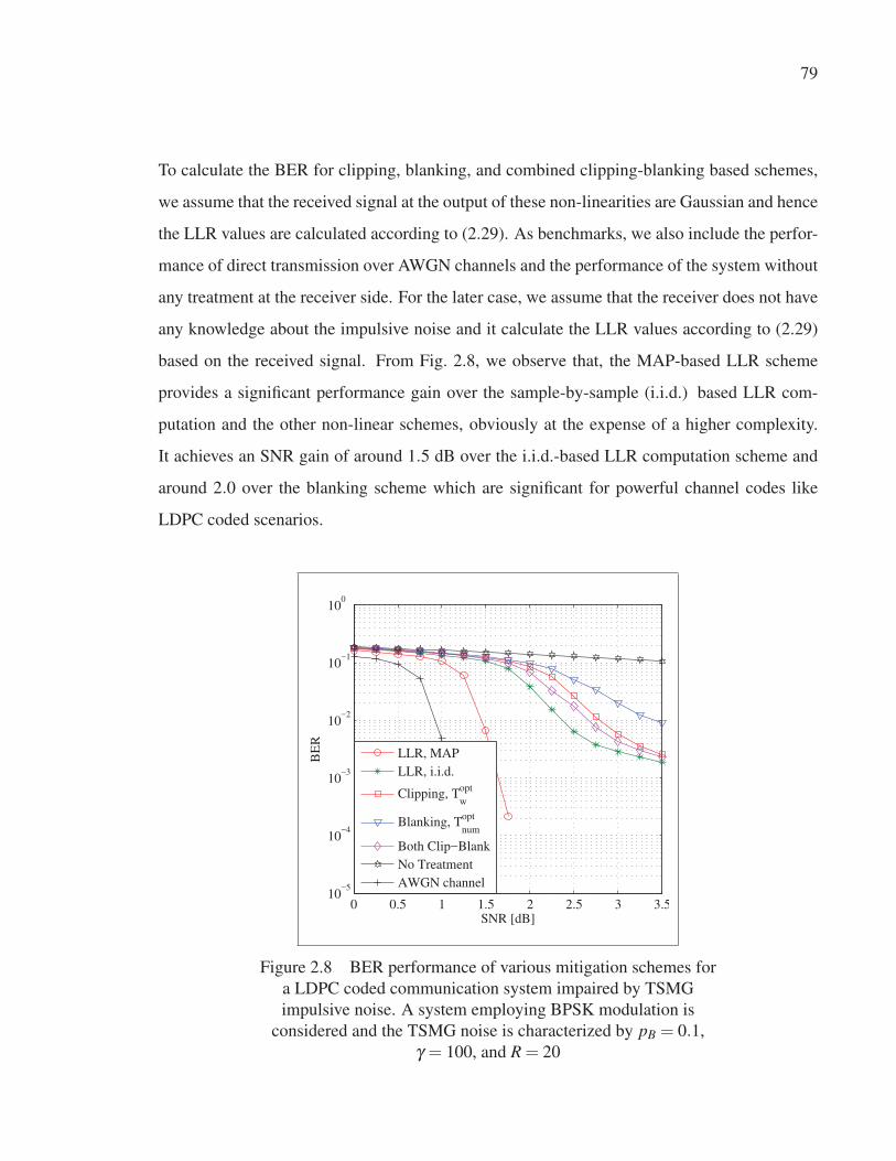
79

To calculate the BER for clipping, blanking, and combined clipping-blanking based schemes,

we assume that the received signal at the output of these non-linearities are Gaussian and hence

the LLR values are calculated according to (2.29). As benchmarks, we also include the perfor-

mance of direct transmission over AWGN channels and the performance of the system without

any treatment at the receiver side. For the later case, we assume that the receiver does not have

any knowledge about the impulsive noise and it calculate the LLR values according to (2.29)

based on the received signal. From Fig. 2.8, we observe that, the MAP-based LLR scheme

provides a significant performance gain over the sample-by-sample (i.i.d.) based LLR com-

putation and the other non-linear schemes, obviously at the expense of a higher complexity.

It achieves an SNR gain of around 1.5 dB over the i.i.d.-based LLR computation scheme and

around 2.0 over the blanking scheme which are significant for powerful channel codes like

LDPC coded scenarios.

0 0.5 1 1.5 2 2.5 3 3.510

−5

10−4

10−3

10−2

10−1

100

SNR [dB]

BE

R

LLR, MAPLLR, i.i.d.

Clipping, Twopt

Blanking, Tnumopt

Both Clip−BlankNo TreatmentAWGN channel

Figure 2.8 BER performance of various mitigation schemes for

a LDPC coded communication system impaired by TSMG

impulsive noise. A system employing BPSK modulation is

considered and the TSMG noise is characterized by pB = 0.1,

γ = 100, and R = 20

80

Fig. 2.9 also shows the performance improvement brought by the LLR computation in case

of when we consider γ = 1 in the TSMG noise process which corresponds to the Bernoulli-

Gaussian noise. Precisely, when the exact impulsive noise statistics is exploited in the LLR

computation, we achieve a significant performance gain irrespective of the noise process. Inter-

estingly, from Fig. 2.9, we also remark that while the LLR computation using MAP algorithm

shows better performance than the sample-by-sample LLR calculation for TSMG noise, the

later shows the same performance in case of Bernoulli-Gaussian noise. This confirms that, for

Bernoulli-Gaussian noise, the optimal LLR computation using MAP algorithm simplifies to

memoryless sample-by-sample algorithm. In addition, as in TSMG noise, the clipping scheme

shows better performance than the blanking scheme, whereas the combined clipping-blanking

scheme outperforms the clipping scheme in the higher SNR regions by taking the advantages

of both clipping and blanking schemes.

0 1 2 3 410

−7

10−6

10−5

10−4

10−3

10−2

10−1

100

SNR [dB]

BE

R

LLR, MAPLLR, i.i.d.

Clipping, Twopt

Blanking, Tnumopt

Both Clip−BlankNo TreatmentAWGN channel


a LDPC coded communication system impaired by

Bernoulli-Gaussian impulsive noise. A system employing BPSK

modulation is considered and the Bernoulli-Gaussian noise is

characterized by pB = 0.1 and R = 20

81

Furthermore, we also investigate the performance of the considered schemes when we set the

TSMG noise parameter R = 100 instead of R = 20. The resulting BER performance is shown

in Fig. 2.10. As portrayed in the figure, when the value of R increases, i.e, when the impulsive

noise component becomes more powerful compared to the Gaussian noise component, the per-

formance of the blanking scheme outperforms the clipping scheme and the performance of the

combined clipping-blanking scheme approaches the sample-by-sample LLR scheme. Hence,

it can be concluded that the choice of the most suitable non-linear preprocessing technique

depends on the application noise environment.

0 0.5 1 1.5 2 2.5 3 3.510

−4

10−3

10−2

10−1

100

SNR [dB]

BE

R

LLR, MAPLLR, i.i.d.

Clip, Twopt

Blank, Tnumopt

Both Clip−BlankNo Treatment


a LDPC coded communication system impaired by TSMG

impulsive noise. A system employing BPSK modulation is

considered and the TSMG noise is characterized by pB = 0.1,

γ = 100, and R = 100

82

2.6 Exact LLR Derivation when using a Non-linearity

Here, we consider the exact LLR calculation when the clipping and blanking operations are

realized. The LLR of the clipped or blanked signal rk is defined as

L(rk) = lnPR (rk|xk = 1)

PR (rk|xk =−1)(2.30)

where PR is the PDF of the non-linearity output rk. The conditional PDFs PR (rk|xk) after the

clipping and blanking operations are respectively given by Ndo, G. (2010)

P(c)R (rk|xk) = PY (rk|xk)+δ (rk +T )PY (yk <−T |xk)+δ (rk −T )PY (yk > T |xk) (2.31)

P(b)R (rk|xk) = PY (rk|xk)+δ (rk) [PY (yk <−T |xk)+PY (yk > T |xk)] (2.32)

where PY (rk|xk) can be obtained according to (2.25) and

PY (yk > T |xk) = pGQ(

T −1

σG

)+ pBQ

(T −1

σB

)(2.33)

PY (yk <−T |xk) = pGQ(

T +1

σG

)+ pBQ

(T +1

σB

)(2.34)

where Q(x) denotes the Q-function and δ (x) is the Kronecker symbol given by

δ (x) =

⎧⎨⎩ 1 if x = 0

0 if x = 0(2.35)

On the other hand, for the blanking scheme, the LLR before and after the non-linearity is the

same, i.e,

L(b)(rk) = L(yk). (2.36)

Fig. 2.11 shows the BER performances obtained for a LDPC coded BPSK modulated trans-

mission over TSMG noise where the clipping operation is performed and the exact LLR is

computed at the output of the clipped signal. From Fig. 2.11, we observe that the performance

of the considered scheme improves with the increase of the clipping threshold T and con-

83

verges to the LLR performance obtained without clipping. This result confirms that the exact

LLR computation after the clipping, blanking non-linearity does not provide any improvement

compared to the case when the exact LLR of the received signal is computed without any

pre-treatment.

0 0.5 1 1.5 2 2.5 3 3.510

−5

10−4

10−3

10−2

10−1

100

SNR [dB]

BE

R

LLRClip+LLR, T=2Clip+LLR, T=2.5Clip+LLR, T=3Clip+LLR, T=4

Figure 2.11 BER variations of the combined clipping and LLR

operations over TSMG noise. In the simulations it is assumed that

pB = 0.1, γ = 100, and R = 20

2.7 Conclusion

In this paper, we evaluated some practical impulsive noise mitigation techniques for LDPC

coded single-carrier systems subject to bursty impulsive noise modelled by a Markov-Gaussian

process. The provided simulation results showed that the LLR-based impulsive noise miti-

gation technique with the MAP detection criterion outperforms the simple but more popular

clipping, blanking, and combined clipping/blanking schemes at the expense of higher compu-

84

tational complexity. This is caused by the imperfect level of clipping and blanking of signal

samples affected by impulsive noise due to the lack of noise memory information in the mitiga-

tion process. It is also shown that there always exists an optimal clipping, blanking threshold

that minimizes the BER and that this optimal threshold value changes with the SNR varia-

tions. In this paper, an optimal threshold determination based on good detection and false

alarm trade-off has been investigated considering two optimization criterion namely: weighted

combination criterion and seigert criterion. We further showed that the optimal LLR computa-

tion with clipping, blanking pretreatment does not provide any improvement in the mitigation

performance. This finding proves that the LLR-based mitigation scheme can be considered as

the most promising method for the mitigation of the harmful effects of bursty impulsive noise.

In this paper, we have only discussed the mitigation techniques for TSMG noise where the

number of states are restricted to two. The mitigation techniques for Markov Middleton noise

will be investigated in our future research.

CHAPTER 3

PERFORMANCE ANALYSIS OF DF COOPERATIVE RELAYING OVER BURSTYIMPULSIVE NOISE CHANNEL

Md Sahabul Alam 1, Fabice Labeau 2, Georges Kaddoum1


1100 Notre-Dame Ouest, Montréal, Québec, Canada H3C 1K32 Department of Electrical Engineering, McGill University,

845 Sherbrooke St. Ouest, Montréal, Québec, Canada H3A 0G4

Article published in IEEE Transactions on Communications, July, 2016.

3.1 Abstract

In this article, we consider the performance analysis of a decode-and-forward (DF) cooperative

relaying (CR) scheme over channels impaired by bursty impulsive noise. Although, Middleton

class-A model and Bernoulli-Gaussian model give good results to generate a sample distri-

bution of impulsive noise, they fail in replicating the bursty behavior of impulsive noise, as

encountered for instance within power substations. To deal with that, we adopt a two-state

Markov-Gaussian process for the noise distribution. For this channel, we evaluate the bit error

rate (BER) performance of direct transmission (DT) and a DF relaying scheme using M-ary

phase shift keying (M-PSK) modulation in the presence of Rayleigh fading with a maximum

a posteriori (MAP) receiver. From the obtained results, it is seen that the DF CR scheme in

bursty impulsive noise channel still achieves the space diversity and performs significantly bet-

ter than DT under the same power consumption. Moreover, the proposed MAP receiver attains

the lower bound derived for DF CR scheme, and leads to large performance gains compared

to the conventional receiving criteria which were optimized for additive white Gaussian noise

(AWGN) channel and memoryless impulsive noise channel.

86

3.2 Introduction

The noise characteristics in many environments, such as around power transmission lines,

power substations, and in some mobile radio scenarios are highly non-Gaussian and are in-

herently impulsive in nature Middleton (1977). For example, in power substations the noise

emitted from power equipments, such as transformers, busbars, circuit-breakers, and switch-

gears are impulsive Hikita et al. (1998); Portuguds et al. (2003); Sacuto et al. (2012). For

smart grid technology Hossain, E., Han, Z. & Poor, H. V. (2012), in order to assist the elec-

tricity transportation via control, interaction with, and monitoring of power equipment from

outside the station, a communication network must be operational within the substation. This

could be accomplished by deploying a wireless sensor network (WSN) Gungor et al. (2010);

Tuna et al. (2013) where the deployed sensor nodes collect information from the pieces of

equipment, and send their sensed information to the remote smart grid monitoring center for

further process. In such applications, the generated impulsive noise from the substation equip-

ment that affects the wireless links between the sensor nodes displays a bursty behaviour as

observed in experimental measurements Sacuto et al. (2012). The models commonly used in

the literature to represent impulsive noise are either Middleton class-A Middleton (1977) or

Bernoulli-Gaussian Ghosh (1996). Although these models give good results to generate a sam-

ple distribution of impulsive noise, they cannot describe the bursty nature of the impulses, i.e.,

the correlation among the noise samples in the time domain. To handle this, Markov chain

models have been investigated in the literature Fertonani & Colavolpe (2009); Mitra & Lampe

(2010); Mushkin & Bar-David (1989); Ndo et al. (2013), representing the impulsive noise

characteristics by including a significant amount of memory.

One of the designing challenges for WSN-based smart grid monitoring applications is how

reliably the sensor nodes send their sensed data to the substation monitoring center Gungor

et al. (2010); Tuna et al. (2013). Cooperative WSNs where the sensor nodes cooperate among

each other can be one of the promising candidates for transmission in impulsive channels due

to its reliability over fading and interference channels Laneman et al. (2004); Nosratinia et al.

(2004). It is based on the broadcast nature of the wireless medium and achieves the potentials

87

of spatial diversity in wireless networks without necessitating the placement of multiple anten-

nas at each node. It is very attractive for WSN since the sensor nodes cannot afford multiple

antennas due to their size and cost constraints. The two most popular relaying strategies are

DF relaying and amplify-and-forward (AF) relaying. Although there exists a large number of

publications on these relaying schemes in various aspects, many of them are restricted to the

AWGN assumption. In practice, AWGN is a common assumption to bundle together a lot of

sources of noise, beyond thermal. The performance of CR in impulsive channel has only been

considered in the literature recently. The pairwise error probability (PEP) of AF CR scheme

over flat fading channel in the presence of impulsive noise modeled by Middleton class-A

has been investigated in Al-Dharrab & Uysal (2009a); Al-Dharrab, S. & Uysal, M. (2009b).

Upper bounds on PEP expressions are derived for both space time block coded scheme and

repetition-based coded scheme. Simulation results demonstrated that the performance of co-

operative systems highly depends on the impulsive nature of the noise and different diversity

orders are achieved in different signal-to-noise ratio (SNR) regions. Similar performance anal-

ysis is carried out in Savoia & Verde (2011) for DF CR schemes. It is shown that similar to

the Gaussian noise case, the system achieves full diversity order asymptotically with SNR in

impulsive noise scenario. The authors in Siamack, G., Jamil, H., Tarlochan, S. S. & Serguei,

P. (2012) studied the impact of impulsive noise modeled by a Bernoulli-Gaussian process on

the performance of cooperative relaying system in a smart grid scenario. It is shown that as

the impulse occurs, probability increases, the performance of the system is getting worse. In

Nasri & Schober (2010), closed-form asymptotic symbol-error rate (SER) and BER expres-

sions were derived for an AF CR scheme with multiple relays which is valid for arbitrary

non-Gaussian noise and interference with finite moments. The simulation results reveal that,

at high SNR, full diversity order is obtained and is independent of the type of noise. While

the above papers quantify the diversity advantages in the presence of impulsive noise, the au-

thors in Van Khuong & Le-Ngoc (2010,1) studied the performance of DT and DF CR schemes

over flat Rayleigh fading and Bernoulli-Gaussian impulsive noise assuming different receiving

structures at the destination. The obtained results showed that DF CR performs significantly

better than DT under the same bandwidth efficiency and power consumption. It is also shown

88

that while the optimal Bayes receiver Tepedelenlioglu & Gao (2005) and the maximum ratio

combining (MRC) have the same diversity order as expected, the optimal Bayes receiver ob-

tains an additional 3dB SNR gain over the MRC combiner by considering impulsive noise in

the detection process. The above results motivate us to consider the performance analysis of

CR over correlated impulsive noise channel. While the complexity of DF relaying is higher

than AF relaying duo to its digital processing, we consider DF relaying in our analysis since it

reduces the effects of additive noise at the relay Fareed, M. M. & Uysal, M. (2009).

However, all of the above performance analyses for CR schemes have been carried out over

independent and identically distributed (i.i.d.) impulsive channels1, which cannot include

any information on noise time-correlation. To address this issue, we consider a two-state

Markov-Gaussian process Fertonani & Colavolpe (2009) for noise modeling. A two-state

Markov-Gaussian process is a simple and effective way to model a bursty impulsive noise

channel Fertonani & Colavolpe (2009); Mitra & Lampe (2010). In this context, the authors

in Mushkin & Bar-David (1989) calculate the capacity of a Gilbert-Elliott channel which is a

varying binary symmetric channel with memory. It is shown that the capacity of the channel

increases monotonically with increasing the utilization of memory information at the receiver

side and converges to a maximum value which is the capacity of the same channel when per-

fect state information is available at the receiver. It is also shown that, even if the memory of

the channel is ignored through proper interleaving, the capacity of the interleaved channel is

lower than the capacity of the original channel. The authors in Fertonani & Colavolpe (2009)

compute the achievable information rate of a two-state Markov-Gaussian channel through an

information-theoretic analysis. We would like to point out that, while the state process of a

two-state Markov-Gaussian noise model is the same as in a Gilbert-Elliott model, the same

analytical arguments do not lead to a closed-form expression for this model since the channel

output alphabet is non-binary Fertonani & Colavolpe (2009); Mitra & Lampe (2010). Hence,

Fertonani & Colavolpe (2009) evaluates the information rate of this channel by means of the

simulation-based method described in Arnold, D. M., Loeliger, H.-A., Vontobel, P. O., Kavcic,

1 Throughout the article, the terms ‘impulsive noise’ and ‘impulsive channel’ are used interchangeably.

89

A. & Zeng, W. (2006). It is shown that the ultimate performance limit of such channels im-

proves as the channel memory becomes more significant. Aims at approaching the ultimate

performance limit as close as possible, Fertonani & Colavolpe (2009) provides a transceiver

architecture for DT-based on powerful codes and iterative detection. It is shown that the pro-

posed MAP-based iterative receiver with LDPC channel coding is able to exploit the memory

of the noise process at the receiver and perform fairly close to the ultimate limit. To the best

of our knowledge, no research results have been published on CR schemes impaired by such

bursty impulsive channels. Here, we provide a mathematical framework for the performance

analysis of DF CR schemes over bursty impulsive noise channel. Our work is an extension

of Fertonani & Colavolpe (2009) to the CR scenario. While we do not attempt to modify the

MAP detector proposed in Fertonani & Colavolpe (2009) to exploit the channel memory, our

analysis also includes uncoded scenario and derive analytical error rate expressions for the

proposed system, thus providing a framework to validate the simulation results. We expect

to gain more compared to the optimal memoryless receiver Tepedelenlioglu & Gao (2005);

Van Khuong & Le-Ngoc (2010) proposed for CR scheme over impulsive noise channel by

considering noise memory in the detection process. Two different relaying strategies are con-

sidered depending on the processing performed by the relay: simple DF relaying (SR) and

selective DF relaying (SDFR). In simple DF relaying, the relay transmits all the symbols it

receives, whereas, in selective DF relaying, it is assumed that the relay forwards its decoded

signal only if the received SNR at the relay is greater than a certain threshold, otherwise the re-

lay remains silent and the destination decodes based on the direct transmission from the source

only.

The contributions of this work are as follows. First, we derive a SER formula for DT using

M-PSK modulation in the presence of Rayleigh frequency flat fading and two-state Markov-

Gaussian impulsive noise. To validate the derived SER formula for DT, we considered the

optimal MAP detection criterion that has been used in Fertonani & Colavolpe (2009) for sym-

bol detection in a two-state Markov-Gaussian noise, and adapt the Bahl-Cocke-Jelinek-Raviv

(BCJR) algorithm Bahl et al. (1974) to be implemented in the detector for this case. Then, we

90

extend the derived SER formula for DT to the case of DF CR schemes and provide a lower

bound under the hypothetical assumption that the receivers have the knowledge of the state of

the noise process. Finally, we propose an optimal MAP receiver for the considered DF CR

schemes that utilize the MAP detection criterion for each link.

It is shown that the proposed optimal MAP receiver achieves the lower bound derived for

DF CR scheme and performs significantly better than the conventional schemes developed for

AWGN channel and memoryless impulsive noise channel. Indeed, the BER obtained with the

memoryless receiver can be divided by almost 103 to get the BER with optimal MAP receiver

under coded transmission. Also, DF CR schemes perform significantly better than DT under

the same power consumption. In addition, for simple relaying, using the BER of the relay at

the destination, the proposed optimal MAP receiver performs significantly better than the case

where the MAP receiver does not have any knowledge about the error at the relay and achieves

similar performance as that obtained through selective DF relaying.

The rest of the paper is organized as follows. In Section 3.3, the system model is introduced

and Section 3.4 provides an overview of two-state Markov-Gaussian process. In Section 3.5,

we provide the mathematical framework for the proposed scenario. Section 3.6 provides the

performances in terms of BER and finally, some conclusions are drawn in Section 3.7.

3.3 System model

Here, we consider a DF cooperative relaying scheme with single relay (m), as shown in Fig 3.1,

where the data transmission between the source-destination (sd) pair is assisted by m. We as-

sume that all nodes are equipped with a single antenna and share the same bandwidth for data

transmission. We also assume that each node operates in half-duplex mode and hence cannot

transmit and receive simultaneously. Both s and m terminals use time division multiplexing for

channel access. The cooperative communication takes place in two time slots, with normalized

time intervals t0 and t1 = 1− t0. In the first time slot, s transmits the data to d, and due to the

broadcast nature of the wireless channel, m also receives it. The relay then demodulates and

91

s

m

d

m

s d

First time slot Second time slot

λsm

λsd

λmd

Figure 3.1 Cooperative communication with half-duplex

relaying

decodes the received signal to recover the source information and based on the relaying strat-

egy, it either retransmits in the second time slot of duration t1, or declares that it will remain

silent. During this period, s remains in the silent mode as indicated by the dotted line in Fig 3.1.

For simple DF relaying, the relay always retransmits the decoded data to the destination in the

second time slot. The destination then receives the noisy observation sequences from s in the

first time slot as well as from m in the second time slot. The overall operation is shown in

Fig 3.1. Hence, the decoded data with possible errors are forwarded from the relay to the des-

tination. It is different from most papers on single-relay DF CR schemes where it is typically

assumed that if the relay decodes the source message perfectly it will forward its decoded in-

formation to the destination, otherwise it will stay in silent mode, i.e., what we call selective

DF relaying Laneman et al. (2004), which is decided by comparing the received SNR at the

relay to a given threshold. However, in practical relaying systems an arbitrary chosen threshold

does not guarantee error-free detection and hence decoding errors may occur at the relay Lee,

K. & Hanzo, L. (2009); Liang, D., Ng, S. X. & Hanzo, L. (2010); Sneessens, H. H., Louveaux,

J. & Vandendorpe, L. (2008) even if the received SNR at the relay is greater than a predeter-

mined threshold value. Therefore, though the destination assumes that perfect decoded data

were transmitted from the relay, actually the forwarded data may contain hard decision errors.

So, there will be a performance degradation if the relay can not be guaranteed to be error-free.

Specially, this problem becomes more crucial when the relay moves away from the source

92

and becomes closer to the destination. Although this problem could be solved by considering

cyclic redundancy check (CRC) checking at the relays, it is bandwidth-consuming Wang, T.,

Cano, A., Giannakis, G. B. & Laneman, J. N. (2007) and induces extensive overhead since

CRC checking usually takes place at the MAC layer. The authors in Jayakody, D. N. & Flana-

gan, M. F. (2015); Jayakody, D. N., Li, J. & Flanagan, M. F. (2015) and the references therein

consider soft information relaying to mitigate the effect of decoding error propagation from the

relay to the destination. It is shown that soft relaying performs better than hard information

relaying under poor source-relay link conditions. However, these schemes require complex

offline computation of soft noise parameters which increases the complexity of decoding at the

destination for real-time transmission. To avoid these, our analysis remains more general and

considers that decoding error might be propagated by the relay.

Consider that the source s generates a frame of binary information of length L bits (b0, . . . ,bL−1),

mapped into a M-PSK modulated sequence (xs,0,xs,1, . . . ,xs,K−1), and transmitted to both m and

d in the first time slot. The signals received at m and d at each time epoch k, k = 0,1, . . . ,K−1

can be respectively expressed as

ysm,k =√

Pshsm,kxs,k +nsm,k, (3.1)

ysd,k =√

Pshsd,kxs,k +nsd,k, (3.2)

where Ps is the average source transmission power for each symbol, xs,k is the transmitted sym-

bol from s, hi j,k is the channel coefficient for the i j link, i∈ (s,m) and j ∈ (m,d), and ni j,k is the

noise term for the i j link that captures the combined effects of AWGN and the impulsive inter-

ferers. We assume independent Rayleigh fading in all links, i.e., for each i j link, hi j ≡ ai je jθi j

is modeled as a zero-mean, independent, circularly symmetric complex Gaussian random vari-

able with variance Ωi j ≡ ε{|hi j|2} = 1/λ ηi j , where ε{·} denotes expectation operator, λi j is

the relative distance of i from j, and η is the path loss exponent. Hence, the channel ampli-

tudes, ai j are Rayleigh distributed, whereas the channel phases, θi j are uniformly distributed

in [−π,π). It is assumed that the channel coefficients are known by the receiver side, but not

93

by the transmitter side. The noise sample ni j,k is modeled as a two-state Markov-Gaussian

process, which is in fact a Markov process in with the marginal distribution in each state are

Gaussian. In the following section we will provide an overview of the model and explain the

physical significance of each parameter. We assume that the noise samples for each link are

mutually independent of the other links.

In the second time slot, at m, the received signal ysm is passed through a demodulator to recover

the source information. The relay then decodes the source information, potentially making an

error. After recovering the source information, the relay modulates it using the same modula-

tion format as in s and forwards it to the destination with average transmission power Pm. The

signal received at the destination in this case is given by

ymd,k =√

Pmhmd,kxm,k +nmd,k, (3.3)

where xm,k is the transmitted signal from m. For fair comparison between DT and CR schemes,

in our discussion we assume that the total source transmission power for direct transmission

PT is equal to the sum of source and relay transmission power in cooperative communication

and hence the total transmission power is constrained as follows:

Ps +Pm = PT . (3.4)

3.4 An overview of two-state Markov-Gaussian model

A two-state Markov-Gaussian model is introduced by Fertonani Fertonani & Colavolpe (2009)

to characterize the correlated impulsive noise. At each time epoch k, the statistical properties

of the noise sample ni j,k are completely defined by the channel state sk ∈ {G,B}. In our noise

modeling, G stands for the good channel that is impaired by the background Gaussian noise

only and B for the bad channel which is impaired by impulsive interferers also. For each i j

link, we model ni j,k as a zero-mean, circularly symmetric complex Gaussian random variable

with variances depending on sk, so that conditioned on sk, the probability density functions

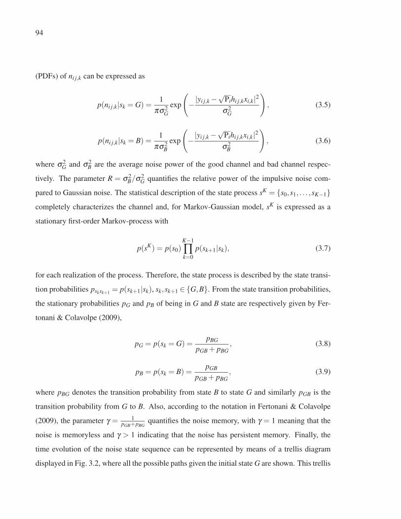
94

(PDFs) of ni j,k can be expressed as

p(ni j,k|sk = G) =1

πσ2G

exp

(−|yi j,k −

√Pihi j,kxi,k|2

σ2G

), (3.5)

p(ni j,k|sk = B) =1

πσ2B

exp

(−|yi j,k −

√Pihi j,kxi,k|2σ2

B

), (3.6)

where σ2G and σ2

B are the average noise power of the good channel and bad channel respec-

tively. The parameter R = σ2B/σ2

G quantifies the relative power of the impulsive noise com-

pared to Gaussian noise. The statistical description of the state process sK = {s0,s1, . . . ,sK−1}completely characterizes the channel and, for Markov-Gaussian model, sK is expressed as a

stationary first-order Markov-process with

p(sK) = p(s0)K−1

∏k=0

p(sk+1|sk), (3.7)

for each realization of the process. Therefore, the state process is described by the state transi-

tion probabilities psksk+1= p(sk+1|sk), sk,sk+1 ∈ {G,B}. From the state transition probabilities,

the stationary probabilities pG and pB of being in G and B state are respectively given by Fer-

tonani & Colavolpe (2009),

pG = p(sk = G) =pBG

pGB + pBG, (3.8)

pB = p(sk = B) =pGB

pGB + pBG, (3.9)

where pBG denotes the transition probability from state B to state G and similarly pGB is the

transition probability from G to B. Also, according to the notation in Fertonani & Colavolpe

(2009), the parameter γ = 1pGB+pBG

quantifies the noise memory, with γ = 1 meaning that the

noise is memoryless and γ > 1 indicating that the noise has persistent memory. Finally, the

time evolution of the noise state sequence can be represented by means of a trellis diagram

displayed in Fig. 3.2, where all the possible paths given the initial state G are shown. This trellis

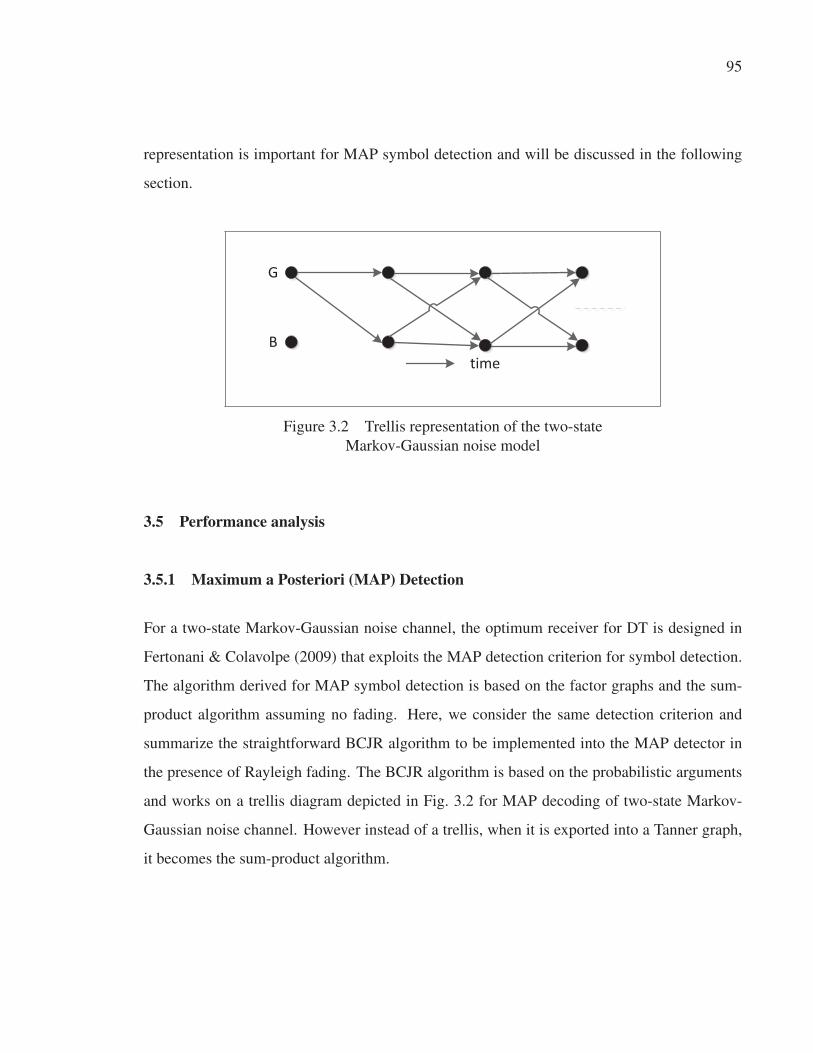
95

representation is important for MAP symbol detection and will be discussed in the following

section.

G

Btime



3.5 Performance analysis

3.5.1 Maximum a Posteriori (MAP) Detection

For a two-state Markov-Gaussian noise channel, the optimum receiver for DT is designed in

Fertonani & Colavolpe (2009) that exploits the MAP detection criterion for symbol detection.

The algorithm derived for MAP symbol detection is based on the factor graphs and the sum-

product algorithm assuming no fading. Here, we consider the same detection criterion and

summarize the straightforward BCJR algorithm to be implemented into the MAP detector in

the presence of Rayleigh fading. The BCJR algorithm is based on the probabilistic arguments

and works on a trellis diagram depicted in Fig. 3.2 for MAP decoding of two-state Markov-

Gaussian noise channel. However instead of a trellis, when it is exported into a Tanner graph,

it becomes the sum-product algorithm.

96

For M-PSK modulation scheme with M = 2, the MAP decoding rule at the destination is given

by

xs,k =

⎧⎨⎩ 1 if Lk ≥ 0

−1 if Lk < 0(3.10)

where, xs,k is the estimate of the source’s transmitted sequence xs,k generated at d and Lk is the

log-likelihood ratio (LLR). For direct transmission, Lk at the destination is defined by

Lsd,k = ln

{p(xs,k = 1|yK

sd)

p(xs,k =−1|yKsd)

}, (3.11)

where yKsd = {ysd,0,ysd,1, . . . ,ysd,K−1} is the whole sequence to be detected and K is the size of

the sequence. For computation, at each k, the optimal MAP detector at the destination evaluates

the a posteriori probability p(xs,k|yKsd) for each symbol xs,k belonging to the binary modulation

alphabet {1,-1}. The a posteriori probability p(xs,k = b | yKsd), b ∈ {1,−1} can be computed

from

p(xs,k = b|yKsd) ∝ p(xs,k = b,yK

sd) = ∑sk,sk+1

p(xs,k = b,yKsd,sk,sk+1) (3.12)

where sk,sk+1 denote the noise states at time k and k+ 1 respectively and the proportionality

indicates that the two sides may differ with a positive multiplicative factor that does not have

any effect on the detection process Fertonani & Colavolpe (2009). Let us define the following

quantities

αk(sk) = p(ysd,0,ysd,1, . . . ,ysd,k−1,sk), (3.13)

βk(sk) = p(ysd,k,ysd,k+1, . . . ,ysd,K−1|sk), (3.14)

δk(xs,k,sk,sk+1) = p(sk+1|sk)p(nsd,k = ysd,k −√

Pshsd,kxs,k|sk) (3.15)

where αk(sk) and βk(sk) are referred to as the forward and backward filters and δk(xs,k,sk,sk+1)

represents the branch metrics of the trellis diagram shown in Fig. 3.2. For a two-state Markov-

Gaussian model, the quantity p(nsd,k = ysd,k −√

Pshsd,kxs,k|sk) is given by (3.5) and (3.6) re-

spectively. Assuming independent transmitted symbols xs,k, using (3.13), (3.14), and (3.15),

97

the probability term p(xs,k = b,yKsd,sk,sk+1) in (3.12) can be represented as

p(xs,k = b,yKsd,sk,sk+1) = p(xs,k = b)αk(sk)βk+1(sk+1)δk(xs,k = b,sk,sk+1), (3.16)

Thus, from (3.12)

p(xs,k = b,yKsd) = p(xs,k = b) ∑

sk,sk+1

αk(sk)βk+1(sk+1)δk(xs,k = b,sk,sk+1), (3.17)

Then, the LLR values at the destination are obtained by

Lsd,k = ln

{p(xs,k = 1,yK

sd)

p(xs,k =−1,yKsd)

}

= ln

{p(xs,k = 1)∑sk,sk+1

αk(sk)βk+1(sk+1)δk(xs,k=1,sk,sk+1)

p(xs,k =−1)∑sk,sk+1αk(sk)βk+1(sk+1)δk(xs,k=−1,sk,sk+1)

}. (3.18)

The forward and backward filters can be computed recursively as

αk+1(sk+1) = ∑sk,xs,k

αk(sk)p(xs,k)δk(xs,k,sk,sk+1), (3.19)

βk(sk) = ∑sk+1,xs,k

βk+1(sk+1)p(xs,k)δk(xs,k,sk,sk+1), (3.20)


α0(s0 = S) = pS, and βK(sK = S) = 1. S ∈ (G,B) (3.21)

However, for M-PSK modulation scheme with M > 2, the first step is to compute the a poste-

riori probability p(xi,k|yi j,k) for each symbol xi,k belonging to the M-PSK modulation alphabet

using the MAP symbol detector explained above. The next step is to consider a standard soft

demapper Tosato, F. & Bisaglia, P. (2002) which performs reliable metric computation at the

bit level, given the input probability p(xi,k|yi j,k). Note that, this block is not needed in case

of BPSK since the generated LLR values for the BPSK symbols are the same as the bits. The

98

demapper extracts the quantity p(bl,k = b|yi j,k) through the input-output relationship given by

p(bl,k = b|yi j,k) ∝ ∑xi,k∈χ(l,b)

p(xi,k|yi j,k), (3.22)

where bl,k is the lth bit of symbol xi,k and χ(l,b) denote the set of xi,k symbols having their lth

bit equal to b. For example, the LLR values for the first and second bit in Q-PSK modulation

scheme can be obtained by

L(1)i j,k = ln

{b1,k = 0|yi j,k

b1,k = 1|yi j,k

}= ln

{(xi,k = 00|yi j,k)+(xi,k = 01|yi j,k)

(xi,k = 10|yi j,k)+(xi,k = 11|yi j,k)

}. (3.23)

L(2)i j,k = ln

{b2,k = 0|yi j,k

b2,k = 1|yi j,k

}= ln

{(xi,k = 00|yi j,k)+(xi,k = 10|yi j,k)

(xi,k = 01|yi j,k)+(xi,k = 11|yi j,k)

}. (3.24)

It should be mentioned that in order to evaluate the LLR values required for the evaluation of

the BER, the receivers need the knowledge of the noise parameters (pB,γ,R,σ2G) and the am-

plitude of the channel coefficients hi j. Similar to Fertonani & Colavolpe (2009), it is assumed

that these parameters are perfectly known at the receiver side. This assumption is made since

we are mainly interested to focus on the BER performance comparison of different receivers,

and to evaluate the impact of noise memory. How the receiver side gets these knowledge is

beyond the scope of this paper.

3.5.2 BER of Direct Transmission

In order to derive the analytical SER formula for direct transmission, we assume that the

destination receiver has the knowledge of the variance of each state. Then, for the consid-

ered two-state Markov-Gaussian noise, the conditional probability of symbol error for M-PSK

modulated signal when the channel is in good state is given by the integral expression(Simon,

M. K. & Alouini, M.-S., 2005, Eq. (8.23))

PGe,DT =

1

π

∫ (M−1)π/M

0exp

(−PT

σ2G

gPSK

sin2 θ

), (3.25)

99

where gPSK = sin2(π/M). Similarly, the conditional SER when the channel is in bad state is

given by

PBe,DT =

1

π

∫ (M−1)π/M

0exp

(−PT

σ2B

gPSK

sin2 θ

), (3.26)

Assuming that the receiver has knowledge of the state sk, a lower bound on the average SER

for the direct transmission is expressed as

Pe,DT = psdG PG

e,DT + psdB PB

e,DT , (3.27)

where psdG = psd

BG/psdGB + psd

BG and psdB = psd

GB/psdGB + psd

BG are the steady-state probabilities of

having in good state and bad state respectively for the sd link. When fading is present, the

conditional SER for a given channel realization hsd is expressed as

Pe,DT (hsd) =psd

Gπ

∫ (M−1)π/M

0exp

(−γsd

GgPSK

sin2 θ

)+

psdBπ

∫ (M−1)π/M

0exp

(−γsd

BgPSK

sin2 θ

),

(3.28)

where, γsdG = PT|hsd |2

σ2G

and γsdB = PT|hsd |2

σ2B

are the instantaneous link SNRs for the sd link in good

and bad state respectively. Since hsd ∼ CN(0,Ωsd), i.e., the link experience Rayleigh fading,

γsdu is exponentially distributed with the probability density function

fγsdu(γ) =

1

γsdu

e− γ

γsdu , (3.29)

where, γsdu = ε{γsd

u }= PTΩsdσ2

u,sdincorporates the average SNR of sd link, u ∈ (0,1)≡ (G,B) and

σ2u,sd = Ru

sdσ2G is the variance of nsd with Rsd is the impulsive to Gaussian noise power ratio

for the sd link. By averaging (3.28) with respect to the random variable γsdu and making use of

(Simon & Alouini, 2005, Eq. (8.113)), the average SER is given by

Pe,DT =1

∑u=0

(M−1

M

){1−

√gPSK γsd

u

1+gPSK γsdu

(M

(M−1)π

)[π2+tan−1

(√gPSK γsd

u

1+gPSK γsdu

cotπM

)]}.

(3.30)

100

For BPSK (M = 2), (3.30) becomes the BER of direct transmission

Pb,DT =psd

G2

(1−

√γsd

G

1+ γsdG

)+

psdB2

(1−

√γsd

B

1+ γsdB

). (3.31)

3.5.3 BER of DF Cooperative Relaying

In case of DF cooperative relaying, the SER at the relay follows the same form as in (3.30),

i.e.,

Pe,m =1

∑u=0

(M−1

M

){1−

√gPSK γsm

u1+gPSK γsm

u

(M

(M−1)π

)[π2+tan−1

(√gPSK γsm

u1+gPSK γsm

ucot

πM

)]}.

(3.32)

where, γsmu = PTΩsm

Rusmσ2

G, u ∈ {G,B} is the average received SNR of sm link. The end-to-end SER

performance of DF cooperative relaying scheme depends on different relaying strategies such

as SR in which the relay always transmits in the second phase. The end-to-end SER under this

condition is equal to

PSRe,coop = Pe,m ·Per

e,smd +(1−Pe,m) ·Pnere,smd, (3.33)

where Pere,smd is the probability of error at the destination after combining the two signals coming

from the source and the relay when the error is propagated from the relay. Also, Pnere,smd is the

probability of error at the destination when there is no error propagation from the relay and

hence the source and the relay will transmit the same data. On the other hand, in SDFR it is

assumed that the relay forwards its decoded signal only if the source-relay SNR is larger than

a certain threshold, otherwise the relay remains silent and the destination decodes based on

the direct transmission from the source only. A lower bound of this protocol is obtained if it is

assumed that the relay is able to decode the source symbol successfully when the received SNR

at the relay is greater than a certain threshold and retransmits on the second phase only if it is

successfully decoded. The average SER at the destination under this scheme can be computed

as

PSDFRe,coop = Pe,m ·Pe,DT +(1−Pe,m) ·Pner

e,smd, (3.34)

101

However, in practical relaying systems, an arbitrary chosen threshold does not guarantee error-

free detection, and hence decoding errors may occur at the relay even if the received SNR at the

relay is greater than a predetermined threshold value. The actual average SER at the destination

for this scheme for a given threshold γt can be expressed as

PSDFRe,coop= p{γsm

u >γt}[Pe,m|γsm

u >γt ·Pere,smd+(1−Pe,m|γsm

u > γt) ·Pnere,smd

]+ p{γsm

u ≤γt} ·Pe,DT ,

(3.35)

Since γsmu is an exponential random variable with mean γsm

u , we have

p{γsmu ≤ γt}= 1− exp(−γt/γsm

u ) , (3.36)

When γsmu > γt , the SER at the relay decreases, but it remains nonzero regardless of the value

of γt Onat, F. A., Adinoyi, A., Fan, Y., Yanikomeroglu, H., Thompson, J. S. & Marsland, I. D.

(2008). Following the same procedure in Onat et al. (2008), for BPSK/Q-PSK modulation

scheme the BER at the relay given that γsmu > γt is equal to

Pb,m|γsmu >γt =

1

2

1

∑u=0

(psmB )u(psm

G )1−u

[er f c(

√γt)− eγt/γsm

u

√γsm

u1+ γsm

uer f c

(√γt

(1+

1

γsmu

))].

(3.37)

In order to compute Pere,smd and Pner

e,smd we have to know which combiner is used for combining

the signals coming from the source and the relay. For AWGN channel, i.e., when impulsive

noise is absent, the maximum ratio combining is optimal in the sense of minimizing the SER.

The MRC combining is

yd =√

Psh∗sdysd +√

Pmh∗mdymd. (3.38)

When impulsive noise is present, the optimal MAP combining is

Lcoop,k = ln

{p(xs,k = x0|yK

sd,yKmd)

p(xs,k = xz|yKsd,y

Kmd)

}

= ln

⎧⎪⎨⎪⎩

∑xm,k∈{x0,...,xz,...,xM−1}

p(xs,k = x0,xm,k|yKsd,y

Kmd)

∑xm,k∈{x0,...,xz,...,xM−1}

p(xs,k = xz,xm,k|yKsd,y

Kmd)

⎫⎪⎬⎪⎭ , (3.39)

102

where Lcoop,k is the symbol LLR value at the destination in case of cooperative communication.

Without loss of generality, it is assumed that the source transmits x0. Using the Bayes rule, the

following probability term is given by

p(xs,k,xm,k|yKsd,y

Kmd) =

p(yKsd,y

Kmd|xs,k,xm,k)p(xs,k,xm,k)

p(yKsd,y

Kmd)

, (3.40)

We assume that for the given transmitted signals, yKsd and yK

md are independent from each other.

Under this consideration, we have

p(yKsd,y

Kmd|xs,k,xm,k) = p(yK

sd|xs,k) · p(yKmd|xm,k), (3.41)

where the equality is due to the conditional independence of yKsd and yK

md and using the facts that

p(yKsd|xs,k,xm,k) = p(yK

sd|xs,k) and p(yKmd|xs,k,xm,k) = p(yK

md|xm,k). Substituting (3.41) in (3.39),

results in

Lcoop,k = ln

{p(xs,k = x0,yK

sd)

p(xs,k = xz,yKsd)

}+ ln

{p(xm,k=x0,yK

md)

p(xm,k = xz,yKmd)

}+ ln

⎧⎪⎨⎪⎩

1+ qm1−qm

(p(xm,k=xz,yK

md)

p(xm,k=x0,yKmd)

)

1+ qm1−qm

(p(xm,k=x0,yK

md)

p(xm,k=xz,yKmd)

)

⎫⎪⎬⎪⎭ .

(3.42)

where qm =∑M−1z=1 p(xm,k = xz|xs,k = x0) is the SER at the relay. With M-PSK modulation, there

are M−1 ways of making an incorrect decision at the relay and their impacts on the detection

process at the destination should be different. For BPSK modulation scheme, (3.42) reduces to

Lcoop,k = ln

{p(xs,k = 1,yK

sd)

p(xs,k =−1,yKsd)

}+ln

{p(xm,k = 1,yK

md)

p(xm,k =−1,yKmd)

}+ln

⎧⎪⎨⎪⎩

1+ θm1−θm

(p(xm,k=−1,yK

md)

p(xm,k=1,yKmd)

)

1+ θm1−θm

(p(xm,k=1,yK

md)

p(xm,k=−1,yKmd)

)

⎫⎪⎬⎪⎭ .

(3.43)

where θm be the average probability of bit error in detecting the source information at m.2

The second term in (3.43) can be computed as (3.18) with the computation of α , β , and δ for

the md link. The receiver at the destination is then composed of two MAP detectors, one for

detecting the source transmission and the other for the relay’s transmission. The third term can

2 There is of course an underlying assumption here that the average on probability is the same as the

total average.

103

be estimated by knowing the average error probability at the relay (θm) and the output of the

MAP detector for the md link. The soft information are then combined using a soft combiner

and input to the MAP decoder to regenerate the information bits. The whole operation is

shown in Fig. 3.3. We assume that in addition to the decoded bits, the relay also transmits to

the destination some side information, for example, the relay may transmit the value of the

channel state information Sneessens et al. (2008), so that the decoder at the destination can

determine the corresponding error probabilities in the relayed signal.

MAP Detector

MAP Detector

Soft Combiner

MAP Decoder

sd link

md link

xs

nsdysd

xm

nmd

ymd

+

+

+M

AP Detector

nsmysm sm

link xs ^

p(xs,k=b|ysd)

p(xm,k=b|ymd)

p(xs,k =b|y

sm )

K

K K

Figure 3.3 MAP receiver for DF cooperative relaying over

correlated impulsive noise channel. The system is composed of

three MAP detectors, one for each link

In order to derive the SER, it is assumed that the destination receiver has the knowledge of

the states of nsd and nmd , and variances of each state. This makes the problem tractable and

constitutes a lower bound on the actual SER. Under this consideration, the optimal combiner is

based on MRC Van Khuong & Le-Ngoc (2010). For MRC, the SNR after combining the two

signals is the sum of the SNRs of the sd and md links and conditioned on σ2 = [σ2u,sd σ2

v,md],

104

Pnere,smd is the SER of a two-branch MRC receiver in Rayleigh fading channel which is given

in (Simon & Alouini, 2005, Eq. (9.14)). For BPSK modulation with independent and non-

identically distributed (i.n.d.) Rayleigh channels, this is given as (Proakis, J. G., 2001, Eq.

(14.5-28))

Pnerb,smd(σ

2u,sd,σ

2v,md) =

1

2

(ψ(γsd

u )

1− γmdv /γsd

u+

ψ(γmdv )

1− γsdu /γmd

v

), (3.44)

where ψ(γ) = 1−√

γ1+γ and σ2

u,sd = Rusdσ2

G and σ2v,md = Rv

mdσ2G are the variances of nsd and

nmd , respectively. By averaging Pnerb−smd(σ

2u,sd,σ

2v,md) with respect to σ2

u,sd and σ2v,md , we obtain

the average BER for the smd link as

Pnerb,smd =

1

2

1

∑u=0

1

∑v=0

(psdB )u(psd

G )1−u(pmdB )v(pmd

G )1−v(

ψ(γsdu )

1− γmdv /γsd

u+

ψ(γmdv )

1− γsdu /γmd

v

). (3.45)

To calculate Pere,smd , similar to Onat et al. (2008), it is assumed that the dominant cause of

detection errors at the destination is due to the incorrectly detected symbol error sent by the

relay. For Rayleigh faded channel, in the absence of impulsive noise the error probability under

this condition can be approximated by Onat et al. (2008)

Pere,smd(σ

2u,sd,σ

2v,md) =

γmdv Cz,M

γmdv Cz,M + γsd

u, (3.46)

where Cz,M depends on the particular value of M and is defined in Onat et al. (2008). In the

special case of M = 2, Cz,M = 1. Then, for impulsive noise channel the average BER for the

smd link becomes

Perb,smd =

1

∑u=0

1

∑v=0

(psdB )u(psd

G )1−u(pmdB )v(pmd

G )1−v(

γmdv

γmdv + γsd

u

). (3.47)

3.6 Numerical results

Here, first we present the BER performances of DT and DF CR schemes where a sequence of

equally likely information bits of length 64,800 is mapped onto BPSK modulation sequence

105

and transmitted over two state Markov-Gaussian channels characterized by the identical param-

eters of bad state occurring rate pB = 0.1, channel memory γ = 100, and impulsive to Gaussian

noise power ratio R = 100. In our simulations, it is assumed that the distance between the

source and the destination is normalized to unity, i.e., λsd = 1 and λsr = 0.4, λrd = 0.6. Also,

slot durations t0 = t1 = 1/2, both the source and the relay transmit power Ps = Pm = PT/2, and

the path loss exponent η = 2.

0 5 10 15 20 2510

-5

10-4

10-3

10-2

10-1

100

SNR [dB]

BER

SDFR-LBSDFR-Optimal MAP receiver SimSDFR-Memoryless receiver SimSDFR-MRC receiver SimDT-TheoryDT-Sim

Figure 3.4 Analytical and simulated BER performances of direct

transmission (DT) and selection decode-and-forward relaying

(SDFR) schemes against SNR. A system employing a BPSK

modulation is considered and the performance of various

decoding schemes over two-state Markov-Gaussian channels,

each characterized by pB = 0.1, γ = 100, R = 100 is shown

Fig. 3.4 shows the analytical and simulated BER performances of both DT and SDFR schemes

assuming different receiver structures. The proposed optimal MAP receiver uses the MAP de-

tection criterion, the memoryless receiver Tepedelenlioglu & Gao (2005) is optimal for i.i.d.

Bernoulli-Gaussian noise, and the MRC combiner Proakis (2001) is optimal for AWGN chan-

nel. Similar to Proakis (2001); Van Khuong & Le-Ngoc (2010), it is assumed that the relay

106

is able to detect whether the source symbol is correctly detected or not, and that it forwards

to the destination only if it is correctly decoded. The exact BER expression in (3.31) and the

lower bound of BER expression in (3.34) are used to obtain the analytical results for DT and

SDFR, respectively. For the simulation results, it is assumed that the noise samples nsm, nsd ,

and nmd are mutually independent, with each characterized by the noise parameter values listed

above. The BER performances are calculated for 2000 frames of 64,800 information bits each

against SNR. The SNR is defined as, SNR = ε{|xs,k|2}/σ2G, where σ2

G is the background Gaus-

sian noise power. For the considered BPSK modulated signal, ε{|xs,k|2} is equal to one and

the Gaussian noise power σ2G is adjusted to achieve a given SNR. Also, the SNR is equal to

the SNR of the sd link, because the distance between s and d is normalized to unity. To ob-

tain the simulated BER, the LLR values for the direct transmission from source-to-relay and

source-to-destination links are obtained using the formula in (3.18), and the LLR values for the

cooperative smd link are obtained using (3.43) with the assumption that xs,k = xm,k and hence

θm = 0. From Fig. 3.4, it is seen that the analytical result perfectly matches with the simulation

result for DT and SDFR schemes. Also, SDFR performs significantly better than DT under

the same power consumption which confirms the benefit of utilizing CR over bursty impulsive

noise channel. Moreover, our proposed MAP receiver achieves the lower bound derived for

SDFR. It obtains a minimum SNR gain of around 5 dB over the MRC combiner in (3.38) and

around 2 dB over the optimal memoryless receiver at the expense of higher complexity due to

the MAP detection. This confirms the benefits of utilizing the noise memory in the detection

process.

Although similar conclusions hold for all values of pB, γ , and R, the performance gain provided

by the utilization of memory in the detection process depends on those values. This is shown

in Fig. 3.5 for different realizations of pB, γ , and R. From the figure it is seen that for a given

value of pB, as the value of R increases, the BER performance degrades. Interestingly, from the

figure it is also seen that with increasing R, the gain provided by the memory increases. This

implies that the larger the value of the impulsive interferers are, the better the performance gain

provided by the memory. Also, the optimal MAP receiver shows the same performance as the

107

memoryless receiver when we consider γ = 1 in the noise process, which corresponds to the

i.i.d. case of Markov-Gaussian noise commonly known as Bernoulli-Gaussian noise in the lit-

erature. This is expected since the memoryless receiver is optimal for i.i.d. Bernoulli-Gaussian

noise. These results confirm that the optimal MAP receiver reduces to the memoryless re-

ceiver when there is no time correlation among the noise samples. Again, the AWGN receiver

achieves the worst performances in these impulsive environments. Finally, we also reported

the corresponding curves for an AWGN channel. From the obtained results it is obvious that

the three receivers show the same performance over AWGN channel.

0 5 10 15 20 2510

-5

10-4

10-3

10-2

10-1

100

SNR [dB]

BER

*

AWGN

Memoryless receiverMRC receiver

Optimal MAP receiver

. . . . p B =0.01, =1, R=10- - - - pB =0.1, =10, R=10

pB =0.1, =10, R=100

Figure 3.5 BER performances of selection decode-and-forward

relaying (SDFR) scheme. A BPSK modulation is adopted and the

effect of various noise parameters are considered

Fig. 3.6 compares the BER performances of DT with SR scheme. The analytical BER for

SR scheme is obtained using the formula in (3.33). For the simulation results, the following

cases are considered: (i)- the destination has perfect knowledge about θm, which is utilized

in the detection process using (3.43) and (ii)- when θm is not utilized by the destination, the

LLR values are obtained using the first two terms of (3.43). From Fig. 3.6 it is seen that the

108

simulation result obtained in case (ii) perfectly matches the analytical result. In addition, our

proposed optimal MAP decoder in case (i) showed better performance than in case (ii). It

achieves a SNR gain of around 8 dB by exploiting θm at the destination. Also, SR scheme

performs significantly better than DT under both cases. From Fig. 3.6 it is further verified that

similar to SDFR, in case of SR, the optimal MAP receiver performs significantly better than

the optimal memoryless receiver Huynh, K. Q. & Aulin, T. (2012) when both utilizes θm at the

destination.

0 5 10 15 20 2510

-5

10-4

10-3

10-2

10-1

100

SNR [dB]

BER

SR-MAP with exact m at d

SR-Memoryless with exact m at d

SR-MAP assuming m=0 at d

SR-TheoryDT-MAPDT-Theory

Figure 3.6 Analytical and simulated BER performances of direct

transmission (DT) and simple relaying (SR) schemes against SNR

with different realizations of θm at the destination. A BPSK

modulation is adopted and each channel is characterized by

pB = 0.1, γ = 100, R = 100

Fig. 3.7 evaluates the analytical BER performances of selective DF cooperative communication

system using (3.35) for different levels of threshold at the relay. As a performance benchmark,

the performance of SR with optimal MAP receiver is also shown. From the numerical results,

we observe that although in general SNR threshold-based selection relaying improves the BER

109

performance compared to the simple relaying, but by utilizing the BER of the relay at the

destination, the proposed MAP receiver-based simple relaying performs better than the SNR-

based selection relaying regardless of the value of threshold at the relay. This again confirms

the benefit of exploiting θm at the destination.

0 5 10 15 20 25

10-4

10-3

10-2

10-1

100

SNR [dB]

BER

t =0 dB, Theory

t =4 dB, Theory

t =8 dB, Theory

Optimal MAP, Sim

Figure 3.7 BER performances of threshold-based selection

decode-and-forward relaying (SDFR) scheme with different

values of threshold γt . A BPSK modulation is adopted and each

channel is characterized by pB = 0.1, γ = 10, R = 10

We also considered systems employing powerful channel codes such as low-density parity

check (LDPC) codes. Fig. 3.8 shows the simulated BER performances of SDFR scheme for

LDPC coded transmission assuming three different detectors at the receiver side. It is assumed

that a sequence of equally likely information bits of length 32,400 is first encoded using LDPC

channel coding based on the DVB-S2 standard with the code rate of 1/2. The coded sequence

is then interleaved using a random interleaver and mapped onto BPSK modulation sequence,

and then transmitted over two state Markov-Gaussian channels each of which is characterized

by pB = 0.1, γ = 100, and R = 100. For LDPC decoding at the relay as well as the destination,

110

the number of iterations is set to 50. As described earlier, the optimal MAP detector uses

the MAP detection criterion, the memoryless detector is optimal for i.i.d. Bernoulli-Gaussian

noise, and the AWGN detector is optimal for AWGN channel. As expected, from Fig. 3.8, it

is observed that similar to uncoded transmission, significant performance gains are achieved

when the noise memory is taken into account in the detection process. Indeed, in the BER

range of 10−5, the BER obtained with the memoryless receiver can be divided by almost 103

to get the BER with optimal MAP receiver.

-3.6 -3.4 -3.2 -3 -2.8 -2.6 -2.4 -2.2 -210

-5

10-4

10-3

10-2

10-1

100

SNR [dB]

BER

Optimal MAP receiverMemoryless receiverAWGN receiver

Figure 3.8 BER performances of coded selection

decode-and-forward relaying (SDFR) scheme. A BPSK


pB = 0.1, γ = 100, R = 100

Fig. 3.9 also shows the performance of SR scheme with MAP receiver using the following two

different realizations of θm at the destination in case of coded transmission: (i)- the destination

has perfect knowledge about θm and is utilized in the detection process and, (ii)- θm is estimated

at the destination with 10 percent estimation error for utilization. It is obvious from Fig. 3.9

that similar to SDFR, significant performance gains are achieved in SR scheme, when the noise

111

memory is taken into account in the detection process. Interestingly, the performance gain is

practically the same, even if the destination does not have perfect knowledge about θm.

-3.6 -3.4 -3.2 -3 -2.8 -2.6 -2.4 -2.2 -210

-5

10-4

10-3

10-2

10-1

100

SNR [dB]

BER

Optimal MAP receiver with exact m at D

Optimal MAP receiver with mis-estimated m at D

Optimal memoryless receiver with exact m at D

SR Scheme

Figure 3.9 BER performances of coded simple relaying (SR)

scheme assuming different realizations of θm at the destination. A

BPSK modulation is adopted and each channel is characterized by

pB = 0.1, γ = 100, R = 100

So far, we have assumed BPSK modulation. Finally, we study the performances of DT and DF

cooperative relaying schemes using Gray-coded Q-PSK modulation under both uncoded and

coded scenario. We assume the same SNR for both BPSK and Q-PSK modulation schemes.

The obtained results are shown in the figures from Fig. 3.10 - Fig. 3.12. From the obtained

results it is seen that as in BPSK, the same arguments are hold for Q-PSK modulation scheme

also, i.e., the analytical result matches well the simulation result. Also, the proposed MAP

receiver attains the lower bound derived for DF CR scheme, and leads to large performance

gains compared to the conventional receiving criteria which were optimized for additive white

Gaussian noise (AWGN) channel and memoryless impulsive noise channel.

112

0 5 10 15 20 25 3010

-5

10-4

10-3

10-2

10-1

100

SNR [dB]

BER

SDFR-LBSDFR-Optimal MAP receiver SimSDFR-Memoryless receiver SimSDFR-MRC receiver SimDT-TheoryDT-Optimal MAP receiver Sim

Figure 3.10 Analytical and simulated BER performances of

direct transmission (DT) and selection decode-and-forward

relaying (SDFR) schemes against SNR. A system employing a

Q-PSK modulation is considered and the performance of various

decoding schemes over two-state Markov-Gaussian channels,

each characterized by pB = 0.1, γ = 100, R = 100 is shown

0 5 10 15 20 25 3010

-5

10-4

10-3

10-2

10-1

100

SNR [dB]

BER

SR-MAP with exact qm at d

SR-Memoryless with exact qm at d

SR-MAP assuming qm =0 at d

SR-TheoryDT-TheoryDT-Optimal MAP receiver Sim

Figure 3.11 Analytical and simulated BER performances of

direct transmission (DT) and simple relaying (SR) scheme against

SNR with different realizations of qm at the destination. A Q-PSK


pB = 0.1, γ = 100, R = 100

113

-1 -0.5 0 0.5 110

-6

10-5

10-4

10-3

10-2

10-1

100

SNR [dB]

BER

SDFR-Optimal MAP receiverSDFR-Memoryless receiverSDFR-AWGN receiver

Figure 3.12 BER performances of coded selection

decode-and-forward relaying (SDFR) scheme. A Q-PSK


pB = 0.1, γ = 100, R = 100

3.7 Conclusion

Cooperative relaying has been identified as a promising technology since last decade due to

its reliability over fading and interference channels. In this article, we have presented the

mathematical model to verify the analytical and simulated performances for DF CR schemes

over time-correlated impulsive noise channel in the presence of Rayleigh fading. We also

investigated the receiver structure at the destination for the proposed model. From the obtained

results, it is observed that the analytical results agree with the simulations and our proposed

MAP receiver achieves the lower bound derived for DF CR scheme, and performs significantly

better than the conventional schemes developed for additive white Gaussian noise channel

and memoryless impulsive noise channel. Also, DF CR scheme performs significantly better

than DT under the same power consumption. Additionally, for simple relaying, the proposed

MAP receiver achieves an SNR gain of around 8 dB by utilizing the relay-induced BER at the

destination and attains similar performance as obtained through selective DF relaying.

CHAPTER 4

A NOVEL RELAY SELECTION STRATEGY OF COOPERATIVE NETWORKIMPAIRED BY BURSTY IMPULSIVE NOISE

Md Sahabul Alam 1, Georges Kaddoum1, Basile L. Agba 2



Article published in IEEE Transactions on Vehicular Technology, May, 2019.

4.1 Abstract

Best relay selection (BRS) is crucial in enhancing the performance of cooperative networks. In

contrast to most previous works, where the guidelines for BRS are limited to Gaussian noise, in

this article, we propose a novel relay selection protocol for a decode-and-forward cooperative

network taking into account the bursty impulsive noise (IN). The proposed protocol chooses

the N’th best relay considering both the channel gains and the states of the IN of the source-

relay and relay-destination links. For this scheme, to obtain the state of IN, we propose a state

detection algorithm using maximum a posteriori (MAP) detection. To analyze the performance

of the proposed protocol, we first derive closed-form expressions for the probability density

function (PDF) of the received signal-to-noise ratio assuming all the relays know the state of IN

perfectly (genie-condition). Then, these PDFs are used to derive closed-form expressions for

the bit error rate (BER) and the outage probability. Finally, we also derive the asymptotic BER

and outage expressions to quantify the diversity benefits. We show that the proposed MAP-

based N’th BRS protocol attains the derived genie-aided analytical results and outperforms the

conventional relay selection protocol, optimized for the Gaussian case, and which does not take

into account the IN memory.

116

4.2 Introduction

For over a decade, cooperative relaying (CR) has been deemed efficient for reliable transmis-

sion over fading and interference channels Laneman & Wornell (2003); Laneman et al. (2004);

Nosratinia et al. (2004). In addition to many other wireless applications, it is specially at-

tractive for wireless sensor network applications, where the sensor nodes may not be able to

afford multiple antennas, because of many constraints including their size, cost, power, etc. In

particular, opportunistic relaying, where the BRS is performed between the available relays,

is an efficient approach to improve the performance of CR as it makes efficient use of the

system resources Bletsas, A., Khisti, A., Reed, D. P. & Lippman, A. (2006); Ibrahim, A. S.,

Sadek, A. K., Su, W. & Liu, K. R. (2008). Also, the system complexity and the synchroniza-

tion requirements are relaxed through opportunistic relaying, compared to other CR schemes

where all relays transmit simultaneously or sequentially over orthogonal channels Bletsas et al.

(2006); Fareed & Uysal (2009); Ibrahim et al. (2008); Tourki, K., Yang, H.-C., Alouini, M.-

S. & Qaraqe, K. A. (2013). Therefore, the techniques and analysis of BRS have received

considerable attention in the literature.

In this regard, the authors in Bletsas et al. (2006) have proposed a BRS technique, where out

of all the available relays, a subset of M relays, possessing error-free detection of the source

transmission, are first selected. The best relay is then picked from the subset based on the min-

imum or the harmonic mean of the source-relay (SR) and relay-destination (RD) channel gains.

It is shown that the proposed scheme exhibits the same performance as obtained in the case

where all the relays transmit simultaneously through space-time coding Laneman & Wornell

(2003). Ibrahim et al. Ibrahim et al. (2008) have introduced another BRS criterion where the

best relay is the one that has the maximum value of the instantaneous scaled harmonic mean

function of its SR and RD channel gains. The novelty of this protocol relies on the fact that

the relay is not required to forward the source information if the direct link from the source

to the destination is of high quality. Since a cooperation is not always taking place, this new

scheme achieves higher bandwidth efficiency while the full diversity is guaranteed. Fareed et

al. Fareed & Uysal (2009) have presented another BRS method, with a low implementation

117

complexity, requiring neither error detection methods at the relay nodes Bletsas et al. (2006)

nor feedback information at the source Ibrahim et al. (2008). For this scheme, based on the

minimum of the SR and RD links’ signal-to-noise ratios (SNRs), the best relay is chosen at

the destination node and it is permitted to transmit only if the minimum of its SR and RD

links’ SNRs is higher than the direct link SNR. Their obtained results demonstrate that the

proposed error-prone BRS method is able to extract the full diversity. The authors in Tourki

et al. (2013) have investigated an opportunistic regenerative relaying scheme, where similar to

Fareed & Uysal (2009), it is assumed that there might be a possible error propagation. To de-

termine the effect of erroneously detected data at the best relay, in their work, they have derived

the exact statistics of each hop. Finally, their analyses have been validated through simulations.

The authors in Ikki, S. S. & Ahmed, M. H. (2010) have considered the performance analysis

of the N’th BRS scheme for both decode-and-forward (DF) and amplify-and-forward (AF) CR

systems. Their obtained results show that for the special case where N = 1, the performance

of this scheme coincides with the results available in the literature for the BRS under simi-

lar circumstances. The authors in Al-Badarneh, Y. H., Georghiades, C. N. & Alouini, M.-S.

(2018) have generalized the asymptotic analysis of an N’th BRS problem using extreme value

theory for various fading models commonly used to characterize wireless channels. Also, the

selection of N’th best relay for cognitive DF relay networks and cooperative energy harvesting

DF relay networks have been considered in Al-Badarneh, Y. H., Georghiades, C. N. & Alouini,

M.-S. (2019); Zhang, X., Zhang, Y., Yan, Z., Xing, J. & Wang, W. (2015) and Zhang, J., Pan,

G. & Xie, Y. (2018), respectively. The theory of order statistics David, H. A. & Nagaraja, H. N.

(2003) has been considered as a powerful tool to analyze these performances.

Although instructive, all of the above performance analyses for BRS protocols have been car-

ried out under the assumption of additive white Gaussian noise (AWGN) only. In practice, the

noise characteristics usually observed in many environments are inherently impulsive Agba

et al. (2019); Asiyo & Afullo (2017); Bai et al. (2017); Blackard et al. (1993); Cheffena

(2012); Middleton (1977); Ndo et al. (2013); Sacuto et al. (2014); Shongwe et al. (2015);

Zimmermann & Dostert (2002). For instance, in power substations, due to partial discharge

118

and switching effects, IN with a bursty behavior is generated from the substation equipment

Agba et al. (2019); Ndo et al. (2013); Sacuto et al. (2014); Shongwe et al. (2015). In ad-

dition to substation environments, bursty impulsive noise is also observed in indoor wireless

networks Blackard et al. (1993), industrial wireless sensor networks Cheffena (2012), power

line communication (PLC) networks Asiyo & Afullo (2017); Zimmermann & Dostert (2002),

and digital subscriber loop (DSL) networks Bai et al. (2017). This article is mainly motivated

by this kind of situation where the noise exhibits significant bursty impulsive behavior. The

performance of BRS protocols in IN and interference limited environments has barely been

considered in the literature. The authors in Qian, Y., Li, J., Zhang, Y. & Jayakody, D. N. K.

(2018) have considered the performance analysis of BRS for DF relay-based PLC systems. Al-

though, Bernoulli-Gaussian model is considered to take into account the combined effects of

background Gaussian noise and impulsive noise for deriving the cumulative distribution func-

tion (CDF) of the received SNR, the BRS is performed based on the standard max-min criterion

optimized for AWGN channel and the effect of impulsive noise is not considered in the relay

selection process. The extension of conventional optimal max-min BRS criterion for interfer-

ence limited environments, in case of AF relaying strategy, has been investigated in Krikidis,

I., Thompson, J. S., McLaughlin, S. & Goertz, N. (2009). It is shown that the conventional

BRS criterion becomes inefficient under this scenario since the presence of interference mod-

ifies the max-min BRS statistics. While Krikidis et al. (2009) have considered various BRS

protocols for CR in the presence of Gaussian interference, the authors in Ahmed, I., Nasri, A.,

Michalopoulos, D. S., Schober, R. & Mallik, R. K. (2012) have investigated the performance

of the BRS and partial BRS protocols impaired by generic noise and interference. Through the

derived asymptotic error rate expressions, it is apparent that in contrast to the Gaussian case,

the performance of BRS in generic noise depends on the noise moments.

However, the analysis of Krikidis et al. (2009) and Ahmed et al. (2012) assume that the in-

terfering signals are manifested throughout the transmission and lack the flexibility to deal

with the presence or absence of IN and its bursty behavior. In this vein, the authors in Alam

et al. (2016) have considered the performance analysis of a single-relay DF CR scheme over

119

Rayleigh faded bursty IN channels and have proposed an optimal receiver structure that utilizes

the MAP detection criterion. It is shown that the performance of such channels improve with

the utilization of noise memory at the receiver side through MAP detection, and converges

to the derived lower bound: the ultimate performance limit of the same channel obtained un-

der the assumption that perfect noise state information is available at the receiver. In Alam,

M. S. & Labeau, F. (2016a), the performance of the single-relay scheme is extended to the

multi-relay scenario where all the relays transmit sequentially over orthogonal channels Lane-

man et al. (2004). It is shown that as in Alam et al. (2016), the MAP receiver also achieves

the lower bound drawn for the multi-relay DF CR scheme, and performs significantly better

than the conventional schemes. The performance of BRS protocols in bursty IN environments

have been investigated in Alam, M. S. & Labeau, F. (2016b). It is assumed that out of all

the available M relays, a subset of N relays, not affected by IN are selected first and the best

relay is chosen among them based on the optimal max-min criterion. Although, the scheme

has shown to offer considerable performance improvement in comparison to the BRS strategy

optimized for AWGN channels, we note that the achievable potential gain of that scheme is

rather limited since the best relay is selected among a subset. In addition to that the analysis in

Alam & Labeau (2016b) is limited to the BER performance only for the finite SNR and, since

it is assumed that the selected relay is never affected by the IN, the paper used the available

SNR PDFs for AWGN to derive the BER.

In this article, we investigate the performance of BRS protocols for a DF CR scheme over

Rayleigh fading channels subject to bursty IN where BRS is performed among all the avail-

able relays. This work is an extension of Alam & Labeau (2016b). Here, in addition to BER,

the analysis also includes outage probability and derive closed-form and asymptotic perfor-

mances for the proposed scenario. To address the bursty behavior of IN samples, we consider a

two-state Markov-Gaussian (TSMG) process Fertonani & Colavolpe (2009). A TSMG process

is a simple and effective way to model the time-correlation among the noise samples Ferto-

nani & Colavolpe (2009); Mitra & Lampe (2010). Also, we consider the realistic scenario of a

fixed DF CR Fareed & Uysal (2009); Tourki et al. (2013), which does not require any error de-

120

tection and correction at the relay nodes and hence decoding errors might be propagated from

the selected relay.

The contributions of this work are summarized as follows.

- We propose a novel relay selection protocol called N’th BRS, based on both the channel

gains of the SR and RD links, and the states of IN affecting these links. To obtain the IN

state, we propose a MAP-based state detection algorithm Bahl et al. (1974). The objective

of considering MAP is to exploit the noise memory in the state detection process.

- To validate the performance of the proposed protocol, we derive novel closed-form expres-

sions for the PDF of the received SNR at the selected relay and at the destination assuming

all the relays know the state of IN perfectly (genie-condition). These PDFs are used to

derive closed-form expressions for the BER using BPSK modulation and the outage proba-

bility.

- We further derive the asymptotic BER and outage expressions as these are useful for quick

evaluation of the performance and quantify the achievable diversity order.

We show that the proposed MAP-based N’th BRS attains the derived analytical results for

genie-condition and significantly outperforms the conventional relay selection protocol, opti-

mized for AWGN environments, and which does not take into account the noise memory. In

addition, it is revealed that, in the different SNR regions, the different relay selection protocols

present different diversity orders under similar circumstances and the proposed MAP-based

N’th BRS protocol achieves the full diversity order in high SNR regions.

The rest of the chapter is organized as follows: Section 4.3 introduces the system model. In

Section 4.4, we provide an overview of the relay selection protocols. In Section 4.5 and 4.6,

we provide the performance analysis of the proposed relay selection protocol in terms of BER

and outage probability, respectively, and Section 4.7 derives the same performances for high

SNR scenarios. Section 4.8 shows the numerical results and finally, Section 4.9 concludes this

work.

121

4.3 System Model

S

RM

D

R1

R2

RN

h SR1

hSR2

hSRN

hSRM

hR1DhR2D

hRND

h RMD

hSD

h

Figure 4.1 Illustration of the considered DF CR with the N’th

best relay selection

We consider a DF cooperative network where M relays assist the data transmission between

the source-destination (SD) pair, as shown in Fig 4.1. We assume that all node terminals have

single transmit/receive antennas and share a single communication channel. Also, all nodes

are assumed to operate in half-duplex mode. For CR, the transmission is organized in two-time

slots. In the first-time slot, the source transmits the data to the destination and the relays. In the

second-time slot, the relays form a competition (detailed in Section 4.4) and only the selected

relay decodes the message received from the source and forwards it to the destination including

possible errors. In our study, during this time, the source remains silent. The destination then

combines the noisy sequences received from the source and the selected relay to recover the

source information. Although the error propagation problem in this protocol could be resolved

by incorporating cyclic redundancy check (CRC) at the relays, we note that this is bandwidth-

consuming Wang et al. (2007) and, since CRC checking is usually performed at the MAC layer,

122

it induces excessive signaling overhead. To avoid this, we consider a more general case where

there might be a decoding error propagation from the selected relay.

4.3.1 Signal Model

In the first-time slot of the considered CR system, the source S generates a binary information

frame of size K (b0,b1, . . . ,bK−1), mapped into a BPSK modulated sequence (xS,0, . . . ,xS,K−1),

and broadcasted to the destination and M relay nodes. The signals received at relay Rm, Rm ∈{R1,R2, . . . ,RM} and D at each time epoch k, k = 0,1, . . . ,K − 1 can be written, respectively,

as

ySRm,k =√

PShSRm,kxS,k +nSRm,k, (4.1)

ySD,k =√

PShSD,kxS,k +nSD,k, (4.2)

where PS is the average source transmission power per symbol, xS,k is the transmitted symbol

from S, hi j,k is the i j link channel coefficient, i ∈ (S,Rm) and j ∈ (Rm,D), and ni j,k is the

associated noise term. In this article, the destination is assumed to be affected by AWGN only,

while the relays are subject to impulsive interference. This refers to the scenario where the

sensor nodes acting as relays are located in the field of application generating the IN while the

destination is the remote monitoring centre located in the far field. We assume that the channel

coefficients of each i j link follow a Rayleigh distribution and are static for one symbol duration,

while they vary from one symbol to another. Therefore, hi j,k is modeled as a zero-mean,

independent, circularly symmetric complex Gaussian (CSCG) random variable with variance

Ωi j ≡ E{|hi j|2} = 1/λ ηi j , where E{·} denotes expectation operator, λi j is the relative distance

from i to j, and η is the path loss exponent Laneman et al. (2004). It is also assumed that the

noise sample nSRm,k follows the TSMG process that we will detail in the following subsection.

We further assume that both the noise samples and the channel coefficients for each link are

statistically independent. Unless otherwise explicitly mentioned, the instantaneous SNR of

the i j link is given by γi j = Pi|hi j|2/σ2G, where σ2

G represents the variance of the background

Gaussian noise. The corresponding average SNR is given by γ i j = PiΩi j/σ2G.

123

In the second time slot, the N’th best relay RN demodulates the received signal ySRN to recover

the source information. Then, RN modulates the recovered signal using BPSK modulation and

forwards it to the destination. The signal received at the destination node is therefore given by

yRND,k =√

PNhRND,kxRN ,k +nRND,k, (4.3)

where PN is the average relay transmission power and xRN ,k is the forwarded symbol from RN

which may be different from xS,k due to the possibility of decoding errors at the relay.

4.3.2 Noise Model

For a TSMG model, at each k, the statistical behavior of nSRm,k is fully described by the noise

state sm,k ∈ {G,B}. In the context of our noise modeling, G is referred to as the good state and

B as the bad state. The motivation of considering such a noise model stems from the fact that

the good state happens when the channel is impaired by AWGN only, while the bad state takes

place when this latter is subject to impulsive interference. For each SRm link, we model nSRm,k

as a zero-mean, independent, CSCG random variable, so that conditioned on sm,k, the PDF of

nSRm,k can be expressed as

f (nSRm,k|sm,k = t) =1

πσ2t

exp

(−|nSRm,k|2

σ2t

), t ∈ (G,B). (4.4)

Moreover, the parameter ρ =σ2B/σ2

G specifies the impulsive to Gaussian noise power ratio. The

statistical description of the state process sKm = {sm,0,sm,1, . . . ,sm,K−1} completely describes the

channel and can be evaluated by the state transition probabilities psm,ksm,k+1= p(sm,k+1|sm,k),

sm,k,sm,k+1 ∈ {G,B}. Given these transition probabilities, the stationary probability pG of

being in the good state and pB of being in the bad state are respectively given by Ferto-

nani & Colavolpe (2009),

pG =pBG

pGB + pBGand pB =

pGB

pGB + pBG. (4.5)

124

It is worth mentioning that the parameter μ = 1pGB+pBG

characterizes the noise memory and

μ > 1 represents a channel that has a persistent memory.

4.4 Relay Selection Protocols

4.4.1 Conventional Best Relay Selection Protocol

As customary in the literature, for conventional BRS protocol, the best relay Rb from the avail-

able M relays is selected according to the following rule

Rb = arg maxm∈{1,2,...,M}

{min

{|hSRm |2, |hRmD|2}}

. (4.6)

This max-min BRS criterion establishes a tight upper bound in terms of end-to-end SNR Bletsas

et al. (2006). Although this strategy exhibits the optimal performance for Gaussian environ-

ments, it may become inefficient in the presence of bursty IN since this max-min BRS criterion

relies on the channel statistics only and does not take into account the IN behavior when select-

ing the relay. Therefore, in the following section, we will propose a relay selection protocol

for opportunistic relaying in the presence of bursty IN. The proposed protocol can be regarded

as an extension of the conventional BRS protocol.

4.4.2 Proposed Relay Selection Protocol in the Presence of Bursty Impulsive Noise

In this section, we focus on investigating the BRS in the presence of bursty IN. Since the con-

ventional optimal BRS criterion cannot exploit the IN behavior, it may incur large performance

degradation in the presence of strong interference at the relays. Hence, definite changes are re-

quired to the max-min criterion to adapt to IN environments. On the other hand, if there is any

way for each relay to know the state of the IN, the relay selection could be performed, based

on the combined effect of the channel quality and the impulsive behavior. Given the IN state

information, the conventional max-min relay selection criterion can be extended to achieve the

optimal performance. In this vein, from the implementation perspective, we assume that each

125

relay has the ability to locally perform a noise state detection test at each time slot to determine

whether it is affected by Gaussian noise or by impulsive state. When this state information is

available at all the relays, a rational selection strategy would be as follows. First, rank (rm,k)

each relay (Rm) at time epoch k according to the conventional max-min criterion with the chan-

nel gain ordered in a non-increasing fashion. The relay Rm in the first position of the ordered

vector will be the best relay (rm,k = M, full rank), the relay in the second position will be the

second-best relay and so on. Then, the very next step is to check the state of the noise that

affects the best relay. If the best relay is affected by impulsive state, try the second-best relay

and so on. We termed this N’th best relay selection strategy for the proposed scenario. Fi-

nally, when all the relays are affected by impulsive state, choose the best relay that is in the

impulsive state and has the bottleneck channel quality confirmed by (4.6). The received SNR

at each relay under this condition becomes γBSRm

= γSRm/ρ . Hence, the conventional max-min

BRS criterion in (4.6) gives us

RBb = arg max

m∈{1,2,...,M}{min{γSRm/ρ,γRmD}} . (4.7)

This new BRS criterion is very much dependent on the value of ρ and for ρ >> 1, it is highly

likely that min{γSRm/ρ,γRmD} yields γSRm/ρ . Thus, the BRS criterion in (4.7) can be modified

as

RBb |ρ >> 1 = arg max

m∈{1,2,...,M}(γSRm/ρ) . (4.8)

The selection criterion in (4.8) is known as the partial BRS protocol Krikidis et al. (2009). This

is because this latter is dependent on the channel quality for the SR link only and not on the

end-to-end channel gains. It is shown in Krikidis et al. (2009) that this partial relay selection

criterion poses the best performance from an asymptotic point of view.

The end-to-end steps of the proposed N’th BRS protocol are shown in Fig 4.2. As a conse-

quence, in the following subsections, we detail different state detection algorithms to study the

impact of the noise state information explicitly in the relay selection process.

126

begin

k = 1

r = M

m = 1

Is rm,k= r ?

Is sm,k= G ?

RN,k = Rm,k

Is r => 1 ?

RN,k = Rb,k

Destination

end

Rank (rm,k) each relay (Rm)according to the standard‘max-min’ criterion

m = m + 1

r = r - 1

Yes

No

Yes

No

No

Is m<=M ?

Is k<= K ?

k = k + 1

Yes

No

Yes

Yes

No

B

Figure 4.2 Flow diagram of the proposed N’th BRS protocol in

the presence of bursty impulsive noise

127

4.4.2.1 Genie detection

Genie detection assumes that all the available relays have exact knowledge of the noise state.

Although, this approach allows us to provide a tight limit of the best achievable performance,

we observe that it is only conceptually valuable and the implementation of this detector is a

very challenging task, if not impractical. In what follows, to reach the achievable performance,

we propose some algorithms to obtain the states of IN.

4.4.2.2 Proposed MAP based state detection algorithm

To know the state of IN, in this scheme, at each k, each relay evaluates the a posteriori probabil-

ity p(sm,k|yKSRm

) that the state sm,k is the actual channel state of relay Rm at k, given the received

sequence yKSRm

= {ySRm,0,ySRm,1, . . . ,ySRm,K−1}. This can be evaluated as

p(sm,k|yK

SRm

)∝ p

(sm,k,yK

SRm

). (4.9)

Let us define the following quantities

αk(sm,k) = p(ySRm,0,ySRm,1, . . . ,ySRm,k−1,sm,k

), (4.10)

βk(sm,k) = p(ySRm,k,ySRm,k+1, . . . ,ySRm,K−1|sm,k

), (4.11)

δk(xS,k,sm,k,sm,k+1) = p(sm,k+1|sm,k)p(nSRm,k|sm,k

), (4.12)

where αk(sm,k), βk(sm,k), and δk(xS,k,sm,k,sm,k+1) represent the forward filter, backward filter,

and branch metrics of the trellis diagram, respectively, as shown in Fig. 4.3. For the TSMG

model, p(nSRm,k|sm,k) in (4.12) can be evaluated using (4.4). Then, from (4.10) and (4.11),

p(sm,k,yKSRm

) in (4.9) can be expressed as

p(sm,k,yKSRm

) = αk(sm,k)βk(sm,k). (4.13)

128

G

BTime (k)

αk βk

Figure 4.3 Trellis diagram for the representation of the TSMG

noise model

Therefore, the state of the IN can be obtained as

sm,k =

⎧⎨⎩ G if Lsm,k ≥ 0

B if Lsm,k < 0(4.14)

where, sm,k represents the estimate of sm,k (hard decision) and Lsm,k is the log-likelihood ratio

(LLR). For this, the LLR values at the relays can be computed by

Lsm,k = ln

{αk(sm,k = G)βk(sm,k = G)

αk(sm,k = B)βk(sm,k = B)

}. (4.15)

Accordingly, the algorithm computes the forward and backward filters recursively as

αk+1(sm,k+1) = ∑sm,k,xS,k

αk(sm,k)p(xS,k)δk(xS,k,sm,k,sm,k+1), (4.16)

βk(sm,k) = ∑sm,k+1,xS,k

βk+1(sm,k+1)p(xS,k)δk(xS,k,sm,k,sm,k+1), (4.17)

where we initialize the forward and backward filters as α0(sm,0 = s) = ps and βK(sm,K = s) = 1,

s ∈ {G,B}.

4.4.2.3 Memoryless state detection

Here, we consider a state detection algorithm known as memoryless state detection. Even

though, this scheme is aware of the IN state, it cannot take into account the inherent noise

129

memory. In this case, it is assumed that μ =1 in the noise state detection process, which re-

flects the Bernoulli-Gaussian noise Ghosh (1996) instead of TSMG noise. In this scenario, the

previous MAP-based state detection algorithm is simplified to a sample-by-sample algorithm

and the probability of being in a state will depend on p(sm,k|ySRm,k), given by

p(sm,k|ySRm,k) ∝ p(sm,k,ySRm,k), (4.18)

= p(sm,k)∑xS,k

p(nSRm,k|sm,k)p(xS,k). (4.19)

Then, the LLR values at each relay can be obtained from

Lsm,k = ln

{pG ∑xS,k

p(nSRm,k|sm,k = G)p(xS,k)

pB ∑xS,kp(nSRm,k|sm,k = B)p(xS,k)

}. (4.20)

From the LLR values, every relay then determines the noise states using (4.14).

Although implementation related details are not our primary concern, in our scheme, the best

relay can be selected either at the destination node in a centralized manner, or this selection

can be performed distributively amongst the relays. For the first scheme, the channel state

information (CSIs) of each SR and RD links, and the state of the impulsive noise of each SR

links are required at the destination node. Similar to Fareed & Uysal (2009), it can be assumed

that the destination node has the knowledge of hSRm and hRmD at the end of the first time slot.

However, it is worth mentioning that the proposed scheme also needs to transmit the noise state

information from the relays to the destination. The destination then prepares a ranking table

of all the relays based on this information and chooses the best relay depending on the ranking

information. Hence, an increase of signalling overhead is unavoidable for relay selection in

impulsive environments.

For the implementation of a distributed scheme, similar to Bletsas et al. (2006), it is assumed

that the relay nodes monitor the instantaneous channel conditions toward the source and the

destination, and decide in a distributed fashion which one has the strongest path for information

relaying. The best relay then checks its noise state information. When the best relay determines

130

that it is in the impulsive state, it sends a beacon signal and the second best relay will check its

impulsive state. The process continues until an interference free best relay is selected or to the

point where all the relays are affected by impulsive state.

4.4.3 Random Relay Selection Protocol

In contrast to the previous relay selection protocols, for this protocol, one relay is picked ran-

domly from all the available relays. This is suitable for simple scenario since its implementa-

tion neither requires the channel statistics nor the IN states and will probably show the worst

performance.

4.4.4 Complexity Discussion

It is worth pointing out that, despite the performance increase, the complexity of the proposed

MAP-based relay selection scheme grows exponentially with the frame length, due to the exe-

cution of the forward-backward algorithm, while it grows linearly in case of symbol-by-symbol

selection schemes Fertonani, D., Barbieri, A. & Colavolpe, G. (2007). For example, the com-

plexity of MAP selection for an M-ary modulation system is O(MK), where K is the frame

length. On the other hand, the complexity of the symbol-by-symbol selection schemes are

O(K). However, in Section 4.8 we show that the complexity of the MAP-based relay selec-

tion scheme is justified by its potential performance gain, making it a potential candidate for

reliable communication scenarios. Hence, the proposed relay selection algorithm exhibits a

performance/complexity trade-off.

4.5 BER Performance Analysis

In this section, we derive the BER expression of the proposed relay selection scheme under

independent and identically distributed (i.i.d.) Rayleigh fading and bursty IN assuming that all

the relays have perfect knowledge of IN state (genie-condition). We first consider the scenario

where the selected relay is in good state. Since we assume that error can be propagated from

131

the selected relay, the end-to-end error probability under this consideration can be expressed as

Pe,D(N) = Pe,RN ·Pere,SRND +(1−Pe,RN ) ·Pner

e,SRND, (4.21)

where Pe,RN is the error probability at the N’th best relay, Pere,SRND is the destination error proba-

bility when an error is propagated from the N’th best relay, and Pnere,SRND is the error probability

at the destination when there is no error propagation from the N’th best relay.

Meanwhile, when all the relays are considered to be affected by IN, the system is forced to

choose a best relay (RBb ) that is in the impulsive state and has the bottleneck channel quality

confirmed by (4.8). The overall BER performance will therefore be governed by the probability

for which each of the selected relays transmits in either the good state or the bad state. For

example, the first best relay will transmit in the good state with probability (1− pB) and the

second best relay will transmit with probability pB(1− pB) and so on. Finally, the probability of

having all the available relays in bad state is pMB . The overall error probability at the destination

is therefore given by

Pe,D =M

∑N=1

(1− pB)pN−1B Pe,D(N)+ pM

B PBe,D. (4.22)

where PBe,D is the destination error probability when all the relays are in bad state. As discussed,

the first and second terms in (4.22) represent respectively the overall probability of error at the

destination when the selected relay is either in good state or in bad state.

4.5.1 Calculation of Pe,D(N)

4.5.1.1 BER analysis at the N’th best relay

The PDF of the received SNR from the source to the N’th best relay γSRN can be obtained by

fγSRN(x) =

CM

γRmD

M−N

∑k=0

(M−N

k

)(−1)k γa

(k+N)γSRm− γa

(e−x/γSRm − e−x(k+N)/γa

)

+CM

γSRm

M−N

∑k=0

(M−N

k

)(−1)ke−x(k+N)/γa , (4.23)

132

where CM = M(M−1

N−1

)and γa =

γSRmγRmDγSRm+γRmD

.

Proof : The joint PDF of the N’th order statistics, X(N) = fγSRN γRN D can be written as David & Na-

garaja (2003); Papoulis, A. & Pillai, S. U. (2002)

fγSRN γRN D(x,z) =

⎧⎨⎩ M

(M−1N−1

)fγSRm

(x) fγRmD(z)[Fγa(x)

]M−N [1−Fγa(x)

]N−1; if x < z

M(M−1

N−1

)fγSRm

(x) fγRmD(z)[Fγa(z)

]M−N [1−Fγa(z)

]N−1; if x > z

(4.24)

where F(x) is the CDF of f (x). For Rayleigh fading channel, (4.24) can be rewritten as

fγSRN γRN D(x,z)=

⎧⎪⎨⎪⎩

M(M−1

N−1

)1

γSRme− x

γSRm 1γRmD

e− z

γRmD

[1− e−

xγa

]M−N [e−

xγa

]N−1; if x < z;

M(M−1

N−1

)1

γSRme− x

γSRm 1γRmD

e− z

γRmD

[1− e−

zγa

]M−N [e−

zγa

]N−1; if x > z

(4.25)

Now, from the joint distribution, the marginal distribution of γSRN can be obtained as

fγSRN(x) =

∫ ∞

z=0fγSRN γRN D(x,z)dz, (4.26)

Substituting (4.25) in (4.26), we get

fγSRN(x) =

∫ x

z=0M(

M−1

N −1

)1

γSRm

e− x

γSRm1

γRmDe− z

γRmD

[1− e−

zγa

]M−N [e−

zγa

]N−1dz

+∫ ∞

z=xM(

M−1

N −1

)1

γSRm

e− x

γSRm1

γRmDe− z

γRmD

[1− e−

xγa

]M−N [e−

xγa

]N−1dz,

= I1 + I2. (4.27)

Then, using the binomial expansion, I1 in (4.27) can be written as

I1 =M(M−1

N−1

)γSRm

γRmDe− x

γSRm

∫ x

z=0e− z

γRmDM−N

∑k=0

(M−N

k

)(−1)ke−

(k+N−1)zγa dz, (4.28)

Solving the integration and after some mathematical manipulations, (4.28) can be written as

I1 =M(M−1

N−1

)γRmD

M−N

∑k=0

(M−N

k

)(−1)k γa

(k+N)γSRm− γa

(e−x/γSRm − e−x(k+N)/γa

). (4.29)

133

In a similar way, I2 can be written as

I2 =M(M−1

N−1

)γSRm

γRmDe− x

γSRm

M−N

∑k=0

(M−N

k

)(−1)ke−

x(k+(N−1))γa

∫ ∞

z=xe− z

γRmD dz,

=M(M−1

N−1

)γSRm

M−N

∑k=0

(M−N

k

)(−1)ke−

x(k+N)γa . (4.30)

Substituting the value of (4.29) and (4.30) in (4.27), (4.23) is obtained. Therefore, the error

probability of the source to the selected relay link can be obtained by Proakis (2001)

Pe,RN =1

2

∫ ∞

0erfc(

√x) fγSRN

(x)dx, (4.31)

where fγSRNis provided in (4.23) and erfc(·) is the complementary error function. Solving the

integral in (4.31) yields

Pe,RN =CM

γRmD

M−N

∑k=0

(M−N

k

)(−1)k γa

(k+N)γSRm− γa

[ω(

1

γSRm

)−ω

(k+N

γa

)]

+CM

γSRm

M−N

∑k=0

(M−N

k

)(−1)kω

(k+N

γa

). (4.32)

To get (4.32), we use the identity ω(θ) = 12θ

[1− 1√

1+θ

].

4.5.1.2 BER analysis at the destination

In order to compute Pere,SRND and Pner

e,SRND, we need the knowledge of the combining technique

considered at the destination. For Gaussian channel, the maximum ratio combining (MRC) is

optimal with regard to minimizing the BER Proakis (2001). At this stage, since the selected

N’th best relay is not affected by IN, we can perform MRC at the destination. The combined

SNR at the destination, γSRND, is then the sum of two independent SNRs γSD and γRND with

134

corresponding PDFs fγSD and fγRN D . Similar to (4.23), the PDF of γRND is given by

fγRN D(x) =CM

γSRm

M−N

∑k=0

(M−N

k

)(−1)k γa

(k+N)γRmD − γa

(e−x/γRmD − e−x(k+N)/γa

)

+CM

γRmD

M−N

∑k=0

(M−N

k

)(−1)ke−x(k+N)/γa , (4.33)

Also, the PDF of fγSD is

fγSD(y) =1

γSDe−y/γSD , (4.34)

Therefore, the PDF of γSRND = γSD + γRND can be obtained by the well-known convolution

theorem as

fγSRN D(θ) =∫ θ

0fγRN D(z) fγSD(θ − z)dz, (4.35)

which is expressed as

fγSRN D(θ)=CM

γSRm

M−N

∑k=0

(M−N

k

)(−1)k γa

(k+N)γRmD − γa

×[ γRmD

γSD − γRmD

(e−θ/γSD − e−θ/γRmD

)− γa

(k+N)γSD − γa

(e−θ/γSD − e−(k+N)θ/γa

)]

+CM

γRmD

M−N

∑k=0

(M−N

k

)(−1)k γa

(k+N)γSD − γa

(e−θ/γSD − e−(k+N)θ/γa

). (4.36)

Then, the error probability of the combined path assuming there is no error propagated from

the selected relay is obtained by

Pnere,SRND =

1

2

∫ ∞

0erfc(

√θ) fγSRN D(θ)dθ , (4.37)

which is obtained as

Pnere,SRND =

CM

γSRm

M−N

∑k=0

(M−N

k

)(−1)k γa

(k+N)γRmD − γa

×[ γRmD

γSD − γRmD

(ω(

1

γSD

)−ω

(1

γRmD

))− γa

(k+N)γSD − γa

(ω(

1

γSD

)−ω

(k+N

γa

))]

+CM

γRmD

M−N

∑k=0

(M−N

k

)(−1)k γa

(k+N)γSD − γa

(ω(

1

γSD

)−ω

(k+N

γa

)). (4.38)

135

From (4.21), it is seen that we also need the expression of Pere,SRND, which can be tightly ap-

proximated for the considered BPSK modulated system as Tourki et al. (2013)

Pere,SRND ≈ γRND

γRND + γSD, (4.39)

where γRND is the expected value of γRND and is given by

γRND =∫ ∞

0γRND(z) fγRN D(z)dz, (4.40)

So, from (4.40) and (4.33), γRND is obtained as

γRND =CM

γSRm

M−N

∑k=0

(M−N

k

)(−1)k γa

(k+N)γRmD − γa

[γ2

RmD −(

γak+N

)2]

+CM

γRmD

M−N

∑k=0

(M−N

k

)(−1)k

(γa

k+N

)2

. (4.41)

Therefore, the end-to-end error probability under the N’th BRS strategy when the selected relay

is in good state can be evaluated by substituting (4.32), (4.38), and (4.39) in (4.21).

4.5.2 Calculation of PBe,D

Similar to (4.21), the end-to-end probability of error when the selected relay is in bad state can

be expressed as

PBe,D = Pe,RB

b·Per

e,SRBb D +(1−Pe,RB

b) ·Pner

e,SRBb D, (4.42)

Now, the PDF of the received SNR from the source to the best relay γBSRB

bunder this condition

can be expressed as Papoulis & Pillai (2002)

fγBSRB

b

(y) = MFM−1x (y) fx(y),

= M(

1− e−y/γBSRm

)M−1 1

γBSRm

e−y/γBSRm , (4.43)

136

Using the Binomial expansion, (4.43) can be expressed as

fγBSRB

b

(y) =M

γBSRm

M−1

∑k=0

(M−1

k

)(−1)ke−ky/γB

SRm . (4.44)

Therefore, the error probability at the selected relay can be obtained as

Pe,RBb=

MγB

SRm

M−1

∑k=0

(M−1

k

)(−1)kω

(k

γBSRm

). (4.45)

Now, the BER at the destination can be obtained according to (4.42). It is assumed that the

combining at the destination is based on MRC. Hence, Pnere,SRB

b D is the BER of a two-branch

MRC receiver. For i.i.d. Rayleigh channels, this is given as Proakis (2001)

Pnere,SRB

b D =1

2

(τ(γSD)

1− γRBb D/γSD

+τ(γRB

b D)

1− γSD/γRBb D

), (4.46)

where τ(γ) = 1−√

γ1+γ and γRB

b D = γRmD, since the second phase is independent of the re-

lay selection process. In addition, similar to (4.39), the error probability Pere,SRB

b D, under this

condition can be approximated by

Pere,SRB

b D ≈ γRmD

γRmD + γSD. (4.47)

Finally, substituting (4.45), (4.46), and (4.47) in (4.42) PBe,D can be obtained.

4.6 Outage analysis

The end-to-end outage probability of the proposed scheme for a data rate R when the selected

relay in good state is given by Tourki et al. (2013)

Pout(N) = p{γSRN > φ ,γRND + γSD < φ}+ p{γSRN < φ} p{γSD < φ} , (4.48)

where φ = 22R −1. Therefore, the overall outage probability at the destination is given by

Pout =M

∑N=1

(1− pB)pN−1B Pout(N)+ pM

B PBout . (4.49)

137

where PBout is the outage probability at the destination when all the M relays are in bad state and

therefore the selected relay is in bad state as well.

4.6.1 Calculation of Pout(N)

Now, the outage probability at the N’th best relay is obtained by

Pout,SRN =∫ φ

0fγSRN

(x)dx ≡ FγSRN(φ),

=CM

γRmD

M−N

∑k=0

(M−N

k

)(−1)k γa

(k+N)γSRm− γa

[χγSRm

(φ)−χ γak+N

(φ)]

+CM

γSRm

M−N

∑k=0

(M−N

k

)(−1)kχ γa

k+N(φ) , (4.50)

where FγSRN(x) is the CDF of γSRN (x) shown in (4.23) and χa(x) = a

(1− e−x/a

). Similarly,

the outage probability for the SD link becomes

Pout,SD = FγSD(φ) =χγSD

(φ)γSD

, (4.51)

On the other hand, the first term in (4.48) can be approximated as Tourki et al. (2013)

p{γSRN > φ ,γRND + γSD < φ} ≈(

1−FγSRN(φ)

)FγSRN D(φ), (4.52)

where FγSRN(φ) can be derived according to (4.50). Also, the outage probability for the SRND

link can be obtained by taking the CDF of (4.36) yielding

Pout,SRND =CM

γSRm

M−N

∑k=0

(M−N

k

)(−1)k γa

(k+N)γRmD − γa

×[ γRmD

γSD − γRmD

(χγSD

(φ)−χγRmD(φ)

)− γa

(k+N)γSD − γa

(χγSD

(φ)−χ γak+N

(φ))]

+CM

γRmD

M−N

∑k=0

(M−N

k

)(−1)k γa

(k+N)γSD − γa

(χγSD

(φ)−χ γak+N

(φ)). (4.53)

Hence, the end-to-end outage probability when the selected relay is in good state can be eval-

uated by substituting (4.50), (4.51), and (4.53) in (4.48).

138

4.6.2 Calculation of PBout

Similar to (4.48), the end-to-end outage probability when the selected relay is in bad state can

be obtained byPB

out = Pout,SRBb·Pout,SD +(1−Pout,SRB

b) ·Pout,SRB

b D, (4.54)

where Pout,SRBb

can be obtained by taking the CDF of (4.44) yielding

Pout,SRBb=

MγB

SRm

M−1

∑k=0

(M−1

k

)(−1)kχγB

SRm(kφ) . (4.55)

Moreover, the outage probability Pout,SRBb D at the destination under this condition can be ob-

tained as Goldsmith (2005)

Pout,SRBb D =

1

2

χγSD(φ)χγRmD

(φ)γSDγRmD

. (4.56)

Finally, substituting (4.55), (4.56), and (4.51) in (4.54), PBout can be evaluated.

4.7 Asymptotic analysis

To provide more insights on the system behavior, we here reformulate the asymptotic BER

and outage analysis for the proposed relay selection scheme. This allows us to validate the

simulation results in high SNR regions.

4.7.1 Asymptotic BER analysis

4.7.1.1 Asymptotic equivalence of Pe,RN

We show in Appendix I that the asymptotic PDF of γSRN can be expressed as

fγSRN(x) .

= M(

M−1

N −1

)1

γSRm

(1

γa

)M−N

xM−N , (4.57)

where.= denotes the asymptotic equality.

139

Then, the probability of error for the source to the selected relay link can be derived according

to (4.31) and becomes

Pe,RN.= M

(M−1

N −1

)1

γSRm

(1

γa

)M−N Γ(M−N +3/2)

2√

π(M−N +1), (4.58)

where Γ(·) is the complete Gamma function. To get the closed-form expression in (4.58), we

use the following identities

erfc(z) =Γ(1/2,z2)√

π, and

∫ ∞

0xa−1Γ(b,x)dx =

Γ(a+b)a

. (4.59)

4.7.1.2 Asymptotic equivalence of Pnere,SRND and Per

e,SRND

To obtain the asymptotic end-to-end BER at the destination according to (4.21), we also need

the asymptotic equivalence of Pere,SRND and Pner

e,SRND which further requires the asymptotic PDF

of γRND and γSRND. Similar to (4.57), the PDF of γRND is given by

fγRN D(z).= M

(M−1

N −1

)1

γRmD

(1

γa

)M−N

zM−N . (4.60)

Therefore, the PDF of γSRND can be obtained according to the convolution theorem depicted in

(4.35) as

fγSRN D(θ).= M

(M−1

N −1

)1

γRmD

(1

γa

)M−N1

γSDe−θ/γSD

∫ θ

0zM−Nez/γSDdz, (4.61)

Integrating by parts and following some mathematical manipulations, (4.61) can be approxi-

mated asfγSRN D(θ)≈

M(M−1

N−1

)(M−N +1)

1

γRmD

(1

γa

)M−N θ M−N+1

γSD. (4.62)

Then, the error probability of the combined path when there is no error propagation from the

selected relay is obtained by

Pnere,SRND =

1

2

∫ ∞

0erfc(

√θ) fγSRN D(θ)dθ , (4.63)

.=

M(M−1

N−1

)2√

π(M−N +1)

1

γRmD

(1

γa

)M−N1

γSD

Γ(M−N +5/2)

M−N +2. (4.64)

140

On the other hand, Pere,SRND can be derived according to (4.39), where γRND can be obtained as

γRND =∫ ∞

0γRND(z) fγRN D(z)dz, (4.65)

So, from (4.65) and (4.60), we have

γRND.= M

(M−1

N −1

)1

γRmD

(1

γa

)M−N ∫ ∞

0zM−N+1e−z/γadz,

= M(

M−1

N −1

)1

γRmDγ2

aΓ(M−N +2). (4.66)

Therefore, the asymptotic end-to-end error probability under the assumption that the N’th best

relay is in good state can be evaluated by substituting (4.58), (4.64), and (4.39) in (4.21).

4.7.1.3 Asymptotic equivalence of PBe,D

From (4.43), the asymptotic PDF of γBSRB

bcan be expressed as

fγBSRB

b

(y) .= M

(1

γBSRm

)M

yM−1. (4.67)

Therefore, the probability of error at the selected relay under this condition can be obtained by

Pe,SRBb

.=

1

2√

π

(1

γBSRm

)M

Γ(M+1/2). (4.68)

On the other hand, the values of Pnere,SRB

b D and Pere,SRB

b D can be obtained according to (4.46) and

(4.47), respectively. Finally, substituting the value of (4.68), (4.46), and (4.47) in (4.42) the

asymptotic expression of PBe,D can be obtained.

141

4.7.2 Asymptotic Outage Analysis

4.7.2.1 Asymptotic equivalence of Pout(N)

The asymptotic outage probability at the N’th best relay is obtained by

Pout,SRN =∫ φ

0fγSRN

(x)dx ≡ FγSRN(φ),

.= M

(M−1

N −1

)1

γSRm

(1

γa

)M−N φ M−N+1

M−N +1. (4.69)

Similarly, the outage probability for the SD link becomes

Pout,SD = FγSD(φ).=

φγSD

. (4.70)

Also, the outage probability for the SRND link can be obtained from the joint distribution

derived in (4.62) as

Pout,SRND.=

M(M−1

N−1

)M−N +1

1

γRmD

(1

γa

)M−N1

γSD

φ M−N+2

M−N +2. (4.71)

Hence, the end-to-end outage probability can be evaluated by substituting (4.69), (4.70), and

(4.71) in (4.48) and becomes

Pout(N).=

M(M−1

N−1

)M−N +1

1

γSD

(1

γa

)M−N

φ M−N+2

[1

M−N +2

1

γRmD+

1

γSRm

]. (4.72)

4.7.2.2 Asymptotic equivalence of PBout

The asymptotic equivalence of PBout can be obtained according to (4.54), where the outage

probability at the selected relay can be achieved by taking the CDF of (4.67) and is equal to

Pout,SRBb

.=

(φ

γBSRm

)M

. (4.73)

142

Moreover, the outage probability Pout,SRBb D at the destination under this condition can be ap-

proximated as Goldsmith (2005)

Pout,SRBb D

.=

1

γSD

1

γRmD

(φ 2

2

). (4.74)

From (4.72), we observe that the maximum achievable diversity order converges to M−N+2.

Hence, the proposed N’th BRS scheme will achieve the full diversity order of M + 1 when

N = 1, i.e., the proposed protocol chooses the first best relay for cooperation.

4.8 Numerical results

In this section, we simulate the BER and the outage performances of the proposed DF relay

selection schemes to validate the theoretical results presented in Section 4.5, 4.6, and 4.7. In

our simulations, it is assumed that a frame of 10,000 bits is mapped to a BPSK modulation se-

quence. It is then transmitted over Rayleigh quasi-static flat fading channels where the received

sequence at the relays are impaired by TSMG noise characterized by pB = 0.01, μ = 100, and

ρ = 100 for each link. In this model, the N’th BRS is performed among a total number of

M = 5 relays and equal transmission power is considered at both the source and the selected

relay. Moreover, we assume that λSD = 1 and λSRm = 0.4,∀m, where the relays are uniformly

distributed between the SD pair. The BER and the outage performances are calculated as a

function of SNR which is defined as, SNR = E{|xS,k|2|hi j|2}/σ2G. Furthermore, we assume that

the the noise parameters (pB,μ,ρ,σ2G) and the channel coefficients hi j are perfectly known at

the receiver. Finally, we set the path loss exponent to η = 2.

Fig. 4.4 depicts both the analytical and simulated BER performance at the selected relay, as-

suming different relay selection protocols. The derived BER expression in (4.32) is used to

evaluate the exact analytical result and its asymptotic performance is evaluated using (4.58).

The simulated BER performances are obtained by averaging the error rate over 105 frames

with 104 samples for every frame. Fig. 4.4 shows that the simulation results for the genie-

aided selection perfectly match the analytical results. Also, the derived asymptotic error rate

143

expression accurately predicts the performance for sufficiently high SNR. However, the genie

detection is practically infeasible. Interestingly, we also remark that the performance of the pro-

posed N’th BRS scheme, employing MAP-detection, almost approaches the genie-aided case

and provides a significant performance gain over the other schemes. Obviously, this comes at

the cost of higher complexity required for the implementation of the forward-backward algo-

rithm. Hence, when the noise memory is exploited in the relay selection process through MAP

detection, we achieve a significant performance gain. Finally, the proposed simpler memory-

less algorithm still exhibits a better performance than conventional BRS schemes, by taking

into account the partial IN statistics in the selection process.

-4 -2 0 2 4 6 8 10 12 1410

-8

10-6

10-4

10-2

100

SNR [dB]

BER

Genie-based relay selection - Sim.MAP-based relay selection - Sim.Memoryless relay selection - Sim.Conventional relay selection - Sim.Random relay selection - Sim.Analytical (finite)Analytical (asymp.)

Figure 4.4 BER performances at the N’th best relay for various

relay selection schemes with M = 5 relays over Rayleigh faded

TSMG channels. A system involving an uncoded transmission

and a BPSK modulation is considered

Fig. 4.5 shows the end-to-end analytical and simulated BER performances for the proposed

scenario. The analytical BERs are evaluated using (4.21) and (4.42), respectively for both

cases of when the selected relay is in good state or in bad state. As a benchmark, we also

include the performance of direct transmission (DT) over Rayleigh faded AWGN channel.

From Fig. 4.5, we observe that, the end-to-end analytical BER corresponds to the simulation

144

results for genie selection and its asymptotic performance reflects the exact performance for

sufficiently high SNR. This further confirms that the proposed MAP-based N’th BRS scheme

efficiently decreases the effects of IN which significantly improves the system performance

compared to conventional schemes. Moreover, even when subjected to IN, CR outperforms

DT irrespective of the relay selection process, however, the amount of improvement depends

on the process.

-4 -2 0 2 4 6 8 10 12 1410

-8

10-6

10-4

10-2

100

SNR [dB]

BER

Genie-based relay selection - Sim.MAP-based relay selection - Sim.Memoryless relay selection - Sim.Conventional relay selection - Sim.Random relay selection - Sim.Analytical (finite)Analytical (asymp.)Direct Transmission - Sim.

Figure 4.5 End-to-end BER performances of various N’th BRS

schemes with M = 5 relays over Rayleigh faded TSMG channels.

A system involving an uncoded transmission and a BPSK

modulation is considered

To circumvent the burden of obtaining the time-consuming simulation results in the BER range

of 10−8 −10−10, Fig. 4.6 illustrates the analytical BER performances only. From Fig. 4.6, it is

obvious that the asymptotic performance truly reflects the finite SNR BER performance for suf-

ficiently high SNR. Therefore, we can check the diversity order of each relay selection scheme

by taking the slope of BER performances shown in Fig. 4.5 Al-Dharrab & Uysal (2009a). It

is verified that the obtained diversity orders of MAP-based, memoryless, conventional, and

random relay selection schemes are respectively, 5.9, 3.85, 3.3, and 2.9. Hence, the proposed

MAP-based N’th BRS scheme achieves the full diversity order.

145

0 5 10 1510

-10

10-8

10-6

10-4

10-2

SNR [dB]

BER

BER at the destination - asymp.BER at the destination - finiteBER at the relay - asymp.BER at the relay - finite

Figure 4.6 Analytical asymptotic and finite BER performances

at the N’th best relay and at the destination with M = 5 relays over

Rayleigh faded TSMG channels

-4 -2 0 2 4 6 8 10 1210

-8

10-6

10-4

10-2

100

SNR [dB]

BER

MAP-based relay selection over iid channelMemoryless relay selection over iid channelConventional relay selection over iid channelRandom relay selection over iid channelMAP-based relay selection over AWGN channelMemoryless relay selection over AWGN channelConventional relay selection over AWGN channelRandom relay selection over AWGN channel


schemes with M=5 relays. A system involving an uncoded

transmission and BPSK modulation is considered. It is assumed

that pB = 0.01 with μ = 1, ρ = 100 for the i.i.d. channel, and

μ = 1, ρ = 1 for the AWGN channel

Fig. 4.7 presents the simulated end-to-end BER performances of the proposed relay selection

protocols in case of memoryless impulsive and AWGN noise scenario. From Fig. 4.7, it is

146

observed that the MAP-based and memoryless relay selection schemes show the same perfor-

mance, when the noise memory is reduced from μ = 100 in Fig. 4.5 to μ = 1, i.e., in case of

memoryless impulsive noise. This confirms that, for memoryless IN, the optimal MAP detector

simplifies to the sample-by-sample detector. Again, the conventional relay selection achieves

the worst performance in these impulsive scenarios. We further show the corresponding results

in case of Gaussian channel. Obviously, the three relay selection schemes provide the same

performance in this case.

In order to illustrate the effect of best relay location, we demonstrate in Fig. 4.8 the performance

of the considered relay selection schemes for asymmetric network scenarios with λSRm = 0.2

and λSRm = 0.8. We observe from Fig. 4.8 that the performance of opportunistic relaying

degrades if the best relay is moved from the source to the destination irrespective of the relay

selection process. It turns out that the best relay being closer to the source is more rewarding

than closer to the destination.

-4 -2 0 2 4 6 8 1010

-6

10-4

10-2

100

SNR [dB]

BER

Genie-based relay selectionMAP-based relay selectionMemoryless relay selectionConventional relay selectionRandom relay selection

SRm = 0.2

SRm = 0.8


schemes for various best relay positions. A system involving an

uncoded transmission with M = 5 relays over Rayleigh faded

TSMG channels and a BPSK modulation is considered

Furthermore, we also investigate the performance of the proposed relay selection schemes

under coded transmission. It is interesting to evaluate how much gain does the proposed MAP-

147

based relay selection scheme provide over the other schemes for systems employing powerful

channel codes such as low-density parity check (LDPC) codes. In Fig. 4.9, we show the simu-

lated BERs at the selected relay for various relay selection schemes under LDPC coded trans-

mission. At the transmitter, a frame of equally likely 32,400 information bits is first encoded

with the code rate of 1/2 and then mapped to a BPSK modulation sequence. For LDPC decod-

ing, we set the number of iterations to 50. As expected, from Fig. 4.9, we remark that similar

to uncoded transmission, the proposed MAP-based N’th BRS scheme provides a significant

performance gain over the other schemes.

-8 -7.5 -7 -6.5 -6 -5.5 -510

-8

10-6

10-4

10-2

100

SNR [dB]

BER

Genie-based relay selection - Sim.MAP-based relay selection - Sim.Memoryless relay selection - Sim.Conventional relay selection - Sim.Random relay selection - Sim.

Figure 4.9 BER performances at the N’th best relay of various

BRS schemes with M = 5 relays over Rayleigh faded TSMG

channels. A system involving an LDPC coded transmission and

BPSK modulation is considered

Figures 4.10 and 4.11 depict the outage probability and the corresponding asymptotic curves

at the selected relay as well as the destination for a targeted data rate R = 1 bits/s/Hz. It is

observed from figures 4.10 and 4.11 that the derived analytical outage performances provide

an exact match to the simulation results for the genie-aided scheme. It also observed that the

MAP-based BRS scheme performs exactly as the genie-aided scheme. Therefore, the MAP-

based relay selection criterion is the most suitable one for bursty IN environments as it has

148

been designed according to the statistical behavior of the noise. In addition, it achieves the full

diversity order of M+1 as shown in Fig. 4.11.

0 2 4 6 8 10 12 14

10-6

10-4

10-2

100

SNR [dB]

Outageprobability

Genie-based relay selection - Sim.MAP-based relay selection - Sim.Analytical (finite)Analytical (asymp.)

Figure 4.10 Outage performances at the N’th best relay of

various relay selection schemes with M=5 relays over Rayleigh

faded TSMG channels. A system involving an uncoded

transmission and a BPSK modulation is considered

0 2 4 6 8 10 12 1410

-8

10-6

10-4

10-2

100

SNR [dB]

OutageProbability

Genie-based relay selection - Sim.MAP-based relay selection - Sim.Analytical (finite)Analytical (asymp.)

Figure 4.11 End-to-end outage performances of various N’th

BRS schemes with M=5 relays over Rayleigh faded TSMG


BPSK modulation is considered

149

4.9 Conclusion

In this article, we have investigated the performance of some conventional relay selection pro-

tocols for DF CR over Rayleigh faded bursty IN channels and have proposed an improved

approach for relay selection. The proposed method avoids the use of error detection meth-

ods at the relay nodes and is based on both the channel state information of source-relay and

relay-destination links, and the state of the IN that affect those links. We provided closed-form

expressions for the PDF of the received SNR at the N’th best relay as well as at the destination

under both cases of finite SNR and asymptotic analysis. As a consequence, these PDFs are used

to derive closed-form expressions for the end-to-end BER, as well as the outage probability,

facilitating the achievement of the diversity order of the scheme. Simulation results confirmed

the accuracy of the proposed asymptotic and finite SNR analysis. From the obtained results,

it is verified that our proposed MAP-based N’th BRS scheme outperforms the conventional

schemes optimized for the Gaussian case, and which cannot take into account the IN memory.

CHAPTER 5

BAYESIAN MMSE ESTIMATION OF A GAUSSIAN SOURCE IN THE PRESENCEOF BURSTY IMPULSIVE NOISE




Article published in IEEE Communications Letter, September, 2018.

5.1 Abstract

In this letter, we derive the minimum mean square error (MMSE) optimal Bayesian estima-

tion (OBE) for a Gaussian source, in the presence of bursty impulsive noise, as essentially

encountered within power substations. Clearly, it is observed that the presence of bursty im-

pulsive noise makes the input-output characteristics of MMSE OBE non-linear. To handle the

non-linearity, we propose a novel MMSE estimator, based on the detection of the unobservable

states of the noise process, using the maximum a posteriori (MAP) detector. Resultantly, the

proposed MAP-based MMSE estimator is shown to achieve the lower bound derived for the

proposed scenario and outperform the various MMSE estimators that neglect the noise mem-

ory.

5.2 Introduction

The difficulty of estimating a Gaussian source from its available noisy measurements is preva-

lent in numerous signal processing contexts. In particular, a great deal of prior research is

available in the literature, regarding the Gaussian source estimation in the presence of Gaussian

noise, in various aspects. In such a scenario Kay, S. M. (1993), the linear MMSE (LMMSE)

estimator is proved to be the optimal estimation technique. However, the noise that usually oc-

curs in many environments are highly non-Gaussian and display a significant impulsive nature

152

Middleton (1977). For example, in power substations, the noise emitted from various power

equipment is impulsive Middleton (1977); Portuguds et al. (2003); Sacuto et al. (2012). The

impulsive noise measurement campaign in power substation environments also shows that the

impulses occur in bursts Portuguds et al. (2003); Sacuto et al. (2012).

On the other hand, the performance of the estimation techniques, in the presence of an impul-

sive noise, is not widely acknowledged. Banelli considered the MMSE OBE for a Gaussian

source impaired by Middleton class-A impulsive noise in Banelli (2013). In his work, he

showed that the performance of the MMSE OBE strictly depends on the input-output charac-

teristics of the received signal, which becomes non-linear for impulsive noise environments.

To tackle this challenge, several MMSE estimators were introduced. The authors in Flam

et al. (2012) derived the MMSE OBE and its mean-square error (MSE) performance bounds

in closed form, assuming that both the noise and the source signals are Gaussian mixture dis-

tributed. The obtained results show that the MMSE estimator, under this condition, outper-

forms the LMMSE estimator. These approaches, however, have a major shortcoming; they

ignore the inherent memory in the noise process. To address this, Markov chain models have

been proposed Alam et al. (2016); Fertonani & Colavolpe (2009); in order to better represent

the impulsive noise characteristics. Hence, the impact on the performance gain, observed when

the memory is exploited in the estimation process, must be evaluated.

To address this issue, the present letter provides a framework for the performance analysis of

Bayesian MMSE estimation of a Gaussian source, in the presence of a bursty impulsive noise

source. This necessitates a two-step operation: the estimator should be optimal in minimizing

the resulting MSE and can detect the state of the noise process simultaneously, thanks to the

BCJR algorithm Bahl et al. (1974) that was found as an effective tool to detect the states of

a finite state hidden Markov process. In this letter, we redesign a robust estimator combining

these two techniques - MMSE estimation and the BCJR algorithm. As shown in Fig. 5.1,

the MAP detector executes the BCJR algorithm and provides the hard decision of the noise

state information to the MMSE estimator. Given the state, the LMMSE estimator is optimal in

minimizing the MSE sense.

153

The contribution of this work is depicted as follows: we derived the MMSE OBE for a scalar

Gaussian source estimation in the presence of bursty impulsive noise, modeled by a two-state

Markov-Gaussian (TSMG) process Fertonani & Colavolpe (2009). It is shown that similarly to

uncorrelated Middleton class-A noise Banelli (2013), the presence of TSMG noise also makes

the input-output characteristics of MMSE OBE non-linear, especially when the environment

is more impulsive. To combat the adverse effect of non-linearity, we propose a novel MMSE

estimator, based on detecting the unobservable states of the noise process using the MAP state

detection. Through the simulation results, the proposed MAP-based MMSE estimator achieves

the MSE lower bound derived for the proposed scenario and performs significantly better than

the conventional LMMSE estimator, optimized for AWGN environment, and the MMSE esti-

mator that neglects the noise memory.

5.3 System model

sk +nk

yk MMSE sk^

MAP

p(ik|yK)

Signal estimation

Noise state detection

Hard Decoder^ik

Figure 5.1 MAP-based Bayesian MMSE estimation of a

Gaussian source in the presence of bursty impulsive noise

In this paper, we consider a point-to-point communication system, as shown in Fig. 5.1. We

assume sk is the parameter to be estimated, modeled by a zero-mean Gaussian random variable

with variance σ2s . The received signal at the destination at each time epoch k can be expressed

as

yk = sk +nk, k = 0,1, . . . ,K −1 (5.1)

154

where nk is the additive noise, statistically independent of sk, and K is the length of the whole

received sequence. It is assumed that the noise sample nk follows the TSMG process. The

statistical properties of nk are completely defined by the noise state indicator ik ∈ {G,B}. In the

context of our noise modeling, G and B represent respectively the good and the bad state. The

channel is impaired by the Gaussian noise only in the good state, and the bad state occurs when

this latter is impaired by impulsive interferers. We model nk as a zero-mean Gaussian random

variable, so that the probability density function (PDF) of nk conditioned on ik is represented

by

f (nk|ik = m) =1√

2πσ2m

exp

(− n2

k2σ2

m

), m ∈ (G,B), (5.2)

For this model, the parameter R = σ2B/σ2

G quantifies the impulsive to Gaussian noise power

ratio. The statistical description of the state process iK = {i0, i1, . . . , iK−1} specifies the channel

completely and is evaluated by the state transition probabilities pikik+1= p(ik+1|ik), ik, ik+1 ∈

{G,B}. Using these transition probabilities, the stationary probabilities of being in either the

good or the bad state are respectively given by Fertonani & Colavolpe (2009),

πG =pBG

pGB + pBGand πB =

pGB

pGB + pBG. (5.3)

Also, the parameter γ = 1pGB+pBG

determines the noise memory and γ > 1 indicates that the

channel has a persistent memory.

5.4 Bayesian MMSE Estimation

In this section, we consider the MMSE OBE of sk, given the observation yk. The MMSE OBE

corresponds to the posteriori mean Kay (1993) and is given by

sk(yk) = E(sk|yk) = E [E(sk|yk, ik = m)] ,

= ∑m∈(G,B)

p(ik = m|yk)sm,k(yk), (5.4)

155

where E is the expectation operator and sm,k(yk) = E(sk|yk, ik = m). It should be noted that

given ik =m, sk and yk are jointly Gaussian. Hence, LMMSE estimator (sm,k(yk)) is the optimal

estimator of sk and we have Kay (1993)

sm,k(yk) =σ2

sσ2

s +σ2m

yk, (5.5)

where σ2s +σ2

m is the variance of yk, given that ik = m. Since, sk is independent of nk, from the

convolution property, the PDF of yk can be represented by

f (yk) = f (sk)∗ f (nk) = ∑m∈(G,B)

πm fG(yk;0,σ2s +σ2

m), (5.6)

where πm = p(ik = m) and fG(yk;0,σ2s +σ2

m) represents a zero-mean Gaussian PDF with vari-

ance σ2s +σ2

m. Now, from (5.4), we can deduce that the posteriori probability p(ik = m|yk) is

also required to derive the MMSE estimator. Using the Bayes rule, this can be obtained as

p(ik = m|yk) =πm fG(yk;0,σ2

s +σ2m)

∑ j∈(G,B)π j fG(yk;0,σ2s +σ2

j ), (5.7)

Hence, substituting equation (5.5) and (5.7) into (5.4), the MMSE OBE of sk given yk is ob-

tained by

sk(yk) = ∑m∈(G,B)

πm fG(yk;0,σ2s +σ2

m)σ2s

∑ j∈(G,B)π j fG(yk;0,σ2s +σ2

j )(σ2s +σ2

m)yk. (5.8)

Fig. 5.2 shows the input-output characteristics of MMSE OBE, using equation (5.8) for dif-

ferent values of the impulsive probability πB. As observed in Fig. 5.2, when the value of πB

increases, the impulsive noise becomes closer to the Gaussian noise and the input-output char-

acteristics of MMSE OBE tend to the well-known LMMSE estimation. On the other hand,

when the value of πB decreases, the environment becomes more impulsive, as indicated by

rare impulsive events, and the input-output characteristic becomes more non-linear. Thus, the

presence of bursty impulsive noise introduces non-linearity in the measurement yk. This ne-

cessitates the designing of a MMSE estimator, in order to achieve a better MSE performance

over the conventional LMMSE estimator.

156

-20 -15 -10 -5 0 5 10 15 20-10

-5

0

5

10

yk

s k(yk)

AWGN

B =0.001

B =0.1

B =0.5

B =0.9

^

Figure 5.2 Impact of the impulsive probability πB on the

input-output characteristics of MMSE optimal Bayesian

estimation. It is assumed that σ2s = 1, σ2

n = 1, R = 100, and

γ = 100

In addition, as well as having to estimate the source signal, if the estimator can detect the states

of the impulsive process simultaneously, the conventional LMMSE estimator can be considered

as the optimal choice in minimizing the MSE sense Kay (1993). In this vein, in the following

section, we will discuss three state detection algorithms. To achieve the best performance, the

optimal detector must detect the states of the impulsive noise as accurately as possible.

5.5 Exploiting State Information

In this section, we will discuss three state detection algorithms to pursue the explicit use of

the noise state information in the MMSE estimation process. Hence, in other words, when

the receiver knows whether the impulsive noise is affecting the signal samples or not, the

MMSE OBE can be confirmed, according to equation (5.5). Revisiting equation (5.5), it can be

illustrated by the fact that σ2m can be substituted by σ2

B, in case of the presence of an impulsive

noise and with σ2G otherwise.

157

5.5.1 Genie Detection

For genie detection, it is assumed that the receiver is deemed to have perfect noise state infor-

mation. While such an approach is conceptually valuable to provide us a good indication of the

best achievable performance, the realization of such a detector is very hard, if not impossible.

In the context of achievable performance, the following sections provide some algorithms to

obtain the states of the noise.

5.5.2 MAP-based State Detection using the BCJR Algorithm

For this scheme, at each k, the receiver evaluates the a posteriori probability p(ik|yK) that the

actual channel state is ik, given the received sequence yK = {y0,y1, . . . ,yK−1}. This can be

obtained as

p(ik|yK) =p(ik,yK)

p(yK)∝ p(ik,yK), (5.9)

We now define the following

αk(ik) = p(y0,y1, . . . ,yk−1, ik), (5.10)

βk(ik) = p(yk,yk+1, . . . ,yK−1|ik), (5.11)

δk(yk, ik, ik+1) = p(ik+1,yk|ik) = p(ik+1|ik) f (yk|ik), (5.12)

where αk(ik) and βk(ik) are termed as the forward and backward filters, and δk(yk, ik, ik+1)

represents the branch metric of the trellis diagram, as shown in Fig. 5.3. Using (5.10) and

(5.11), the probability p(ik,yK) in (5.9) can be written as

p(ik,yK) = p(y0,y1, . . . ,yk−1, ik)p(yk,yk+1, . . . ,yK−1|ik) = αk(ik)βk(ik). (5.13)

where the first equality comes from the Markov property. Then, the noise state can be expressed

as

ik =

⎧⎨⎩ G if Lik ≥ 0

B if Lik < 0(5.14)

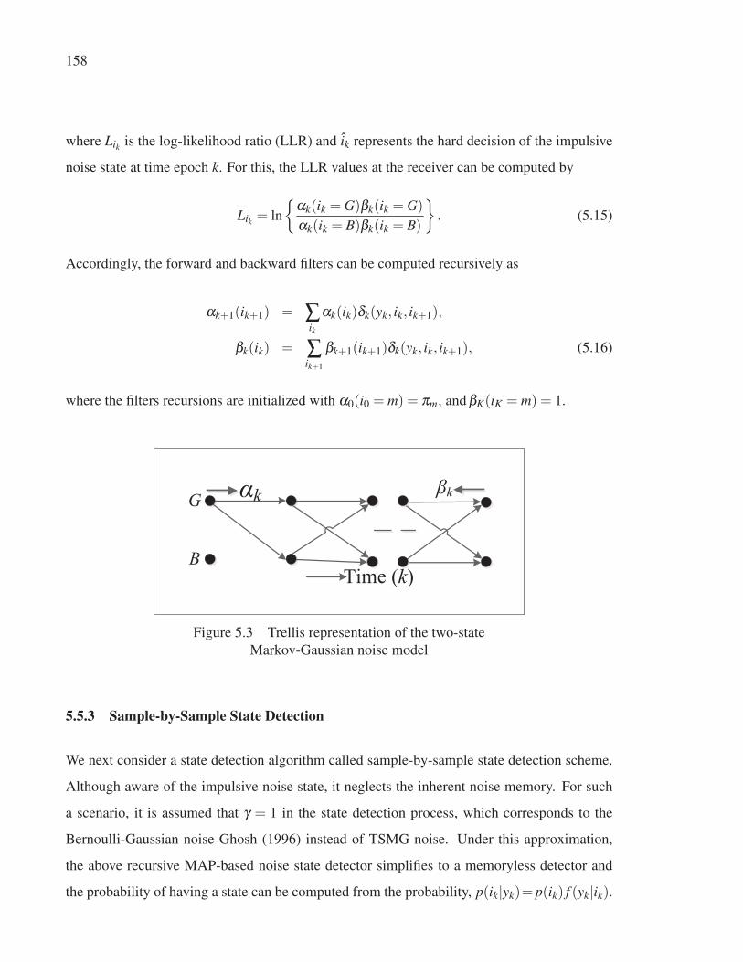
158

where Lik is the log-likelihood ratio (LLR) and ik represents the hard decision of the impulsive

noise state at time epoch k. For this, the LLR values at the receiver can be computed by

Lik = ln

{αk(ik = G)βk(ik = G)

αk(ik = B)βk(ik = B)

}. (5.15)

Accordingly, the forward and backward filters can be computed recursively as

αk+1(ik+1) = ∑ik

αk(ik)δk(yk, ik, ik+1),

βk(ik) = ∑ik+1

βk+1(ik+1)δk(yk, ik, ik+1), (5.16)

where the filters recursions are initialized with α0(i0 = m) = πm, and βK(iK = m) = 1.

G

BTime (k)

αk βk



5.5.3 Sample-by-Sample State Detection

We next consider a state detection algorithm called sample-by-sample state detection scheme.

Although aware of the impulsive noise state, it neglects the inherent noise memory. For such

a scenario, it is assumed that γ = 1 in the state detection process, which corresponds to the

Bernoulli-Gaussian noise Ghosh (1996) instead of TSMG noise. Under this approximation,

the above recursive MAP-based noise state detector simplifies to a memoryless detector and

the probability of having a state can be computed from the probability, p(ik|yk)= p(ik) f (yk|ik).

159

Using this, the LLR values are obtained as

Lik = ln

{πG f (yk|ik = G)

πB f (yk|ik = B)

}. (5.17)

Where f (yk|ik = m) = fG(yk;0,σ2s +σ2

m). From the LLR values, the receiver then determines

the noise states according to (5.14).

5.5.4 AWGN Scenario

This is the simplest estimation technique since it is blind to the noise states for the estimation

process. Under this consideration, the OBE sk(yk) of sk given yk can be obtained as

sk(yk) =σ2

sσ2

s +σ2n

yk. (5.18)

where σ2n = ∑m∈(G,B)πmσ2

m denotes the variance of n.

5.5.5 Complexity Discussion

It is worth to point out that, despite having a better performance, the complexity of the proposed

MAP-based MMSE estimation scheme grows exponentially with the frame length, due to the

implementation of the BCJR algorithm, while it grows linearly in case of symbol-by-symbol

estimation schemes Fertonani et al. (2007). However, in Section 5.7 we show that the potential

performance gain of this scheme justifies the increase in complexity, which makes this receiver

suitable for reliable communication scenarios. On the other hand, if we only consider the for-

ward recursions of the BCJR algorithm, then the complexity problem will probably be reduced

with a compromise in its performance. Hence, this scheme exhibits a performance/complexity

trade-off.

160

5.6 Performance Analysis

The performance of this scheme is evaluated in terms of distortion or MSE and it can be ob-

tained by

D ≡ E{(sk − sk)

2}=∫

s

∫y(sk − sk(yk))

2 f (s,y)dsdy, (5.19)

However, the closed form expression of the integrals in (5.19) is mathematically intractable

which makes it difficult to analytically investigate the MSE. As a result, approximating its

bounds remain an alternative solution to evaluate the performance of our proposed scheme. In

this vein, a lower bound (LB) is obtained under the hypothetical assumption that there is no

uncertainty about the state ik, i.e., the genie condition. The LB (DLB) under this consideration

can be obtained as

DLB = ∑m∈(G,B)

πm

(σ2

s −σ4

sσ2

s +σ2m

). (5.20)

To derive the upper bound (DUB), we invoke the LMMSE estimator since this latter obtains the

smallest MSE among all the estimators which are linear in the observations Kay (1993). The

MSE of the LMMSE estimator for this scheme is

DUB = σ2s −

σ4s

σ2s +σ2

n. (5.21)

5.7 Numerical Results

In this section, we simulate the MSE performances of the proposed scenario to confirm the ana-

lytical results. It is required to estimate the source parameter sk, which is modeled as a Gaussian

random variable, with variance σ2s = 1. Also, the impulsive noise that corrupts the source sig-

nal is characterized by the parameters πB = 0.1, γ = 100, and R = 100 Fertonani & Colavolpe

(2009). The MSE performances are calculated against average SNR. Here, the average SNR is

defined as SNR= σ2s /σ2

n .

161

-25 -20 -15 -10 -5 0 5 10 15 20

-20

-15

-10

-5

0

SNR [dB]

MSE

[dB]

MSE-Lower BoundMSE-Upper BoundMSE-Genie-Sim.MSE-MAP-Sim.MSE-MAP-forward-Sim.MSE-Sample-by-sample-Sim.MSE-AWGN-Sim

Figure 5.4 Analytical and simulated MSE performances of

different estimation techniques against the SNR. It is assumed that

πB = 0.1, R = 100, and γ = 100

Fig. 5.4 shows the simulated MSE performances of different estimation techniques. The simu-

lated MSE performances are obtained by calculating the sample means of (sk−sk(yk))2 using

2×105 frames with K=103 samples of each frame. In Fig. 5.4, the simulation result attained

under genie aided estimation perfectly matches the lower bound is well displayed. However,

the genie detection is practically infeasible. Interestingly, from the figure, it is also observed

that the proposed MAP-based MMSE estimator almost approaches the performance of ge-

nie aided scheme and performs significantly better than the conventional schemes. It obtains

a minimum SNR gain of around 8 dB over the LMMSE estimator and around 5 dB over the

sample-by-sample estimator, at the expense of a higher complexity, due to the BCJR algorithm.

Moreover, by considering the forward recursions of the BCJR algorithm, a tight performance

gap with the original scheme is observed, while the complexity problem is reduced. This con-

firms that significant performance gains can be obtained when the noise memory is utilized in

the estimation process. In addition, simpler sample-by-sample-based estimator still exhibits

better performance than the LMMSE scheme, by utilizing the impulsive noise statistics in the

estimation process. Finally, the LMMSE leads to the worst performances.

162

-20 -10 0 10

-10

-8

-6

-4

-2

0Memoryless channel

SNR [dB]

MSE

[dB]

-20 -10 0 10

-10

-8

-6

-4

-2

0AWGN channel

SNR [dB]

MSE

[dB]

MSE-MAP-Sim.MSE-Memoryless-Sim.MSE-AWGN-Sim.

MSE-MAP-Sim.MSE-Memoryless-Sim.MSE-AWGN-Sim.

Figure 5.5 MSE performances of different estimation techniques

against the SNR. It is assumed that πB = 0.1 with γ = 1, R = 100

for the memoryless channel, and γ = 1, R = 1 in case of AWGN

channel

Fig. 5.5 also shows the simulated MSE performances of different estimation techniques. The

essence of plotting Fig. 5.5 is to visualize how the proposed MAP-based MMSE estimator be-

haves over the memoryless and AWGN channel. From Fig. 5.5, it can be inferred that both the

MAP-based and sample-by-sample-based estimations show the same performance, when we

consider γ = 1 in the noise process. These results confirm that the optimal MAP detector sim-

plifies to the memoryless detector when the considered impulsive noise is memoryless. Again,

the LMMSE estimator attains around 5 dB worse performance over them in these impulsive

environments, in low SNR region. Finally, the three estimators obviously exhibit the same

performance over AWGN channel.

5.8 Conclusion

In this letter, we have provided the necessary theoretical foundation for optimal Bayesian esti-

mation of a scalar Gaussian source, in the presence of bursty impulsive noise. It is shown that

163

the presence of bursty impulsive noise makes the input-output characteristics of MMSE OBE

non-linear. To combat the effect of non-linearity, we have proposed a novel estimation tech-

nique based on detecting the unobservable states of the noise process. The simulation results

confirmed that the proposed MAP-based Bayesian MMSE estimator outperforms the various

MMSE estimators employing memoryless estimation. Noteworthy, the proposed estimator can

be easily adapted to any Gaussian source estimation in the presence of any Gaussian mixture

noise with memory. Future extension of this work may include deriving the exact closed form

expression for the MSE.

CHAPTER 6

PERFORMANCE ANALYSIS OF DISTRIBUTED WIRELESS SENSORNETWORKS FOR GAUSSIAN SOURCE ESTIMATION IN THE PRESENCE OF

IMPULSIVE NOISE




Article published in IEEE Signal Processing Letters, June, 2018.

6.1 Abstract

We address the distributed estimation of a scalar Gaussian source in wireless sensor networks

(WSNs). The sensor nodes transmit their noisy observations, using the amplify-and-forward

relaying strategy through coherent multiple access channel to the fusion center (FC) that re-

constructs the source parameter. In this letter, we assume that the received signal at the FC

is corrupted by impulsive noise and channel fading, as encountered for instance within power

substations. Over Rayleigh fading channel and in presence of Middleton class-A impulsive

noise, we derive the minimum mean square error (MMSE) optimal Bayesian estimator along

with its mean square error (MSE) performance bounds. From the obtained results, we conclude

that the proposed optimal MMSE estimator outperforms the linear MMSE estimator developed

for Gaussian noise scenario.

6.2 Introduction

The difficulty of estimating a Gaussian source from its available noisy measurements is preva-

lent in numerous signal processing contexts. In this aspect, over the past few years, researches

on the implementation of distributed WSN has been evolving very rapidly. For example, the

authors in Xiao, J.-J., Cui, S., Luo, Z.-Q. & Goldsmith, A. J. (2008) considered the distributed

166

estimation of scalar source parameters using a collaborative WSN. It is shown that depending

on the available information about the source statistics and the noise behaviour, different es-

timators can be used to achieve the MSE criterion. Similar performance analyses are carried

out in Aysal, T. C. & Barner, K. E. (2008); Cui, S., Xiao, J.-J., Goldsmith, A. J., Luo, Z.-

Q. & Poor, H. V. (2007); Wang, C.-H., Leong, A. S. & Dey, S. (2011a) to show the optimality

of the maximum likelihood estimator (MLE) Aysal & Barner (2008), best linear unbiased es-

timator (BLUE) Cui et al. (2007), and the MMSE estimator Wang et al. (2011a) based on the

available information about the source statistics.

However, all of the above performance analyses for distributed estimation schemes have been

carried out over the Gaussian noise scenario. On the other hand, the noise characteristics, usu-

ally observed in many environments, such as the power transmission lines areas, the power

substations, and in some mobile radio scenarios, are inherently impulsive in nature Middleton

(1977). For example, in power substations, the noise emitted from various power equipment are

impulsive Madi, G., Sacuto, F., Vrigneau, B., Agba, B. L., Pousset, Y., Vauzelle, R. & Gagnon,

F. (2011). In this context, the impacts of impulsive noise have been widely investigated on the

detection of finite alphabets in point-to-point and collaborative WSN communications Alam

et al. (2016); Spaulding & Middleton (1977). However, the performance of estimation tech-

niques in the presence of impulsive noise is not widely acknowledged.

Recently, the authors in Banelli (2013) considered the MMSE optimal Bayesian estimation

(OBE) for a Gaussian source impaired by Middleton class-A impulsive noise. It is shown that

the performance of the proposed MMSE OBE strictly depends on the statistical characteristics

of the received signal. The authors in Flam et al. (2012) derived the MMSE OBE and its MSE

performance bounds in closed form assuming that the noise and the source signals are Gaussian

mixture (GM) distributed. The obtained results showed that the performance improvement of

the optimal MMSE estimator over the linear MMSE (LMMSE) estimator under this condition

is substantial. However, the analyses in Banelli (2013); Flam et al. (2012) are restricted to

the point-to-point scenario and the effect of channel fading is not considered. To the best

of authors knowledge, no result exists for the distributed estimation of Gaussian sources in

167

the presence of impulsive noise under Rayleigh fading. Here, we provide a mathematical

framework for the performance analysis of distributed estimation of a scalar Gaussian source

impaired by Middleton class-A noise. A Middleton class-A process is a simple and effective

way to model an impulsive noise channel Banelli (2013); Middleton (1977). Our work is an

extension of Banelli (2013) to the distributed WSN scenario. It is assumed that each sensor

node transmits its observations to the FC through a coherent multiple access channel (MAC)

using AF strategy. It is widely acknowledged that AF schemes significantly outperform the

traditional source-channel coding for Gaussian signal estimation while preserving the sensor’s

radios low complexity Gastpar, M. & Vetterli, M. (2003). The FC uses the received signal to

estimate the source parameter with minimum MSE.

The contributions of this work are as follows. First, we derive the MMSE OBE for a scalar

Gaussian source estimation using distributed WSN in the presence of impulsive noise under

Rayleigh fading. It is seen that the presence of impulsive noise makes the input-output char-

acteristics of MMSE OBE non-linear especially when the environment is more impulsive, as

indicated by the rare impulsive events. This leads to a non-linear MMSE estimator. Then,

we provide upper and lower bounds for its MSE performance. Finally, the derived bounds are

validated through the Monte Carlo simulation. Interestingly, from the obtained results, it is

seen that the proposed optimal MMSE estimator attains the lower bound for highly impulsive

noise environment and performs significantly better than the LMMSE estimator developed for

AWGN scenario.

168

6.3 System model

S1+

+

+

+

S2

S3

SM

s FC+

n1

n2

n3

nM

h1h2

h3

hM

x1

x2

x3

xM

a1

a2

a3

aM

X

X

X

X

g1

g2g3

gM

ϑ z s

Figure 6.1 Distributed WSN for Gaussian source estimation

As shown in Fig. 6.1, we consider a WSN of M sensor nodes from S1 to SM and a FC. The

sensor nodes observe a scalar parameter s, which is modeled by a Gaussian random variable

(rv) with mean μs and variance σ2s . Let the signals measured by the ith sensor node, i =

1,2, . . . ,M, can be expressed as

xi = his+ni, (6.1)

where hi and ni denote the channel coefficient and the measurement noise at the ith sensor node,

respectively. In this work, as usual, the measurement noise variables {ni}Mi=1 are assumed to be

Gaussian with mean μn and variance σ2n . Now, the sensor nodes follow two-hop collaborative

communications to send the data from the source to the destination using AF strategy. In the

first hop, the sensor nodes measure the data of the source to be estimated and in the second

hop, each sensor node amplifies its measured signal xi by a factor of ai and transmits it to the

FC through a coherent MAC channel Xiao et al. (2008). The received signal, z, at the FC is

then given by

z =M

∑i=1

giaixi +ϑ , (6.2)

169

where gi is the channel coefficient between the ith sensor node and the FC, and ϑ is the com-

munication noise. We assume that the channel coefficients follow the Rayleigh distribution and

for each link, they are considered to be static for one symbol duration, while they vary from

one symbol to another. Therefore, both hi and gi are modeled by a zero-mean independent, cir-

cularly symmetric complex Gaussian random variable with variances σ2h and σ2

g , respectively.

It is assumed that the channel coefficients are known at both the transmitters and receiver side.

Hence, the signals can be added coherently at the FC Xiao et al. (2008). It is also assumed that

ϑ follows Middleton class-A distribution to account for impulsive communication disturbance.

Hence, the probability density function (PDF) of ϑ is given by Middleton (1977)

f (ϑ) =∞

∑m=0

pm√2πσm

exp

(− ϑ 2

2σ2m

), (6.3)

where pm = e−AAm

m! is the steady state probability of the mth impulsive source and σ2m =σ2

ϑm/A+Γ

1+Γ

is the variance of that impulsive source. For m = 0, the model generates the traditional AWGN

component. Also, the parameters A, Γ, and σ2ϑ are called the global parameters as they charac-

terize the PDF Middleton (1977). The physical significance of these parameters are: A denotes

the impulsive index, Γ indicates the Gaussian to impulsive noise power ratio, and σ2ϑ represents

the total power of the noise ϑ .

6.4 MMSE Optimal Bayesian Estimation

In this section, we consider the MMSE OBE of a scalar Gaussian source s impaired by Middle-

ton class-A noise under Rayleigh fading. The MMSE OBE corresponds to the posteriori mean

Kay (1993) and is given by

s = ε (s|z) ==∫

s f (s|z)ds, (6.4)

where s indicates the MMSE estimation of s and ε is the expectation operator. From equation

(6.4), we can deduce that the posteriori probability f (s|z) is required to derive the MMSE esti-

mator. Although the distribution of f (s|z) already exists for AWGN channel Xiao et al. (2008),

170

here, we derive the distribution for impulsive noise scenario. Now, (6.2) can be rearranged as

z = gT Whs+gT Wn+ϑ = αs+β , (6.5)

where g = [g1, . . . ,gM]T , h = [h1, . . . ,hM]T , W = diag(a) with a = [a1, . . . ,aM]T , and n =

[n1, . . . ,nM]T . Here, the amplification factor for each node is ai =√

(PT/M(σ2h σ2

s + σ2n )),

where PT is the total transmission power of all the sensor nodes. Also, α = gT Wh and

β = gT Wn+ϑ . It is assumed that N = gT Wn and ϑ are mutually independent with each

other. Then, from the convolution property, the distribution of β is represented by

f (β ) =∞

∑m=0

pmN (β ,μβ ,σ2β ,m) (6.6)

where N (β ,μβ ,σ2β ,m) is a Gaussian random variable with mean μβ = gT Wμn and variance

σ2β ,m = gT WσNWT g+σ2

m, σN = ε{

nnT}. Moreover, s and β are mutually independent. Then,

the joint distribution of s and β is given by

f (s,β ) = f (s)× f (β ) =∞

∑m=0

pmN (s,β ,μm,σm), (6.7)

where μm =[μs μβ

]and σm =

[σ2

s 0;0 σ2β ,m

]. Now, from equation (6.5) we have,

⎡⎣ z

s

⎤⎦=

⎡⎣ αs+β

s

⎤⎦=

⎡⎣ α I

I 0

⎤⎦⎡⎣ s

β

⎤⎦= C

⎡⎣ s

β

⎤⎦ , (6.8)

It is well known that if s and β are jointly Gaussian, then z and s will also be jointly Gaussian,

since the linear transformation of a Gaussian vector is Gaussian too (Kay, 1993, pg. 325).

However, it holds for GM also and hence [z,s]T = C[s,β ]T is also jointly GM with Flam et al.

(2012)

f (z,s) =∞

∑m=0

pmN (z,s,Cμm,CσmCT ), (6.9)

171

where,

Cμm =

⎡⎣ α I

I 0

⎤⎦⎡⎣ μs

μβ

⎤⎦=

⎡⎣ αμs +μβ

μs

⎤⎦=

⎡⎣ μm

z

μs

⎤⎦ , (6.10)

and

CσmCT =

⎡⎣ ασ2

s αT +σ2β ,m ασ2

s

σ2s αT σ2

s

⎤⎦=

⎡⎣ σ2

z,m σ2zs

σ2sz σ2

s

⎤⎦ . (6.11)

Now, from the joint distribution of (6.9), the conditional PDF of s given z can be evaluated as

f (s|z) = f (s,z)f (z)

=∞

∑m=0

χm(z)N (s,μms|z(z),Σ

ms|z(z)). (6.12)

Where the third equality comes from (Kay, 1993, Theorem 10.3) and considering

χm(z) =pmN (z,μm

z ,σ2z,m)

∑∞m=0 pmN (z,μm

z ,σ2z,m)

. (6.13)

Using (Kay, 1993, Theorem 10.3), we can write

μms|z(z) = μs +

σ2s hT WT g

gT Whσ2s hT WT g+gT WσNWT g+σ2

m

(z−μm

z)

(6.14)

and,

Σms|z(z) = σ2

s −σ2

s hT WT ggT Whσ2s


m. (6.15)

Hence, using equation (6.4) and (6.12), the MMSE estimation of s given z is obtained by

s =∫

s∞

∑m=0

χm(z)N (s,μms|z(z),Σ

ms|z(z))ds,

=∞

∑m=0

χm(z)μms|z(z). (6.16)

Where χm(z) and μms|z(z) are defined in (6.13) and (6.14), respectively. Equation (6.16) high-

lights how the MMSE OBE depends on the signal, noise, and channel parameters for the pro-

posed scenario. In the special case of when both ni and ϑ are Gaussian as in Xiao et al. (2008),

172

the corresponding MMSE estimation of s given z is given by

s =σ2

s hT WT ggT Whσ2

s hT WT g+gT WσNWT g+σ2ϑ

z. (6.17)

Which is equivalent to the expression in (Xiao et al., 2008, pp. 760). It should also be noted

that (6.16) is equivalent to the expression of the OBE in (Banelli, 2013, eqn. (8)) in the special

case of when μs = 0 and z is the measurement, for a point-to-point scenario.

6.4.1 Distortion Analysis

The distortion of this scheme is evaluated in terms of MSE and it can be obtained by

D ≡ ε{(s− s)2

}=∫

s

∫z

(s−μs|z

)2 f (s,z)dsdz, (6.18)

=∫

s

∫z

(s−μs|z

)2 f (s|z) f (z)dsdz (6.19)

=∫

zΣs|z f (z)dz,

where the posteriori covariance Σs|z can be obtained as derived in Flam et al. (2012)

Σs|z =∞

∑m=0

χm(z)(

Σms|z +

(μm

s|z)2)− (

μs|z)2. (6.20)

Hence, from equation (6.20) we have

D =∫

z

∞

∑m=0

χm(z)(

Σms|z +

(μm

s|z)2 − (

μs|z)2)

f (z)dz,

=∞

∑m=0

pm

∫z

(Σm

s|z +(

μms|z)2 − (

μs|z)2)

fm(z)dz, (6.21)

where fm(z) = N (z,μmz ,σ2

z,m). However, equation (6.21) is similar to the expression in (Flam

et al., 2012, eqn. (21)) and can not be solved analytically. Hence, we may derive its bounds.

In this vein, a lower bound (LB) is obtained under the hypothetical assumption that there is

no uncertainty about the impulsive component m and the Rayleigh channel state information,

173

i.e., the genie condition. Following the same procedure as in Flam et al. (2012), the LB (DLB)

under this consideration can be obtained as

DLB =∞

∑m=0

pmΣms|z(z). (6.22)

Where Σms|z(z) is defined in (6.15). To derive the upper bound (DUB), as in Flam et al. (2012),

we invoke the LMMSE estimator since the LMMSE obtains the smallest MSE among all the

estimators which are linear in the observations Flam et al. (2012). The MSE of the LMMSE

estimator for this scheme is

DUB = σ2s −

σ2s hT WT ggT Whσ2

s


ϑ. (6.23)

6.5 Numerical Results

In this section, the performance of MMSE optimal Bayesian estimator and distortion parameter

bounds are evaluated under AWGN, and Middleton class-A noise over Rayleigh quasi-static

flat fading channel with respect to the communication signal-to-noise ratio (SNR). Here, the

communication SNR is defined as σ2h σ2

s +σ2n/σ2

ϑ and the measurement SNR asσ2s /σ2

n =0 dB,

where σ2s = 1. In this model, a total number of 10 sensor nodes transmit with equal power

their observations to the FC using AF strategy. The total transmission power of all the sensor

nodes is PT = 1 dB. Moreover, the channel fading have variances σ2h =σ2

g =1. The Middleton

class-A model has the total number of impulsive sources which is equal to 30 and Γ=0.01. As

in Banelli (2013), it is assumed that the impulsive noise parameters are known at the receiver

side.

Fig. 6.2 shows the input-output characteristics of MMSE OBE using equation (6.16) for differ-

ent values of the impulsive index A. As observed in Fig. 6.2, when the value of A increases, the

impulsive noise becomes closer to the Gaussian noise and the input-output characteristics of

MMSE OBE tend to the well-known LMMSE estimation which is optimal in the case of Gaus-

174

sian noise. On the other hand, when the value of A decreases, the environment becomes more

impulsive as indicated by rare impulsive events and the input-output characteristic becomes

more non-linear. Thus, similar to point-to-point scenario, the presence of impulsive noise in-

troduce non-linearity in the measurement z. Hence, the MMSE optimal Bayesian estimator

becomes non-linear under that scenario.

-20 -15 -10 -5 0 5 10 15 20-6

-4

-2

0

2

4

6

z

s MM

SE (z

)

A=0.001A=0.1A=1A=10AWGN

Figure 6.2 Impact of the impulsive index A on the input-output

characteristics of MMSE optimal Bayesian estimation. It is

assumed that both the measurement SNR and the communication

SNR are equal to 0 dB

To visualize the effect of the non-linearity, we also have plotted the distortion performance

for the proposed scenario. Fig. 6.3 shows the simulated MSE performances of the optimal

MMSE estimation along with its derived analytical upper and lower bounds for different values

of the impulsive index A. The simulated MSE performance is obtained by calculating the

sample-mean of (s− μs|z)2. From Fig. 6.3, it is seen that at both low and high SNR values

the MMSE performs as the LMMSE (upper bound) estimator. However, at intermediate SNR

levels, the MMSE estimator performs significantly better than the LMMSE estimator by using

the impulsive noise characteristics in the estimation process and the amount of improvement

175

depends on the impulsive nature as indicated by different values of A. From Fig. 6.3, it is

further confirmed that as the value of A increases, the nature of impulsive noise becomes more

Gaussian and the MSE performance of MMSE estimator approaches to the LMMSE estimator

for all SNR values. Under this situation, the performance gap between the lower and the upper

bounds decreases and approaches to zero for sufficiently larger values of A. On the other hand,

for small values of A, the impulses are less dominant (more impulsive) and the performance

gap between the upper and lower bounds becomes larger. The MMSE estimator approaches

the lower bound under this scenario. Interestingly, when the impulsive events are very rare, the

MMSE converges to the lower bound. Hence, the derived lower bound is very tight for highly

impulsive noise environments.

-40 -30 -20 -10 0 10 20 30 40-9

-8

-7

-6

-5

-4

-3

-2

-1

0

Communication SNR [dB]

MSE

[dB]

. . . . - - - -

- -. .

A = 10A = 1

A = 0.1A = 0.01no line A = 0.001

MSE - Lower BoundMSE - SimulationMSE - Upper Bound

*

Figure 6.3 Impact of the impulsive index A on the

distortion performance. It is assumed that the measurement

SNR is equal to 0 dB

Lastly, Fig. 6.4 shows the simulated MSE performances of the proposed system as a function of

the total number of sensor nodes under different values of the impulsive index A. From Fig. 6.4,

it is seen that similar to Gaussian case, the distortion performance decreases exponentially

as the value of M increases while keeping the total transmission power constant. Also, for

176

sufficiently large value of M the performance of the proposed non-linear MMSE estimator

converges with the LMMSE estimator irrespective of the value of A.

0 100 200 300 400 500-20

-15

-10

-5

0

Total number of sensor nodes (M)

MSE

[dB]

A=1A=0.1A=0.01LMMSE

Figure 6.4 Plot of distortion versus the total number of

sensor nodes under different values of impulsive index A. It is

assumed that both the measurement SNR and the

communication SNR are equal to 0 dB

6.6 Conclusion

WSN consists of spatially distributed sensors, identified as a promising technology for un-

known parameters estimations. In this letter, the distributed estimation of a scalar Gaussian

source in WSNs in the presence of Middleton class-A noise is considered. For this scheme, a

closed-form expression for the MMSE optimal Bayesian estimation and the upper and lower

bounds for the MSE are derived to show the effect of impulsive noise. It is shown that the per-

formance improvement of the derived optimal MMSE estimator over the LMMSE estimator

depends on the impulsive nature of the noise and on the operating SNR regions.

CHAPTER 7

CONCLUSION AND RECOMMENDATIONS

7.1 Conclusion

It is well-known that the most significant amount of GHG emissions (mostly carbon dioxide)

all around the world in recent years came from the electricity sector. This is because there is an

increase in electricity consumption due to the increasing rate of population and industrialization

whereas power systems mainly use fossil fuels for electricity generation. To avert the severe

impacts of climate change on human and natural systems, carbon dioxide (CO2) emissions

from the electric power sector must rapidly decrease. One solution to reduce GHG emissions

from electricity generation is to modernize the power grid, in which ICTs are playing a key

role. Indeed, this novel concept has emerged to manage the increasing demand for energy

resources while maintaining the CO2 emission at a certain level by enhancing the energy usage

efficiency. The electric power research institute (EPRI) found that a full deployment of a smart

grid and the new technologies that it enables can reduce GHG emissions by 13% - 25%. Other

possible potential benefits of the smart grid applications include decreasing blackouts, ensuring

safer and more secure delivery of electricity, lowering the power cost by giving more control

over the power use, reducing expenses for energy production, increasing grid visibility, and

more significantly making Canada’s energy autonomous.

For a reliable smart grid, monitoring and control of power system parameters in the transmis-

sion and distribution segments as well as the substation devices is crucial. In order to allow

such advanced functionalities and avoid possible disruptions in electric systems due to unex-

pected failures, a highly reliable, scalable, secure, cost-effective, and robust communication

network must be operational within the power grid that conveys data from monitoring sensors

in the field back to engineers in the control room. In this vein, the most promising method of

smart grid communication explored in the literature is based on WSNs due to their inherent

characteristics of being low-cost and flexible as well as their wider coverage, self-organization

178

and rapid deployment. Also, it circumvents the typical constraints associated with the instal-

lation of wired communication systems. Therefore, considerable efforts have been given to

design a stable and efficient WSN for smart grid communications since the beginning of smart

grid projects. However, harsh and complex electric power system environments pose great

challenges on the reliability of wireless sensor nodes communications because of obstructions,

strong RF interference, and noise. More specifically, the noise characteristics that are usually

observed in smart grid scenarios are highly non-Gaussian and are inherently impulsive in na-

ture. Impulsive noise degrades the system performance significantly because its spectrum is

more powerful than the Gaussian noise. Also, the impulsive noise measurement campaigns in

smart grid environments show that the impulses occur in bursts. Hence conventional WSNs

explored in the literature for smart grid communication showed poor performance under such

scenarios.

Therefore, the main research goal of this dissertation is to lay down the fundamental basis

for the development of a robust and efficient WSN for smart grid communication to realize

real-world smart grid applications. With this aim in mind, conclusively speaking, there are

three main aspects of this dissertation: (i) investigation and performance analysis of impulsive

noise mitigation techniques for point-to-point single-carrier communication systems impaired

by bursty impulsive noise; (ii) design and performance analysis of a collaborative WSN for

smart grid monitoring by considering the RF noise model in the design process, a particular in-

tension is given to how the time-correlation among the noise samples can be taken into account;

(iii) optimal MMSE estimation of physical parameters like the temperature, current, voltage,

etc., typically modeled by a scalar Gaussian source in the presence of impulsive noise.To be

specific, the aforementioned contributions are further detailed as follows:

- The first aspect of this dissertation (Chapter 2) evaluated some practical impulsive noise

mitigation techniques for LDPC coded single-carrier point-to-point communication systems

subject to bursty impulsive noise modelled by a Markov-Gaussian process. The provided

simulation results showed that the LLR-based impulsive noise mitigation technique with the

179

MAP detection criterion outperforms the simple but more popular clipping, blanking, and

combined clipping/blanking schemes at the expense of higher computational complexity.

- The second aspect of this dissertation contains two sub-contributions and are provided in

Chapters 3 and 4, respectively. The performance analysis of a single relay DF collaborative

WSN scheme over channels impaired by bursty impulsive noise has been conducted in

Chapter 3. For this channel, the BER performances of DT and single relay collaborative

WSN schemes using M-PSK modulation in the presence of Rayleigh fading with a MAP

receiver are evaluated. From the obtained results, it is seen that the DF collaborative WSN in

bursty impulsive noise channels still achieves the space diversity and performs significantly

better than DT under the same power consumption. Moreover, the proposed MAP receiver

attains the lower bound derived for the DF collaborative WSN scheme, and leads to large

performance gains in terms of reliability compared to the conventional receiving criteria

which were optimized for the AWGN channel and the memoryless impulsive noise channel.

- As a continuation of the single relay collaborative WSN scheme in Chapter 3, a novel re-

lay selection protocol for a DF collaborative WSN taking into account the bursty impulsive

noise was proposed in Chapter 4. The proposed protocol chooses the N’th best relay con-

sidering both the channel gains and the states of the impulsive noise of the source-relay and

relay-destination links. For this scheme, to obtain the state of the impulsive noise, we pro-

pose a state detection algorithm using MAP detection. To analyze the performance of the

proposed protocol, we first derive closed-form expressions for the PDF of the received SNR

assuming all the relays know the state of impulsive noise perfectly. Then, these PDFs are

used to derive closed-form expressions for the BER and the outage probability. Finally, we

also derive the asymptotic BER and outage expressions to quantify the diversity benefits.

We show that the proposed MAP-based N’th BRS protocol attains the derived genie-aided

analytical results and outperforms the conventional relay selection protocol, optimized for

the Gaussian case, and which does not take into account the impulsive noise memory.

- The aforementioned chapters talked about the reliable detection of finite alphabets in the

presence of bursty impulsive noise. The performance of the optimal MMSE estimation for a

180

scalar Gaussian source impaired by impulsive noise has been conducted in Chapters 5 and 6,

respectively. In Chapter 5, the MMSE OBE for a scalar Gaussian source, in the presence of

bursty impulsive noise, as essentially encountered within power substations is considered.

Clearly, it is observed that the presence of bursty impulsive noise makes the input-output

characteristics of MMSE OBE non-linear. To handle the non-linearity, we propose a novel

MMSE estimator, based on the detection of the unobservable states of the noise process,

using the MAP detector. Resultantly, the proposed MAP-based MMSE estimator is shown

to achieve the lower bound derived for the proposed scenario and outperform the various

MMSE estimators that neglect the noise memory.

- On the other hand, in chapter 6, the distributed estimation of a scalar Gaussian source

in WSNs in the presence of Middleton class-A noise is considered. For this scheme, a

closed-form expression for the MMSE optimal Bayesian estimation and the upper and lower

bounds for the MSE are derived to show the effect of impulsive noise. It is shown that

the performance improvement of the derived optimal MMSE estimator over the LMMSE

estimator depends on the impulsive nature of the noise and on the operating SNR regions.

The achievement of this project is expected to facilitate the industrial implementation of col-

laborative WSN based smart grid communication systems that will help in achieving the target

of reducing Canada’s 2005 greenhouse gas emission by 30% by 2030.

7.2 Future work

The contributions presented in this dissertation could be extended to the following future re-

search directions:

7.2.1 Resource constraints of sensor nodes

In WSNs, all nodes are equipped with a battery and hence the sensor nodes applications are

constrained by a limited battery life. Replacing or charging the batteries in WSNs may take

time and be costly for a large number of sensors. This is particularly important for substation

181

and high voltage transmission line monitoring applications due to the relative inaccessibility

of the regions for safety and regulatory purposes. To solve the issue of limited battery life of

sensor nodes, many energy efficient protocols have been widely investigated in the literature

where various energy-efficient medium access and routing protocols and duty-cycling have

been considered. However, these techniques are able to provide only limited lifetime Erol-

Kantarci & Mouftah (2012). On the other hand, energy harvesting methods play an important

role in the lifetime of WSNs. By harvesting the energy from the ambient resources it is possible

to extend the lifetime of the sensor nodes. In particular, RF signals can concurrently carry

information and energy signals, also known as simultaneous wireless information and power

transfer (SWIPT), which has attracted significant research interest recently Kaddoum, G., Tran,

H.-V., Kong, L. & Atallah, M. (2016b); Tran, H.-V., Kaddoum, G. & Truong, K. T. (2018);

Zhou, X., Zhang, R. & Ho, C. K. (2013). However, most existing works on this topic assume

negligible background noise power. The performance of wireless energy harvesting systems

with consideration of the practical impulsive noise environments is worthwhile to be examined

and analyzed in the future research directions.

7.2.2 Effect of Network Geometry/Nodes’ Locations Distributions

A typical WSN consists of a large number of sensor nodes deployed in an area of interest to

collect specific information about the surrounding environment. In our previous works, it is

assumed that the sensor nodes’ locations are known. However, in most cases of WSNs appli-

cations, the sensor nodes are distributed randomly and it is hard to know the locations of the

sensor nodes’ due to harsh geographic conditions which is exactly the case in smart grid appli-

cations. In such cases, the nodes’ locations distribution can be modeled by a two-dimensional

Poisson point process (PPP) Haenggi, M. (2005); Sattar, Z., Evangelista, J. V. D. C., Kaddoum,

G. & Batani, N. (2019). As a result, how the sensor nodes’ locations distribution affects the

performance will be a promising direction.

182

7.2.3 Security

The wireless nature of WSNs also makes WSN-based smart grid applications vulnerable to

various external attacks, physical and cyber threats. Hence, security is an essential issue in

the design of WSN-based smart grid communications in order to securely transmit the data

from the end-users to the data collection centers. In addition to cyber security issues that have

been widely investigated in the literature since the beginning of smart grid projects, one may

also analyze the physical layer security aspects that have been hardly investigated in the smart

grid scenario Atallah, M. & Kaddoum, G. (2019); Atallah, M., Alam, M. S. & Kaddoum, G.

(2019); Jameel, F., Wyne, S., Kaddoum, G. & Duong, T. Q. (2018); Lee et al. (2012). How

the performance of the later aspect can be improved by designing new advanced algorithms to

satisfy smart grid scenarios needs further investigation.

7.2.4 Imperfect knowledge of noise parameters

As presented in the whole thesis, it is assumed that the availability of noise parameters are per-

fectly known at the receiver. Such an assumption is practically challenging in some scenarios.

Towards this end, how to elaborate the influences led by the uncertainty of the noise parameters

will be a promising direction.

183

APPENDIX I

PROOF FOR CHAPTER 4

Derivation of the Marginal PDF: Asymptotic case

In the high SNR regime, it is assumed that 1− e−x .= x. Then, from (4.27), we have

I1.= M

(M−1

N −1

)1

γSRmγRmD

e− x

γSRm

(1

γa

)M−N ∫ x

z=0zM−Ne

− zγRmD dz, (A -1)

Assuming zγRmD

= q, (A -1) can be rearranged as

I1 =CM

γSRmγRmD

e− x

γSRm

(1

γa

)M−N ∫ xγRmD

z=0qM−Ne−qdq,

=CM

γSRm

e− x

γSRm

(1

γa

)M−N

γ(M−N +1,x

γRmD), (A -2)

where γ(a,b) is the lower incomplete gamma function. At high SNR scenario, x ≈ 0 and I1 can

be neglected. Again,

I2 =CM

γSRmγRmD

(xγa

)M−N

e− x

γSRm

∫ ∞

z=xe− z

γRmD dz,

= M(

M−1

N −1

)1

γSRm

(xγa

)M−N

e−x

γa , (A -3)

≈ M(

M−1

N −1

)1

γSRm

(1

γa

)M−N

xM−N . (A -4)

Substituting I1 and I2 in (4.27), yields (4.57).

REFERENCES

Agba, B. L., Sacuto, F., Au, M., Labeau, F. & Gagnon, F. (2019). Impulsive Noise Measure-

ments. In Wireless Communications for Power Substations: RF Characterization andModeling (pp. 35–68). Springer.

Ahmed, I., Nasri, A., Michalopoulos, D. S., Schober, R. & Mallik, R. K. (2012). Relay subset

selection and fair power allocation for best and partial relay selection in generic noise

and interference. IEEE Trans. Wireless Commun., 11(5), 1828–1839.

Akyildiz, I. F., Su, W., Sankarasubramaniam, Y. & Cayirci, E. (2002). Wireless sensor net-

works: a survey. Computer networks, 38(4), 393–422.

Al-Badarneh, Y. H., Georghiades, C. N. & Alouini, M.-S. (2018). Asymptotic Performance

Analysis of the k-th Best Link Selection Over Wireless Fading Channels: An Extreme

Value Theory Approach. IEEE Trans. Veh. Technol., 67(7), 6652–6657.

Al-Badarneh, Y. H., Georghiades, C. N. & Alouini, M.-S. (2019). On the Asymptotic Through-

put of the k-th Best Secondary User Selection in Cognitive Radio Systems. Proc. IEEEVeh. Technol. Conf., pp. 1–5.

Al-Dharrab, S. & Uysal, M. (2009a). Cooperative diversity in the presence of impulsive noise.

IEEE Trans. Wireless Commun., 8(9), 4730–4739.

Al-Dharrab, S. & Uysal, M. (2009b). Cooperative diversity over fading channels with impul-

sive noise. Proc IEEE Wireless Commun. Networking Conf., pp. 1–6.

Al-Naffouri, T. Y., Quadeer, A. A. & Caire, G. (2014). Impulse noise estimation and removal

for OFDM systems. IEEE Trans. Commun., 62(3), 976–989.

Alam, M. S. & Labeau, F. (2015a). Performance analysis of DF cooperative relaying over

bursty impulsive noise channel. IEEE Sixth International Conference on Smart GridCommunications(SmartGridComm’2015), pp. Accepted for publication.

Alam, M. S. & Labeau, F. (2015b). Performance analysis of DF cooperative relaying over

bursty impulsive noise channel. Proc. IEEE Int. Conf. Smart Grid Commun., pp. 374–

379.

Alam, M. S. & Labeau, F. (2016a). Effect of Bursty Impulsive Noise on the Performance of

Multi-relay DF Cooperative Relaying Scheme. Proc. IEEE Veh. Technol. Conf., pp. 1–5.

Alam, M. S. & Labeau, F. (2016b). On relay selection in bursty impulsive noise channel. Proc.IEEE Wireless Commun. Networking Conf., pp. 1–6.

186

Alam, M. S., Labeau, F. & Kaddoum, G. (2016). Performance analysis of DF cooperative

relaying over bursty impulsive noise channel. IEEE Trans. Commun., 64(7), 2848–2859.

Alam, M. S., Kaddoum, G. & Agba, B. (2018a). Performance analysis of distributed wireless

sensor networks for Gaussian source estimation in the presence of impulsive noise. IEEESig. Proc. Letters, 25(6), 803–807.

Alam, M. S., Kaddoum, G. & Agba, B. L. (2018b). Bayesian MMSE estimation of a Gaussian

source in the presence of bursty impulsive noise. IEEE Commun. Letters, 22(9), 1846–

1849.

Alamouti, S. M. (1998). A simple transmit diversity technique for wireless communications.

IEEE J. Sel. Areas Commun., 16(8), 1451–1458.

Ali, I. B. S., Au, M., Agba, B. L. & Gagnon, F. (2015). Mitigation of impulsive interference

in power substation with multi-antenna systems. Proc. Int. Conf. Ubiquitous WirelessBroadband, pp. 1–5.

Arnold, D. M., Loeliger, H.-A., Vontobel, P. O., Kavcic, A. & Zeng, W. (2006). Simulation-

based computation of information rates for channels with memory. IEEE Trans. Inf.Theory, 52(8), 3498–3508.

Asiyo, M. O. & Afullo, T. J. (2017). Analysis of bursty impulsive noise in low-voltage indoor

power line communication channels: local scaling behaviour. SAIEE Africa Res. J.,108(3), 98–107.

Atallah, M. & Kaddoum, G. (2019). Design and Performance Analysis of Secure Multicas-

ting Cooperative Protocol for Wireless Sensor Network Applications. arXiv preprintarXiv:1902.07345.

Atallah, M., Alam, M. S. & Kaddoum, G. (2019). Secrecy Analysis of Wireless Sensor

Network in Smart Grid with Destination Assisted Jamming. IET Commun.

Aysal, T. C. & Barner, K. E. (2008). Constrained decentralized estimation over noisy channels

for sensor networks. IEEE Trans. Signal Process., 56(4), 1398–1410.

Aziz, A. A., Iwanami, Y. & Okamoto, E. (2009). Efficient combining technique with a low-

complexity detect-and-forward relay for cooperative diversity scheme. Proc. IEEE Re-gion 10 Conf., pp. 1–6.

Bahl, L., Cocke, J., Jelinek, F. & Raviv, J. (1974). Optimal decoding of linear codes for

minimizing symbol error rate. IEEE Trans. Inf. Theory, 20(2), 284–287.

Bai, T., Zhang, H., Zhang, R., Yang, L.-L., Al Rawi, A. F., Zhang, J. & Hanzo, L. (2017).

Discrete multi-tone digital subscriber loop performance in the face of impulsive noise.

187

IEEE Access, 5, 10478–10495.

Banelli, P. (2013). Bayesian estimation of a Gaussian source in Middleton’s class-A impulsive

noise. IEEE Signal Process. Lett., 20(10), 956–959.

Berrou, C., Glavieux, A. & Thitimajshima, P. (1993). Near Shannon limit error-correcting

coding and decoding: Turbo-codes. 1. Proc. IEEE Int. Conf. Commun., 2, 1064–1070.

Blackard, K. L., Rappaport, T. S. & Bostian, C. W. (1993). Measurements and models of

radio frequency impulsive noise for indoor wireless communications. IEEE J. Sel. AreasCommun., 11(7), 991–1001.

Bletsas, A., Khisti, A., Reed, D. P. & Lippman, A. (2006). A simple cooperative diversity

method based on network path selection. IEEE J. Sel. Areas Commun., 24(3), 659–672.

Brak, M. E., Brak, S. E., Essaaidi, M. & Benhaddou, D. (2014). Wireless Sensor Network

applications in smart grid. Proc. Int. Renewable and Sustainable Energy Conf., pp. 587–

592.

Changcai, H. & Weiling, W. (2008). Distributed generalized low-density codes for multiple

relay cooperative communications. EURASIP J. Wireless Commun. Net., 2008.

Cheffena, M. (2012). Industrial wireless sensor networks: channel modeling and performance

evaluation. EURASIP J. Wireless Commun. Net., 2012(1), 297.

Cheng, P., Wang, L., Zhen, B. & Wang, S. (2011). Feasibility study of applying LTE to Smart

Grid. Proc. First Int. Workshop Smart Grid Modeling and Simulation, pp. 108–113.

Cover, T. & Gamal, A. E. (1979). Capacity theorems for the relay channel. IEEE Trans. Inf.Theory, 25(5), 572–584.

Cui, S., Xiao, J.-J., Goldsmith, A. J., Luo, Z.-Q. & Poor, H. V. (2007). Estimation Diversity

and Energy Efficiency in Distributed Sensing. IEEE Trans. Signal Process., 55(9), 4683–

4695.

David, H. A. & Nagaraja, H. N. (2003). Order Statistics. Hoboken, NJ, USA: Wiley.

Erol-Kantarci, M. & Mouftah, H. T. (2011). Wireless sensor networks for smart grid applica-

tions. Proc. Saudi Int. Electronics, Commun. Photonics Conf., pp. 1–6.

Erol-Kantarci, M. & Mouftah, H. T. (2012). Suresense: sustainable wireless rechargeable

sensor networks for the smart grid. IEEE Wireless Commun., 19(3), 30–36.

Fadel, E., Gungor, V., Nassef, L., Akkari, N., Maik, M. A., Almasri, S. & Akyildiz, I. F. (2015).

A survey on wireless sensor networks for smart grid. Computer Communications, 71,

22–33.

188

Fang, X., Misra, S., Xue, G. & Yang, D. (2012). Smart grid−The new and improved power

grid: A survey. IEEE Commun. Surveys Tuts., 14(4), 944–980.

Fareed, M. M. & Uysal, M. (2009). On relay selection for decode-and-forward relaying. IEEETrans. Wireless Commun., 8(7), 3341–3346.

Farhangi, H. (2010). The path of the smart grid. IEEE Power Energy Mag., 8(1), 18–28.

Ferreira, H., Lampe, L., Newbury, J. & Swart, T. (2010). Power Line Communications: theoryand Applications for Narrowband and Broadband Communications over Power Lines.

Wiley.

Fertonani, D. & Colavolpe, G. (2009). On reliable communications over channels impaired by

bursty impulse noise. IEEE Trans. Commun., 57(7), 2024–2030.

Fertonani, D., Barbieri, A. & Colavolpe, G. (2007). Reduced-complexity BCJR algorithm for

turbo equalization. IEEE Trans. Commun., 55(12), 2279–2287.

Flam, J. T., Chatterjee, S., Kansanen, K. & Ekman, T. (2011). Minimum mean square error

estimation under gaussian mixture statistics. arXiv e-print, 2011 [Oneline]. Available:arXiv:1108.3410.

Flåm, J. T., Jaldén, J. & Chatterjee, S. (2011). Gaussian mixture modeling for source localiza-

tion. Proc. IEEE Int. Conf. Acoust., Speech Signal Process., pp. 2604–2607.

Flam, J. T., Chatterjee, S., Kansanen, K. & Ekman, T. (2012). On MMSE estimation: A linear

model under Gaussian mixture statistics. IEEE Trans. Signal Process., 60(7), 3840–

3845.

Gastpar, M. & Vetterli, M. (2003). Source-channel communication in sensor networks. Proc.Inf. Processing Sensor Net., pp. 162–177.

Ghosh, M. (1996). Analysis of the effect of impulse noise on multicarrier and single carrier

QAM systems. IEEE Trans. Commun., 44(2), 145–147.

Goldsmith, A. (2005). Wireless communications. Cambridge university press.

Gungor, V. C. & Lambert, F. C. (2006). A survey on communication networks for electric

system automation. Computer Networks, 50(7), 877–897.

Gungor, V. C., Lu, B. & Hancke, G. P. (2010). Opportunities and challenges of wireless sensor

networks in smart grid. IEEE Trans. Ind. Electron., 57(10), 3557–3564.

Gungor, V. C., Sahin, D., Kocak, T., Ergut, S., Buccella, C., Cecati, C. & Hancke, G. P. (2011).

Smart grid technologies: communication technologies and standards. IEEE Trans. Ind.Informat., 7(4), 529–539.

189

Haas, Z. J., Halpern, J. Y. & Li, L. (2006). Gossip-based ad hoc routing. IEEE/ACM Trans.Networking, 14(3), 479–491.

Hadi, A., Rabie, K. M. & Alsusa, E. (2016). Polar codes based OFDM-PLC systems in the

presence of Middleton class-A noise. 10th International Symposium on CommunicationSystems, Networks and Digital Signal Processing, pp. 1–6.

Hadjtaieb, A., Chelli, A., Alouini, M.-S. & Boujemaa, H. (2014). Performance analysis of

selective decode-and-forward multinode incremental relaying with maximal ratio com-

bining. Proc. Int. Conf. Commun. Networking, pp. 1–6.

Haenggi, M. (2005). On distances in uniformly random networks. IEEE Trans. Inf. Theory,

51(10), 3584–3586.

Hikita, M., Yamashita, H., Hoshino, T., Kato, T., Hayakawa, N., Ueda, T. & Okubo, H. (1998).

Electromagnetic noise spectrum caused by partial discharge in air at high voltage substa-

tions. IEEE Trans. Power Del., 13(2), 434–439.

Hossain, E., Han, Z. & Poor, H. V. (2012). Smart Grid Communications and Networking.

Cambridge University Press.

Hunter, T. E. & Nosratinia, A. (2006). Diversity through coded cooperation. IEEE Trans.Wireless Commun., 5(2), 283–289.

Huynh, K. Q. & Aulin, T. (2012). Improved Iterative Decoders for Turbo-Coded Decode-and-

Forward Relay Channels. Proc. IEEE Int. Conf. Veh. Technol., pp. 1–5.

Ibrahim, A. S., Sadek, A. K., Su, W. & Liu, K. R. (2008). Cooperative communications with

relay-selection: when to cooperate and whom to cooperate with? IEEE Trans. WirelessCommun., 7(7), 2814–2827.

Ikki, S. S. & Ahmed, M. H. (2010). On the performance of cooperative-diversity networks

with the Nth best-relay selection scheme. IEEE Trans. Commun., 58(11), 3062–3069.

Jameel, F., Wyne, S., Kaddoum, G. & Duong, T. Q. (2018). A comprehensive survey on

cooperative relaying and jamming strategies for physical layer security. IEEE Commu-nications Surveys & Tutorials.

Jayakody, D. N. & Flanagan, M. F. (2015). A soft forwarding scheme for an arbitrary signal

constellations in cooperative wireless networks. IEEE Trans. Veh. Technol., 99.

Jayakody, D. N., Li, J. & Flanagan, M. F. (2015). A novel multilevel soft quantization based

scheme for multiple access relay network in cooperative wireless networks. IEEE Trans.Veh. Technol., 99.

J.Medhi. (2003). Stochastic Models in Queuing Theory. Orlando, USA: Academic Press.

190

Kaddoum, G., Tadayon, N. & Soujeri, E. (2016a). Performance of DCSK system with blank-

ing circuit for power-line communications. Circuits and Systems (ISCAS), 2016 IEEEInternational Symposium on, pp. 1118–1121.

Kaddoum, G., Tran, H.-V., Kong, L. & Atallah, M. (2016b). Design of simultaneous wire-

less information and power transfer scheme for short reference DCSK communication

systems. IEEE Trans. Commun., 65(1), 431–443.

Kanemoto, H., Miyamoto, S. & Morinaga, N. (1998). Statistical model of microwave oven

interference and optimum reception. Proc. IEEE Int. Conf. Commun., 3, 1660–1664.

Kay, S. M. (1993). Fundamentals of statistical signal processing, volume I: estimation theory.

Englewood Cliffs, NJ: Prentice Hall.

Khan, F., ur Rehman, A., Arif, M., Aftab, M. & Jadoon, B. K. (2016). A survey of communi-

cation technologies for smart grid connectivity. Proc. Int. Conf. Comput., Electronic andElectrical Engineering, pp. 256–261.

Kramer, G., Gastpar, M. & Gupta, P. (2005). Cooperative strategies and capacity theorems for

relay networks. IEEE Trans. Inf. Theory, 51(9), 3037–3063.

Krikidis, I., Thompson, J., McLaughlin, S. & Goertz, N. (2008). Amplify-and-forward with

partial relay selection. IEEE Commun. Lett., 12(4), 235–237.

Krikidis, I., Thompson, J. S., McLaughlin, S. & Goertz, N. (2009). Max-min relay selection for

legacy amplify-and-forward systems with interference. IEEE Trans. Wireless Commun.,8(6), 3016–3027.

Kundu, A., Chatterjee, S., Murthy, A. S. & Sreenivas, T. (2008). GMM based Bayesian

approach to speech enhancement in signal/transform domain. Proc. IEEE Int. Conf.Acoust., Speech Signal Process., pp. 4893–4896.

Kwadjane, J.-M., Vrigneau, B., Langlais, C., Cocheril, Y. & Berbineau, M. (2013). Per-

formance of the max-d min precoder in impulsive noise for railway communications in

tunnels. Proc. Int. Conf. Telecommun., pp. 390–395.

Lai, L., Liu, K. & El Gamal, H. (2006). The three-node wireless network: achievable rates and

cooperation strategies. IEEE Trans. Inf. Theory, 52(3), 805–828.

Lampe, L. (2011). Bursty impulse noise detection by compressed sensing. Proc. Int. Sympo-sium Power Line Communications and Its Applications, pp. 29–34.

Laneman, J. N. & Wornell, G. W. (2003). Distributed space-time-coded protocols for ex-

ploiting cooperative diversity in wireless networks. IEEE Trans. Inf. Theory, 49(10),

2415–2425.

191

Laneman, J. N., Tse, D. N. & Wornell, G. W. (2004). Cooperative diversity in wireless

networks: efficient protocols and outage behavior. IEEE Trans. Inf. Theory, 50(12),

3062–3080.

Lee, E.-K., Gerla, M. & Oh, S. Y. (2012). Physical layer security in wireless smart grid. IEEECommun. Mag., 50(8), 46–52.

Lee, K. & Hanzo, L. (2009). Iterative detection and decoding for hard-decision forwarding

aided cooperative spatial multiplexing. Proc. IEEE Int. Conf. Commun., pp. 1–5.

Li, T., Mow, W. H. & Siu, M. (2008). Joint erasure marking and Viterbi decoding algorithm for

unknown impulsive noise channels. IEEE Trans. Wireless Commun., 7(9), 3407–3416.

Liang, D., Ng, S. X. & Hanzo, L. (2010). Relay-Induced Error Propagation Reduction for

Decode-and-Forward Cooperative Communications. Proc. IEEE Global Telecommun.Conf., pp. 1–5.

Lin, J., Nassar, M. & Evans, B. L. (2013). Impulsive noise mitigation in powerline communi-

cations using sparse Bayesian learning. IEEE J. Sel. Areas Commun., 31(7), 1172–1183.

Lin, J., Zhu, B., Zeng, P., Liang, W., Yu, H. & Xiao, Y. (2015). Monitoring power transmission

lines using a wireless sensor network. Wirel. Commun. Mob. Comput., 15(14), 1799–

1821.

Liu, K. R. (2009). Cooperative communications and networking. Cambridge University Press.

Liu, Y. (2012). Wireless sensor network applications in smart grid: recent trends and chal-

lenges. Int. J. Distrib. Sensor Net., 2012, Article ID 492819.

Lo, C.-H. & Ansari, N. (2013). Decentralized controls and communications for autonomous

distribution networks in smart grid. IEEE Trans. Smart Grid, 4(1), 66–77.

Mackay, D. J. C. (2009). Digital Video Broadcasting (DVB), Second generation framing

structure, channel coding and modulation systems for Broadcasting, Interactive Services,

News Gathering and other broadband satellite applications (DVB-S2). ETSI Std. EN,

302(307), V1.2.1.

Madi, G., Sacuto, F., Vrigneau, B., Agba, B. L., Pousset, Y., Vauzelle, R. & Gagnon, F. (2011).

Impacts of impulsive noise from partial discharges on wireless systems performance:

application to MIMO precoders. EURASIP J. Wireless Commun. Netw., 186(1), 1–12.

Matta, N., Ranhim-Amoud, R., Merghem-Boulahia, L. & Jrad, A. (2012). A wireless sensor

network for substation monitoring and control in the smart grid. Proc. IEEE Int. Conf.Green Computing Commun., pp. 203–209.

192

Middleton, D. (1977). Statistical-physical models of electromagnetic interference. IEEE Trans.Electromagn. Compat., EMC-19(3), 106–127.

Middleton, D. (1999). Non-Gaussian noise models in signal processing for telecommunica-

tions: new methods an results for class A and class B noise models. IEEE Trans. Inf.Theory, 45(4), 1129–1149.

Mitra, J. (2010). Reliable Communication in Non-Gaussian Environments: receiver Designand Analytical Aspects. (Ph.D. thesis, University of British Columbia).

Mitra, J. & Lampe, L. (2010). Convolutionally coded transmission over Markov-Gaussian

channels: analysis and decoding metrics. IEEE Trans. Commun., 58(7), 1939–1949.

Miyamoto, S. & Morinaga, N. (1997). Effect of microwave oven interference on the per-

formance of digital radio communications systems. Proc. IEEE Int. Conf. Commun., 1,

51–55.

Mushkin, M. & Bar-David, I. (1989). Capacity and coding for the Gilbert-Elliott channels.

IEEE Trans. Inf. Theory, 35(6), 1277–1290.

Nakagawa, H., Umehara, D., Denno, S. & Morihiro, Y. (2005). A decoding for low density

parity check codes over impulsive noise channels. Proc. Int. Symposium Power LineCommunications and Its Applications, pp. 85–89.

Nasipuri, A., Cox, R., Conrad, J., Van der Zel, L., Rodriguez, B. & McKosky, R. (2010). De-

sign considerations for a large-scale wireless sensor network for substation monitoring.

Proc. IEEE 35th Conf. Local Computer Networks, pp. 866–873.

Nasri, A. & Schober, R. (2010). Performance of cooperative diversity systems in non-Gaussian

environments. Proc. IEEE Int. Conf. Commun., pp. 1–6.

Nassar, M., Lin, X. E. & Evans, B. L. (2011). Stochastic modeling of microwave oven inter-

ference in WLANs. Proc. IEEE Int. Conf. Commun., pp. 1–6.

Ndo, G. (2010). Optimization of impulsive noise countering strategies for high data ratecommunications over Indoor powerLines. (Ph.D. thesis, Ph. D. dissertation, University

of Rennes 1).

Ndo, G., Siohan, P. & Hamon, M.-H. (2010). Adaptive noise mitigation in impulsive environ-

ment: Application to power-line communications. IEEE Trans. Power Delivery, 25(2),

647–656.

Ndo, G., Labeau, F. & Kassouf, M. (2013). A Markov-Middleton Model for Bursty Impulsive

Noise: modeling and Receiver Design. IEEE Trans. Power Del., 28(4), 2317–2325.

193

Nosratinia, A., Hunter, T. E. & Hedayat, A. (2004). Cooperative communication in wireless

networks. IEEE Commun. Mag., 42(10), 74–80.

Oh, H. & Nam, H. (2017). Design and performance analysis of nonlinearity preprocessors in

an impulsive noise environment. IEEE Trans. Veh. Technol., 66(1), 364–376.

Onat, F. A., Adinoyi, A., Fan, Y., Yanikomeroglu, H., Thompson, J. S. & Marsland, I. D.

(2008). Threshold selection for SNR-based selective digital relaying in cooperative wire-

less networks. IEEE Trans. Wireless Commun., 7(11), 4226–4237.

Papoulis, A. & Pillai, S. U. (2002). Probability, random variables and stochastic processes.

New York, NY, McGraw-Hill Education.

Portuguds, I., Moore, P. J. & Glover, I. (2003). Characterisation of radio frequency interference

from high voltage electricity supply equipment. Proc. 12th Int. Conf. Antennas Propag.,2, 820–823.

Proakis, J. G. (2001). Digital Communications, 4th edition. McGraw-Hill.

Qian, Y., Li, J., Zhang, Y. & Jayakody, D. N. K. (2018). Performance Analysis of an Oppor-

tunistic Relaying Power Line Communication Systems. IEEE Systems J., 12(4), 3865–

3868.

Report, U. S. (2012). Energy Information association, U.S. Department of Energy: Washington

DC; Retrieved 22 June, 2012, from http: //www.eia.doe.gov.

Rožic, N., Banelli, P., Begušic, D. & Radic, J. (2018). Multiple-threshold estimators for

impulsive noise suppression in multicarrier communications. IEEE Trans. Sig. Process.,66(6), 1619–1633.

Sacuto, F., Agba, B. L., Gagnon, F. & Labeau, F. (2012). Evolution of the RF characteristics of

the impulsive noise in high voltage environment. Proc. IEEE 3rd Int. Conf. Smart GridCommun., pp. 686–691.

Sacuto, F., Labeau, F. & Agba, B. L. (2013). Fuzzy C-means algorithm for parameter esti-

mation of partitioned Markov chain impulsive noise model. IEEE Int. Conf. Smart GridCommun., pp. 348–353.

Sacuto, F., Labeau, F. & Agba, B. L. (2014). Wide band time-correlated model for wireless

communications under impulsive noise within power substation. IEEE Trans. WirelessCommun., 13(3), 1449–1461.

Sadek, A. K., Han, Z. & Liu, K. R. (2006). A distributed relay-assignment algorithm for

cooperative communications in wireless networks. IEEE Int. Conf. Commun., 4, 1592–

1597.

194

Sadek, A. K., Su, W. & Liu, K. R. (2007). Multinode cooperative communications in wireless

networks. IEEE Trans. Signal Process., 55(1), 341–355.

Sattar, Z., Evangelista, J. V. D. C., Kaddoum, G. & Batani, N. (2019). Spectral Efficiency

Analysis of the Decoupled Access for Downlink and Uplink in Two Tier Network. IEEETrans. Vehicular Technol.

Savoia, R. & Verde, F. (2011). Performance analysis of decode-and-forward relaying in impul-

sive noise environments. Proc. IEEE 8th Int. Symp. Wireless Commun. Syst., pp. 412–

416.

Sendonaris, A., Erkip, E. & Aazhang, B. (2003a). User cooperation diversity. Part I. System

description. IEEE Trans. Commun., 51(11), 1927–1938.

Sendonaris, A., Erkip, E. & Aazhang, B. (2003b). User cooperation diversity. Part II. Imple-

mentation aspects and performance analysis. IEEE Trans. Commun., 51(11), 1939–1948.

Shaikh, F. K. & Zeadally, S. (2016). Energy harvesting in wireless sensor networks: A com-

prehensive review. Renewable and Sustainable Energy Reviews, 55, 1041–1054.

Shan, Q., Glover, I. A. & et.al. (2011). Estimation of impulsive noise in an electricity substa-

tion. IEEE Trans. Electromagn. Compat., 53(3), 653–663.

Shongwe, T., Han Vinck, A. & Ferreira, H. C. (2015). A study on impulse noise and its models.

SAIEE Africa Res. J., 106(3), 119–131.

Siamack, G., Jamil, H., Tarlochan, S. S. & Serguei, P. (2012). Effect of impulse noise on

wireless relay channel. Wireless Sensor Network, 4(6), 167–172.

Simon, M. K. & Alouini, M.-S. (2005). Digital communication over fading channels, 2ndedition. John Wiley & Sons.

Sneessens, H. H., Louveaux, J. & Vandendorpe, L. (2008). Turbo-coded decode-and-forward

strategy resilient to relay errors. Proc. IEEE Int. Conf. Acoustics, Speech Signal Process.,pp. 3213–3216.

Spaulding, A. & Middleton, D. (1977). Optimum reception in an impulsive interference

environment-Part I: Coherent detection. IEEE Trans. Commun., 25(9), 910–923.

Telatar, E. (1999). Capacity of Multi-antenna Gaussian Channels. European Trans. Telecom-mun., 10(6), 585–595.

Tepedelenlioglu, C. & Gao, P. (2005). On diversity reception over fading channels with im-

pulsive noise. IEEE Trans. Veh. Technol., 54(6), 2037–2047.

195

Tisot, A. (2004). Rio grande electric monitors remote energy assets via satellite. UtilityAutomation & Engineering T&D Magazine.

Tosato, F. & Bisaglia, P. (2002). Simplified soft-output demapper for binary interleaved

COFDM with application to HIPERLAN/2. Proc. IEEE Int. Conf. Commun., 2, 664–

668.

Tourki, K., Yang, H.-C. & Alouini, M.-S. (2011). Error-rate performance analysis of oppor-

tunistic regenerative relaying. Proc. IEEE 22nd Int. Symposium Personal Indoor MobileRadio Commun., pp. 1516–1520.

Tourki, K., Yang, H.-C., Alouini, M.-S. & Qaraqe, K. A. (2013). New results on performance

analysis of opportunistic regenerative relaying. Physical Communication, 9, 97–111.

Tran, H.-V., Kaddoum, G. & Truong, K. T. (2018). Resource allocation in SWIPT networks

under a nonlinear energy harvesting model: Power efficiency, user fairness, and channel

nonreciprocity. IEEE Trans. Vehicular Technol., 67(9), 8466–8480.

Tseng, D.-F., Han, Y. S., Mow, W. H., Chang, L.-C. & Vinck, A. H. (2012). Robust clipping

for OFDM transmissions over memoryless impulsive noise channels. IEEE Commun.Letters, 16(7), 1110–1113.

Tuna, G., Gungor, V. C. & Gulez, K. (2013). Wireless sensor networks for smart grid applica-

tions: a case study on link reliability and node lifetime evaluations in power distribution

systems. Int. J. Distrib. Sensor Net., 2013, Article ID 796248, 1–11.

Umehara, D., Yamaguchi, H. & Morihiro, Y. (2004). Turbo decoding in impulsive noise

environment. Proc. IEEE Global Telecom. Conf., 1, 194–198.

Usman, A. & Shami, S. H. (2013). Evolution of communication technologies for smart grid

applications. Renewable and Sustainable Energy Reviews, 19, 191–199.

Van Der Meulen, E. C. (1971). Three-terminal communication channels. Advances in appliedProbability, 120–154.

Van Khuong, H. & Le-Ngoc, T. (2010). Performance of decode-and-forward cooperative

relaying over Rayleigh fading channels with impulsive noise. Proc. IEEE Int. Conf.Advanced Technol. for Commun., pp. 183–188.

Van Khuong, H. & Le-Ngoc, T. (2011). Effect of impulsive noise on decode-and-forward

cooperative relaying over fading channel. Proc. IEEE Wireless Commun. NetworkingConf., pp. 1392–1397.

Vaseghi, S. V. (2008). Advanced digital signal processing and noise reduction. Wiley.

196

Wang, C.-H., Leong, A. S. & Dey, S. (2011a). Distortion outage minimization and diversity

order analysis for coherent multiaccess. IEEE Trans. Signal Process., 59(12), 6144–

6159.

Wang, T., Cano, A., Giannakis, G. B. & Laneman, J. N. (2007). High-performance cooperative

demodulation with decode-and-forward relays. IEEE Trans. Commun., 55(7), 1427–

1438.

Wang, W., Xu, Y. & Khanna, M. (2011b). A survey on the communication architectures in

smart grid. Computer Networks, 55(15), 3604–3629.

Xiao, J.-J., Ribeiro, A., Luo, Z.-Q. & Giannakis, G. B. (2006). Distributed compression-

estimation using wireless sensor networks. IEEE Signal Process. Mag., 23(4), 27–41.

Xiao, J.-J., Cui, S., Luo, Z.-Q. & Goldsmith, A. J. (2008). Linear coherent decentralized

estimation. IEEE Trans. Signal Process., 56(2), 757–770.

Yan, Y., Qian, Y., Sharif, H. & Tipper, D. (2013). A survey on smart grid communication

infrastructures: Motivations, requirements and challenges. IEEE Commun. Surveys Tuts.,15(1), 5–20.

Zhang, J., Pan, G. & Xie, Y. (2018). Secrecy Analysis of Wireless-Powered Multi-Antenna

Relaying System With Nonlinear Energy Harvesters and Imperfect CSI. IEEE Trans.Green Commun. Net., 2(2), 460–470.

Zhang, X., Zhang, Y., Yan, Z., Xing, J. & Wang, W. (2015). Performance analysis of cognitive

relay networks over Nakagami-m fading channels. IEEE J. Sel. Areas Commun., 33(5),

865–877.

Zheng, L., Lu, N. & Cai, L. (2013). Reliable wireless communication networks for demand

response control. IEEE Trans. Smart Grid, 4(1), 133–140.

Zhidkov, S. V. (2003). Impulsive noise suppression in OFDM-based communication systems.

IEEE Trans. Consumer Electronics, 49(4), 944–948.

Zhidkov, S. V. (2006). Performance analysis and optimization of OFDM receiver with blanking

nonlinearity in impulsive noise environment. IEEE Trans. Veh. Technol., 55(1), 234–242.

Zhidkov, S. V. (2008). Analysis and comparison of several simple impulsive noise mitigation

schemes for OFDM receivers. IEEE Trans. Commun., 56(1).

Zhou, X., Zhang, R. & Ho, C. K. (2013). Wireless information and power transfer: Architec-

ture design and rate-energy tradeoff. IEEE Trans. Commun., 61(11), 4754–4767.

Zimmermann, M. & Dostert, K. (2002). Analysis and modeling of impulsive noise in broad-

band powerline communications. IEEE Trans. Electromagn. Compat., 44(1), 249–258.

robust wireless sensor network for smart grid

Documents