large deformations of a soft porous material

Large Deformations of a Soft Porous Material

Christopher W. MacMinn,1,* Eric R. Dufresne,2 and John S. Wettlaufer3,4,51Department of Engineering Science, University of Oxford, Oxford OX1 3PJ, United Kingdom

2Department of Materials, ETH Zurich, CH-8093 Zurich, Switzerland3Yale University, New Haven, Connecticut 06520, USA

4The Mathematical Institute, University of Oxford, Oxford OX1 3LB, United Kingdom5Nordita, Royal Institute of Technology and Stockholm University, SE-10691 Stockholm, Sweden

(Received 14 October 2015; revised manuscript received 16 January 2016; published 29 April 2016)

Compressing a porous material will decrease the volume of the pore space, driving fluid out. Similarly,injecting fluid into a porous material can expand the pore space, distorting the solid skeleton. Thisporomechanical coupling has applications ranging from cell and tissue mechanics to geomechanics andhydrogeology. The classical theory of linear poroelasticity captures this coupling by combining Darcy’s lawwith Terzaghi’s effective stress and linear elasticity in a linearized kinematic framework. Linear poroelasticityis a good model for very small deformations, but it becomes increasingly inappropriate for moderate to largedeformations, which are common in the context of phenomena such as swelling and damage, and for softmaterials such as gels and tissues. The well-known theory of large-deformation poroelasticity combinesDarcy’s law with Terzaghi’s effective stress and nonlinear elasticity in a rigorous kinematic framework. Thistheory has been used extensively in biomechanics to model large elastic deformations in soft tissues and ingeomechanics to model large elastoplastic deformations in soils. Here, we first provide an overview anddiscussion of this theory with an emphasis on the physics of poromechanical coupling. We present the large-deformation theory in an Eulerian framework to minimize the mathematical complexity, and we show howthis nonlinear theory simplifies to linear poroelasticity under the assumption of small strain. We then comparethe predictions of linear poroelasticity with those of large-deformation poroelasticity in the context of twouniaxial model problems: fluid outflow driven by an applied mechanical load (the consolidation problem) andcompression driven by a steady fluid throughflow. We explore the steady and dynamical errors associatedwith the linear model in both situations, as well as the impact of introducing a deformation-dependentpermeability. We show that the error in linear poroelasticity is due primarily to kinematic nonlinearity and thatthis error (i) plays a surprisingly important role in the dynamics of the deformation and (ii) is amplified bynonlinear constitutive behavior, such as deformation-dependent permeability.

DOI: 10.1103/PhysRevApplied.5.044020

I. INTRODUCTION

In a deformable porous material, deformation of thesolid skeleton is mechanically coupled to flow of theinterstitial fluid(s). This poromechanical coupling hasrelevance to problems as diverse as cell and tissuemechanics (e.g., Refs. [1–9]), magma and mantle dynamics(e.g., Refs. [10–15]), and hydrogeology (e.g., Refs. [16–25]). These problems are notoriously difficult due to theinherently two-way nature of poromechanical coupling,where deformation drives flow and vice versa.In poroelasticity, the mechanics of the solid skeleton are

described by elasticity theory. The theory of poroelasticityhas a rich and interdisciplinary history [26]. Wang [17]provides an excellent discussion of the historical roots oflinear poroelasticy, which models poroelastic loading underinfinitesimal deformations. Major touchstones in the devel-opment of linear poroelasticity include the works of Biot

(e.g., Refs. [27–29]), who formalized the linear theory andprovided a variety of analytical solutions through analogywith thermoelasticity, as well as that of Rice and Cleary[30], who reformulated the linear theory in terms of moretangible material parameters and derived solutions toseveral model problems.When the deformation of the skeleton is not infinitesi-

mal, poroelasticity must be cast in the framework oflarge-deformation elasticity (e.g., Refs. [31,32]). Large-deformation poroelasticity has found extensive applicationover the past few decades in computational biomechanicsfor the study of soft tissues, which are porous, fluidsaturated, and can accommodate large deformationsreversibly. Much of this effort has been directed at captur-ing the complex and varied structure and constitutivebehavior of biological materials (e.g., Refs. [33–39]).Large-deformation poroelasticity has also been appliedin computational geomechanics for the study of soilsand other geomaterials. Soils typically accommodate largedeformations through plasticity (ductile failure or yielding)*[email protected]

PHYSICAL REVIEW APPLIED 5, 044020 (2016)

2331-7019=16=5(4)=044020(30) 044020-1 © 2016 American Physical Society

http://dx.doi.org/10.1103/PhysRevApplied.5.044020




due to their granular and weakly cemented microstructure,and much of the effort has been directed at the challenges oflarge-deformation elastoplasticity (e.g., Refs. [40–43]).Large deformations can also occur through swelling(e.g., Refs. [44,45]), which has attracted interest recentlyin the context of gels (e.g., Refs. [46–48]).Large-deformation (poro)elasticity is traditionally

approached almost exclusively with computational tools,and these are based almost exclusively on the finite-element method and in a Lagrangian framework (e.g.,Refs. [46,48]). A thorough treatment of the Lagrangianapproach to large-deformation poroelasticity can be foundin Ref. [32]. Although powerful, these tools can be cumber-some from the perspective of developing physical insight.They are also poorly suited for studying nontrivial flow andsolute transport through the pore structure. Here, we insteadconsider the general theory of large-deformation poroelas-ticity in an Eulerian framework. Although the Eulerianapproach is well known (e.g., Ref. [32]), it has very rarelybeen applied to practical problems, and a clear and unifiedpresentation is lacking. This approach is useful in the presentcontext to emphasize thephysicsofporomechanical coupling.In the first part of this paper, we review and discuss the

well-known theory (Secs. II and III). We first consider theexact description of the kinematics of flow and deforma-tion, adopting a simple but nonlinear elastic response in thesolid skeleton (Sec. II). We then show how this theoryreduces to linear poroelasticity in the limit of infinitesimaldeformations (Sec. III).In the second part of this paper, we compare the linear and

large-deformation theories in the context of two uniaxialmodel problems (Secs. IV–VI). The primary goals of thiscomparison are to study the role of kinematic nonlinearity inlarge deformations and to examine the resulting error in thelinear theory. The two model problems are (i) compressiondriven by an applied load (the consolidation problem) and(ii) compression driven by a net fluid throughflow. In theformer, the evolution of the deformation is controlled by therate at which fluid is squeezed through the material and outat the boundaries; as a result, fluid flow is central to the rateof deformation but plays no role in the steady state. In thelatter, fluid flow is also central to the steady state since this isset by the steady balance between the gradient in fluidpressure and the gradient in stress within the solid skeleton.We show that in both cases, the error in linear poroelasticitydue to the missing kinematic nonlinearities plays a surpris-ingly important role in the dynamics of the deformation andthat this error is amplified by nonlinear constitutive behaviorsuch as deformation-dependent permeability.

II. LARGE-DEFORMATION POROELASTICITY

Poroelasticity is a multiphase theory in that it describesthe coexistence and interaction of multiple immiscibleconstituent materials or phases (e.g., Ref. [49]). Here, werestrict ourselves to two phases: a solid and a fluid. The solid

phase is arranged into a porous and deformable macroscopicstructure, “the solid skeleton” or “the skeleton,” and the porespace of the solid skeleton is saturated with a singleinterstitial fluid. Deformation of the solid skeleton leadsto rearrangement of its pore structure, with correspondingchanges in the local volume fractions (see Sec. II B).Throughout, we use the terms “the solid grains” or “thesolid” to refer to the solid phase and “the interstitial fluid” or“the fluid” to refer to the fluid phase. Although the term“grain” is inappropriate in the context of porous materialswith fibrous microstructure, such as textiles, polymeric gels,or tissues, we use it generically for convenience.We assume here that the two constituent materials are

incompressible, meaning that the mass densities of the fluidρf and of the solid ρs are constant. Note that this does notprohibit compression of the solid skeleton—variations inthe macroscopic mass density of the porous material areenabled by changes in its pore volume. The assumption ofincompressible constituents is standard in soil mechanicsand biomechanics, where fluid pressures and solid stressesare typically very small compared to the bulk moduli of theconstituent materials. However, some caution is merited inthe context of deep aquifers where, at a depth of a fewkilometers, the hydrostatic pressure and lithostatic stressthemselves approach a few percent of the bulk moduli ofwater and mineral grains. In these cases, it may beappropriate to allow for fluid compressibility while retain-ing the incompressibility of the solid grains, in which case,much of the theory discussed here still applies. The theoryof poroelasticity can be generalized to allow for compress-ible constituents (e.g., Refs. [17,32,50–52]), but this isbeyond the scope of this paper.What follows is, in essence, a brief and superficial

introduction to continuum mechanics in the context of aporous material. We minimize the mathematical complexitywhere possible for the sake of clarity and to preserve anemphasis on the fundamental physics. For the moremathematically inclined reader, excellent resources areavailable for further study (e.g., Refs. [32,53,54]).

A. Eulerian and Lagrangian reference frames

A core concept in continuummechanics is the distinctionbetween a Lagrangian reference frame (fixed to thematerial)and an Eulerian one (fixed in space). These two perspectivesare rigorously equivalent, so the choice is purely a matter ofconvention and convenience. A Lagrangian frame is thenatural and traditional choice in solid mechanics, wheredisplacements are typically small andwhere the current stateof stress is always tied to the reference (undeformed)configuration of the material through the current state ofstrain (displacement gradients). An Eulerian frame is thenatural and traditional choice in fluid mechanics, wheredisplacements are typically large and where the current stateof stress depends only on the instantaneous rate of strain(velocity gradients). More complex materials such as

MACMINN, DUFRESNE, and WETTLAUFER PHYS. REV. APPLIED 5, 044020 (2016)

044020-2

viscoelastic solids and non-Newtonian fluids can haveelements of both, with a dependence on both strain andstrain rate (e.g., Refs. [55,56]).Problems involving fluid-solid coupling lead to a clear

conflict between the Eulerian and Lagrangian approaches. Inclassical fluid-structure interaction problems, such as airflow around a flapping flag or blood flow through an artery,the fluid and the solid exist in separate domains that arecoupled along a shared moving boundary. In a porousmaterial, in contrast, the fluid and the solid coexist in thesame domain and are coupled through bulk conservationlaws. As a result, the entire problemmust be posed either in afixed Eulerian frame or in a Lagrangian frame attached to thesolid skeleton. One major advantage of the latter approach isthat it eliminates moving (solid) boundaries since theskeleton is stationary relative to a Lagrangian coordinatesystem; this feature is particularly powerful and convenientin the context of computation. However, the Eulerianapproach leads to a simpler and more intuitive mathematicalmodel in the context of fluid flow and transport, and it isstraightforward and even advantageous when boundarymotion is absent or geometrically simple. This conflictcan be avoided altogether when the deformation of theskeleton is small, such that the distinction between anEulerian frame and a Lagrangian one can be ignored, whichis a core assumption of linear (poro)elasticity.In the present context, we consider two model problems

where the fluid and the skeleton are tightly coupled, thedeformation of the skeleton is large, and there is a movingboundary. We pose these problems fully in an Eulerianframe and write all quantities as functions of an Euleriancoordinate x fixed in the laboratory frame. Accordingly, weadopt the notation

∇≡ ei∂∂xi ; ð1Þ

where the xi are the components of the Eulerian coordinatesystem, i ¼ 1, 2, 3, with ei the associated unit vectors, andadopting the Einstein summation convention. For referenceand comparison, we summarize the key aspects of theLagrangian framework in Appendix A.

B. Volume fractions

We denote the local volume fractions of fluid and solidby ϕf (the porosity, fluid fraction, or void fraction) and ϕs(the solid fraction), respectively. These are the true volumefractions in the sense that they measure the current phasevolume per unit current total volume, such that ϕfþϕs≡1.As such, the true porosity is the relevant quantity forcalculating flow and transport through the pore structure.However, changes in ϕf at a spatial point x reflect bothdeformation and motion of the underlying skeleton, so therelevant state of stress must be calculated with some care.

Alternatively, it is possible to define nominal volumefractions that measure the current phase volume per unitreference total volume [32]. These nominal quantities areconvenient in a Lagrangian frame where, if the solid phaseis incompressible, the nominal solid fraction is constant bydefinition, and the nominal porosity is linearly related to thelocal volumetric strain. However, the nominal porosity isnot directly relevant to flow and transport. In addition, thenominal volume fractions do not sum to unity; rather, theymust sum to the Jacobian determinant J (see Sec. II C).Here, we avoid these nominal quantities and work strictlywith the true porosity. Note that Coussy [32] denotes thetrue porosity (“Eulerian porosity”) by n and the nominalporosity (“Lagrangian porosity”) by ϕ, whereas we denotethe true porosity by ϕf and the nominal porosity by Φf (seeAppendix A).

C. Kinematics of solid deformation

The most primitive quantity for calculating deformationis the displacement field, which is a map between thecurrent configuration of the solid skeleton and its referenceconfiguration. In other words, the displacement fieldmeasures the displacement of material points from theirreference positions. In an Eulerian frame, the solid dis-placement field usðx; tÞ is given by

usðx; tÞ ¼ x −Xðx; tÞ; ð2Þ

where X is the reference position of the material point thatsits at position x at time t (i.e., it is the Lagrangiancoordinate in our Eulerian frame). We adopt the conventionthat Xðx; 0Þ ¼ x such that usðx; 0Þ ¼ 0; this is notrequired, but it simplifies the analysis.The displacement field is not directly a measure of

deformation because it includes rigid-body motions. Thedeformation-gradient tensor F, which is the Jacobian ofthe deformation field, excludes translations by consideringthe spatial gradient of the displacement field. In an Eulerianframe, F is most readily defined through its inverse,

F−1 ¼ ∇X ¼ I − ∇us; ð3Þ

where ð·Þ−1 denotes the inverse, and I is the identity tensor.The deformation-gradient tensor F still includes rigid-bodyrotations, but these can be excluded by multiplying F by itstranspose. Hence, measures of strain are ultimately derivedfrom the right Cauchy-Green deformation tensor C ¼ FTFor the left Cauchy-Green deformation tensor B ¼ FFT,where ð·ÞT denotes the transpose.The eigenvalues λ2i of C (or, equivalently, of B) are

the squares of the principal stretches λi, with i ¼ 1, 2, 3.The stretches measure the amount of elongation along theprincipal axes of the deformation, which are themselvesrelated to the eigenvectors of C and B: In the referenceconfiguration, they are the normalized eigenvectors ofC; in

LARGE DEFORMATIONS OF A SOFT POROUS MATERIAL PHYS. REV. APPLIED 5, 044020 (2016)

044020-3

the current configuration, they are the normalized eigen-vectors of B.The Jacobian determinant J measures the amount of

local volume change during the deformation,

Jðx; tÞ ¼ detðFÞ ¼ 1

detðF−1Þ ¼ λ1λ2λ3; ð4Þ

where detð·Þ denotes the determinant. The Jacobian deter-minant is precisely the ratio of the current volume of thematerial at point x to its reference volume. For anincompressible solid skeleton, J ≡ 1. For a compressiblesolid skeleton made up of incompressible solid grains, asconsidered here, deformation occurs strictly through rear-rangement of the pore structure. The Jacobian determinantis then connected directly to the porosity,

Jðx; tÞ ¼ 1 − ϕf;0ðx; tÞ1 − ϕfðx; tÞ

; ð5Þ

where ϕf;0ðx; tÞ≡ ϕfðx − usðx; tÞ; 0Þ is the referenceporosity field. In an Eulerian frame, the reference porosityfield depends on us because it refers to the initial porosityof the material that is currently located at x but that wasoriginally located at x − us. Note that ϕf;0ðx; tÞ ≠ ϕfðx; 0Þunless ϕfðx; 0Þ is spatially uniform, in which case,ϕfðx; 0Þ ¼ ϕf;0 is simply a constant and this distinctionis unimportant.Lastly, local continuity for the incompressible solid

phase is written

∂ϕs

∂t þ ∇ · ðϕsvsÞ ¼ 0

or∂ϕf

∂t − ∇ · ½ð1 − ϕfÞvs� ¼ 0; ð6Þ

where vsðx; tÞ is the solid velocity field. The solid velocityis the material derivative of the solid displacement,

vs ¼Dus

Dt≡ ∂us

∂t þ vs · ∇us ¼∂us

∂t · F: ð7Þ

Equations (2)–(7) provide an exact kinematic description ofthe deformation of the solid skeleton, assuming only thatthe solid phase is incompressible. This description is validfor arbitrarily large deformations, and because it is simply ageometric description of the changing pore space, it makesno assumptions about the fluid that occupies the pore space.This description remains rigorously valid when the fluidphase is compressible and in the presence of multiple fluidphases. Further, this description makes no additionalassumptions about the constitutive behavior of the solidskeleton—it remains rigorously valid for any elasticity lawand in the presence of viscous dissipation or plasticity.

D. Kinematics of fluid flow

We assume that the pore space of the solid skeleton issaturated with a single fluid phase. For a compressible fluidphase, local continuity is written

∂∂t ðρfϕfÞ þ ∇ · ðρfϕfvfÞ ¼ 0; ð8Þ

where vfðx; tÞ is the fluid velocity field. This expressionremains valid for multiple fluid phases if ρf and vf arecalculated as fluid-phase-averaged quantities, in whichcase, Eq. (8) must also be supplemented by a conservationlaw for each of the individual fluid phases. For simplicity,we focus here on the case of a single, incompressible fluidphase, for which we have

∂ϕf

∂t þ ∇ · ðϕfvfÞ ¼ 0: ð9Þ

There is no need to introduce a fluid displacement fieldsince we assume below that the fluid is Newtonian. Theconstitutive law for a Newtonian fluid, and also for manynon-Newtonian fluids, depends only on the fluid velocity.

E. Constitutive laws for fluid flow

We assume that the fluid flows relative to the solidskeleton according to Darcy’s law. For a single Newtonianfluid, Darcy’s law can be written

ϕfðvf − vsÞ ¼ − kðϕfÞμ

ð∇p − ρfgÞ; ð10Þ

where kðϕfÞ is the permeability of the solid skeleton, whichwe take to be an isotropic function of porosity only, μ is thedynamic viscosity of the fluid, g is the body force per unitmass due to gravity, and we neglect body forces other thangravity.Darcy’s law is an implicit statement about the continuum-

scale form of the mechanical interactions between the fluidand solid (e.g., Sec. 3.3.1 of Ref. [32]). We simply adopt ithere as a phenomenological model for flow of a single fluidthrough a porous material. In the presence of multiple fluidphases, Eq. (10) can be replaced by the classical multiphaseextension of Darcy’s law (e.g., Ref. [57]). For a single butnon-Newtonian fluid phase, Eq. (10) must be modifiedaccordingly (e.g., Ref. [58]).Generally, the permeability will change with the pore

structure as the skeleton deforms, although this dependenceis neglected in linear poroelasticity, where it is assumed thatdeformations are infinitesimal. The simplest representationof this dependence is to take the permeability to be a functionof the porosity, as we have done above, and here again thetrue porosity is the relevant quantity. A common choice is theKozeny-Carman formula, one form of which is


044020-4

kðϕfÞ ¼d2

180

ϕ3f

ð1 − ϕfÞ2; ð11Þ

where d is the typical pore or grain size. Although derivedfrom experimental measurements in beds of close-packedspheres, this formula is commonly used for a wide range ofmaterials. One reason for this wide use is that the Kozeny-Carman formula respects two physical limits that areimportant for poromechanics: The permeability vanishesas the porosity vanishes and diverges as the porosityapproaches unity. The former requirement ensures that fluidflow cannot drive the porosity below zero, and the latterprevents the flow from driving the porosity above unity.We use a normalized Kozeny-Carman formula here,

kðϕfÞ ¼ k0ð1 − ϕf;0Þ2

ϕ3f;0

ϕ3f

ð1 − ϕfÞ2; ð12Þ

where kðϕf;0Þ ¼ k0 is the relaxed or undeformed permeabil-ity. This expression preserves the qualitative characteristics ofthe original relationship while allowing the initial permeabil-ity and the initial porosity to be imposed independently.Clearly, it is straightforward to design other permeability lawsthat have the same characteristics. Note that the particularchoice of permeability law will dominate the flow andmechanics in the limit of vanishing permeability since thepressure gradient, which is coupled with the solid mechanics,is inversely proportional to the permeability.Since porosity is strictly volumetric, writing k ¼ kðϕfÞ

neglects the impacts of rotation and shear. This form ofdeformation dependence is overly simplistic for materialswith inherently anisotropic permeability fields, the axes ofwhich will rotate under rigid-body rotation and will bedistorted in shear. It is also possible that permeabilityanisotropy can emerge through anisotropic deformations orthrough other effects creating orthotropic structure. Weneglect these effects here for simplicity.

F. Nonlinear flow equation

One convenient way of combining Eqs. (6), (9), and (10)is by defining the total volume flux q as

q≡ ϕfvf þ ð1 − ϕfÞvs: ð13ÞThis measures the total volume flow per unit total cross-sectional area per unit time. The total flux can also beviewed as a phase-averaged, composite, or bulk velocity.From this, it is then straightforward to derive

∂ϕf

∂t þ ∇ ·

�ϕfq − ð1 − ϕfÞ

kðϕfÞμ

ð∇p − ρfgÞ�¼ 0

ð14aÞ

and ∇ · q ¼ 0; ð14bÞ

with

vf ¼ q −�1 − ϕf

ϕf

�kðϕfÞμ

ð∇p − ρfgÞ ð15aÞ

and vs ¼ qþ kðϕfÞμ

ð∇p − ρfgÞ: ð15bÞ

Equations (14) and (15) embody Darcy’s law and thekinematics of the deformation, describing the coupledrelative motion of the fluid and the solid skeleton. Itremains to enforce mechanical equilibrium and to providea constitutive relation between stress and deformationwithin the solid skeleton.

G. Mechanical equilibrium

Mechanical equilibrium requires that the fluid and thesolid skeleton must jointly support the local mechanicalload, and this provides the fundamental poromechanicalcoupling. The total stress σ is the total force supported bythe two-phase system per unit area and can be written

σ ¼ ð1 − ϕfÞσs þ ϕfσf; ð16Þ

where σs and σf are the solid stress and the fluid stress,respectively. The solid stress is the force supported by thesolid per unit solid area, and ð1 − ϕfÞσs is then the forcesupported by the solid per unit total area. Similarly, thefluid stress is the force supported by the fluid per unit fluidarea, and ϕfσf is then the force supported by the fluid perunit total area. Note that it is implicitly assumed here andelsewhere that the phase area fractions are equivalent to thephase volume fractions.Any stress tensor can be decomposed into isotropic

(volumetric) and deviatoric (shear) components withoutloss of generality. For a fluid within a porous solid, it canbe shown that the shear component of the stress isnegligible relative to the volumetric component at thecontinuum scale (e.g., Sec. 3.3.1 of Ref. [32]) so thatσf ¼ −pI, where p≡−ð1=3ÞtrðσfÞ is the fluid pressurewith trð·Þ the trace. Note that we adopt the signconvention from solid mechanics that tension is positiveand compression negative. The opposite convention isusually used in soil mechanics, rock mechanics, andgeomechanics since geomaterials are almost always incompression.Because the fluid permeates the solid skeleton, the solid

stress must include an isotropic and compressive compo-nent in response to the fluid pressure. This component ispresent even when the fluid is at rest and/or when theskeleton carries no external load, but this componentcannot contribute to deformation unless the solid grainsare compressible. Subtracting this component from thesolid stress leads to Terzaghi’s effective stress σ0 [59],


044020-5

σ0 ≡ ð1 − ϕfÞðσs þ pIÞ; ð17Þ

which is the force per unit total area supported by the solidskeleton through deformation (e.g., Refs. [17,27,32,59]).We can then rewrite Eq. (16) in its more familiar form,

σ ¼ σ0 − pI; ð18Þ

which can be modified to allow for compressibility of thesolid grains (e.g., Refs. [52,60]).Neglecting inertia and in the absence of body forces

other than gravity, mechanical equilibrium then requiresthat

∇ · σ ¼ ∇ · σ0 − ∇p ¼ −ρg; ð19Þ

where ρ≡ ϕfρf þ ð1 − ϕsÞρs is the phase-averaged,composite, or bulk density. A useful but nonrigorousphysical interpretation of Eq. (19) is that the fluid pressuregradient acts as a body force within the solid skeleton.The stress tensors in Eq. (19) are Cauchy or true stresses.

These are Eulerian quantities, and Eq. (19) is an Eulerianstatement: The current forces on current areas in the currentconfiguration must balance.

H. Constitutive law for the solid skeleton

We assume that the solid skeleton is an elastic material,for which the state of stress depends on the displacement ofmaterial points from a relaxed reference state. This behav-ior distinguishes the theory of poroelasticity from, forexample, the poroviscous framework traditionally usedin magma or mantle dynamics, where the skeleton isassumed to behave as a viscous fluid over geophysicaltimescales (e.g., Ref. [13]). This assumption greatly sim-plifies the mathematical framework for large deformationsby eliminating any dependence on displacement, but wecannot take advantage of it here.The constitutive law for an elastic solid skeleton typi-

cally links the effective stress to the solid displacement viaan appropriate measure of strain or strain energy. For largedeformations, elastic behavior is nonlinear for two reasons.First, the kinematics is inherently nonlinear because thegeometry of the body evolves with the deformation(kinematic nonlinearity). Second, most materials hardenor soften under large strains as their internal microstructureevolves—that is, the material properties change with thedeformation (material or constitutive nonlinearity).To capture the kinematic nonlinearities introduced by the

evolving geometry, relevant measures of finite strain aretypically derived from one of the Cauchy-Green deforma-tion tensors. A wide variety of finite-strain measures exist,each of which is paired with an appropriate measure ofstress through a stress-strain constitutive relation thatincludes at least two elastic parameters. In modern hyper-elasticity theory, this constitutive relation takes the form of

a strain-energy density function. Selection of an appropri-ate constitutive law and subsequent tuning of the elasticparameters can ultimately match a huge variety of materialbehaviors, but our focus here is simply on capturingkinematic nonlinearity. For this purpose, we consider asimple hyperelastic model known as Hencky elasticity.The key idea in Hencky elasticity is to retain the classical

strain-energy density function of linear elasticity butreplacing the infinitesimal strain with the Hencky strain[61,62]. Hencky strain, also known “natural strain” or “truestrain,” is an extension to three dimensions of the one-dimensional concept of logarithmic strain. Hencky elastic-ity is a generic model in that it does not account formaterial-specific constitutive nonlinearity, but it capturesthe full geometric nonlinearity of large deformations and,thus, provides a good model for the elastic behaviorof a wide variety of materials under moderate to largedeformations [61,63]. It is also very commonly used inlarge-deformation plasticity. Hencky strain has some com-putational disadvantages [64], but these are not relevanthere.Hencky elasticity can be written

Jσ0 ¼ ΛtrðHÞIþ ðM − ΛÞH and ð20aÞ

H ¼ 1

2lnðFFTÞ; ð20bÞ

where H is the Hencky strain tensor, and the J on the left-hand side of Eq. (20a) accounts for volume change duringthe deformation. Hencky elasticity reduces to linear elas-ticity for small strains, and, conveniently, it uses the sameelastic parameters as linear elasticity (see Sec. III). Forcompactness, we work in terms of the oedometric or p-wave modulus M ¼ Kþ 4

3G and Lamé’s first parameter

Λ ¼ K − 23G, where K and G are the bulk modulus and

shear modulus of the solid skeleton, respectively. Note thatLamé’s first parameter is often denoted λ, but we use Λ hereto avoid confusion with the principal stretches λi. All ofthese elastic moduli are “drained” properties, meaning thatthey are mechanical properties of the solid skeleton aloneand must be measured under quasistatic conditions wherethe fluid is allowed to drain (leave) or enter freely.

I. Boundary conditions

Poromechanics describes flow and deformation within aporous material, so the boundaries of the spatial domaintypically coincide with the boundaries of the solid skeleton.These boundaries may move as the skeleton deforms; in anEulerian framework, this constitutes a moving-boundaryproblem. This feature is the primary disadvantage ofworking in an Eulerian framework, as it can be analyticallyand numerically inconvenient. One noteworthy exception isin infinite or semi-infinite domains, in which case, suitable


044020-6

far-field conditions are applied; this situation is common ingeophysical problems, which are often spatially extensive.To close themodel presented above, we require kinematic

and dynamic boundary conditions for the fluid and theskeleton. Kinematic conditions are straightforward: For thefluid, themost commonkinematic conditions are constraintson the flux through the boundaries; for the solid, kinematicconditions typically enforce that the boundaries of thedomain are material boundaries, meaning that they movewith the skeleton.The simplest dynamic conditions are an imposed total

stress, an imposed effective stress, or an imposed fluidpressure. At a permeable boundary, any two of these threequantities can be imposed. At an unconstrained permeableboundary, for example, the normal component of the totalstress will come from the fluid pressure, and the shearcomponent must vanish; this then implies that both thenormal and shear components of the effective stress mustvanish. At an impermeable boundary, in contrast, only thetotal stress can be imposed—the decomposition of the loadinto fluid pressure and effective stress within the domainwill arise naturally through the solution of the problem(although imposed shear stress can be supported only bythe solid skeleton via effective stress). Some care isrequired with more complex dynamic conditions thatprovide coupling with a non-Darcy external flow (e.g.,Refs. [65–67]), but this is beyond the scope of this paper.

III. LINEAR POROELASTICITY

Wenow briefly derive the theory of linear poroelasticity byconsidering the limit of infinitesimal deformations. For adeformation characterized by typical displacements of sizeδ ∼ ∥us∥ varying over spatial scales of sizeL ∼ ∥x∥ ∼ ∥X∥,the characteristic strain is of size ϵ≡ δ=L ∼ ∥∇us∥. Theassumption of infinitesimal deformations requires that ϵ ≪ 1.Wedevelop thewell-known linear theoryby retaining terms tofirst order in ϵ, neglecting terms of order ϵ2 and higher. Notethat the deformation itself enters at first order by definition.

A. Linear flow equation

We have from Eqs. (3) and (4) that

ϕf − ϕf;0

1 − ϕf;0≈ ∇ · us ∼ ϵ: ð21Þ

This result motivates rewriting Eq. (14a) in terms of thenormalized change in porosity, ~ϕf ≡ ðϕf − ϕf;0Þ=ð1 − ϕf;0Þ ∼ ϵ,

∂ ~ϕf

∂t þ∇ ·

�~ϕfq− ð1− ~ϕfÞ

kðϕfÞμ

ð∇p− ρfgÞ�¼ 0; ð22Þ

where we take the initial porosity field to be uniform. Wethen eliminate q in favor of vs using Eq. (15b),

∂ ~ϕf

∂t þ ∇ ·

�~ϕfvs − kðϕfÞ

μð∇p − ρfgÞ

�¼ 0: ð23Þ

Equation (7) implies that ∥vs∥ ∼ δ and, therefore, that∥∇ · ð ~ϕfvsÞ∥ ∼ ϵ2. Simplifying Eq. (23) accordingly, wearrive at one form of the well-known linear poroelastic flowequation:

∂ϕf

∂t − ∇ ·

�ð1 − ϕf;0Þ

k0μð∇p − ρfgÞ

�≈ 0; ð24Þ

where k0 ¼ kðϕf;0Þ is the relaxed or undeformed per-

meability, and where we revert from ~ϕf to ϕf.Comparing Eq. (24) with Eqs. (14) highlights the fact

that exact kinematics render the model nonlinear and alsointroduce a fundamentally different mathematical charac-ter: Equation (24) can be written as a linear diffusionequation after introducing linear elasticity in the solidskeleton, whereas Eqs. (14) feature an additional, advec-tionlike term related to the divergence-free total flux.

B. Linear elasticity

It is straightforward to show that Hencky elasticity(Sec. II H) reduces to classical linear elasticity at leadingorder in ϵ, as do many other (but not all) finite-deformationelasticity laws. Linear elasticity can be written as

σ0 ¼ ΛtrðεÞIþ ðM − ΛÞε and ð25aÞ

ε ¼ 1

2½∇us þ ð∇usÞT�; ð25bÞ

where ε is the infinitesimal (“small”) strain tensor. Bylinearizing the strain in the displacement (H ≈ ε) and thestress in the strain (Jσ0 ≈ σ0), linear elasticity neglects bothkinematic nonlinearity and constitutive nonlinearity as wellas the distinction between the deformed configuration andthe reference configuration.

C. Discussion

A closed linear theory is provided by combining thelinear flow equation [Eq. (24)] with mechanical equilibrium[Eq. (19)], linear elasticity [Eqs. (25)], and the linearizedstatement of volumetric compatibility [Eq. (21)]. Theresulting model is valid to first order in ϵ. A discussionof the various forms of the linear theory commonly used inhydrology, hydrogeology, and petroleum engineering canbe found in Ref. [17], and reviews of numerous classicalresults in linear poroelasticity can be found in Refs. [17,30].Note that variations in permeability do not enter at this

order because Eqs. (19) and (25) together imply that∥∇p=ðM=LÞ∥ ¼ ∥ð∇ · σ0Þ=ðM=LÞ∥ ∼ ϵ. This latter scal-ing should also be viewed as a constraint: Imposingpressure or stress gradients of size approaching M=L will


044020-7

drive a deformation that violates the assumption ϵ ≪ 1,invalidating the linear theory.The linear theory can alternatively be derived from a

Lagrangian perspective (Ref. [32] and Appendix A). Thismust necessarily result in the same model but in terms ofthe Lagrangian coordinate X instead of the Euleriancoordinate x. These coordinates themselves differ at firstorder ∥ðx −XÞ=L∥ ¼ ∥us=L∥ ∼ ϵ, but all quantitiesrelated to the deformation are also first order and thisimplies, for example, that pðX; tÞ ¼ pðx; tÞ − ð∇pÞ · us þ� � � ≈ pðx; tÞ. As a result, replacing x with X in Eqs. (19),(21), (24), and (25) will result in a Lagrangian interpretationof the linear model that is still valid to first order in ϵ. Thesetwo models are equivalent in the limit of ϵ → 0, but theywill always differ at order ϵ2 and diverge from each other asthe deformation grows. This conceptual ambiguity isone awkward aspect of linear (poro)elasticity (seeAppendix B).Here, our interest is in the behavior of the linear theory

as the deformation becomes non-negligible. We nextconsider two model problems involving uniaxial flowand deformation, using these as a convenient setting forcomparing the predictions of linear poroelasticity with thelarge-deformation theory.

IV. MODELS FOR UNIAXIAL FLOWAND DEFORMATION

We now consider the uniaxial deformation of a deform-able porous material, as shown schematically in Fig. 1.Provided that the material properties are uniform in thelateral directions, both the flow and the deformation will berestricted to one spatial dimension,

vf ¼ vfðx; tÞex; ð26aÞ

vs ¼ vsðx; tÞex; ð26bÞ

us ¼ usðx; tÞex; ð26cÞ

and

ϕf ¼ ϕfðx; tÞ: ð26dÞ

As a result, the analysis is tractable even when thedeformation is large, which allows for the exploration ofa variety of complex material models [68–70] and loadingscenarios, including mechanical compression [71,72],forced infiltration [70,73], and spontaneous imbibition[74,75]. Here, we consider two canonical problems:mechanical compression (the consolidation problem) andfluid-driven compression. These differ only in the boundaryconditions, so we develop a single model that applies toboth cases. We assume that gravity is unimportant.For the solid, a one-dimensional displacement field

implies that the material is either laterally confined or

laterally infinite, otherwise, the Poisson effect will lead tolateral expansion or contraction. Our model and results areindependent of the shape and size of the y-z cross section aslong as the lateral boundaries are rigid, frictionless, andimpermeable. For example, the material can be a rectan-gular slab within a duct (e.g., Refs. [76,77]) or a cylinderwithin a tube (e.g., Ref. [78]). Although we focus here oncompression, our models and solutions remain valid if wereverse the sign of the effective stress and/or the pressuregradient; this will reverse the direction of the displacementand/or the flow, stretching the skeleton to the left in a stateof tension.

(a)

(b)

(c)

FIG. 1. We consider the uniaxial deformation of a soft porousmaterial by an applied effective stress and/or an applied fluidpressure drop. (a) The solid is laterally confined and has relaxedlength L. Its right edge is attached to a rigid permeable barrier(x ¼ L, thick dashed black line), but the rest is free to move. Wedenote the instantaneous position of the left edge by x ¼ δðtÞ,taking δð0Þ ¼ 0 (dashed orange line). The material can becompressed against the barrier (δ > 0) by (b) an applied effectivestress σ0⋆ < 0 (dark gray arrows), in which case, the rate ofdeformation is set by the rate of fluid outflow (wiggly bluearrows) and/or by (c) an applied fluid pressure drop Δp⋆ > 0, inwhich case, the deformation is driven by a net flow from left toright (straight blue arrows).


044020-8

A. Five models

Poromechanical phenomena are highly coupled. In orderto highlight the nonlinear interactions between the variousphysical mechanisms at play, as well the qualitative andquantitative behavior of the error introduced by linearizingthese mechanisms, we consider five different modelsbelow: a fully linear model (Sec. III), two fully nonlinearmodels, and two intermediate models. The nonlinearmodels combine rigorous large-deformation kinematicswith Hencky elasticity (Sec. II H) and one of two per-meability laws: constant (k ¼ k0) or deformation depen-dent [k ¼ kðϕfÞ] via the normalized Kozeny-Carmanformula, Eq. (12). The intermediate models are the sameas the nonlinear models but replacing Hencky elasticitywith linear elasticity (Sec. III B) while retaining all othernonlinearity. We refer to these models as(1) “Linear”: linear poroelasticity.(2) “Nonlinear k0”: nonlinear kinematics with Hencky

elasticity and constant permeability.(3) “Nonlinear kKC”: nonlinear kinematics with Hencky

elasticity and deformation-dependent permeability.(4) “Intermediate k0”: nonlinear kinematics with linear

elasticity and constant permeability.(5) “Intermediate kKC”: nonlinear kinematics with linear

elasticity and deformation-dependent permeability.Note that although the intermediate approach retains mostof the kinematic nonlinearity of the fully nonlinear model,it is not kinematically rigorous because the nonlinearity ofHencky elasticity is also kinematic in origin. The inter-mediate approach should also be considered with cautionbecause it is asymptotically mixed, which can lead tononphysical behavior at large deformations. However, it isuseful for illustration.We derive and discuss below the fully nonlinear models

(Sec. IV B) and the linear model (Sec. IV C), but we presentresults from all five models [79]. We adopt the shorthandnames given above for conciseness.

B. Large-deformation poroelasticity

We first consider the exact kinematics of flow anddeformation with a Hencky-elastic response in the solidskeleton. The results from this section provide thenonlinear-k0 and nonlinear-kKC models by introducingthe appropriate permeability function and can be readilymodified to provide the intermediate-k0 and intermediate-kKC models by replacing Hencky elasticity with linearelasticity in any steps involving the elasticity law.

1. Kinematics and flow

We assume that the porosity in the initial state is spatiallyuniform and given by ϕfðx; 0Þ ¼ ϕf;0, where ϕf;0 is aknown constant, thereby giving

Jðx; tÞ ¼ 1 − ϕf;0

1 − ϕfðx; tÞ: ð27Þ

The deformation-gradient tensor can be written as[cf. Eq. (3)]

F ¼

264J 0 0

0 1 0

0 0 1

375; ð28Þ

where the Jacobian determinant is

J ¼ detðFÞ ¼�1 − ∂us

∂x�−1

: ð29Þ

The displacement field is linked to the porosity field viaEq. (27),

ϕf − ϕf;0

1 − ϕf;0¼ ∂us

∂x : ð30Þ

For uniaxial flow, Eqs. (14), (15), and (19) become

∂ϕf

∂t þ ∂∂x

�ϕfqðtÞ − ð1 − ϕfÞ

kðϕfÞμ

∂p∂x

�¼ 0; ð31aÞ

with

vf ¼ qðtÞ −�1 − ϕf

ϕf

�kðϕfÞμ

∂p∂x ; ð31bÞ

vs ¼ qðtÞ þ kðϕfÞμ

∂p∂x ; ð31cÞ

and

∂p∂x ¼ ∂σ0xx

∂x ; ð31dÞ

where the total volume flux qðtÞ ¼ ϕfvf þ ð1 − ϕfÞvs is afunction of time only. Equations (30) and (31) constitute akinematically exact model for any constitutive behavior inthe solid skeleton. This model has been derived previously[e.g., Eq. (44) of Ref. [70] ].

2. Hencky elasticity

We take the constitutive response of the solid skeleton tobe Hencky elastic, in which case, the associated effectivestress is

σ0 ¼

2664M ln J

J 0 0

0 Λ ln JJ 0

0 0 Λ ln JJ

3775: ð32Þ


044020-9

Although the displacement and the strain are uniaxial, thestress has three nontrivial components due to the Poissoneffect under lateral confinement. If the material werelaterally unconfined, the stress would be uniaxial, andthe strain would have three nontrivial components.We link the mechanics of the skeleton with those of the

fluid by combining Eq. (32) with Eqs. (30) and (31d) toobtain


∂x ¼ ∂∂x

�M

ln JJ

�

¼ ∂∂x

�M

�1 − ϕf

1 − ϕf;0

�ln

�1 − ϕf;0

1 − ϕf

��: ð33Þ

With appropriate boundary conditions, Eqs. (30)–(33)provide a closed model for the evolution of the porosity.For uniaxial deformation, the Hencky stress and strain

depend only on J and can, therefore, be written directly interms of ϕf. In fact, this is the case for any constitutive lawsince F itself depends only on J—that is, the deformationcan be completely characterized by the local change inporosity. This is a special feature of uniaxial deformation:The effective stress can be written exclusively as a functionof porosity, σ0 ¼ σ0ðϕfÞ, for any constitutive law. As aresult, the framework of large-deformation elasticity can beavoided in a uniaxial setting by simply positing ormeasuring the function σ0xxðϕfÞ (e.g., Ref. [80]). Thisapproach is simple and appealing but has the obviousdisadvantage that it cannot be readily generalized to morecomplicated loading scenarios. It also has the more subtledisadvantage that it is unable to provide answers to basicquestions about the 3D state of stress within the material.For example: How much stress does the material apply tothe lateral confining walls? What is the maximum shearstress within the material?

3. Boundary conditions

The left and right boundaries of the solid skeleton arelocated at x ¼ δðtÞ and x ¼ L, respectively, and we takeδð0Þ ¼ 0 without loss of generality (Fig. 1). We then havefour kinematic boundary conditions for the skeleton fromthe fact that the left and right edges are material boundaries:two on displacement,

usðδ; tÞ ¼ δ and usðL; tÞ ¼ 0; ð34Þ

and two on velocity,

vsðδ; tÞ ¼ _δ≡ dδdt

and vsðL; tÞ ¼ 0: ð35Þ

We use the former pair in calculating the displacement fieldfrom the porosity field and the latter pair in derivingboundary conditions for porosity.

We take the pressure drop across the material to beimposed and equal to Δp≡ pðδ; tÞ − pðL; tÞ, and withoutloss of generality, we then write

pðδ; tÞ ¼ Δp and pðL; tÞ ¼ 0: ð36Þ

We further assume that a mechanical load is applied to theleft edge in the form of an imposed effective stress σ0⋆. Theeffective stress at the right edge can then be derived byintegrating Eq. (31d) from δ to L to arrive at σxxðδ; tÞ ¼σxxðL; tÞ, which is simply a statement of macroscopic forcebalance in the absence of inertia or body forces. From thisresult and the pressures at δ and L, we then have that

σ0xxðδ; tÞ ¼ σ0⋆ and σ0xxðL; tÞ ¼ σ0⋆ − Δp: ð37Þ

Since the effective stress is directly related to the porosity inthis geometry (see Sec. IV B 2), Eqs. (37) provide ϕfðδ; tÞand ϕfðL; tÞ and constitute Dirichlet conditions. ForHencky elasticity, these values can be readily calculatedfrom

ϕfðx; tÞ ¼ 1þ ð1 − ϕf;0Þσ0xx=M

Wð−σ0xx=MÞ ; ð38Þ

where Wð·Þ denotes the Lambert W function [y ¼ WðxÞ=xsolves x ¼ − lnðyÞ=y].When the pressure drop is imposed, the volume flux qðtÞ

through the material will vary in time, and this appearsexplicitly in Eqs. (31). One approach to deriving anexpression for qðtÞ is to rearrange and integrateEq. (31c) [cf. Eqs. (21)–(23) of Ref. [70] ],

qðtÞ ¼Δp⋆ þ

ZL

δ

μ

kðϕfÞvsdxZ

L

δ

μ

kðϕfÞdx

; ð39Þ

but this is awkward in practice since it requires explicitcalculation of vs from us via Eq. (7), which is otherwiseunnecessary. Alternatively, we can evaluate Eq. (31c) atx ¼ L to obtain

qðtÞ¼−�kðϕfÞμ

∂p∂x

��x¼L

¼−�kðϕfÞμ

dσ0xxdϕf

∂ϕf

∂x��

x¼L; ð40Þ

which we supplement with the Dirichlet condition above onϕfðL; tÞ. Equation (40) is straightforward to implement.For fluid-driven deformation, an imposed pressure drop

Δp⋆ will eventually lead to a steady state in which the solidis stationary, the fluid flow is steady, and the volume flux isconstant, qðtÞ → q⋆. Imposing instead this same flux q⋆from the outset and allowing the pressure drop to vary musteventually lead to precisely the same steady state, in whichΔpðtÞ → Δp⋆. As a result, the only difference between


044020-10

these two conditions is in the dynamic approach to thesteady state. We focus on the pressure-driven case below,but we provide analytical and numerical solutions that arevalid for both cases [79], and we explore the relationshipbetween q⋆ and Δp⋆ at the steady state. Note that, for animposed flux, the pressure at x ¼ δ is unknown, and theDirichlet condition at x ¼ L must be replaced by theNeumann condition that ϕfðL; tÞvfðL; tÞ ¼ q⋆.For an incompressible solid skeleton, conservation of

solid volume requires that

ZL

δð1 − ϕfÞdx ¼ ð1 − ϕf;0ÞL; ð41Þ

and it is straightforward to confirm that this is identicallysatisfied by Eqs. (30) and (34). If any of these relationshipsare approximated, the resulting model will no longer bevolume conservative. Conservation of mass or volume istypically not a primary concern in solid mechanics becausemost engineering materials are only slightly compressibleand typically experience very small deformations. Itbecomes more important in poromechanics because porousmaterials are much more compressible than nonporousones since the skeleton can deform through rearrangementof the solid grains. This rearrangement allows for largevolume changes through large changes in the pore volume,which are then strongly coupled to the fluid mechanics.

C. Linear poroelasticity

We now derive the linear model. We do this bylinearizing the nonlinear model above, so we write theresults in terms of the Eulerian coordinate x. As describedin Sec. III C, however, the spatial coordinate in the linearmodel is ambiguous: Simply replacing the Eulerian coor-dinate x with the Lagrangian coordinate X in the expres-sions below will result in a model that is still accurate toleading order in δ=L. Whereas the Eulerian interpretation ofthis model (with x) will satisfy the boundary conditions atx ¼ δ only at first order, the resulting Lagrangian inter-pretation (with X) will satisfy them exactly at X ¼ 0.However, the Eulerian interpretation will respect therelationship between porosity and displacement exactlysince this relationship is linear in the Eulerian coordinate[cf. Eq. (42)], whereas the Lagrangian interpretation willrespect this relationship only at first order.

1. Kinematics and flow

Adopting the assumption of infinitesimal deformationsand linearizing in the strain, Eq. (21) becomes

ϕf − ϕf;0

1 − ϕf;0¼ ∂us

∂x : ð42Þ

Note that this is identical to Eq. (30) and is, therefore,exact. This is another special feature of uniaxial

deformation: The exact relationship between ϕf and usis linear. This does not hold for even simple biaxialdeformations.From Eqs. (19) and (24), we further have

∂ϕf

∂t − ∂∂x

�ð1 − ϕf;0Þ

k0μ

∂p∂x

�≈ 0; ð43aÞ


∂x : ð43bÞ

Comparing Eq. (43a) with Eq. (31a) again highlights thefundamentally different mathematical character of thelinear model as compared to the nonlinear model.

2. Linear elasticity

We take the constitutive response of the solid skeleton tobe linear elastic, in which case, the associated effectivestress tensor is

σ0 ¼

26664M ∂us∂x 0 0

0 Λ ∂us∂x 0

0 0 Λ ∂us∂x

37775: ð44Þ

Combining this with Eqs. (42) and (43b), we obtain


∂x ¼ ∂∂x

�M

∂us∂x

�¼ ∂∂x

�M

�ϕf −ϕf;0

1−ϕf;0

��: ð45Þ

With appropriate boundary conditions, Eqs. (42)–(45)provide a closed linear model for the evolution of theporosity.

3. Boundary conditions

The kinematic conditions on the solid displacement[Eqs. (34)] become

usð0; tÞ ≈ δ and usðL; tÞ ¼ 0; ð46Þwhere the distinction between usðδ; tÞ and usð0; tÞ does notenter at first order. The latter condition is used whencalculating the displacement field from the porosity field,and the former then provides an expression for δðtÞ. Neitheris necessary when solving for the porosity field itself.For an imposed pressure drop, the dynamic conditions

on the pressure and the stress become

σ0xxð0; tÞ ≈ σ0⋆ and σ0xxðL; tÞ ¼ σ0⋆ − Δp⋆; ð47Þand these again provide Dirichlet conditions on the porosityvia the elasticity law,

ϕfðx; tÞ ¼ ϕf;0 þ ð1 − ϕf;0Þσ0xxM

: ð48Þ


044020-11

With these conditions on porosity, the linear model is fullyspecified. It is not necessary to calculate the total fluxbecause it does not appear explicitly in the linear con-servation law, but the flux can be calculated at any timefrom

vsðL; tÞ ¼ 0 → qðtÞ ≈ − 1

ð1 − ϕf;0Þk0Mμ

∂ϕf

∂x��x¼L

: ð49Þ

When the flux is imposed instead of the pressure drop,Eq. (49) can be rearranged to provide a Neumann conditionat x ¼ L that replaces the Dirichlet condition above. Thepressure drop ΔpðtÞ is then unknown and must becalculated by rearranging Eqs. (47) and (48).

D. Scaling

We consider the natural scaling

~t ¼ tTpe

; ~x ¼ xL; ~k ¼ k

k0;

~p ¼ pM

; ~σ0xx ¼σ0xxM

; ~us ¼usL; ð50Þ

where the characteristic permeability is k0 ¼ kðϕf;0Þ, andthe classical poroelastic time scale is Tpe ¼ μL2=ðk0MÞ.The problem is then controlled by one of two dimension-less groups that measure the strength of the driving stressesrelative to the stiffness of the skeleton: ~σ0⋆ ≡ σ0⋆=M fordeformation driven by an applied mechanical load orΔ ~p⋆ ≡ Δp⋆=M for deformation driven by fluid flowwith a constant pressure drop Δp⋆. For an imposedflux q⋆, the relevant dimensionless group is instead~q⋆ ≡ μq⋆L=ðk0MÞ.The problem also depends on the initial porosity ϕf;0.

When the permeability is constant, ϕf;0 can be scaled outby working instead with the normalized change in porosity,

~ϕf ¼ ϕf − ϕf;0

1 − ϕf;0: ð51Þ

When the permeability is allowed to vary, the initial valueϕf;0 cannot be eliminated because the permeability mustdepend on the current porosity rather than on the change inporosity.The discussion below uses dimensional quantities for

expository clarity, but we present the results in terms ofdimensionless parameter combinations to emphasize thisscaling.

E. Summary

Each of the models described above can ultimately bewritten as a single parabolic conservation law for ϕf; thiswill be linear and diffusive for the linear model andnonlinear and advective diffusive for the intermediateand nonlinear models. The boundary condition at the left

is a Dirichlet condition for all of the cases considered here,and the boundary condition at the right is either Dirichletfor flow driven by a imposed pressure drop or Neumann forflow driven by an imposed fluid flux. For the nonlinear andintermediate models, we must also solve for the unknownposition of the free left boundary. Below, we study thesemodels dynamically and at steady state in the context oftwo model problems.

V. MECHANICAL COMPRESSION: THECONSOLIDATION PROBLEM

We now consider the uniaxial mechanical compressionof a porous material [Fig. 1(b)], in which an effective stressσ0⋆ is suddenly applied to the left edge of the material att ¼ 0þ, and the fluid pressure at both edges is held constantand equal to the ambient pressure, pðδ; tÞ ¼ pðL; tÞ ¼ 0.The process by which the material relaxes under this load,squeezing out fluid as the pore volume decreases, is knownas consolidation. The consolidation problem is a classicalone, with direct application to the engineering of founda-tions; it has been studied extensively in that context andothers (e.g., Refs. [5,17,40,51,81–83]).Force balance requires that the total stress everywhere

in the material must immediately support the appliedload, σxxðx; tÞ ¼ σ0xxðx; tÞ − pðx; tÞ ¼ σ0⋆ for t > 0.However, the effective stress can contribute only throughstrain in the solid skeleton, and the solid skeleton candeform only by displacing fluid, and this is not instanta-neous. As a result, the fluid pressure must immediatelyjump to support the entire load: pðx; 0þÞ ¼ −σ0⋆. In soiland rock mechanics, this is known as an undrainedresponse: the mechanical response of a fluid-solid mix-ture under conditions where the fluid content is fixed.Over time, this high pressure relaxes as fluid flows out atthe boundaries, and the effective stress supports anincreasing fraction of the load as the material is com-pressed. When the process is finished, the effective stresswill support the entire load, and the fluid pressure willhave returned to its ambient value. This is classicalconsolidation theory.

A. Steady state

When the consolidation process is finished, the solid andfluid are both stationary, vsðxÞ ¼ vfðxÞ ¼ 0, and the fluidpressure is uniform, pðxÞ ¼ 0. As a result, the steady stateis determined entirely by the boundary conditions and theelastic response of the skeleton; the fluid plays no role. Insoil and rock mechanics, this is known as the drainedresponse of the material.Without a fluid pressure gradient, mechanical equilib-

rium implies that the effective stress and the porosity mustbe uniform, σ0xxðxÞ ¼ σ0⋆ and ϕfðxÞ ¼ ϕ⋆

f [Eqs. (33) and(45)]. Since the fluid plays no role, the nonlinear-k0 and


044020-12

nonlinear-kKC models are identical at steady state. For bothof these, we have that

ϕ⋆f − ϕf;0

1 − ϕf;0¼ 1 − 1

J⋆ ; ð52aÞ

usðxÞL

¼ −�1 − 1

J⋆��

1 − xL

�; ð52bÞ

δ⋆L

¼ 1 − J⋆; ð52cÞ

where the Jacobian determinant J⋆ is found by invertingσ0xxðJ⋆Þ ¼ σ0⋆ with the aid of Eq. (38),

J⋆ ¼ −Wð−σ0⋆=MÞσ0⋆=M ; ð53Þ

FIG. 2. Steady state in the consolidation of a soft porous material under an applied effective stress σ0⋆ < 0, here for σ0⋆=M ¼ −0.1,−0.2, −0.3, −0.4, and −0.5, as indicated. We show the porosity (taking ϕf;0 ¼ 0.5, first row), displacement (second row), effectivestress (third row), and pressure (last row) for the linear model (left column, blue), the nonlinear-k0 model (middle column, red), and thenonlinear-kKC model (right column, green) (see Sec. IVA). For the nonlinear models, we plot these results against the Lagrangiancoordinate X ¼ x − usðx; tÞ for clarity; for the linear model, we adopt a Lagrangian interpretation and simply replace x with X in therelevant expressions (see Secs. III C and V B). In all cases, the displacement is linear and the porosity, stress, and pressure are uniform.Fluid flow plays no role in the steady state, so the middle and right columns are identical.


044020-13

and the deflection δ⋆=L is the change in length per unitreference length, usually known as the “engineering” ornominal strain. For the linear model, we instead have that

ϕ⋆f − ϕf;0

1 − ϕf;0≈σ0⋆M

; ð54aÞ

usðxÞL

≈ − σ0⋆M

�1 − x

L

�; and ð54bÞ

δ⋆L≈ − σ0⋆

M: ð54cÞ

We compare these results in Fig. 2 showing the linearmodel (Lagrangian interpretation), the nonlinear-k0 model,and the nonlinear-kKC model (see Sec. IVA). We includethe latter for completeness, but, as mentioned above, it isidentical to the nonlinear-k0 model at the steady state sincethere is no flow.In all cases, the only nontrivial component of the

deformation is the displacement, and this is simply linearin x. The difference between the models lies in the amount ofdeformation that results from a given load: The nonlinearand intermediate models deform much less than the linearmodel and increasingly so for larger compressive loads(Fig. 3). The relative error between the linear and nonlinearmodels is of size δ⋆=L, which is consistent with theassumptions of linear (poro)elasticity. To highlight the originof this error, we further compare these two models with theintermediate model, in which we replace Hencky elasticitywith linear elasticity in the nonlinear kinematic framework(see Sec. IVA; Fig. 3). This comparison illustrates the factthat the majority of the error associated with the linear model

results in this case from the kinematics of the deformationand not from nonlinearity in the elasticity law. One source ofkinematic nonlinearity at the steady state is the cumulativenature of strain, where increments of displacement corre-spond to increasingly larger increments of strain as thematerial is compressed because the overall length decreases.The opposite occurs in tension: The nonlinear modeldeforms much more than the linear model because incre-ments of displacement correspond to increasingly smallerincrements of strain as the material is stretched. Anothersource of kinematic nonlinearity is the moving boundary,since the linear model satisfies the boundary conditions thereonly at leading order in δ⋆=L.The nonlinear model implies that the material can

support an arbitrarily large compressive stress, withδ⋆=L approaching unity (i.e., the length of the deformedsolid approaching zero) as the compressive stress diverges.Closer inspection reveals that the porosity will vanish whenthe deflection δ⋆=L reaches ϕf;0, which occurs at a finitecompressive stress. One expects the stiffness of the skeletonto change relatively sharply across the transition fromcompressing pore space to compressing solid grains, andsignificant microstructural damage will likely occur enroute (e.g., grain crushing). A material-specific constitutivemodel is necessary to capture this behavior. This behavioris also important and problematic from the perspective ofthe fluid mechanics, which can become nonphysical unlessthe permeability law accounts appropriately for the chang-ing porosity (see Sec. II E).

B. Dynamics

To explore the dynamics of consolidation, we solve thenonlinear and intermediate models numerically using a

FIG. 3. The linear model overpredicts the final deflection in consolidation under an applied effective stress, and this error is primarilykinematic. Here we plot (left) the final deflection δ⋆=L against the applied effective stress σ0⋆=M for the linear model (blue), thenonlinear model (solid red), and the intermediate model (dashed red) (see Sec. IVA). We also show (right) the ratio of these predictionsto the linear one δ⋆=δ⋆linear on a semilogarithmic scale. The nonlinear and intermediate models both exhibit much stiffer behavior than thelinear model in compression, and the nonlinear model is stiffer than the intermediate model. The relative error in both the linear andintermediate models is of size δ⋆=L, which is consistent with the assumptions of linear (poro)elasticity.


044020-14

finite-volume method with an adaptive grid (Appendix C and Ref. [79]), and we solve the linear model analytically viaseparation of variables. The well-known analytical solution can be written

ϕfðx; tÞ ¼ ϕ⋆f − ðϕ⋆

f − ϕf;0ÞX∞n¼1

2

nπ½1þ ð−1Þnþ1�e−f½ðnπÞ2t�=Tpeg sin

�nπxL

�and ð55aÞ

usðx; tÞL

¼ −�ϕ⋆f − ϕf;0

1 − ϕf;0

��1 − x

LþX∞n¼1

2

ðnπÞ2 ½1þ ð−1Þnþ1�e−f½ðnπÞ2t�=Tpeg�ð−1Þn − cos

�nπxL

��; ð55bÞ

FIG. 4. Dynamics of the consolidation process for a soft porous material under an applied effective stress of σ0⋆=M ¼ −0.5. We showthe porosity (first row), displacement (second row), effective stress (third row), and pressure (last row) at t=Tpe ¼ 0, 0.001, 0.003, 0.01,0.03, 0.1, and 1, as indicated (light to dark colors), for the linear model (left column, blue), the nonlinear-k0 model (middle column, red),and the nonlinear-kKC model (right column, green). For the nonlinear models, we plot these results against the Lagrangian coordinateX ¼ x − usðx; tÞ for clarity; for the linear model, we again adopt a Lagrangian interpretation and simply replace xwith X in the relevantexpressions (see Secs. III C and V B). These results are for ϕf;0 ¼ 0.5.


044020-15

where ϕfð0;tÞ¼ϕfðL;tÞ¼ϕ⋆f¼ϕf;0þð1−ϕf;0Þðσ0⋆=MÞ,

as in Eq. (54a), and all other quantities of interest canreadily be calculated from the porosity and displacementfields. Note that, as in the steady state, the Eulerianinterpretation of Eqs. (55) (as written) satisfies theboundary conditions at the moving boundary only toleading order in δ⋆=L. The Lagrangian interpretation(replacing x with X) rigorously satisfies the boundaryconditions at X ¼ 0, but at the expense of exact conserva-tion of mass [Eq. (42)]. However, both interpretationspredict the same deflection, which is often the quantity

of primary interest in engineering applications [Eulerian,δ⋆ ≈ usðx ¼ 0; tÞ; Lagrangian, δ⋆ ¼ usðX ¼ 0; tÞ].In Fig. 4, we compare the dynamics of consolidation for

the linear model (Lagrangian interpretation), the nonlinear-k0 model, and the nonlinear-kKC model. In all cases, theskeleton is initially relaxed in the middle and very stronglydeformed at the edges, from which the fluid can easilyescape. The deformation propagates inward toward themiddle from both ends over time, and the pressure decaysas the skeleton supports an increasing fraction of the totalstress. The nonlinear-kKC model exhibits a more rounded

FIG. 5. Relaxation of the deflection δ toward its steady-statevalue δ⋆ during consolidation for σ0⋆=M ¼ −0.5 on a linear scale (left) and on asemilogarithmic scale (right). We again show the linear model (blue), the nonlinear-k0 model (red), and the nonlinear-kKC model (green). Allthreemodels relaxexponentially, but the nonlinear-k0model relaxes about 4 times faster than the linearmodel,whereas the nonlinear-kKC modelrelaxes at less than half the rate of the linear model. These results are for ϕf;0 ¼ 0.5.

FIG. 6. The consolidation time scale is constant and equal to π−2 for the linear model but depends strongly on the magnitude of theapplied effective stress for the nonlinear models. Here, we plot (left) the time scale τ=Tpe against the magnitude of the applied effectivestress jσ0⋆=Mj on a linear scale for the linear model (solid blue), the nonlinear-k0 model (solid red), the nonlinear-kKC model (solidgreen), the intermediate-k0 model (dashed red), and the intermediate-kKC model (dashed green). We also compare the relaxation timescales of all models with that of the linear model by plotting (right) τ=τlinear against jσ0⋆=Mj on a semilogarithmic scale. The nonlinearand intermediate models with constant permeability always relax much faster than the linear model, whereas those with deformation-dependent permeability always relax much more slowly than the linear model. These results are for ϕf;0 ¼ 0.5.


044020-16

deformation profile than either the linear model or thenonlinear-k0 model, which is a result of the fact that thereduced permeability in the compressed outer regions slowsand spreads the relaxation of the pressure field. The twononlinear models ultimately arrive at the same steady state,which is determined strictly by the elasticity law(cf. Fig. 2). The nonlinear models deform much less thanthe linear model overall.We examine the rate of deformation in Fig. 5. All three

models relax exponentially toward their respective steadystates, but the rate of relaxation depends very strongly onthe magnitude of the applied effective stress and on thenonlinearities of the model. Specifically, the nonlinear-k0model relaxes much faster than the linear model, whereasthe nonlinear-kKC model relaxes much more slowly thanthe linear model. The relaxation time scale τ, which is thecharacteristic time associated with the decaying exponen-tials shown in Fig. 5, is constant for the linear model butdecreases with jσ0⋆j for the nonlinear-k0 model andincreases strongly with jσ0⋆j for the nonlinear-kKC model(Fig. 6). The time scales of the nonlinear models differ fromthat of the linear model by severalfold for moderate strain.

VI. FLUID-DRIVEN DEFORMATION

We now consider the uniaxial deformation of a porousmaterial driven by a net fluid flow through the material fromleft to right [Fig. 1(c)], which compresses the materialagainst the rigid right boundary. This problem has attractedinterest since the 1970s for applications in filtration and themanufacturing of composites (e.g., Refs. [70,73,76,77,80]),in tissue mechanics (e.g., Refs. [68,69]), and as a convenientmodel problem in poroelasticity (e.g., Refs. [78,84–86]).We assume that a pressure drop Δp⋆ is suddenly

applied across the material at t ¼ 0þ, and we write thisas pðδ; tÞ ¼ Δp⋆ and pðL; tÞ ¼ 0 without loss of general-ity. We also assume for simplicity that the left edge isunconstrained, σ0ðδ; tÞ ¼ 0, but our models and solutionsdo not require this. Force balance then leads toσ0ðL; tÞ ¼ −Δp⋆, implying that the right edge of theskeleton is compressed against the right boundary.As in the consolidation problem, the deformation will

evolve toward a state in which the solid is stationary. Unlikein the consolidation problem, fluid flow is central to thissteady state because the flow drives the deformation. Theresulting deformation field is highly nonuniform because itmust balance the internal pressure gradient. As discussed inSec. IV B 3, the same steady state can be achieved when theflow is instead driven by an imposed fluid flux q⋆; we focuson the case of an applied pressure drop here for simplicity,but our models and solutions are general and can also beused for the case of an imposed flux.

A. Steady state

The deformation will eventually reach a state in whichthe flow is steady [qðtÞ → q⋆ and vfðx; tÞ → vfðxÞ] and the

solid is stationary (vs → 0 and ϕfvf → q⋆). We present inAppendix D a general procedure for constructing steady-state solutions to the kinematically exact model for arbi-trary elasticity and permeability laws, and we provide thekey results for the two nonlinear models and the twointermediate models in Appendix F. Below, we discuss theresults for the nonlinear-k0 model and the linear model.For the nonlinear-k0 model, the pressure and effective

stress fields can be calculated by integrating Eq. (31b) orEq. (31c) with Eq. (31d),

pðxÞM

¼ μq⋆Lk0M

�1 − x

L

�; ð56aÞ

σ0xxðxÞM

¼ − μq⋆Lk0M

�xL− δ⋆

L

�: ð56bÞ

Since the permeability is constant, the pressure dropslinearly from pðδ⋆Þ ¼ Δp⋆ to pðLÞ ¼ 0. The effectivestress must then also vary linearly in x, rising in magnitudefrom σ0xxðδ⋆Þ ¼ 0 to σ0xxðLÞ ¼ −Δp⋆. The total stress isuniform and equal to σxxðxÞ ¼ σ0xxðxÞ − pðxÞ ¼−Δp⋆, and this is supported entirely by the fluid at theleft and entirely by the skeleton at the right.The unknown flux q⋆ can be calculated directly from

(see Appendix D)

μq⋆Lk0M

¼ 1

4

�1

JðLÞ2 − 1

�−�

1

2JðLÞ�ln JðLÞJðLÞ ; ð57Þ

where JðLÞ ¼ ð1 − ϕf;0Þ=½1 − ϕfðLÞ� is the Jacobiandeterminant at x ¼ L, which is readily calculated byinverting σ0xxðϕfðLÞÞ ¼ −Δp⋆ using the elasticity law[Eq. (38)]. For an imposed flux, Eq. (57) should insteadbe solved for JðLÞ, which then provides Δp⋆.The unknown deflection δ⋆ can then be calculated by

evaluating the pressure at x ¼ δ⋆ or the effective stress atx ¼ L, both of which lead to

δ⋆L

¼ 1 −�Δp⋆M

��k0Mμq⋆L

�: ð58Þ

We can then calculate the Jacobian determinant field JðxÞfrom the effective stress field using Eq. (38),

JðxÞ ¼ −�μq⋆Lk0M

�xL− δ⋆

L

��−1W

�− μq⋆Lk0M

�xL− δ⋆

L

��;

ð59Þ

where Wð·Þ is again the Lambert W function. The porosityfield ϕfðxÞ is again given by

ϕfðxÞ ¼ 1 − 1 − ϕf;0

JðxÞ ; ð60Þ


044020-17

and, finally, the displacement field is

usðxÞL

¼ δ⋆L− k0Mμq⋆L

�1

4

�1

JðxÞ2−1

�−1

2

�1

JðxÞ−2

�lnJðxÞJðxÞ

�:

ð61Þ

The linear model is, of course, much simpler. Thepressure and effective stress fields are similar to those

for the nonlinear-k0 model,

pðxÞM

≈μq⋆Lk0M

�1 − x

L

�; ð62aÞ

σ0xxðxÞM

≈ − μq⋆Lk0M

�xL

�: ð62bÞ

FIG. 7. Steady state in fluid-driven deformation of a soft porous material, where fluid flow through the material from left to right isdriven by an imposed pressure drop Δp⋆. Here, we show the results for Δp⋆=M increasing from 0.1 to 0.5, as indicated. We show theporosity (first row), displacement (second row), effective stress (third row), and pressure (last row) for the linear model (left column,blue), the nonlinear-k0 model (middle column, red), and the nonlinear-kKC model (right column, green). For the nonlinear models, weagain plot these results against the Lagrangian coordinate X ¼ x − usðx; tÞ for clarity; for the linear model, we again adopt a Lagrangianinterpretation of the spatial coordinate. The nonlinear models deform less than the linear model in all cases, with the nonlinear-kKCmodel deforming the least but exhibiting the most strongly nonlinear behavior. These results are for ϕf;0 ¼ 0.5.


044020-18

Evaluating the pressure at x ≈ 0 or the effective stress atx ¼ L immediately provides the relationship between theflux and the pressure drop,

μq⋆Lk0M

≈Δp⋆M

: ð63Þ

The porosity field is calculated from the effective stressfield and linear elasticity,

ϕfðxÞ − ϕf;0

1 − ϕf;0≈ − μq⋆L

k0M

�xL

�; ð64Þ

and the displacement field is calculated by integrating theporosity field,

usðxÞL

≈μq⋆L2k0M

�1 − x

L

�2

: ð65Þ

Since the stress and the strain increase linearly from left toright, the displacement is quadratic. Finally, the deflectionis simply given by δ⋆ ≈ usð0Þ,

δ⋆L≈1

2

μq⋆Lk0M

: ð66Þ

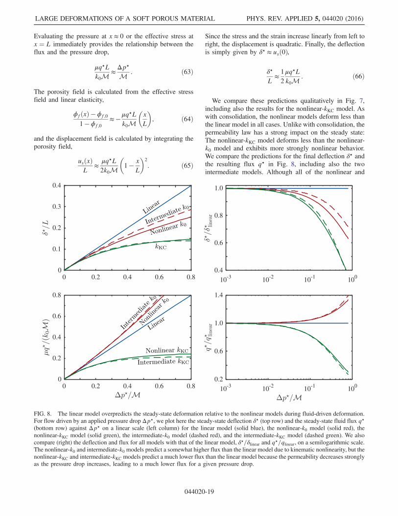
We compare these predictions qualitatively in Fig. 7,including also the results for the nonlinear-kKC model. Aswith consolidation, the nonlinear models deform less thanthe linear model in all cases. Unlike with consolidation, thepermeability law has a strong impact on the steady state:The nonlinear-kKC model deforms less than the nonlinear-k0 model and exhibits more strongly nonlinear behavior.We compare the predictions for the final deflection δ⋆ andthe resulting flux q⋆ in Fig. 8, including also the twointermediate models. Although all of the nonlinear and

FIG. 8. The linear model overpredicts the steady-state deformation relative to the nonlinear models during fluid-driven deformation.For flow driven by an applied pressure drop Δp⋆, we plot here the steady-state deflection δ⋆ (top row) and the steady-state fluid flux q⋆(bottom row) against Δp⋆ on a linear scale (left column) for the linear model (solid blue), the nonlinear-k0 model (solid red), thenonlinear-kKC model (solid green), the intermediate-k0 model (dashed red), and the intermediate-kKC model (dashed green). We alsocompare (right) the deflection and flux for all models with that of the linear model, δ⋆=δlinear and q⋆=qlinear, on a semilogarithmic scale.The nonlinear-k0 and intermediate-k0 models predict a somewhat higher flux than the linear model due to kinematic nonlinearity, but thenonlinear-kKC and intermediate-kKC models predict a much lower flux than the linear model because the permeability decreases stronglyas the pressure drop increases, leading to a much lower flux for a given pressure drop.


044020-19

intermediate models predict a much smaller deflectionthan the linear model, the nonlinear-k0 and intermediate-k0 models predict a larger steady-state flux than the linearmodel, whereas the nonlinear-kKC and intermediate-kKCmodels predict a much smaller steady-state flux. Thisoccurs because the steady-state flux results from twocompeting physical effects. As the driving pressure dropincreases, we expect the deflection to increase. As thedeflection increases, the overall length of the skeleton

decreases, and, since the pressure drop is fixed, the pressuregradient across the material increases. As a result, weexpect from Darcy’s law that the flux will scale likeq⋆ ∼ ðk=μÞΔp⋆=ðL − δ⋆Þ. For constant permeability, wethen expect the flux to increase faster than linearly withΔp⋆, and this is indeed what we see for the nonlinear-k0and intermediate-k0 cases. The changing length is akinematic nonlinearity that is neglected in the linear model,so q⋆linear is simply proportional to Δp⋆ despite the fact that

FIG. 9. Dynamics of fluid-driven deformation for a soft porous material, where the net flow from left to right is driven by an appliedpressure dropΔp⋆ ¼ 0.5.We show the porosity (first row), displacement (second row), effective stress (third row), and pressure (last row)at t=Tpe ¼ 0, 0.001, 0.003, 0.01, 0.03, 0.1, and 0.3, as indicated (light to dark colors), for the linear model (left column, blue), thenonlinear-k0 model (middle column, red), and the nonlinear-kKC model (right column, green). For the nonlinear models, we plot theseresults against the Lagrangian coordinateX ¼ x − usðx; tÞ for clarity; for the linear model, we again adopt a Lagrangian interpretation andsimply replace x with X in the relevant expressions (see Secs. III C and V B). These results are for ϕf;0 ¼ 0.5.


044020-20

δ⋆linear is actually larger than the nonlinear or intermediatepredictions. However, these models ignore the fact that theporosity decreases as the deformation increases. When thepermeability is deformation dependent, this decreases verystrongly with the porosity and overwhelms the effect of thechanging length, leading to a strongly slower-than-lineargrowth of q⋆ with Δp⋆, and this is indeed what we see forthe nonlinear-kKC and intermediate-kKC models.

1. Dynamics

We next focus on the dynamic evolution of the defor-mation. We again solve the nonlinear and intermediatemodels numerically (Appendix C and Ref. [79]), and weagain solve the linear model analytically via separation ofvariables. The analytical solution can be written

ϕfðx; tÞ ¼ ϕf;0 þ ðϕ⋆f − ϕf;0Þ

�xLþX∞n¼1

2

nπ½ð−1Þn�e−½ðnπÞ2tÞ=Tpe� sin

�nπxL

��; ð67aÞ

usðx; tÞL

¼ −�ϕ⋆f − ϕf;0

1 − ϕf;0

��1

2

�1 −

�xL

�2�−X∞

n¼1

2

ðnπÞ2 ½ð−1Þn�e−f½ðnπÞ2t�=Tpeg

�ð−1Þn − cos

�nπxL

��; ð67bÞ

where ϕfð0; tÞ ¼ ϕf;0 and ϕfðL; tÞ ¼ ϕ⋆f ¼ ϕf;0 −

ð1 − ϕf;0ÞðΔp⋆=MÞ. We compare these solutions qualita-tively in Fig. 9, including also the results for the nonlinear-kKC case. Note once again that the spatial coordinate in thelinear model is ambiguous, and we again adopt a Lagran-gian interpretation.When the flow starts, the fluid and the solid initially travel

together to the right. The pressure remains uniform through-out most of the skeleton since there is no net flux of fluidthrough the skeleton, but there is a very sharp pressuregradient at the right edge where the solid is necessarilystationary. The motion of the solid toward the right boundarygradually compresses the right edge of the skeleton against

the boundary, and this motion slows over time as theeffective stress builds from right to left. The motion ofthe solid eventually stops, and the deformation reaches thesteady state when the strain in the skeleton is such that thegradient in effective stress balances the gradient in pressure.In this steady state, the skeleton remains completely relaxedat the left edge and is the most compressed at the right edge.From left to right, there is a gradual increase in deformationand magnitude of effective stress, and a gradual decrease inpressure and porosity.Both here and in the consolidation problem, the defor-

mation evolves with a classic boundary-layer structure thatmay be susceptible to a matched asymptotic approach with

FIG. 10. Relaxation toward the steady state during fluid-driven deformation with Δp⋆=M ¼ 0.5 on a linear scale (left) and on asemilogarithmic scale (right). We plot the relative difference between δðtÞ and its final value δ⋆ as a proxy for the global approach to thesteady state. We show again the linear (blue), nonlinear-k0 (red), and nonlinear-kKC (green) models. The final deflection δ⋆ is largest forthe linear model, followed by the nonlinear-k0 model, followed by the nonlinear-kKC model (δ⋆ ¼ 0.25, 0.181, and 0.127, respectively;cf. Fig. 8). As with consolidation, however, the nonlinear-k0 model relaxes more quickly than the linear model (at more than twice therate), whereas the nonlinear-kKC model relaxes more slowly than the linear model (at about 80% of the rate; cf. Fig. 5). These results arefor ϕf;0 ¼ 0.5.


044020-21

t=Tpe the small parameter. The prospect of more accuratelycapturing the kinematic nonlinearity while retaining somedegree of analytical tractability is a promising one forfuture work.To examine the time scale of the deformation, we plot the

evolution of the deflection toward its final value as a proxyfor the global approach to the steady state (Fig. 10). As forconsolidation, we find that the deflection approaches thesteady state exponentially in all cases, and that the non-linear-k0 and nonlinear-kKC models evolve more quicklyand more slowly than the linear model, respectively. Wealso investigate the impact of Δp⋆ on the time scale(Fig. 11). We find that the general trend is the same asin consolidation (cf. Fig. 6) but that the magnitude of theeffect is smaller—that is, the time scale during fluid-drivendeformation depends less strongly on Δp⋆ than the timescale during consolidation depends on σ0⋆. This is mostlikely due to the fact that the steady state is uniform inconsolidation, with potentially large compression through-out the entire material, whereas the steady state in fluid-driven deformation is highly nonuniform, with completelyrelaxed material at the left and highly compressed materialat the right.

VII. DISCUSSION AND CONCLUSIONS

We have provided an overview and discussion of acomplete Eulerian framework for the arbitrarily largedeformation of a porous material. In doing so, our maingoals were to (a) elucidate the key aspects of the rigorousmodel, (b) provide physical insight into the subtleties ofporomechanical coupling, and (c) investigate the

qualitative and quantitative nature of the error introducedby linearizing this model. These points are often obscuredby the powerful mathematical and computational machi-nery that is typically brought to bear on these problems.We intend that our approach here can serve as a concise,coherent, and approachable introduction to a large body ofwork in classical continuum and poromechanics. Webelieve that this overview now provides a rostrum tofacilitate further theoretical advances and new applicationsin soil mechanics, hydrogeology, biophysics, and bio-medical engineering.We have also applied this theory to two canonical model

problems in uniaxial deformation, one in which deforma-tion drives fluid flow and one in which fluid flow drivesdeformation. In the former, the consolidation problem, anapplied effective stress squeezes fluid from a porousmaterial. Although the steady state is simple and controlledentirely by the solid mechanics, the evolution of thedeformation is controlled by the rate at which fluid canflow through the material and out at the boundaries; weshowed that the resulting rate of relaxation is impactedstrongly by kinematic nonlinearity and even more stronglyby deformation-dependent permeability. In the latter prob-lem, fluid-driven deformation, a net throughflow com-presses the material against a rigid permeable boundary.The steady state is highly nonuniform, controlled by thesteady balance between the gradient in pressure and thegradient in stress. We showed that both the evolution of thedeformation and the deflection and fluid flux at the steadystate are impacted strongly by kinematic nonlinearity and,again, even more strongly by deformation-dependentpermeability.

FIG. 11. The deformation approaches the steady state more quickly for larger Δp⋆ when the permeability is constant and more slowlyfor larger Δp⋆ when the permeability is deformation dependent. Here, we plot (left) the relaxation time scale τ=Tpe against Δp⋆ for thelinear (solid blue), nonlinear-k0 (solid red), nonlinear-kKC (solid green), intermediate-k0 (dashed red), and intermediate-kKC (dashedgreen) models. The time scale is constant and equal to π−2 for the linear model but increases with Δp⋆ for the two k0 models anddecreases with Δp⋆ for the two kKC models. We also compare the relaxation time scales of all models with that of the linear model byplotting (right) τ=τlinear on a semilogarithmic scale. These results are for ϕf;0 ¼ 0.5.


044020-22

In the interest of emphasizing the nonlinear kinematicsof large deformations, we have avoided complex, material-specific constitutive models. Hencky elasticity captures thefull kinematic nonlinearity of large deformations in a verysimple form, and we believe that it provides a reasonablecompromise between rigor and complexity for moderatedeformations. However, real materials will always behavein a complex, material-specific way when subject tosufficiently large strains, and the framework consideredhere is fully compatible with other constitutive models.Similarly, we have considered one specific case of defor-mation-dependent permeability: the normalized Kozeny-Carman formula. We have shown that this typicallyamplifies the importance of kinematic nonlinearity andhas striking qualitative and quantitative impacts on poro-mechanical behavior. Although this example captures thekey qualitative features of the coupling between deforma-tion and permeability, material-specific relationships willbe needed to provide quantitative predictions for realmaterials.In describing the kinematics of the solid skeleton, we

have adopted the single assumption that the constituentmaterial is incompressible. This has clear relevance to soilmechanics, biophysics, and any other situation where thepressure and stress are small compared to the bulk modulusof the solid grains (e.g., approximately 30–40 GPa forquartz sand). This assumption can be relaxed, althoughdoing so substantially complicates the large-deformationtheory (e.g., Refs. [32,50,52]). We have also focused on thecase of a single, incompressible pore fluid, but the theory isreadily generalized to a compressible or multiphase fluidsystem (e.g., Refs. [32,43]).Uniaxial deformations have provided a convenient test

bed for our purposes here, but they are unusual in severalrespects that do not readily generalize to multiaxialscenarios. First, a uniaxial deformation can be fullycharacterized by the change in porosity, σ0xx ¼ σ0xxðϕfÞ;this simplifies the analysis, but it is not the case for evensimple biaxial deformations. Second, the cross sectionnormal to the flow does not deform or rotate, which greatlysimplifies the nonlinearity of poromechanical coupling.Finally, the exact relationship between displacement andporosity is linear; this is again not the case for even simplebiaxial deformations. We expect kinematic nonlinearity toplay an even stronger role for multiaxial deformations.

ACKNOWLEDGMENTS

The authors gratefully acknowledge support from theYale Climate & Energy Institute. E. R. D. acknowledgessupport from the National Science Foundation (GrantNo. CBET-1236086). J. S. W. acknowledges support fromYale University, the Swedish Research Council(Vetenskapsrådet Grant No. 638-2013-9243), and aRoyal Society Wolfson Research Merit Award.

APPENDIX A: LARGE-DEFORMATIONPOROELASTICITY IN A LAGRANGIAN

FRAMEWORK

Here we briefly summarize the Lagrangian approach tolarge-deformation poroelasticity, a thorough discussion andderivation of which is provided by Coussy [32]. In aLagrangian frame, it is natural to work with so-callednominal quantities, which measure the current stresses,fluxes, etc., acting on or through the reference areas orvolumes. For example, the nominal porosity Φf measuresthe current fluid volume per unit reference total volume andis related to the true porosity via Φf ¼ Jϕf. We denote thegradient and divergence operators in the Lagrangiancoordinate system by gradð·Þ and divð·Þ, respectively, todistinguish them from the corresponding operators in theEulerian coordinate system. The Lagrangian displacementfield is

Us ¼ xðX; tÞ −X; ðA1Þ

where X is the Lagrangian (material) coordinate, andxðX; tÞ is the current position of the skeleton that isinitially at position X. The corresponding deformation-gradient tensor is

F ¼ gradðxÞ ¼ Iþ gradðUsÞ: ðA2Þ

The Jacobian determinant is then related to Φf by

J ¼ detðFÞ ¼ 1þ Φf − Φf;0; ðA3Þ

where Φf;0ðXÞ is the reference porosity field, which weagain take to be undeformed. Continuity requires that

∂Φf

∂t þ divðWfÞ ¼ 0; ðA4Þ

where Wf is the nominal flux of fluid through the solidskeleton. The nominal flux is related to the pressuregradient via Darcy’s law,

Wf ¼ −JF−1F−T ·kðϕfÞμ

gradðpÞ; ðA5Þ

where the JF−1 portion of the prefactor converts the trueflux to the nominal flux, and the remaining factor of F−Tconverts the Eulerian gradient to the Lagrangian one.Mechanical equilibrium requires that

divðsÞ ¼ 0; ðA6Þ

where s is the nominal total stress, which is related to thetrue total stress via


044020-23

s ¼ JσF−T: ðA7Þ

The nominal effective stress s0 is then given by

s0 ¼ sþ JF−Tp: ðA8Þ

Combining Eqs. (A4)–(A8), we finally have

∂Φf

∂t − div

�JF−1F−T ·

kðϕfÞμ

gradðpÞ�¼ 0 and ðA9aÞ

divðs0Þ ¼ divðJF−TpÞ: ðA9bÞ

Supplemented with a constitutive law for the solid skeleton(relating s0 to Us) and appropriate boundary conditions,Eqs. (A9) constitute a complete formulation of poroelas-ticity in a Lagrangian framework [32]. The Lagrangianformulation is more suitable for computation than theEulerian formulation since the domain is fixed, but theunderlying physical structure is substantially more opaque.Note that the permeability must remain a function of thetrue porosity, k ¼ kðϕfÞ ¼ kðΦf=JÞ.Linearizing Eqs. (A9) in the strain and reverting from the

nominal porosity to the true porosity leads to

∂ϕf

∂t − div

�ð1 − ϕf;0Þ

k0μgradðpÞ

�≈ 0 and ðA10aÞ

divðσ0Þ ≈ gradðpÞ; ðA10bÞ

which coincide with Eqs. (24) and (19), respectively, butreplacing x with X. Note that the nominal porosity and thetrue porosity differ at leading order:

Φf − Φf;0 ¼ϕf − ϕf;0

1 − ϕf≈ϕf − ϕf;0

1 − ϕf;0; ðA11Þ

where the reference fields are always precisely equivalentΦf;0 ≡ ϕf;0, because they must necessarily refer to thesame reference state.

APPENDIX B: EULERIAN AND LAGRANGIANINTERPRETATIONS OF LINEAR ELASTICITY

The Eulerian (Eulerian-Almansi) and Lagrangian(Green-Lagrange) finite-strain tensors are

e ¼ 1

2ðI −B−1Þ ¼ 1

2ðI − F−TF−1Þ ðB1Þ

and

E ¼ 1

2ðC − IÞ ¼ 1

2ðFTF − IÞ; ðB2Þ

respectively. Linear elasticity, as described above, is effec-tively a linearized Eulerian constitutive law, where stress is

linear in the Eulerian infinitesimal strain

εe ¼1

2

�∂us

∂x þ�∂us

∂x�

T�¼ I − 1

2ðF−1 þ F−TÞ: ðB3Þ

However, it is equally valid to write a linearized Lagrangianconstitutive law, where stress is linear in the Lagrangianinfinitesimal strain

εE ¼ 1

2

�∂us

∂X þ�∂us

∂X�

T�¼ 1

2ðFþ FTÞ − I: ðB4Þ

The former quantity is nonlinear in a Lagrangian frame,whereas the latter quantity is nonlinear in an Eulerianframe. We use the linearized Eulerian law above, but in aLagrangian frame it will be more appropriate to use thelinearized Lagrangian law. The results are equivalent atleading order in the strain (∂u=∂x ≈ ∂u=∂X), but theydiverge as strains become non-negligible.

APPENDIX C: FINITE-VOLUME METHODWITH A MOVING BOUNDARY

To solve Eq. (31a) numerically, we formulate a finite-volume method on an adaptive grid. We provide a referenceimplementation in the Supplemental Material [79]. At anytime t, thedomainextends fromx ¼ δðtÞ tox ¼ L.Wedividethis domain into N cells of equal width ΔxðtÞ ¼½L − δðtÞ�=N, where cell i has center xiðtÞ ¼ δðtÞ þði − 1=2ÞΔxðtÞ, and we denote its left and right edges byxi−1=2ðtÞ¼xiðtÞ−ΔxðtÞ=2 and xiþ1=2ðtÞ¼xiðtÞþΔxðtÞ=2,respectively. Making use of the expressions

∂∂tΔx ¼ − 1

Ndδdt

¼ − ΔxL − δ

_δ and ðC1aÞ

∂∂t xi ¼

L − xiL − δ

_δ; ðC1bÞ

we formulate a finite-volume method in the standard way(e.g., Ref. [87]) by integrating Eq. (31a) over cell i,

Zxiþ1=2

xi−1=2

�∂ϕf

∂t þ ∂∂x ½ϕfvf�

�dx ¼ 0; ðC2Þ

where

ϕfvf ¼ ϕfqðtÞ − ð1 − ϕfÞkðϕfÞμ

∂p∂x ; ðC3Þ

as derived above. We arrive atZ

xiþ1=2

xi−1=2

∂ϕf

∂t dxþ ½ϕfvf��xiþ1=2

xi−1=2¼ 0: ðC4Þ

After manipulating the first term using the Leibniz integralrule and regrouping, we have


044020-24

∂∂t

Zxiþ1=2

xi−1=2ϕfdxþ

�−�L − xL − δ

�ϕf

_δþ ϕfvf

��xiþ1=2

xi−1=2¼ 0:

ðC5Þ

Defining ϕf;i to be the average of ϕf within cell i,

ϕf;i ≡ 1

Δx

Zxiþ1=2

xi−1=2ϕfdx; ðC6Þ

we finally have

∂ϕf;i

∂t −�

_δ

L − δ

�ϕf;i þ

1

Δx

�−�L − xL − δ

�ϕf

_δþ ϕfvf

��xiþ1=2

xi−1=2

¼ 0: ðC7Þ

We discretize the quantity in square brackets using upwind-ing for the advective components and central differencingfor the diffusive components. Simultaneously, we must alsosolve an evolution equation for the position of the movingboundary. This comes from Eqs. (31c) and (35),

_δ ¼ qðtÞ þ�kðϕfÞμ

∂p∂x

��x¼δ

: ðC8Þ

This system can be written directly in terms of the porosityonce a stress-strain constitutive law is specified, at whichpoint we have a closed set of equations in ϕf and δ. Weintegrate these equations in time using an explicit Runge-Kutta scheme.

APPENDIX D: STEADY-STATE SOLUTIONS:GENERAL PROCEDURE

At steady state, it is possible to construct (usuallyimplicit) analytical solutions for any combination ofelasticity and permeability law. We outline the generalprocedure below and provide a reference implementation inthe Supplemental Material [79]. Barry and Aldis [88]suggest a somewhat similar procedure for axisymmetricgeometries (cf. Ref. [88], Sec. V).Of the four quantities σ0⋆, q⋆, Δp⋆, and δ⋆, two must be

known in advance. We assume here that these are σ0⋆ andeither q⋆ or Δp⋆, but it is straightforward to adapt or invertthis procedure for other pairs. This procedure degenerateswhen there is no flow at steady state, q⋆¼0↔Δp⋆¼0, asin consolidation. The solution then depends only on thesolid mechanics and is very straightforward to derivedirectly from the mechanics of uniaxial strain.(1) We begin by formulating, and evaluating if possible,

two dimensionless indefinite integrals:

I1ðϕfÞ≡ 1

k0M

ZkðϕfÞ

dσ0xxdϕf

dϕf and ðD1aÞ

I2ðϕfÞ≡ 1

k0M

Z �ϕf − ϕf;0

1 − ϕf;0

�kðϕfÞ

dσ0xxdϕf

dϕf:

ðD1bÞThis relies on the fact that the effective stress canalways be written directly in terms of the porosity inthis geometry, σ0xx ¼ σ0xxðϕfÞ (see the discussion atthe end of Sec. IV B 2). For the elasticity andpermeability laws considered above, we providethe results in Appendix F.

(2) At steady state, we have that vs ¼ 0 and ϕfvf ¼ q⋆.The former statement with Eq. (31c) or the latterstatement with Eq. (31b) leads to

q⋆ þ kðϕfÞμ

∂σ0xx∂x ¼ 0; ðD2Þ

where we replace the pressure gradient with theeffective stress gradientusingEq. (31d).Equation (D2)can be rearranged and integrated to give

− μq⋆Lk0M

�xL− δ⋆

L

�¼ I1ðϕfðxÞÞ − I1ðϕfðδ⋆ÞÞ;

ðD3Þ

where ϕfðδ⋆Þ is calculated from σ0⋆ by invertingσ0xxðϕfðδ⋆ÞÞ ¼ σ0⋆. We next derive an expressionfor usðxÞ using Eq. (30), which can be rearrangedusing Eq. (D2) and then integrated to give

usðxÞL

¼ δ⋆L− k0Mμq⋆L ½I2ðϕfðxÞÞ − I2ðϕfðδ⋆ÞÞ�;

ðD4Þ

where we apply the boundary condition thatusðδ⋆Þ ¼ δ⋆. Finally, we evaluate Eqs. (D3) and(D4) at x ¼ L by applying the boundary conditionthat usðLÞ ¼ 0 and rearranging to eliminate δ⋆:

½I2ðϕfðLÞÞ − I2ðϕfðδ⋆ÞÞ�

− ½I1ðϕfðLÞÞ − I1ðϕfðδ⋆ÞÞ� ¼μq⋆Lk0M

: ðD5Þ

If Δp⋆ is known, ϕfðLÞ can calculated by invertingσ0xxðϕfðLÞÞ ¼ σ0⋆ − Δp⋆. Equation (D5) then pro-vides an explicit expression for q⋆. If q⋆ is knowninstead, Eq. (D5) provides an implicit expression forϕfðLÞ, which can then be used to calculate Δp⋆from Δp⋆ ¼ σ0⋆ − σ0xxðϕfðLÞÞ.

(3) Now that both q⋆ and Δp⋆ are known, δ⋆ can becalculated explicitly from Eq. (D4) evaluated atx ¼ L,


044020-25

δ⋆L

¼ k0Mμq⋆L ½I2ðϕfðLÞÞ − I2ðϕfðδ⋆ÞÞ�: ðD6Þ

(4) Equation (D3) now provides an implicit expressionfor ϕfðxÞ in terms of q⋆ and δ⋆.

(5) Equation (D4) now provides an explicit expressionfor usðxÞ in terms of q⋆, δ⋆, and ϕfðxÞ.

(6) Finally, the effective stress can be calculated fromϕfðxÞ and then the pressure from the effective stress,

σ0xxðxÞ ¼ σ0xxðϕfðxÞÞ; ðD7aÞ

pðxÞ ¼ σ0xxðxÞ − ðσ0⋆ − Δp⋆Þ; ðD7bÞ

where the latter comes from integrating Eq. (31d) andapplying the final boundary condition, pðLÞ ¼ 0.

This procedure can be implemented analytically as longas the integrals can be evaluated exactly, although numeri-cal root finding is required in most cases. When theintegrals cannot be evaluated exactly, it is straightforwardto implement them numerically using standard quadraturetechniques.

APPENDIX E: STEADY-STATE SOLUTIONS:MAXIMUM VALUES

The effective stress is always largest in magnitude at theright boundary (x ¼ L), so this is where the porosity andpermeability are the smallest, and the flow must stop whenthese vanish. Provided that σ0⋆ is known, this conditionallows for the direct calculation of the maximum achievablevalues q⋆max, Δp⋆

max, and δ⋆max for which the porosityvanishes at x ¼ L. The maximum flux q⋆max can beevaluated directly from Eq. (D5) by setting ϕfðLÞ ¼ 0,

μq⋆maxLk0M

¼ ½I2ð0Þ − I2ðϕfðδ⋆ÞÞ�

− ½I1ð0Þ − I1ðϕfðδ⋆ÞÞ�: ðE1Þ

The maximum pressure drop Δp⋆max can be evaluated

directly from the elasticity law by setting ϕfðLÞ ¼ 0,

Δp⋆max ¼ σ0⋆ − σ0xxðϕf ¼ 0Þ: ðE2Þ

The maximum deflection δ⋆max can be evaluated directlyfrom Eq. (D6) by setting q⋆ ¼ q⋆max and ϕfðLÞ ¼ 0,

δ⋆max

L¼ k0M

μq⋆maxL½I2ð0Þ − I2ðϕfðδ⋆ÞÞ�: ðE3Þ

These three values occur simultaneously for a given σ0⋆,and they are physical limits in the sense that it is notpossible to drive a flux greater than q⋆max or a deflectiongreater than δ⋆max, or to apply a pressure drop greater thanΔp⋆

max, without producing a negative porosity at the rightboundary. Although solutions may exist for larger values,they will be nonphysical.

APPENDIX F: STEADY-STATE SOLUTIONS:INTEGRALS FOR SPECIFIC CASES

Here, we evaluate the integrals I1ðϕfÞ and I2ðϕfÞ[Eq. (D1)] for the scenarios considered in Sec. VI A: linearelasticity (for use with the intermediate model) and Henckyelasticity (for use with the nonlinear model), each for bothconstant permeability (k¼k0) and deformation-dependentpermeability [k¼kðϕfÞ via the normalized Kozeny-Carmanformula,Eq. (12)]. Ineachcase,we firstwrite theelasticity lawin terms of the porosity and then evaluate the first derivative ofthis function. For linear elasticity, we have

σ0xxðϕfÞM

¼ ϕf − ϕf;0

1 − ϕf;0and

1

Mdσ0xxdϕf

¼ 1

1 − ϕf;0: ðF1Þ

For Hencky elasticity, we instead have

σ0xxðϕfÞM

¼�1 − ϕf

1 − ϕf;0

�ln

�1 − ϕf;0

1 − ϕf

�and ðF2aÞ

1

Mdσ0xxdϕf

¼ 1

1 − ϕf;0

�1 − ln

�1 − ϕf;0

1 − ϕf

��: ðF2bÞ

We now evaluate the two integrals. These expressions can then be used with the procedure described in Appendix D toevaluate the full steady-state solutions for these constitutive models. Note that the integrals are indefinite, so arbitraryconstants can be added or subtracted from the expressions below without loss of generality.


044020-26

(i) Intermediate k0 (linear elasticity with constant permeability)

I1ðϕfÞ ¼ϕf − ϕf;0

1 − ϕf;0and I2ðϕfÞ ¼

1

2

�ϕf − ϕf;0

1 − ϕf;0

�2

: ðF3Þ

(ii) Intermediate kKC (linear elasticity with normalized Kozeny-Carman permeability)

I1ðϕfÞ ¼1 − ϕf;0

ϕ3f;0

�1

2ϕ2f þ 2ϕf þ

1

1 − ϕfþ 3 lnð1 − ϕfÞ

�and ðF4aÞ

I2ðϕfÞ ¼1

ϕ3f;0

�− 1

3ð1 − ϕfÞ3 þ

1

2ð4 − ϕf;0Þð1 − ϕfÞ2 − 3ð2 − ϕf;0Þð1 − ϕfÞ

þ 1 − ϕf;0

1 − ϕfþ ð4 − 3ϕf;0Þ lnð1 − ϕfÞ

�: ðF4bÞ

(iii) Nonlinear k0 (Hencky elasticity with constant permeability)

I1ðϕfÞ ¼�1 − ϕf

1 − ϕf;0

�ln

�1 − ϕf;0

1 − ϕf

�and ðF5aÞ

I2ðϕfÞ ¼1

4

�1 − ϕf

1 − ϕf;0

�2

þ 1

2

�1 −

�ϕf − ϕf;0

1 − ϕf;0

�2�ln

�1 − ϕf;0

1 − ϕf

�: ðF5bÞ

(IV) Nonlinear kKC (Hencky elasticity with normalized Kozeny-Carman permeability)

I1ðϕfÞ ¼1 − ϕf;0

4ϕ3f;0

�ϕ2f þ 2

�ϕ3f þ 3ϕ2

f − 4ϕf − 2

1 − ϕf

�ln

�1 − ϕf;0

1 − ϕf

�

þ 6ln2�1 − ϕf;0

1 − ϕf

�− 2ϕf þ

8

1 − ϕfþ 2 lnð1 − ϕfÞ

�; ðF6aÞ

I2ðϕfÞ ¼1

36ϕ3f;0

�8ϕ3

f þ 3ð4 − 3ϕf;0Þϕ2f − 6ð8 − 3ϕf;0Þϕf − 6ð2þ 3ϕf;0Þ lnð1 − ϕfÞ

þ 6

�2ϕ4

f þ ð4 − 3ϕf;0Þð3þ ϕfÞϕ2f − 6ð3 − 2ϕf;0Þϕf − 6ð1 − ϕf;0Þ1 − ϕf

�ln

�1 − ϕf;0

1 − ϕf

�

þ 72

�1 − ϕf;0

1 − ϕf

�þ 18ð4 − 3ϕf;0Þln2

�1 − ϕf;0

1 − ϕf

��: ðF6bÞ

[1] V. C. Mow, S. C. Kuei, W.M. Lai, and C. G. Armstrong,Biphasic creep and stress relaxation of articular cartilage incompression: Theory and experiments, J. Biomech. Eng.102, 73 (1980).

[2] W.M. Lai, J. S. Hou, and V. C. Mow, A triphasic theory forthe swelling and deformation behaviors of articular carti-lage, J. Biomech. Eng. 113, 245 (1991).

[3] M. Yang and L. A. Taber, The possible role of poroelasticityin the apparent viscoelastic behavior of passive cardiacmuscle, J. Biomech. 24, 587 (1991).

[4] S. C. Cowin, Bone poroelasticity, J. Biomech. 32, 217 (1999).

[5] G. Franceschini, D. Bigoni, P. Regitnig, and G. A.Holzapfel, Brain tissue deforms similarly to filledelastomers and follows consolidation theory, J. Mech. Phys.Solids 54, 2592 (2006).

[6] J. M. Skotheim and L. Mahadevan, Physical limits anddesign principles for plant and fungal movements, Science308, 1308 (2005).

[7] G. T. Charras, J. C. Yarrow, M. A. Horton, L. Mahadevan,and T. J. Mitchison, Non-equilibration of hydrostaticpressure in blebbing cells, Nature (London) 435, 365(2005).


044020-27

http://dx.doi.org/10.1115/1.3138202

http://dx.doi.org/10.1115/1.3138202

http://dx.doi.org/10.1115/1.2894880

http://dx.doi.org/10.1016/0021-9290(91)90291-T

http://dx.doi.org/10.1016/S0021-9290(98)00161-4

http://dx.doi.org/10.1016/j.jmps.2006.05.004


http://dx.doi.org/10.1126/science.1107976

http://dx.doi.org/10.1126/science.1107976

http://dx.doi.org/10.1038/nature03550

http://dx.doi.org/10.1038/nature03550

[8] J. Dumais and Y. Forterre, Vegetable dynamicks: The role ofwater in plant movements, Annu. Rev. Fluid Mech. 44, 453(2012).

[9] E. Moeendarbary, L. Valon, M. Fritzsche, A. R. Harris,D. A. Moulding, A. J. Thrasher, E. Stride, L. Mahadevan,and G. T. Charras, The cytoplasm of living cells behaves as aporoelastic material, Nat. Mater. 12, 253 (2013).

[10] D. McKenzie, The generation and compaction of partiallymolten rock, J. Petrol. 25, 713 (1984).

[11] A. C.Fowler,Amathematicalmodel ofmagma transport in theasthenosphere,Geophys.Astrophys.FluidDyn.33, 63 (1985).

[12] M. Spiegelman, Flow in deformable porous media. Part 1.Simple analysis, J. Fluid Mech. 247, 17 (1993).

[13] D. Bercovici, Y. Ricard, and G. Schubert, A two-phasemodel for compaction and damage 1. General theory,J. Geophys. Res. 106, 8887 (2001).

[14] R. F. Katz, Magma dynamics with the enthalpy method:Benchmark solutions and magmatic focusing at mid-oceanridges, J. Petrol. 49, 2099 (2008).

[15] M. A. Hesse, A. R. Schiemenz, Y. Liang, and E. M.Parmentier, Compaction-dissolution waves in an upwellingmantle column, Geophys. J. Int. 187, 1057 (2011).

[16] J. Bear and M. Y. Corapcioglu, Mathematical model forregional land subsidence due to pumping: 1. Integratedaquifer subsidence equations based on vertical displacementonly, Water Resour. Res. 17, 937 (1981).

[17] H. F. Wang, Theory of Linear Poroelasticity (PrincetonUniversity Press, Princeton, NJ, 2000).

[18] M. L. Szulczewski, C. W. MacMinn, H. J. Herzog, and R.Juanes, Lifetime of carbon capture and storage as a climate-change mitigation technology, Proc. Natl. Acad. Sci. U.S.A.109, 5185 (2012).

[19] J. Rutqvist, The geomechanics of CO2 storage in deepsedimentary formations, Geotechnical and geologicalengineering 30, 525 (2012).

[20] K.W. Chang, M. A. Hesse, and J.-P. Nicot, Reduction inlateral pressure propagation due to dissipation into ambientmudrocks during geological carbon dioxide storage, WaterResour. Res. 49, 2573 (2013).

[21] J. P. Verdon, J.-M. Kendall, A. L. Stork, R. A. Chadwick,D. J. White, and R. C. Bissell, Comparison of geomechan-ical deformation induced by megatonne-scale CO2 storageat Sleipner, Weyburn, and In Salah, Proc. Natl. Acad. Sci.U.S.A. 110, E2762 (2013).

[22] V. M. Yarushina, D. Bercovici, and M. L. Oristaglio, Rockdeformation models and fluid leak-off in hydraulic fractur-ing, Geophys. J. Int. 194, 1514 (2013).

[23] B. Jha and R. Juanes, Coupled multiphase flow andporomechanics: A computational model of pore-pressureeffects on fault slip and earthquake triggering, WaterResour. Res. 50, 3776 (2014).

[24] Z. Cai and D. Bercovici, Two-phase viscoelastic damagetheory, with applications to subsurface fluid injection,Geophys. J. Int. 199, 1481 (2014).

[25] D. R. Hewitt, J. A. Neufeld, and N. J. Balmforth, Shallow,gravity-driven flow in a poro-elastic layer, J. Fluid Mech.778, 335 (2015).

[26] R. de Boer, Highlights in the historical development of theporous media theory: Toward a consistent macroscopictheory, Appl. Mech. Rev. 49, 201 (1996).

[27] M. A. Biot, General theory of three-dimensional consoli-dation, J. Appl. Phys. 12, 155 (1941).

[28] M. A. Biot, Theory of propagation of elastic waves in afluid-saturated porous solid. I. Low-frequency range,J. Acoust. Soc. Am. 28, 168 (1956).

[29] M. A. Biot, Mechanics of deformation and acoustic propa-gation in porous media, J. Appl. Phys. 33, 1482 (1962).

[30] J. R. Rice and M. P. Cleary, Some basic stress diffusionsolutions for fluid-saturated elastic porous media withcompressible constituents, Rev. Geophys. Space Phys. 14,227 (1976).

[31] M. A. Biot, Theory of finite deformations of porous solids,Indiana University Mathematics Journal 21, 597 (1972).

[32] O. Coussy, Poromechanics (Wiley, New York, 2004).[33] M. H. Holmes and V. C. Mow, The nonlinear characteristics

of soft gels and hydrated connective tissues in ultrafiltration,J. Biomech. 23, 1145 (1990).

[34] M. K. Kwan, W. M. Lai, and V. C. Mow, A finitedeformation theory for cartilage and other soft hydratedconnective tissues—I. Equilibrium results, J. Biomech. 23,145 (1990).

[35] B. R. Simon, Multiphase poroelastic finite elementmodels for soft tissue structures, Appl. Mech. Rev. 45,191 (1992).

[36] M Argoubi and A Shirazi-Adl, Poroelastic creep responseanalysis of a lumbar motion segment in compression,J. Biomech. 29, 1331 (1996).

[37] S. Federico and A. Grillo, Elasticity and permeability ofporous fibre-reinforced materials under large deformations,Mech. Mater. 44, 58 (2012).

[38] A. Tomic, A. Grillo, and S. Federico, Poroelastic materialsreinforced by statistically oriented fibers—numerical im-plementation and applications to articular cartilage, IMA J.Appl. Math. 79, 1027 (2014).

[39] A.-T. Vuong, L. Yoshihara, and W. A. Wall, A generalapproach for modeling interacting flow through porousmedia under finite deformations, Comput. Methods Appl.Mech. Eng. 283, 1240 (2015).

[40] J. P. Carter, J. R. Booker, and J. C. Small, The analysis offinite elasto-plastic consolidation, Int. J. Numer. Anal.Methods Geomech. 3, 107 (1979).

[41] R. I. Borja and E. Alarcón, A mathematical framework forfinite strain elastoplastic consolidation. Part 1: Balancelaws, variational formulation, and linearization, Comput.Methods Appl. Mech. Eng. 122, 145 (1995).

[42] C. Li, R. I. Borja, and R. A. Regueiro, Dynamics of porousmedia at finite strain, Comput. Methods Appl. Mech. Eng.193, 3837 (2004).

[43] R. Uzuoka and R. I. Borja, Dynamics of unsaturatedporoelastic solids at finite strain, Int. J. Numer. Anal.Methods Geomech. 36, 1535 (2011).

[44] L. S. Bennethum and J. H. Cushman, Multiscale, hybridmixture theory for swelling systems—I: Balance laws, Int. J.Eng. Sci. 34, 125 (1996).

[45] J. M. Huyghe and J. D. Janssen, Quadriphasic mechanics ofswelling incompressible porous media, Int. J. Eng. Sci. 35,793 (1997).

[46] W. Hong, X. Zhao, J. Zhou, and Z. Suo, A theory of coupleddiffusion and large deformation in polymeric gels, J. Mech.Phys. Solids 56, 1779 (2008).


044020-28

http://dx.doi.org/10.1146/annurev-fluid-120710-101200

http://dx.doi.org/10.1146/annurev-fluid-120710-101200

http://dx.doi.org/10.1038/nmat3517

http://dx.doi.org/10.1093/petrology/25.3.713

http://dx.doi.org/10.1080/03091928508245423

http://dx.doi.org/10.1017/S0022112093000369

http://dx.doi.org/10.1029/2000JB900430

http://dx.doi.org/10.1093/petrology/egn058

http://dx.doi.org/10.1111/j.1365-246X.2011.05177.x

http://dx.doi.org/10.1029/WR017i004p00937

http://dx.doi.org/10.1073/pnas.1115347109


http://dx.doi.org/10.1007/s10706-011-9491-0

http://dx.doi.org/10.1007/s10706-011-9491-0

http://dx.doi.org/10.1002/wrcr.20197

http://dx.doi.org/10.1002/wrcr.20197



http://dx.doi.org/10.1093/gji/ggt199

http://dx.doi.org/10.1002/2013WR015175

http://dx.doi.org/10.1002/2013WR015175

http://dx.doi.org/10.1093/gji/ggu344

http://dx.doi.org/10.1017/jfm.2015.361

http://dx.doi.org/10.1017/jfm.2015.361

http://dx.doi.org/10.1115/1.3101926

http://dx.doi.org/10.1063/1.1712886

http://dx.doi.org/10.1121/1.1908239

http://dx.doi.org/10.1063/1.1728759

http://dx.doi.org/10.1029/RG014i002p00227

http://dx.doi.org/10.1029/RG014i002p00227

http://dx.doi.org/10.1512/iumj.1972.21.21048

http://dx.doi.org/10.1016/0021-9290(90)90007-P

http://dx.doi.org/10.1016/0021-9290(90)90348-7

http://dx.doi.org/10.1016/0021-9290(90)90348-7

http://dx.doi.org/10.1115/1.3121397

http://dx.doi.org/10.1115/1.3121397

http://dx.doi.org/10.1016/0021-9290(96)00035-8

http://dx.doi.org/10.1016/j.mechmat.2011.07.010

http://dx.doi.org/10.1093/imamat/hxu039

http://dx.doi.org/10.1093/imamat/hxu039

http://dx.doi.org/10.1016/j.cma.2014.08.018


http://dx.doi.org/10.1002/nag.1610030202


http://dx.doi.org/10.1016/0045-7825(94)00720-8

http://dx.doi.org/10.1016/0045-7825(94)00720-8





http://dx.doi.org/10.1016/0020-7225(95)00089-5

http://dx.doi.org/10.1016/0020-7225(95)00089-5

http://dx.doi.org/10.1016/S0020-7225(96)00119-X

http://dx.doi.org/10.1016/S0020-7225(96)00119-X



[47] F. P. Duda, A. C. Souza, and E. Fried, A theory for speciesmigration in a finitely strained solid with application topolymer network swelling, J. Mech. Phys. Solids 58, 515(2010).

[48] S. A. Chester and L. Anand, A coupled theory of fluidpermeation and large deformations for elastomeric materi-als, J. Mech. Phys. Solids 58, 1879 (2010).

[49] S. M. Hassanizadeh and W. G. Gray, General conservationequations for multi-phase systems: 1. Averaging procedure,Adv. Water Resour. 2, 131 (1979).

[50] L. S. Bennethum, Compressibility moduli for porous ma-terials incorporating volume fraction, J. Eng. Mech. 132,1205 (2006).

[51] J. C. Jaeger, N. G. W. Cook, and R. Zimmerman, Funda-mentals of Rock Mechanics, 4th ed. (Wiley-Blackwell,New York, 2007), ISBN: 978-0-632-05759-7.

[52] A. Gajo, A general approach to isothermal hyperelasticmodelling of saturated porous media at finite strains withcompressible solid constituents, Proc. R. Soc. A 466, 3061(2010).

[53] J. E. Marsden and T. J. R. Hughes, Mathematical Founda-tions of Elasticity (Dover Publications, Inc., New York,1983), ISBN 0-486-67865-2.

[54] M. E. Gurtin, E. Fried, and L. Anand, The Mechanics andThermodynamics of Continua (Cambridge University Press,Cambridge, England, 2010).

[55] R. B. Bird, R. C. Armstrong, and O. Hassager, Dynamics ofPolymer Liquids, Volume 1: Fluid Mechanics (Wiley-Interscience, New York, 1987).

[56] R. B. Bird, C. F. Curtiss, R. C. Armstrong, and O. Hassager,Dynamics of Polymer Liquids, Volume 2: Kinetic Theory(Wiley-Interscience, New York, 1987).

[57] G. F. Pinder and W. G. Gray, Essentials of Multiphase Flowin Porous Media (Wiley-Interscience, Hoboken, NJ, USA,2008).

[58] Y.-S. Wu and K. Pruess, Flow of non-Newtonian fluids inporous media, in Advances in Porous MediaVol. 3, Chap. 2,edited by M. Y. Corapcioglu (Elsevier, New York, 1996),pp. 87–184.

[59] K. von Terzaghi, The shearing resistance of saturatedsoil and the angle between the planes of shear, in Proceed-ings of the International Conference on Soil Mechanics andFoundation Engineering, June 22–26, 1936, Vol. 1,pp. 54–56.

[60] A. Nur and J. D. Byerlee, An exact effective stress law forelastic deformation of rock with fluids, J. Geophys. Res. 76,6414 (1971).

[61] L. Anand, On H. Hencky’s approximate strain-energyfunction for moderate deformations, J. Appl. Mech. 46,78 (1979).

[62] H. Xiao and L. S. Chen, Hencky’s elasticity model andlinear stress-strain relations in isotropic finite hyperelastic-ity, Acta Mech. 157, 51 (2002).

[63] L. Anand, Moderate deformations in extension-torsion ofincompressible isotropic elastic materials, J. Mech. Phys.Solids 34, 293 (1986).

[64] Z. P. Bažant, Easy-to-compute tensors with symmetricinverse approximating Hencky finite strain and its rate,J. Eng. Mater. Technol. 120, 131 (1998).

[65] G. S. Beavers and D. D. Joseph, Boundary conditionsat a naturally permeable wall, J. Fluid Mech. 30, 197 (1967).

[66] U. Shavit, Special issue on “Transport phenomena at theinterface between fluid and porous domains”, Transp.Porous Media 78, 327 (2009).

[67] K. Mosthaf, K. Baber, B. Flemisch, R. Helmig, A. Leijnse,I. Rybak, and B. Wohlmuth, A coupling concept for two-phase compositional porous-medium and single-phasecompositional free flow, Water Resour. Res. 47, W10522(2011).

[68] S. I. Barry and G. K. Aldis, Comparison of models for flowinduced deformation of soft biological tissue, J. Biomech.23, 647 (1990).

[69] S. I. Barry and G. K. Aldis, Unsteady flow induced defor-mation of porous materials, Int. J. Nonlinear Mech. 26, 687(1991).

[70] L. Preziosi, D. D. Joseph, and G. S. Beavers, Infiltration ofinitially dry, deformable porous media, Int. J. MultiphaseFlow 22, 1205 (1996).

[71] M. H. Holmes, Finite deformation of soft tissue: Analysis ofa mixture model in uni-axial compression, J. Biomech. Eng.108, 372 (1986).

[72] M. A. Dawson, G. H. McKinley, and L. J. Gibson, Thedynamic compressive response of an open-cell foam im-pregnated with a Newtonian fluid, J. Appl. Mech. 75,041015 (2008).

[73] J. L. Sommer and A. Mortensen, Forced unidirectionalinfiltration of deformable porous media, J. Fluid Mech.311, 193 (1996).

[74] D. M. Anderson, Imbibition of a liquid droplet on adeformable porous substrate, Phys. Fluids 17, 087104(2005).

[75] J. I. Siddique, D. M. Anderson, and A. Bondarev, Capillaryrise of a liquid into a deformable porous material, Phys.Fluids 21, 013106 (2009).

[76] G. S. Beavers, A. Hajji, and E. M. Sparrow, Fluid flowthrough a class of highly-deformable porous media. Part I:Experiments with air, J. Fluids Eng. 103, 432 (1981).

[77] G. S. Beavers, K. Wittenberg, and E. M. Sparrow, Fluidflow through a class of highly-deformable porous media.Part II: Experiments with water, J. Fluids Eng. 103, 440(1981).

[78] K. H. Parker, R. V. Mehta, and C. G. Caro, Steady flow inporous, elastically deformable materials, J. Appl. Mech. 54,794 (1987).

[79] See the Supplemental Material at http://link.aps.org/supplemental/10.1103/PhysRevApplied.5.044020 for aMATLAB implementation of the models, solutions, andresults presented in Secs. IV–VI.

[80] G. S. Beavers, T. A. Wilson, and B. A. Masha, Flow througha deformable porous material, J. Appl. Mech. 42, 598(1975).

[81] A. Oloyede and N. D. Broom, Is classical consolidationtheory applicable to articular cartilage deformation?, Clini-cal biomechanics 6, 206 (1991).

[82] M. A. Murad, L. S. Bennethum, and J. H. Cushman, Amulti-scale theory of swelling porous media: I. Applicationto one-dimensional consolidation, Transp. Porous Media 19,93 (1995).


044020-29




http://dx.doi.org/10.1016/0309-1708(79)90025-3

http://dx.doi.org/10.1061/(ASCE)0733-9399(2006)132:11(1205)

http://dx.doi.org/10.1061/(ASCE)0733-9399(2006)132:11(1205)

http://dx.doi.org/10.1098/rspa.2010.0018

http://dx.doi.org/10.1098/rspa.2010.0018

http://dx.doi.org/10.1029/JB076i026p06414

http://dx.doi.org/10.1029/JB076i026p06414

http://dx.doi.org/10.1115/1.3424532

http://dx.doi.org/10.1115/1.3424532

http://dx.doi.org/10.1007/BF01182154

http://dx.doi.org/10.1016/0022-5096(86)90021-9

http://dx.doi.org/10.1016/0022-5096(86)90021-9

http://dx.doi.org/10.1115/1.2807001

http://dx.doi.org/10.1017/S0022112067001375

http://dx.doi.org/10.1007/s11242-009-9414-1

http://dx.doi.org/10.1007/s11242-009-9414-1

http://dx.doi.org/10.1029/2011WR010685

http://dx.doi.org/10.1029/2011WR010685

http://dx.doi.org/10.1016/0021-9290(90)90164-X

http://dx.doi.org/10.1016/0021-9290(90)90164-X

http://dx.doi.org/10.1016/0020-7462(91)90020-T

http://dx.doi.org/10.1016/0020-7462(91)90020-T

http://dx.doi.org/10.1016/0301-9322(96)00035-3

http://dx.doi.org/10.1016/0301-9322(96)00035-3

http://dx.doi.org/10.1115/1.3138633

http://dx.doi.org/10.1115/1.3138633

http://dx.doi.org/10.1115/1.2912940

http://dx.doi.org/10.1115/1.2912940

http://dx.doi.org/10.1017/S002211209600256X

http://dx.doi.org/10.1017/S002211209600256X

http://dx.doi.org/10.1063/1.2000247

http://dx.doi.org/10.1063/1.2000247

http://dx.doi.org/10.1063/1.3068194

http://dx.doi.org/10.1063/1.3068194

http://dx.doi.org/10.1115/1.3240807

http://dx.doi.org/10.1115/1.3240810

http://dx.doi.org/10.1115/1.3240810

http://dx.doi.org/10.1115/1.3173119

http://dx.doi.org/10.1115/1.3173119

http://link.aps.org/supplemental/10.1103/PhysRevApplied.5.044020







http://dx.doi.org/10.1115/1.3423648

http://dx.doi.org/10.1115/1.3423648

http://dx.doi.org/10.1016/0268-0033(91)90048-U

http://dx.doi.org/10.1016/0268-0033(91)90048-U

http://dx.doi.org/10.1007/BF00626661

http://dx.doi.org/10.1007/BF00626661

[83] R. Lancellotta and L. Preziosi, A general nonlinear math-ematical model for soil consolidation problems, Int. J. Eng.Sci. 35, 1045 (1997).

[84] Y. Lanir, S. Sauob, and P. Maretsky, Nonlinear finitedeformation response of open cell polyurethane spongeto fluid filtration, J. Appl. Mech. 57, 449 (1990).

[85] B. Sobac, M. Colombani, and Y. Forterre, On thedynamics of poroelastic foams (in French), Mec. Ind. 12,231 (2011).

[86] D. R. Hewitt, J. S. Nijjer, M. G. Worster, and J. A. Neufeld,Flow-induced compaction of a deformable porous medium,Phys. Rev. E 93, 023116 (2016).

[87] R. J. LeVeque, Finite-Volume Methods for HyperbolicProblems (Cambridge University Press, Cambridge,England, 2004).

[88] S. I. Barry and G. K. Aldis, Radial flow through deformableporous shells, J. Aust. Math. Soc. Series B, Appl. Math. 34,333 (1993).


044020-30

http://dx.doi.org/10.1016/S0020-7225(97)00024-4

http://dx.doi.org/10.1016/S0020-7225(97)00024-4

http://dx.doi.org/10.1115/1.2892010

http://dx.doi.org/10.1051/meca/2011115

http://dx.doi.org/10.1051/meca/2011115

http://dx.doi.org/10.1103/PhysRevE.93.023116

http://dx.doi.org/10.1017/S0334270000008936

http://dx.doi.org/10.1017/S0334270000008936

large deformations of a soft porous material

Documents