analysis of deformations in soft clay due to...
TRANSCRIPT
Analysis of deformations in soft clay due to
unloading
Master of Science Thesis in the Master’s Programme Geo and Water Engineering
ARAZ ISMAIL
FITSUM TESHOME
Department of Civil and Environmental Engineering
Division of GeoEngineering
Geotechnical Engineering Research Group
CHALMERS UNIVERSITY OF TECHNOLOGY
Goteborg, Sweden 2011
Master’s Thesis 2011:23

MASTER’S THESIS 2011:23
Analysis of deformations in soft clay due to unloading
Master of Science Thesis in the Master’s Programme Geo and Water Engineering
ARAZ ISMAIL
FITSUM TESHOME
Department of Civil and Environmental Engineering
Division of GeoEngineering
Geotechnical Engineering Research Group
CHALMERS UNIVERSITY OF TECHNOLOGY
Göteborg, Sweden 2011
Analysis of deformations in soft clay due to unloading
Master of Science Thesis in the Master’s Programme Geo and Water Engineering
ARAZ ISMAIL
FITSUM TESHOME
© ARAZ ISMAIL & FITSUM TESHOME, 2011
Examensarbete / Institutionen för bygg- och miljöteknik,
Chalmers tekniska högskola 2011:23
Department of Civil and Environmental Engineering
Division of GeoEngineering
Geotechnical Engineering Research Group
Chalmers University of Technology
SE-412 96 Göteborg
Sweden
Telephone: + 46 (0)31-772 1000
Cover: Excavation under the bridge at section E13 at Lärjeholm and horizontal
displacement readings in contour form in Plaxis. The picture was taken by Fitsum
Teshome in January 2011.
Chalmers Reproservice
Göteborg, Sweden 2011
I
Analysis of deformations in soft clay due to unloading
Master of Science Thesis in the Master’s Programme Geo and Water Engineering
ARAZ ISMAIL
FITSUM TESHOME
Department of Civil and Environmental Engineering
Division of GeoEngineering
Geotechnical Engineering Research Group
Chalmers University of Technology
ABSTRACT
In infrastructure projects such as road and railway construction it is necessary to
perform a number of earth excavations wherever required. These excavations cause
difficulties regarding deformations and slope stability on the soil mass. The
deformation of soil is highly dependent on the stiffness of the soil. Therefore, it is of
particular interest to determine the appropriate stiffness modulus of soil in order to
study the deformation properties of soil. The objective of this thesis is to study in
depth the deformation of soft clay due to unloading or excavation.
In this project the excavation was carried out on section E13 at Lärjeholm which is
part of the undergoing new railway project between Gothenburg and Trollhättan. It
was carried out on soil layer that consisted of silty sand for the first few meters and
soft clay for deep layers below. Due to the construction conditions of the area, the
excavation was taking place under the newly constructed bridge and the existing
highway E45 near this section had to be diverted and placed under this bridge. This
thesis focuses on the deformation analysis of soft clay due to this excavation. The
deformation analysis mainly deals with the unloading modulus based on field
deformation measurements, field and laboratory tests and previously conducted
research on the unloading modulus of soft clay.
The field deformation measurements were taken from an inclinometer device, surface
point measurements and bridge point measurements installed at different location
where the excavation is taking place. The laboratory tests mainly include the
oedometer, CRS test where the two different soil stiffness moduli, M0 and ML are
obtained. However, in this case, due to unloading and the clay being slightly over
consolidated, the modulus M0 was only considered.
In this thesis, the main deformation analysis was performed through the help of the
finite element based geotechnical computer software called Plaxis. For the simulation,
two soil models, namely; Mohr coulomb and Hardening soil, were used in order to
catch the real deformation behaviour of soft clay. The results of the analysis from
these soil models are cross checked with the field deformation measurements and the
unloading modulus is estimated through back calculation. Based on this, a conclusion
is made to verify which approach gives a reasonable and realistic unloading modulus.
Key words: Clay, excavation, deformations, unloading modulus
CHALMERS, Civil and Environmental Engineering, Master’s Thesis 2011:23 II
Contents
ABSTRACT I
CONTENTS II
PREFACE IV
NOTATIONS V
1. INTRODUCTION 1
1.1 Background 2
1.2 Aim 3
1.3 Material and method 3
1.4 Delimitation 3
2. THEORY 4
2.1 Properties of soil 4
2.1.1 Density 5
2.1.2 Porosity 6
2.1.3 Consistency limits 6
2.1.4 Natural water content 8
2.1.5 Shear strength (Vane, cone, CPT, shear test) 8
2.1.6 Sensitivity 9
2.1.7 Effective stress and pre-consolidation pressure 9
2.1.7 Permeability 10
2.2 Deformation of soft soil 10
2.2.1 Soil stiffness 11
2.2.2 Unloading modulus 12
2.2.3 Deformation determination 13
2.3 Empirics 16
2.3.1 Shear strength 16
2.3.2 Modulus 17
2.4 Plaxis 18
2.4.1 Input 18
2.4.2 Calculation 19
2.4.3 Output 19
2.4.4 Soil models 20
3. DEFORMATIONS ANALYSIS OF SECTION E13 25
3.1 Area description 25
3.2 Topography 25
3.3 Pore water pressure 25
3.4 Soil profile 26
3.5 Soil parameters 26
CHALMERS Civil and Environmental Engineering, Master’s Thesis 2011:23 III
3.5.1 Density 26
3.5.2 Water content 27
3.5.3 Liquid limit 28
3.5.4 Sensitivity 29
3.5.5 Shear strength 30
3.5.6 Effective stresses and pre-consolidation pressure 32
3.5.7 Permeability 32
3.5.8 Stiffness modulus 33
3.6 Excavation procedure 34
3.7 Deformation measurement 35
3.7.1 Inclinometer readings 37
3.7.2 Gauges readings 38
4. PLAXIS ANALYSIS 41
4.1 Input phase 41
4.1.1 Mohr coulomb 42
4.1.2 Hardening soil 44
4.2 Calculation phase 46
4.3 Outputs 47
4.3.1 Mohr coulomb 48
4.3.1 Hardening soil 49
5. RESULT COMPARISON 53
6. PARAMETER ANALYSIS 55
7. CONCLUSION AND DISCUSSION 57
8. RECOMMENDATIONS 58
REFERENCES 59
APPENDICES 61
CHALMERS, Civil and Environmental Engineering, Master’s Thesis 2011:23 IV
Preface
The work presented in this paper was executed as part of technical analysis of
deformation of soft clay at Norconsult and as a master’s thesis for the program Geo
and Water Engineering at the division of Geo-Engineering at Chalmers University of
Technology. The thesis was conducted for five months, from January 2011 to May
2011.
First of all, we would like to thank our examiner Professor Claes Alén for not only
giving us this precious opportunity to work on the master’s thesis on an ongoing real
project but also for the wonderful lectures he provided in different courses in the
masters program.
The next acknowledgement directly goes to our main supervisor Bernhard Gervide
Eckel, who was responsible for this master’s thesis at Norconsult. Without his
excellent academic guidance, material support and interesting technical and social
discussions this thesis would never had become reality.
We would like to express our gratitude to Anders Kullingsjö, who was the supervisor
at Chalmers side. We are very grateful for his support regarding the basic concepts
behind the deformations of soft clay and the sophisticated geotechnical computer
software Plaxis.
We would like to thank staffs at Norconsult office for their technical and material
support. Special thanks go to Daniel Svärd, who helped us with geotechnical issues,
and offices formalities that we were not aware of, and Walter Gabrijelcic, for his
assistance regarding field measurements including the inclinometer device, during our
site visit in the actual excavation area.
Last but not least, we would like to thank our families for their never-ending support
and encouragement not only with the master’s thesis but also throughout our
academic progressions.
CHALMERS Civil and Environmental Engineering, Master’s Thesis 2011:23 V
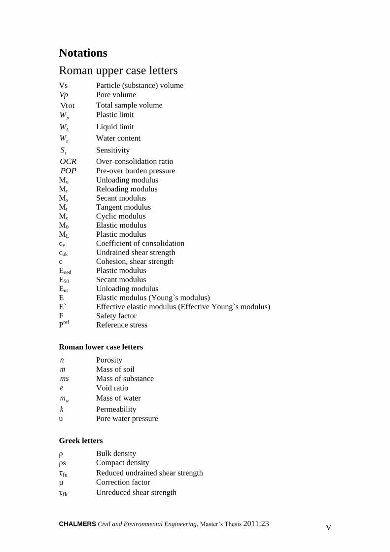
Notations
Roman upper case letters
Vs Particle (substance) volume
Vp Pore volume
Vtot Total sample volume
pW Plastic limit
LW Liquid limit
nW Water content
tS Sensitivity
OCR Over-consolidation ratio
POP Pre-over burden pressure
Mu Unloading modulus
Mr Reloading modulus
Ms Secant modulus
Mt Tangent modulus
Mc Cyclic modulus
M0 Elastic modulus
ML Plastic modulus
cv Coefficient of consolidation
cuk Undrained shear strength
c Cohesion, shear strength
Eoed Plastic modulus
E50 Secant modulus
Eur Unloading modulus
E Elastic modulus (Young`s modulus)
E` Effective elastic modulus (Effective Young`s modulus)
F Safety factor
Pref
Reference stress
Roman lower case letters
n Porosity
m Mass of soil
ms Mass of substance
e Void ratio
wm Mass of water
k Permeability
u Pore water pressure
Greek letters
ρ Bulk density
ρs Compact density
τfu Reduced undrained shear strength
µ Correction factor
τfk Unreduced shear strength
CHALMERS, Civil and Environmental Engineering, Master’s Thesis 2011:23 VI
τrem Remoulded shear strength
σ Total stresses
σ' Effective stresses
ε Strains
σ’c Over-consolidation pressure
Poisons ratio
υ Friction angle
Ψ Dilatancy angle
σ1 Major principal stress
σ3 Minor principal stress
CHALMERS, Civil and Environmental Engineering, Master’s Thesis 2011:23 1
1. Introduction
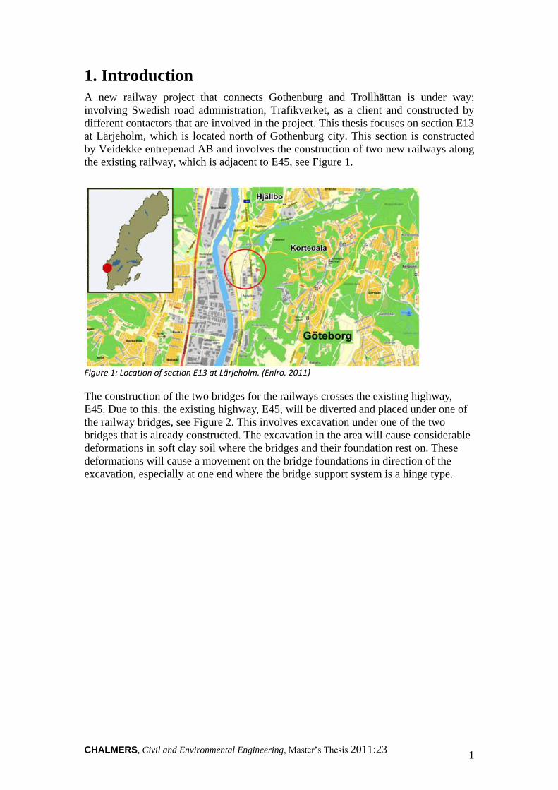
A new railway project that connects Gothenburg and Trollhättan is under way;
involving Swedish road administration, Trafikverket, as a client and constructed by
different contactors that are involved in the project. This thesis focuses on section E13
at Lärjeholm, which is located north of Gothenburg city. This section is constructed
by Veidekke entrepenad AB and involves the construction of two new railways along
the existing railway, which is adjacent to E45, see Figure 1.
Figure 1: Location of section E13 at Lärjeholm. (Eniro, 2011)
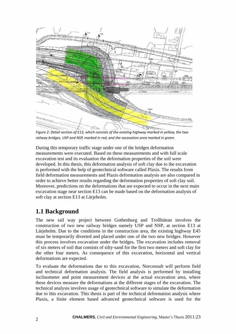
The construction of the two bridges for the railways crosses the existing highway,
E45. Due to this, the existing highway, E45, will be diverted and placed under one of
the railway bridges, see Figure 2. This involves excavation under one of the two
bridges that is already constructed. The excavation in the area will cause considerable
deformations in soft clay soil where the bridges and their foundation rest on. These
deformations will cause a movement on the bridge foundations in direction of the
excavation, especially at one end where the bridge support system is a hinge type.
CHALMERS, Civil and Environmental Engineering, Master’s Thesis 2011:23 2
Figure 2: Detail section of E13, which consists of the existing highway marked in yellow, the two
railway bridges, USP and NSP, marked in red, and the excavation area marked in green.
During this temporary traffic stage under one of the bridges deformation
measurements were executed. Based on these measurements and with full scale
excavation test and its evaluation the deformation properties of the soil were
developed. In this thesis, this deformation analysis of soft clay due to the excavation
is performed with the help of geotechnical software called Plaxis. The results from
field deformation measurements and Plaxis deformation analysis are also compared in
order to achieve better results regarding the deformation properties of soft clay soil.
Moreover, predictions on the deformations that are expected to occur in the next main
excavation stage near section E13 can be made based on the deformation analysis of
soft clay at section E13 at Lärjeholm.
1.1 Background
The new rail way project between Gothenburg and Trollhättan involves the
construction of two new railway bridges namely USP and NSP, at section E13 at
Lärjeholm. Due to the conditions in the construction area, the existing highway E45
must be temporarily diverted and placed under one of the two new bridges. However
this process involves excavation under the bridges. The excavation includes removal
of six meters of soil that consists of silty-sand for the first two meters and soft clay for
the other four meters. As consequence of this excavation, horizontal and vertical
deformations are expected.
To evaluate the deformations due to this excavation, Norconsult will perform field
and technical deformation analysis. The field analysis is performed by installing
inclinometer and point measurement devices at the actual excavation area, where
these devices measure the deformations at the different stages of the excavation. The
technical analysis involves usage of geotechnical software to simulate the deformation
due to this excavation. This thesis is part of the technical deformation analysis where
Plaxis, a finite element based advanced geotechnical software is used for the
CHALMERS, Civil and Environmental Engineering, Master’s Thesis 2011:23 3
deformation simulation. The simulation in thesis is performed by using field and
laboratory data of soil parameters of the excavation area and by using these parameter
values as an input for Plaxis and interpreting the output values. In the simulation two
different soil models are used, namely Mohr coulomb and hardening soil model in
order to take into account the mechanical deformation properties of soil and obtain a
better and realistic result from the analysis. The outputs from Plaxis deformation
simulation is compared with results from the field measurements in order to control
the different soil parameters and empirical approaches used in the analysis.
Furthermore, parameter analysis is performed to see which soil parameter and factor
has significant influence on the deformation of soft clay. Finally, conclusions and
recommendations are made on the deformation of soft soil due to unloading based the
field and technical deformation analysis.
1.2 Aim
The aim of this project is to study in depth the deformation properties of soft clay due
to excavation, and to use this analysis as a basis to decide which soil parameter has
substantial influence on the deformation of soft clay. Special attention is given to the
stiffness Modulus that will contribute much in the deformation analysis and computer
simulation. This is because, in this case, due to unloading of the soil, the stiffness
modulus is expected to be different from the one that is obtained from the oedometer
or triaxial laboratory test. Different empirical approaches are used to get a reasonable
and accurate unloading modulus. Furthermore, measurement readings of deformation
on the site are compared with output from plaxis software simulation to see which
empirical approach gives better and realistic result.
1.3 Material and method
In this project different materials such as geotechnics compendium, lecture notes from
infrastructural geo engineering course, different internet sources, and different
geotechnical reading materials that are available as softcopy and hard copy at
norconsult are used. Moreover borehole data from the site and Plaxis computer
program are used for the deformation analysis.
1.4 Delimitation
Section E13 at Lärjeholm or the excavation area under the bridge, where the existing
E45 will be diverted and placed under the bridge, is the area where this thesis mainly
focuses on. Only this section will be discussed in this project, and prediction on the
other excavations will be made based upon the analysis in this section.
CHALMERS, Civil and Environmental Engineering, Master’s Thesis 2011:23 4
2. Theory
In this chapter, basic theories and literature reviews that are relevant to this thesis are
presented. The basic theories behind the deformation properties of soil, field and
laboratory tests are discussed. The empirical approaches that available to control
investigated soil parameters are also discussed. Finally, some concepts about Plaxis,
software used for deformation analysis, are discussed.
2.1 Properties of soil
The loose part of the earth´s crust consists of different soil types, for instance, sand,
till and clay. These different types of soils are made up of two different kinds of
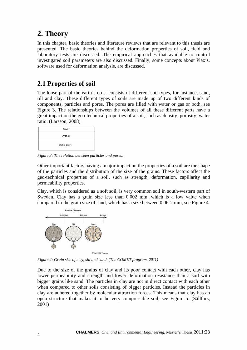
components, particles and pores. The pores are filled with water or gas or both, see
Figure 3. The relationships between the volumes of all these different parts have a
great impact on the geo-technical properties of a soil, such as density, porosity, water
ratio. (Larsson, 2008)
Figure 3: The relation between particles and pores.
Other important factors having a major impact on the properties of a soil are the shape
of the particles and the distribution of the size of the grains. These factors affect the
geo-technical properties of a soil, such as strength, deformation, capillarity and
permeability properties.
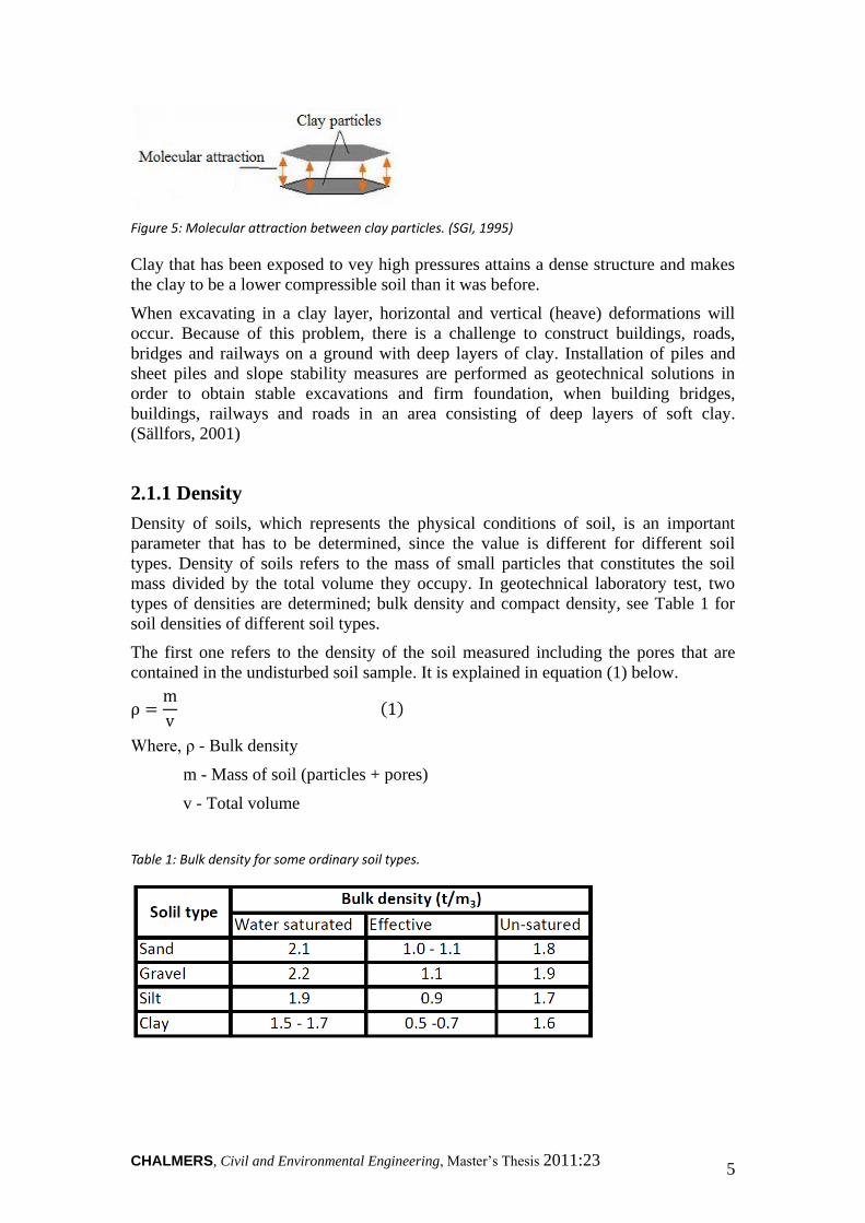
Clay, which is considered as a soft soil, is very common soil in south-western part of
Sweden. Clay has a grain size less than 0.002 mm, which is a low value when
compared to the grain size of sand, which has a size between 0.06-2 mm, see Figure 4.
Figure 4: Grain size of clay, silt and sand. (The COMET program, 2011)
Due to the size of the grains of clay and its poor contact with each other, clay has
lower permeability and strength and lower deformation resistance than a soil with
bigger grains like sand. The particles in clay are not in direct contact with each other
when compared to other soils consisting of bigger particles. Instead the particles in
clay are adhered together by molecular attraction forces. This means that clay has an
open structure that makes it to be very compressible soil, see Figure 5. (Sällfors,
2001)
CHALMERS, Civil and Environmental Engineering, Master’s Thesis 2011:23 5
Figure 5: Molecular attraction between clay particles. (SGI, 1995)
Clay that has been exposed to vey high pressures attains a dense structure and makes
the clay to be a lower compressible soil than it was before.
When excavating in a clay layer, horizontal and vertical (heave) deformations will
occur. Because of this problem, there is a challenge to construct buildings, roads,
bridges and railways on a ground with deep layers of clay. Installation of piles and
sheet piles and slope stability measures are performed as geotechnical solutions in
order to obtain stable excavations and firm foundation, when building bridges,
buildings, railways and roads in an area consisting of deep layers of soft clay.
(Sällfors, 2001)
2.1.1 Density
Density of soils, which represents the physical conditions of soil, is an important
parameter that has to be determined, since the value is different for different soil
types. Density of soils refers to the mass of small particles that constitutes the soil
mass divided by the total volume they occupy. In geotechnical laboratory test, two
types of densities are determined; bulk density and compact density, see Table 1 for
soil densities of different soil types.
The first one refers to the density of the soil measured including the pores that are
contained in the undisturbed soil sample. It is explained in equation (1) below.
( )
Where, ρ - Bulk density
m - Mass of soil (particles + pores)
v - Total volume
Table 1: Bulk density for some ordinary soil types.

CHALMERS, Civil and Environmental Engineering, Master’s Thesis 2011:23 6
Meanwhile, the latter density refers to the density of the particles, which is the mass
of the substance divided by the volume of the substance. See equation (2) below.
( )
Where, ρs - Compact density
ms - Mass of substance (particles)
vs– Volume of substance
2.1.2 Porosity
A soil consists of particles and pores, which are filled with water or/and gas as stated
in the introduction of this chapter. Porosity of soils, n is determined by dividing the
volume of the pores in a soil sample with the total volume of the soil sample, see
equation (3) below.
( )
Where, n - Porosity
Vp - Pore volume
Vtot - Total sample volume
The relation between the volume of the pores and the volume of the particles (solid
part of the soil) can be seen in equation (4).
( )
Where, e - Pore ratio
Vp - Pore volume
Vs - Particle (substance) volume
The upper two equations can be combined and equation (5) shows the relation.
( )
2.1.3 Consistency limits
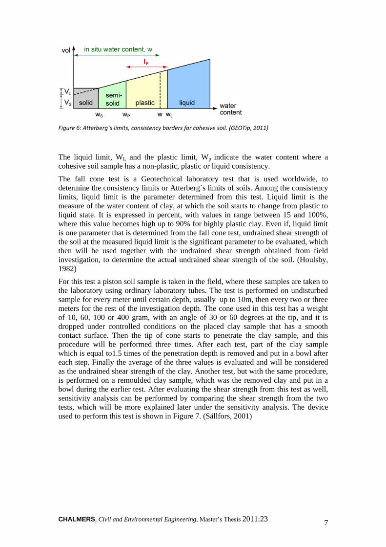
The consistency in a clay sample is strongly dependent on the water content. The
consistency can be plastic, liquid etc. Figure 6 shows the borders between different
consistency limits, also called Atterberg`s limits of soils.
CHALMERS, Civil and Environmental Engineering, Master’s Thesis 2011:23 7
Figure 6: Atterberg`s limits, consistency borders for cohesive soil. (GEOTip, 2011)
The liquid limit, WL and the plastic limit, Wp indicate the water content where a
cohesive soil sample has a non-plastic, plastic or liquid consistency.
The fall cone test is a Geotechnical laboratory test that is used worldwide, to
determine the consistency limits or Atterberg`s limits of soils. Among the consistency
limits, liquid limit is the parameter determined from this test. Liquid limit is the
measure of the water content of clay, at which the soil starts to change from plastic to
liquid state. It is expressed in percent, with values in range between 15 and 100%,
where this value becomes high up to 90% for highly plastic clay. Even if, liquid limit
is one parameter that is determined from the fall cone test, undrained shear strength of
the soil at the measured liquid limit is the significant parameter to be evaluated, which
then will be used together with the undrained shear strength obtained from field
investigation, to determine the actual undrained shear strength of the soil. (Houlsby,
1982)
For this test a piston soil sample is taken in the field, where these samples are taken to
the laboratory using ordinary laboratory tubes. The test is performed on undisturbed
sample for every meter until certain depth, usually up to 10m, then every two or three
meters for the rest of the investigation depth. The cone used in this test has a weight
of 10, 60, 100 or 400 gram, with an angle of 30 or 60 degrees at the tip, and it is
dropped under controlled conditions on the placed clay sample that has a smooth
contact surface. Then the tip of cone starts to penetrate the clay sample, and this
procedure will be performed three times. After each test, part of the clay sample
which is equal to1.5 times of the penetration depth is removed and put in a bowl after
each step. Finally the average of the three values is evaluated and will be considered
as the undrained shear strength of the clay. Another test, but with the same procedure,
is performed on a remoulded clay sample, which was the removed clay and put in a
bowl during the earlier test. After evaluating the shear strength from this test as well,
sensitivity analysis can be performed by comparing the shear strength from the two
tests, which will be more explained later under the sensitivity analysis. The device
used to perform this test is shown in Figure 7. (Sällfors, 2001)

CHALMERS, Civil and Environmental Engineering, Master’s Thesis 2011:23 8
Figure 7: Measuring equipment for fall cone test (Houlsby, 1982)
A correction factor µ, which is a function of liquid limit, see equation (6), will be
applied in order to reduce the undrained shear strength obtained from the fall cone
test, since the values obtained from the test has shown to be higher than the actual
undrained shear strength of the clay.
( )
Where, τfu - Corrected undrained shear strength, same as cuk
µ - Correction factor = (0.43/WL)0.45
τfk - Uncorrected shear strength from fall cone test
2.1.4 Natural water content
In soil mechanics, natural water content refers to the quantity of water that is found in
a given soil sample. It is expressed as the ratio between the weights of water in the
soil to the weight of the solid soil, see equation (7).
( )
Where, wn - Water content
mw - Mass of water
ms - Mass of solid soil (substance)
2.1.5 Shear strength (Vane, cone, CPT, shear test)
Shear strength of soil refers to shear resistance of soil to certain magnitude of shear
stress. The shear strength of soil depends on many factors. One factor is soil
composition, which refers to the mineralogy, grain size distribution and shape of
particles of the soil mass. Additionally, the structure or arrangement of particles of
soil layers and joints affects the shear resistance of the soil. Another factor is the
initial soil state of the soil, which refers to the stress history of the soil that the soil has
been subjected to. Normally there are two ways of modelling the shear strength,

CHALMERS, Civil and Environmental Engineering, Master’s Thesis 2011:23 9
namely as undrained and drained shear strength. The first one refers to the shear
strength obtained from soil that passed undrained stress path where water was not
allowed to flow into or out of the soil. Meanwhile, the latter one applies to shear
strength of soil at which either no water exists or the pore water pressure dissipates
during the shearing action.
The shear strength of soil is evaluated by performing field and laboratory tests. Cone
penetration test and vane shear tests are in-situ tests where tip and skin resistance of
the soil when subjected to loading from devices are measured and converted to shear
strength value through empirical correlation. Direct shear test, a laboratory test, is also
another test to determine the shear strength of a soil. The test is performed in such a
way that undisturbed soil sample is placed inside a shear box and shear force at a
confining vertical pressure is applied until the soil sample fails. Stress-strain curves
are collected at different intervals for the confining pressure. The rate of strain is
varied in order to take into account undrained and drained conditions. Shear strength
parameters cohesion (c) and internal angle of friction (υ) are evaluated at failure.
2.1.6 Sensitivity
Sensitivity test is performed in soft plastic soils that are expected to show a significant
reduction of shear strength when subjected to shearing action. As stated earlier,
sensitivity test is carried out during fall cone test, and it is defined by the ratio of the
undisturbed shear strength divided by the remoulded shear strength, see equation (8)
below. (Sällfors, 2001)
( )
Where, St - Sensitivity
τfu - Undisturbed shear strength
τrem - Remoulded shear strength
2.1.7 Effective stress and pre-consolidation pressure
The total stress in the soil is a function of the stress transmitted by the soil particles
and the water. The constituent of the total stress carried by the soil particles is called
effective stress, σ’ and the other constituent is called pore water pressure or pore
pressure, u see equation (9). The values of these stress components are evaluated by
plotting the accumulated unit weight of the soil and unit weight of water as a function
of depth.
( )
Where, σ - Total stress
σ'- Effective stress
u - Pore water pressure
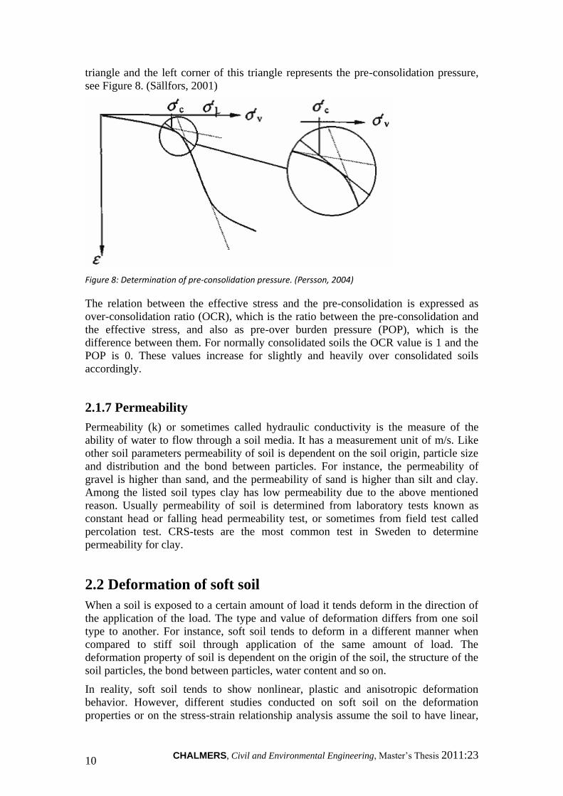
The pre-consolidation pressure refers to the maximum vertical stress that the soil has
been subjected in the past. This parameter is determined from the oedometer
laboratory test. It is the breaking point in the stress strain plot obtained from this test.
The tangent lines drawn in this bi-linear curve intersect at a point forming an isosceles
CHALMERS, Civil and Environmental Engineering, Master’s Thesis 2011:23 10
triangle and the left corner of this triangle represents the pre-consolidation pressure,
see Figure 8. (Sällfors, 2001)
Figure 8: Determination of pre-consolidation pressure. (Persson, 2004)
The relation between the effective stress and the pre-consolidation is expressed as
over-consolidation ratio (OCR), which is the ratio between the pre-consolidation and
the effective stress, and also as pre-over burden pressure (POP), which is the
difference between them. For normally consolidated soils the OCR value is 1 and the
POP is 0. These values increase for slightly and heavily over consolidated soils
accordingly.
2.1.7 Permeability
Permeability (k) or sometimes called hydraulic conductivity is the measure of the
ability of water to flow through a soil media. It has a measurement unit of m/s. Like
other soil parameters permeability of soil is dependent on the soil origin, particle size
and distribution and the bond between particles. For instance, the permeability of
gravel is higher than sand, and the permeability of sand is higher than silt and clay.
Among the listed soil types clay has low permeability due to the above mentioned
reason. Usually permeability of soil is determined from laboratory tests known as
constant head or falling head permeability test, or sometimes from field test called
percolation test. CRS-tests are the most common test in Sweden to determine
permeability for clay.
2.2 Deformation of soft soil
When a soil is exposed to a certain amount of load it tends deform in the direction of
the application of the load. The type and value of deformation differs from one soil
type to another. For instance, soft soil tends to deform in a different manner when
compared to stiff soil through application of the same amount of load. The
deformation property of soil is dependent on the origin of the soil, the structure of the
soil particles, the bond between particles, water content and so on.
In reality, soft soil tends to show nonlinear, plastic and anisotropic deformation
behavior. However, different studies conducted on soft soil on the deformation
properties or on the stress-strain relationship analysis assume the soil to have linear,

CHALMERS, Civil and Environmental Engineering, Master’s Thesis 2011:23 11
elastic and isotropic deformation behavior, see figure 9. This is due to the fact that the
theory of elasticity is intense and easy to apply.
Figure 9: Different material models of soil behaviour: 1) linear elastic model, 2) elastic-perfectly plastic
model, 3) non-linear model, 4) elasto-plastic model. (Persson, 2004)
In analysis of deformation of soft soil, the elastic deformation limit is the pre-
consolidation or similar yield stress for drained conditions, and shear strength for
undrained conditions. Failure criterion is based up on Mohr – coulomb failure
criterion, which is determined by performing triaxial and oedometer laboratory tests.
2.2.1 Soil stiffness
The stiffness of soil is characterized by the modulus of elasticity or the so called
Young’s modulus. This stiffness parameter is usually determined from stress-strain
curve obtained from oedometer and triaxial test. The modulus depends on how the
particles of the soil are packed and organized. Soil with closely packed particles tends
to have a higher modulus value than a soil with particles not closely packed. Water
content of the soil also affects the value of modulus. Normally, low water content in
the soil leads to high soil modulus. This is due to the fact that at low water content the
water binds the particles and thus increases the effective stress among particles
through suction. Last but not least, the soil modulus depends on the pre-consolidation
pressure, which refers to the pressure or stress that the soil has been subjected to in the
past. Normally consolidated soils have lower soil modulus than over consolidated soil.
(Briaud, 2010)
To determine the value of the modulus, first, the slope from the curve is evaluated and
afterwards the modulus is calculated using empirical formulas, see Figure 10.
Figure 10: Calculation of modulus of elasticity. (Briaud, 2010)
CHALMERS, Civil and Environmental Engineering, Master’s Thesis 2011:23 12
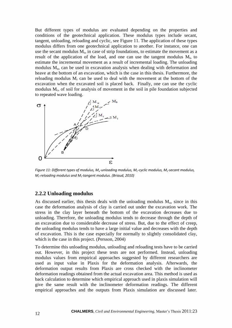
But different types of modulus are evaluated depending on the properties and
conditions of the geotechnical application. These modulus types include secant,
tangent, unloading, reloading and cyclic, see Figure 11. The application of these types
modulus differs from one geotechnical application to another. For instance, one can
use the secant modulus Ms, in case of strip foundations, to estimate the movement as a
result of the application of the load, and one can use the tangent modulus Mt, to
estimate the incremental movement as a result of incremental loading. The unloading
modulus Mu, can be used in excavation analysis when dealing with deformation and
heave at the bottom of an excavation, which is the case in this thesis. Furthermore, the
reloading modulus Mr can be used to deal with the movement at the bottom of the
excavation when the excavated soil is placed back. Finally, one can use the cyclic
modulus Mc, of soil for analysis of movement in the soil in pile foundation subjected
to repeated wave loading.
Figure 11: Different types of modulus, Mu-unloading modulus, Mc-cyclic modulus, Ms-secant modulus,
Mr-reloading modulus and Mt-tangent modulus. (Briaud, 2010)
2.2.2 Unloading modulus
As discussed earlier, this thesis deals with the unloading modulus Mu, since in this
case the deformation analysis of clay is carried out under the excavation work. The
stress in the clay layer beneath the bottom of the excavation decreases due to
unloading. Therefore, the unloading modulus tends to decrease through the depth of
an excavation due to considerable decrease of stress. But, due to the effect of creep,
the unloading modulus tends to have a large initial value and decreases with the depth
of excavation. This is the case especially for normally to slightly consolidated clay,
which is the case in this project. (Persson, 2004)
To determine this unloading modulus, unloading and reloading tests have to be carried
out. However, in this project these tests are not performed. Instead, unloading
modulus values from empirical approaches suggested by different researchers are
used as input value in Plaxis for the deformation analysis. Afterwards, the
deformation output results from Plaxis are cross checked with the inclinometer
deformation readings obtained from the actual excavation area. This method is used as
back calculation to determine which empirical approach used in plaxis simulation will
give the same result with the inclinometer deformation readings. The different
empirical approaches and the outputs from Plaxis simulation are discussed later.
CHALMERS, Civil and Environmental Engineering, Master’s Thesis 2011:23 13
Furthermore, the comparison made between the outputs from Plaxis and inclinometer
readings to determine the actual unloading modulus is also presented.
2.2.3 Deformation determination
The deformation of soil is determined by performing laboratory tests by using soil
samples collected from the field and by direct measurements in the field where the
construction is taking place. The laboratory tests include the oedometer test and
triaxial test, and the direct measurements are carried out by using devices such as
inclinometer and gauges of timber. The procedures used in these deformation
determination methods are discussed below.
2.2.3.1 Oedometer test
In geotechnical laboratory test program, the oedometer test is the common test
performed to determine the deformation properties, consolidation and swelling
parameters of soil. It involves two types of methods, namely, incremental load steps
and constant rate of strain, CRS. However, in Sweden the constant rate of strain is
more often used.
In this constant rate of strain test, CRS, different parameters of a cohesive soil are
determined. These parameters include, the pre-consolidation pressure (σ’c) which is
the maximum overburden pressure that the soil sustained in the past, coefficient of
consolidation (cv), which refers to the measure of the time it takes for a soil to
consolidate, permeability (k) or sometimes called hydraulic conductivity. Moreover,
the stiffness moduli, M0 and ML, are also evaluated from the stress versus strain
diagram. Among these parameters that are obtained from this test, this master’s thesis
focuses on the effective stresses and the stiffness modulus, which play vital role in
determination of the deformation properties of clay . The other parameters will be
used as input data in different soil models in plaxis computer simulation.
2.2.3.2 Triaxial test
When the deformation analysis of soil is performed by an advanced soil model in
Plaxis there is a need of a triaxial test. This because advanced models require more
input of material data, for instance hardening soil model requires input of three
modules, such as Eoed obtained from CRS test, E50 and Eur, which are obtained by
performing a triaxial test.
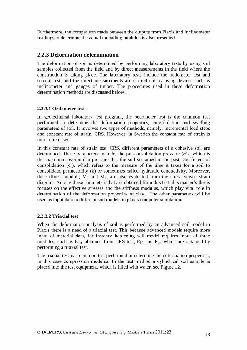
The triaxial test is a common test performed to determine the deformation properties,
in this case compression modulus. In the test method a cylindrical soil sample is
placed into the test equipment, which is filled with water, see Figure 12.
CHALMERS, Civil and Environmental Engineering, Master’s Thesis 2011:23 14
Figure 12: The trixial test method equipment. (SGI, 1995)
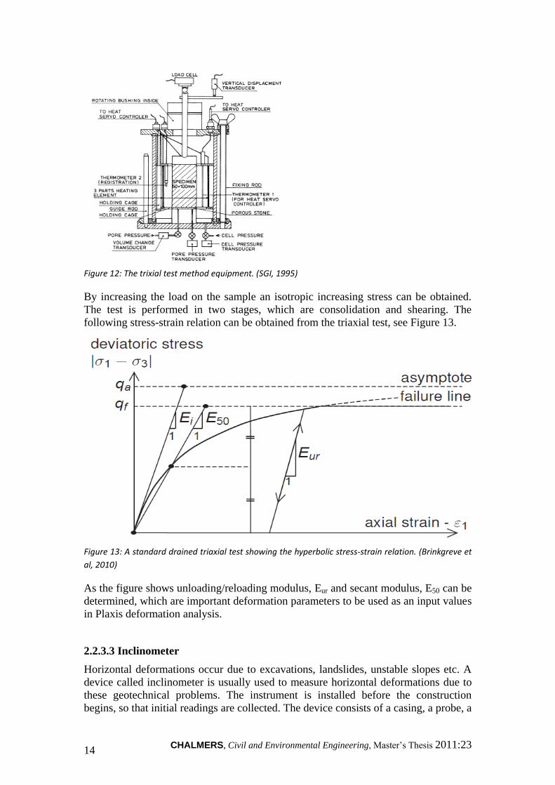
By increasing the load on the sample an isotropic increasing stress can be obtained.
The test is performed in two stages, which are consolidation and shearing. The
following stress-strain relation can be obtained from the triaxial test, see Figure 13.
Figure 13: A standard drained triaxial test showing the hyperbolic stress-strain relation. (Brinkgreve et
al, 2010)
As the figure shows unloading/reloading modulus, Eur and secant modulus, E50 can be
determined, which are important deformation parameters to be used as an input values
in Plaxis deformation analysis.
2.2.3.3 Inclinometer
Horizontal deformations occur due to excavations, landslides, unstable slopes etc. A
device called inclinometer is usually used to measure horizontal deformations due to
these geotechnical problems. The instrument is installed before the construction
begins, so that initial readings are collected. The device consists of a casing, a probe, a

CHALMERS, Civil and Environmental Engineering, Master’s Thesis 2011:23 15
control cable and a unit. Each component contributes some to perform measurement,
see Figure 14. (Brouwer, 2007)
Figure 14: The inclinometer device. (Brouwer, 2007)
The casing, see Figure 15, is installed in a vertical borehole, which is situated in the
soil layer where the deformations are expected. It is installed down to a depth where
no deformations are expected to occur, and this is done so the casing will not rotate. It
can also be installed in a way that it reaches the firm bottom (bedrock). (Brouwer,
2007)
Figure 15: The illustrations show a casing. (Brouwer, 2007)
When the ground moves, the casing anchored in the borehole will also move and by
measuring the inclination and comparing to initial readings of the movement, the
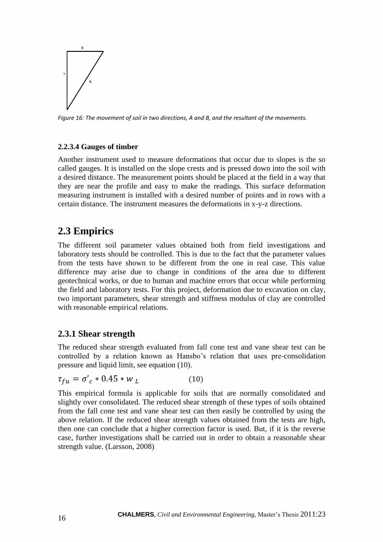
deformation is obtained. Usually the measurements are done twice by pulling up the
inclinometer probe from bottom of the casing to top. The first measurement is done
parallel to the inclinometer`s wheel, which is the direction of the expected movement
of the ground (A) and the second one is performed perpendicular to the wheel (B), see
Figure 16. The movement of the ground is obtained by calculating the resultant of A
and B axis. (Brouwer, 2007)
CHALMERS, Civil and Environmental Engineering, Master’s Thesis 2011:23 16
Figure 16: The movement of soil in two directions, A and B, and the resultant of the movements.
2.2.3.4 Gauges of timber
Another instrument used to measure deformations that occur due to slopes is the so
called gauges. It is installed on the slope crests and is pressed down into the soil with
a desired distance. The measurement points should be placed at the field in a way that
they are near the profile and easy to make the readings. This surface deformation
measuring instrument is installed with a desired number of points and in rows with a
certain distance. The instrument measures the deformations in x-y-z directions.
2.3 Empirics
The different soil parameter values obtained both from field investigations and
laboratory tests should be controlled. This is due to the fact that the parameter values
from the tests have shown to be different from the one in real case. This value
difference may arise due to change in conditions of the area due to different
geotechnical works, or due to human and machine errors that occur while performing
the field and laboratory tests. For this project, deformation due to excavation on clay,
two important parameters, shear strength and stiffness modulus of clay are controlled
with reasonable empirical relations.
2.3.1 Shear strength
The reduced shear strength evaluated from fall cone test and vane shear test can be
controlled by a relation known as Hansbo’s relation that uses pre-consolidation
pressure and liquid limit, see equation (10).
( )
This empirical formula is applicable for soils that are normally consolidated and
slightly over consolidated. The reduced shear strength of these types of soils obtained
from the fall cone test and vane shear test can then easily be controlled by using the
above relation. If the reduced shear strength values obtained from the tests are high,
then one can conclude that a higher correction factor is used. But, if it is the reverse
case, further investigations shall be carried out in order to obtain a reasonable shear
strength value. (Larsson, 2008)
CHALMERS, Civil and Environmental Engineering, Master’s Thesis 2011:23 17
2.3.2 Modulus
The stiffness modulus, M0 obtained from the CRS-test should be controlled, since the
value obtained from the test can be different from the actual value in field. Especially
the unloading modulus, the modulus of soil where there is considerable excavation, is
expected to have a higher value than the one obtained from the CRS test, since the
shear strain around the excavation area is expected to be small. To estimate a
reasonable value of the unloading modulus, different empirical approaches are
proposed by different persons. These empirical approaches use different soil
parameters from the lab and field tests.
The first approach uses pre-consolidation pressure as a parameter for the empirics see
equation (11). This is the equation used in the tender document for the actual case to
perform the deformations analysis.
( )
The second approach used in this thesis to obtain the compression modulus, uses the
undrained shear strength as a parameter, see equation (12). This empiric approach is
only used in hardening soil model.
( )
The other empirical relation uses a factor to increase the oedometer modulus; Mo,
where it is not possible to perform unloading and reloading test to determine the real
modulus, see equation (13) (Sällfors 2001).
( ) ( )
Another empirical approach to estimate the unloading modulus of clay is proposed by
Jenny Persson, based on field tests from the construction site at Lilla Bommen. In this
approach, the unloading modulus is estimated by taking the maximum of two
formulas that have change in value of OCR range of 1.5 to 2 see equation (14).
{
(
)
( ) ( )
Where the values, A = 1500 and as is in the range of 0.0025 to 0.005.
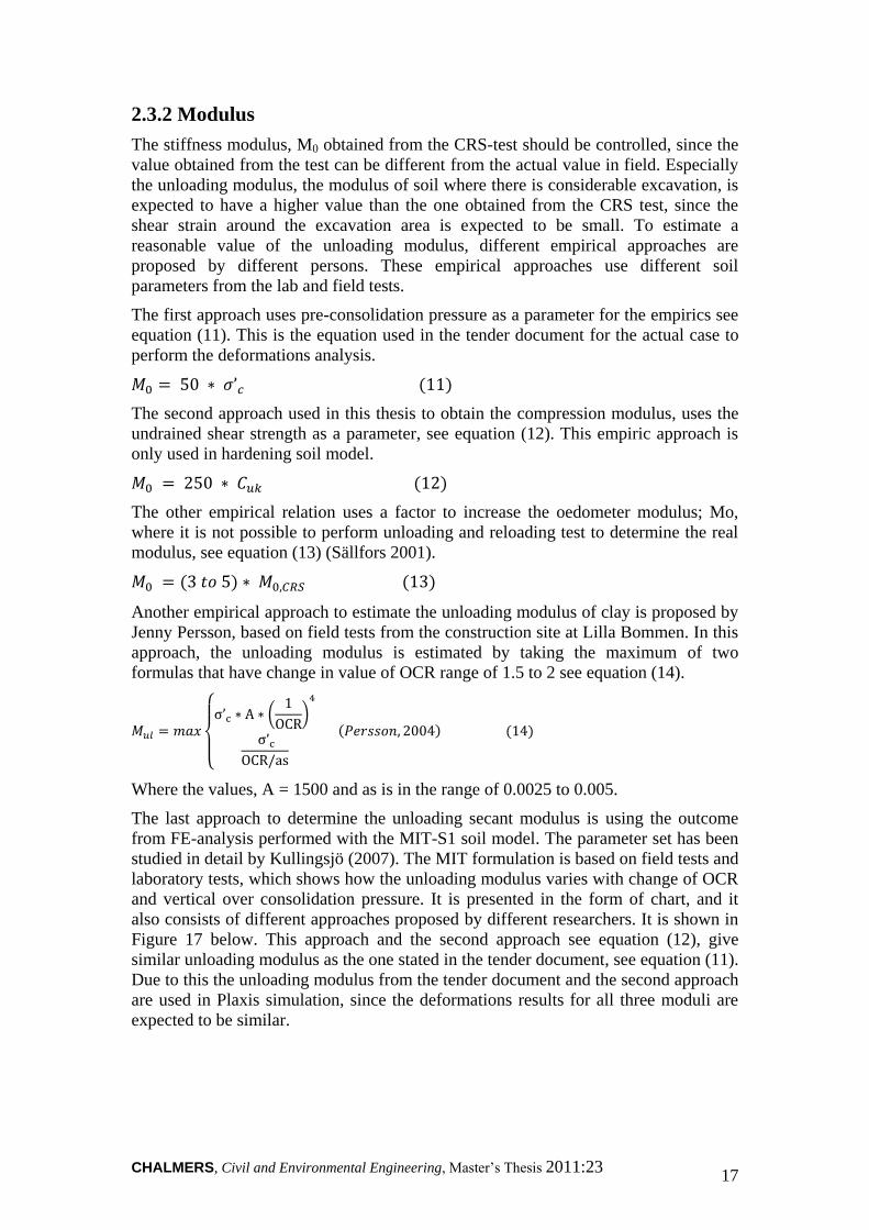
The last approach to determine the unloading secant modulus is using the outcome
from FE-analysis performed with the MIT-S1 soil model. The parameter set has been
studied in detail by Kullingsjö (2007). The MIT formulation is based on field tests and
laboratory tests, which shows how the unloading modulus varies with change of OCR
and vertical over consolidation pressure. It is presented in the form of chart, and it
also consists of different approaches proposed by different researchers. It is shown in
Figure 17 below. This approach and the second approach see equation (12), give
similar unloading modulus as the one stated in the tender document, see equation (11).
Due to this the unloading modulus from the tender document and the second approach
are used in Plaxis simulation, since the deformations results for all three moduli are
expected to be similar.
CHALMERS, Civil and Environmental Engineering, Master’s Thesis 2011:23 18
Figure 17: Comparison of different approaches for unloading modulus (Kullingsjö, 2007)
2.4 Plaxis
In different geotechnical applications, Plaxis, a two dimensional finite element based
computer program, is used for simulation purpose. This sophisticated computer
program is mainly used for analysis of deformation and stability. It has advantageous
feature that enables users to choose different soil models, which is dependent on
mechanical deformation behaviours of soil, for the simulation. In this project, among
the different soil models, Mohr coulomb (MC) and hardening soil (HS) models are
chosen for the deformation analysis. The basic principles and assumptions in these
models are discussed in detail later.
2.4.1 Input
The purpose of the input program is to create the geotechnical finite element model, to
define and assign material properties and to generate the initial stress with in the soil
layers and boundary condition. To create the geometry of the model, points, lines, and
clusters (areas) are used. Different types of geotechnical and structural elements can
be inserted into the model. The fixity and support system of the elements are also
defined depending on the conditions of the application. Additionally, different types
of loads and boundary conditions can be defined. The material properties definition
stage involve inserting different soil parameters like young’s modulus (E),
cohesion(c), poisons ratio (υ), friction angle (υ), and dilatancy angle (Ψ) into the

CHALMERS, Civil and Environmental Engineering, Master’s Thesis 2011:23 19
program. These soil parameters can be different for different soil models. The method
of analysis, drained or undrained, is also defined here. Once all these are performed, a
mesh in form of small triangles connected to each other can be generated. The finer
the mesh is, the complexity of analysis of the model increases, but the accuracy, on
the other hand also increases. The phreatic level that shows the level and orientation
of the ground water is another important aspect to be defined in the input program.
Before proceeding to the calculation part, initial stress level of the soil is generated by
using the Ko- procedure or the gravity loading. (Brinkgreve et al, 2010)
2.4.2 Calculation
The calculation program is the part of the whole simulation where the analysis of the
created model is performed. The procedure is started by defining the initial stage or
the already created finite element model in the input program. Then the other
construction stages can be defined, otherwise the program only simulates the model
defined from the input program. Plaxis offers three types of calculation modes for the
users. These include, plastic, where the deformation is expected to be elastic-plastic,
consolidation, where the development of or dissipation of excess pore pressure in the
clay is considered, and phi-c reduction, a safety analysis by reducing the strength
parameters of the soil. In this calculation part there are also load stepping and control,
and load incremental multipliers option where the user can insert appropriate value
depending on the conditions of the application. Additionally, sensitivity analysis can
be performed to determine the influence of individual parameters on the output of the
simulation. Before the final calculation is started, specific points can be selected to
generate load-displacement curves and stress path or stress strain curves for those
points. (Bringreve et al, 2010)
2.4.3 Output
In Plaxis, the results from the overall simulation can be obtained from the output
program. It mainly emphasizes on results of generated input data and finite element
based calculation. The outputs can be in the form of plots of full model, or plots of
special objects of the model and in the form of tables. For a specific output, the result
can be presented in the form of arrows, contours and shadings. Different types of
outputs can be obtained from the simulation, choosing the important results will
depend on the purpose of the simulation and the choice professional performing the
simulation. The outputs obtained from Plaxis include, deformed mesh of the whole
model, different types of deformations and strains and effective and total stresses. For
structural and geotechnical elements, the possible outputs from the simulation consist
of deformations, axial shear forces and bending moments. For a particular section,
where results from that section are relevant, Plaxis offers a way to view the outputs in
that section inform of cross-section. Load-displacement curves and time-displacement
curves can also be generated for those specific points which were selected before
running the calculation. All the relevant outputs from the simulation can be
documented in report form. (Bringreve et al, 2010)

CHALMERS, Civil and Environmental Engineering, Master’s Thesis 2011:23 20
2.4.4 Soil models
In Plaxis, different soil models are available in order to carryout appropriate
simulation for different types of geotechnical applications. These models include the
Mohr coulomb (MC), joint rock (JR), hardening soil (HS), soft soil (SS), and
modified cam-clay model. As mentioned earlier, among the listed soil models, for this
project, Mohr coulomb (MC) and hardening soil (HS) are chosen to be used. This is
due to these models are assumed have features that take into consideration the
characteristics and aim of this project.
2.4.4.1 Mohr coulomb (MC)
The main concept behind the Mohr coulomb method of analysis is that failure in soils
occurs when the applied shear stress is equal to the shear strength of the soil. As
shown in figure (18), the Mohr circle is drawn on Cartesian coordinate of principal
stress versus shear stress. Failure in the soil occurs when the Mohr circle touches the
failure envelope line. By performing laboratory tests under undrained conditions the
shear stress, τf is equal to the undrained shear strength, cuk at failure. It can be
explained with equation (15).
( ) ( )
σ1 - Major principal stress in the vertical direction
σ3 - Minor principal stress in the horizontal direction
The cohesion c’ and the friction angle υ’ can be determined from the failure envelope
line from laboratory tests performed under drained conditions. The shear strength will
be a function of the cohesion c’ and the friction angle υ’ see equation (16).
( )
Figure 18: Mohr coulomb failure criterion with effective and undrained strength parameters.
(Bringreve et al, 2010)

CHALMERS, Civil and Environmental Engineering, Master’s Thesis 2011:23 21
Mohr coulomb is a linear elastic perfectly plastic model, which means that this model
describes material behavior as elastic within a certain defined area and outside of it
plastic, sees Figure 19.
Figure 19: The figure shows the main idea of an elastic perfectly plastic soil model. (Bringreve et al,
2010)
The calculations in a Plaxis simulation by using Mohr coulomb model are fast and
therefore the model is usually used to obtain a first view of the problem. Five different
parameters are required to perform a simulation in Plaxis software by using Mohr
coulomb. The parameters required are the following; Young`s modulus E, poison`s
ratio υ, friction angle υ, cohesion c and angle of dilantancy ψ. The selected modulus
of elasticity, E is an average value of the modulus, which increases linearly with depth
by an increment Eincrement. The modulus of elasticity (Young`s modulus) is obtained
from a triaxial test or a CRS-test. If the modulus is obtained by use of a CRS-test, the
modulus, Eeod has to be transformed to an elasticity modulus, E by the equation (17).
( )
( ) ( ) ( )
If effective values of elasticity modulus, E and poison`s ratio, υ are used in Plaxis
software to perform a simulation, the equation (18) has to be used to transform the
elasticity modulus into an effective one. (Bringreve et al, 2010)
( )
( )
2.4.4.2 Hardening soil model (HS)
Hardening soil model is an advanced soil model which is used to analyze the non-
linear behavior of soil by taking into account a change of the stiffness modulus by a
change of the soil stresses due to compression and/or shearing of the soil. This feature
makes this model to be different from Mohr coulomb model which assumes the soil to
have elastic-perfectly plastic behavior. The hardening soil model also allows a more
precise soil modeling by taking into consideration the pre-consolidation pressure. In
Plaxis this can be performed by use of OCR (Over Consolidation Ratio) and POP (Pre
Overburden Pressure), see Figure 20.

CHALMERS, Civil and Environmental Engineering, Master’s Thesis 2011:23 22
Figure 20: The definition of over consolidation ratio by OCR and POP. (Bringreve et al, 2010)
The insertion of the pre-consolidation pressure into the model is based on the fact that
for stresses higher than the pre-consolidation pressure the stress strain curve gives a
modulus, ML that is smaller than the elastic modulus M0, see Figure 21.
Figure 21: Stiffness modulus at elastic (M0) and plastic (ML) region obtained from CRS test.
The modulus in the hardening soil model is described more accurately by adding three
moduli; Eur, which refers to reloading/unloading modulus and E50 and Eoed. E50 refers
to secant modulus from tri-axial test and Eoed refers to tangent modulus that
corresponds to a modulus for stresses higher than the pre-consolidation pressure
evaluated from the CRS test, see figure above. (Bringreve et al, 2010)
These moduli are stress dependent and in the following formulas the change of the
three moduli can be observed by the change of soil stress (by the depth), see the
equations (19), (20), & (21) below. (Bringreve et al, 2010)
(
)
( )
(
)
( )
CHALMERS, Civil and Environmental Engineering, Master’s Thesis 2011:23 23
(
)
( )
In the above mentioned formulas the Eref
is the reference Young`s modulus and pref
is
reference stress for the stiffness and is set to 100 kPa, as a default value in Plaxis.
Usually Eurref
is set to three times E50ref
and Eeodref
is set to be equal to E50ref
as a
default value of the Plaxis software. However Plaxis cannot handle to big ratios
between E50ref
and Eeodref
and therefore Plaxis software will sometimes recommend a
value of one of the modulus to use. The exponent, m, is a factor that regulates the
stress-dependence of the modulus. For soft soils the factor is set to 1 and for sands it
is set to value from 0.5 to 1. In the formulas it can also be noticed that Eoed is
dependent of the major principal stress σ1, Eur and E50 are dependent on the minor
principal stress σ3. The following formula is used to determine the horizontal stress,
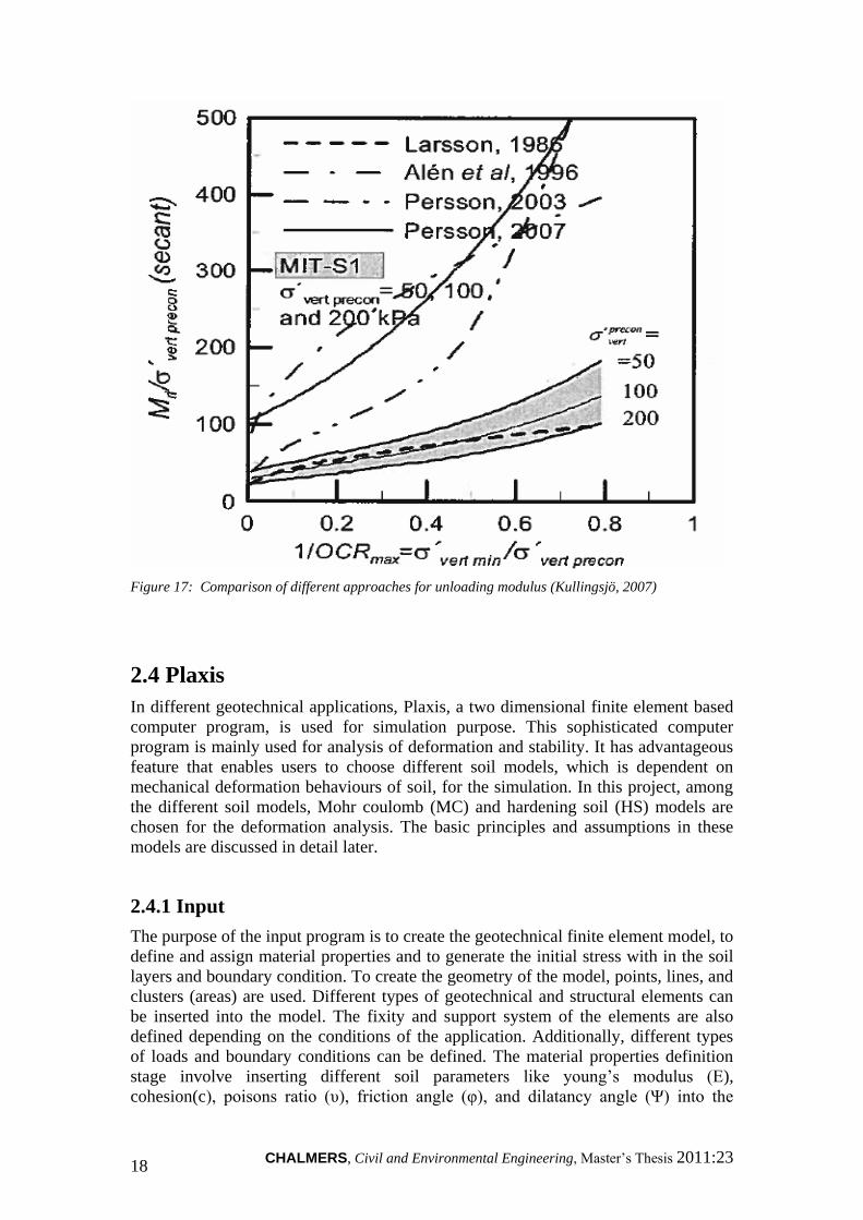
see equation (22). (Bringreve et al, 2010)
( )
Figure 22 shows the vertical and horizontal stresses varying with depth and also
which depth Pref
= 100 kPa corresponds to.
Figure 22: Effective vertical, horizontal stresses and reference stress.
Poisson`s ratio for unloading/reloading and the soil pressure coefficient, K0 are other
parameters needed to describe the deformation properties of a soil by use of hardening
soil model.

CHALMERS, Civil and Environmental Engineering, Master’s Thesis 2011:23 24
The failure parameters in this model are the same as the parameters for failure in
Mohr coulomb soil model. These include friction angle, υ, cohesion, c, and angle of
dilantancy, ψ. Due to this a safety analysis in hardening soil model will give the same
safety factor as the one obtained from Mohr Coulomb soil model. (Brinkgreve et al,
2010)
CHALMERS, Civil and Environmental Engineering, Master’s Thesis 2011:23 25
3. Deformations analysis of section E13
In this chapter, area description, soil profile and properties of different soil parameters
that are relevant to this thesis are presented. The excavation procedure is also
described in this chapter and in the end the deformation measurement is presented.
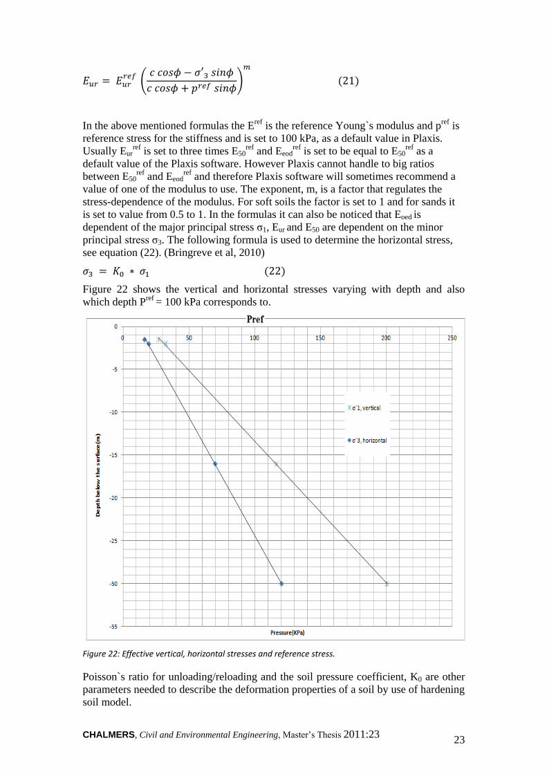
3.1 Area description
The bridge, where the excavation is taking place, is located in the stretch km 471+600
– 472+100, see drawing below. It is decided to use the field and laboratory data from
boreholes 71003, FB41, 71007 and SYD. These boreholes were selected, because of
their close proximity to the section and because they are located in the actual stretch,
in which the bridge and the excavation are supposed to be designed and performed
for. This is shown in Figure 23.
Figure 23: The red circles shows the selected boreholes, 71003, FB41, 71007 and Syd.
3.2 Topography
The area, where the excavation is taking place is located on the east side of Göta
River. The area is characterised by its low-lying landscape. The level of the ground in
the specific stretch varies from +1 meter to +3 meters above sea level.
3.3 Pore water pressure
The pore water pressure investigation has been performed 4-6 times at different
seasons of the year in order to take into account the pore pressure seasonal variation.
The result obtained from the pore water measurements in the stretch km 471+600 –
472+100 shows that the level of the groundwater begins at level +1.5, which means
1.5 meters below the ground surface. The results obtained also show that the pore
pressure is hydrostatic from level +1.5, where the groundwater begins, to level -3.
From the level -3, which is 6 meters below the ground surface the pore pressure
increases with 10.5 kPa/m.
CHALMERS, Civil and Environmental Engineering, Master’s Thesis 2011:23 26
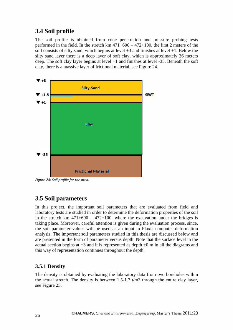
3.4 Soil profile
The soil profile is obtained from cone penetration and pressure probing tests
performed in the field. In the stretch km 471+600 – 472+100, the first 2 meters of the
soil consists of silty sand, which begins at level +3 and finishes at level +1. Below the
silty sand layer there is a deep layer of soft clay, which is approximately 36 meters
deep. The soft clay layer begins at level +1 and finishes at level -35. Beneath the soft
clay, there is a massive layer of frictional material, see Figure 24.
Figure 24: Soil profile for the area.
3.5 Soil parameters
In this project, the important soil parameters that are evaluated from field and
laboratory tests are studied in order to determine the deformation properties of the soil
in the stretch km 471+600 – 472+100, where the excavation under the bridges is
taking place. Moreover, careful attention is given during the evaluation process, since,
the soil parameter values will be used as an input in Plaxis computer deformation
analysis. The important soil parameters studied in this thesis are discussed below and
are presented in the form of parameter versus depth. Note that the surface level in the
actual section begins at +3 and it is represented as depth ±0 m in all the diagrams and
this way of representation continues throughout the depth.
3.5.1 Density
The density is obtained by evaluating the laboratory data from two boreholes within
the actual stretch. The density is between 1.5-1.7 t/m3 through the entire clay layer,
see Figure 25.
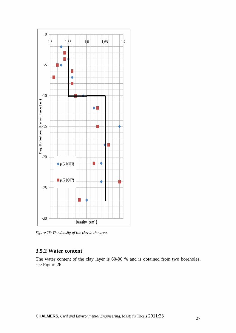
CHALMERS, Civil and Environmental Engineering, Master’s Thesis 2011:23 27
Figure 25: The density of the clay in the area.
3.5.2 Water content
The water content of the clay layer is 60-90 % and is obtained from two boreholes,
see Figure 26.
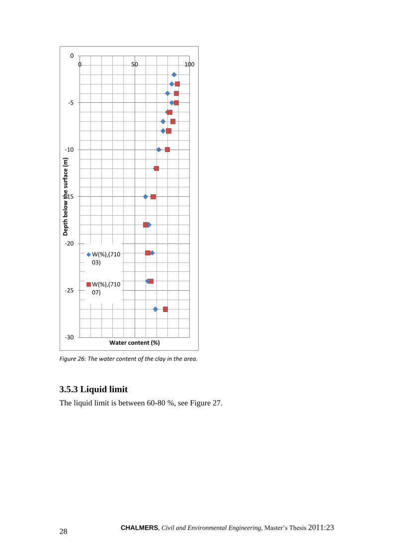
CHALMERS, Civil and Environmental Engineering, Master’s Thesis 2011:23 28
Figure 26: The water content of the clay in the area.
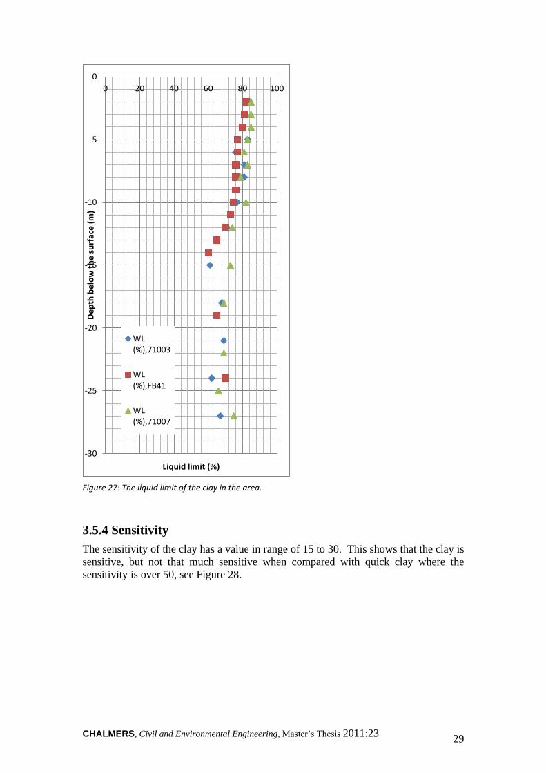
3.5.3 Liquid limit
The liquid limit is between 60-80 %, see Figure 27.
-30
-25
-20
-15
-10
-5
0
0 50 100D
ep
th b
elo
w t
he
su
rfac
e (
m)
Water content (%)
W(%),(71003)
W(%),(71007)
CHALMERS, Civil and Environmental Engineering, Master’s Thesis 2011:23 29
Figure 27: The liquid limit of the clay in the area.
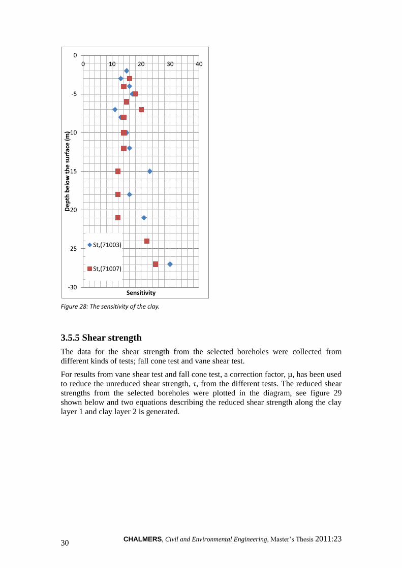
3.5.4 Sensitivity
The sensitivity of the clay has a value in range of 15 to 30. This shows that the clay is
sensitive, but not that much sensitive when compared with quick clay where the
sensitivity is over 50, see Figure 28.
-30
-25
-20
-15
-10
-5
0
0 20 40 60 80 100D
ep
th b
elo
w t
he
su
rfac
e (
m)
Liquid limit (%)
WL(%),71003
WL(%),FB41
WL(%),71007
CHALMERS, Civil and Environmental Engineering, Master’s Thesis 2011:23 30
Figure 28: The sensitivity of the clay.
3.5.5 Shear strength
The data for the shear strength from the selected boreholes were collected from
different kinds of tests; fall cone test and vane shear test.
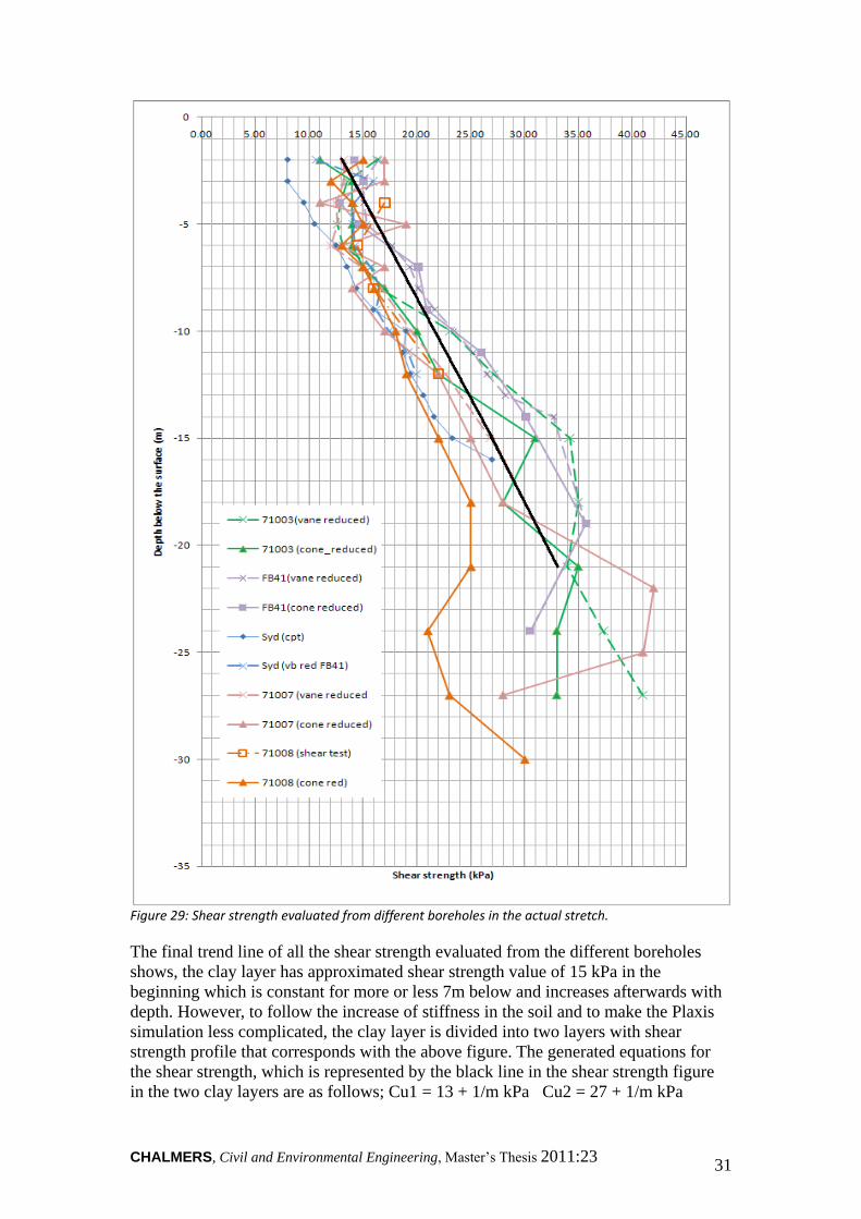
For results from vane shear test and fall cone test, a correction factor, µ, has been used
to reduce the unreduced shear strength, τ, from the different tests. The reduced shear
strengths from the selected boreholes were plotted in the diagram, see figure 29
shown below and two equations describing the reduced shear strength along the clay
layer 1 and clay layer 2 is generated.
-30
-25
-20
-15
-10
-5
0
0 10 20 30 40D
ep
th b
elo
w t
he
su
rfac
e (
m)
Sensitivity
St,(71003)
St,(71007)
CHALMERS, Civil and Environmental Engineering, Master’s Thesis 2011:23 31
Figure 29: Shear strength evaluated from different boreholes in the actual stretch.
The final trend line of all the shear strength evaluated from the different boreholes
shows, the clay layer has approximated shear strength value of 15 kPa in the
beginning which is constant for more or less 7m below and increases afterwards with
depth. However, to follow the increase of stiffness in the soil and to make the Plaxis
simulation less complicated, the clay layer is divided into two layers with shear
strength profile that corresponds with the above figure. The generated equations for
the shear strength, which is represented by the black line in the shear strength figure
in the two clay layers are as follows; Cu1 = 13 + 1/m kPa Cu2 = 27 + 1/m kPa
CHALMERS, Civil and Environmental Engineering, Master’s Thesis 2011:23 32
The formula shows that the shear strength is 13 kPa in the beginning of the first clay
layer and increases with 1 kPa each meter up to a depth of 13 meters where the second
clay layer begins. The second clay layer has initial shear strength of 27 kPa and
increases with 1 kPa each meter to the end of the clay layer. The equations describing
the shear strength properties of the clay profile are compared with the empirical
values according to Hansbo’s relation. The comparison shows that the reduced shear
strength values obtained from the tests are low, and therefore further investigations
shall be carried out in order to obtain a reasonable shear strength value.
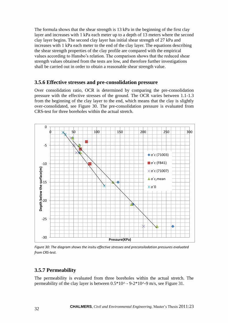
3.5.6 Effective stresses and pre-consolidation pressure
Over consolidation ratio, OCR is determined by comparing the pre-consolidation
pressure with the effective stresses of the ground. The OCR varies between 1.1-1.3
from the beginning of the clay layer to the end, which means that the clay is slightly
over-consolidated, see Figure 30. The pre-consolidation pressure is evaluated from
CRS-test for three boreholes within the actual stretch.
Figure 30: The diagram shows the insitu effective stresses and preconsilodation pressures evaluated
from CRS-test.
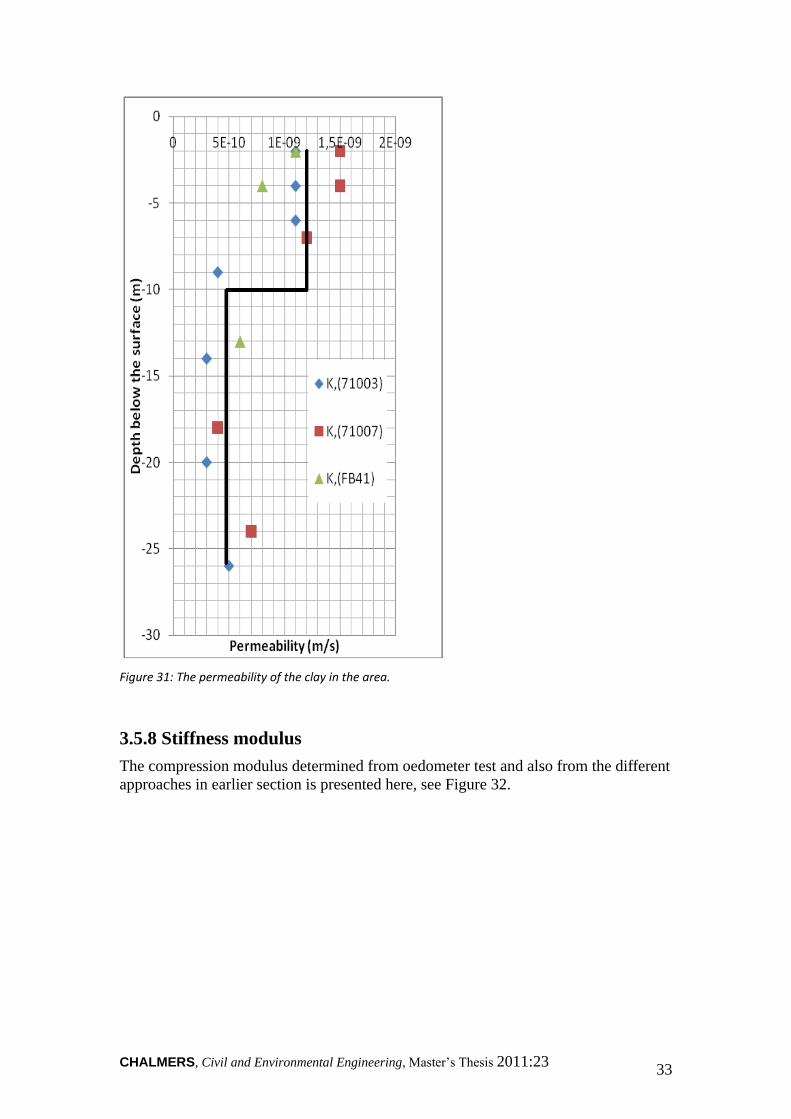
3.5.7 Permeability
The permeability is evaluated from three boreholes within the actual stretch. The
permeability of the clay layer is between 0.5*10^ - 9-2*10^-9 m/s, see Figure 31.
-30
-25
-20
-15
-10
-5
0
0 50 100 150 200 250 300
De
pth
be
low
th
e s
urf
ace
(m)
Pressure(KPa)
σ`c (71003)
σ`c (FB41)
σ`c (71007)
σ`c,mean
σ`0
CHALMERS, Civil and Environmental Engineering, Master’s Thesis 2011:23 33
Figure 31: The permeability of the clay in the area.
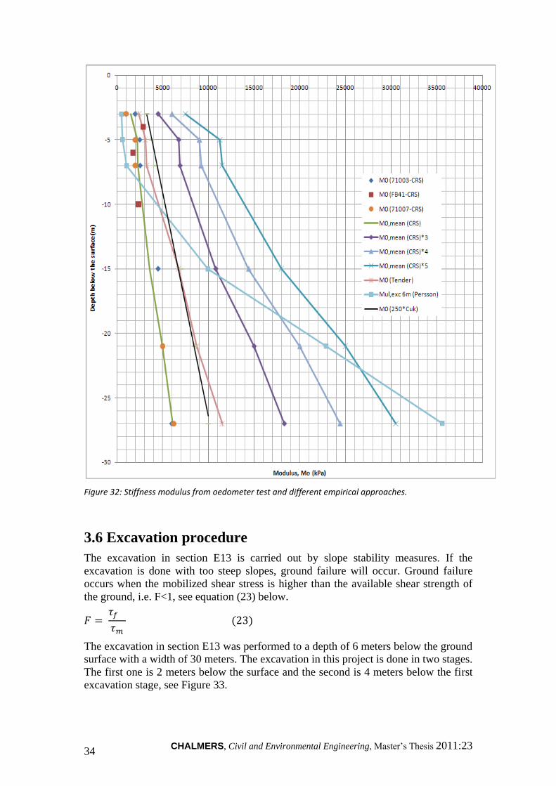
3.5.8 Stiffness modulus
The compression modulus determined from oedometer test and also from the different
approaches in earlier section is presented here, see Figure 32.
CHALMERS, Civil and Environmental Engineering, Master’s Thesis 2011:23 34
Figure 32: Stiffness modulus from oedometer test and different empirical approaches.
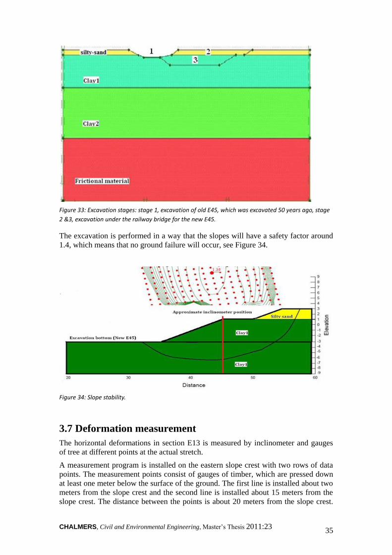
3.6 Excavation procedure
The excavation in section E13 is carried out by slope stability measures. If the
excavation is done with too steep slopes, ground failure will occur. Ground failure
occurs when the mobilized shear stress is higher than the available shear strength of
the ground, i.e. F<1, see equation (23) below.
( )
The excavation in section E13 was performed to a depth of 6 meters below the ground
surface with a width of 30 meters. The excavation in this project is done in two stages.
The first one is 2 meters below the surface and the second is 4 meters below the first
excavation stage, see Figure 33.
CHALMERS, Civil and Environmental Engineering, Master’s Thesis 2011:23 35
Figure 33: Excavation stages: stage 1, excavation of old E45, which was excavated 50 years ago, stage
2 &3, excavation under the railway bridge for the new E45.
The excavation is performed in a way that the slopes will have a safety factor around
1.4, which means that no ground failure will occur, see Figure 34.
Figure 34: Slope stability.
3.7 Deformation measurement
The horizontal deformations in section E13 is measured by inclinometer and gauges
of tree at different points at the actual stretch.
A measurement program is installed on the eastern slope crest with two rows of data
points. The measurement points consist of gauges of timber, which are pressed down
at least one meter below the surface of the ground. The first line is installed about two
meters from the slope crest and the second line is installed about 15 meters from the
slope crest. The distance between the points is about 20 meters from the slope crest.
CHALMERS, Civil and Environmental Engineering, Master’s Thesis 2011:23 36
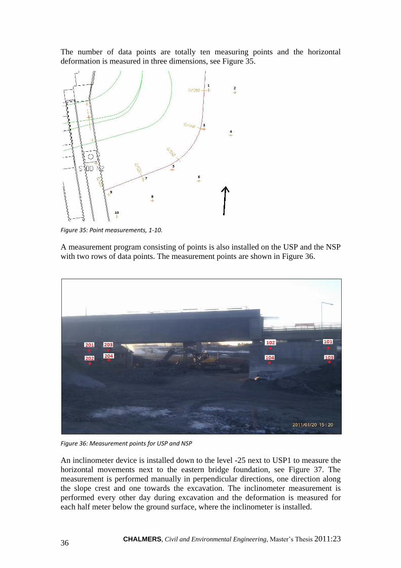
The number of data points are totally ten measuring points and the horizontal
deformation is measured in three dimensions, see Figure 35.
Figure 35: Point measurements, 1-10.
A measurement program consisting of points is also installed on the USP and the NSP
with two rows of data points. The measurement points are shown in Figure 36.
Figure 36: Measurement points for USP and NSP
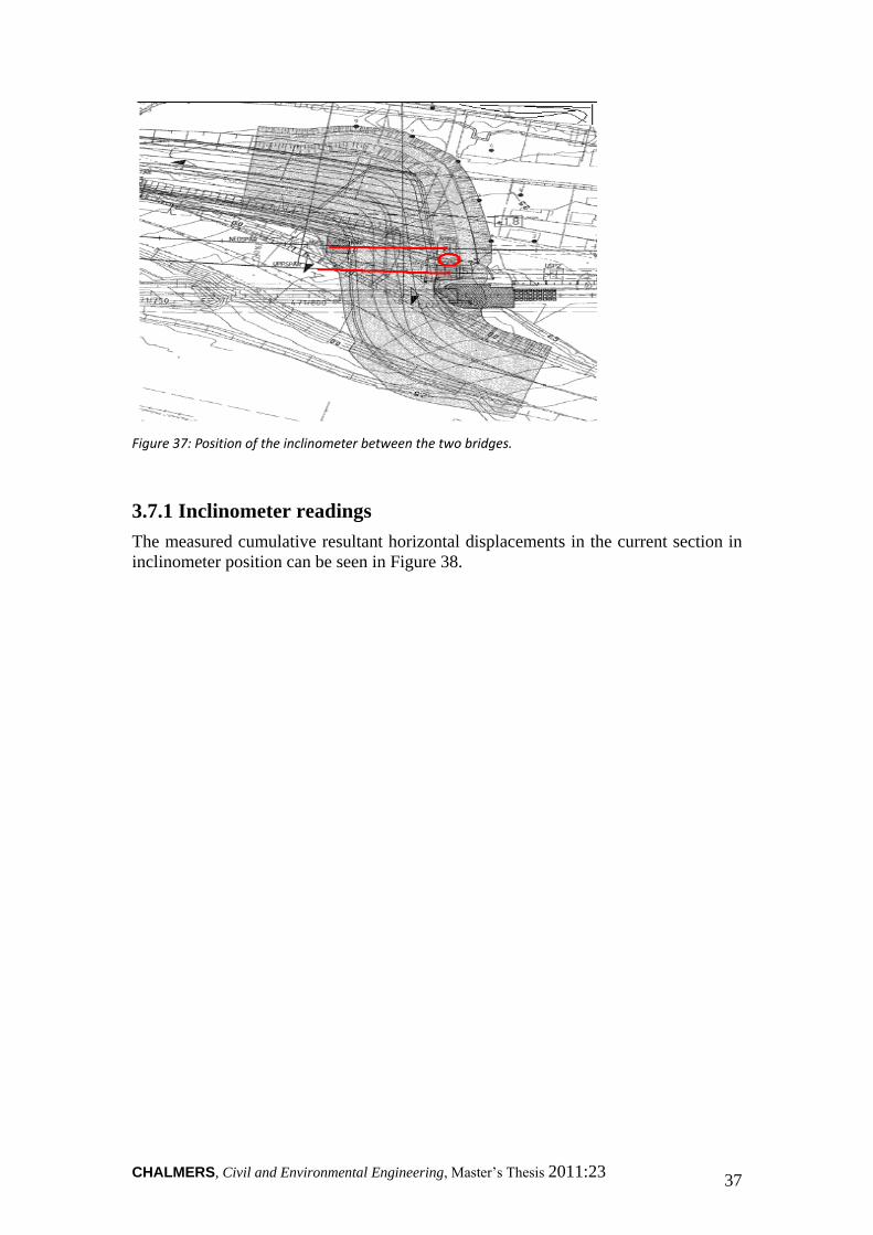
An inclinometer device is installed down to the level -25 next to USP1 to measure the
horizontal movements next to the eastern bridge foundation, see Figure 37. The
measurement is performed manually in perpendicular directions, one direction along
the slope crest and one towards the excavation. The inclinometer measurement is
performed every other day during excavation and the deformation is measured for
each half meter below the ground surface, where the inclinometer is installed.
CHALMERS, Civil and Environmental Engineering, Master’s Thesis 2011:23 37
Figure 37: Position of the inclinometer between the two bridges.
3.7.1 Inclinometer readings
The measured cumulative resultant horizontal displacements in the current section in
inclinometer position can be seen in Figure 38.

CHALMERS, Civil and Environmental Engineering, Master’s Thesis 2011:23 38
Figure 38: Cumulative resultant horizontal deformations by inclinometer device.
The above presented diagram shows that there is no horizontal movement below a
depth of 27 meters down. As it can be seen the maximum horizontal deformation is
occurring around a depth of 9 meters below the ground surface. The horizontal
movement curve is showing that the deformation is decreasing from the depth of 9
meters to the upper level of the clay. This decrease in value is due to the situation
around the bridge foundation, which is discussed more in Outputs chapter.
3.7.2 Gauges readings
As mentioned in section 3.7, a study of the horizontal movement at the surface of the
slope crest has been performed. The measurement consists of points that measure the
movement in x, y and z directions.
-30
-25
-20
-15
-10
-5
0
0 10 20 30 40 50 60
De
pth
be
low
th
e g
rou
nd
su
rfac
e (
m)
Cumulative horizontal deformation (mm)
Inclinometer
CHALMERS, Civil and Environmental Engineering, Master’s Thesis 2011:23 39
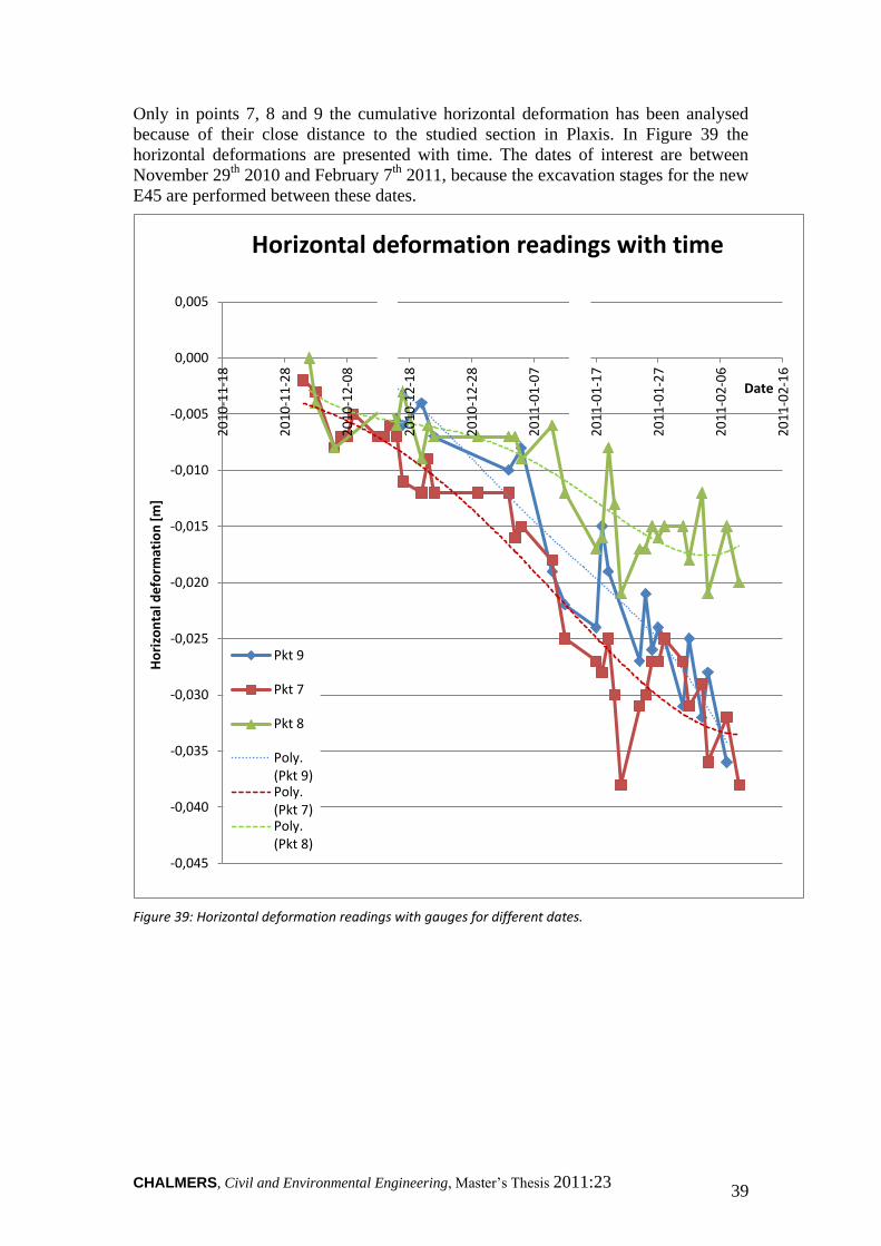
Only in points 7, 8 and 9 the cumulative horizontal deformation has been analysed
because of their close distance to the studied section in Plaxis. In Figure 39 the
horizontal deformations are presented with time. The dates of interest are between
November 29th
2010 and February 7th
2011, because the excavation stages for the new
E45 are performed between these dates.
Figure 39: Horizontal deformation readings with gauges for different dates.
-0,045
-0,040
-0,035
-0,030
-0,025
-0,020
-0,015
-0,010
-0,005
0,000
0,005
20
10
-11
-18
20
10
-11
-28
20
10
-12
-08
20
10
-12
-18
20
10
-12
-28
20
11
-01
-07
20
11
-01
-17
20
11
-01
-27
20
11
-02
-06
20
11
-02
-16
Ho
rizo
nta
l de
form
atio
n [
m]
Date
Horizontal deformation readings with time
Pkt 9
Pkt 7
Pkt 8
Poly.(Pkt 9)Poly.(Pkt 7)Poly.(Pkt 8)
CHALMERS, Civil and Environmental Engineering, Master’s Thesis 2011:23 40
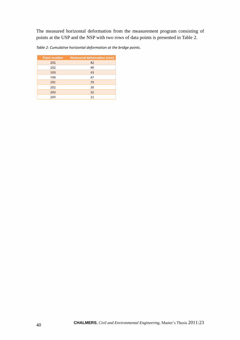
The measured horizontal deformation from the measurement program consisting of
points at the USP and the NSP with two rows of data points is presented in Table 2.
Table 2: Cumulative horizontal deformation at the bridge points.
CHALMERS, Civil and Environmental Engineering, Master’s Thesis 2011:23 41
4. Plaxis analysis
Once all the relevant input data from field and laboratory tests, and mathematical
hand and empirical calculations are collected, the Plaxis deformation analysis
proceeds. As mentioned in the theory part, the Plaxis analysis includes the input,
calculation and output phases. However, in this section only the first two phases are
discussed. The later phase is discussed in the result section together with the field
measurements, the inclinometer readings and surface point measurements.
4.1 Input phase
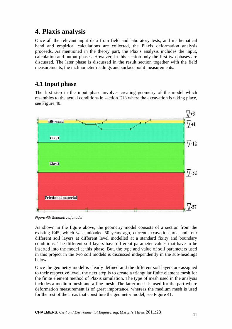
The first step in the input phase involves creating geometry of the model which
resembles to the actual conditions in section E13 where the excavation is taking place,
see Figure 40.
Figure 40: Geometry of model
As shown in the figure above, the geometry model consists of a section from the
existing E45, which was unloaded 50 years ago, current excavation area and four
different soil layers at different level modelled at a standard fixity and boundary
conditions. The different soil layers have different parameter values that have to be
inserted into the model at this phase. But, the type and value of soil parameters used
in this project in the two soil models is discussed independently in the sub-headings
below.
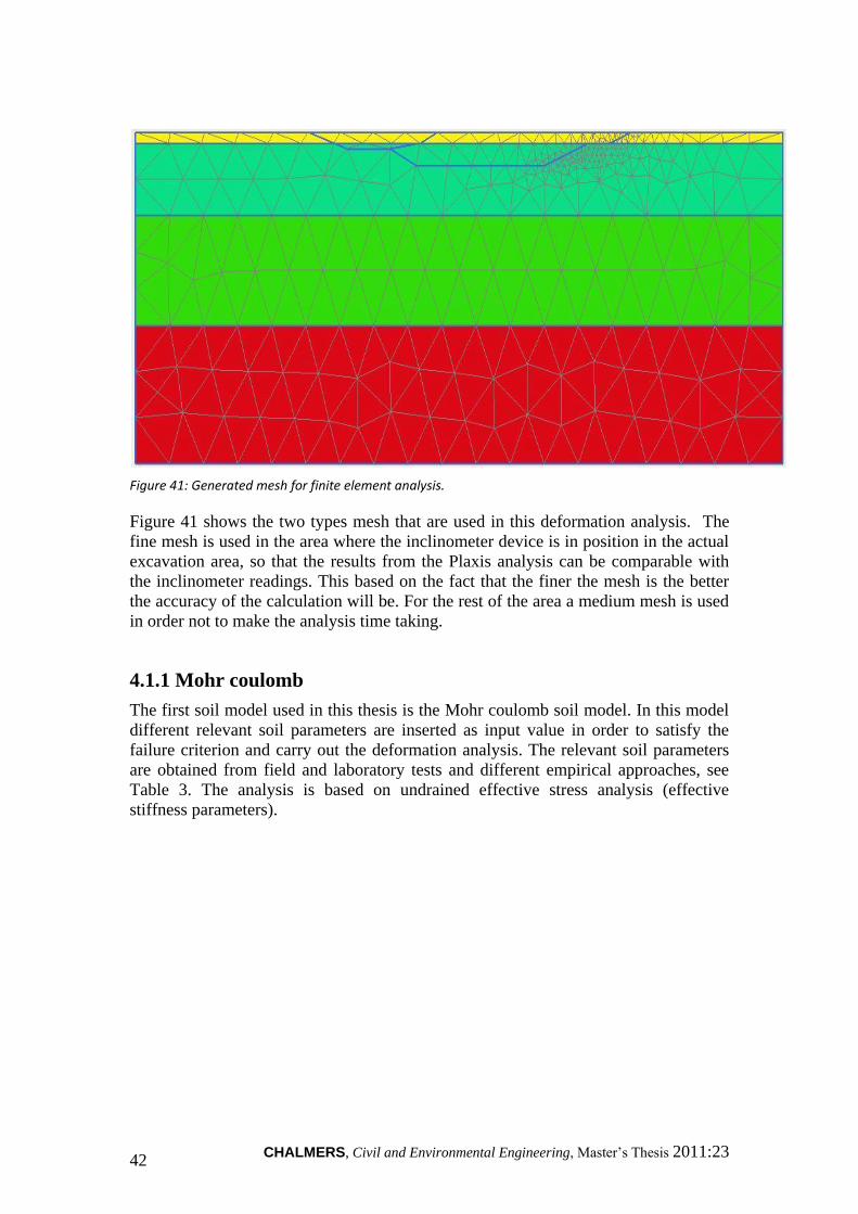
Once the geometry model is clearly defined and the different soil layers are assigned
to their respective level, the next step is to create a triangular finite element mesh for
the finite element method of Plaxis simulation. The type of mesh used in the analysis
includes a medium mesh and a fine mesh. The latter mesh is used for the part where
deformation measurement is of great importance, whereas the medium mesh is used
for the rest of the areas that constitute the geometry model, see Figure 41.
CHALMERS, Civil and Environmental Engineering, Master’s Thesis 2011:23 42
Figure 41: Generated mesh for finite element analysis.
Figure 41 shows the two types mesh that are used in this deformation analysis. The
fine mesh is used in the area where the inclinometer device is in position in the actual
excavation area, so that the results from the Plaxis analysis can be comparable with
the inclinometer readings. This based on the fact that the finer the mesh is the better
the accuracy of the calculation will be. For the rest of the area a medium mesh is used
in order not to make the analysis time taking.
4.1.1 Mohr coulomb
The first soil model used in this thesis is the Mohr coulomb soil model. In this model
different relevant soil parameters are inserted as input value in order to satisfy the
failure criterion and carry out the deformation analysis. The relevant soil parameters
are obtained from field and laboratory tests and different empirical approaches, see
Table 3. The analysis is based on undrained effective stress analysis (effective
stiffness parameters).

CHALMERS, Civil and Environmental Engineering, Master’s Thesis 2011:23 43
Table 3: Input parameters for Mohr coulomb model
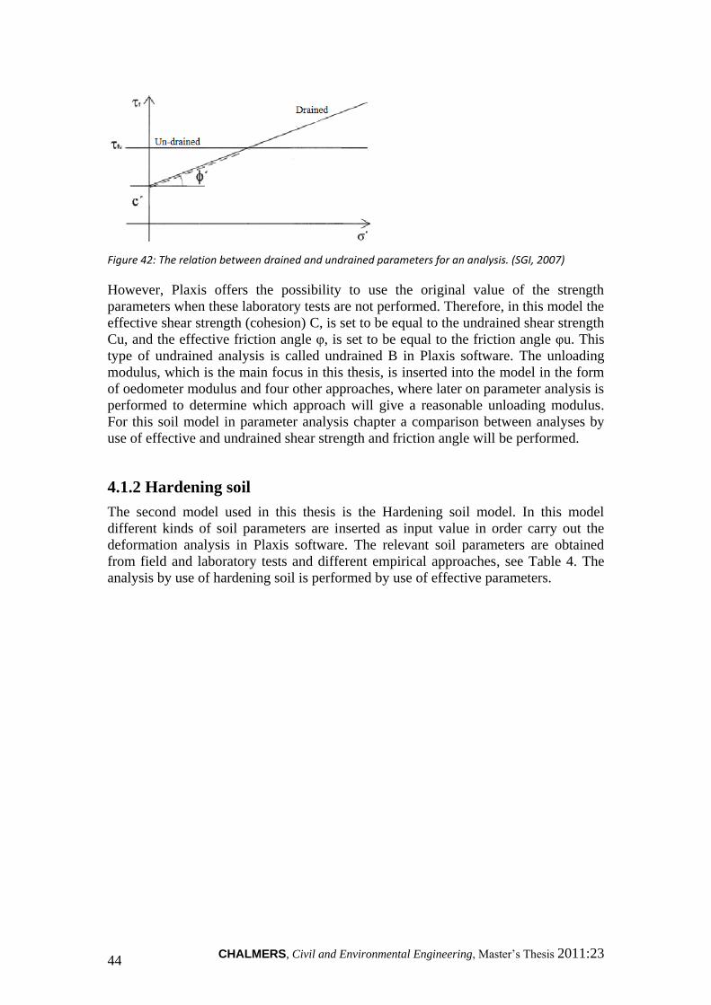
Even though the analysis is based on undrained effective stress analysis, only young’s
modulus and poisson’s ratio are used as effective parameters. This is due to not being
able to get effective parameters for the other strength parameters without performing
laboratory tests. Using effective values of shear strength for higher effective stresses
will lead to a high shear strength compared to the undrained shear strength obtained
by field and laboratory tests. The use of effective shear strength for lower effective
stress states will lead to a low shear strength compared to the values of undrained
shear strength obtained by field and laboratory tests see Figure 42.
CHALMERS, Civil and Environmental Engineering, Master’s Thesis 2011:23 44
Figure 42: The relation between drained and undrained parameters for an analysis. (SGI, 2007)
However, Plaxis offers the possibility to use the original value of the strength
parameters when these laboratory tests are not performed. Therefore, in this model the
effective shear strength (cohesion) C, is set to be equal to the undrained shear strength
Cu, and the effective friction angle υ, is set to be equal to the friction angle υu. This
type of undrained analysis is called undrained B in Plaxis software. The unloading
modulus, which is the main focus in this thesis, is inserted into the model in the form
of oedometer modulus and four other approaches, where later on parameter analysis is
performed to determine which approach will give a reasonable unloading modulus.
For this soil model in parameter analysis chapter a comparison between analyses by
use of effective and undrained shear strength and friction angle will be performed.
4.1.2 Hardening soil
The second model used in this thesis is the Hardening soil model. In this model
different kinds of soil parameters are inserted as input value in order carry out the
deformation analysis in Plaxis software. The relevant soil parameters are obtained
from field and laboratory tests and different empirical approaches, see Table 4. The
analysis by use of hardening soil is performed by use of effective parameters.
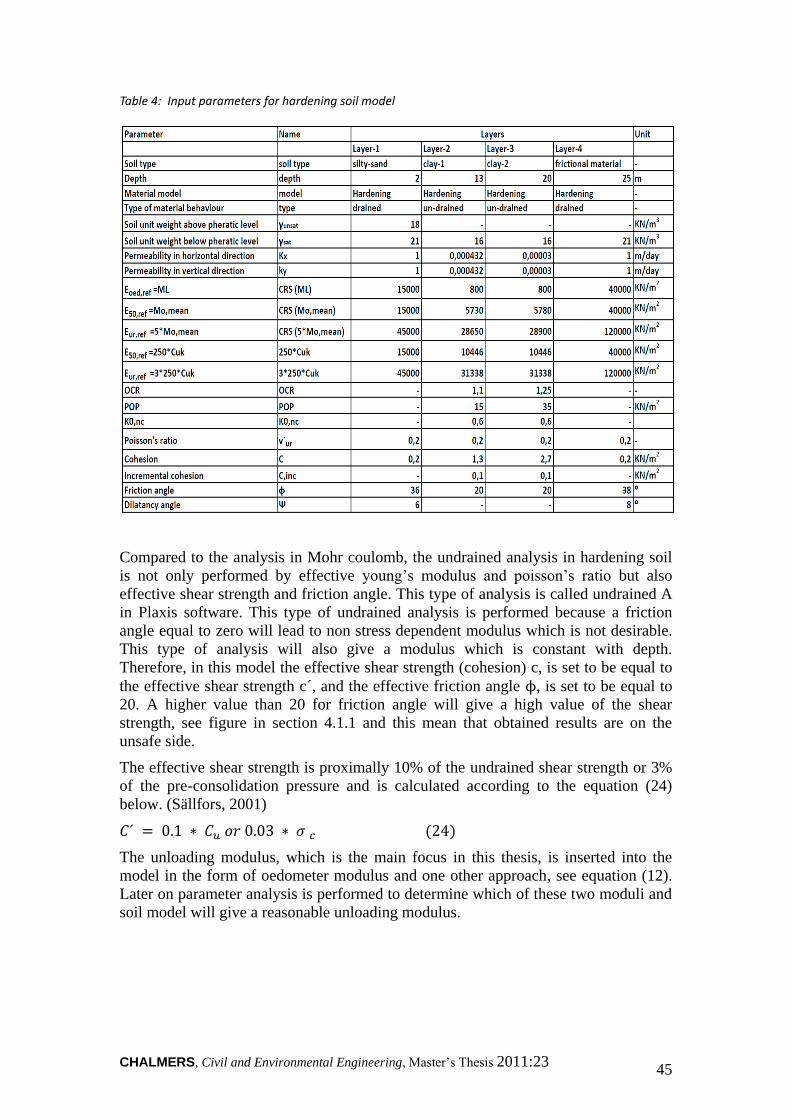
CHALMERS, Civil and Environmental Engineering, Master’s Thesis 2011:23 45
Table 4: Input parameters for hardening soil model
Compared to the analysis in Mohr coulomb, the undrained analysis in hardening soil
is not only performed by effective young’s modulus and poisson’s ratio but also
effective shear strength and friction angle. This type of analysis is called undrained A
in Plaxis software. This type of undrained analysis is performed because a friction
angle equal to zero will lead to non stress dependent modulus which is not desirable.
This type of analysis will also give a modulus which is constant with depth.
Therefore, in this model the effective shear strength (cohesion) c, is set to be equal to
the effective shear strength c´, and the effective friction angle ϕ, is set to be equal to
20. A higher value than 20 for friction angle will give a high value of the shear
strength, see figure in section 4.1.1 and this mean that obtained results are on the
unsafe side.
The effective shear strength is proximally 10% of the undrained shear strength or 3%
of the pre-consolidation pressure and is calculated according to the equation (24)
below. (Sällfors, 2001)
( )
The unloading modulus, which is the main focus in this thesis, is inserted into the
model in the form of oedometer modulus and one other approach, see equation (12).
Later on parameter analysis is performed to determine which of these two moduli and
soil model will give a reasonable unloading modulus.
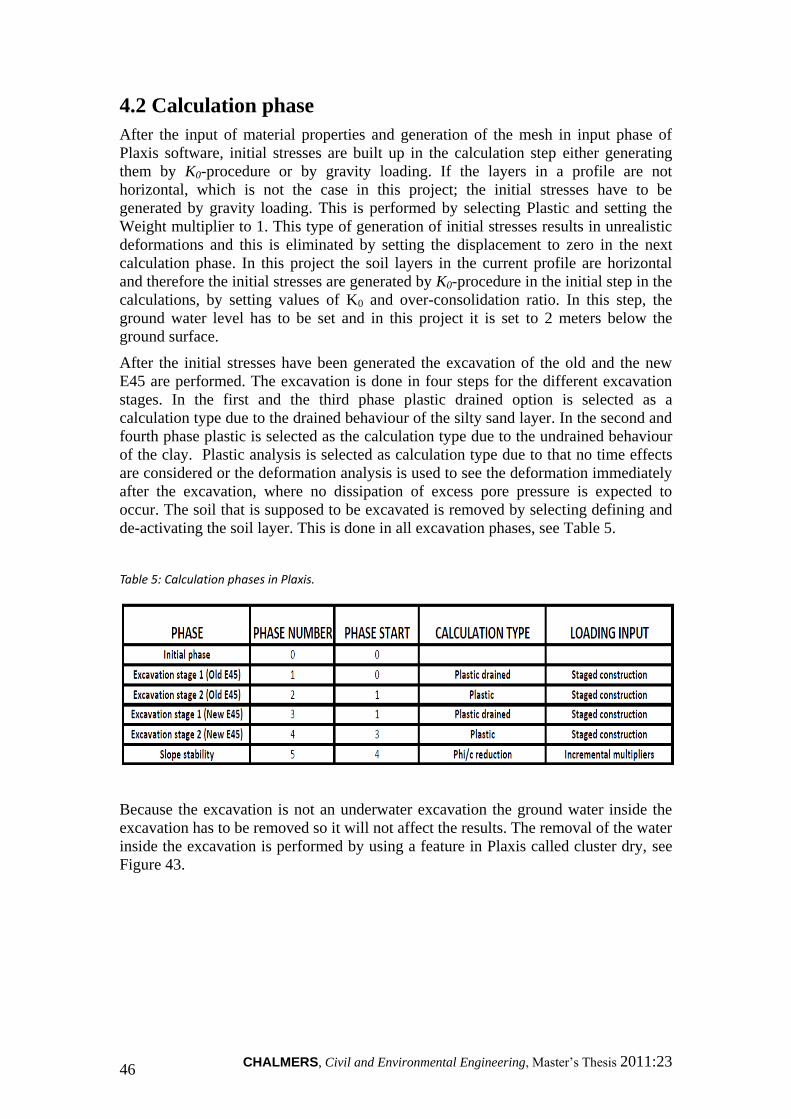
CHALMERS, Civil and Environmental Engineering, Master’s Thesis 2011:23 46
4.2 Calculation phase
After the input of material properties and generation of the mesh in input phase of
Plaxis software, initial stresses are built up in the calculation step either generating
them by K0-procedure or by gravity loading. If the layers in a profile are not
horizontal, which is not the case in this project; the initial stresses have to be
generated by gravity loading. This is performed by selecting Plastic and setting the
Weight multiplier to 1. This type of generation of initial stresses results in unrealistic
deformations and this is eliminated by setting the displacement to zero in the next
calculation phase. In this project the soil layers in the current profile are horizontal
and therefore the initial stresses are generated by K0-procedure in the initial step in the
calculations, by setting values of K0 and over-consolidation ratio. In this step, the
ground water level has to be set and in this project it is set to 2 meters below the
ground surface.
After the initial stresses have been generated the excavation of the old and the new
E45 are performed. The excavation is done in four steps for the different excavation
stages. In the first and the third phase plastic drained option is selected as a
calculation type due to the drained behaviour of the silty sand layer. In the second and
fourth phase plastic is selected as the calculation type due to the undrained behaviour
of the clay. Plastic analysis is selected as calculation type due to that no time effects
are considered or the deformation analysis is used to see the deformation immediately
after the excavation, where no dissipation of excess pore pressure is expected to
occur. The soil that is supposed to be excavated is removed by selecting defining and
de-activating the soil layer. This is done in all excavation phases, see Table 5.
Table 5: Calculation phases in Plaxis.
Because the excavation is not an underwater excavation the ground water inside the
excavation has to be removed so it will not affect the results. The removal of the water
inside the excavation is performed by using a feature in Plaxis called cluster dry, see
Figure 43.

CHALMERS, Civil and Environmental Engineering, Master’s Thesis 2011:23 47
Figure 43: Dry excavation in Plaxis analysis.
In the fifth phase, see table above, the slope stability analysis is performed by an
option called phi/c reduction. The idea of this calculation type is to reduce the c and ϕ until the soil collapses and then the values of cohesion and friction angle are recorded.
These values give at which values the soil fails and are compared to the actual shear
strength and friction angle. By the comparison a safety factor F for the slope failure is
obtained, see equation (25) below.
( )
After the calculation step, the deformations and the stability of the slope can be
evaluated in the outputs and are presented in the next chapter together with the results
from field measurements.
4.3 Outputs
Among the different output results that can be obtained from Plaxis, such as
deformations of geotechnical and structural elements, slope stability, steady pore-
water pressure and development of excessive pore pressures and consolidation
parameters, this thesis is concerned with horizontal displacements due to excavation.
Additionally, since the excavation has taken place in short period time plastic analysis
is only performed rather than consolidation analysis and all results regarding
consolidation process obtained from the Plaxis simulation are therefore considered to
be not relevant to this project.
The horizontal phase displacement readings are taken in form of cross section in
points where the inclinometer and point measurement devices are installed in the
actual excavation area, see Figure 44.
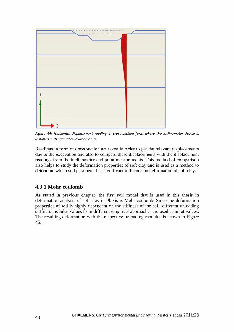
CHALMERS, Civil and Environmental Engineering, Master’s Thesis 2011:23 48
Figure 44: Horizontal displacement reading in cross section form where the inclinometer device is
installed in the actual excavation area.
Readings in form of cross section are taken in order to get the relevant displacements
due to the excavation and also to compare these displacements with the displacement
readings from the inclinometer and point measurements. This method of comparison
also helps to study the deformation properties of soft clay and is used as a method to
determine which soil parameter has significant influence on deformation of soft clay.
4.3.1 Mohr coulomb
As stated in previous chapter, the first soil model that is used in this thesis in
deformation analysis of soft clay in Plaxis is Mohr coulomb. Since the deformation
properties of soil is highly dependent on the stiffness of the soil, different unloading
stiffness modulus values from different empirical approaches are used as input values.
The resulting deformation with the respective unloading modulus is shown in Figure
45.
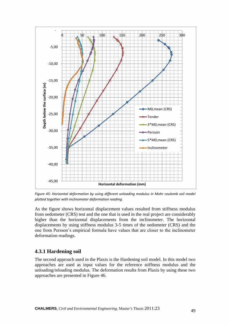
CHALMERS, Civil and Environmental Engineering, Master’s Thesis 2011:23 49
Figure 45: Horizontal deformation by using different unloading modulus in Mohr coulomb soil model
plotted together with inclinometer deformation reading.
As the figure shows horizontal displacement values resulted from stiffness modulus
from oedometer (CRS) test and the one that is used in the real project are considerably
higher than the horizontal displacements from the inclinometer. The horizontal
displacements by using stiffness modulus 3-5 times of the oedometer (CRS) and the
one from Persson’s empirical formula have values that are closer to the inclinometer
deformation readings.
4.3.1 Hardening soil
The second approach used in the Plaxis is the Hardening soil model. In this model two
approaches are used as input values for the reference stiffness modulus and the
unloading/reloading modulus. The deformation results from Plaxis by using these two
approaches are presented in Figure 46.
-45,00
-40,00
-35,00
-30,00
-25,00
-20,00
-15,00
-10,00
-5,00
-
0 50 100 150 200 250 300
De
pth
be
low
th
e s
urf
ace
(m
)
Horizontal deformation (mm)
M0,mean (CRS)
Tender
3*M0,mean (CRS)
Persson
5*M0,mean (CRS)
Inclinometer
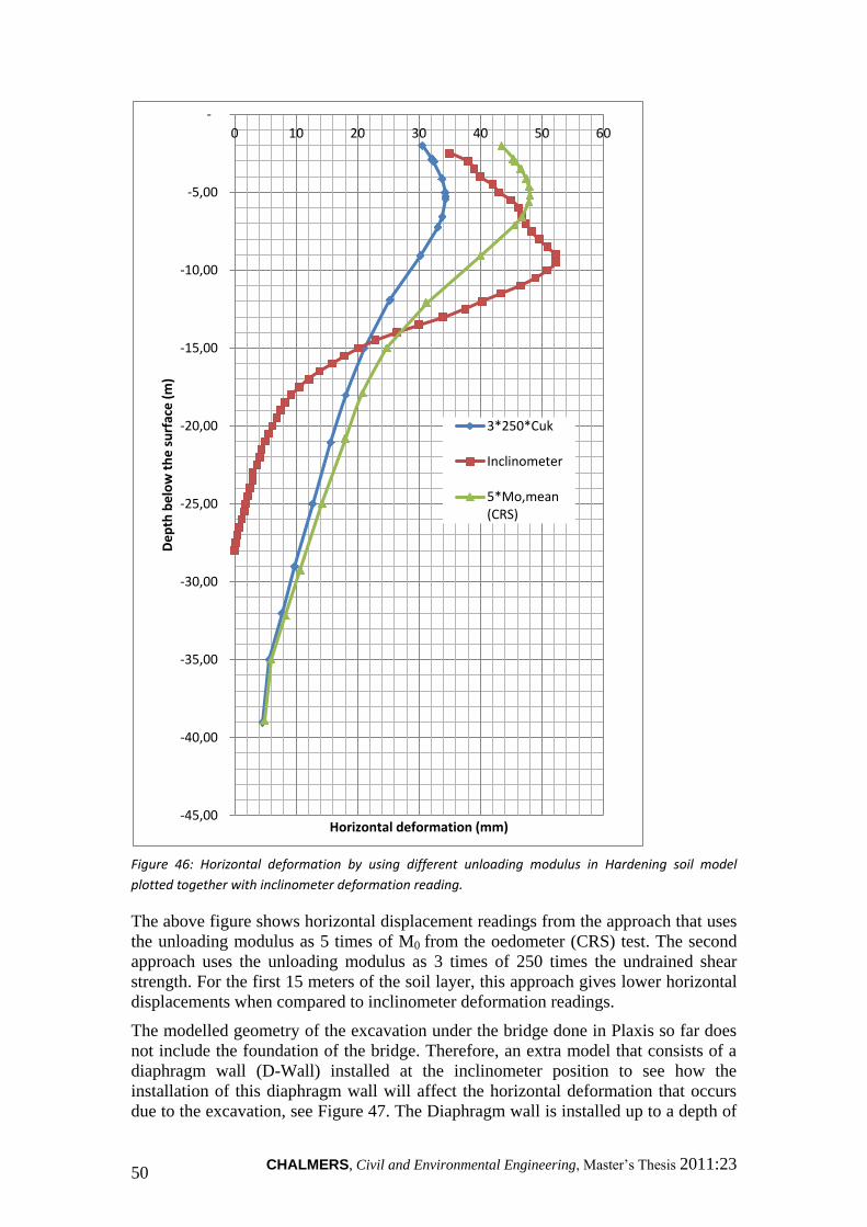
CHALMERS, Civil and Environmental Engineering, Master’s Thesis 2011:23 50
Figure 46: Horizontal deformation by using different unloading modulus in Hardening soil model
plotted together with inclinometer deformation reading.
The above figure shows horizontal displacement readings from the approach that uses
the unloading modulus as 5 times of M0 from the oedometer (CRS) test. The second
approach uses the unloading modulus as 3 times of 250 times the undrained shear
strength. For the first 15 meters of the soil layer, this approach gives lower horizontal
displacements when compared to inclinometer deformation readings.
The modelled geometry of the excavation under the bridge done in Plaxis so far does
not include the foundation of the bridge. Therefore, an extra model that consists of a
diaphragm wall (D-Wall) installed at the inclinometer position to see how the
installation of this diaphragm wall will affect the horizontal deformation that occurs
due to the excavation, see Figure 47. The Diaphragm wall is installed up to a depth of
-45,00
-40,00
-35,00
-30,00
-25,00
-20,00
-15,00
-10,00
-5,00
-
0 10 20 30 40 50 60
De
pth
be
low
th
e s
urf
ace
(m
)
Horizontal deformation (mm)
3*250*Cuk
Inclinometer
5*Mo,mean(CRS)
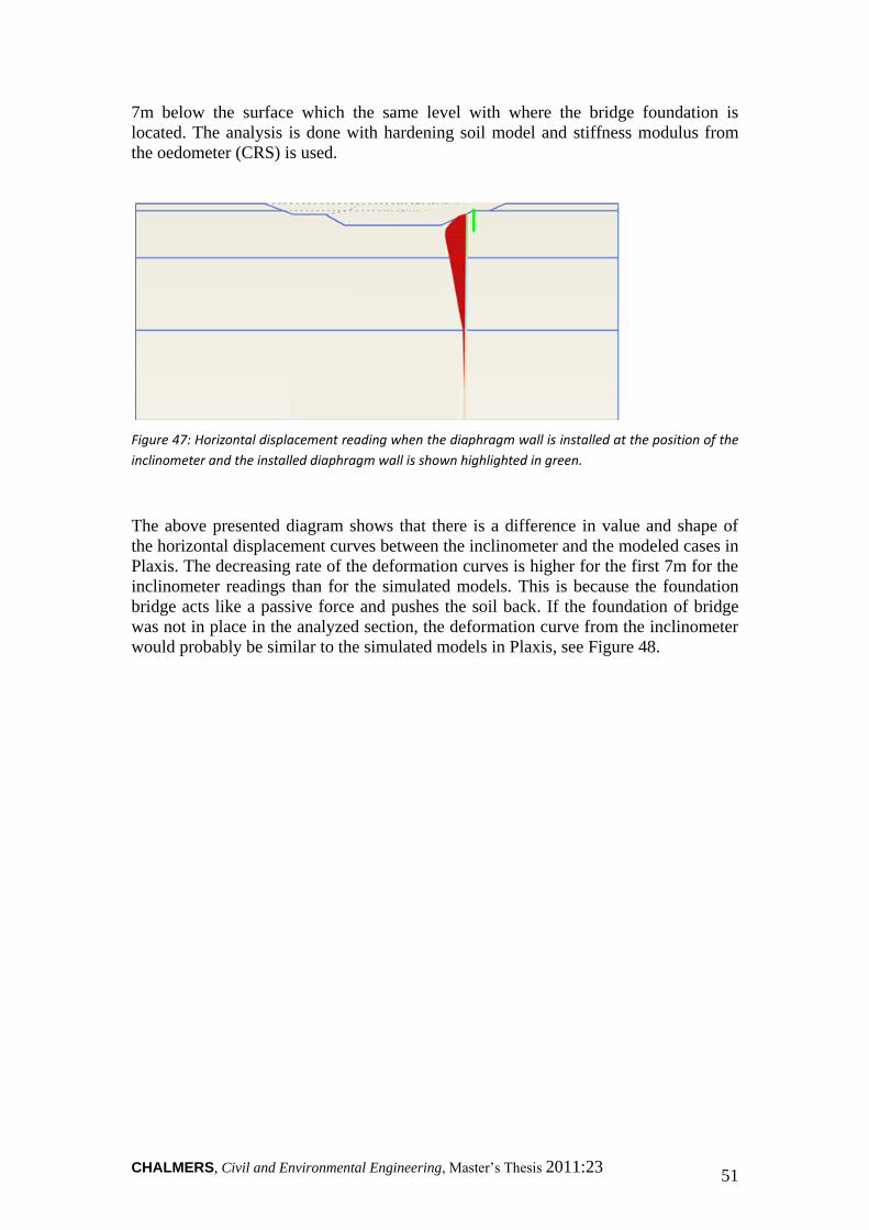
CHALMERS, Civil and Environmental Engineering, Master’s Thesis 2011:23 51
7m below the surface which the same level with where the bridge foundation is
located. The analysis is done with hardening soil model and stiffness modulus from
the oedometer (CRS) is used.
Figure 47: Horizontal displacement reading when the diaphragm wall is installed at the position of the
inclinometer and the installed diaphragm wall is shown highlighted in green.
The above presented diagram shows that there is a difference in value and shape of
the horizontal displacement curves between the inclinometer and the modeled cases in
Plaxis. The decreasing rate of the deformation curves is higher for the first 7m for the
inclinometer readings than for the simulated models. This is because the foundation
bridge acts like a passive force and pushes the soil back. If the foundation of bridge
was not in place in the analyzed section, the deformation curve from the inclinometer
would probably be similar to the simulated models in Plaxis, see Figure 48.
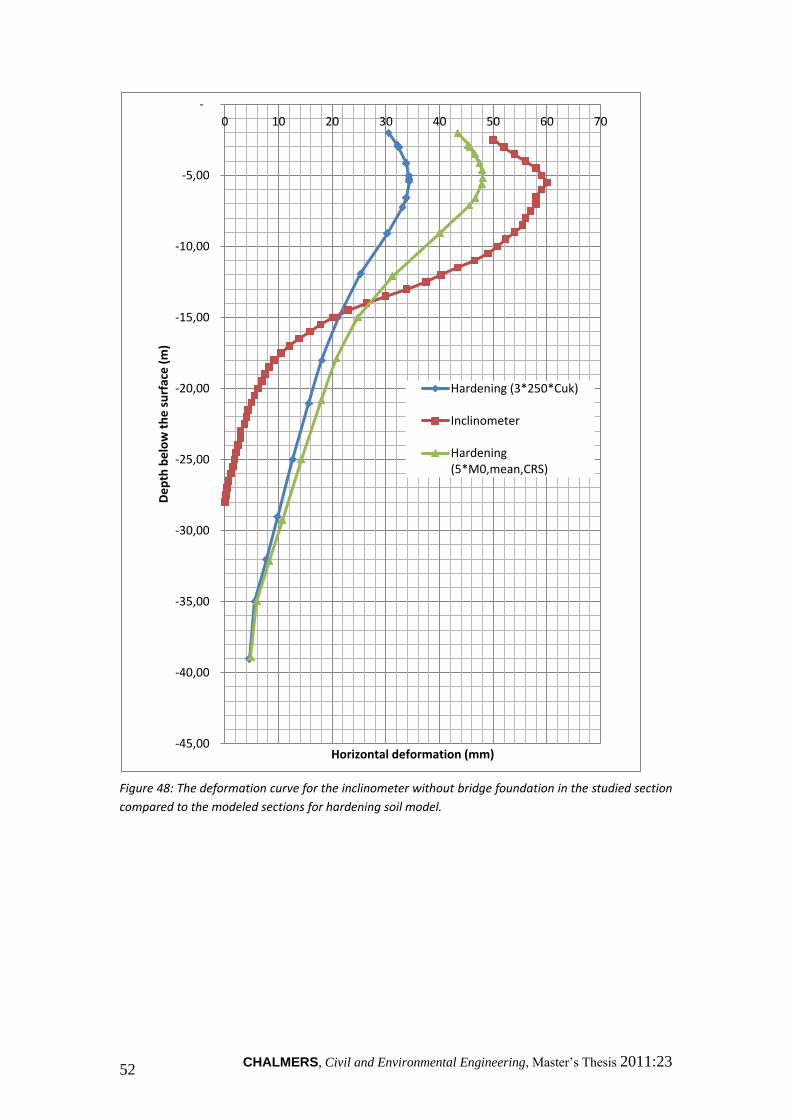
CHALMERS, Civil and Environmental Engineering, Master’s Thesis 2011:23 52
Figure 48: The deformation curve for the inclinometer without bridge foundation in the studied section
compared to the modeled sections for hardening soil model.
-45,00
-40,00
-35,00
-30,00
-25,00
-20,00
-15,00
-10,00
-5,00
-
0 10 20 30 40 50 60 70
De
pth
be
low
th
e s
urf
ace
(m
)
Horizontal deformation (mm)
Hardening (3*250*Cuk)
Inclinometer
Hardening(5*M0,mean,CRS)

CHALMERS, Civil and Environmental Engineering, Master’s Thesis 2011:23 53
5. Result comparison
In this chapter a comparison is carried out between horizontal deformations obtained
from the inclinometer device and all the simulated models in Plaxis. In Figure 49 the
horizontal deformation comparison between the soil models and the inclinometer
device throughout the soil layer can be seen.
Figure 49: Horizontal deformation by using different unloading modulus in Mohr coulomb soil model
(the five first names in the diagram) and Hardening soil model (the last two names in the diagram)
plotted together with inclinometer deformation reading
Because of the impact of the foundation there is no possibility to make a comparison
between the inclinometer readings and the simulations performed in Plaxis for the
first 6-8 meters of the soil layer. Therefore the comparison is performed where the
inclinometer gives largest horizontal displacements, which is around a depth of 9
meters below the ground surface. In Table 6 the horizontal deformations from the
-45,00
-40,00
-35,00
-30,00
-25,00
-20,00
-15,00
-10,00
-5,00
-
0 50 100 150 200 250 300
De
pth
be
low
th
e s
urf
ace
(m
)
Horizontal deformation (mm)
M0,mean (CRS)
Tender
3*M0,mean (CRS)
Persson
5*M0,mean (CRS)
Inclinometer
3*250*Cuk
5*Mo,mean (CRS)
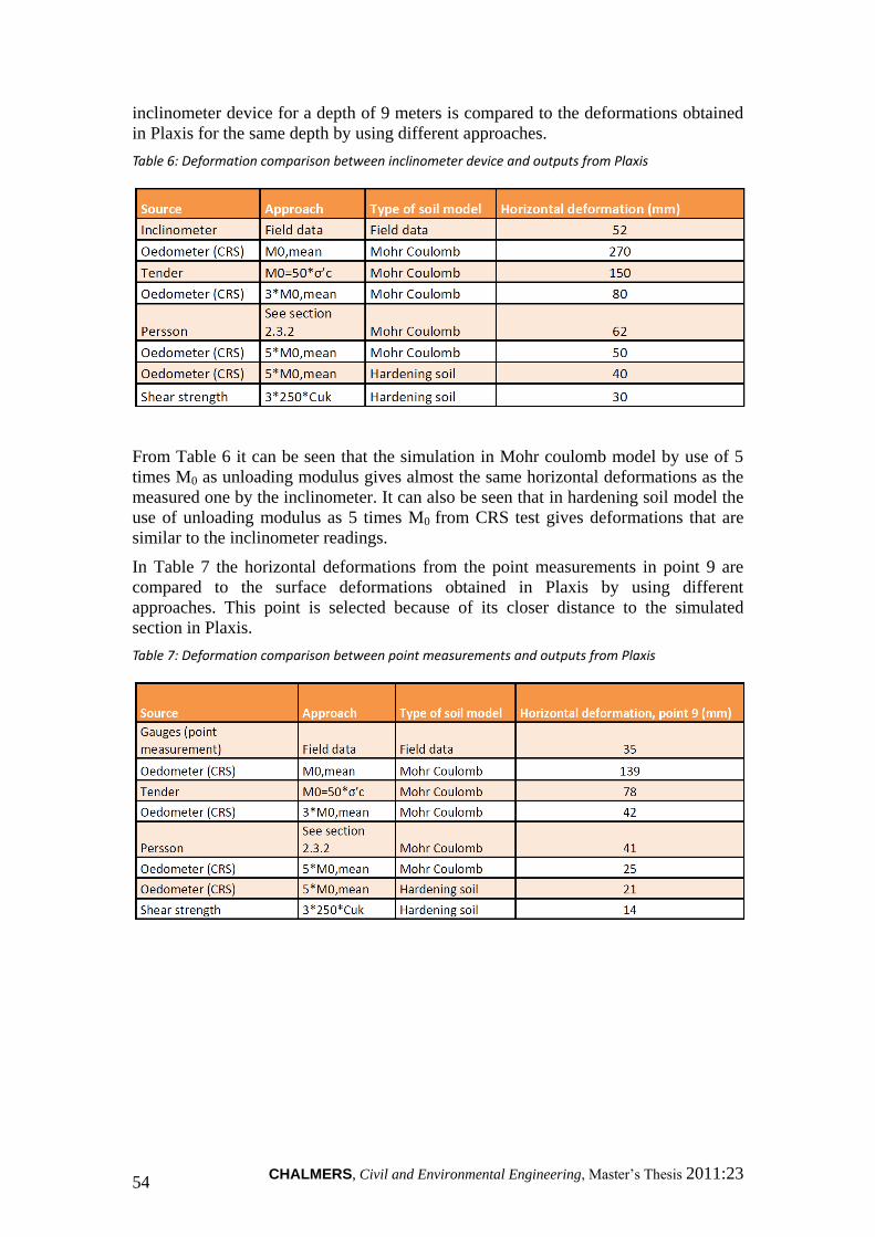
CHALMERS, Civil and Environmental Engineering, Master’s Thesis 2011:23 54
inclinometer device for a depth of 9 meters is compared to the deformations obtained
in Plaxis for the same depth by using different approaches.
Table 6: Deformation comparison between inclinometer device and outputs from Plaxis
From Table 6 it can be seen that the simulation in Mohr coulomb model by use of 5
times M0 as unloading modulus gives almost the same horizontal deformations as the
measured one by the inclinometer. It can also be seen that in hardening soil model the
use of unloading modulus as 5 times M0 from CRS test gives deformations that are
similar to the inclinometer readings.
In Table 7 the horizontal deformations from the point measurements in point 9 are
compared to the surface deformations obtained in Plaxis by using different
approaches. This point is selected because of its closer distance to the simulated
section in Plaxis.
Table 7: Deformation comparison between point measurements and outputs from Plaxis
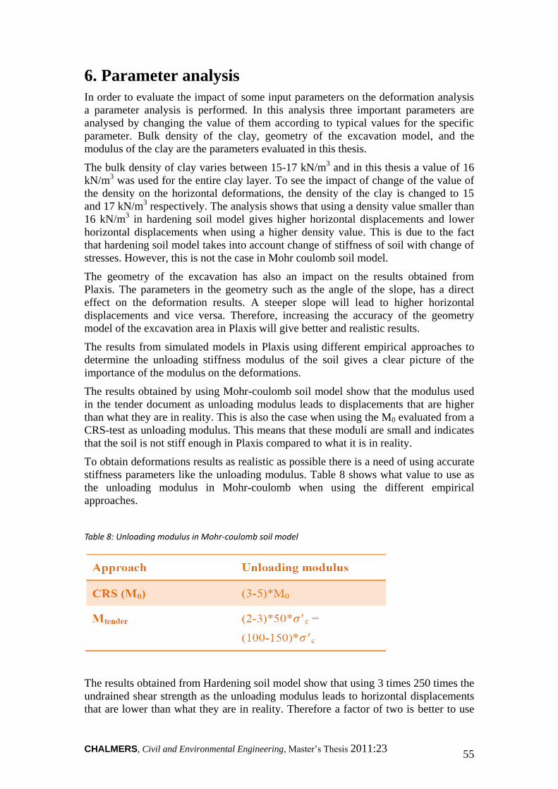
CHALMERS, Civil and Environmental Engineering, Master’s Thesis 2011:23 55
6. Parameter analysis
In order to evaluate the impact of some input parameters on the deformation analysis
a parameter analysis is performed. In this analysis three important parameters are
analysed by changing the value of them according to typical values for the specific
parameter. Bulk density of the clay, geometry of the excavation model, and the
modulus of the clay are the parameters evaluated in this thesis.
The bulk density of clay varies between 15-17 kN/m3 and in this thesis a value of 16
kN/m3 was used for the entire clay layer. To see the impact of change of the value of
the density on the horizontal deformations, the density of the clay is changed to 15
and 17 kN/m3 respectively. The analysis shows that using a density value smaller than
16 kN/m3 in hardening soil model gives higher horizontal displacements and lower
horizontal displacements when using a higher density value. This is due to the fact
that hardening soil model takes into account change of stiffness of soil with change of
stresses. However, this is not the case in Mohr coulomb soil model.
The geometry of the excavation has also an impact on the results obtained from
Plaxis. The parameters in the geometry such as the angle of the slope, has a direct
effect on the deformation results. A steeper slope will lead to higher horizontal
displacements and vice versa. Therefore, increasing the accuracy of the geometry
model of the excavation area in Plaxis will give better and realistic results.
The results from simulated models in Plaxis using different empirical approaches to
determine the unloading stiffness modulus of the soil gives a clear picture of the
importance of the modulus on the deformations.
The results obtained by using Mohr-coulomb soil model show that the modulus used
in the tender document as unloading modulus leads to displacements that are higher
than what they are in reality. This is also the case when using the M0 evaluated from a
CRS-test as unloading modulus. This means that these moduli are small and indicates
that the soil is not stiff enough in Plaxis compared to what it is in reality.
To obtain deformations results as realistic as possible there is a need of using accurate
stiffness parameters like the unloading modulus. Table 8 shows what value to use as
the unloading modulus in Mohr-coulomb when using the different empirical
approaches.
Table 8: Unloading modulus in Mohr-coulomb soil model
The results obtained from Hardening soil model show that using 3 times 250 times the
undrained shear strength as the unloading modulus leads to horizontal displacements
that are lower than what they are in reality. Therefore a factor of two is better to use
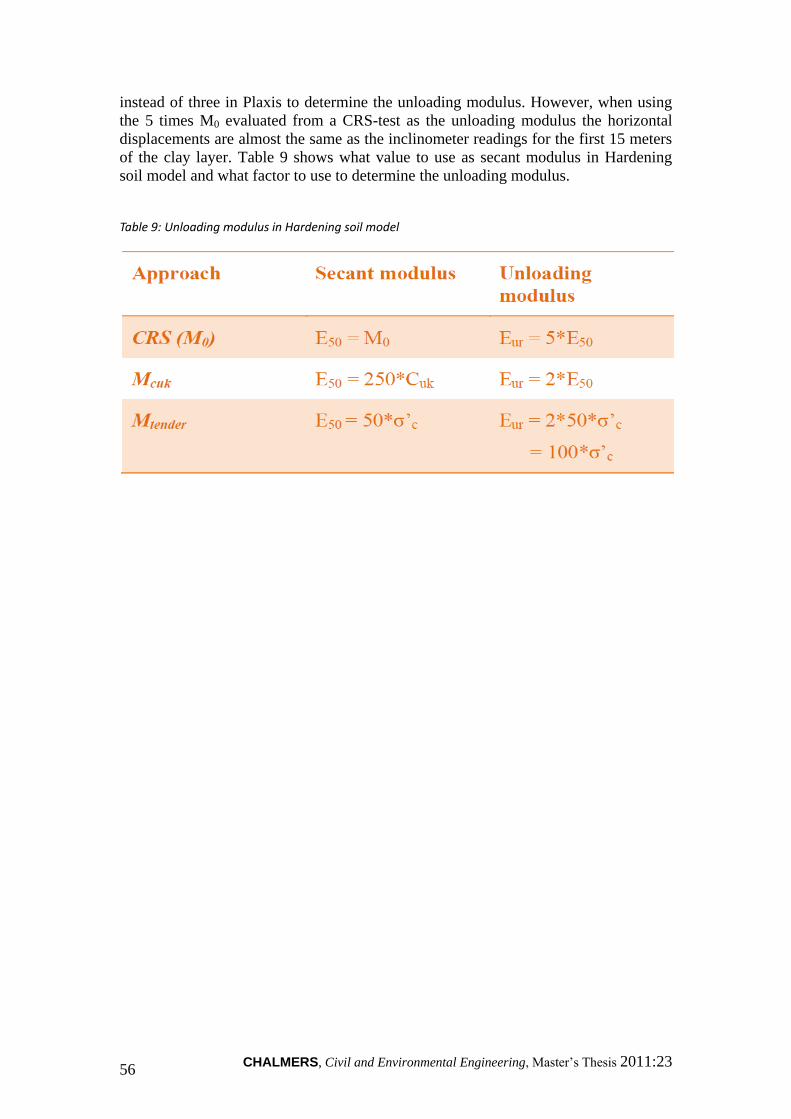
CHALMERS, Civil and Environmental Engineering, Master’s Thesis 2011:23 56
instead of three in Plaxis to determine the unloading modulus. However, when using
the 5 times M0 evaluated from a CRS-test as the unloading modulus the horizontal
displacements are almost the same as the inclinometer readings for the first 15 meters
of the clay layer. Table 9 shows what value to use as secant modulus in Hardening
soil model and what factor to use to determine the unloading modulus.
Table 9: Unloading modulus in Hardening soil model
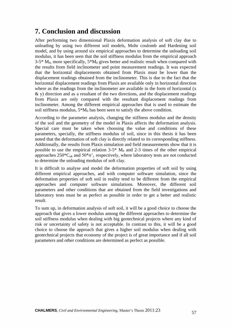
CHALMERS, Civil and Environmental Engineering, Master’s Thesis 2011:23 57
7. Conclusion and discussion
After performing two dimensional Plaxis deformation analysis of soft clay due to
unloading by using two different soil models, Mohr coulomb and Hardening soil
model, and by using around six empirical approaches to determine the unloading soil
modulus, it has been seen that the soil stiffness modulus from the empirical approach
3-5* M0, more specifically, 5*M0 gives better and realistic result when compared with
the results from field inclinometer and point measurement readings. It was expected
that the horizontal displacements obtained from Plaxis must be lower than the
displacement readings obtained from the inclinometer. This is due to the fact that the
horizontal displacement readings from Plaxis are available only in horizontal direction
where as the readings from the inclinometer are available in the form of horizontal (x
& y) direction and as a resultant of the two directions, and the displacement readings
from Plaxis are only compared with the resultant displacement readings from
inclinometer. Among the different empirical approaches that is used to estimate the
soil stiffness modulus, 5*M0 has been seen to satisfy the above condition.
According to the parameter analysis, changing the stiffness modulus and the density
of the soil and the geometry of the model in Plaxis affects the deformation analysis.
Special care must be taken when choosing the value and conditions of these
parameters, specially, the stiffness modulus of soil, since in this thesis it has been
noted that the deformation of soft clay is directly related to its corresponding stiffness.
Additionally, the results from Plaxis simulation and field measurements show that it is
possible to use the empirical relation 3-5* M0 and 2-3 times of the other empirical
approaches 250*Cuk and 50*σ’c respectively, where laboratory tests are not conducted
to determine the unloading modulus of soft clay.
It is difficult to analyse and model the deformation properties of soft soil by using
different empirical approaches, and with computer software simulation, since the
deformation properties of soft soil in reality tend to be different from the empirical
approaches and computer software simulations. Moreover, the different soil
parameters and other conditions that are obtained from the field investigations and
laboratory tests must be as perfect as possible in order to get a better and realistic
result.
To sum up, in deformation analysis of soft soil, it will be a good choice to choose the
approach that gives a lower modulus among the different approaches to determine the
soil stiffness modulus when dealing with big geotechnical projects where any kind of
risk or uncertainty of safety is not acceptable. In contrast to this, it will be a good
choice to choose the approach that gives a higher soil modulus when dealing with
geotechnical projects that economy of the project is of great importance and if all soil
parameters and other conditions are determined as perfect as possible.
CHALMERS, Civil and Environmental Engineering, Master’s Thesis 2011:23 58
8. Recommendations
In this master’s thesis, the deformation analysis soft clay due to excavation in
performed through the help of Plaxis simulation. As stated earlier, it is a bit complex
to catch and model the real behaviour of soft soil due to unloading in Plaxis
simulation. Therefore, increasing the accuracy of the investigation of important soil
parameters and other conditions will not only make the Plaxis simulation less
complicated, but also affects the results from the simulation towards favourable
direction.
The first suggestion is concerned with the soil stiffness modulus which is the aim of
this thesis. Normally, the unloading modulus of soft clay is determined by performing
unloading and reloading test in the oedometer laboratory test. However, this test is not
performed in this thesis. By performing this test a good value of the unloading
modulus can be attained, and this value can be compared with the empirical
approaches and a further better value can be attained. Additionally, better and realistic
results that resemble the deformation behaviour in reality from Plaxis deformation
simulation can be expected.
The other soil parameter that needs further investigation is shear strength. The
undrained shear strength of the clay determined from the field and laboratory tests has
failed to satisfy Hansbo’s relation being lower than the limit value leading to make a
conclusion that further investigation shall be carry out in order to get a reasonable
value.
Last but not least, further investigations on parameters and other conditions that affect
the deformation analysis of soft clay like liquid limit, density and swelling parameters
of the clay, field deformation measurements and influence of structural elements on
the deformation near excavation area shall be carried out in order to increase the
accuracy of the deformation analysis and decrease the probability of occurrence of
errors.
CHALMERS, Civil and Environmental Engineering, Master’s Thesis 2011:23 59
References
Briaud, J.L. (2010): Introduction to soil moduli. Department of Civil Engineering,
A&M University, College Station, Texas, USA, 2010. Available at
http://www.intelligentcompaction.com/downloads/IC_RelatedDocs/SoilCmpct_BR
IAUD_Introduction%20to%20Soil%20Moduli.pdf [Accessed 2011-02-15]
Brinkgreve, R.B.J. et al (2010): Plaxis manuals, 2D-version 10. Delft University of
Technology, The Netherlands.
Brouwer, JJ.M. (2007): In-situ soil testing. Delft University of Technology, {The
Netherlands}, {2007}, 144 pp. Available at : http://www.conepenetration.com
[Accessed 2011-02-13]
Eniro.se. (2011). Available at : www.Eniro.se [Accessed 2011-05-02]
GEOTip (2011): Consistency index, Publisher, {Germany}. Available at:
http://geotip.igt.ethz.ch [Accessed 2011-05-02]
Houlsby, G.T. (1982): Theoretical analysis of the fall cone test. Available at
http://www-civil.eng.ox.ac.uk/people/gth/j/j3.pdf[Accessed 2011-02-27]
Kullingsjö, A. (2007): Effects of deep excavations in soft clay on the immediate
surroundings. Ph.D. Thesis. Department of Civil and environmental Engineering,
Chalmers University of Technology, Göteborg, Sweden, 2007, 334 pp.
Larsson, R. (2008): Jords egenskaper. Statens geotekniska institute (Swedish
geotechnical institute), Infrormation 1, Linköping, {Sweden}, {2008}, 58 pp.
Persson, J. (2004): The unloading modulus of soft clay: A field and laboratory study.
Licentiate thesis. Department of Geo Engineering, Chalmers University of
Technology, Göteborg, Sweden, 2004, 127 pp.
SGI (2007): Deponiers stabilitet, Information 19, Linköping, {Sweden}, {2007}, 46
pp.
SGI (1995): Geotechnical Properties of Clay at Elevated Temperature, Report 47,
Linköping, {Sweden}, {1995}, 69 pp.
CHALMERS, Civil and Environmental Engineering, Master’s Thesis 2011:23 60
Sällfors, G. (2001): Jordmateriallära-Jordemekanik. 3:rd edition. Chalmers
University of Technology, Göteborg, {Sweden}, {2001}, 141 pp.
The comet group program (2011), University Corporation for Atmospheric Research,
Colorado, {USA}, {2011}, Available at: www.meted.ucar.edu [Accessed 2011-02-
13]
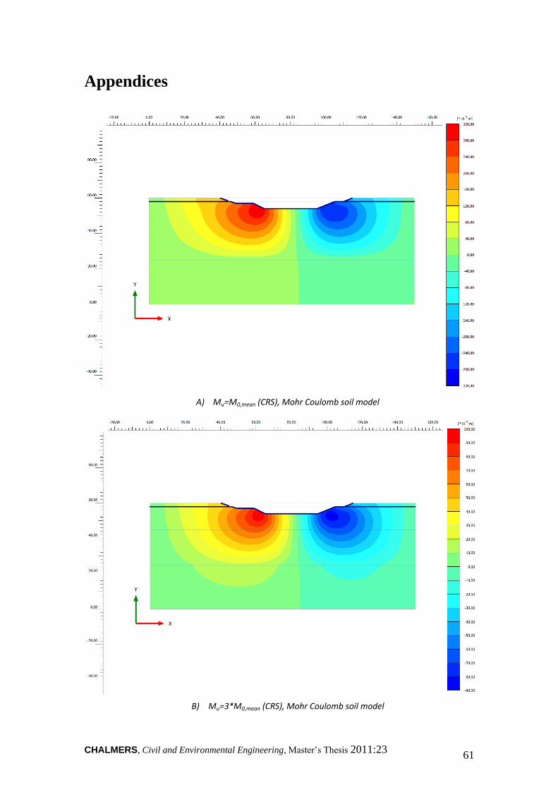
CHALMERS, Civil and Environmental Engineering, Master’s Thesis 2011:23 61
Appendices
A) Mu=M0,mean (CRS), Mohr Coulomb soil model
B) Mu=3*M0,mean (CRS), Mohr Coulomb soil model
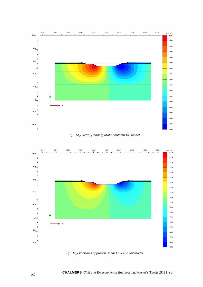
CHALMERS, Civil and Environmental Engineering, Master’s Thesis 2011:23 62
C) Mu=50*σ`c (Tender), Mohr Coulomb soil model
D) Mu= Persson`s approach, Mohr Coulomb soil model

CHALMERS, Civil and Environmental Engineering, Master’s Thesis 2011:23 63
E) Mu=5*M0,mean (CRS), Mohr Coulomb soil model
F) Mu=5*M0,mean (CRS), Hardening soil model

CHALMERS, Civil and Environmental Engineering, Master’s Thesis 2011:23 64
G) Mu=3*250*Cuk, Hardening soil model