large-deformation displacement transfer functions for

NASA/TP—2013–216550

Large-Deformation Displacement Transfer Functions for Shape Predictions of Highly Flexible Slender Aerospace StructuresWilliam L. Ko and Van Tran FleischerDryden Flight Research Center, Edwards, California

Click here: Press F1 key (Windows) or Help key (Mac) for help

December 2013

NASA STI Program ... in Profile

Since its founding, NASA has been dedicated to the advancement of aeronautics and space science. The NASA scientific and technical information (STI) program plays a key part in helping NASA maintain this important role.

The NASA STI program operates under the auspices of the Agency Chief Information Officer. It collects, organizes, provides for archiving, and disseminates NASA’s STI. The NASA STI program provides access to the NASA Aeronautics and Space Database and its public interface, the NASA Technical Reports Server, thus providing one of the largest collections of aeronautical and space science STI in the world. Results are published in both non-NASA channels and by NASA in the NASA STI Report Series, which includes the following report types:

� TECHNICAL PUBLICATION. Reports of completed research or a major significant phase of research that present the results of NASA Programs and include extensive data or theoretical analysis. Includes compila-tions of significant scientific and technical data and information deemed to be of continuing reference value. NASA counter-part of peer-reviewed formal professional papers but has less stringent limitations on manuscript length and extent of graphic presentations.

� TECHNICAL MEMORANDUM. Scientific and technical findings that are preliminary or of specialized interest, e.g., quick release reports, working papers, and bibliographies that contain minimal annotation. Does not contain extensive analysis.

� CONTRACTOR REPORT. Scientific and technical findings by NASA-sponsored contractors and grantees.

� CONFERENCE PUBLICATION. Collected papers from scientific and technical conferences, symposia, seminars, or other meetings sponsored or co-sponsored by NASA.

� SPECIAL PUBLICATION. Scientific, technical, or historical information from NASA programs, projects, and missions, often concerned with subjects having substantial public interest.

� TECHNICAL TRANSLATION. English-language translations of foreign scientific and technical material pertinent to NASA’s mission.

Specialized services also include organizing and publishing research results, distributing specialized research announcements and feeds, providing information desk and personal search support, and enabling data exchange services.

For more information about the NASA STI program, see the following:

� Access the NASA STI program home page at http://www.sti.nasa.gov

� E-mail your question to [email protected]

� Fax your question to the NASA STI InformationDesk at 443-757-5803

� Phone the NASA STI Information Desk at 443-757-5802

� Write to:STI Information DeskNASA Center for AeroSpace Information7115 Standard DriveHanover, MD 21076-1320

This page is required and contains approved text that cannot be changed.

NASA/TP—2013–216550

Large-Deformation Displacement Transfer Functions for Shape Predictions of Highly Flexible Slender Aerospace StructuresWilliam L. Ko and Van Tran FleischerDryden Flight Research Center, Edwards, California

Insert conference information, if applicable; otherwise delete


Enter acknowledgments here, if applicable.

National Aeronautics andSpace Administration

Dryden Flight Research CenterEdwards, CA 93523-0273

December 2013

PATENT PROTECTION NOTICE

The method for structural deformed shape predictions using rectilinearly distributed surface strains and embodied Ko Displacement Transfer Functions for conversions into out-of-plane deflections described in this NASA technical publication is protected under Method for Real-Time Structure Shape-Sensing(Invented by William L. Ko and William Lance Richards), U.S. Patent No. 7,520,176 issued April 21, 2009. Therefore, those interested in using the method should contact The NASA Innovative Partnership Program Office, NASA Dryden Flight Research Center, Edwards, California for more information.


Available from:


NASA Center for AeroSpace Information7115 Standard Drive

Hanover, MD 21076-1320443-757-5802

v

TABLE OF CONTENTS

ABSTRACT............................................................................................................................................... 1

NOMENCLATURE .................................................................................................................................. 1

INTRODUCTION ..................................................................................................................................... 2

CURVATURE-STRAIN RELATIONSHIP.............................................................................................. 4

DIFFERENT CURVATURE EQUATIONS............................................................................................. 4Classical (Eulerian) Curvature Equation............................................................................................... 4Physical (Lagrangian) Curvature Equation........................................................................................... 5Shifted Curvature Equation................................................................................................................... 6

CURVATURE-STRAIN DIFFERENTIAL EQUATIONS ...................................................................... 7

NONUNIFORM AND UNIFORM BEAMS............................................................................................. 8

SHIFTED DISPLACEMENT TRANSFER FUNCTIONS....................................................................... 8Based on Piecewise Linear Strain Representations............................................................................... 8

Nonuniform Beams............................................................................................................................ 9Slightly Nonuniform Beams .............................................................................................................. 9First Order Expansion.......................................................................................................................10Second Order Expansion ..................................................................................................................11

Based on Piecewise Nonlinear Strain Representations........................................................................11Improved Case ..................................................................................................................................12Log-expanded Case ..........................................................................................................................13Depth-expanded Case .......................................................................................................................13

Characteristics of Displacement Transfer Functions ...........................................................................14

EULERIAN FORMULATION OF DISPLACEMENT TRANSFER FUNCTIONS ..............................15Projected Domain Lengths...................................................................................................................15Slope Equation .....................................................................................................................................16Deflection Equation .............................................................................................................................17Log-Expanded Slope Equation ............................................................................................................18Log-Expanded Deflection Equation.....................................................................................................19Simplified Deflection Equation ...........................................................................................................19

LAGRANGIAN FORMULATION OF DISPLACEMENT TRANSFER FUNCTIONS........................20Slope Equation .....................................................................................................................................21Deflection Equation .............................................................................................................................22Simplified Deflection Equation ...........................................................................................................23

STRUCTURE USED FOR SHAPE PREDICTION ACCURACY STUDIES ........................................23Finite-Element Analysis.......................................................................................................................23Surface Strains .....................................................................................................................................24

COMPARISONS OF SHAPE PREDICTION ACCURACIES ...............................................................24Slope Predictions..................................................................................................................................24

vi

Slope Curves ........................................................................................................................................27Deflection Predictions..........................................................................................................................27Deflection Curves ................................................................................................................................30

SHAPE PREDICTION ERROR CURVES ..............................................................................................30Slope-Error Curves ..............................................................................................................................30Deflection-Error Curves.......................................................................................................................31

EXPERIMENTAL VALIDATIONS OF SHAPE-PREDICTION ACCURACIES.................................32

DISCUSSIONS.........................................................................................................................................33

CONCLUDING REMARKS....................................................................................................................34

FIGURES..................................................................................................................................................36

APPENDIX A: ALTERNATIVE DERIVATION OF THE PHYSICAL (LAGRANGIAN)CURVATURE EQUATION................................................................................................................47

APPENDIX B: GRAPHICAL DERIVATION OF THE SHIFTED CURVATURE EQUATION .........50

APPENDIX C: DERIVATION OF PROJECTED DOMAIN LENGTH FOR EULERIAN FORMULATION............................................................................................................52

APPENDIX D: DERIVATIONS OF THE EULERIAN SLOPE EQUATIONS .....................................53

APPENDIX E: DERIVATIONS OF LAGRANGIAN SLOPE EQUATION ..........................................57

REFERENCES .........................................................................................................................................58

1

ABSTRACT

Displacement Transfer Functions were formulated for deformed shape predictions of structures under large deformations. By discretization of the embedded beam (depth-wise cross section of structure along the surface strain-sensing line), the distributions of surface bending strains could be represented with piecewise linear functions. Such a piecewise approach enabled piecewise integrations of the curvature equations (Eulerian, Lagrangian, and Shifted curvature equations) of the deformed embedded-beam to yield closed-form Displacement Transfer Functions, which are expressed in terms of embedded beam geometrical parameters and surface strains. By inputting the surface strain data, the Displacement Transfer Functions can then transform the surface strains into deflections for mapping out the overall structural deformed shapes for visual display. A long tapered cantilever tubular beam was chosen for studying the large-deformation shape predictions. The input surface strains were analytically generated from finite-element analysis. Also, the finite-element generated slopes and deflections were used as reference yardsticks to study the theoretical shape prediction accuracies. The Displacement Transfer Functions based on the Shifted curvature equation were found to be amazingly accurate beyond expectation. However, the Displacement Transfer Functions based on the Eulerian and Lagrangian curvature equations, resulted in very complex mathematical expressions, and gave very poor shape predictions at large deformations.

NOMENCLATUREc depth factor (vertical distance from neutral axis to bottom surface of uniform beam), inc(s) depth factor (vertical distance from deformed neutral axis to bottom surface of nonuniform

embedded beam), inc(x) depth factor (vertical distance from undeformed neutral axis to bottom surface of nonuniform

embedded beam), inic depth factor (vertical distance from neutral axis to i-th strain-sensing station on bottom

surface of nonuniform embedded beam), in0c value of ic at fixed end (beam root), 00 �� xx , in

nc value of ic at free end (beam Math equationsp), lxx n �� , inDLL design limit loadE Young’s modulus, lb/in2

i n,....,3,2,1,0� , strain-sensor identification number, or an imaginary unit, 1��il length of embedded beam, inn index for the last span-wise strain-sensing station (or number of domains) R radius of curvature, inR�

averaged radius of curvature for domain, ii xxx ��1 , in RRF Rotated reference frameSPAR Structural Performance And Resizing finite element computer program STS Space Transport System for the Space Shuttle flightss curved coordinate along deformed embedded beam elastic curve, inu axial displacement, inx, y Cartesian coordinates (x in beam axial direction, y in lateral direction), in

axial coordinate of -th strain sensor (or strain-sensing station at ), in )(xy beam deflection at axial location x, in

y� curved deflection (curved distance traced by the same material point from its initial un-deformed position to its final deformed position, in

iy )( ixy� , beam deflection at axial location, ixx � , in

2

V )(tan/ xdxdy �� , beam slope, in/in

iV )( ixV� , value of V at strain-sensing station, in/innlxx ii /)( 1 �� , domain length (distance between two adjacent strain-sensing stations 1{ �ix , }ix ,

incl� chord length of arc formed by bent , in

iL� projected domain length on the x-axis of bent and tilted , in �(s) surface bending strain at curved locationn , in/in�(x) surface bending strain at axial locationn , in/in

i , surface bending strain at strain-sensing station, , in/in

s axial strain in s-direction, in/in)(s� beam slope in reference to s-system, rad or deg)(x� beam slope in reference to x-system, rad or deg

i� )( ix�� , slope at strain-sensing station, ixx � , rad or deg

n� )( nx�� , slope at beam tip strain-sensing station, lxx n �� , rad or deg 1�� ixx , local axial coordinate for domain, ii xxx ��1 , in

INTRODUCTIONFor structure (for example, aircraft wings) deformed shape predictions using discretely distributed

surface strains (bending strains), the Displacement Transfer Functions (refs. 1–5) are needed to convert the surface strains into out-of-plane deflections so that one can plot the overall structural deformed shape for visual display. The surface strains are to be obtained from the strain-sensing stations evenly distributed along each strain-sensing line on the surfaces of the structure. The depth-wise cross section of the structure along the surface strain-sensing line can then be considered as an imaginary embedded beam. In the formulations of earlier Displacement Transfer Functions (refs. 1–5), the embedded beam was first evenly divided into multiple small domains, with domain junctures matching the strain-sensing stations. Thus, within each small domain, the beam depth factor could be described with a linear function, and the surfacestrain variation could be described with either linear or nonlinear function. Such piecewise approach enabled the piecewise integrations of the curvature equation [classical (Eulerian), physical (Lagrangian), and Shifted curvature equations] for the elastic curve of each deformed embedded beam to yield closed-form slope and deflection equations in recursive forms. Those recursive slope and deflection equations were then combined into a single deflection equation in dual summation form (called the Displacement Transfer Function), which is expressed in terms of embedded beam geometrical parameters and discretely distributed surface strains. By inputting the surface strain data into the Displacement Transfer Function, one can then calculate deflections along each embedded beam. By using multiple strain-sensing lines, the overall structural deformed shape (induced by bending and torsion) can be geometrically mapped out for visual display.

The Displacement Transfer Functions (in different mathematical forms for different types of structural geometry) developed by Ko (refs.1–5), can be used to calculate deflections from strain data obtained from the fiber optic strain-sensing method introduced by Richards (ref. 6) to create a revolutionary structure-shape-sensing technology called; “Method for Real-Time Structure Shape-Sensing,” U.S. Patent Number 7,520,176 (Ko-Richards), (ref. 6). This patented technology is quite attractive to the in-flight deformed shape monitoring of highly flexible wings of unmanned flight vehicles by the ground-based pilot for maintaining safe flights. In addition, the real time wing shape monitored could then be input to the aircraft control system for aero-elastic wing shape control.

The surface strain data for inputs to the Displacement Transfer Functions (ref. 1–5) for shape predictions can be obtained from the conventional strain gages, from fiber optic strain sensors, or

3

analytically calculated from finite-element analysis. It is important to mention that without the use of the Displacement Transfer Functions, any type of surface strain sensors can only sense the strains, but not the out-of-plane deflections nor the cross-sectional rotations of the structure.

The distributed fiber optic surface strains can also be input to the Displacement Transfer Functions, the Stiffness and Load Transfer Functions to calculate structural stiffness (bending and torsion), and operationalloads (bending moments, shear loads, and torques) for monitoring the flight-vehicle’s operational loads. This patented method is called “Process for Using Surface Strain Measurements to Obtain Operational Loads for Complex Structures,” U.S. Patent No. 7,715,994 (Richards-Ko), (ref. 7). The accuracy of thispatented method for estimating operational loads on structures was analytically confirmed by using finite-element analysis of different aerospace structures (tapered cantilever tubular beam, depth-tapered un-swept wing box, depth-tapered swept wing box, and doubly-tapered generic long-span wing) (ref. 8).

The earlier Displacement Transfer Function (refs. 1–5) were analytically validated for prediction accuracies by finite-element analysis of different sample structures such as cantilever tubular beams (uniform, tapered, slightly tapered, and step-wisely tapered), two-point supported tapered tubular beams, flatpanels, and tapered wing boxes (un-swept and swept).

To eliminate mathematical indeterminacy at the limit of uniform beam depth, additional First-Order and Second-Order displacement transfer functions (ref. 9) were formulated for structural deformed shape predictions. The prediction accuracies of the two new Displacement Transfer Functions were found to be comparable with those of the earlier Displacement Transfer Functions (refs. 1–5).

Also, by using piecewise nonlinear (instead of piecewise linear) strain representations in theformulations of the improved Displacement Transfer Functions (ref. 10), the shape prediction accuracies could be improved greatly especially for highly tapered slender structures.

The earlier Displacement Transfer Functions (refs. 1–5) were formulated for the straight beams. However, by introducing empirical curvature-effect correction terms, the resulting modified Displacement Transfer Functions could be applied to the shape predictions of slender curved structures (including full-circle structures), with great success (ref. 11).

All the past Displacement Transfer Functions were formulated by integrating the beam curvature equation in reference to the undeformed fixed coordinate system, and were found to be amazingly accurate for the shape predictions of various slender structures under small bending deformations.

For certain new type of unmanned aircraft such as Global Observer, with highly flexible wing structures having long wingspan reaching 175 ft, the wing tip deflection could reach up to 32 ft during flights. For the shape predictions of such type of highly flexible structures, there is a need to formulate large-deformation Displacement Transfer Functions.

The present technical publication discusses different curvature equations [classical (Eulerian), physical (Lagrangian), and Shifted curvature equations] for the embedded beam elastic curves, referred to deformed or undeformed coordinate systems. This technical publication describes the formulations of different large-deformations Displacement Transfer Functions through beam discretization and piecewise integrations of the said different curvature equations.

A long tapered cantilever tubular beam was used in the shape prediction accuracy analysis of the newly formulated Displacement Transfer Functions. The input surface strains in the present technical publicationwere analytically generated from the finite-element analysis of the tapered cantilever tubular beam. For the

4

shape prediction accuracy studies of the newly formulated Displacement Transfer Functions, the slopes and deflections calculated from the finite-element analysis were used as reference yardsticks.

CURVATURE-STRAIN RELATIONSHIPFigure 1 shows the deformed state of a nonuniform beam with changing depth factor, c(s). The

curvature-strain relationship can be established graphically from figure 1. The beam elastic curve has local radius of curvature, R(s), within a small beam segment subtended by �d . The un-deformed curve length, AB, lies on the beam neutral surface, and the deformed curve length, ��(s)]} [where �(s) is the surface strain], lies on the beam bottom surface. From the two similar slender sectors, ABO� and BAO �� ,the following relationship can be established:

(1)

From equation (1) the following curvature-strain equation is obtained:

(2)

Equation (2) geometrically relates the local curvature, 1/R(s), of the deformed beam elastic curve to the associated surface strain, �(s), and the beam depth factor, c(s). Equation (2) was the basis for the formulations of the earlier Displacement Transfer Functions (ref. 1–5), and is also used in the present technical publication to formulate the Displacement Transfer Functions for large deformations.

DIFFERENT CURVATURE EQUATIONSThis section discusses three types of curvature equations for deformed beam elastic curve: 1) classical

(Eulerian) curvature equation, 2) physical (Lagrangian) curvature equation, and 3) Shifted curvature equation. These three curvature equations will be geometrically related to surface strains and beam depth factor for establishing three curvature-strain differential equations for the formulations of the large-deformation displacement transfer functions.

Classical (Eulerian) Curvature Equation

The derivation of the classical curvature equation for a plane curve can be found in any standard calculus textbook, and are presented in the following paragraphs for the purpose of refreshing memory.

From figure 1, the infinitesimal curved segment, , and the local slope,

)/(tan 1 dxdy�� , can be used to express the curvature, dsdR //1 �� , in the following forms (see slender sector, ABO� in figure 1) (ref. 12):

(3)

5

Equation (3) is the classical mathematical curvature equation for a plane curve, and can be found in any standard calculus textbook.

When equation (3) is applied to describe the curvature of the deformed-beam elastic curve, the x-variable in equation (3) will now denote the abscissa of any material point on the elastic curve in its final deformed position (Eulerian description), (fig. 1). Thus, based on equation (3), a certain x-coordinate of a material point in the deformed configuration no longer represents the same material point in the undeformed state. Namely, the deformed material point has no memory of its initial undeformed x-location. As will be seen shortly, the slope equation formulated based on equation (3) gave erroneous slope data, and causeddeflection predictions to be poor at large deformations. For more detailed discussions of the classical curvature equation (3), please see references 13�16.

It must be mentioned that the classical Euler-Bernoulli beam theory was formulated based on the linearized classical (Eulerian) curvature equation (3) [that is, the term 2)/( dxdy neglected], which was referred to the deformed x-coordinate. For small deflections, the difference between the deformed and undeformed x-coordinates is negligible; however, for large bending deformations the two x-systems can be quite different.

Physical (Lagrangian) Curvature Equation

As shown in figure 2, the infinitesimal curved segment, ds, of the deformed-beam elastic curve in the limit could be considered as an infinitesimal straight-line segment. Then, the local slope, )(s� , along the s-curve can be expressed as )/(sin)( 1 dsdys �� . The local curvature expressed in reference to the s-system, can then be written as equation (4):

(4)

In general, under bending deformation, the original undeformed length, dx, along the beam x-axis will be deformed into arc length, ds, along the s-curve (fig. 2). Then, one can write:

(5)

in which is the axial strain in s-direction. For an in-extensional beam, �(s)=0, and equation (5) becomes:

(6)

Equation (6) shows that for the in-extensional beam, the s-coordinate of any material point in the deformed configuration is always equal to its initial undeformed x-coordinate. In view of equation (6), the curvature equation (4) can be rewritten in reference to the undeformed x-coordinate as:

(7)

6

Equation (7) is the physical (Lagrangian) curvature equation for the elastic curve of an in-extensional beam expressed in reference to the undeformed x-coordinate (Lagrangian description). Equation (7) was also derived by Kopmaz (ref. 13) and Hodge (ref. 14) based on kinematics of a deformed beam (fig. 2). The alternative derivation of equation (7) is described in Appendix A.

It is important to mention that for an in-extensional beam ( dxds � ), (fig. 2), when the s-system is converted into the undeformed x-system, )/)((sin dsdys �� in the s-system will become )/)((tan dxdyx ��in the x-system [that is, )(tan)(sin xs �� ]. Thus, the slope, )(x� , in the x-system will be slightly smaller than the slope, )(s� in the s-system. Therefore, the line EA� drawn from point A� (fig 2) to define the slope, )(x� , in the x-system will be slightly tilted away from the true tangent to the s-curve at point A�(fig. 2). However, this slope-tilt is miniscule because the axial displacements induced by the lateral bending are quite small.

Shifted Curvature Equation

The formulations of the Shifted Displacement Transfer Functions are based on the undeformed x-coordinate. Namely, the deformed material points are shifted back in the x-direction and plotted at their respective initial undeformed x-coordinates (fig. 3). Thus, the Shifted curvature equation to be formulated will be slightly different from the physical curvature equation (7) for which the deformed configuration of the beam is described with the un-deformed fixed coordinate system (that is, no horizontal shifting of deformed material points).

From a small right triangle CBA �� (fig. 2), the following relationship holds:

222 )( dydudxds �� (8)

in which u (= AA �� ), (fig 2) is the x-displacement (axial direction) of a material point A. In view of equation (8), the physical curvature, equation (4), in the s-system can be rewritten as:

(9)

Because in the beam bending deformations, the axial displacement, u, of a material point is quite small, it is reasonable to set 0 u , which is equivalent to horizontal shifting of the deformed material points like

A�{ , }B� (fig. 3) toward the right to the positions A ��{ , }B �� with x-coordinates respectively matching the initial x-coordinates of the un-deformed positions A{ , }B .

Under the condition, 0 u , equation (9) becomes:

(10)

7

For an in-extensional beam, the curved coordinate, s, of any deformed material point is always equal to its initial undeformed coordinate x (fig. 3); namely, xs � and dxds � [ eq. (6)]. Then equation (10) can be written in the un-deformed x-system as:

(11)

Equation (11) is called the Shifted curvature equation for the in-extensional beam ( dxds � ), referred to the undeformed x-coordinate. Equation (11) can also be established graphically in view of figure 3 (see Appendix B).

The mathematical form of equation (11) is equivalent to the linearized form of the Lagrangian curvature equation (7) [the term 2)/( dxdy dropped] because both equations (7) and (11) are referred to the undeformed x-coordinate (figs. 2, 3). It is important to mention that, for an in-extensional beam, setting

0 u (that is, shifting deformed material points and plot at their respective undeformed x-locations) causes 2)/( dxdy �0 according to equation (A8) in Appendix A and, therefore, implying linearization of the

Lagrangian curvature equation (7).

However, equation (11) cannot be equivalent to the linearized Eulerian curvature equation (3) [the term2)/( dxdy removed] even with similar mathematical forms because, equation (11) is referred to the

undeformed x-coordinate, while equation (3) is referred to the deformed x-coordinate (fig. 1). For small bending deformations, the difference between the deformed and un-deformed x-coordinates could be negligible; however, for large bending deformations, the two x-systems could be quite different.

As will be seen shortly, the Displacement Transfer Functions formulated based on the Shifted curvature equation (11) turned out to be amazingly accurate beyond expectation for large-deformation shape predictions (for example, cantilever beam-tip slope reaching even as large as 66° under bending).

The unexpected discovery in the present technical publication is that the linearized curvature equation used in the formulations of earlier Displacement Transfer Functions (refs. 1–5) was not referred to the deformed x-coordinate, but to the undeformed x-coordinate. Therefore, the earlier linearized curvature equation was actually the Shifted curvature equation (11), and the Displacement Transfer Functions formulated based on equation (11) were found to be amazingly accurate beyond expectation in the structural deformed shape predictions.

CURVATURE-STRAIN DIFFERENTIAL EQUATIONSIn view of equation (2), the Eulerian, Lagrangian, and the Shifted curvature equations (3), (7), and (11)

can be written respectively in the forms of curvature-strain differential equations for the deformed beam as:

1. Eulerain curvature-strain differential equation:

(12)

8

2. Lagrangian curvature-strain differential equation:

(13)

3. Shifted curvature-strain differential equation:

(14)

The formulations of the large-deformation displacement transfer functions stemmed from the integrations of the curvature-strain differential equations (12)–(14). Note that, equations (12)–(14) are purely geometrical relationships, containing no material properties. Likewise, the Displacement Transfer Functions formulated by integrating equations (12)–(14) will also contain no material properties. In fact, the material properties will affect the outputs of the surface strains, )(x (refs. 1–5).

NONUNIFORM AND UNIFORM BEAMSIn the present technical publication, the term “beam” implies the imaginary embedded beam (the

depth-wise cross section of the structure along the surface strain-sensing line), and not the classical isolated Euler-Bernoulli beams. The nonuniform beam in the present technical publication is defined as the embedded beam with a varying depth factor, )(xc , a vertical distance from the neutral axis to the bottom surface of the nonuniform beam at axial location, . For a nonuniform tubular beam, )(xc will be the outward radius. The uniform beam in the present technical publication is defined as the embedded beam with constant depth factor [that is, cxc �)( ].

SHIFTED DISPLACEMENT TRANSFER FUNCTIONSIn the formulations of earlier Displacement Transfer Functions (refs. 1–5) for structural deformed shape

predictions, the curvature-strain differential equation used turned out to be equivalent to the Shifted-curvature-strain differential equation (14). Therefore, there is no need to reformulate the large-deformation Displacement Transfer Functions based on the Shifted curvature-strain differential equation (14). The Displacement Transfer Functions formulated earlier can be called Shifted Displacement Transfer Functions, which, as will be shown shortly, were found to be amazingly accurate beyond expectations for the shape predictions not only for small deformations, but also for very large deformations.

The Shifted Displacement Transfer Functions formulated earlier for equal domain length ( =constant) (refs. 1–5) are reproduced in the following sections. Keep in mind that the slopes, ])/()([ iii dxdyx ��

),....,3,2,1( ni � , at the strain-sensing stations, , appearing in the following Shifted Displacement Transfer Functions are referred to the initial undeformed x-coordinates.

Based on Piecewise Linear Strain Representations

The following four sets of Shifted slope and deflection equations [eqs. (15)–(18)] were formulated by using piecewise-linear functions to describe the distributions of both surface strains and depth factors,

)({ x , )}(xc .

9

1. Nonuniform Beams (refs. 1, 3)

Slope equation:

11

21

11

1

1 tanlog)(

tan ��

��

�

� ��

��

��

��

�� ii

i

ii

iiii

ii

iii c

ccc

cccc

l �� ; ),....,3,2,1( ni � (15a)

Deflection equation:

a. In recursive form:

1111

31

11

1

12 tan)(log)()(2

)( ��

��

�

� ��

��

��

��

��

��

��

�� iiiii

ii

ii

iiii

ii

iii lycc

ccc

cccc

ccly �

),....,3,2,1( ni �

(15b)

b. In dual summation form:

��

��

beamscantileverfor 0=

00

termsslopefromonContributi

1

1 12

1

11

1

12

termsdeflectionfromonsContributi

11

13

1

11

1

12

tan)(log)(

)()(

)(log)()(2

)(

�

liycc

cccc

ccjil

cccc

ccc

cccc

ly

i

j j

je

jj

jjjj

jj

jj

i

jjj

j

jej

jj

jjjj

jj

jji

��

��

��

��

��

�

��

�

�

��

�

��

��

��

��

��

��

�

��

��

�

��

�

��

!

!

�

� ��

��

�

�

��

��

��

�

�

),....,3,2,1( ni �

(15c)

Equation (15c) is called the Nonuniform Displacement Transfer Function.

2. Slightly Nonuniform Beams [ elog terms in equations (15a)–(15c) expanded] (refs. 1, 3)

Slope equation:

1111

tan22

tan ��

��

��

��

�

��

��

�� iii

i

i

ii c

cc

l �� ; ),....,3,2,1( ni � (16a)



11111

2

tan36

)(��

��

��

��

��

�

��

��

�� iiii

i

i

ii ly

cc

cly � ; ),....,3,2,1( ni � (16b)

10


��

��


00

termsslopefromonsContributi

1

11

11

2

termsdeflectionfromonContributi

11

11

2

tan

2)(2)(31

6)(

�

ly

cc

cjil

cc

cly

i

jjj

j

j

j

i

jjj

j

j

ji

��

��

��

��

��

��

�

��

��

��

��

��

��

��

��

��

��

��

�

��

��

��

��

��

�� !!

�

��

��

��

(16c)

),....,3,2,1( ni �

Equation (16c) is called the Slightly-Nonuniform Displacement Transfer Function.

3. First Order Expansion of )(/1 xc (ref. 8)

Slope equation:

11

111

tan2546

tan ��

��

��

��

��

��

��

�

��

��

�� ii

i

ii

i

i

ii c

ccc

cl �� ; (17a)



111

111

2

tan3512

)(��

��

��

��

��

��

��

��

�

��

��

�� iii

i

ii

i

i

ii ly

cc

cc

cly � ; ),....,3,2,1( ni � (17b)


��

��

beamscantiteverfor 0=

00


1

1 11

11

2


1 11

11

22

tan254)(6

)(

35)(12

)(

�

lycc

cc

cjil

cc

cc

clly

i

jj

j

jj

j

j

i

i

jj

j

jj

j

j

ji

��

�

��

��

��

��

��

��

��

��

��

�

��

��

��

��

��

��

��

��

!

!

�

� ��

��

� ��

��

(17c)

),....,3,2,1( ni �

Equation (17c) is called the First-Order Displacement Transfer Function.

11

4. Second Order Expansion of )(/1 xc (ref. 8)

Slope equation:

1

2

111

2

111tan3101349

12tan �

��

��

��

��

��

��

��

�

��

��

��

��

��

�

��

��

��

��

�� ii

i

i

i

ii

i

i

i

i

ii c

ccc

cc

cc

cl �� (18a)

),....,3,2,1( ni �Deflection equation:


11

2

111

2

111

2

tan31118292760

)(��

��

��

��

��

��

��

��

�

��

��

��

��

��

�

��

��

��

��

�� iii

i

i

i

ii

i

i

i

i

ii ly

cc

cc

cc

cc

cly � (18b)

),....,3,2,1( ni �


��

��

��


00


1

1

2

111

2

111

2


1

2

111

2

111

2

tan)(

3101349)(12

)(

311182927160

)(

�

liy

cc

cc

cc

cc

cjil

cc

cc

cc

cc

cly

i

jj

j

j

j

jj

j

j

j

j

j

i

jj

j

j

j

jj

j

j

j

j

ji

��

��

��

��

��

��

�

�

��

�

�

��

��

��

��

�

�

��

�

�

��

��

��

��

��

��

��

��

��

�

�

��

�

�

��

��

��

��

�

�

��

�

�

��

��

��

��

!

!

�

� ��

��

� ��

��

(18c)

),....,3,2,1( ni �

Equation (18c) is called the Second-Order Displacement Transfer Function.

Based on Piecewise Nonlinear Strain Representations

The following three sets of Shifted slope and deflection equations [eqs. (19)–(21)] were formulated by using piecewise-nonlinear function to describe the actual distribution of the surface strain, )(x , but using piecewise-linear function to describe the actual distribution of the depth factor, )(xc .

12

1. Improved Case (ref. 9)Slope equation:

(19a)

),....,3,2,1( ni �

Deflection Equations:


" #

" # 111111121

2

11

1111141

2

tan)2()25(2)58()(12

)(

)(log)2)(2()(2

)(

��

��

��

��

�

��

��

��

��

�

iiiiiiiiiiiii

iii

ieiiiiiiiiii

iii

lycccccccc

l

ccccccccccc

ccly

�

(19b)

),....,3,2,1( ni �


" #

" #��

termsdeflectionfromonContributi

1111112

1

11

11111412

)2()25(2)58()(12

1

)(log)2)(2()(2

1

)( !�

��

��

��

��

�

��

�

�

��

�

��

�

��

�

��

�

��

��

��

i

jjjjjjjjjj

jj

jjj

jejjjjjjjjjj

jji

cccccccc

cccc

ccccccccc

ly

" #

" #

��

��


00


1

1111112

1

1111113

12

tan)(

)()3(2)35()(4

1

log)2)(2()(2

1

)()(

�

liy

cccccccc

cc

cccccccc

jili

jjjjjjjjjj

jj

j

jejjjjjjjjj

jj

��

��

��

�

��

��

��

�

��

�� !�

��

�

��

�

(19c)

),....,3,2,1( ni �

Equation (19c) is called the Improved Displacement Transfer Function.

13

2. Log-expanded Case [ terms in equation (19a, b, c) expanded] (ref. 9)

Slope equation:

(20a)

),....,3,2,1( ni �



" #" # " #

11

12

12

1112

1

13

132

113

14

1

2

tan)(2)83)((3(2

)(3)38)((724

)(

��

��

��

�

��

��

��

��

��

��

��

ii

iiiiiiiiiiii

iiiiiiiii

ii

lycccccccccc

cccccccccly

�

(20b)),....,3,2,1( ni �


(20c)

),....,3,2,1( ni �

Equation (20c) is called the Log-Expanded Displacement Transfer Function.

3. Depth-expanded Case [expansion of )(/1 xc ] (ref. 9)

Slope equation:

tan)312(1

)103(1)85(224

tan

111

2

1

111

111

��

��

��

��

��

�

��

��

��

��

�

��

��

��

iiiii

i

iiii

iiii

ii

cc

cc

cl

�

�

(21a)

),....,3,2,1( ni �

14



$ % $ %

$ % 1111

2

1

111

111

2

tan312151

7415267

24)(

��

��

��

��

��

�

��

��

��

��

�

��

��

��

iiiiii

i

iiii

iiii

ii

lycc

cc

cly

�

(21b)

),....,3,2,1( ni �


$ % $ %

$ %��


111

2

1

111

11

1

2

312151

7415267

124

)( !�

��

��

��

�

��

�

�

��

�

�

��

��

��

��

��

��

��

i

jjjj

j

j

jjjj

jjjj

ji

cc

cc

cly

��

��


00


11

2

1

111

111

1 1

2

tan)(

)312(1

)103(1)85(2)(

24)(

�

liy

cc

cc

cjil

jjjj

j

jjjj

jjjj

i

j j

��

��

�

�

��

�

�

��

��

��

��

��

��

��

��

��

��

� �!

(21c)

),....,3,2,1( ni �

Equation (21c) is called the Depth-Expanded Displacement Transfer Function.

Characteristics of Displacement Transfer Functions

In each of the Displacement Transfer Functions [eqs. (15c)�(21c)], the deflection, , at the strain-sensing station, , is expressed in terms of the inboard beam depth factors, , andthe associated inboard surface strains, , including the values of at the strain-sensing station where deflection, , is calculated. It is important to mention that equations(15c)�(21c) are purely geometrical relationships, containing no material properties. In fact, the values of the surface strains, , can be affected by the material properties and internal structural configurations.

Thus, in using equations (15c)�(21c) for shape predictions of complex structures such as long-span aircraft wings, there is no need to know the material properties, nor the complex geometries of the internal structures. As will be seen shortly, the Shifted Displacement Transfer Functions [eqs. (15c)�(21c)] turned out to be amazingly accurate beyond expectations for the shape predictions of a long cantilever tapered tubular beam under large bending deformations with beam tip slope even reaching as large as �n �� deg.

15

EULERIAN FORMULATION OF DISPLACEMENT TRANSFER FUNCTIONS

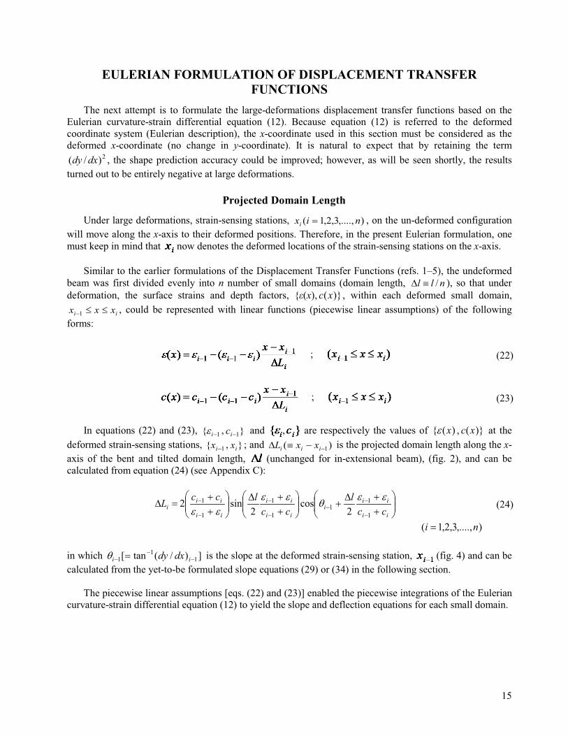
The next attempt is to formulate the large-deformations displacement transfer functions based on the Eulerian curvature-strain differential equation (12). Because equation (12) is referred to the deformed coordinate system (Eulerian description), the x-coordinate used in this section must be considered as the deformed x-coordinate (no change in y-coordinate). It is natural to expect that by retaining the term

2)/( dxdy , the shape prediction accuracy could be improved; however, as will be seen shortly, the results turned out to be entirely negative at large deformations.

Projected Domain Length

Under large deformations, strain-sensing stations, ),....,3,2,1( nixi � , on the un-deformed configuration will move along the x-axis to their deformed positions. Therefore, in the present Eulerian formulation, one must keep in mind that now denotes the deformed locations of the strain-sensing stations on the x-axis.

Similar to the earlier formulations of the Displacement Transfer Functions (refs. 1–5), the undeformed beam was first divided evenly into n number of small domains (domain length, nll /�� ), so that under deformation, the surface strains and depth factors, {�(x), )}(xc , within each deformed small domain,

ii xxx ��1 , could be represented with linear functions (piecewise linear assumptions) of the following forms:

; (22)

; (23)

In equations (22) and (23), 1{ �i , }1�ic and , are respectively the values of )({ x , )}(xc at the deformed strain-sensing stations, 1{ �ix , }ix ; and )( 1�� iii xxL is the projected domain length along the x-axis of the bent and tilted domain length, (unchanged for in-extensional beam), (fig. 2), and can be calculated from equation (24) (see Appendix C):

��

��

��

��

��

��

��

��

��

��

��

�

�

�

�

ii

iii

ii

ii

ii

iii cc

lcc

lccL1

11

1

1

1

1

2cos

2sin2 �

(24)

),....,3,2,1( ni �

in which ])/(tan[ 11

1 ��

� � ii dxdy� is the slope at the deformed strain-sensing station, (fig. 4) and can be calculated from the yet-to-be formulated slope equations (29) or (34) in the following section.

The piecewise linear assumptions [eqs. (22) and (23)] enabled the piecewise integrations of the Eulerian curvature-strain differential equation (12) to yield the slope and deflection equations for each small domain.

16

Slope Equation

Let )(tan/ xdxdyV �� , then the Eulerian curvature-strain differential equation (12) can be written as:

(25)

In view of piecewise linear assumptions [eqs. (22) and (23)], the piecewise-integration of equation (25) within each deformed small deformed domain, , can be written as:

; (26)

in which the lower limit of integral, 1�iV , is the value of V at the deformed strain-sensing station, ,namely, 1111 tan)(tan)( �� iiii xxVV �� .

Integration of equation (26) to obtain the slope equation in closed form is relatively easy; however, subsequent integration of the slope equation to obtain the deflection equation in neat closed-form turned out to be a nightmare, and an alternative simplified approach had to be introduced as discussed in the subsequent sections.

After carrying out integration of equation (26), one obtains equation (27) (ref. 17, and Appendix D):

��

��

��

��

��

��

��

��

��

��

��

�

��

��

�

�

�

� 11log)(

)(11

1

12

1

111

1

121

12

i

i

i

ie

ii

iiiiii

ii

ii

i

i

Lxx

cc

ccccLxx

ccV

V

V

V

)( 1 ii xxx ��

(27)

By squaring both sides, rearranging, then taking the square root, and writing )(tan)( xxV �� , one obtains the slope equation in the following form (see Appendix D):

2

1

12

1

111

1

1

12

1

1

12

1

111

1

1

12

1

11log)(

)(tan1

tan1

11log)(

)(tan1

tan

)(tan

��

��

��

��

��

��

��

��

��

��

��

��

��

��

�

��

��

��

��

��

��

��

��

��

��

�

�

��

��

�

�

�

�

�

��

��

�

�

�

�

i

i

i

ie

ii

iiiiii

ii

ii

i

i

i

i

i

ie

ii

iiiiii

ii

ii

i

i

Lxx

cc

ccccLxx

cc

Lxx

cc

ccccLxx

cc

x

�

�

�

�

�

)( 1 ii xxx ��

(28)

in which, when 1�i , for a cantilever beam we have 0tantan 011 �� at the fixed end.

17

At, the deformed strain-sensing station, , we have iii Lxx �� 1 , iix �� tan)(tan � , and equation (28)becomes:

2

12

1

11

1

1

12

1

12

1

11

1

1

12

1

log)(tan1

tan1

log)(tan1

tan

tan

��

��

��

��

��

��

��

��

��

�

��

��

��

��

��

�

��

��

�

�

�

�

��

��

�

�

�

�

i

ie

ii

iiii

ii

iii

i

i

i

ie

ii

iiii

ii

iii

i

i

i

cc

cccc

ccL

cc

cccc

ccL

�

�

�

�

�

(29)

),....,3,2,1( ni �

Equation (29) is the Eulerian slope equation for large deformations of nonuniform beams, but is not applicable to uniform beams )( 1 ccc ii �� , because the logarithmic terms, )/(log 1�iie cc , and the denominators containing factor, )( 1�� ii cc , will cause mathematical indeterminacy (that is, 0/0). The way to avoid such mathematical indeterminacy is to expand the logarithmic function in series form as described in the subsequent sections.

At, the deformed strain-sensing station, , we have 011 �� ii xx , 11 tan)(tan �� iix �� , then equation (28) becomes an identity equation [eq. (30)] as:

12

12

1

12

1

1 tan

tan1

tan1

tan1

tan

tan �

�

�

�

�

� �

��

��

��

��

��

�� i

i

i

i

i

i �

�

�

�

�

�

0tan 0 �� ; ),....,3,2,1( ni �

(30)

which confirms the mathematical accuracy of equation (28).

Deflection Equation

The deflection equation can be obtained by integrating the slope equation (28) as:

(31)

18

in which )( 11 �� ii xyy is the deflection at the deformed strain-sensing station, . When 1�i , we have 0011 �� yy at the fixed end of a cantilever beam.

The powerful Wolfram Mathematica Online Integrator (http://integrals.wolfram.com/index.jsp) indicated that no integrated formula existed for the mathematical form of equation (31), which contains logarithmic functions.

Log-Expanded Slope Equation

As indicated earlier that in the slope equation (28), the logarithmic terms and the denominators containing factor, )( 1�� ii cc , will cause mathematical indeterminacy (that is, 0/0) for the uniform beam case

)( 1 ccc ii �� . The way to avoid such a mathematical breakdown problem is to expand the logarithmic function in series form as described below.

Note that in equation (28), the two conditions, 10 1 ��

� �

i

i

Lxx and 011

1&��

�

��

��&�

�i

i

cc , cause the

required condition, 111 1

1&�

�

��

�

��

��

��

��&� �

� i

i

i

i

Lxx

cc , to hold for series expansion of the logarithmic term in

equation (28) in terms of )( 1�� ii cc (ref. 16 and Appendix D) as:

��

��

��

��

��

��

��

�

11log 1

1 i

i

i

ie L

xxcc ....

21

21

2

1

11

1

1 ��

��

��

��

��

� ��

��

� �

�

��

�

�

i

i

i

ii

i

i

i

ii

Lxx

ccc

Lxx

ccc (32)

Substitution of equations (32) into the slope equation (31), causing the factor, )( 1�� ii cc , to be canceled out to yield (see Appendix D):

22

12

1

111

1

1

12

1

21

21

111

1

1

12

1

2)()(

tan1

tan1

2)()(

tan1

tan

)(tan

��

��

��

��

��

��

�

��

��

�

�

�

��

�

�

�

�

�

�

��

�

�

�

�

i

i

i

iiiii

i

i

i

i

i

i

i

iiiii

i

i

i

i

Lxx

cccxx

c

Lxx

cccxx

cx

�

�

�

�

�

(33)

At the deformed strain-sensing station, ixx � , we have iii Lxx �� 1 , and equation (33) takes on the form (see Appendix D):

2

1111

21

1111

21

22tan1

tan1

22tan1

tan

tan

��

��

��

��

��

��

��

�

��

��

��

��

��

��

��

�

��

��

��

��

��

�

��

�

iii

i

i

i

i

i

iii

i

i

i

i

i

i

cc

cL

cc

cL

�

�

�

�

�

(34)

),....,3,2,1( ni �

19

Equation (34) is the log-expanded Eulerian slope equation for large deformations of nonuniform beams, including uniform beams as special cases because the logarithmic functions and the factor, )( 1 ii cc �� in the denominator of equation (28) have been eliminated.

Log-Expanded Deflection Equation

The log-expanded deflection equation can be obtained by the integration of the log-expanded slope equation (33).

Let A, B, C, and be defined respectively in equation (35) as:

12

1

tan1

tan

�

�

��

i

iA�

�; ; ��

�

��

� ��

��

��2

1

11

21

i

iiii

i ccc

LC ; (35)

then equation (33) can be written in a compact form as:

22

2

)(1)(tan

�CBA

CBAx��

�� (36)

The deflection, , can be obtained by integrating equation (36) as:

(37)

The powerful Wolfram Mathematica Online Integrator (http://integrals.wolfram.com/index.jsp) can now carry out the integration of equation (37) to yield the log-expanded Eulerian deflection equation. However, the resulting integrated formula is nearly ten pages long, containing various mathematical functions including inverse sine functions, elliptic integrals of the first, the second, and the third kinds (ref. 17). Because a very accurate alternative simplified deflection equation could be introduced (see thefollowing section), no attempt was made to program and use the complicated ten-page-long integrated formula of the log-expanded Eulerian deflection equation (37).

Simplified Deflection Equation

To bypass direct integration of equation (37), one can introduce a simplified deflection equation by an alternative approach with high accuracy. Because the slope, )(tan x� , changes very slowly within each deformed small domain, , it is reasonable to represent )(tan x� with a linear function as:

; (38)

in which i�tan can be obtained from the exact slope equation (29) (with logarithmic terms) or from the log-expanded slope equation (34).

20

Equation (38) can now be easily integrated to yield the following closed-form alternative deflection equation:

; (39)

in which )( 11 �� ii xyy is the deflection at the deformed strain-sensing station, 1�ix .

At the deformed strain-sensing station, ix , we have iii Lxx �� 1 , and equation (39) gives the deflection, ii yxy �)( , in the following simple form:

11 )tan(tan2 ��

� iiii

i yLy �� ; ),....,3,2,1( ni � (40)

Equation (40) is the simplified Eulerian deflection equation for the large-deformation shape predictions, and turned out to be very accurate. The high accuracy of equation (40) was verified in the following way.

Using the slope data calculated from the Shifted slope equation (15a) (very accurate) as inputs to equation (40), with iL� replaced with , the calculated beam-tip deflection of a tapered cantilever beam (table 1) was found to be only 0.0277 percent off from the deflections calculated from the Shifted Displacement Transfer Function [eq. (15c)] (very accurate). The high accuracy of the simplified deflection equation (40) thus eliminated the need to program and use the ten-page long integrated formula of equation (37).

Table 1. Geometries of the long tapered cantilever tubular beam.

l, in. t, in. c0, in. cn, in. cn / c0 �{= tan��[(�� )/]}, deg(Length) (Wall

thickness)(Root depth

factor)(Tip depth

factor)(Depth ratio)

(Taper angle)

300 0.02296 4 1 1/4 0.5729

LAGRANGIAN FORMULATION OF DISPLACEMENT TRANSFER FUNCTIONS

Lastly, the Lagrangian formulation of the displacement transfer function for large deformations is based on the Lagrangian curvature-strain differential equation (13), which is referred to the undeformed x-coordinate. Like Eulerian formulation, by retaining the term 2)/( dxdy in equation (13), one will naturally expect more accurate shape predictions; however, as will be seen in this report, the results turned out to be very discouraging.

21

Slope Equation

Writing )(tan/ xdxdyV �� (fig. 2), the Lagrangian curvature-strain differential equation (13) can be written as:

(41)

In light of the piecewise linear assumption of the surface strain and the depth factor, )({ x , )}(xc [ iL�in eqs. {(22), (23)} replaced with ], integration of equation (41) within the small domain, ii xxx ��1 ,can be written as:

; (42)

On the left hand side of equation (42), the lower limit of integration, 1�iV , is the value of V at the strain-sensing station, 1�ix [that is, 111 tan)(tan)/(

1 �� iixi xdxdyV

i�� ].

Carrying out integrations of both sides of equation (42), one obtains the slope equation [eq. (43)] in the following form (see ref. 1 and Appendix E):

��

��

��

��

��

��

��

�

�

��

�

��

�� 1)()(log)(

)()(

sinsin 11

12

1

111

1

11

11i

i

ii

ii

iiiii

ii

iii xx

lccc

cccclxx

ccVV

(43)

from which the slope, ])[(tan Vx �� can be expressed explicitly as:

��

��

�

��

��

��

��

��

��

��

��

��

�

��

��

�

�

��

��

�

)(tansin1)()(log)(

)()(

sin)(tan

11

11

12

1

11

11

1

iii

ii

ii

iiii

iii

ii

xxlc

ccccccl

xxcc

x�

� (44)

At the strain-sensing station, ix , we have lxx ii �� 1 , iix �� tan)(tan � , and equation (44) becomes:

��

��

��

��

��

��

�

��

��

��

��

��

�

� )(tansinlog)()(

sintan 11

12

1

11

1

1i

i

i

ii

iiii

ii

iii c

ccccc

ccl �

� (45)

),....,.3,2,1( ni �

As will be seen in this technical publication, the values of the slopes, i� , calculated from equation (45) did not turn out to be as accurate as the corresponding slopes calculated from the Shifted slope equation (15a) for large deformations.

22

Deflection Equation

The deflection equation can be obtained by integrating the slope equation (44) as:

(46)

in which is the deflection at the strain-sensing station, .

Let A , B , C , D , and be defined respectively in equation (47) as:

)(tansin 11

�� iA � ;

)( 1

1

ii

ii

ccB

��

��

� ; 21

11

)( ii

iiii

cccclC

��

��

�� ;1

1 )(

�

�

��

��i

ii

lcccD ; 1�� ixx (47)

then equation (46) can be written in a compact form as:

; )0( l�� (48)

Using the Wolfram Mathematica Online Integrator (http://integrals.wolfram.com/index.jsp), equation (48) can be integrated to yield the following complex form of the Lagrangian deflection equation:

1

functiongamma Incomplete

2

functiongamma Incomplete

2

2

)(,1sincos)1(

)(,1

sincos)()1()1(21)(

�

��

��

��

� ��'(�

�

��

��

��

��

�

��

��

��

��

��

��

� ��'�(

��

��

��

��

��

��

��

�

��

��

��

��

�

��

� ��

��

� ��

iCi

iCCiCi

yD

BDBiCiDBAi

DBAD

DBDBiCi

DBAi

DBA

DBDB

DDBiD

By

��

��

)0( l��

(49)

In equation (49), except for the term (i is an integer), the symbol, i, appearing in the rest of the terms is not an integer, but an imaginary unit, 1��i . Equation (49) contains imaginary unit, 1��i ,

and incomplete gamma functions of the general form: , [where

DBDBiCia /)(,1 �� )� ], and is quite cumbersome. Because a very accurate alternative simplified

23

deflection equation could be introduced (see the following section) no attempt was made to program and use the cumbersome Lagrangianm deflection equation (49).

Simplified Deflection Equation

If is replaced with , the simplified Eulerian deflection equation (40) can be converted into the following simplified Lagrangian deflection equation:

11 )tan(tan2 ��

� iiii yly �� ; ),....,3,2,1( ni � (50)

in which 1{tan �i� , }tan i� are to be calculated from the slope equation (45).

Like the simplified Eulerian deflection equation (40), the simplified Lagrangian deflection equation (50) can also calculate extremely accurate deflections if accurate input slope data were used. Therefore, the need to program and use the extremely cumbersome equation (49) is avoided.

STRUCTURE USED FOR SHAPE PREDICTION ACCURACY STUDIESFor the shape-prediction accuracy studies of the newly formulated slope and deflection equations, a long

aluminum tapered cantilever tubular beam (fig. 5) was used. This structure has geometries listed in table 1.

As shown in figure 5, the strain-sensing stations [indicated with i ),....,3,2,1( ni � ] are equally spaced along the bottom strain-sensing line, with strain-sensing stations, , , respectively located at the fixed end )0( �x and free end )( lx � . An upward point load of P = 300 lb (or P = 600 lb) was applied at the beam free end (fig. 5).

Finite-Element Analysis

For the shape prediction accuracy studies, reference slopes and deflections are needed as yardsticks. Therefore, finite-element analyses were first performed using SPAR (Structural Performance And Resizing) finite-element computer program (ref. 18) to generate the reference slopes and deflections. The SPAR program was developed by National Aeronautics and Space Administration Langley Research Center (Hampton, Virginia) in 1978 for preflight and subsequent flights (STS-1~STS-5) reentry heat transfer analyses of the Space Shuttle Orbiter Columbia until its loss on February 1, 2003 during STS-107 reentry flight (12,500 miles per hour) at 203,000 feet altitude above North Central Texas.

The structural part of SPAR can handle only linear analysis. The SPAR model was used to analytically generate surface strains for input to the Displacement Transfer Functions to calculate slopes and deflections for comparison with SPAR-calculated reference slopes and deflections for shape prediction accuracy analysis. Since aircraft wings are practically operating within linear range, the current technical publication is for linear analysis only. Structural buckling, collapsing failures, and geometrical nonlinearity were not considered. Keep in mind that small strains can produce large deflections for long span wings such as Global Observer (see: “Experimental Validations of Shape-Prediction Accuracies” section).

Figure 6 shows the undeformed and deformed shapes of the SPAR model generated for the tapered cantilever tubular beam subjected to beam-tip load of 300�P lb (or P = 600 lb). In the figure, the size of the SPAR model is also indicated. Note that, for the loading case of 300�P lb, the beam-tip deflection reached �� -tip slope reached as large as �n �� deg. For the doubled loading case

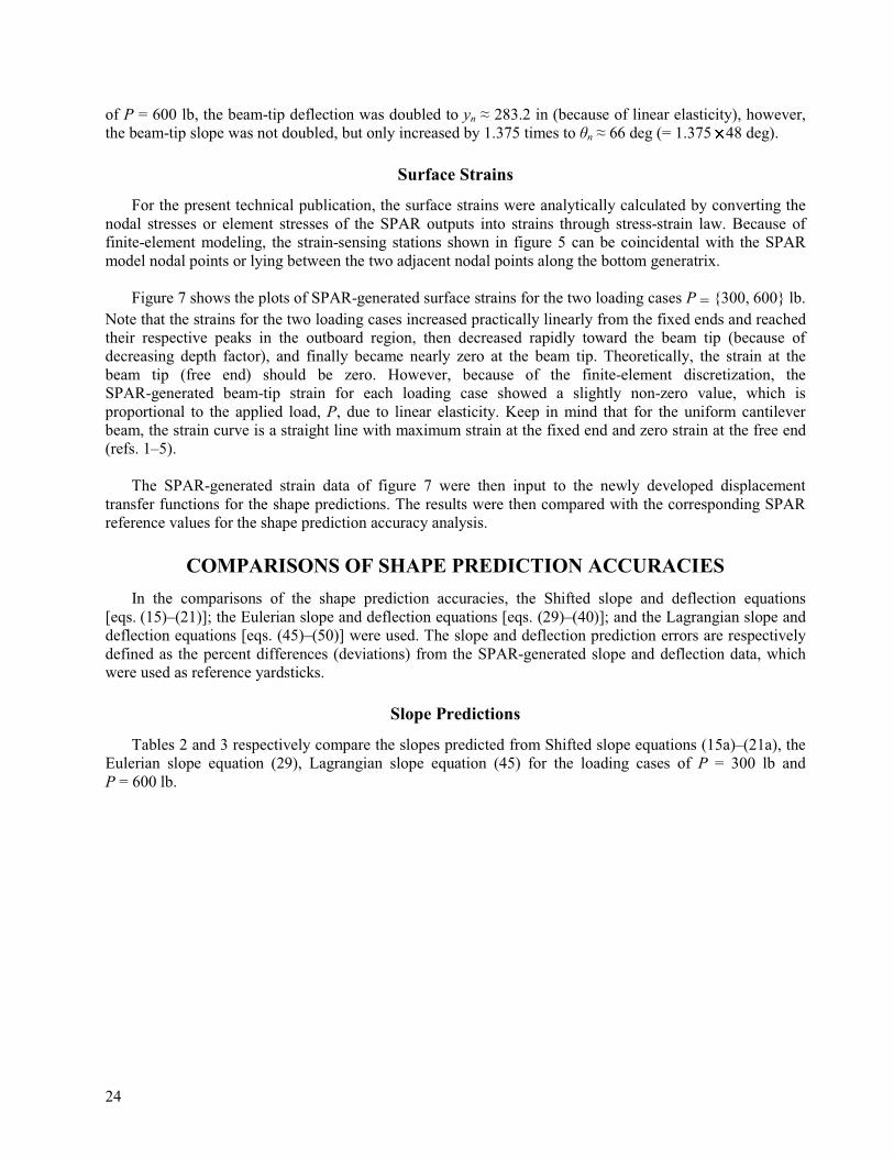
24

of P = 600 lb, the beam-tip deflection was doubled to yn 283.2 in (because of linear elasticity), however, the beam-tip slope was not doubled, but only increased by 1.375 times to �n �� deg (= 1.375 48 deg).

Surface Strains

For the present technical publication, the surface strains were analytically calculated by converting the nodal stresses or element stresses of the SPAR outputs into strains through stress-strain law. Because of finite-element modeling, the strain-sensing stations shown in figure 5 can be coincidental with the SPAR model nodal points or lying between the two adjacent nodal points along the bottom generatrix.

Figure 7 shows the plots of SPAR-generated surface strains for the two loading cases P = {300, 600} lb. Note that the strains for the two loading cases increased practically linearly from the fixed ends and reached their respective peaks in the outboard region, then decreased rapidly toward the beam tip (because of decreasing depth factor), and finally became nearly zero at the beam tip. Theoretically, the strain at the beam tip (free end) should be zero. However, because of the finite-element discretization, the SPAR-generated beam-tip strain for each loading case showed a slightly non-zero value, which is proportional to the applied load, P, due to linear elasticity. Keep in mind that for the uniform cantilever beam, the strain curve is a straight line with maximum strain at the fixed end and zero strain at the free end (refs. 1–5).

The SPAR-generated strain data of figure 7 were then input to the newly developed displacement transfer functions for the shape predictions. The results were then compared with the corresponding SPAR reference values for the shape prediction accuracy analysis.

COMPARISONS OF SHAPE PREDICTION ACCURACIESIn the comparisons of the shape prediction accuracies, the Shifted slope and deflection equations

[eqs. (15)–(21)]; the Eulerian slope and deflection equations [eqs. (29)–(40)]; and the Lagrangian slope and deflection equations [eqs. (45)–(50)] were used. The slope and deflection prediction errors are respectively defined as the percent differences (deviations) from the SPAR-generated slope and deflection data, which were used as reference yardsticks.

Slope Predictions

Tables 2 and 3 respectively compare the slopes predicted from Shifted slope equations (15a)–(21a), the Eulerian slope equation (29), Lagrangian slope equation (45) for the loading cases of P = 300 lb and P = 600 lb.

25

Table 2. Comparisons of slopes calculated from SPAR and from different slope equations; long tapered tube ( = 300 in, 0c = 4 in, nc = 1 in) subjected to tip load of P = 300 lb; n = 16; �l = 18.75 in.

Slope, deg �0 �2 �4 �6 �8 �10 �12 �14 �16(% diff.) (% diff.) (% diff.) (% diff.) (% diff.) (% diff.) (% diff.) (% diff.) (% diff.)

SPAR (reference)

0.0000 4.3526 9.4255 15.299 21.9903 29.3683 37.0656 44.2216 48.2679(0.0000) (0.0000) (0.0000) (0.0000) (0.0000) (0.0000) (0.0000) (0.0000) (0.0000)

Based on Shifted curvature equation (11)Non-

uniformeq. (15a)

0.0000 4.3461 9.4213 15.2919 21.9831 29.3545 37.0367 44.1651 48.0961

(0.0000) (0.1493) (0.0466) (0.0523) (0.0327) (0.0470) (0.0780) (0.1278) (0.3559)Slightly tapered

eq. (16a)

0.0000 4.3405 9.4084 15.2690 21.9481 29.3059 36.9773 44.1141 48.1723

(0.0000) (0.2780) (0.1814) (0.2020) (0.1919) (0.2125) (0.2382) (0.2431) (0.1981)

1st order eq. (17a)

0.0000 4.3426 9.4131 15.2771 21.9594 29.3191 36.9864 44.0967 48.0164

(0.0000) (0.2297) (0.1316) (0.1433) (0.1405) (0.1675) (0.2137) (0.2824) (0.5211)

2nd order eq. (18a)

0.0000 4.3459 9.4210 15.2912 21.9820 29.3526 37.0337 44.1603 48.0899

(0.0000) (0.1539) (0.0477) (0.0569) (0.0377) (0.0535) (0.0861) (0.1386) (0.3688)

Improvedeq. (19a)

0.0000 4.3447 9.4201 15.2903 21.9837 29.3607 37.0588 44.2497 48.2910

(0.0000) (0.1815) (0.0573) (0.0627) (0.0300) (0.0259) (0.0183) (0.0635) (0.0479)Log-

expanded eq. (20a)

0.0000 4.3444 9.4196 15.2892 21.9822 29.3590 37.0582 44.2597 48.3375

(0.0000) (0.1884) (0.0626) (0.0699) (0.0368) (0.0317) (0.0200) (0.0862) (0.1442)Depth-

expanded eq. (21a)

0.0000 4.3446 9.4198 15.2897 21.9826 29.3589 37.0560 44.2461 48.2888

(0.0000) (0.1838) (0.0605) (0.0667) (0.0350) (0.0320) (0.0259) (0.0544) (0.0433)*Based on Eulerian curvature equation (3)

Eulerian non-

uniformeq. (29)

0.0000 4.3544 9.5072 15.6656 23.1294 32.2247 43.2335 55.6503 63.8446

(0.0000) (0.0414) (0.8668) (2.3902) (5.1800) (9.7261) (16.6405) (25.8442) (32.2713)

Lagrangiannon-

uniformeq. (45)

0.0000 4.3419 9.3789 15.1108 21.4453 28.0683 34.4098 39.5432 41.9122(0.0000) (0.2458) (0.4944) (1.2360) (2.4784) (4.4265) (7.1651) (10.5794) (13.1679)^

26

Table 3. Comparisons of slopes calculated from SPAR and from different slope equations; long tapered tube( = 300 in, 0c = 4 in, nc = 1 in) subjected to tip load of P = 600 lb; n = 16; �l = 18.75 in.

Slope, deg(% diff.) (% diff.) (% diff.) (% diff.) (% diff.) (% diff.) (% diff.) (% diff.) (% diff.)

SPAR(reference)

0.0000(0.0000)

8.6553(0.0000)

18.3669(0.0000)

28.6842(0.0000)

38.9263(0.0000)

48.3787(0.0000)

56.4976(0.0000)

62.8071(0.0000)

65.9637(0.0000)

Based on Shifted curvature equation (11)Non-

uniformeq. (15a)

0.0000(0.0000)

8.6426(0.1467)

18.3691(0.0120)

28.6713(0.0450)

38.9162(0.0259)

48.3626(0.0333)

56.4700(0.0489)

62.7611(0.0732)

65.8349(0.1953)

Slightlytapered

eq. (16a)

0.0000(0.0000)

8.6319(0.2704)

18.3351(0.1731)

28.6335(0.1768)

38.8669(0.1526)

48.3061(0.1501)

56.4131(0.1496)

62.7196(0.1393)

65.8921(0.1085)

1st ordereq. (17a)

0.0000(0.0000)

8.6360(0.2230

18.3439(0.1252)

28.6468(0.1304)

38.8829(0.1115)

48.3215(0.1182)

56.4218(0.1342)

62.7054(0.1619)

65.7749(0.2862)

2nd ordereq. (18a)

0.0000(0.0000)

8.6424(0.1490)

18.3585(0.0457)

28.6703(0.0485)

38.9147(0.0298)

48.3605(0.0376)

56.4672(0.0538)

62.7572(0.0794)

65.8303(0.2022)

Improvedeq. (19a)

0.0000(0.0000)

8.6400(0.1768)

18.3569(0.0544)

28.6686(0.0544)

38.9171(0.0236)

48.3698(0.0184)

56.4911(0.0115)

62.8300(0.0365)

65.9811(0.0264)

Log-expandedeq. (20a)

0.0000(0.0000)

8.6394(0.1837)

18.3559(0.0599)

28.6669(0.0603)

38.9150(0.0290)

48.3678(0.0225)

56.4907(0.0122)

62.8381(0.0494)

66.0159(0.0791)

Depth-expandedeq. (21a)

0.0000(0.0000)

8.6397(0.1802)

18.3563(0.0577)

28.6676(0.0579)

38.9156(0.0275)

48.3678(0.0225)

56.4885(0.0161)

62.8271(0.0318)

65.9795(0.0240)*

Based on Eulerian curvature equation (3)Eulerian

non-uniformeq. (29)

0.0000(0.0000)

8.7088(0.6181)

19.0144(3.5254)

31.3314(9.2288)

46.2593(18.8382)

64.4514(33.2227)

86.4839(53.0754)

86.2696(37.3564)

88.1214(33.5907)

Based on Lagrangian curvature equation (7)Lagrangian

non-uniformeq. (45)

0.0000(0.0000)

8.6099(0.2461)

18.0458(1.7483)

27.4737(4.2201)

35.8469(7.9108)

42.0569(13.0673)

44.9455(20.4471)

44.9390(28.4492)

44.9879(31.7990)^

|<---------Acceptable range----------->|�--------------------------------Poor range-------------------------------------------->|* Most accurate at beam tip ^ Worst case

Note from tables 2 and 3 that the slope data predicted from the Shifted slope equations (15a) – (20a) are amazingly accurate beyond expectation. For the loading case of P = 300 lb (table 2), the beam-tip slope prediction errors are in the negligible range of 0.0433 to 0.5211 percent, and for the loading case of P = 600 lb (table 3), the beam-tip slope prediction errors decreased to the range of 0.0240 to 0.2862 percent(a nearly 45 percent reduction). The Depth-expanded slope equation (21a) produced the most accurate beam-tip slope data with infinitesimal prediction errors of only {0.0433, 0.0240} percent respectively for the loading cases of P = 300 lb (table 2) and P = 600 lb (table 3).

In tables 2 and 3, the slopes calculated from the Eulerian slope equation (29) are referred to the deformed x-coordinate and are therefore somewhat larger than the corresponding SPAR slopes, which are referred to the un-deformed x-coordinate [that is, )()( xs �� * , (fig. 2)]. The numbers listed in the parentheses under the slope data based on Eulerian formulation do not represent prediction errors, but are the percent differences because two different x-systems were used. When the load was doubled from P = 300 lb to P = 600 lb, the percent slope differences at the beam-tip based on Eulerian formulation increased from 32.2713 to 33.5907 percent (a nearly 4 percent increase).

27

The Lagrangian slope equation (45) predicted acceptable slope data in the inboard region, but the predicted slopes became lower than the corresponding SPAR reference slopes in the outboard region. When the load was doubled from P = 300 lb to P = 600 lb, the percent slope differences (errors) based on Lagrangian formulation increased from 13.1676 to 31.7990 percent (a nearly 141 percent increase) at the beam tip.

Slope Curves

The slope data listed in tables 2 and 3 are plotted in figures 8 and 9 respectively for the loading cases of P = {300, 600} lb for visual comparisons of the slope curves based on different formulations. As shown in figures 8 and 9, the slope curves based on the Shifted formulation [eqs. (15a) –(21a)] almost formed a single curve, which practically fell on top of the corresponding SPAR reference slope curve for the two loading cases P = {300, 600} lb, showing the high degrees of accuracies of the Shifted slope equations (15a)–(21a).

In figure 8 (loading case, P = 300 lb), the slope curve of Eulerian formulation [eq. (29)] practically lies on top of the SPAR reference slope curve only in the inboard region, but branched out upward away from the SPAR reference slope curve in the outboard region because SPAR slopes are based on the undeformed x-system. Keep in mind that the Eulerian slopes [ ] are always larger than the corresponding Lagrangian slopes [ )(x� ] [that is, )()( xs �� * , (fig. 2)].

The slope curve of Lagrangian formulation [eq. (45)] is quite close to the SPAR reference slope curve only in the inboard region, but branched out downward slightly away from the SPAR reference slope curve in the outboard region (fig. 8).

In figure 9 (loading case, P = 600 lb), the slope curve based on the Eulerian formulation [eq. (29)], except for a small inboard region, continued to deviate upward further away from the SPAR reference slope curve in the outboard region. Keep in mind that the Eulerian slopes [ ] are always larger than the corresponding Lagrangian slopes [ )(x� ] [that is, )()( xs �� * , (fig. 2)].The peculiar wavy behavior of the Eulerian slope curve near the beam tip region could be attributed to the mathematical functional behaviors of equations (29) and (24) at large slopes approaching 90 deg (table 3) as a result of the magnified effect of the term 2)/( dxdy .

At increasing load, P = 600 lb (fig. 9), the slope curve based on the Lagrangian formulation [eq. (45)], except for the small inboard region, deviated downward further away from the SPAR reference slope curve in the outboard region, causing the slope prediction errors to be greatly magnified. The rather poor slope predictions at increasing load (increasing deflections) could be attributed to the intensified effect of the term

2)/( dxdy in the Lagrangian curvature equation (7).

Deflection Predictions

Tables 4 and 5 respectively compare the deflections calculated from the Shifted deflection equations (15b, c)–(21b, c), from the Eulerian deflection equation (40), and from Lagrangian deflection equation (50), for the loading cases of P = 300 lb and P = 600 lb.

28

Table 4. Comparisons of deflections calculated from SPAR and from different deflection equations; long tapered tube ( = 300 in, 0c = 4 in, nc = 1 in) subjected to tip load of P = 300 lb; n = 16; �l = 18.75 in.

Deflection, in.

y0(% diff.)

y2(% diff.)

y4(% diff.)

y6(% diff.)

y8(% diff.)

y10(% diff.)

y12(% diff.)

y14(% diff.)

y16(% diff.)

SPAR(reference)

0.0000(0.0000)

1.4029(0.0000)

5.8910(0.0000)

14.0737(0.0000)

26.6907(0.0000)

44.7190(0.0000)

69.3198(0.0000)

101.7093(0.0000)

141.6016(0.0000)

Based on Shifted curvature equation (11)Non-uniformeq. (15b, c)

0.0000(0.0000)

1.3871(1.1262)

5.8746(0.2784)

14.0501(0.1667)

26.6660(0.0925)

44.6814(0.0841)

69.2690(0.0733)

101.6065(0.1011)

141.3056(0.2090)

Slightlytapered

eq. (16b, c)

0.0000(0.0000)

1.3859(1.2118)

5.8679(0.3921)

14.0321(0.2956)

26.6282(0.2342)

44.6117(0.2399)

69.1504(0.2444)

101.4226(0.2819)

141.1004 (0.3540)

1st ordereq. (17b, c)

0.0000(0.0000)

1.3863(1.1833)

5.8704(0.3497)

14.0387(0.2487)

26.6416(0.1840)

44.6348(0.1883)

69.1847(0.1949)

101.4585(0.2466)

141.0562 (0.3852)

2nd ordereq. (18b, c)

0.0000(0.0000)

1.3871(1.1262)

5.8744(0.2818)

14.0496(0.1712)

26.6650(0.0963)

44.6794(0.0886)

69.2649(0.0792)

101.5985(0.1089)

141.2901(0.2200)

Improvedeq. (19b, c)

0.0000(0.0000)

1.3865(1.1690)

5.8732(0.3022)

14.0476(0.1855)

26.6632(0.1030)

44.6810(0.0850)

69.2812(0.0557)

101.6760(0.0327)

141.5683(0.0235)*

Log-expanded

eq. (20b, c)

0.0000(0.0000)

1.3865(1.1690)

5.8731(0.3039)

14.0471(0.1890)

26.6620(0.1075)

44.6787(0.0901)

69.2772(0.0615)

101.6684(0.0402)

141.5643(0.0263)

Depth-expanded

eq. (21b, c)

0.0000(0.0000)

1.3865(1.1690)

5.8731(0.3039)

14.0472(0.1883)

26.6622(0.1068)

44.6789(0.0897)

69.2773(0.0613)

101.6686(0.0400)

141.5561(0.0321)


non-uniformeq. (40)

0.0000(0.0000)

1.3965(0.4562)

5.8862(0.0815)

14.0146(0.4199)

26.4191(1.0176)

43.7890(2.0797)

66.7253(3.7428)

95.3525(6.2500)

128.0932(9.5397)

Based on Lagrangian curvature equation (7)Lagrangiannon-uniform

eq. (50)

0.0000(0.0000)

1.3958(0.5061)

5.8823(0.1477)

14.0025(0.5059)

26.3874(1.1364)

43.7123(2.2512)

66.5437(4.0048)

94.9396(6.6559)

127.5099(9.9517)^

|<----------Acceptable range --------->|<--------------------------------Poor range-------------------------------------------->|* Most accurate at beam tip ^ Worst case

29

Table 5. Comparisons of deflections calculated from SPAR and from different deflection equations; long tapered tube ( = 300 in, 0c = 4 in, nc = 1 in) subjected to tip load of P = 600 lb; n ��l = 18.75 in.

Deflection, in.

y0(% diff.)

y2(% diff.)

y4(% diff.)

y6(% diff.)

y8(% diff.)

y10(% diff.)

y12(% diff.)

y14(% diff.)

y16(% diff.)

SPAR(reference)

0.0000(0.0000)

2.8058(0.0000)

11.7821(0.0000)

28.1474(0.0000)

53.3814(0.0000)

89.4380(0.0000)

138.6400(0.0000)

203.4154(0.0000)

283.2032(0.0000)

Based on Lagrangian curvature equation (11)Log-Non-uniform

eq. (15b, c)

0.0000(0.0000)

2.7742(1.1262)

11.7492(0.2792)

28.1001(0.1680)

53.3319(0.0927)

89.3628(0.0841)

138.5379(0.0736)

203.2131(0.0995)

282.6112(0.2090)

Slightlytapered

eq. (16b, c)

0.0000(0.0000)

2.7717(1.2153)

11.7359(0.3921)

28.0643(0.2952)

53.2565(0.2340)

89.2234(0.2399)

138.3008(0.2447)

202.8453(0.2803)

282.2007(0.3540)

1st orderEq. (17b, c)

0.0000(0.0000)

2.7726(1.1833)

11.7409(0.3497)

28.0774(0.2487)

53.2832(0.1840)

89.2696(0.1883)

138.3694(0.1951)

202.9170(0.2450)

282.1124(0.3852)

2nd ordereq. (18b, c)

0.0000(0.0000)

2.7742(1.1262)

11.7489(0.2818)

28.0993(0.1709)

53.3300(0.0963)

89.3587(0.0887)

138.5299(0.0794)

203.1971(0.1073)

282.5803(0.2199)

Improvedeq. (19b, c)

0.0000(0.0000)

2.7731(1.1654)

11.7465(0.3022)

28.0952(0.1855)

53.3264(0.1030)

89.3619(0.0851)

138.5624(0.0560)

203.3521(0.0311)

283.1367(0.0235)*

Log-expanded

eq. (20b, c)

0.0000(0.0000)

2.7731(1.1654)

11.7462(0.3047)

28.0943(0.1886)

53.3240(0.1075)

89.3573(0.0902)

138.5543(0.0617)

203.3368(0.0386)

283.1285(0.0264)

Depth-expanded

eq. (21b, c)

0.0000(0.0000)

2.7730(1.1690)

11.7462(0.3047)

28.0944(0.1883)

53.3244(0.1068)

89.3579(0.0896)

138.5545(0.0617)

203.3372(0.0384)

283.1123(0.0321)


non-uniformeq. (40)

0.0000(0.0000)

2.79213(0.4887)

11.7129(0.5866)

27.6060(1.9232)

51.1125(4.2505)

82.4108(7.8571)

131.48615.1598)

130.7083(36.7442)

151.6729(46.4438)^

Based on Lagrangian curvature equation (7)Lagrangiannon-uniform

eq. (50)

0.0000(0.0000)

2.7865(0.6879)

11.6815(0.8538)

27.5015(2.2947)

50.8036(4.8290)

81.3751(9.0151)

117.2992(15.3930)

154.5417(24.0265)

191.8715(32.2495)

|<----------Acceptable range---------->|<----------------------------------Poor range------------------------------------------>|* Most accurate at beam tip ^Worst case

Note from tables 4 and 5 that the deflections calculated from all the Shifted deflection equations (15b, c)–(21b, c) are amazingly accurate beyond expectations with negligible beam-tip prediction errors in the range of 0.0235 to 0.3852 percent for both loading cases, P = {300, 600} lb. Note also from tables 4 and 5 that under linear analysis, the predicted deflections and associated predicted deflection errors (in inch) arelinear functions of the applied load. Because of linearity, the deflection prediction errors (in percentage) are invariant to the loading magnitude. The improved deflection equations (19b, c) turned out to be the most accurate deflection equation, which produced only infinitesimal amount of prediction error of 0.0235 percent at the beam-tip for both loading cases, P = {300, 600} lb.

The Eulerian deflection equation (40) predicted acceptable deflection data in the inboard region, but the prediction errors continued to magnify toward the beam tip. Because the slope and deflections are not directly proportional to the surface strains in the Eulerian formulation [eqs. (34) and (40)], when the applied load, P = 300 lb, was doubled to P = 600 lb (surface strains doubled), the deflection prediction errors were greatly magnified from 9.5397 to 46.4438 percent (a nearly 387 percent increase) at the beam tip.

The Lagrangian deflection equation (50) also predicted acceptable deflection data in the inboard region, beyond which the prediction errors continue to magnify toward the beam tip. Because the slope and

30

deflections are not directly proportional to the surface strains in the Lagrangian formulation [eqs. (45) and(50)], when the applied load, P = 300 lb, was doubled to P = 600 lb, the deflection prediction errors increased nonlinearly from 9.9517 to 32.2495 percent (a nearly 224 percent increase) at the beam tip.

Deflection Curves

The deflection data listed in tables 4 and 5 are plotted in figures 10 and 11 respectively for the loading cases of P = {300, 600} lb for visual comparisons of the deflection curves based on different formulations.

As shown in figure 10 (loading case of P =300 lb), all the deflection curves based on the Shifted formulation [eqs. (15b, c)–(21b, c)] graphically fell on top of the associated SPAR reference deflection curves, showing exceptional accuracy of the Shifted deflection equations (15b, c)–(21b, c).

Note from figure 10 that for loading case of P = 300 lb, the deflection curves based on the Eulerian formulation [eq. (40)] and Lagrangian formulation [eq. (50)] are practically coincidental, and agreed with the SPAR reference deflection curve only in the inboard region, but deviated slightly downward from the SPAR reference deflection curve in the outboard region (fig. 10).

Figure 11 shows that at double load, P = 600 lb, the deflection curves based on the Shifted formulation [eqs. (15-b, c)–(21-b, c)] are again extremely close to the SPAR-reference deflection curve, showing amazing high degrees of prediction accuracies (tables 4, 5). The deflection curve of the Eulerian formulation agreed with the SPAR reference deflection curve only in the inboard region and deviated downward from the SPAR reference deflection curve in the outboard region, and became wavy near the beam tip, showing poor prediction performances. Again, the peculiar wavy behavior of the Eulerian deflection curve near the beam tip region is associated with the wavy behavior of the slope curve shown in figure 9, and could be attributed to the mathematical functional behaviors of equations (40) and (24) at large slopes approaching 90 deg (table 3).

As shown in figure 11, at doubled load P = 600 lb, the deflection curves based on the Lagrangianformulation [eq. (50)] fell on top of the SPAR reference deflection curve only in a small inboard region, and then branched out downward further away from the SPAR reference deflection curve toward the beam outboard region, giving discouraging shape predictions.

SHAPE PREDICTION ERROR CURVESThe slope and deflection predictions errors (percent differences from associated SPAR data) listed in the

parentheses in tables 2–5 are plotted in the following sections for visual comparisons.

Slope-Error Curves

Figure 12 shows the slope-error curves for P = 300 lb loading case associated with different Displacement Transfer Functions. The slope differential curve based on Eulerian formulation shown in figure 12 is not the slope error curve, but the curve showing the difference in slopes referred to the deformed and un-deformed x-coordinate. The slope differential for the Eulerian formulation steadily increased span-wisely and reached as large as 32.2713 percent at the beam tip (table 2).

The slope-prediction errors based on the Lagrangian formulation continued to increase almost linearly span-wisely and reached a peak value of 13.1676 percent at the beam tip (table 2).

31

The slope-error curves (fig. 12) based on the Shifted formulation practically formed a single curve along the 0 percent-error line and was indistinguishable; therefore, those slope error curves had to be re-plotted independently with a different scale.

Figure 13 shows the slope-error curves for the P = 300 lb loading case, calculated from seven Shifted slope equations (15a)–(21a). For the present example structure, the Depth-expanded case [eq. (21a)] produced the lowest slope-prediction errors near the beam tip region, with a slope prediction error of merely 0.0433 percent at the beam tip (table 2).

Figure 14 shows the slope-error curves for the P = 600 lb loading case associated with nine different displacement transfer functions. The lofty curve of the Eulerian formulation shown in figure 14 is not the slope-error curve, but a slope-differential curve for showing the difference in slopes based on the deformed x-coordinate (Eulerian) and un-deformed x-coordinate (SPAR). The peak slope differential of 53.0754 percent occurred at the strain-sensing station i =12 (table 3).

The slope-error curve of the Lagrangian formulation (fig. 12) is slightly s-shaped and tilted away from the 0 percent-error axis with peak error of 31.7990 percent at the beam tip (table 3). The seven slope-error curves based on the Shifted formulation (fig. 14) are crowded together near the 0 percent-error axis and practically indistinguishable. Therefore, for better visual comparisons, those seven slope-error curves based on the seven Shifted formulations had to be re-plotted with a different scale.

Figure 15 shows the slope-error curves for the P = 600 lb loading case calculated from the seven Shifted slope equations (15a)–(21a). For the present example structure, the Depth-expanded case [eq. (21a)] produced the lowest slope-error of 0.0240 percent at the beam tip ( table 3). Because the beam slopes are not directly proportional to the applied load, increasing the load from P = 300 lb to P = 600 lb caused the overall beam tip slope errors to come down by nearly 50 percent (compare figures 13 and 15).

Deflection-Error Curves

Figure 16 shows the deflection-error curves for the P = 300 lb loading case associated with ninedifferent displacement transfer functions. Note that both the Eulerian and Lagrangian formulations produced similar concave upward deflection-error curves lying far above the 0 percent-error axis, with respective deflection prediction errors as large as {9.5397, 9.9517}percent at the beam tip (table 4). Because the deflection-error curves based on the Shifted formulation are so close to the 0 percent-error axis, and are almost indistinguishable in figure 16, those deflection-error curves were re-plotted with a different scale for better visual comparisons.

Figure 17 shows the deflection-error curves for the P = 300 lb loading case, calculated from the seven sets of the Shifted deflection equations. (15b, c)–(21b, c)]. For the present example structure, the Improved case [eq. (19b, c)] produced the lowest deflection-prediction errors in the outboard region, with negligible deflection-prediction error of 0.0235 percent at the beam tip (table 4). The increasing deflection errors at strain-sensing station, i = 2, is due to a small predicted deflection error divided by a small SPAR reference deflection.

Figure 18 shows the deflection-error curves for the P = 600 lb loading case associated with ninedifferent displacement transfer functions. The deflection errors based on the Shifted formulation are very small as compared to those of both the Eulerian and Lagrangian formulations. The dent in the Eulerian deflection-error curve (fig. 18) is associated with the hump in the Eulerian slope-error curve (fig. 12). Because the deflection-error curves based on the Shifted formulation are so close and are almost indistinguishable in figure 18, those deflection-error curves were re-plotted using an enlarged scale for better visual comparisons.

32

Figure 19 shows the deflection-error curves for the P = 600 lb loading case calculated from the seven sets of Shifted deflection equations (15b, c)–(21b, c). Because the beam deflections are directly proportional to the strains (or applied load), by increasing the load from P = 300 lb to P = 600 lb, the overall deflectionerrors remain practically the same (tables 4 and 5). Again, the increasing deflection errors at strain-sensing station, 2�i , is due to a small deflection error divided by a small SPAR reference deflection. For the present example structure, the Improved case [eq. (19b, c)] produced the lowest deflection errors in the outboard region, with a negligible deflection prediction error of 0.0235 percent at the beam tip (same as the P = 300 lb case) (that is, figs. 17 and 19 are practically identical).

EXPERIMENTAL VALIDATIONS OF SHAPE-PREDICTION ACCURACIES

In the process of writing the present technical publication, large-scale ground loads tests were conducted on a long span (high aspect ratio) full-scale tapered wing (175-ft wingspan) at the NASA Dryden FlightLoads Laboratory. These ground tests were used to validate the shape prediction accuracies of the Displacement Transfer Functions. The results were reported in a separate NASA technical publication authored by Jutte, Ko, et al (ref. 19).

In the ground tests, the whole wing was loaded from 0 percent up to 100 percent design limit load (DLL) at which the wing-tip slope exceeded 20 deg. Surfaces strains were measured by using four fiber-optic strain-sensing lines installed on the wing surfaces (two on the wing upper surface, two on the wing lower surface). Wing deflections were measured by means of a photogrammetry system, and were used as yardsticks to evaluate the accuracies of the predicted wing deflections. Using the measured surface strains as inputs, theoretical wing deflections were calculated from the recursive Displacement Transfer Functions [eqs. (16a, b)], which were formulated for slightly tapered beams (based on piecewise-linear strain representations) such as the current slightly tapered wing structure.

For completeness of the present technical report, wing deflection plots in figures 11, and 12 of reference 19 were duplicated respectively as figures 20, and 21 in the present technical report. Figures 20, and 21respectively show the plots of the predicted and experimentally measured wing deflections along the number 3 (FWD) and number 4 (AFT) strain-sensing lines. Amazingly, the measured data points practically fell on top of the associated predicted deflection curves for the whole range of loading levels [(0~100) percent DLL]. The wing-tip prediction errors associated with the number 3 and number 4strain-sensing lines are respectively in the negligible ranges of (0.09~1.72) percent and (0.25~1.45) percentat 100 percent DLL depending on the sensor-to-sensor distances used. For details of the experimental shape-prediction studies, please see reference 19.

Note from figures 20 and 21 that the maximum wing-tip deflections of the Global Observer reached approximately 160 in. Hence, the ratio of (maximum wing-tip deflection) to (half wingspan) can be calculated as:

0.1524 = 15.24% (51)

The 15.24 percent normalized wing-tip deflection from equation (51) indicates that the ground test of the Global Observer was operating in a borderline region between the linear and nonlinear regimes.

Keep in mind that each Shifted Displacement Transfer Function was formulated by geometrically relating the surface strains to curvatures, and then to deflections. Therefore, one could expect that the Shifted Displacement Transfer Function can faithfully compute the right deflections whether the input

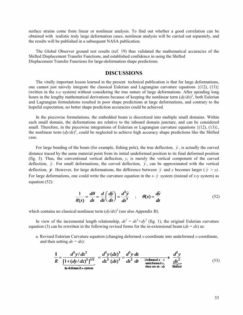
33

surface strains come from linear or nonlinear analysis. To find out whether a good correlation can be obtained with realistic truly large deformation cases, nonlinear analysis will be carried out separately, and the results will be published in a subsequent NASA publication.

The Global Observer ground test results (ref. 19) thus validated the mathematical accuracies of the Shifted Displacement Transfer Functions, and established confidence in using the Shifted Displacement Transfer Functions for large-deformation shape predictions.

DISCUSSIONSThe vitally important lesson learned in the present technical publication is that for large deformations,

one cannot just naively integrate the classical Eulerian and Lagrangian curvature equations {(12), (13)} (written in the x-y system) without considering the true nature of large deformations. After spending long hours in the lengthy mathematical derivations because of keeping the nonlinear term (dy/dx)2, both Eulerian and Lagrangian formulations resulted in poor shape predictions at large deformations, and contrary to thehopeful expectation, no better shape prediction accuracies could be achieved.

In the piecewise formulations, the embedded beam is discretized into multiple small domains. Within each small domain, the deformations are relative to the inboard domain juncture, and can be considered small. Therefore, in the piecewise integrations of Eulerian or Lagrangian curvature equations {(12), (13)},the nonlinear term (dy/dx)2, could be neglected to achieve high accuracy shape predictions like the Shiftedcase.

For large bending of the beam (for example, fishing pole), the true deflection, y� , is actually the curved distance traced by the same material point from its initial undeformed position to its final deformed position (fig. 3). Thus, the conventional vertical deflection, y, is merely the vertical component of the curved deflection, y� . For small deformations, the curved deflection, y� , can be approximated with the vertical deflection, . However, for large deformations, the difference between y� and y becomes larger ( y� > y).For large deformations, one could write the curvature equation in the s- y� system (instead of x-y system) asequation (52):

; (52)

which contains no classical nonlinear term (dy/dx)2 (see also Appendix B).

In view of the incremental length relationship, ds2 = dx2+dy2 (fig. 1), the original Eulerian curvature equation (3) can be rewritten in the following revised forms for the in-extensional beam (ds = dx) as:

a. Revised Eulerian Curvature equation (changing deformed x-coordinate into undeformed x-coordinate, and then setting ds = dx):

(53)

34

Also, in view of the incremental length relationship, ds2 = (dx–du)2 + dy2 (fig. 2), the original Lagrangian curvature equation (4) can be rewritten in the following revised forms for the in-extensional beam (ds = dx) as:

b. Revised Lagrangian curvature equation (setting du = 0, ds = dx)

(54)

Note that, for the in-extensional beams (ds = dx), both equations (53) and (54), written in undeformedx-system (x = s), degenerated into the Shifted curvature equation (11), containing no nonlinear term(dy / dx)2. Thus, the formulations based on the revised Eulerian and Lagrangian curvature equations {(53) or (54)}, become the Shifted formulation, and can provide accurate shape predictions.

CONCLUDING REMARKSLarge-Deformation Displacement Transfer Functions were formulated through piecewise integrations of

the Eulerian curvature-strain equation, the Lagrangian curvature-strain equation, and the Shifted curvature-strain equation. A long tapered cantilever tubular beam was chosen in the shape-prediction accuracy studies of the newly developed Displacement Transfer Functions. Surface strains for input to the Displacement Transfer Functions were analytically calculated from the finite-element analysis of the taperedcantilever tubular beam. Also, the finite-element-generated slopes and deflections were used as reference yardsticks in the prediction accuracy studies. The results are itemized below:

1. Changing from piecewise-linear strain representations to piecewise-nonlinear strain representations, the shape prediction accuracies could be improved considerably for the tapered cantilever tubular beam.

2. Based on the Shifted curvature equation, the resulting seven sets of the Shifted Displacement Transfer Functions were found to be amazingly accurate beyond expectation for large-deformation shape predictions, even for the case with a beam-tip slope reaching as large as 66 deg. The beam-tip shape prediction errors of the seven sets of the Shifted slope and deflection equations, are in the negligible ranges of {0.0240 – 0.5211} percent for the slopes, and {0.0235 – 0.3852} percent for the deflections.

3. For the Shifted formulation (based on linear analysis), the deflections are directly proportional to the surface strains, and therefore, for the same type of loading condition, the negligible deflection prediction errors are theoretically independent of the loading magnitude (that is, degree of deformation).

4. The amazing accuracy of the Shifted formulation could be attributed to: 1) shifting of the deformed material points back to their respective initial undeformed x-positions; and 2) piecewise integrations of the Shifted curvature equation, enabled by dicretization of the embedded beam.

5. Based on the classical Eulerarian curvature equation, the resulting slope and deflection equations gave poor shape predictions at large deformations because of retaining the term (dy / dx)2 in the discretized approach. The beam tip deflection prediction errors are in the poor ranges of {9.5397 – 46.4438} percent.

35

6. Based on Eulerian formulation, when the applied load was doubled (that is, doubling deflections), because the deflections are not directly proportional to the surface strains, the deflection prediction errors were greatly magnified from 9.5397 percent to 46.4438 percent at the beam-tip (a 386.8476 percentincrease).

7. Based on the physical (Lagrangian) curvature equation, the resulting slope and deflection equations gave discouraging shape predictions at large deformations because of retaining the term (dy / dx)2 in the discretized approach. The beam-tip prediction errors are in the poor range of {13.1676 – 31.7990} percentfor the slopes, and {9.9517 – 32.2495} percent for the deflections.

8. Based on the Lagrangian formulation, when the applied load was doubled (that is, doubling deflections), because the slopes and deflections are not directly proportional to the surface strains, the beam-tip slope prediction errors were magnified from 13.1676 percent to 31.7990 percent (a 141.4943percent increase), and the beam-tip deflection prediction errors increased from 9.9517 percent to 32.2485percent (a 224.0602 percent increase).

9. If the deformed material points of an in-extensional beam are shifted back to their respective initial undeformed x-locations, then the term (dy / dx)2 in the Lagrangian curvature equation will become zero, implying linearization. The resulting linearlized Lagrangian formulation will become the Shifted formulation, and provides equally accurate shape predictions.

10. The linearized Eulerian curvature equation [the term (dy / dx)2 neglected], even with similar mathematical form, cannot be equivalent to the Shifted curvature equation because, the former is referred to the deformed x-coordinate, while the latter to the undeformed x-coordinate. The two x-systems will become quite different at large deformations.

11. The simplified alternative deflection equations developed for the Eulerian and Lagrangianformulations could not provide good shape predictions at large deformations because of the poor input slope data at large deformations.

12. Retaining the term (dy / dx)2 in the piecewise integrations of curvature equations resulted in rather poor shape prediction performances of both the Eulerian and Lagrangian formulations.

13. For in-extensional beams (ds = dx), by writing the original Eulerian and Lagrangian curvatureequations in s-system, the formulations based on the revised Eulerian and Lagrangian curvature equationscan degenerate into the Shifted formulation and, therefore, could provide accurate shape predictions.

14. The Global Observer ground test results validated the mathematical accuracies of the Shifted Displacement Transfer Functions formulated, and giving confidence in using the Displacement Transfer Functions for large-deformation shape predictions.

36

FIGURES

Figure 1. Small segment of the deformed nonuniform embedded beam for geometrically relating local radius of curvature, R(s), to associated surface bending strain.

Figure 2. Small segment of the deformed-beam elastic curve used for deriving the physical (Lagrangian) curvature equation.

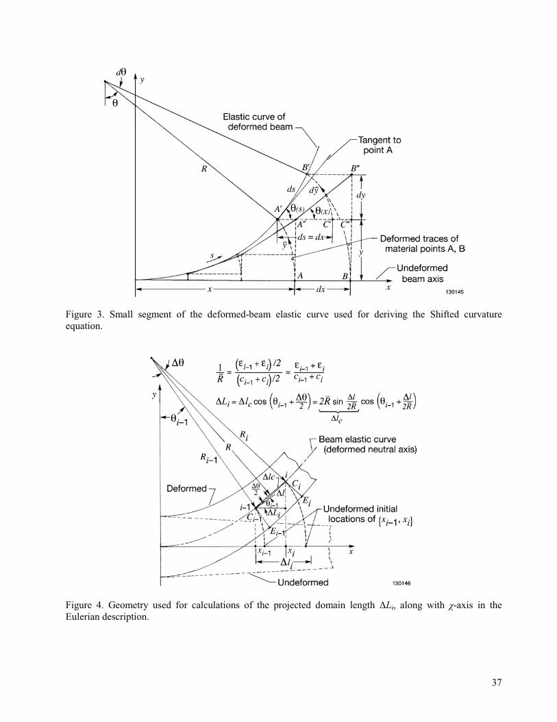
37

Figure 3. Small segment of the deformed-beam elastic curve used for deriving the Shifted curvature equation.

�� !�� " #"�# �� !� �� $��&�"�� #�� Li, along with �-axis in the Eulerian description.

38

Figure 5. Tapered cantilever tubular beam with strain-sensing stations evenly distributed along the bottom strain-sensing line.

Figure 6. Large deformation of the tapered cantilever tubular beam (SPAR finite-element model) subjected to a vertical tip load of P = 300 lb (or P = 600 lb); l = 300 in; c0 = 4 in; cn = 1 in.

39

Figure 7. SPAR-generated surface-strain curves for the tapered cantilever tubular beam subjected to tip loads of P = {300,600} lb; l = 300 in; c0 = 1 in.

Figure 8. Slopes of the tapered cantilever tubular beam calculated from slope equations based on the Eulerian, Lagrangian, and Shifted formulations; l = 300 in; c0 = 4 in; cn = 1 in; P = 300 lb.

40

Figure 9. Slopes of the tapered cantilever tubular beam calculated from slope equations based on theEularian, Lagrangian, and Shifted formulations; l = 300 in; c0 = 4 in; cn = 1 in; P = 600 lb.

Figure 10. Deflections of the tapered cantilever tubular beam calculated from deflection equations based on the Eularian, Lagrangian, and Shifted formulations; l = 300 in; c0 = 4 in; cn = 1 in; P = 300 lb.

41

Figure 11. Deflections of the tapered cantilever tubular beam calculated from deflection equations based on the Eulerian, Lagrangian, and Shifted formulations; l = 300 in; c0 = 4 in; cn = 1 in; P = 600 lb.

Figure 12. Comparisons of �i prediction errors of different displacement transfer functions; long tapered cantilever tubular beam; l = 300 in; c0 = 4 in; cn = 1 in; P = 300 lb at tip.

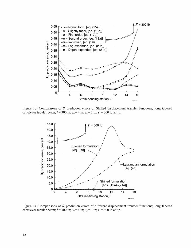
42

Figure 13. Comparisons of �i prediction errors of Shifted displacement transfer functions; long tapered cantilever tubular beam; l = 300 in; c0 = 4 in; cn = 1 in; P = 300 lb at tip.

Figure 14. Comparisons of �i prediction errors of different displacement transfer functions; long tapered cantilever tubular beam; l = 300 in; c0 = 4 in; cn = 1 in; P = 600 lb at tip.

43

Figure 15. Comparisons of �i prediction errors of Shifted displacement transfer functions; long tapered cantilever tubular beam, l = 300 in; c0 = 4 in; cn = 1 in; P = 600 lb at tip.

Figure 16. Comparisons of yi prediction errors of different displacement transfer functions; long tapered cantilever tubular beam; l = 300 in; c0 = 4 in; cn = 1 in; P = 300 lb at tip.

44

Figure 17. Comparisons of yi predicition errors of Shifted displacement transfer functions; long tapered cantilever tubular beam; l = 300 in; c0 = 4 in; cn = 1 in; P = 300 lb at tip.

Figure 18. Comparisons of yi prediction errors of different displacement transfer functions; long tapered cantilever tubular beam; l = 300 in; c0 = 4 in; cn = 1 in; P = 600 lb at tip.

45

Figure 19. Comparisons of yi prediction errors of Shifted displacement transfer functions; long tapered cantilever tubular beam; l = 300 in; c0 = 4 in; cn = 1 in; P = 600 lb at tip.

Figure 20. Comparison of predicted and measured wing deflections along the number 3 strain-sensing line for different loading levels (duplication of figure 11, ref. 18).

46

Figure 21. Comparison of predicted and measured wing deflections along the number 4 strain-sensing line for different loading levels (duplication of figure 12, ref.18).

47

APPENDIX A

ALTERNATIVE DERIVATION OF THE PHYSICAL (LAGRANGIAN)CURVATURE EQUATION

The alternative method used by Kopmaz, et al (ref. 12) and Hodges (ref. 13) in deriving the physical (Lagrangian) curvature equation (7) is described in the following paragraphs.

In view of figure 2, when the beam is bent, the undeformed material points, )0,({ xA , )}0,( dxxB � , will be moved to respective deformed positions, ]),[({ yuxA �� , )]}(),()[( dyyduudxxB �� , in which {u,y} respectively denote the horizontal and vertical displacement of material point A (moving to point ). Then, in view of the curved triangle CBA �� , the infinitesimal curved length, )( BAds �� , along the elastic curve of the deformed beam can be expressed in terms of {dx, du, dy} as:

22 )()( dydudxds �� (A1)

Dividing through equation (A1) by dx , one obtains equation (A2):

22

1 ��

��

��

��

dxdy

dxdu

dxds (A2)

In view of curved triangle CBA �� (fig. 2), the slope, )(tan s� , at point A� can be expressed as equation (A3):

dxdudxdy

dudxdys

/1/)(tan

��

�� (A3)

from which, one obtains equation (A4):

��

��

��

dxdudxdys/1

/tan)( 1� (A4)

Differentiating equation (A-4) with respect to x, one obtains equation (A5):

2

2

2222

/1/1

)/1()/)(/()/1)(/(

)(

��

��

��

��

�

dxdudxdydxdu

dxuddxdydxdudxyd

dxsd�

22

2

2

2

2

1

1

��

��

�

��

��

��

��

�

dxdy

dydu

dxud

dxdy

dxdu

dxyd

(A5)

The curvature, R/1 , of the elastic curve of the deformed beam can be written as:

dsdx

dxsd

dssd

R)()(1 ��

�� (A6)

48

Substitutions of equations (A2) and (A5) into equation (A6) yields equation (A7):

2322

2

2

2

2

/

22

/

22

2

2

2

2

1

1

1

1

1

11

��

�

��

��

��

��

��

��

��

�

��

��

��

��

��

��

��

��

��

��

�

dxdy

dxdu

dxud

dxdy

dxdu

dxyd

dxdy

dxdu

dxdy

dxdu

dxud

dxdy

dxdu

dxyd

R

dsdxdxd��

�

(A7)

For the in-extensional beam, the curved coordinate, s, of any deformed material point is always equal to its initial un-deformed x-coordinate (fig. 2). Namely, xs � and dxds � , and equation (A2) can be written as:

22

11 ��

��

��

��

dxdy

dxdu (A8)

Rearranging equation (A8) as equation (A9):

0222

��

��

��

��

dxdy

dxdu

dxdu (A9)

Solving for dxdu / one obtains:

2

11 ��

��+�

dxdy

dxdu (A10)

which can be rewritten as:

2

11 ��

��

dxdy

dxdu

� (A11)

Differentiating equation (A10), 22 / dxdu can be expressed as:

2

2

2

2

2

1 ��

��

�

dxdy

dxyd

dxdy

dxud

� (A12)

49

Substitutions of equations (A11) and (A12) into the curvature equation (A7) yields equation (A13):

22322

2

222

2

2

232

22

2

2

2

2

2

2

11

1

1

1

1

1

��

��

��

�

��

��

��

��

��

��

��

��

�

��

��

��

�

��

��

�

��

��

��

��

��

�

�

��

�

��

��

��

��

��

�

�

��

�

��

��

�

dxdy

dxdy

dxdy

dxyd

dxdy

dxdy

dxyd

dxdy

dxdy

dxdy

dxyd

dxdy

dxdy

dxdy

dxyd

R

��

�

��

(A13)

After cancelling terms, and choosing the positive sign, one obtains equation (A14):

$ %222

/1

/1

dxdy

dxydR �� (A14)

which is the physical (Lagrangian) curvature equation (7) for the in-extensional beam.

Keep in mind that dxdy / in equation (A14) is referred to the undeformed x-system. From right triangle, )( DEA�� (fig. 2), the slope, )(x� , in the x-system can be expressed as equation (A15):

��

��

dxdyx 1tan)(� (A15)

Comparing equations (A15) and (A4), one notes that )(x� in the undeformed x-system is slightly

smaller than in the s-system [that is, ] (fig. 2).

In the bending deformations, the axial displacement, u, of a material point is very small. If the axial displacement, u, is neglected (that is, 0 u ) in equation (A4), then )(s� will become )(x� of equation (A15). The condition ( 0 u ) implies that the deformed material points A�{ , }B� (fig. 3) are horizontally shifted back to points A ��{ , }B �� at their respective initial undeformed x-locations. It is important to mention that 0 u will make 0/ dxdy according to equation (A8).

50

APPENDIX B

GRAPHICAL DERIVATION OF THE SHIFTED CURVATURE EQUATIONFor the in-extensional beam, the curved coordinate, s, of any deformed material point is always equal to

its initial un-deformed coordinate x (fig. 3). Namely, and , then the basic curvature equation can be written as equation (B1):

(B1)

In the Eulerian or Lagrangian curvature equation (3) or (7), the term 2)/( dxdy appeared because, the slope, )(s� , of the beam elastic curve was expressed in term of either or )/(sin 1 dsdy� . It was found that term 2)/( dxdy caused the formulated Displacement Transfer Functions to give rather poor shape predictions at large deformations. To avoid the appearance of the term 2)/( dxdy , one can alternatively express the slope, )(s� , in term of the curved deflection, y� , (fig. 3), which is the curved length AA � actually traced by the same material point from its initial un-deformed position to its final deformed position . Thus, in view of the infinitesimal curved triangle, CBA �� [ C � will converge to

BB � -curve in the limit, 0 �d , (fig. 3)], the slope, )(s� , can then be expressed as:

(B2)

By combining equations (B1) and (B2), one obtains the following curvature equation (B3) associated with the curved deflection, y� , as:

(B3)

In the formulations of the Shifted displacement transfer functions, the deformed material points A�{ }B� (fig. 3) are shifted horizontally to points A ��{ , }B �� with x-coordinates respectively matching the

original un-deformed x-coordinates of points A{ , }B . The curve connecting the shifted deformed material points will be slightly detached from the true elastic curve of the actual deformed beam. Keep in mind that, in the bending deformations, the axial displacements are miniscule, and so also the amounts of horizontal shifting.

Graphically, the horizontal shifting (fig. 3) will cause the curved deflection, , to distort into a straight vertical deflection, y, and also causing the curved triangle, CBA �� , to distort into a right triangle, CBA �� .Thus, the shifted-slope, )]/(tan)[( 1 dxdyx �� , in the x-system will be slightly smaller than the original slope, )]/(sin)[( 1 dsdys �� in the s-system [that is, )()( sx �� & , (fig. 3)]. After the horizontal shifting, and ignoring the resulting small perturbation of R(x), equation (B-3) can be rewritten as equation (B-4):

(B4)

51

which is similar to equation (11) in the main text, and is called the Shifted curvature equation for the in-extensional beam .

52

APPENDIX C

DERIVATION OF PROJECTED DOMAIN LENGTH FOR THEEULERIAL FORMULATION

In view of curvature-strain equation (2), the averaged curvature, R/1 (fig. 4), for the elastic curve bounded by �� can be approximated by using the averaged strains and the averaged depth factor as equation (C1):

2/)(2/)(1

1

1

1

1

ii

ii

ii

ii

ccccR ��

��

��

�

�

� (C1)

In view of figure 4, for the in-extensional beam, one can relate the chord length, cl� , between points { 1�i , }i , to the curved domain length, l� , as:

RlRRlc 2

sin22

sin2 ��

��

� (C2)

The deformed domain length, iL� , [projection of cl� along the x-axis] can be obtained by taking cosine of the chord length, cl� [eq. (C-2)] as:

��

��

��

��

��

��

�

� Rl

RlRlL i

l

ici

c

2cos

2sin2

2cos 11 ��

��

),....,3,2,1( ni �

(C3)

Substitution of equations (C1) and (C2) into equation (C3) yields the deformed domain length, ,along the deformed x-axis as equation (C4):

��

��

��

��

��

��

��

��

��

��

��

�

�

�

�

ii

iii

ii

ii

ii

iii cc

lcc

lccL1

11

1

1

1

1

2cos

2sin2 �

),....,3,2,1( ni �

(C4)

which is equation (24) in the main text.

53

APPENDIX D

DERIVATIONS OF THE EULERIAN SLOPE EQUATIONS Equation (26) is reproduces as equation (D1) in the following:

; (D1)

On the left hand side of equation (D1), the lower limit of the integration, 1�iV , is defined as the value of V at 1�ix , namely, 111 tan)(tan)( �� iiii xxVV �� .

Integrations of both sides of equation (D1) yield (refs.1, 17,):

��

�

�

��

�

� ��

�

��

��

��

�

��

1

111

21

111111)()(

log)(

)()(

i

iii

ii

eii

iiiiiiiii c

cxxL

cc

ccccccL

)( 1 ii xxx ��

(D2)

After simplification, equation (D2) becomes equation (D3):

��

��

��

��

��

��

��

��

��

��

��

��

��

��

��

��

��

�

�

�

� 11log)(

)(1

1 1

12

1

111

1

121

12

i

i

i

ie

ii

iiiiii

ii

ii

i

i

Lxx

cc

ccccLxx

ccV

VVV

)( 1 ii xxx ��

(D3)

54

Squaring both sides and rearranging, and then taking the square root, the slope, )(tan)( xxV �� can be expressed as:

2

1

12

1

111

1

1

12

1

1

12

1

111

1

1

12

1

11log)(

)(tan1

tan1

11log)(

)(tan1

tan

)(tan

��

��

�

��

��

��

��

��

��

��

��

��

��

��

��

�

��

��

��

��

��

��

��

��

��

��

�

�

��

��

�

�

�

�

�

��

��

�

�

�

�

��

��

M

i

i

i

ie

ii

iiiiii

ii

ii

i

i

M

i

i

i

ie

ii

iiiiii

ii

ii

i

i

Lxx

cc

ccccLxx

cc

Lxx

cc

ccccLxx

ccx

�

�

�

�

�

)( 1 ii xxx ��

(D4)

At the deformed strain-sensing station, ixx � , we have iii Lxx �� )( 1 , and equation (D4) becomesequation (D5):

2

12

1

11

1

1

12

1

12

1

11

1

1

12

1

log)(tan1

tan1

log)(tan1

tan

tan

��

��

��

��

��

��

�

��

��

��

�

��

��

�

��

��

��

�

��

��

�

�

�

�

��

��

�

�

�

�

i

ie

ii

iiii

ii

iii

i

i

i

ie

ii

iiii

ii

iii

i

i

i

cc

cccc

ccL

cc

cccc

ccL

�

�

�

�

�

),....,3,2,1( ni �

(D5)

which is identical to the Eulerian slope equation (29) for large deformations of nonuniform beams (uniform beams excluded).

Log-Expanded Slope Equation

Note from equation (C4) that, the logarithmic terms and the denominators containing factor, )( 1�� ii cc ,will cause mathematical indeterminacy (that is, 0/0) for the uniform beam case )( 1 ccc ii �� . The way to bypass such a mathematical indeterminacy problem is to expand logarithmic function in series form in terms of )( 1�� ii cc . This approach enables the canceling out of the factor, )( 1�� ii cc , in the denominator of

equation (D4). Keep in mind that in equation (D4), the two conditions, 10 1 ��

� �

i

i

Lxx and

0111

&��

��

��&�

�i

i

cc , caused the required condition, 111 1

1&�

�

��

�

��

��

��

��&� �

� i

i

i

i

Lxx

cc , to hold for series

expansion of the logarithmic term, ��

��

��

��

��

��

��

�

11log 1

1 i

i

i

ie L

xxcc , expressed in terms of )( 1�� ii cc (ref. 17)

as:

55

��

��

��

��

��

��

��

�

11log 1

1 i

i

i

ie L

xxcc ....1

211

21

2

1

1

1��

�

��

��

��

��

��

��

��

��

��

�

�

� i

i

i

i

i

i

i

i

Lxx

cc

Lxx

cc

....21

21

2

1

11

1

1 ��

��

��

��

��

� ��

��

� �

�

��

�

�

i

i

i

ii

i

i

i

ii

Lxx

ccc

Lxx

ccc (D6)

In light of equation (D6), the term M in equation (D4) can be written as equation (D7):

��

��

��

��

��

��

��

��

��

� �

��

��

�

� 11log)(

)( 1

12

1

111

1

1

i

i

i

ie

ii

iiiiii

ii

ii

Lxx

cc

ccccLxx

ccM

�� termsexpanded-Log

21

2

1

11

1

12

1

111

1

1 ....21

)()(

��

�

��

��

��

��

��

��

� ��

��

��

��

� �

�

��

�

�

�

��

�

�

i

i

i

ii

i

i

i

ii

ii

iiiiii

ii

ii

Lxx

ccc

Lxx

ccc

ccccLxx

cc

....2

)()()(

)(2

12

1

111

11

111

1

1 ��

��

��

��

� �

�

��

��

��

�

�

i

i

i

iiiii

iii

iiiii

ii

ii

Lxx

cccxx

cccccxx

cc

��

��

��

��

��

��

�

��

��

� ....2

)()()(

)( 21

21

1111111

11

1

i

i

i

iiiiiiiiiiii

iii

i

Lxx

ccccccc

cccxx

��

��

��

��

��

��

�

��

��

� ....2

)()]([)(

)( 21

21

1111

11

1

i

i

i

iiiiiii

iii

i

Lxx

ccccc

cccxx (D7)

After canceling out the factor, )( 1 ii cc �� , the term M becomes:

��

��

��

��

��

�

��

�

� ....2

)()(2

12

1

111

1

1

i

i

i

iiiii

i

i

Lxx

cccxx

cM

(D8)

In view of equation (D8), the slope equation (D4) takes on the following form:

22

12

1

111

1

1

12

1

21

21

111

1

1

12

1

2)()(

tan1

tan1

2)()(

tan1

tan

)(tan

��

��

��

��

��

��

�

��

��

�

�

�

��

�

�

�

�

�

�

��

�

�

�

�

i

i

i

iiiii

i

i

i

i

i

i

i

iiiii

i

i

i

i

Lxx

cccxx

c

Lxx

cccxx

cx

�

�

�

�

�

)( 1 ii xxx ��

(D9)

56

At the deformed strain-sensing station, ixx � , we have iii Lxx �� )( 1 , and equation (D9) becomes:

2

21

11

1

1

12

1

21

11

1

1

12

1

2tan1

tan1

2tan1

tan

tan

��

��

��

��

��

�

��

��

�

��

�

�

�

�

�

��

�

�

�

�

i

i

iiiii

i

i

i

i

M

i

i

iiiii

i

i

i

i

i

Lc

ccLc

Lc

ccLc

�

�

�

�

�

��

),....,3,2,1( ni �

(D10)

The term M in equation (D10) can be further simplified as:

221

11

1

1 i

i

iiiii

i

i Lc

ccLc

M ��

�

��

�

�

��

��

� ��

��

�

��

�

��

�

�

21

1111

21

11

1

1

22

2

i

iiiiiii

i

iiiiii

i

i

ccccL

cccLL

c

��

��

��

�

��

��

��

��ii

i

i

i

i

cc

cL 1

112

2 (D11)

In view of equation (D11), equation (D10) takes on the final form as:

),....,3,2,1( ni �

(D12)

Equation (D12) is the log-expanded Eulerian slope equation (34) for large deformations of nonuniform beams including uniform beams as special cases.

57

APPENDIX E

DERIVATION OF THE LAGRANGIAN SLOPE EQUATIONEquation (42) is duplicated as equation (E1) in the following:

; (E1)

In equation (E1), )(tan/ xdxdyV �� , and the lower limit of integration, 1�iV , on the left hand side is the value of V at the strain-sensing station, 1�� ixx [that is, 11 )/( �� ii dxdyV )(tan 1�� ix� 1tan �� i� ]. Integrations of both sides of equation (E1) yield (refs. 1, 17):

111 sinsin �

�� iVV )()( 1

1

1�

�

� ��

� iii

ii xxcc

��

��

��

��

��

�

��

��

��

�

� ��

�

��

1111

2

21

1111

log)()(log

)()(

)()(

ieiiii

eii

iiiiii

ccxxl

cc

lcc

lcc

lc

)()( 1

1

1�

�

� ��

� iii

ii xxcc

��

�

�

��

�

� ��

�

��

��

��

�

��

1

111

21

1111)()(

log)(

)()(

i

iiii

eii

iiiiii

c

cxxl

cc

cccccl (E2)

After simplifications, equation (E2) becomes:

��

��

��

��

��

��

��

�

�

��

�

��

�� 1)()(log)(

)()(

sinsin 11

12

1

111

1

11

11i

i

iie

ii

iiiii

ii

iii xx

lccc

cccclxx

ccVV

)( 1 ii xxx ��

(E3)

Equation (E3) is equation (43) in the text.

58

REFERENCES1. Ko, William L., W. L. Richards, and Van T. Tran, Displacement Theories for In-Flight Deformed Shape

Predictions of Aerospace Structures, NASA/TP-2007-214612, October 2007.

2. Ko, William L., Collection of Memoranda on Applications of Ko Displacement Theory to Deformed Shape Predictions of Aerospace Structures, NASA/BR-119, April 2008.

3. Ko, William L., and Van Tran Fleischer, Further Development of Ko Displacement Theory for Deformed Shape Predictions of Non-Uniform Aerospace Structures, NASA/TP-2009-214643,September 2009.

4. Ko, William L., W. L. Richards, and Van Tran Fleischer, Applications of Ko Displacement Theory to the Deformed Shape Predictions of Doubly Tapered Ikhana Wing, NASA/TP-2009-214652, November 2009.

5. Ko, William L., and Van Tran Fleischer, Methods for In-Flight Wing Shape Predictions of Highly Flexible Aerospace Structures: Formulation of Ko Displacement Theory,NASA/TP-2010-214656, August 2010.

6. Ko, William L., and W. Lance Richards, Method for Real-Time Structure Shape-Sensing, U.S. Patent No. 7,520,176, issued April 21, 2009.

7. Richards, W. Lance, and William L. Ko, Process for Using Surface Strain Measurements to Obtain Operational Loads for Complex Structures, U.S. Patent No. 7,715,994, issued May 11, 2010.

8. Ko, William L., and Van Tran Fleischer, Method for Estimating Operational Loads on Slender Aerospace Structures Using Span-wisely Distributed Surface Strains, NASA TP/2013-216518, April 2013.

9. Ko, William L., and Van Tran Fleischer, First and Second Order Displacement Transfer Functions for Structure Shape Calculations Using Analytically Predicted Surface Strains, NASA/TP-2012-215976, March 2012.

10. Ko, William L., and Van Tran Fleischer, Improved Displacement Transfer Functions for Structure Deformed Shape Predictions Using Discreetly Distributed Surface Strains, NASA/TP-2012-216060,November 2012.

11. Ko, William L., and Van Tran Fleischer, Extension of Ko Straight-Beam Displacement Theory to Deformed Shape Predictions of Slender Curved Structures, NASA/TP-2011-214567, April 2011.

12. Faupel, Joseph, H., Engineering Design, John Wiley and Sons, New York, 1964.

13. Osman Kopmaz, and Omer Gundogdu, “On the Curvature of an Euler-Bernoulli Beam,” International Journal of Mechanical Engineering Education, Vol. 31, Issue 2, pp. 132-142, April 2003.

14. Dewey H. Hodges, “Proper Definition of Curvature in Nonlinear Beam Kinematics” AIAA Journal,Vol. 22, No. 12, pp. 1825-1827, December 1984.

59

15. Frank Monasa, “Large Deformations of Point Loaded Cantilevers with Nonlinear Behavior” Journal of Applied Mathematics and Physics (ZAMP), Vol. 34, Issue 1, pp. 124-130, January 1983.

16. Ohtsuki, Atsumi, “Analysis of the Characteristics of Fishing Rods Based on the Large Deformation Theory,” Materials and Science in Sports, TMS (The Minerals, Metals and Materials Society, pp. 162-170, 2001.

17. Hodgeman, Charles D., Standard Mathematical Tables, Eleventh Edition, Chemical Rubber Publishing Co., Cleveland, Ohio, 1957.

18. Whetstone, W. D., SPAR Structural Analysis System Reference Manual, System Level 13A,Volume 1, Program Execution, NASA CR-158970-1, December 1978.

19. Jutte, Christine, William L. Ko, Craig Stephens, John Bakalyar, Lance Richards, and Allen Parker, Deformed Shape Calculations of a Full-Scale Wing Using Fiber Optic Strain Data from a Ground Loads Test, NASA/TP-2011-215975, November 2011.

large-deformation displacement transfer functions for

Documents