landing a job in urban space: the extent and effects of
TRANSCRIPT

Regional Science and Urban Economics 36 (2006) 331–372
www.elsevier.com/locate/econbase
Landing a job in urban space:
The extent and effects of spatial mismatch
Rucker C. Johnson *
University of California, Berkeley, Goldman School of Public Policy, 2607 Hearst Avenue,
Berkeley, CA 94720-7320, United States
Accepted 4 November 2005
Available online 20 February 2006
Abstract
This paper emphasizes the spatial nature of the job search process and analyzes the effects of job
accessibility on search duration. A theoretical spatial job search model shows how the pattern and
efficiency of job search activity may be affected by spatial labor market conditions. The empirical analysis
develops unique measures of job accessibility. The results provide strong support of the spatial mismatch
hypothesis. Simulation results show that blacks’ greater sensitivity to local labor market demand conditions
contributes significantly to the black–white gap in search durations. Racial differences in the distribution of
job accessibility account for one-fifth of the black–white gap in the hazard of successfully completing a job
search, and the cumulative effect of racial differences in all the spatial search-related variables accounts for
40% of the overall black–white gap.
D 2005 Elsevier B.V. All rights reserved.
JEL classification: J64; J61; J15
Keywords: Spatial mismatch; Job search
1. Introduction
The increasing decentralization of employment, especially amongst low-skill jobs, that has
occurred in U.S. metropolitan areas over the past 30 years has been well documented (Kasarda,
1985, 1995; Hughes and Sternberg, 1992). Yet, low-income households, particularly minorities,
are largely residentially confined to the central city because of a lack of affordable suburban
housing, exclusionary zoning, and discrimination (Yinger, 1986, 1995). Consequently, their
0166-0462/$ -
doi:10.1016/j.r
* Tel.: +1 73
E-mail add
see front matter D 2005 Elsevier B.V. All rights reserved.
egsciurbeco.2005.11.002
4 936 1216; fax: +1 734 936 9813.
ress: [email protected].
R.C. Johnson / Regional Science and Urban Economics 36 (2006) 331–372332
residential location decisions are not very responsive to changes in the geographic distribution of
employment opportunities. In addition, public transit routes, originally designed to transport
suburban residents to the central city, are now outmoded and inadequate to reach today’s
sprawling suburban job growth areas.
The ways less-educated individuals search for work, as well as the costs associated with
search, have implications for the effects of increased suburbanization of low-skilled
employment. Are individuals expanding their search geographically in response to the
decentralization of employment? If not, what aspects of the costs/benefits of job search make
longer commutes and expanded search patterns an inefficient response to the geographic labor
demand shift that has occurred over the past three decades?
This paper analyzes job search behavior and its effects on search duration, to investigate the
role that access to employment opportunities has on the labor market outcomes of less-educated
individuals. A theoretical spatial job search model is presented to analyze the mechanisms
through which a worker’s location may affect his/her return to human capital. The empirical
analysis uses data from three large metropolitan areas: Los Angeles, Atlanta, and Boston.
Kain (1968) was the first to propose the relationship between residential segregation and
labor market outcomes, commonly referred to as the bSpatial Mismatch HypothesisQ (SMH). The
SMH proposes that involuntary housing segregation disadvantages poor inner-city workers’
labor market outcomes by isolating them from the labor market opportunities they are most
qualified for. Kain’s original formulation applied only to blacks. However, given the trend of
increasing residential segregation by class (Massey and Denton, 1992), the SMH may now apply
more generally to less-skilled workers, regardless of race.
This paper uses the household and employer surveys of the Multi-City Study of Urban
Inequality (MCSUI) data set to investigate the labor market effects of spatial factors, in ways that
differ from previous analyses. This analysis advances the spatial modeling of job accessibility.
For each respondent, geographic measures of job accessibility are developed using the spatial
distribution of the sample of recently filled non-college jobs and net hires from the MCSUI
Employer Survey (which approximates the sample of jobs available to current/recent job
searchers). The measures also account for the spatial distribution of the competing workforce for
these non-college jobs. Additionally, the MCSUI Household Survey contains extensive
information about how and where individuals searched for jobs. This job search analysis is
one of only a handful of studies that analyze the search durations of both individuals searching
while employed and those searching while unemployed.
A primary goal of this paper is to improve our understanding of job search behavior and
search outcome differences between racial groups, and to investigate the role of the spatial
structure of urban areas (specifically, residential segregation and the decentralization of
employment) in contributing to these differences. What is of especial significance and has
important policy implications for less-skilled workers is identifying possible barriers that apply
to some racial/income groups and not others, that ultimately contribute to racial disparities in
search outcomes and underemployment.
The empirical work addresses three questions. First, I examine whether access to
employment opportunities for less-skilled workers is greater in the suburbs than in the central
city, and whether there is significant variation in access within suburbs. I then relate the
observed patterns of job accessibility to racial residential patterns. Second, I investigate
whether proximity to employment opportunities affects job search behavior and search
duration, and whether these effects vary with the extent of spatial frictions searchers face. A
principal hypothesis tested is that the search behavior and search outcomes of individuals who
R.C. Johnson / Regional Science and Urban Economics 36 (2006) 331–372 333
face greater spatial search frictions (e.g., in the form of higher travel costs, worse quality
information networks about distant jobs, or greater residential location constraints) are more
sensitive to local labor market demand conditions. Finally, I consider how much spatial-related
factors contribute to the black–white gap in search durations.
The main results of the paper are as follows. I find that job accessibility for less-educated
workers is greatest in predominantly white suburbs more than 10 mi from the centroid of
black residential concentration, and that these bjob-richQ areas are not served by public
transportation. Job search behavior and job search outcomes are affected by the interaction of
the degree of residential location constraints facing the job seeker and his/her proximity to
employment opportunities. There are significant race differences in the effects of job
accessibility. Simulation results show that blacks’ greater sensitivity to local labor market
demand conditions contributes significantly to the black–white gap in search durations. In
addition, racial differences in the distribution of job accessibility and the extent of search in
job-rich areas account for one-fifth of the black–white gap in the hazard of successfully
completing a job search; and the cumulative effect of racial differences in all the included
spatial search-related variables accounts for roughly 40% of the overall black–white gap.
This paper proceeds as follows. In the next section, I present a theoretical spatial job search
model that provides insights into how the volume, pattern, and efficiency of job search activity
may be affected by spatial labor market conditions. The implications of such a model for
explaining the job search behavior and search durations of various groups are explained as
well. The third section highlights features of the empirical analysis that represent important
departures from and improvements upon previous studies. The fourth section describes the
methodology, data, and variables utilized. Then, I report descriptive and regression results and
conclude with a discussion of policy implications.
2. Theoretical framework
Spatial mismatch causes (otherwise) identical individuals to achieve different labor market
outcomes because of their residential location. The SMH literature has evolved largely without
an explicit theoretical model to explain how spatial structure affects labor market activity.1
Placing the present analysis in the context of a search-theoretic framework helps provide
insight into why space matters. Coulson et al. (2001) develop a general equilibrium search model
that highlights the conditions necessary to generate cross-location differences in unemployment
and vacancy rates in search equilibrium.
The necessary/sufficient conditions for spatial mismatch to emerge in equilibrium are:
(i) residential location decisions must be constrained,
(ii) firms must face higher costs (set-up/production costs) in areas where residents are
constrained,
(iii) search or commuting costs must be non-trivial.
We expect optimal supply-side responses to geographic labor demand shifts to operate through
either migration or adjustments of job search/commuting patterns. Thus, in the presence of either
1 Recent theoretical contributions include Arnott (1998), Coulson et al. (2001), Brueckner and Zenou (2003), Simpson
(1992).

R.C. Johnson / Regional Science and Urban Economics 36 (2006) 331–372334
free residential mobility or low commuting and spatial job search costs, market forces tend to
equalize labor market opportunities across neighborhoods and eliminate spatial mismatch. Even
with constraints on residential mobility and non-trivial commute/search costs faced by workers,
mobility of firms will cause equalization of opportunity because of market pressure on firms to
move to equalize access to labor and wages. This underscores the necessity of condition (ii)—
firms must face a tradeoff between accessibility to labor and efficiency of production in order for
spatial mismatch to exist in equilibrium. There is indeed substantial empirical evidence
documenting a number of factors contributing to lower set-up/production costs in the suburbs,
including lower land prices, greater accessibility to transportation routes and relevant product
markets, fewer concerns about crime, and lower taxes (e.g., see see Erickson and Wasylenko
(1980), Wasylenko (1984)).2
The necessity and sufficiency of conditions (i)–(iii) to generate spatial mismatch, have
implications for race differences in the labor market effects of spatial-related factors. There are at
least three reasons why we may expect to find spatial mismatch among blacks and not among
whites. First, while suburban land use policies such as exclusionary zoning reduce the residential
mobility of both black and white low-income households, blacks face more residential location
constraints due to discrimination in housing and mortgage markets (Yinger, 1986, 1995).
Second, as will be shown in this paper, blacks rely more heavily upon public transit because of
lower car ownership rates (relative to whites); thus increasing their spatial search/commute costs
(due to slower form of transportation) and also limiting their potential search radius in areas not
served by public transportation. Third, blacks have inferior social networks and information to
connect them to available jobs (Ihlanfeldt, 1997).
The theoretical model presented below that is used to motivate the empirical analysis outlines
the important aspects of the search decision-distance, offer-arrival rates, spatial wage variation,
mix of formal and informal search strategies. The focal point of the model is on the determinants
and consequences of the spatial pattern of search and job matching.
2.1. Spatial job search model
2.1.1. Setup
A metropolitan area consists of a series of spatially distinct local labor markets, between
which transportation and information flows about job opportunities are costly. Assume workers
are distributed uniformly across the metropolitan area, workers’ residences are fixed, and the job
skills of workers and skill requirements of jobs are all identical.3,4 Assume there exists a single
level of offered wages associated with each local labor market. Assume firm entry costs decline
2 Technological changes in production processes requiring bigger single story plants, and innovations in transportation
(e.g., larger trucks) and transportation infrastructure (especially the radial and suburban beltway pattern of the U.S.
Interstate Highway System) are seen as bfirst causesQ of the suburbanization of jobs, particularly in the manufacturing
sector.3 The assumption of no residential mobility is relaxed and considered as an extension below.4 Since the SMH applies to unskilled labor, the skilled labor market is not explicitly modeled. The model could be
extended to consider how optimal search methods differ systematically by skill level on both the supply and demand side.
To minimize the loss of occupation-specific skills acquired, more skilled workers (job vacancies) will expect a lower
density of suitable matches (due to the occupation-specific training requirements of the job) and (workers/employers) will
pursue more spatially extensive search (less responsive to local opportunities) and rely on formal information networks
more heavily, in order to locate distant jobs (applicants) (Simpson, 1992).

R.C. Johnson / Regional Science and Urban Economics 36 (2006) 331–372 335
with distance from the central business district (CBD), reflecting differences in transportation
infrastructure, rents, and production costs. Lower firm entry costs in the suburbs result in greater
job availability (captured by the ratio of job openings to searchers ðEj
LjÞ in local labor market),
and thus, higher wage offers ( y) and higher offer arrival rates (c) in the suburbs relative to the
CBD (Coulson et al., 2001). More generally, assume here that both wage offers and offer arrival
rates increase at a decreasing rate with distance from the CBD.
Spatial search across local labor market areas is costly in both direct (travel costs) and indirect
(job information) terms. Individuals search outside the local labor market area only if offers
arrive sufficiently more quickly (lower expected search duration) and/or wage offers are
sufficiently higher to offset greater search/commuting costs. Therefore, spatial search outside
one’s local labor market will always be in the direction away from the CBD. Moreover, central
city residents face greater incentives to conduct search outside of their local labor market than
suburban residents (all else equal). This follows from the assumption that both wage offers and
offer arrival rates increase at a decreasing rate with distance from the CBD. Henceforth, search
distance (rs) refers to the distance of the chosen location of search from the individual’s
residence, in the direction away from the CBD.
In this model, a job seeker’s search strategy consists of choosing the optimal location of
search (with distance (rs)) and relative mix of informal and formal search methods (m), to
maximize the value of search in each period. Let z denote the distance of the individual’s
residence from the CBD. Thus, the distance of the individual’s chosen search location from the
CBD is z + rs, which uniquely determines the wage offer and probability of job availability in a
given week.
The distribution of the search distances of potential job offers facing a given searcher depends
on the spatial distribution of job vacancies and competing searchers, and on the distance decay
effect of information about vacancies. The probability of receiving an offer in a given week for a
searcher who lives z miles from the CBD (referred to as the offer arrival rate (cz)), varies acrossspace according to:
cz rs;m; d; gz !ð Þ; kð Þ ¼ dgz rsð Þh rs;mð Þ; ð1Þ
where d is non-spatial search friction (0bd b1); rs is search distance, where spatial search
within local labor markets is normalized to 0; gz (!) is the distribution of search distances
of job availability facing a searcher who lives z miles from the CBD, which is a function
of the spatial distribution of ðvacanciesjschersj
Þ surrounding the individual’s residence. Thus, dgz
(rs) is the probability of job availability in a given week at search distance r for a searcher
who lives z miles from the CBD, and assume gzrs N0 and gzrsrs b0 (subscripts denote
derivatives).
The distance decay function is represented by h (rs, m) and is specified as:
h rs;mð Þ ¼ e�k0rs � rs k1mþ k2m2
� �ð2Þ
where
h rs;mð Þa 0; 1½ �; hrs b0; hmb0; h 0;mð Þ ¼ 1; h l;mð Þ ¼ 0; h rs; 1ð Þ z 0; h rs; 0ð Þ ¼ e�k0rs ; k0N0;
k0N0, k1N0, k2N0, are distance decay parameters; and ma [0,1] is the searcher’s chosen mix of
informal and formal search method strategies (proportion informal), where m =0 is use of only

R.C. Johnson / Regional Science and Urban Economics 36 (2006) 331–372336
formal search methods and m =1 is use of only informal search (e.g., reliance on informal
networks and referrals from friends/relatives). The distance decay function reflects spatial
aspects of the job offering/matching process and the effect of distance on the spread of
information about job vacancies. In particular, the distance decay parameter, k0, captures spatial
search frictions and fact that the probability of a vacancy being offered to a searcher is smaller
for vacancies that are further away.5 Furthermore, the distance decay parameters, k1 and k2,
capture additional spatial search frictions associated with use of informal search, arising from the
fact that job information dissipates more quickly (and at an increasing rate) with distance when
using informal search methods.
The expected benefits of spatial job search of distance r for an individual who lives z miles
from the CBD is wages earned net of commute costs, weighted by the probability of receiving a
job offer in a given week:
dgz rsð Þh rs;mð Þð Þ4 yz rð Þ � arcð Þn� bð Þ; ð3Þ
where search distance refers to the distance of the chosen location of search from the individual’s
residence, wages ( y) are measured as total discounted earnings over the expected duration of
employment (expected duration of employment is assumed fixed here);6 a is the cost of
commuting per mile; rc= rs due to assumption of no residential mobility (search/commuting
within local labor markets is normalized to 0); n represents number of trips to/from work over
the period of employment; and b represents alternative income sources (e.g., unemployment
insurance benefits).
Direct search costs are the sum of travel search costs plus the costs of search method use. For
the sake of simplicity, assume constant marginal cost of travel search and constant relative cost
of formal (versus informal) search methods. The search cost function is specified as:
SC rs;mð Þ ¼ ars þ cf 1� mð Þ; ð4Þ
where informal search costs are normalized to 0 since they are less costly in time and money
terms (Holzer, 1988), cf is the cost of formal search and (1�m) is the proportion of the search
strategy employing formal search methods.
5 Holzer (1996) shows employers’ extensive use of informal recruitment methods (e.g., using referrals from current
employees), finding that informal referrals were used to fill over 40% of all recently filled non-college jobs in the Atlanta,
Boston, Detroit, and Los Angeles MSAs.6 The assumption of fixed expected duration of employment could be relaxed by allowing firms in each local labor
market to offer both temporary and long-run jobs. A dimension of a job offer not usually considered in the search
literature is the anticipated length of job tenure. A searcher choosing between two acceptable offers that are similar in
all aspects except expected job tenure, will select that wage/tenure combination having the greater present discounted
value. However, as searches drag on and resources diminish (b, A), one adjustment to not finding a job is to lower
one’s expectations regarding the relative permanence of the next job (Stephenson, 1976). Thus, as unemployment
duration increases, given imperfect capital markets, the searcher (at some point) may take whatever he/she can get,
even if it means jobs of very short duration (i.e., temporary jobs or jobs characterized by high turnover). In accepting
such a job, the unemployed job searcher maintains a minimum income (b) until a better job can be found, and
continues searching while employed. Assume that b is higher and d is lower when conducting on-the-job search
(versus unemployed search). The latter due to the reduction in time that can be devoted to search because of the time
demands of work.
R.C. Johnson / Regional Science and Urban Economics 36 (2006) 331–372 337
Taken together, an individual chooses the optimal search location (with distance (rs)) and
relative mix of informal and formal search methods (m), to maximize the value of search in each
week according to:
maxrs;m
V ¼ dgz rsð Þh rs;mð Þð Þ4 yz rð Þ � arcð Þn� bð Þ½ � � ars þ cf 1� mð Þ� �� �
ð5Þ
Utility is assumed to be equal to disposable income. Note that space enters the model in two
related but distinct ways. First, the commuting cost plays a role via disposable income. Second,
the distribution of the search distances of potential job offers plays a role via distance-decay
effects emanating from spatial aspects of job offering/matching process. In this model, increases
in spatial search frictions can take the form of higher travel costs or lack of information about job
availability in outlying areas. The model assumes diminishing returns to spatial job search
( yrz N0, yzrr b0, cr
z N0, czrrb0).The following first-order conditions determine the optimal choice of search location (with
distance r) and search method use (i.e., mix of informal/formal search methods):
dgz rsð Þh rs;mð Þð Þ4yzr� �
þ yz rð Þ � arc � bð Þ4 dgzrh rs;mð Þ� �� �
Va 1þ dgz rsð Þh rs;mð Þ½ �� yz rð Þ � arc � bð Þ4 dgz rsð Þhrð Þ½ � ð6Þ
� dgz rsð Þhmð Þ4 yz rð Þ � arc � bð Þ½ �Vcf ð7Þ
Eq. (6) states that search distance (r*) is chosen to equate its expected marginal benefits with its
marginal costs. The expected marginal benefits of spatial search is the sum of the expected gain
due to a higher wage offer (first term on the LHS of Eq. (6)) and the expected gain due to a
higher offer arrival rate (second term on the LHS of Eq. (6)). The expected marginal costs of
spatial search is the sum of additional travel costs (additional direct travel search costs plus
expected additional commute costs if an offer is received/accepted (first term on the RHS of Eq.
(6)), plus the reduced effectiveness of search due to spatial search frictions (i.e., reduced
probability that a vacancy will be offered to a searcher due to distance decay effects (second term
on the RHS of Eq. (6)). Corner solutions in which individuals optimally search in local labor
market (r*=0) can occur. Corner solutions in which search costs exceed benefits at all search
locations/distances can also occur, in which case no search is undertaken.
Eq. (7) states that the proportion of the search strategy devoted to informal search is chosen to
equate its expected marginal costs with its marginal benefits. When search is conducted outside
of the local labor market, the expected marginal cost of informal search is the decline in the
expected benefits of search resulting from the reduced probability that a distant vacancy will be
offered to a searcher (i.e., information flows about job availability dissipate more quickly across
space with use of informal search methods) (LHS of Eq. (7)). The marginal benefit of informal
search is the decline in search costs as a result of increased use of cheaper (relative to formal
search) informal search methods. Because most personal contacts are local, it is optimal to use
informal information networks when searching intensively over a small geographic area because
their effectiveness diminishes quickly across space (Holzer, 1987).
The distance of the individual’s residence from the CBD at the beginning of search (denoted
z), together with the choices of search distance/location and search methods, then determine the
individual’s probability of successfully ending search via finding a job this period (cz (rs*, m*)),
the expected duration of search (which is simply 1 /cz (rs*, m*), under the assumption of
geometrically distributed durations), and the wage ( yz (r*)).

R.C. Johnson / Regional Science and Urban Economics 36 (2006) 331–372338
Comparative statics are generated in this model by total differentiation of Eqs. (6) and (7),
and the comparative static results are presented in Chart 1 below.
Chart 1
Comparative static results
(1) (2) (3) (4) (5) (6) (7) (8)
drs
da
dm
da
drs
dk0
drs
dk1
dm
dk0
dm
dk1
drs
dgzr
dm
dgzr
� + � � + � + �
The predicted effects of a change in the travel costs of search (e.g., having access to a car versus
having to rely on public transit) on search distance and search methods, are shown in the first
two columns, respectively. Thus, individuals facing higher travel costs will choose a search
location closer to their residence, and therefore will have longer search durations, lower
employment probabilities, and lower wages, than individuals with the same access to jobs but
lower travel costs. Individuals facing higher travel costs will also rely more heavily upon
informal search methods due to their shorter search distance (all else equal). This might well be
true for those who cannot afford cars, or for central city residents who must deal with urban
congestion while traveling.7
The effects of an increase in the extent of spatial search frictions on search distance and
search method use are displayed in columns (3)–(6). Thus, the model predicts that
individuals who possess inferior spatial job search technologies to connect them to distant
jobs (e.g., due to worse quality informal information networks about job availability in
outlying areas)8 will choose more proximate search locations, and therefore will have longer
search durations, lower employment probabilities, and lower wages, than individuals who have
the same access to jobs but experience less spatial job search frictions. This follows from the
signs of columns (3) and (4).9
The return of formal search method use (in terms of reduced distance decay effects) is a
decreasing function of k0 and an increasing function of k1 and r. In column (5) we see that
7 The assumption of constant costs of travel could be relaxed. For instance, access to only mass transit for some
individuals would imply sharp discontinuity in their cost function for travel, with substantially higher costs once they
depart from the covered routes. The constant marginal cost term that is used in the model might be thought of as an
baverage marginal costQ across these possible trips. But, if employers have located in areas that are not easily accessible
by public transit, the discontinuity in the marginal cost of traveling to them may swamp any other small differences in
marginal benefits in determining travel and job search outcomes.8 Ihlanfeldt (1997) found that blacks had worse information about the spatial distribution of job openings in the Atlanta
MSA, and that the black disadvantage is entirely attributable to residential segregation. Because of the racial stratification
of social networks, the extensive use of informal recruitment on the part of employers has the potential effect of
reproducing the existing makeup of the firm, disadvantaging minority groups (Mouw, 2002; Holzer and Ihlanfeldt, 1996).
Further, Wilson (1996) notes the sparseness of job announcements about employment opportunities in locations that
central city job seekers are likely to frequent, such as unemployment offices or even metropolitan newspapers.9 It is assumed that the reduction in the benefit of spatial search arising from the increase in informal spatial search
frictions dominates the indirect positive effect operating via greater reliance on formal search methods (the indirect
effect—arises because spatial search and formal search strategies are complements).
R.C. Johnson / Regional Science and Urban Economics 36 (2006) 331–372 339
individuals who confront greater spatial search frictions (i.e., distance decay effect k0 is greater)
rely more heavily upon informal search methods due to shorter optimal search distance. On the
other hand, as shown in (6), individuals whose informal-search effectiveness erodes more
rapidly across space, rely more heavily upon formal search methods, whose efficacy is less
sensitive to distance.10
The effects of job decentralization on search distance and search method use are displayed in
columns (7) and (8), respectively. Similarly, drs
dgz rð Þ N0 and dmdgz rð Þ b0 (dgz (r), holding gr
z constant).
Similar results can be determined for the effects of resulting changes in the spatial variation of
offered wages (dyz (r) and dyrz). The effects of various other factors can be similarly determined.
For example, an increase in d is akin to an improvement in overall labor market conditions that
increases offer arrival rates in each local labor market equally.
We expect local employment growth to increase local job accessibility, and thus the quality of
worker–job matching. The direct effect is an increase in worker-matching rates, which facilitates
locating job vacancies. This will decrease search costs and expected search duration, and
increase rates of search among the non-employed. Additionally, area employment growth will
indirectly affect job accessibility by increasing opportunities for inter-firm labor mobility, which
increases rates of search among the employed. This will cause area turnover rates to rise,
resulting in greater accessibility to turnover-induced vacancies.
The comparative static results above offer insights into why we may expect differential effects
of local labor market job accessibility by race. The extent of spatial search frictions that
individuals face determines how they adjust to changing spatial labor market conditions. Central
city residents at the margin respond to an increase in job decentralization by increasing their
search distance and relying more heavily upon formal search methods (follows from columns
(7)–(8) of Chart 1). The extent of search frictions across space, however, determines whether
central city residents who previously searched locally are induced by job decentralization to
search outside the central city, versus continuing to search locally and accept lower wages. The
differences in the expected search durations and wages of (otherwise identical) central city and
suburban residents increase as spatial search frictions increase.
We can also consider the role of residential mobility constraints by comparing the predictions
of the model, which assumed fixed residential location, with the predictions when residential
mobility is possible after a successful search.11 Namely, allowing residential mobility after a job
match implies that the travel cost of search is greater or equal to future daily commute costs to
work, where daily commute costs become negligible for workers who subsequently move to the
same area as their job location (rsz rc). Lower residential mobility constraints effectively
translate into an increase in the expected benefits of spatial job search by increasing expected net
wages. Thus, individuals facing greater residential mobility constraints choose more proximate
search locations, and therefore will have longer search durations, lower employment
probabilities, and lower wages, than individuals with the same access to jobs but lower
residential mobility constraints.
Taken together, the model offers predictions that have implications for race differences in job
search behavior, spatial search patterns, and search outcomes. First, blacks’ greater residential
concentration in the central city may cause them to have inferior access to employment
opportunities. Second, blacks’ lower local labor market job accessibility may be exacerbated by
10 It is assumed that the increase in the costs of informal search arising from the increase in informal spatial search
frictions dominates the indirect effect that is due to the shorter optimal search distance.11 The ability to move while unemployed is limited by financial constraints such as mortgage and lease obligations.
R.C. Johnson / Regional Science and Urban Economics 36 (2006) 331–372340
greater sensitivity to local labor market demand conditions because they face greater spatial
search frictions from lower car ownership rates (greater reliance on public transit), lower quality
information networks to connect them to distant jobs, and greater residential mobility
constraints.
On the other hand, since whites are relatively unconstrained in their housing choices, have
higher car ownership rates, and are better informed about job opportunities, job accessibility at
the beginning of a job search should be less binding. As a result, whites should be less sensitive
to local labor market demand conditions. In particular, whites, exhibiting forward-looking
behavior, may be more likely to search in distant areas, with plans to move after securing
employment in a distant locale. Whites will search in a locale, and if they need to live close to
get the job, they will move closer; on the other hand, if they prefer the amenities of living far
away from the job (e.g., lower per unit housing costs), and their search/commuting technology
enables them to maintain access to the job, they will live far from the job. Thus, a locational
equilibrium is established that sorts whites (residential locations) according to their comparative
advantages in commuting long distance. Assuming the migration cost is low enough so that all
whites search in the suburbs, whites who continue to reside in the central city are precisely those
individuals with the highest commuting ability, and they reverse commute from the CBD to the
SBD.
The empirical results presented below are consistent with these predictions in turn-race
differences in job accessibility (Section 5) and race differences in the effects of job accessibility
on search duration (Section 7). Access to a data set that can test the empirical validity of various
implications of the spatial search theoretical model is a major asset of this work. While there is
ample empirical evidence documenting the existence of residential mobility constraints facing
black workers (confining them largely to the central city), and supporting evidence of lower firm
setup/production costs in the suburbs (resulting in suburban job growth), much less is known
about the spatial nature and magnitude of search costs.
3. Empirical challenges
Testing the SMH involves: (1) confronting the problem of the endogeneity of residential
location, and (2) characterizing the spatial distribution of employment opportunities by creating
a measure of access. Residential location is endogenous because of the simultaneity between an
individual’s labor market outcome and residential location decision. Which occurs first—does
suburban residence, by conferring better proximity to job opportunities, lead to securing a good
job? Or does a good job enable one to obtain suburban residence? If individuals who do well in
the labor market voluntarily make longer commutes in exchange for a lower cost per unit of
housing (i.e., the income elasticity of housing demand is greater than the income elasticity of
commute costs), then this leads us toward finding no effects of job accessibility. Blacks and
Hispanics, however, are less subject to this type of endogeneity bias because they face
discrimination in the suburban housing market, and are thus geographically immobile.
The most powerful way to address the endogeneity of residential location is through a
randomized trial. However, an experimental design where residential locations are randomly
assigned is rare. A significant exception is the on-going evaluation of the Move to
Opportunity (MTO) program, where an experimental design is used to estimate the effects of
offering housing assistance that allows low-income women to move out of poor neighbor-
hoods (Katz et al., 2001). However, the extent to which the results from these studies, which
are based mostly on the experiences of women who are not very attached to the labor force,

R.C. Johnson / Regional Science and Urban Economics 36 (2006) 331–372 341
are generalizable to the population of less-skilled workers is uncertain. In addition, due to the
non-uniform geographic pattern of suburban job growth, the modal MTO residential move,
from a poor minority inner-city neighborhood to a more affluent predominantly black
suburban neighborhood, does not ensure an improvement in job accessibility (related evidence
presented in Section 5).
In contrast to previous spatial mismatch studies, I have data on job searchers’ residential
locations at the time the search began, as well as any residential location changes during or after
the job search was underway. As a result, I can address a specific kind of endogeneity ex-post—
namely, that people might move to the jobs (e.g., Zax and Kain, 1996).
Estimated effects of job accessibility may also suffer from omitted variable bias. My use of
individual-level micro data, as opposed to aggregate neighborhood level data, to examine spatial
mismatch offers significant advantages in addressing this source of bias. Analyses of
neighborhood employment rates, a common dependent variable (Ellwood, 1986; Raphael,
1998), do not control for personal and family characteristics that may also differ systematically
by race and contribute to racial employment differentials. Thus, the estimated effects of job
accessibility are biased to the extent that neighborhood accessibility is a proxy for unobserved
personal characteristics of residents. Previous analyses of individual-level data have not had
access to neighborhood descriptors, due to confidentiality restrictions. Thus, their exclusion
means that measured effects of job accessibility could be biased by negative neighborhood
effects arising from the concentration of poverty (Wilson, 1987). In my job search model, I
include both job accessibility and neighborhood variables, along with an extensive set of
controls, to minimize omitted variable bias. Despite the rich array of controls, potential omitted
variable bias on estimated effects of job accessibility may remain. Thus, a variety of
specification and robustness checks are performed and discussed in the results section.
I also separate the effects of spatial structure on the labor force participation decision from
their effects on search outcomes. When employment opportunities are unattractive and
information costs are high, the optimal search policy may be to not search at all. By restricting
my sample to individuals who had recently conducted a job search, I focus on the effects of
spatial structure on the job search behavior and job search outcomes of labor force participants.
The previous studies most similar in this regard were conducted by Rogers (1997) and Holzer
et al. (1994). Rogers makes use of an administrative data set of unemployment insurance
recipients and examines the determinants of the length of the unemployment spell as a function
of a variety of variables—including a measure of access to employment opportunities. Rogers
finds strong support for the SMH—a one-standard deviation increase in the mean of her access
variable decreases expected unemployment duration by about five weeks. Rogers’ sample,
however, does not contain a significant number of minorities, nor does she present separate
analyses by education. Holzer et al. (1994) finds that, among youth, car ownership increases
search distance and decreases unemployment duration.
The sample employed in this paper is more representative of less-skilled workers, and the
analysis uses more sophisticated job accessibility measures and more suitable data and variables
to explore the relationships of job search behavior, the spatial features of the labor market, and
the resultant search outcomes of less-educated individuals.
4. Data description and key variables
The unique attributes of both the household and employer surveys of the Multi-City Study
of Urban Inequality (MCSUI) data set make available the opportunity to investigate the effect

R.C. Johnson / Regional Science and Urban Economics 36 (2006) 331–372342
of spatial factors on labor market outcomes. The MCSUI Employer and Household Surveys
were administered between 1992 and 1994 in four cities: Atlanta, Boston, Los Angeles, and
Detroit.
4.1. MCSUI Household Survey
The MCSUI Household Survey consists of a stratified random sample of adults living in
households in each of the four cities, where households were stratified by income/poverty
level and race/ethnicity. A total of 8916 interviews were conducted. Blacks and residents of
low-income neighborhoods were oversampled.12 The Household Survey allows for a unique
analysis of job search behavior and search outcomes because it contains detailed measures of the
geographic area(s) individuals searched for a job within each of the MSAs. It also contains
extensive information about the search methods used on the individual’s most recent job search
and the length of the job search spell (including, when search began and ended, and whether the
search culminated in obtaining a new job, or whether the search spell was still on-going at the
time of the interview). This information was collected from both employed and unemployed
individuals, allowing a distinction to be drawn between individuals who obtained transitional
employment while continuing to search, and those who successfully completed a job
search.13
I restrict the sample to MCSUI respondents in Atlanta, Boston, or Los Angeles, who
began their most recent job search within the past twelve months (as of the survey interview
date). I drop respondents who reported being in school, permanently disabled, retired,
homemakers, sick or on maternity leave, as well as respondents who reported being only
temporarily laid off. Additionally, I keep only observations for which I have information
about the respondents’ residential location throughout the duration of their search.
Information contained in the data about the residential locations of respondents is geocoded
to census tract locations for the duration of their job search. The final sample consists of
1205 observations.14
4.2. MCSUI Employer Survey
I use the MCSUI Employer Survey (administered by Harry Holzer during the same period as
the Household Survey) to map out the spatial distribution of recently filled jobs not requiring a
college degree, as well as the spatial distribution of net new hires over the past year, in the three
MSAs, to construct measures of access to employment opportunities. The survey gathered
12 I use sample weights in the descriptive tables to adjust for this over-sampling. The MCSUI Household data closely
parallel U.S. 1990 Census distributions of age, sex, education, and occupation, within each major racial/ethnic group.13 Data sets such as the National Longitudinal Survey (NLS), the Panel Study of Income Dynamics (PSID), the Current
Population Survey (CPS), and the Survey of Income and Program Participation (SIPP), do not allow an individual to be
working and searching for work simultaneously, because the employed are not asked any questions about job searching.14 From the 8916 respondents in the total sample, 1543 (17.3%) observations were dropped due to non-comparable job
search questions among Detroit respondents; an additional 5628 (63.1%) observations were dropped after restricting the
sample to individuals who had searched within the past year; an additional 309 (3.5%) observations were dropped due to
either being sick/maternity, retired, permanently disabled, a homemaker, a student, or only temporarily laid-off; an
additional 69 (0.8%) observations were dropped due to either missing search duration or residential location information;
and an additional 162 (1.8%) observations were eliminated after dropping left-censored search spells (i.e., job search
spells that began more than a year before the survey interview date).

R.C. Johnson / Regional Science and Urban Economics 36 (2006) 331–372 343
information from 800 employers per MSA and provides detailed information about the
recruitment process and search methods used to fill the most recent job not requiring a college
degree.15 Using appropriate sample weights, the sample of recently filled non-college jobs
constitutes a representative sample of turnover-induced job availability in local labor markets
over a period of several months, while use of employer reports of net new hires over the past
twelve months account for sources of job availability due to net employment growth.16,17 The
firms are geocoded to census tract locations, and I use the sample of recently filled non-college
jobs and the sample of net new hires to map out the spatial distribution of available jobs facing
current/recent job searchers in Atlanta, Boston, and Los Angeles. I then use 1990 Census data to
map out the spatial distribution of the competing workforce–the number of non-college educated
individuals in each census tract–that my sample of current/recent job searchers will likely face in
the labor market.18
4.3. Modeling local labor market job accessibility
In this paper, I use the observed commuting behavior of employed workers as the basis to
represent the local labor market. Using actual commuting patterns, I estimate a gravity model to
isolate the effect of distance on intra-metropolitan less-skilled labor search/commuting
behavior.19 The estimated distance decay function captures the composite effects of distance
in reducing the probability of searching for, finding, and accepting distant job offers. The
estimate of the distance decay function is then used to discount distant employment
opportunities and to discount distant competing workers, to form innovative measures of
accessibility. Below I detail the methods used to construct my unique accessibility measures. The
details of the methods I used to estimate the distance decay function are contained in the longer
web version of this paper (see Johnson, 2004).
15 Information was also obtained on the hiring requirements, job tasks, and firms were asked about their proximity to
public transit, amongst many other things (for a more detailed description of the MCSUI employer survey, see Holzer
(1996)). The sample was restricted to employers who had hired in the past three years, and the survey was administered to
the individual responsible for entry-level hiring.16 The sampling frame was stratified ex-ante by establishment size categories so as to reproduce the distribution of
employment across these categories in the workforce. I use two different sets of sample-weighting schemes of the firms
ex-post. The first weighting scheme generates representative employee-weighted samples of firms for each metropolitan
area (i.e., firms are represented in proportion to the number of workers they employ). This employee-weighted scheme is
appropriate for the sample of recently filled non-college jobs because it heavily represents employers that do a lot of
hiring because of their large number of employees; firms that have many recent hires because of high turnover rates
receive no extra weight (Holzer, 1996). However, because the sample of recently filled non-college jobs is weighted by
the existing stock of jobs, the employee-weighted sample is unable to account for sources of job availability due to net
new employment growth (i.e., firms that do a lot of hiring due to net employment growth do not receive any extra weight)
(Holzer, 1996). Thus, the sample of recently filled non-college jobs constitutes a fairly representative sample of turnover-
induced job availability in local labor markets over a period of several months. The sample-weighting scheme that must
be employed to generate a random sample of net new hires is to first undo the implicit size weighting ex-post and use
appropriate sample weights to produce random samples of firms (without regard to stock) for each metropolitan area. My
re-weighting of firms across establishment size categories (0–19 employees; 20–99 employees; z100 employees) is
based on 1993 County Business Pattern data, for each MSA, of the fraction of firms in each establishment size category.17 Employer reports of net new hires over the past year are not disaggregated by education requirements of the job.18 Given the trends in residential segregation by race and income, this spatial representation of competing less-skilled
labor (using 1990 Census data) will closely parallel that which existed at the time when my sample of current/recent job
searchers were looking for work.19 A similar approach was used previously by O’Regan and Quigley (1996), Raphael (1998), and Mouw (2000).
R.C. Johnson / Regional Science and Urban Economics 36 (2006) 331–372344
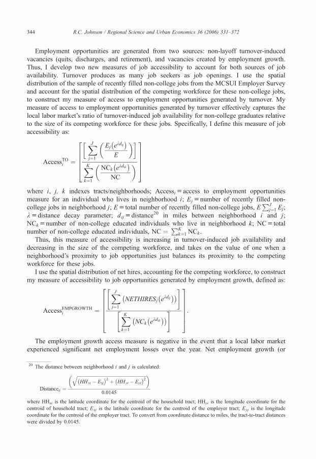
Employment opportunities are generated from two sources: non-layoff turnover-induced
vacancies (quits, discharges, and retirement), and vacancies created by employment growth.
Thus, I develop two new measures of job accessibility to account for both sources of job
availability. Turnover produces as many job seekers as job openings. I use the spatial
distribution of the sample of recently filled non-college jobs from the MCSUI Employer Survey
and account for the spatial distribution of the competing workforce for these non-college jobs,
to construct my measure of access to employment opportunities generated by turnover. My
measure of access to employment opportunities generated by turnover effectively captures the
local labor market’s ratio of turnover-induced job availability for non-college graduates relative
to the size of its competing workforce for these jobs. Specifically, I define this measure of job
accessibility as:
AccessTOi ¼
� XJj¼1
�Ej
�ekdij�
E
�
XKk¼1
�NCk
�ekdik
�NC
�377775
266664
where i, j, k indexes tracts/neighborhoods; Accessiuaccess to employment opportunities
measure for an individual who lives in neighborhood i; Ejunumber of recently filled non-
college jobs in neighborhood j; Eu total number of recently filled non-college jobs, EPJ
j¼1 Ej;
kudistance decay parameter; dijudistance20 in miles between neighborhood i and j;
NCkunumber of non-college educated individuals who live in neighborhood k; NCu total
number of non-college educated individuals, NC ¼PK
k¼1 NCk .
Thus, this measure of accessibility is increasing in turnover-induced job availability and
decreasing in the size of the competing workforce, and takes on the value of one when a
neighborhood’s proximity to job opportunities just balances its proximity to the competing
workforce for these jobs.
I use the spatial distribution of net hires, accounting for the competing workforce, to construct
my measure of accessibility to job opportunities generated by employment growth, defined as:
AccessEMPGROWTHi ¼
XJj¼1
NETHIRESj ekdij
� �� �" #
XKk¼1
NCk ekdik� �� �" #
3777775:
2666664
The employment growth access measure is negative in the event that a local labor market
experienced significant net employment losses over the year. Net employment growth (or
20 The distance between neighborhood i and j is calculated:
Distanceij ¼
� ffiffiffiffiffiffiffiffiffiffiffiffiffiffiffiffiffiffiffiffiffiffiffiffiffiffiffiffiffiffiffiffiffiffiffiffiffiffiffiffiffiffiffiffiffiffiffiffiffiffiffiffiffiffiffiffiffiffiffiffiffiffiHHxi � Exj
� �2 þ HHyi � Eyi
� �2q �0:0145
where HHxi is the latitude coordinate for the centroid of the household tract; HHyi is the longitude coordinate for the
centroid of household tract; Exj is the latitude coordinate for the centroid of the employer tract; Eyj is the longitude
coordinate for the centroid of the employer tract. To convert from coordinate distance to miles, the tract-to-tract distances
were divided by 0.0145.

R.C. Johnson / Regional Science and Urban Economics 36 (2006) 331–372 345
loss) is normalized by the size of the workforce competing for these jobs in the local labor
market.
These two job accessibility measures jointly capture a worker’s proximity to job openings
relative to the competing workers, discounting distant job openings and distant competing
workers by the distance decay parameter k (obtained from the first-stage gravity model
estimation). The estimated distance decay parameter for less-skilled workers was � .101 in
Atlanta, � .149 in Boston, and � .093 in the Los Angles MSA. Thus, using our estimated
distance decay parameter for less-skilled workers in Atlanta, jobs (competing workers) located
at distances of 0, 5, 10, 15, and 20 mi would have weights of 1, .60, .36, .22, and .13,
respectively. Using these measures of job access for the census tracts throughout each of the
MSAs, allows us to also determine the search areas (defined in the MCSUI Household Survey)
within each MSA that are relatively rich in employment opportunities for less-educated
individuals (using the average computed access measures for the census tracts that make up the
various search areas).
5. Descriptive results
I begin by documenting and addressing the extent of spatial mismatch in the Atlanta, Boston,
and Los Angeles MSAs. Is access to employment opportunities for non-college graduates greater
in the suburbs than in the central city? Due to the non-uniform geographic pattern of suburban
job growth, is there significant variation in access within the suburbs? I present descriptive maps
below for Atlanta, but similar spatial patterns of results were found in Boston and Los Angeles,
and are presented in the longer web version of this paper (Johnson, 2004). The focus of the
discussion of results is on black–white differences because these differences are most stark.
However, this study is unique in its access to data from multi-ethnic MSAs, and few previous
studies have examined the SMH as it applies to other ethnic groups. In light of this, Hispanic
differences are also noted where significant.
5.1. Residential segregation
Map 1, entitled bResidential SegregationQ, shows racial residential patterns for the Atlanta
MSA. The minority population of Atlanta contains mostly blacks and relatively few
Hispanics and Asians, while the minority populations are more mixed between the three
groups in Los Angeles and Boston. Blacks are concentrated within a core area of the central
city—almost all neighborhoods are either less than 10% black, or more than 70% black in
each of the MSAs. Blacks are significantly more segregated than Hispanics and Asians. For
example, in Los Angeles and Boston, the black–white dissimilarity index21 was 73 and 70,
respectively. In contrast, the Hispanic–white index was 61 and 55 and the Asian–white index
was 46 and 44 in Los Angeles and Boston, indicating much less segregation (Iceland et al.,
2002). These racial/ethnic differences in the degree of residential segregation have implications
for job search, since we expect the labor market outcomes and job search behavior of racial/
ethnic groups that face greater residential location constraints to be more sensitive to local job
accessibility.
21 The dissimilarity index is the most commonly used measure of housing segregation and represents the percentage of
minority members that would have to change neighborhoods to achieve an even distribution.
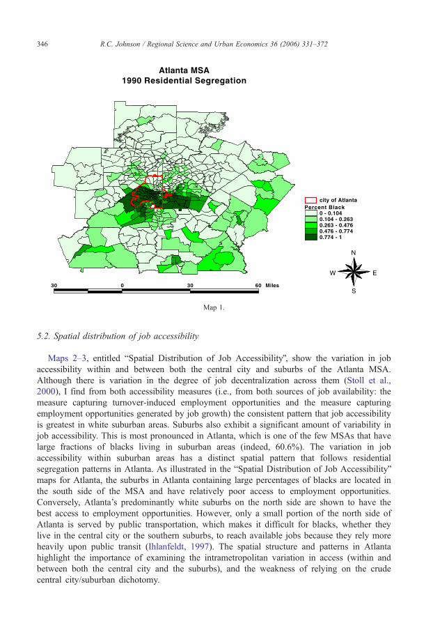
Percent Black0 - 0.1040.104 - 0.2630.263 - 0.4760.476 - 0.7740.774 - 1
city of Atlanta
30 0 30 60 Miles
N
EW
S
Atlanta MSA1990 Residential Segregation
Map 1.
R.C. Johnson / Regional Science and Urban Economics 36 (2006) 331–372346
5.2. Spatial distribution of job accessibility
Maps 2–3, entitled bSpatial Distribution of Job AccessibilityQ, show the variation in job
accessibility within and between both the central city and suburbs of the Atlanta MSA.
Although there is variation in the degree of job decentralization across them (Stoll et al.,
2000), I find from both accessibility measures (i.e., from both sources of job availability: the
measure capturing turnover-induced employment opportunities and the measure capturing
employment opportunities generated by job growth) the consistent pattern that job accessibility
is greatest in white suburban areas. Suburbs also exhibit a significant amount of variability in
job accessibility. This is most pronounced in Atlanta, which is one of the few MSAs that have
large fractions of blacks living in suburban areas (indeed, 60.6%). The variation in job
accessibility within suburban areas has a distinct spatial pattern that follows residential
segregation patterns in Atlanta. As illustrated in the bSpatial Distribution of Job AccessibilityQmaps for Atlanta, the suburbs in Atlanta containing large percentages of blacks are located in
the south side of the MSA and have relatively poor access to employment opportunities.
Conversely, Atlanta’s predominantly white suburbs on the north side are shown to have the
best access to employment opportunities. However, only a small portion of the north side of
Atlanta is served by public transportation, which makes it difficult for blacks, whether they
live in the central city or the southern suburbs, to reach available jobs because they rely more
heavily upon public transit (Ihlanfeldt, 1997). The spatial structure and patterns in Atlanta
highlight the importance of examining the intrametropolitan variation in access (within and
between both the central city and the suburbs), and the weakness of relying on the crude
central city/suburban dichotomy.
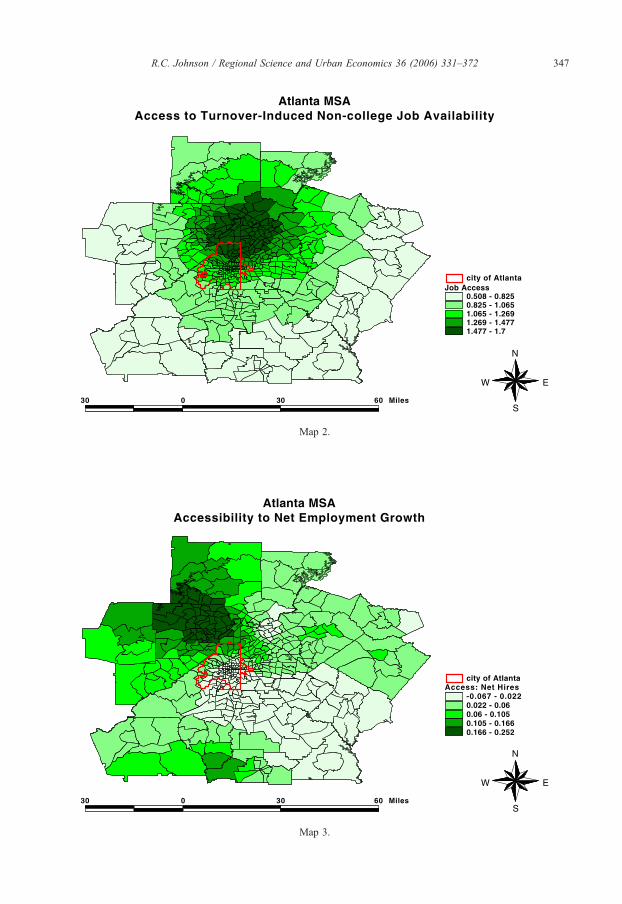
Access: Net Hires -0.067 - 0.0220.022 - 0.060.06 - 0.1050.105 - 0.1660.166 - 0.252
city of Atlanta
30 0 30 60 Miles
N
EW
S
Atlanta MSAAccessibility to Net Employment Growth
Map 3.
Job Access 0.508 - 0.8250.825 - 1.0651.065 - 1.2691.269 - 1.4771.477 - 1.7
city of Atlanta
30 0 30 60 Miles
N
EW
S
Atlanta MSAAccess to Turnover-Induced Non-college Job Availability
Map 2.
R.C. Johnson / Regional Science and Urban Economics 36 (2006) 331–372 347
Tot
al N
et H
ires,
pas
t yea
r
Miles from Average Worker's Home
Blacks Whites
0 5 10 15 20
-5,000
0
5,000
10,000
15,000
20,000
25,000
30,000
35,000
40,000
Fig. 1. Net hires by distance from worker’s home Atlanta, 1992–1993.
R.C. Johnson / Regional Science and Urban Economics 36 (2006) 331–372348
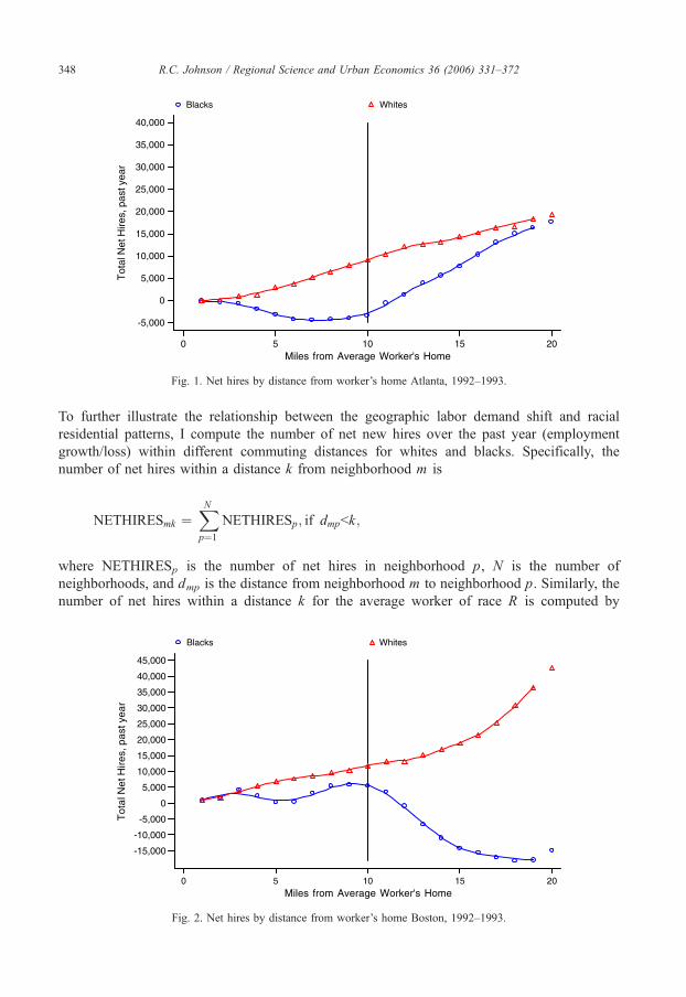
To further illustrate the relationship between the geographic labor demand shift and racial
residential patterns, I compute the number of net new hires over the past year (employment
growth/loss) within different commuting distances for whites and blacks. Specifically, the
number of net hires within a distance k from neighborhood m is
NETHIRESmk ¼XNp¼1
NETHIRESp; if dmpbk;
where NETHIRESp is the number of net hires in neighborhood p, N is the number of
neighborhoods, and dmp is the distance from neighborhood m to neighborhood p. Similarly, the
number of net hires within a distance k for the average worker of race R is computed by
Tot
al N
et H
ires
, pas
t yea
r
Miles from Average Worker's Home
Blacks Whites
0 5 10 15 20
-15,000
-10,000
-5,000
0
5,000
10,000
15,000
20,000
25,000
30,000
35,000
40,000
45,000
Fig. 2. Net hires by distance from worker’s home Boston, 1992–1993.

Tot
al N
et H
ires
, pas
t yea
r
Miles from Average Worker's Home
Blacks Whites
0 5 10
-70,000
-60,000
-40,000
-20,000
-15,000
-10,000
-5,000
0
Fig. 3. Net hires by distance from worker’s home Los Angeles, 1992–1993.
R.C. Johnson / Regional Science and Urban Economics 36 (2006) 331–372 349
summing across neighborhoods, weighting by the fraction of the racial group’s population that
resides in each neighborhood:
NETHIRESRk ¼1XN
m¼1popRm
1CCCCAXNm¼1
XNp¼1
popRm4 NETHIRESp� �
; if dmpbk;
0BBBB@
where popRm is the population of group R in neighborhood m. These results are shown in Figs. 1
2 and 3. The vertical line at 10 mi marks the average one-way commute distance for non-college
graduates. Figs. 1 2 and 3 reveal that the degree of employment growth (loss) over the past year
(1993) within different commuting distances of the average black worker were significantly less
(more) than that experienced for the average white worker, in the three MSAs. For example, in
Atlanta (Fig. 1), about 5000 jobs were lost within a 10-mi radius of the average black worker,
while about 5000 jobs were gained within that radius for the average white worker. Similar
patterns are found in Boston and Los Angeles.22 Furthermore, the distribution of accessibility to
employment growth experienced by black workers is more tightly distributed around the lower
mean (at various commuting distances), due to racial segregation. Similar patterns are observed
22 The differences in magnitude (in absolute value) in the overall levels of annual employment growth between the
MSAs are in part driven by the size of the respective MSAs (total employment (1993) 1,456,178 in Atlanta; 2,282,136 in
Boston; 3,495,246 in Los Angles from County Business Pattern data). As well, Los Angeles may have been suffering
through a post 1980s slump, as well as from likely negative labor market effects of the racial disturbances of April 1992
and the Northridge earthquake in 1994 (Holzer, 1996). In contrast, Atlanta was enjoying a pre-1996 Olympics boom
during this period. Recall the surveys were administered to firms in the period between 1992 and 1994, during which
time the national economy was recovering from recession.

R.C. Johnson / Regional Science and Urban Economics 36 (2006) 331–372350
for Hispanic–white differences in average accessibility to job growth in Los Angeles and
Boston, though these differences are smaller in magnitude relative to the black–white differences
(results available from author upon request).
I use the job accessibility measures to determine which search areas are rich in
employment opportunities for non-college graduates. Search areas are rich in non-college
jobs if the number of jobs relative to the supply of non-college educated individuals is high
(using the average computed access measures for the census tracts that make up the various
search areas). The northern suburbs of Atlanta (Marietta/Smyrna, Roswell/Alpharetta,
Norcross), the Metro West area of Boston, and the West San Fernando Valley area of Los
Angeles, are classified as job rich. These job-rich search areas are consistent with other
sources (see, for example, Stoll et al. (2000), and Ihlanfeldt (1997) for Atlanta). All of these
job-rich search areas are located in predominantly white suburbs more than 10 mi from the
centroid of black residential concentration, and these areas are not served by public
transportation. I find that 75% of individuals who self-reported not searching in these job-rich
areas, did not do so because of reasons related to travel distance, lack of transportation, and
traffic problems.
These patterns are consistent with spatial mismatch-spatial asymmetries in non-college job
availability and the residential concentration of minorities. I next discuss the empirical model I
use to investigate the effects of access to employment opportunities and dimensions of job search
behavior on search duration.
6. Econometric model
Using a sample of individuals who had recently conducted a job search,23 search duration
is analyzed by estimating the conditional probability (hazard) of a search spell ending in a
particular week via obtaining a new job. Even among spells that are not right-censored, not all
search spells end in employment—some individuals stop searching without accepting a new job
offer. I am able to determine whether individuals have successfully completed their job search
(i.e., the individual found a job and is no longer searching) through job search survey questions
about when last searched, duration of search, whether individuals received a job offer while
searching, and current job tenure.24 Individuals who continued their search after obtaining a job
are assumed to have taken a temporary/transitional job.
This job search analysis is one of the few that includes both individuals searching while
employed (on-the-job search) and those searching while unemployed. I distinguish between
individuals who obtain transitional employment while continuing to search, and those who
successfully complete a job search. Analyzing job search spells, rather than unemployment
spells, is an important distinction. I find that a sizeable fraction of less-educated searchers took
transition jobs while continuing to search, to alleviate part of the financial burden that
accompanies unemployment.
24 Specifically, individuals are classified as having successfully completed their job search if the following 5 conditions hold:
(1) must have searched within the last year and must have contacted an employer within the last month of search; (2) must have
received a job offer while searching; (3) must have obtained a current job within the last year; (4) cannot be involuntarily
working part-time due to demand-side constraints, and (5) must have stopped searching after obtaining current job.
23 The sample contains individuals who had begun a job search within the last 12 months of the survey interview date.
Individuals who began their job search more than a year before the interview date are not included in the analysis (i.e.,
spells already in progress as of a year prior to the survey interview date (left-censored spells) are dropped).

R.C. Johnson / Regional Science and Urban Economics 36 (2006) 331–372 351
The hazard is specified in a logit form, where the explanatory variables include a constant, the
direct duration effect on the hazard (i.e., the influence of spell duration holding all other variables
constant), and a vector of characteristics (X): k(T; X)=1 / (1�exp[bX +a1T +a2T2]).25
I model the dependence of the hazard rate on time in the spell by the duration of the
current spell and its square.26 The regression analysis focuses on the effects of job accessibility,
and whether these effects differ by race/ethnicity and education in the ways predicted by the
spatial job search model. The other search-related explanatory variables that make up the vector
X include: the number of hours spent searching per week, the number of hours searched squared,
the relative reservation wage, the number of employed persons in the individual’s social network
(proxy for the quality of the individual’s social network), the reservation commute time (in
minutes), dummy variables indicating whether individual had access to a car while searching,
whether individual lives in (low) medium or high poverty-rate neighborhood, whether individual
searched in a job-rich search area (interacted with non-college graduate dummy), whether
individual used formal search methods, whether individual searched with credential-based
references, and whether searched with network-based references.
I attempt to separate the effects of the neighborhood location(spatial isolation) from the
characteristics of the neighborhoods themselves (social isolation). I include neighborhood
poverty measures to capture the effects of the latter.
Since job accessibility may affect search duration directly as well as indirectly through its
effects on job search behavior, the model is estimated with and without the search method
variables. The rationale for inclusion of the search method variables is that search behavior may
have independent effects on search duration that are of interest. As well, inclusion of the full set of
search method variables minimizes concerns that the estimated effects of job accessibility are
driven by unobserved heterogeneity.
The rationale for exclusion of the search method variables is that some of them may be
considered endogenous and, hence, a source of bias. A potential endogeneity issue with respect
to search methods arises due to the fact that search methods—both how (e.g., open market
search, use of formal labor market intermediaries, social network search) and where—are self-
selected by the searcher, and thus are a function of the expected cost-effectiveness of each for
that person (Holzer, 1988). This could upward-bias the estimates of the effects of search methods
(e.g., the effect of searching in a job-rich area). As well, some searchers may have more prior
information about the wage rates paid and the probability of obtaining an offer at specific firms
and, as a result, may have a higher return from search activity by adopting systematic search
without having to resort to using newspaper ads, job advertisements, or labor market
intermediaries. This will produce a downward bias of the effect of these search method
variables included in the model.
25 For spells that are completed during the sampling period the density function equals the probability of a search spell
ending via finding a new job in week t times the conditional probability of the individual’s search spell not ending in each of
the prior t�1 weeks. This is specified as fi t0i; tð Þ ¼ ki t0i; tð Þjt�1r¼1 1� ki toi; rð Þ½ �. For incomplete spells, the survivor
function equals the probability that the individual’s search spell did not end via finding a new job in each of the prior tiweeks. The survivor function is specified as 1� Fi t0i; tð Þ½ � ¼jti
r¼1 1� ki t0i; rð Þ½ �. Complete spells (iaC) are combined
with incomplete spells (ia IC) to form the likelihood function which equals L ¼jiaC fi t0i; tð ÞjiaIC 1� Fi t0i; tð Þ½ �. Thelikelihood function is maximized with respect to the explanatory variables to obtain coefficient estimates.26 I experimented with a variety of other specifications to model duration dependence within this discrete time
framework, including the log of current duration and its square. I also experimented with a number of continuous time
models using different distributional assumptions for the duration data. The results across these different specifications
were not fundamentally different and did not change the basic results reported below.

R.C. Johnson / Regional Science and Urban Economics 36 (2006) 331–372352
The job search literature suggests that some of the choice variables of a searcher vary over the
course of the search spell. In this paper, however, I must assume fixed choices for the variables in
the job search model because the information collected—in particular, the reservation wage and
the number of hours spent searching per week—refers to the level of these variables that prevailed
in the last (most recent) month of the search spell rather than at the beginning of the search spell.
The resulting bias of not allowing time-variation or intensity variation in search strategies over the
course of the spell could upward bias estimated effects of search intensity and could bias toward
zero the estimated effect of reservation wages, if the stationarity assumption does not hold. Such
biases may be reinforced by the presence of unobserved skills, which should be correlated with
reservation wages, search intensity, and the probability of job search success in a given week.
Thus, I estimate models with and without the search method variables. The inclusion of duration
variables and the extensive set of controls in the full model minimize concerns that the estimated
effects of job accessibility are driven by unobserved heterogeneity.
To minimize concerns about endogenous migration, I fix job accessibility as of the beginning
of the spell (i.e., I use job accessibility measures based on the respondent’s residence when the
search began).27 This addresses a specific kind of endogeneity ex-post—namely, that people
might move to jobs. I also experiment with a variety of interactions of job accessibility with
factors that affect the amount of spatial frictions searchers face (such as car ownership and
measures of the quality of social networks). These interactions are used to test the hypothesis
that those facing greater search frictions are more sensitive to local labor market demand.
The effects of job accessibility on college-educated labor are estimated as a robustness check,
since we do not expect to find significant effects of job accessibility for college-educated workers. To
minimize the loss of occupation-specific skills acquired, more-skilled workers will restrict the range
of jobs they seek to those in which their skills are most valued. As a result, more-skilled workers (job
vacancies) will expect a lower density of suitable matches and (workers/employers) will pursue more
spatially extensive search (less responsive to local opportunities) and rely on formal information
networks more heavily, in order to locate distant jobs (applicants) (Simpson, 1992).
7. Empirical results
7.1. Summary statistics
In Table 1, I present the summary statistics for minority/white non-college graduates
separately by job accessibility, to explore the relationship between search intensity and local
job accessibility. The prevalence of job search activity for minority (blacks, Hispanics,
Asians) non-college graduates is significantly lower among those with poor accessibility to
employment growth—48.4% of those with high accessibility to net employment growth had
searched for work within the past year, relative to only 29.2% of those with low accessibility
to net employment growth. As well, current employment is more often the result of the
success of a recent job search among individuals with high accessibility to job growth
(13.0% versus 3.8%), relative to those with low accessibility. Among the currently employed,
significantly higher fractions of minority non-college graduates with high accessibility to net
employment growth had recently begun a job search while on the current job, and higher
fractions had searched within the past year more generally, relative to minority non-college
27 Only about 5% of the sample changed residential locations while the job search was still ongoing; not enough time
had elapsed to assess what percent changed residential locations after a successful job search.

Table 1
Employment and the prevalence of job search activity among non-college graduates by accessibility to employmen
growtha,b
Minorities Whites
Low access to
job growth
High access to
job growth
Low access
to job growth
High access
to job growth
Searched within past year .2920 .4837 .2813 .2720
Currently employed .7868 .7706 .8806 .8801
Current employment result of:
Success of most recent job search (within past year) .0384 .1295 .0882 .0619
Accepted transitional job offer, still searching .0212 .0293 .0159 .0497
Began search while on current job, still searching .0545 .1540 .0482 .0182
Began search while on current job, stop search
w/o accept offer
.0885 .0683 .0557 .0539
Have not recently searched (within past year) .7974 .6189 .7919 .8163
Current nonemployment result of:
Not searching (OLF—have not searched
within past year)
.3780 .1714 .1782 .0796
Still searching .4426 .7517 .6408 .8362
Searched within past year, but stopped search
w/o accept offer
.1690 .0609 .1810 .0823
a Here I define low accessibility to net employment growth as accessibility that is less than or equal to� .03; I define highaccessibility to net employment growth as accessibility that is greater than or equal to +.03. The (sample-weighted
proportion of minority non-college graduates with low accessibility was 52.1% (N =2054), and the proportion with high
accessibility was only 9.6% (N =384). In contrast, the (sample-weighted) proportion of white non-college graduates with
low accessibility was 33.9% (N =406), and the proportion with high accessibility was 37% (N =445). I experimented with
alternative thresholds for low/high job accessibility, none of which qualitatively changed the patterns shown in these tablesb Sample includes all MCSUI household survey respondents in the Atlanta, Boston, and Los Angeles MSAs, excep
college graduates, and those who reported being sick/maternity, retired, permanently disabled, homemakers, or students
R.C. Johnson / Regional Science and Urban Economics 36 (2006) 331–372 353
t
)
.
t
.
graduates with low accessibility. These results appear to reflect the greater stability of
existing job matches in low employment growth areas, thus reducing turnover-induced job
availability. bDiscouragedQ workers are more prevalent among minority non-college graduates
with poor accessibility, as I find they have higher fractions reporting ending job searches
without accepting a new job offer amongst both the employed and non-employed
populations, relative to minority non-college graduates with high accessibility.
In contrast, columns (3) and (4) of Table 1 do not show these same patterns by accessibility to
net employment growth among white non-college graduates. The search activity of white non-
college graduates appears to be less sensitive to accessibility to net employment growth.
Whether these correlations simply reflect worker heterogeneity across residential locations is
unclear without a more complete multivariate analysis.
For the remainder of the analysis, I restrict my sample to individuals who began a job search
within the past year, and I focus my regression analysis on the effects of spatial structure on the
job search behavior and job search outcomes of labor force participants. In Table 2, I present the
means of the variables of the duration (hazard) model separately by race/ethnicity. As shown in
Table 2, 21% of the sample had successfully completed their job search by obtaining new jobs
(as of the survey interview date). As of the survey interview date, 7.9% were working in
transitional jobs while continuing the job search; 17.7% had begun searching while on the job
and were still searching; 22.9% had begun searching while on the job and had stopped searching
without obtaining new jobs; 25.6% were not employed and were still searching; 4.8% were not
employed and had stopped searching.

Table 2
Job search sample meansa (standard errors) by race/ethnicity
All [full sample] White Black Hispanic
Search duration (weeks)b 10.8 (.8439) 11.7 (1.3613) 11.2 (1.6367) 9.9 (1.2511)
Destination frequencies
Successfully completed job search .2099 .2787 .1350 .0982
Accepted transitional job offer, still searching .0788 .0528 .1077 .1201
Began search while on-the-job, still searching .1770 .1509 .1990 .1788
Began search while on-the-job,
stop search w/o accept offer
.2290 .2305 .2303 .2335
Not employed, still searching .2563 .2537 .2639 .2915
Not employed, stopped search
w/o accepting offer
.0478 .0314 .0640 .0780
Search method variables
Number of search methods used 2.4 (.0522) 2.4 (.0827) 2.6 (.0882) 2.2 (.0821)
Open market search .9278 .9530 .9593 .8595
Social network search .8191 .8014 .8636 .8204
Number employed in social network (max: 3) 1.6 (.0728) 1.9 (.1032) 1.6 (.1289) 1.2 (.1126)
Use state/temporary employment agency .3047 .2987 .4875 .2642
Union/school/private employment service .3274 .3818 .3043 .2207
Credential-based references .7875 .8865 .7776 .6048
Network-based references .5732 .6398 .6325 .4361
Number of hours spent searching per week 8.7 (.7444) 8.7 (1.2491) 8.6 (.9296) 9.2 (.9610)
Relative reservation wage 1.03 (.0298) 1.077 (.0500) 1.049 (.0580) .968 (.0276)
Spatial search variables
Access to car when searched .8304 .9087 .7489 .7151
Reservation commute time (minutes) 45.1 (1.3243) 43.8 (1.9367) 50.5 (2.1157) 44.2 (1.9366)
Among non-college grads:
Access to turnover-induced job availability 1.059 (.0160) 1.0465 (.0329) 1.1170 (.0260) 1.0382 (.0098)
Access to employment growth .0560 (.0368) .0885 (.0516) � .0070 (.0082) � .0309 (.0038)
Searched in job-rich area .3290 .4481 .2758 .1927
Live in b10% poverty tract .6429 .8879 .4381 .2898
Live in 10–30% poverty tract .2826 .1081 .4356 .5195
Live in N30% poverty tract .0745 .0040 .1263 .1908
Metropolitan area
Atlanta .1478 .1857 .3099 .0125
Boston .2674 .3918 .1463 .0424
Los Angeles .5909 .4457 .5171 .9093
Demographic variables
Age (years) 34.5 (.6764) 36.3 (1.1488) 31.3 (.7710) 32.8 (.8761)
Female .4803 .4891 .5835 .4117
Married .5507 .5857 .3855 .5350
Child care concerns .1538 .1430 .1810 .1685
Received unemployment insurance .2095 .2319 .1557 .2297
Received AFDC .0837 .0389 .2435 .1067
Work-limiting health condition .1126 .1144 .1285 .1151
Human capital variables
Dropout .1734 .0619 .0804 .4545
HS grad/GED .2356 .2457 .2779 .2199
R.C. Johnson / Regional Science and Urban Economics 36 (2006) 331–372354
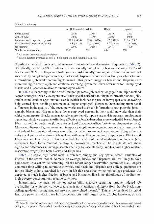
28 Computed standard errors on weighted means are generally not correct, since population rather than sample sizes is used
during the computation. But standard errors for unweighted means give a fairly good indication of the relevant standard errors
Table 2 (continued)
All [full sample] White Black Hispanic
Some college .2842 .2734 .4385 .2273
College grad .3037 .4150 .2009 .0960
Full-time work experience (years) 11.7 (.6458) 12.8 (1.0754) 9.3 (.8169) 11.3 (.8930)
Part-time work experience (years) 1.8 (.2613) 1.8 (.4041) 1.0 (.1455) 2.5 (.5001)
Job training .2600 .3216 .2479 .1800
Number of observations 1205 313 409 368
a All means here are sample-weighted.b Search duration averages consist of both complete and incomplete spells.
R.C. Johnson / Regional Science and Urban Economics 36 (2006) 331–372 355
Significant racial differences exist in search outcomes (see destination frequencies, Table 2).
Specifically, while 27.9% of whites had successfully completed job searches, only 13.5% of
blacks and 9.8% of Hispanics had done so. Additionally, among individuals who had not
successfully completed job searches, blacks and Hispanics were twice as likely as whites to take
a transitional job while continuing to search. This pattern suggests blacks and Hispanics are
more willing to accept a job and continue searching, given the lower offer rates for unemployed
blacks and Hispanics relative to unemployed whites.
In Table 2, according to the search method patterns, job seekers engage in multiple-method
search strategies. Nearly everyone used their social networks to obtain information about jobs,
and/or conducted an open market search (which includes the use of newspaper ads, answering
help-wanted signs, sending a resume or calling an employer). However, there are important racial
differences in the quality of the social networks used to obtain information about potential jobs—
namely, blacks and Hispanics have fewer employed persons in their social networks than their
white counterparts. Blacks appear to rely more heavily upon state and temporary employment
agencies, which we expect to offer less effective referrals than other more credential-based formal
labor market intermediaries (labor union/school placement officer/private employment service).
Moreover, the use of government and temporary employment agencies are in many cases search
methods of last resort, and employers often perceive government agencies as listing primarily
entry-level jobs and referring job seekers with very little screening of applicants. Blacks and
Hispanics are less likely to have searched for work with credential-based references (i.e.,
references from former/current employers, co-workers, teachers). The results do not show
significant differences in average search intensity by race/ethnicity. Whites have higher relative
reservation wages than both blacks and Hispanics.
Table 2 displays significant racial differences among the key spatial search variables of
interest in the search model. Namely, on average, blacks and Hispanics are less likely to have
had access to a car while searching, blacks report longer reservation commutes (i.e., longest
commute time willing to commute to work), and black and Hispanic non-college graduates are
far less likely to have searched for work in job-rich areas than white non-college graduates. As
expected, a much higher fraction of blacks and Hispanics live in neighborhoods of medium-to-
high poverty concentrations relative to whites.
Interestingly, the mean of the job accessibility measure capturing turnover-induced job
availability for white non-college graduates is not statistically different from that for black non-
college graduates (using standard errors of unweighted means).28 This is the result of historical
land use patterns, which have left the central city with large stocks of jobs. However, as was
.
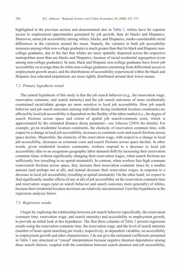
R.C. Johnson / Regional Science and Urban Economics 36 (2006) 331–372356
highlighted in the previous section and demonstrated also in Table 1, whites have far superior
access to employment opportunities generated by job growth, than do blacks and Hispanics.
Moreover, mean job accessibility among whites, blacks, and Hispanics, masks considerable racial
differences in the variation around the mean. Namely, the variance in both job accessibility
measures amongwhite non-college graduates is much greater than that for black andHispanic non-
college graduates, due to the fact that whites are more spatially dispersed across the respective
metropolitan areas than are blacks and Hispanics, because of racial residential segregation (even
among non-college graduates). In sum, black and Hispanic non-college graduates have lower job
accessibility on average than do white non-college graduates (stemming from differential access to
employment growth areas), and the distributions of accessibility experienced within the black and
Hispanic less-educated populations are more tightly distributed around their lower means.
7.2. Primary hypothesis tested
The central hypothesis of this study is that the job search behavior (e.g., the reservation wage,
reservation commute, and search intensity) and the job search outcomes of more residentially
constrained racial/ethnic groups are more sensitive to local job accessibility. How job search
behavior and job search outcomes (among individuals facing residential location constraints) are
affected by local job accessibility is dependent on the fluidity of the labor market (i.e., the degree of
search frictions across space and extent of spatial job search/commute costs, which is
approximated by the estimated distance decay parameter—see Johnson (2004) for details). For
example, given residential location constraints, the elasticity of reservation commute time, with
respect to a change in local job accessibility, increases as commute costs and search frictions across
space decline. Meanwhile, the elasticity of the reservation wage, with respect to a change in local
job accessibility, decreases as commute costs and search frictions across space decline. In other
words, given residential location constraints, workers respond to a decrease in local job
accessibility (due to an exogenous geographic labor demand shift) by increasing their reservation
commute times without significantly changing their reservation wages, when search frictions are
sufficiently low (resulting in no spatial mismatch). In contrast, when workers face high commute
costs/search frictions across space, they increase their reservation commute times by a smaller
amount (and perhaps not at all), and instead decrease their reservation wages, in response to a
decrease in local job accessibility (resulting in spatial mismatch). On the other hand, we expect to
find significantly smaller effects (if any at all) of job accessibility on the reservation commute time
and reservation wages (and on search behavior and search outcomes more generally) of whites,
because their residential location decisions are relatively unconstrained. I test this hypothesis in the
regression analyses below.
7.3. Regression results
I begin by exploring the relationship between job search behavior (specifically, the reservation
commute time, reservation wage, and search intensity) and accessibility to employment growth,
to provide an initial look at this hypothesis. The first three columns of Table 3 present regression
results using the reservation commute time, the reservation wage, and the level of search intensity
(number of hours spent searching per week), respectively, as dependent variables, on accessibility
to employment growth and other characteristics. I do not give the estimated coefficients presented
in Table 3 any structural or bcausalQ interpretation because negative duration dependence among
these search choices, coupled with the correlation between search duration and job accessibility,
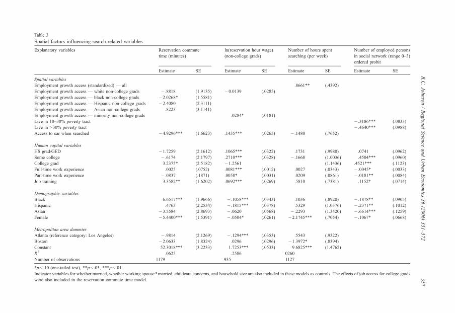
Table 3
Spatial factors influencing search-related variables
Explanatory variables Reservation commute
time (minutes)
ln(reservation hour wage)
(non-college grads)
Number of hours spent
searching (per week)
Number of employed persons
in social network (range 0–3)
ordered probit
Estimate SE Estimate SE Estimate SE Estimate SE
Spatial variables
Employment growth access (standardized) — all .8661** (.4392)
Employment growth access — white non-college grads � .8818 (1.9135) �0.0139 (.0285)
Employment growth access — black non-college grads �2.0268* (1.5581)
Employment growth access — Hispanic non-college grads �2.4080 (2.3111)
Employment growth access — Asian non-college grads .8223 (3.1141)
Employment growth access — minority non-college grads .0284* (.0181)
Live in 10–30% poverty tract � .3186*** (.0833)
Live in N30% poverty tract � .4640*** (.0988)
Access to car when searched �4.9296*** (1.6623) .1435*** (.0265) � .1480 (.7652)
Human capital variables
HS grad/GED �1.7259 (2.1612) .1065*** (.0322) .1731 (.9980) .0741 (.0962)
Some college � .6174 (2.1797) .2710*** (.0328) � .1668 (1.0036) .4504*** (.0960)
College grad 3.2375* (2.5182) �1.2561 (1.1436) .4521*** (.1123)
Full-time work experience .0025 (.0752) .0081*** (.0012) .0027 (.0343) � .0045* (.0033)
Part-time work experience � .0837 (.1871) .0058* (.0031) .0209 (.0861) � .0181** (.0084)
Job training 3.3582** (1.6202) .0692*** (.0269) .5810 (.7381) .1152* (.0714)
Demographic variables
Black 6.6517*** (1.9666) � .1058*** (.0343) .1036 (.8920) � .1878** (.0905)
Hispanic .4763 (2.2534) � .1815*** (.0378) .5329 (1.0376) � .2371** (.1012)
Asian �3.5584 (2.8693) � .0620 (.0568) � .2293 (1.3420) � .6614*** (.1259)
Female �5.4400*** (1.5391) � .0504* (.0261) �2.1745*** (.7054) � .1067* (.0668)
Metropolitan area dummies
Atlanta (reference category: Los Angeles) � .9814 (2.1269) � .1294*** (.0353) .5543 (.9322)
Boston �2.0633 (1.8324) .0296 (.0296) �1.3972* (.8394)
Constant 52.3018*** (3.2233) 1.7253*** (.0533) 9.6825*** (1.4762)
R2 .0625 .2586 0260
Number of observations 1179 935 1127
*p b .10 (one-tailed test), **p b .05, ***p b .01.
Indicator variables for whether married, whether working spouse*married, childcare concerns, and household size are also included in these models as controls. The effects of job access for college grads
were also included in the reservation commute time model.
R.C.Johnson/RegionalScien
ceandUrbanEconomics
36(2006)331–372
357

R.C. Johnson / Regional Science and Urban Economics 36 (2006) 331–372358
may bias estimated effects of job accessibility. Instead, I use this framework to summarize some
of the relationships between these aspects of job search behavior and job accessibility. The results
suggest how search methods chosen by job seekers may be shaped by the interaction of two
important features of urban spatial structure: (1) extent of involuntary residential segregation, and
(2) the job searcher’s proximity to employment opportunities.
As shown in the first column of Table 3, I find racial differences in the association of job
accessibility and reservation commute time.29 While the magnitudes of the associations are not
particularly large, the patterns are nonetheless interesting. Black non-college graduates with poor
accessibility to employment growth report longer reservation commute times than comparable
blacks with high accessibility to employment growth, while white non-college graduates’
reservation commute times are less sensitive to accessibility to employment growth. This
suggestive evidence of blacks’ greater willingness to adjust their commute patterns in response
to a geographic labor demand shift is consistent with the predictions of theory, given the greater
residential mobility constraints facing blacks. As well, blacks report longer reservation commute
times on average for any given level of job accessibility. I also find that individuals who lacked
access to a car report longer reservation commute times, likely due to their reliance on slower forms
of transportation. As expected, college graduates and workers with job training report longer
reservation commute times, reflecting more geographically expansive commute patterns among
highly educated workers (which parallels the smaller distance decay parameters estimated for
higher-income workers—see Johnson (2004)).
I restrict my sample to non-college graduates to examine the relationship between reservation
wages and job accessibility. These regression results are reported in the second column of Table 3. I
find racial differences in the associations of job accessibility and reservation wages as well. Again,
while the magnitudes of the associations are not particularly large, the patterns are nonetheless
interesting. Minority non-college graduates with poor accessibility to employment growth have
lower reservation wages than comparable minorities with high accessibility to employment growth,
while white non-college graduates’ reservation wages are insensitive to accessibility to employment
growth. These results are consistent with the subsequent emergence of spatial mismatch (i.e.,
otherwise identical individuals achieve different labor market outcomes because of their residential
location) among minorities and not among whites, as predicted and discussed in the theoretical
section. Blacks and Hispanics have lower reservation wages for any given level of job accessibility.
I also find that individuals who did not have access to a car have lower reservation wages.
This association could be picking up fixed unobserved worker quality, as previous employment
success may have enabled individuals to buy a car. The estimated associations of the set of
standard human capital variables included in the model are all significant and in the expected
directions. Of course, unobserved skills correlated with residential location, likely account for
some of the estimated associations of job accessibility and reservation wages in this simple
model; but the existence of racial differences in the correlations of job accessibility and
reservation wages is clear from this analysis.
I report the results for search intensity in the third column of Table 3. I find that individuals
with better access to employment growth search more intensely (i.e., they spend more hours
per week searching). This may reflect greater expected returns to search for individuals
residing in areas with better local labor market demand conditions, or it may reflect their lower
29 I standardize both job accessibility measures to have mean 0, standard deviation 1 (using the respective mean job
accessibility (and standard deviation) across all neighborhoods of the MSAs) in the regression, so that a one-unit change
in the standardized job access measure can be interpreted as a one standard deviation change.

R.C. Johnson / Regional Science and Urban Economics 36 (2006) 331–372 359
search costs due to being able to identify alternative vacancies easier. The magnitude of the
associations of job accessibility and search intensity did not differ significantly by race (not
shown). I do not find significant differences in search intensity between the different racial/
ethnic groups.
In the fourth column of Table 3, I also present evidence suggestive of the relationship
between the quality of an individual’s social networks in connecting him/her to potential job
opportunities (proxied by the number of employed persons in an individual’s social network)
and the concentration of neighborhood poverty. The results suggest that individuals who live
in medium and high poverty neighborhoods have poorer quality social networks, consistent
with the social isolation hypothesis (Wilson, 1987, 1996). Whether these results capture a
truly causal relation, and thus one of the negative externalities of concentrated poverty, is
unclear from this simple model, but I note the significant correlations. As well, minorities
still have poorer quality social networks after controlling for these other factors.
7.4. Hazard model results
Table 4 contains the reduced-form hazard estimates of the effects of the extensive set of
explanatory variables in my job search model on the conditional probability of a search spell
ending via obtaining a new job in a given week. The average percentage changes in the hazard
due to simulated changes in the explanatory variables are displayed in Table 4.30 The effects of
the spatial search-related variables reveal the importance of spatial aspects of the labor market in
shaping the structure of opportunity.
The most insightful result of the analysis is the differential effect of access by race (and
education). Importantly, I find that the patterns of racial differences in the effects of job
accessibility mirror the patterns of racial differences in the extent of residential location
constraints (documented in the residential segregation literature), as predicted by theory.
Specifically, using the full hazard model specification, I find that increasing accessibility to
turnover-induced job availability from its mean value to one standard deviation above its
mean, increases the hazard (of ending the search via finding a new job) by 86.7% for
black non-college graduates and by 65.1% for Hispanic non-college graduates, while small
statistically insignificant effects are found for whites and Asian non-college graduates. I
find that increasing accessibility to job opportunities generated by employment growth from
its mean value to one standard deviation above its mean, increases the hazard by 29.6%
for black non-college graduates and increases the hazard by 64.6% for Hispanic non-
college graduates, while having small and insignificant effects for white and Asian non-
college graduates. In sum, the length of job search duration is extremely sensitive to
changes in access to employment opportunities for less-educated blacks and Hispanics,
while the length of job search duration for similarly educated whites and Asians is
insensitive to proximity to employment opportunities. These results are robust to the
30 Due to the nonlinearity of the model, average effects of discrete changes in explanatory variables are calculated
throughout this paper by evaluating the effect of varying the explanatory variable of interest in a given way for each
individual (holding all other variables constant and evaluated at the beginning of the spell), and then computing the sample
weighted mean of these effects (e.g., the percentage change in the hazard, or the change in the probability that a search ends
spell within six months). Sample weights are not used to estimate the coefficients of the hazard model to avoid introducing
additional heteroscedasticity, and because factors affecting the weights are controlled for in themodel. I do, however, use the
sample weights to weight the observations when computing the average (marginal) effects and computing the
decomposition estimates, so that these results are representative of a sample of recent job searchers in these MSAs.
-
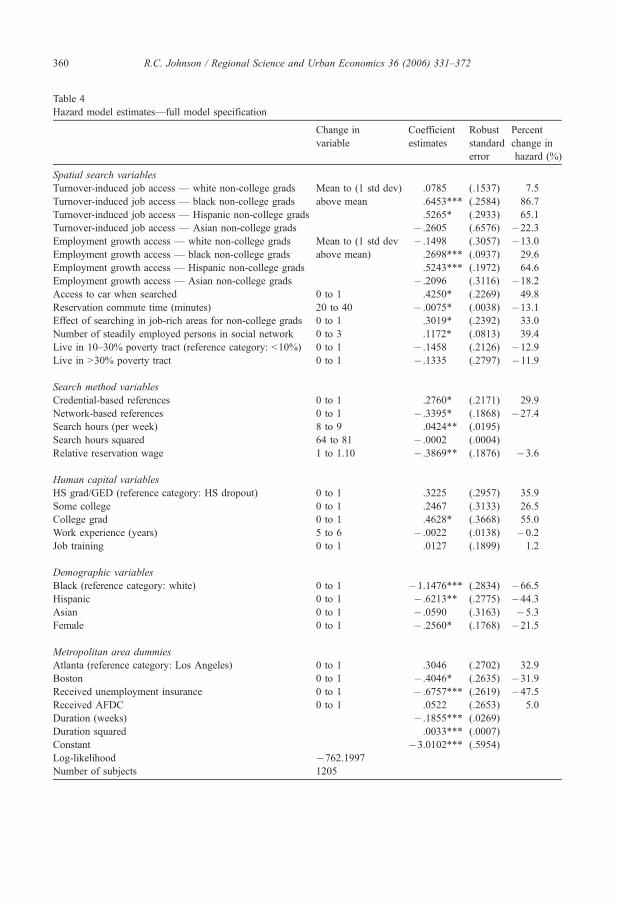
Table 4
Hazard model estimates—full model specification
Change in
variable
Coefficient
estimates
Robust
standard
error
Percent
change in
hazard (%)
Spatial search variables
Turnover-induced job access — white non-college grads Mean to (1 std dev)
above mean
.0785 (.1537) 7.5
Turnover-induced job access — black non-college grads .6453*** (.2584) 86.7
Turnover-induced job access — Hispanic non-college grads .5265* (.2933) 65.1
Turnover-induced job access — Asian non-college grads � .2605 (.6576) �22.3Employment growth access — white non-college grads Mean to (1 std dev
above mean)
� .1498 (.3057) �13.0Employment growth access — black non-college grads .2698*** (.0937) 29.6
Employment growth access — Hispanic non-college grads .5243*** (.1972) 64.6
Employment growth access — Asian non-college grads � .2096 (.3116) �18.2Access to car when searched 0 to 1 .4250* (.2269) 49.8
Reservation commute time (minutes) 20 to 40 � .0075* (.0038) �13.1Effect of searching in job-rich areas for non-college grads 0 to 1 .3019* (.2392) 33.0
Number of steadily employed persons in social network 0 to 3 .1172* (.0813) 39.4
Live in 10–30% poverty tract (reference category: b10%) 0 to 1 � .1458 (.2126) �12.9Live in N30% poverty tract 0 to 1 � .1335 (.2797) �11.9
Search method variables
Credential-based references 0 to 1 .2760* (.2171) 29.9
Network-based references 0 to 1 � .3395* (.1868) �27.4Search hours (per week) 8 to 9 .0424** (.0195)
Search hours squared 64 to 81 � .0002 (.0004)
Relative reservation wage 1 to 1.10 � .3869** (.1876) �3.6
Human capital variables
HS grad/GED (reference category: HS dropout) 0 to 1 .3225 (.2957) 35.9
Some college 0 to 1 .2467 (.3133) 26.5
College grad 0 to 1 .4628* (.3668) 55.0
Work experience (years) 5 to 6 � .0022 (.0138) �0.2Job training 0 to 1 .0127 (.1899) 1.2
Demographic variables
Black (reference category: white) 0 to 1 �1.1476*** (.2834) �66.5Hispanic 0 to 1 � .6213** (.2775) �44.3Asian 0 to 1 � .0590 (.3163) �5.3Female 0 to 1 � .2560* (.1768) �21.5
Metropolitan area dummies
Atlanta (reference category: Los Angeles) 0 to 1 .3046 (.2702) 32.9
Boston 0 to 1 � .4046* (.2635) �31.9Received unemployment insurance 0 to 1 � .6757*** (.2619) �47.5Received AFDC 0 to 1 .0522 (.2653) 5.0
Duration (weeks) � .1855*** (.0269)
Duration squared .0033*** (.0007)
Constant �3.0102*** (.5954)
Log-likelihood �762.1997Number of subjects 1205
R.C. Johnson / Regional Science and Urban Economics 36 (2006) 331–372360
R.C. Johnson / Regional Science and Urban Economics 36 (2006) 331–372 361
inclusion/exclusion of the arguably exogenous search method variables (relative reservation
wage, search intensity, reservation commute, whether searched in job-rich areas, whether
used formal or informal search methods, and whether received AFDC or unemployment
insurance).
Because neighborhood effects, school quality, and personality characteristics (such as
perseverance, motivation, ability) are not directly controlled for in the model, there is some
concern that estimated effects of job accessibility may capture all of these effects as well as
the influence of job opportunity. However, the rich array of controls, including measures of
social network quality and neighborhood poverty, minimizes concerns that these unobserved
characteristics are driving these results. As well, in order for the omitted variable bias story
to serve as the chief explanation, it should apply to all racial/ethnic groups.
Supporting evidence that the large significant effects of job accessibility for black and
Hispanic non-college graduates are not spurious is that I find this result holds only for non-
college graduates—the effects of job access are not statistically significant for college
graduates (with the exception of the estimated effect of turnover-induced non-college job
availability for white college graduates, which is significant in the wrong direction). This
confirms the theoretical model’s predictions. This effect was expected since the job
accessibility measure is constructed based upon the spatial distribution of non-college jobs
relative to competing non-college graduates (not the jobs and workers college graduates are as
likely to be competed for/with). As well, the search patterns of more-educated workers are
more expansive, and the residential location choices of high-income individuals are not
restricted, and thus, more educated individuals are not as sensitive to local labor market
demand conditions. Because the effects of job accessibility on college graduates are estimated
primarily as a robustness check, they are presented in a footnote to Table 4.
As shown in Table 4, the effects of the other spatial and search-related variables are all
significant and in the expected direction. In particular, access to a car while searching is
estimated to increase the weekly hazard of successfully completing a job search by 49.8%.
This estimate may be upward biased to the extent that having a car picks up fixed unobserved
worker quality, as previous employment success might have determined their ability to buy a
car. However, the persistence of this effect with the extensive set of controls suggests this
effect is real (not totally spurious). Longer reservation commutes (i.e., the maximum number
of minutes an individual is willing to commute to work) are associated with longer expected
search durations. For example, an increase from 20 to 40 min in a job searcher’s reservation
commute time is estimated to decrease the weekly hazard of a search spell ending via finding
a new job by 13.1%. This result may be explained by the fact that a willingness to search over
a greater search radius, while increasing the field of potential job opportunities, may also
require more search time, particularly if searchers experience search efficiency losses as
knowledge about job opportunities declines with distance.
The probability that a job searcher will find employment in a given search area is the product
of three other probabilities: the probability that a worker will search there, the probability that the
Notes to Table 4:
*p b .10 (one-tail), **p b .05, ***p b .01; the effects of job access for college grads were also estimated in this model:
Turnover-induced access: white, � .4788 (.1730); black, .4118 (.4259); Asian, � .2757 (.3824);
Employment growth access: white, � .0004 (.5414); black, 1.8529 (2.1274); Asian, .1204 (.1104).
Effects of access for Hispanic college grads not estimated because there was no variation in outcome.
Indicator variables for whether married, whether working spouse*married, childcare concerns, work-limiting health
condition, age, and household size are also included in these models as controls.
R.C. Johnson / Regional Science and Urban Economics 36 (2006) 331–372362
worker will receive an offer having searched, and the probability that the worker will accept the
offer having received it. As shown in Table 3, for non-college graduates, searching for work in
job-rich search areas increases the weekly hazard of ending a search spell via finding a new job
by 33%.
Better quality social networks (as proxied by the number of employed persons in the
individual’s social network) significantly increase the hazard of a search spell ending in a given
week via finding a new job. Interestingly, the effects of whether lived in a medium or high
poverty neighborhood, (where low poverty neighborhood is the reference category), which was
designed to capture the effects of the neighborhoods themselves (negative externalities—social
isolation), are insignificant in the presence of the other spatial and search related variables. This
was particularly the case after controlling for the quality of social networks, suggesting that the
negative externality of living in medium and high poverty neighborhoods is captured in part by
the proxy for the quality of social networks.
I find differential effects of having references by type of reference. Specifically, I find that
searching for work with credential-based references increases the weekly hazard of a search spell
ending via finding a new job by 29.9%, relative to searching for work without credential-based
references. On the other hand, having only network-based references negatively affects the
hazard. This result is expected due to employers’ preference for job searchers with credential-
based references, as they may provide more accurate information about a potential job
candidate’s skills and productivity.
Next, examining the effects of search variables contained in standard search models shows
that increasing the number of hours spent searching per week from 8 h (mean search
intensity) to 9 h increases the weekly hazard of ending the search spell via finding a new job
by about 3.7%. The coefficient on the search hours squared term, included to capture
diminishing returns to search, is negative (as expected), though not statistically significant.
The ratio of self-reported reservation wages to the market wage (where the market wage or
the mean of the wage offer distribution facing the job searcher is proxied by the wage on the
respondent’s most recent job) is statistically significant and has the expected negative effect
on the hazard.31
Despite controlling for an extensive set of spatial and search-related variables, significant
racial differences remain. Namely, being black or Hispanic significantly lowers the
probability of successfully completing a job search via finding a new job in a given
week.32 Since the black–white differences are most stark, the simulation results focus
exclusively on explaining the black–white gap. In the following section, I perform a
decomposition analysis to determine how much of the overall black–white gap can be
32 I experimented with various other specifications that included a variety of interaction terms with race and some of the
spatial and search related variables. For example, I interacted car with job access since having access to a car while
searching would be expected to matter a lot more for individuals with limited job accessibility. However, this interaction
and others were not significant. I also estimated separate regressions by race. However, F-tests between the pooled and
separate versions of the model failed to reject pooling (in favor of separate analyses by race). I also experimented with
various interaction terms of the two job accessibility measures, to attempt to capture the indirect effect of an increase in
accessibility to employment growth on overall accessibility to job opportunities through its effect in (also) increasing area
turnover rates (e.g., access1*access2N0). The inclusion of these interaction terms, however, did not significantly improve
the fit of the model.
31 Additional dummy variables have been included in these equations to account for missing values in the search hours
and relative reservation wage variables. In cases of missing values, these latter variables take on the value of zero and the
dummy variables take on the value of one.
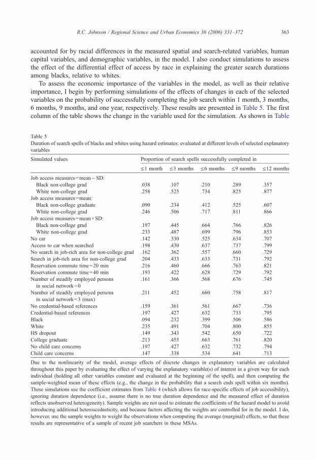
R.C. Johnson / Regional Science and Urban Economics 36 (2006) 331–372 363
accounted for by racial differences in the measured spatial and search-related variables, human
capital variables, and demographic variables, in the model. I also conduct simulations to assess
the effect of the differential effect of access by race in explaining the greater search durations
among blacks, relative to whites.
To assess the economic importance of the variables in the model, as well as their relative
importance, I begin by performing simulations of the effects of changes in each of the selected
variables on the probability of successfully completing the job search within 1 month, 3 months,
6 months, 9 months, and one year, respectively. These results are presented in Table 5. The first
column of the table shows the change in the variable used for the simulation. As shown in Table
Table 5
Duration of search spells of blacks and whites using hazard estimates: evaluated at different levels of selected explanatory
variables
Simulated values Proportion of search spells successfully completed in
V1 month V3 months V6 months V9 months V12 months
Job access measures=mean�SD:
Black non-college grad .038 .107 .210 .289 .357
White non-college grad .258 .525 .734 .825 .877
Job access measures=mean:
Black non-college graduate .090 .234 .412 .525 .607
White non-college grad .246 .506 .717 .811 .866
Job access measures=mean+SD:
Black non-college grad .197 .445 .664 .766 .826
White non-college grad .233 .487 .699 .796 .853
No car .142 .330 .525 .634 .707
Access to car when searched .198 .430 .637 .737 .799
No search in job-rich area for non-college grad .162 .362 .557 .660 .729
Search in job-rich area for non-college grad .204 .433 .633 .731 .792
Reservation commute time=20 min .216 .460 .666 .763 .821
Reservation commute time=40 min .193 .422 .628 .729 .792
Number of steadily employed persons
in social network=0
.161 .366 .568 .676 .745
Number of steadily employed persons
in social network=3 (max)
.211 .452 .660 .758 .817
No credential-based references .159 .361 .561 .667 .736
Credential-based references .197 .427 .632 .733 .795
Black .094 .232 .399 .506 .586
White .235 .491 .704 .800 .855
HS dropout .149 .343 .542 .650 .722
College graduate .213 .455 .663 .761 .820
No child care concerns .197 .427 .632 .732 .794
Child care concerns .147 .338 .534 .641 .713
Due to the nonlinearity of the model, average effects of discrete changes in explanatory variables are calculated
throughout this paper by evaluating the effect of varying the explanatory variable(s) of interest in a given way for each
individual (holding all other variables constant and evaluated at the beginning of the spell), and then computing the
sample-weighted mean of these effects (e.g., the change in the probability that a search ends spell within six months)
These simulations use the coefficient estimates from Table 4 (which allows for race-specific effects of job accessibility)
ignoring duration dependence (i.e., assume there is no true duration dependence and the measured effect of duration
reflects unobserved heterogeneity). Sample weights are not used to estimate the coefficients of the hazard model to avoid
introducing additional heteroscedasticity, and because factors affecting the weights are controlled for in the model. I do
however, use the sample weights to weight the observations when computing the average (marginal) effects, so that these
results are representative of a sample of recent job searchers in these MSAs.
.
,
,
R.C. Johnson / Regional Science and Urban Economics 36 (2006) 331–372364
5, the differential effects of job accessibility by race contribute significantly to the black–white
gap in search durations. A one standard deviation increase in both job accessibility measures from
their respective mean values increases the probability of successfully completing the job search
spell within six months by .252 (61.2%) for black non-college graduates, while not significantly
affecting the probability for whites. Thus, these simulated results imply that a spatial redistribution
of jobs that gives blacks high accessibility to employment opportunities will considerably narrow
the black–white gap in average search duration, no matter what effect the spatial redistribution has
on whites’ present job accessibility. As previously discussed, this result is likely because whites
face far fewer residential location constraints and thus are more residentially mobile.
How do the effects of changes in job accessibility compare with changes in other explanatory
variables? As shown in Table 5, we see large effects among the other spatial search related
variables. Access to a car while searching increases the probability of successfully finding a job
and ending search within six months by .112 (21.3%). Searching in a job-rich area increases the
probability of successfully finding a job and ending search within six months by .076 (13.6%)
for non-college graduates. In contrast, simulating an increase in reservation commute time from
20 to 40 min decreases the probability of successfully finding a job and ending search within six
months by .038 (5.7%). Simulating an increase in social network quality from poor to good
social networks (proxied by simulating change from not having any individuals in immediate
social network with a steady job to having all the individuals in immediate social network with
steady jobs) increases the probability of successfully finding a job and ending search within six
months by .092 (16.2%). Having credential-based references increases the probability of
successfully completing a job search within six months by .071 (12.7%). Being black decreases
probability of successfully completing a job search within six months by .305 (43.3%). Among
the selected human capital and demographic variables, we see somewhat smaller effects.
Simulating an increase in education from less than 12 years (high school dropout) to 16 years or
more (college graduate) increases the probability of successfully finding a job and ending search
within six months by .121 (22.3%). Having child care concerns decreases the probability of
successfully completing the job search within six months by .098 (15.5%).
7.5. Decomposition analysis: accounting for racial differences in search outcomes
The large black–white gap in the hazard of successfully completing a job search (.040 versus
.072—ignoring duration dependence, these transition rates imply average search durations of
24.8 weeks for blacks and 13.9 weeks for whites) can be decomposed into two parts: (1) the gap
due to racial differences in the distributions of individual characteristics, and (2) the gap due to
racial differences in the returns of job accessibility (likely stemming from racial differences in
residential location constraints) and unexplained racial differences (which may reflect labor
market discrimination and/or the inability to include unmeasurable variables). I employ a
variation of the Blinder–Oaxaca decomposition method developed by Fairlie (1999) to estimate
the proportion of the black–white gap in the hazard of successfully completing a job search that
can be explained by differences in spatial and search related characteristics, human capital
characteristics, and demographic characteristics.
For a linear regression, the standard Blinder–Oaxaca decomposition of the black–white gap in
the average value of the dependent variable, Y, can be expressed as
YW � Y
B ¼ XW � X
B�bBiþ X
W�bW � bB
�i;
h�h
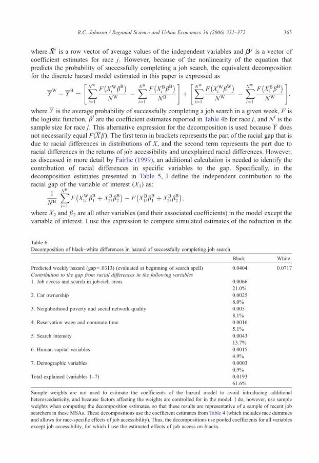
R.C. Johnson / Regional Science and Urban Economics 36 (2006) 331–372 365
where Xj is a row vector of average values of the independent variables and bb j is a vector of
coefficient estimates for race j. However, because of the nonlinearity of the equation that
predicts the probability of successfully completing a job search, the equivalent decomposition
for the discrete hazard model estimated in this paper is expressed as
YW � Y
B ¼XNW
i¼1
F XWi bB
� �NW
�XNB
i¼1
F X Bi bB
� �NB
#þ
XNW
i¼1
F XWi bW
� �NW
�XNW
i¼1
F X Bi bB
� �NW
#;
""
where Y is the average probability of successfully completing a job search in a given week, F is
the logistic function, bj are the coefficient estimates reported in Table 4b for race j, and Nj is the
sample size for race j. This alternative expression for the decomposition is used because Y does
not necessarily equal F(Xb). The first term in brackets represents the part of the racial gap that is
due to racial differences in distributions of X, and the second term represents the part due to
racial differences in the returns of job accessibility and unexplained racial differences. However,
as discussed in more detail by Fairlie (1999), an additional calculation is needed to identify the
contribution of racial differences in specific variables to the gap. Specifically, in the
decomposition estimates presented in Table 5, I define the independent contribution to the
racial gap of the variable of interest (X1) as:
1
NB
XNB
i¼1F XW
1i bB1 þ X B
2ibB2
� �� F X B
1ibB1 þ X B
2ibB2
� �;
where X2 and b2 are all other variables (and their associated coefficients) in the model except the
variable of interest. I use this expression to compute simulated estimates of the reduction in the
Table 6
Decomposition of black–white differences in hazard of successfully completing job search
Black White
Predicted weekly hazard (gap= .0313) (evaluated at beginning of search spell) 0.0404 0.0717
Contribution to the gap from racial differences in the following variables
1. Job access and search in job-rich areas 0.0066
21.0%
2. Car ownership 0.0025
8.0%
3. Neighborhood poverty and social network quality 0.005
8.1%
4. Reservation wage and commute time 0.0016
5.1%
5. Search intensity 0.0043
13.7%
6. Human capital variables 0.0015
4.9%
7. Demographic variables 0.0003
0.9%
Total explained (variables 1–7) 0.0193
61.6%
Sample weights are not used to estimate the coefficients of the hazard model to avoid introducing additiona
heteroscedasticity, and because factors affecting the weights are controlled for in the model. I do, however, use sample
weights when computing the decomposition estimates, so that these results are representative of a sample of recent job
searchers in these MSAs. These decompositions use the coefficient estimates from Table 4 (which includes race dummies
and allows for race-specific effects of job accessibility). Thus, the decompositions use pooled coefficients for all variables
except job accessibility, for which I use the estimated effects of job access on blacks.
l
R.C. Johnson / Regional Science and Urban Economics 36 (2006) 331–372366
black–white transition rate gap that would result from giving blacks the same distribution of X1
as possessed by whites, while holding the distribution of the other variables constant. I replicate
this procedure substituting a different variable of interest for X1 to estimate the contribution of
each variable to the gap.33
Table 6 reports estimates from this procedure for decomposing the black–white gap in
the hazard of successfully completing a job search. These results provide estimates of
the reduction in the black–white transition rate gap resulting from giving blacks the
same distribution of all included variables as whites, as well as the relative
contributions of specific subsets of variables to the gap. The contribution estimate
indicates that racial differences in all included variables of the model account for
roughly two-thirds of the gap. As shown in Table 6, examination of racial differences
in specific subsets of variables reveals that racial differences in job accessibility play an
important role in explaining the transition rate gap. The contribution estimate indicates
that racial differences in job accessibility and the extent of search in job-rich areas
account for 21%. The results indicate that if blacks were given the car ownership rates
of whites, the transition rate gap would be reduced by 8%. The other spatial and
search related variables contribute to the gap as well. Racial differences in neighborhood
poverty and social network quality account for 8.1% of the gap. Racial differences in
reservation commute time and wage account for 5.1%; and racial differences in the
distribution of search intensity account for 13.7% (although it is important to note,
these differences may have arisen endogenously). In sum, the contribution estimates
indicate that the cumulative effects of racial differences in the spatial search-related
variables account for roughly 40% of the black–white gap. In contrast, despite the large
differences between blacks and whites in levels of education and work experience, differences
in human capital and demographic characteristics explain a much smaller part of the gap—6%.
This result is mainly due to the weaker relationship between education and job search
duration.
8. Summary and policy implications
This paper provides strong evidence supporting the spatial mismatch hypothesis, which
states that involuntary housing segregation discourages the search for or acceptance of jobs at
workplaces far from workers’ residences. This restricts the racial group’s employment
opportunities and makes them more sensitive to local labor market demand conditions. The
inconsistency of the results of previous studies that have attempted to test the spatial mismatch
hypothesis, and the resulting controversy concerning the relevance of space in explaining
racial differences in labor market outcomes, is a byproduct of the use of imprecise/
33 These calculations, however, are not possible without first matching the white distribution of X1 and the black
distribution of X2. I follow the procedure used by Fairlie (1999) to match these distributions. Specifically, using the
coefficient estimates reported in Table 4, I calculate predicted probabilities for all observations in the white sample and all
observations in a random subsample of blacks with sample size equal to NW, since the black sample is slightly larger than
the white sample (NB=409NNW=313, resulting from the over-sampling of blacks). I draw a large number of random
black subsamples (1000 random subsamples of blacks of size 313) and present the mean value of estimates from these
samples. I rank each member of the two samples by the value of this predicted probability and match them by their
respective ranks. This procedure assigns low transition probability blacks the same characteristics as low transition
probability whites.
R.C. Johnson / Regional Science and Urban Economics 36 (2006) 331–372 367
inappropriate measures of job accessibility. The detailed geographic measures of job
accessibility developed in this paper are an important contribution to the analysis of spatial
issues examined in this study. I show that the geographic areas within each MSA that were
relatively rich in employment opportunities for non-college graduates were not only located in
predominantly white suburbs more than 10 mi from the centroid of black residential
concentration, but were also areas that were not served by public transportation (exacerbating
spatial mismatch).
There are significant race differences in the effects of job accessibility. The role of
residential segregation in constraining blacks’ and Hispanics’ residential location choices
appears to be the source of the differential effect of access by race. Simulation
results show that blacks’ greater sensitivity to local labor market demand conditions
contribute significantly to the black–white gap in search durations. In addition, racial
differences in the distribution of job accessibility and the extent of search in job-rich
areas account for one-fifth of the black–white gap in the hazard of successfully
completing a job search, and the cumulative effect of racial differences in all the
included spatial search-related variables accounts for roughly 40% of the overall
black–white gap.
The results of this study suggest that greater enforcement of fair housing laws, as well
as policies that alter the distribution of jobs in metropolitan areas in favor of the central
city – such as empowerment zones, combined with full employment policies that tighten
labor markets–will significantly improve blacks’ and Hispanics’ job search outcomes. The
present findings on the role of job accessibility and dimensions of job search have
important policy implications for the success of welfare reform, as PRWORA’s work
requirements and participation mandates have led most states and localities to implement
programs focused on job search assistance. The analysis also provides some micro
foundations to the aggregate trends of demand shifts and population adjustments
documented by Bound and Holzer (1980), who report that differential responses to local
demand shifts across groups, as well as the geographic distribution of the shifts themselves,
help to account for the regional pattern of inequality that developed in the 1980s. This
research has sought to analyze the mechanisms through which a worker’s location within
the economy affects his/her return to human capital, and to identify the processes that
hinder a smooth adjustment to changing labor market conditions. Further analysis is needed
along these lines.
Appendix A. Estimating the distance decay function
Gravity models (often referred to as spatial interaction models) have been used extensively in
the urban transportation literature to model commuting patterns (Isard, 1960; Sen and Smith,
1995; Fotheringham, 1989). Using CTPP data (designed for transportation planners) on journey-
to-work flows between neighborhoods in the Atlanta, Boston, and Los Angeles MSAs, I model
the extent of commuting between every possible neighborhood (origin (i)-destination (j)) pair as
a function of the number of workers that live in neighborhood i (Li); the number of jobs located
in neighborhood j (Ej); the accessibility of job location j to all alternative job locations available
(Aj); the occupational/skill compatibility between workers that live in neighborhood i and
neighborhood j-jobs (occij); and the distance in miles between neighborhoods i and j (dij) and
cost of overcoming this distance (captured by the distance decay function, Fij). I estimate the

R.C. Johnson / Regional Science and Urban Economics 36 (2006) 331–372368
aggregate commute flow of labor from an origin to a destination neighborhood by the gravity
equation
Tij ¼ KLai E
bj A
dj exp /occij
� �Fij; ð1Þ
where Tijunumber of workers that live in neighborhood i and work in neighborhood j; Fij
(distance decay function)=exp[c1 (dij)+c2 (dij*plinci)]; plinciu% of workers that live in
neighborhood i that earn less than $25,000/year; and K, a, b, d, /, c1, c2 are parameters to be
estimated. Equivalently, if we use lower-case letters to denote the logarithms of variables
denoted by corresponding capital letters (e.g., ln Ai=ai), we can write the gravity model (1) as
tij ¼ k þ ali þ bej þ daj þ /occij þ c1 dij� �
þ c2 dijTplinci� �h i
: ð1VÞ
As the dependent variable in Eq. (1) is the count of workers that commute between given
neighborhoods, estimation requires the use of an econometric model that takes the dependent
variable as being generated from a discrete probability process (Greene, 1993; Raphael, 1998). I
estimate Eq. (1) with a negative-binomial count model. A negative-binomial regression equation
can be written as:
Yi ¼ expXi¼1
biXi
!þ e;
where Yi follows a negative-binomial distribution whose expected value is equal to
exp�P
i¼1biXi
�; equivalently, the natural logarithm of Yi is equal to the linear predictor. Thus,
in the gravity model case, the negative-binomial regression equation becomes:
Tij ¼ exp k þ ali þ bej þ daj þ /occij þ c1 dij� �
þ c2 dijTplinci� �� �� �
þ ei: ð1WÞ
The origin labor supply (Li) and the destination labor demand (Ej) capture the possible scale
of interaction between the two neighborhoods. By entering labor supply and demand
multiplicatively in the gravity equation, the potential scale of interaction increases in the total
possible combinations of worker–job matches, with a, b N0 (Raphael, 1998).
It is also important to control for the configuration of competing job location destinations—
i.e., the destination neighborhood’s proximity to all other job location destinations. Aj reflects
the competition between location j and all alternative job locations for commuting flows
(workers). As the accessibility of a job location to all alternative job locations increases, we
expect the commuting volume to that job location to decrease, other things being equal
(Fotheringham, 1989)—thus, d b0. I use the following measure for the proximity of a
destination to all others:
Aj ¼XKk¼1
Ek
djk
�:
�
Obviously, if a residential neighborhood has all blue-collar employees, there would not be
many people from that neighborhood holding jobs in a predominantly white-collar area. Ideally,
one would construct a separate model for each occupational/skill category, but the necessary data
R.C. Johnson / Regional Science and Urban Economics 36 (2006) 331–372 369
are not available. Therefore, I take the approach used previously by Soot and Sen (1991) to
construct an occupational/skill compatibility index. Let pi(1),. . ., pi
(7) be the proportion of
employees in each of seven employment categories living in i, and let qj(1),. . ., qj
(7) be the
proportion of jobs in each category employed in j. Following Soot and Sen (1991), I define the
occupational compatibility index as
occij ¼XMm¼1
ffiffiffiffiffiffiffiffip
mð Þi
q ffiffiffiffiffiffiffiffiq
mð Þj
q #:
"
By the Cauchy-Schwartz inequality (Rao, 1973),
" XMm¼1
ffiffiffiffiffiffiffiffip
mð Þi
q ffiffiffiffiffiffiffiffiq
mð Þj
q #VXMm¼1
pmð Þi
" #1=2 XMm¼1
qmð Þj
" #1=2¼ 1;
with the equality holding if and only if pi(m) =qj
(m) for all m. Thus, (occij)=1 when the match is
bperfectQ (i.e., pi(m) =qj
(m) for all m (employment categories)), and equal to zero when the match is
essentially nonexistent (i.e., pi(m) qj
(m) =0 for all m (employment categories)), and increases with
improving matches. The occupational/skill compatibility index entered as in Eq. (1) implies the
aggregate flow of labor between given neighborhoods increases proportionately with the degree
of occupational compatibility between workers and jobs in the given neighborhoods (/ N0). The
seven occupational categories used were (a) professional, executive, administrative, and
managerial, (b) technicians and related support, (c) sales, (d) administrative support (including
clerical), (e) service, (f) precision products, craft, and repair, and (g) operators, fabricators, and
laborers.
Of primary interest is the estimation of the distance decay parameters (c1,c2) of the distancedecay function (Fij). The specific functional form of the decay function in Eq. (1) is a more
general form of the function often used in transportation planning models (Sen and Smith, 1995)
and implies that the aggregate flow of labor declines proportionately with distance (c1b0).Ideally, we would like to model the commuting patterns of low-wage or less-educated workers
separately, since commuting patterns differ by earnings/skill, but disaggregated commuting flow
data by earnings or education levels are not available. Consequently, when modeling the
relationship between observed commuting patterns and distance, it is important to control for the
average earnings of neighborhood workers since the commuting patterns of low-wage workers
tend to be more localized than those of high-wage earners (for reasons discussed elsewhere).
Spatial search theoretic models predict the attenuating effect of distance on low-wage workers’
search and commute patterns to be greater than that for high-wage workers (Simpson, 1992).
Thus, I interact the percent of workers that live in neighborhood i that earn less than $25,000 per
year with the measure of distance between neighborhood i and j. This interaction variable
(dij*plinci) effectively assigns a larger distance decay parameter (in absolute value) when the
origin neighborhood is composed of a larger percentage of workers that have low earnings—that
is, c2b0. Given the high level of earnings homogeneity within neighborhoods, due to residential
segregation by income, I argue c =c1+c2 provides a good estimate of the distance decay
parameter for less-skilled workers. Thus, the estimated distance decay function for low-wage
workers is Fij =exp(cdij) and captures the composite effects of distance in reducing their
probability of searching/finding/accepting distant job offers.

R.C. Johnson / Regional Science and Urban Economics 36 (2006) 331–372370
Appendix A.1. Gravity model estimation results
Using the negative-binomial count model for the gravity equation yielded an estimated distance
decay parameter for less-skilled workers of� .101 in Atlanta,� .149 in Boston, and � .093 in theLos Angeles MSA. As expected, the estimated distance decay parameters for higher income
workers are smaller in magnitude (in absolute value), reflecting more spatially expansive search/
commute patterns (relative to lower income workers). The estimated distance decay parameter for
higher income workers is � .073 in Atlanta, � .063 in Boston, and � .046 in Los Angeles. As
previously discussed, the estimated distance decay function is used to weight nearby jobs
(competing workers) more than distant jobs (competing workers). Thus, using our estimated
distance decay parameter for less-skilled workers in Atlanta, jobs (competing workers) located at
distances of 0, 5, 10, 15, and 20mi would have weights of 1, .60, .36, .22, and .13, respectively. The
effects of the other explanatory variables of the gravity equation were all significant and in the
expected directions. These first-stage estimation results are shown in Appendix Table A. I chose
not to estimate race-specific distance decay parameters because I did not want to confound the
effects of race and space inherently in the construction of my job accessibility measures.
Table A
Gravity model estimates from negative binomial regressions: Atlanta, Boston, and Los Angeles MSA commute patterns
Dependent variable Atlanta Boston Los Angeles
Number of workers that live in neighborhood
i and work in neighborhood j
coefficient estimate coefficient estimate coefficient estimate
ln(Li) .8930*** .7488*** � .1766***ln(Ej) .8420*** .7502*** .0607***
ln(Aj) � .1817*** � .2999***Occij 52.7205*** 87.5901*** 337.0598***
Distanceij (mi) � .0728*** � .0626*** � .0459***Distanceij*plinc25i � .0283*** � .0868*** � .0470***Total distance decay parameter for lower income workers � .1011*** � .1493*** � .0929***
Constant �9.216*** �6.3433*** .8728***
ln(alpha) 2.8124*** 2.7498*** 3.3280***
Log-likelihood �571,389.93 �605,522.6N 794,988 744,769 267,029
***p b .01.
Li =the number of workers that live in neighborhood i.
Ej =the number of jobs located in neighborhood j.
Aj =the accessibility of job location j to all alternative job locations available.
Occij =the occupational/skill compatibility between workers that live in neighborhood i and neighborhood j-jobs.
dij =the distance in miles between neighborhoods i and j.
plinc25i =% of workers that live in neighborhood i that earn less than $25,000/year. I tried alternative threshold levels for
low earnings—e.g., % of workers that live in neighborhood with earnings less than $20,000 ($30,000)—but none
significantly altered the estimate of the distance decay parameter.
There are 892 zones in Atlanta. This results in a 892�892 matrix of commuting flows for Atlanta.
There are 863 zones in Boston. This results in a 863�863 matrix for Boston.
There are 1653 in Los Angeles. This results in a 1653�1653 matrix for Los Angeles. Because of computer memory
limitations, the negative binomial model was estimated 10 times with a separate 10% sample for the Los Angeles gravity
estimates.

R.C. Johnson / Regional Science and Urban Economics 36 (2006) 331–372 371
Acknowledgment
I am grateful to John Bound, Charlie Brown, Sheldon Danziger, Harry Holzer, and Ted
Mouw for detailed comments and helpful discussions; to Sheldon Danziger and Harry Holzer for
access to the restricted-use versions of the MCSUI surveys; and Ted Mouw for sharing programs
that greatly assisted me in constructing my job accessibility measures. This paper also benefited
from the comments of Richard Arnott, John Quigley, Steven Raphael, two anonymous referees,
and participants of the conference on Urban Change and Spatial Mismatch (Chicago Federal
Reserve Bank) and the University of Michigan Labor seminar. This research was supported by
funding received from the Ford Foundation and the University of Michigan Rackham Graduate
School.
References
Arnott, Richard, 1998. Economic theory and the spatial mismatch hypothesis. Urban Studies 35 (7), 1171–1185 (June).
Bound, John, Holzer, Harry J., 2000. Demand shifts, population adjustments, and labor market outcomes during the
1980s. Journal of Labor Economics 18 (1), 20–54.
Brueckner, J.K., Zenou, Yves, 2003. Space and unemployment: the labor market effects of spatial mismatch. Journal of
Labor Economics 21, 242–266.
Coulson, Edward, Laing, Derek, Wang, Paul, 2001. Spatial mismatch in search equilibrium. Journal of Labor Economics
19 (4), 949–972 (October).
Ellwood, David T., 1986. The spatial mismatch hypothesis: are there teenage jobs missing in the ghetto?
In: Freeman, Richard B., Holzer, Harry (Eds.), The Black Employment Crisis. University of Chicago Press, Chicago,
pp. 147–190.
Erickson, Rodney, Wasylenko, Michael, 1980. Firm location and site selection in suburban municipalities. Journal of
Urban Economics 8, 69–85.
Fairlie, Robert, 1999. The absence of the African-American owned business: an analysis of the dynamics of self-
employment. Journal of Labor Economics 17 (1), 80–108 (January).
Fotheringham, Stewart, 1989. Spatial Interaction Models: Formulas and Applications. Kluwer Academic, Boston.
Greene, William H., 1997. Econometric Analysis. Prentice-Hall, Upper Saddle River, NJ.
Holzer, Harry J., 1987. Informal job search and black youth unemployment. American Economic Review 77, 446–452
(June).
Holzer, Harry J., 1988. Search method use by unemployed youth. Journal of Labor Economics 6 (1), 1–20.
Holzer, Harry J., 1996. What Employers Want: Job Prospects for Less-Educated Workers. Russell Sage Foundation, New
York.
Holzer, Harry J., Ihlanfeldt, Keith R., 1996. Spatial factors and the employment of blacks at the firm level. New England
Economic Review, 65–82 (May/June).
Holzer, Harry J., Ihlanfeldt, Keith R., Sjoquist, David L., 1994. Work, search and travel among white and black youth.
Journal of Urban Economics 35, 320–345 (May).
Hughes, Mark, Sternberg, Julie, 1992. The New Metropolitan Reality: Where the Rubber Meets the Road in Antipoverty
Policy. The Urban Institute Press, Washington, D.C.
Iceland, John, Weinberg, Daniel H., Steinmetz, Erika, 2002. Racial and Ethnic Residential Segregation in the United
States, 1980–2000. U.S. Census Bureau, Special Report Series, CENSR #3.
Ihlanfeldt, Keith R., 1997. Information on the spatial distribution of job opportunities within metropolitan areas. Journal
of Urban Economics 41, 218–242 (March).
Isard, W., 1960. Methods of Regional Analysis: An Introduction to Regional Science. The Technology Press of MIT,
New York.
Johnson, Rucker C., 2004. Landing a Job in Urban Space: The Extent and Effects of Spatial Mismatch. Longer web
version of published paper downloadable at: http://socrates.berkeley.edu/~ruckerj/SMHRSUE.pdf.
Kain, John F., 1968. Housing segregation, Negro employment and metropolitan decentralization. Quarterly Journal of
Economics 82 (3), 175–197.
Kasarda, John D., 1985. Urban change and minority opportunities. In: Peterson, Paul (Ed.), The New Urban Reality.
Brookings Institute, Washington, DC.
R.C. Johnson / Regional Science and Urban Economics 36 (2006) 331–372372
Kasarda, John D., 1995. Industrial restructuring and the changing location of jobs. In: Farley, Reynolds (Eds.), State of
the Union vol. 1. Russell Sage Foundation, New York, pp. 33–68.
Katz, Lawrence, Kling, J., Liebman, J., 2001. Moving to opportunity in Boston: early results of a randomized mobility
experiment. Quarterly Journal of Economics 116 (2), 607–654.
Massey, Douglass, Denton, Nancy, 1992. American Apartheid. Harvard University Press, Cambridge.
Mouw, Ted, 2000. Job relocation and the racial gap in unemployment in Detroit and Chicago 1980–1990: a fixed-effects
estimate of the spatial mismatch hypothesis. American Sociological Review 65, 730–753 (October).
Mouw, Ted, 2002. Are black workers missing the connection? The effect of spatial distance and employee referrals on
interfirm racial segregation. Demography 39 (3), 507–528.
O’Regan, Katherine M., Quigley, John M., 1996. Spatial effects on employment outcomes: the case of New Jersey
teenagers. New England Economic Review (Federal Reserve Bank of Boston), pp. 41–57. May/June Special Issue.
Rao, C.R., 1973. Linear Statistical Inference and its Applications. Riley, New York.
Raphael, Steven, 1998. The spatial mismatch hypothesis and black youth joblessness: evidence from the San Francisco
bay area. Journal of Urban Economics 43, 79–111.
Rogers, Cynthia L., 1997. Job search and unemployment duration: implications for the spatial mismatch hypothesis.
Journal of Urban Economics 42, 108–132.
Sen, Ashish, Smith, T.E., 1995. Gravity Models of Spatial Interaction Behavior. Springer-Verlag, New York.
Simpson, Wayne, 1992. Urban Structure and the Labor Market. Oxford University Press, New York.
Soot, Siim, Sen, Ashish, 1991. A spatial employment and economic development model. Papers in Regional Science 70,
149–166.
Stephenson Jr., Stanley P., 1976. The economics of youth job search behavior. The Review of Economics and Statistics
58 (1), 104–111.
Stoll, Michael A., Holzer, Harry J., Ihlanfeldt, Keith R., 2000. Within cities and suburbs: racial residential concentration
and the spatial distribution of employment opportunities across sub-metropolitan areas. Journal of Policy Analysis
and Management 19 (2), 207–231 (Spring).
Wasylenko, Michael, 1984. Disamenities, local taxation, and the intrametropolitan location of households and firms. In:
Ebel, Robert (Ed.), Research in Urban Economics, vol. 4. JAI Press, Greenwich, CT.
Wilson, William Julius, 1987. The Truly Disadvantaged: The Inner City, the Underclass and Public Policy. University of
Chicago Press, Chicago.
Wilson, William Julius, 1996. When Work Disappears: The World of the New Urban Poor. Alfred A. Knopf, New York.
Yinger, John, 1986. Measuring discrimination with fair housing audits: caught in the act. American Economic Review 76,
881–893 (December).
Yinger, John, 1995. Closed Doors, Opportunities Lost: The Continuing Costs of Housing Discrimination. Russell Sage
Foundation, New York.
Zax, Jeffrey S., Kain, John F., 1996. Moving to the suburbs: do relocating companies leave their black employees
behind? Journal of Labor Economics 14 (3), 473–504.