land use, sedimentation, and marine resource vulnerability ... · ridge to reef land use,...
TRANSCRIPT

Ridge to Reef
Land Use, Sedimentation, and Marine Resource Vulnerability in Raja Ampat, Indonesia
Team Members: Brandon Doheny
Katy Maher Andrew Minks Jeremy Rude
Marlene Tyner
Faculty Advisor: Thomas Dunne
A group project submitted in partial satisfaction of the degree requirements for the Master of Environmental Science & Management
March 22, 2013

Ridge to Reef: Land Use, Sedimentation, and Marine Resource Vulnerability in Raja Ampat, Indonesia
As authors of this Group Project report, we are proud to archive this report on the Bren School’s website such that the results of our research are available for all to read. Our signatures on the document signify our joint responsibility to fulfill the archiving standards set by the Bren School of Environmental Science & Management.
BRANDON DOHENY
KATY MAHER
ANDREW MINKS
JEREMY RUDE
MARLENE TYNER
The mission of the Bren School of Environmental Science & Management is to produce professionals with unrivaled training in environmental science and management who will devote their unique skills to the diagnosis, assessment, mitigation, prevention, and remedy of the environmental problems of today and the future. A guiding principal of the School is that the analysis of environmental problems requires quantitative training in more than one discipline and an awareness of the physical, biological, social, political, and economic consequences that arise from scientific or technological decisions.
The Group Project is required of all students in the Master’s of Environmental Science and Management (MESM) Program. It is a three-quarter activity in which small groups of students conduct focused, interdisciplinary research on the scientific, management, and policy dimensions of a specific environmental issue. This Final Group Project Report is authored by MESM students and has been reviewed and approved by:
THOMAS DUNNE
MARCH 2013

iii
Table of Contents
List of Figures .......................................................................................................................................... v
List of Tables ......................................................................................................................................... vii
Acknowledgements ........................................................................................................................... viii
Abstract ................................................................................................................................................... ix
Executive Summary .............................................................................................................................. 1
I. Project Significance ..................................................................................................................... 5
II. Project Objectives ......................................................................................................................... 6
III. Background ................................................................................................................................ 8 A. Geography, Climate, and Topography............................................................................... 8 B. Hydrodynamic Conditions in Raja Ampat ....................................................................... 9 C. Marine Resources................................................................................................................... 10
Coral Reefs .................................................................................................................................................. 10 Marine Protected Areas ......................................................................................................................... 11 Dive Sites...................................................................................................................................................... 11 Pearl Farms ................................................................................................................................................. 12
D. Socioeconomic Factors ......................................................................................................... 12 E. Land use Change in Raja Ampat ........................................................................................ 13 F. Land use Change and Erosion Rates ................................................................................ 14 G. Biological Impacts of Erosion ............................................................................................ 15
Erosion and Coral Reefs ......................................................................................................................... 15 Erosion and Fisheries ............................................................................................................................. 15
H. Erosion Modeling ................................................................................................................... 16 I. Sediment Plume Modeling .................................................................................................. 16
IV. Methodology ............................................................................................................................ 18 A. Terrestrial Model ................................................................................................................... 19
Overview ...................................................................................................................................................... 19 Factors .......................................................................................................................................................... 20
B. Marine Model ........................................................................................................................... 32 Overview ...................................................................................................................................................... 32 Inputs ............................................................................................................................................................ 32 Sediment Extent Model .......................................................................................................................... 40
C. Vulnerability Analysis .......................................................................................................... 42 Data Sources ............................................................................................................................................... 42 Analysis ........................................................................................................................................................ 42
V. Results ............................................................................................................................................ 43 A. Terrestrial Results ................................................................................................................. 43
Current Land Use ...................................................................................................................................... 43 Conservative Land use Change Scenario ......................................................................................... 46 Intensive Land use Change Scenario ................................................................................................. 50
B. Marine Model Results ........................................................................................................... 54 Sediment Extent Model Results .......................................................................................................... 54 Vulnerability Analysis Results ............................................................................................................. 61

iv
VI. Discussion ................................................................................................................................. 61 A. Terrestrial Model ................................................................................................................... 61
Limitations and Uncertainty ................................................................................................................ 63 B. Marine Sediment Extent Model ......................................................................................... 65
Limitations and Uncertainty ................................................................................................................ 67 C. Vulnerability Analysis .......................................................................................................... 69
VII. Conclusions .............................................................................................................................. 70 A. The Model as a Framework ................................................................................................ 70 B. Suggestions for Further Research .................................................................................... 70
References ............................................................................................................................................. 72
Appendix – Sensitivity Analysis for Suspension Maintenance Factor and Settling Rates ........................................................................................................................................................ 79

v
List of Figures
Figure 1. Map of marine resources in the Raja Ampat region ............................................................. 6
Figure 2. Political Map of Raja Ampat ........................................................................................................... 8
Figure 3. Map of Raja Ampat ............................................................................................................................. 9
Figure 4. Recent road development on Waigeo looking over Kabui Bay and the resulting sediment plumes. Photographs by James Morgan. ............................................................................... 14
Figure 5. Conceptual description of the coupled terrestrial and marine tool ............................ 18
Figure 6. Slope and Length-Slope factors ................................................................................................. 22
Figure 7. Waigeo land use and C factors ................................................................................................... 25
Figure 8. Batanta (N) and Salawati (S) land use and C factors ......................................................... 26
Figure 9. Average annual precipitation (mm) and R factor using (Lo et al. 1985) method . 28
Figure 10. Soil erodibility nomograph (Tew 1999) .............................................................................. 30
Figure 11. K factor using Tew (1999) method........................................................................................ 31
Figure 12. Interpolation of HYCOM surface currents for final surface current layer .............. 33
Figure 13. Final bathymetry layer components ..................................................................................... 35
Figure 14. Final bathymetry layer ............................................................................................................... 35
Figure 15. Revised settling rate .................................................................................................................... 37
Figure 16. Horizontal relative moving angle (HRMA) parameter (ESRI 2012) ......................... 39
Figure 17. Horizontal factor (HF) parameter (ESRI 2012) ................................................................ 39
Figure 18. Path Distance layer results ....................................................................................................... 40
Figure 19. Overview of Sediment Extent Model ..................................................................................... 41
Figure 20. Annual sediment loss per hectare under current land use .......................................... 44
Figure 21. Annual sediment loss per watershed under current land use .................................... 45
Figure 22. Annual sediment loss per hectare under the conservative land use change scenario .................................................................................................................................................................. 47
Figure 23. Annual sediment loss per watershed under the conservative land use change scenario .................................................................................................................................................................. 48
Figure 24. Gag Island soil loss rates resulting from mining activities ........................................... 49
Figure 25. Difference in annual sediment loss per watershed between the current and conservative land use change scenario ..................................................................................................... 49
Figure 26. Annual sediment loss per hectare under the intensive land use change scenario ................................................................................................................................................................................... 51
Figure 27. Annual sediment loss per watershed under the intensive land use change scenario .................................................................................................................................................................. 52

vi
Figure 28. Difference in annual sediment loss per watershed under the intensive land use change scenario .................................................................................................................................................. 53
Figure 29. Total annual soil loss under each land use scenario ....................................................... 53
Figure 30. Annual SEM results under current land use in 2011 ...................................................... 54
Figure 31. SEM results on northern Waigeo under current land use ............................................ 56
Figure 32. SEM results for Batanta and Salawati under current land use ................................... 56
Figure 33. SEM results under the conservative land use change scenario .................................. 57
Figure 34. SEM results under all land use scenarios for Gag Island and Waisai on southern Waigeo .................................................................................................................................................................... 59
Figure 35. SEM results under all land use scenarios for Batanta .................................................... 60
Figure 36. Watershed sensitivity to land use .......................................................................................... 63
Figure 37. SEM results for Batanta and Salawati under current land use (shown for the month of February) ........................................................................................................................................... 66
Figure 38. SEM results for Batanta and Salawati under current land use (shown for the month of July) ...................................................................................................................................................... 67

vii
List of Tables
Table 1. Size and management institutions for MPAs in Raja Ampat ............................................ 11
Table 2. Value of Raja Ampat’s main economic sectors ...................................................................... 12
Table 3. C Factor literature review .............................................................................................................. 24
Table 4. Ordinal categories of soil erosion potential............................................................................ 43
Table 5. Marine resources within 2011 SEM plume extents ............................................................. 61
Table 6. Average soil erosion rates for land use classes between land use scenarios ............ 62
Table 7. Watersheds losing high amounts of soil between land use scenarios ......................... 62

viii
Acknowledgements
This project would not have been possible without the guidance, expertise, and support of others. It is with deep gratitude that we acknowledge the contributions of the following people: Faculty Advisor: Thomas Dunne, Bren School of Environmental Science & Management, UCSB External Advisors: Sarah Lester, Marine Science Institute, UCSB James Frew, Bren School of Environmental Science & Management, UCSB Client: Conservation International Hedley Grantham Christine Huffard Ismu Hidayat Others: Libe Washburn, Marine Science Institute, UCSB Ben Halpern, National Center for Ecological Analysis and Synthesis Eric Treml, University of Melbourne Alex Messina, San Diego State University Eric Fournier, Bren School of Environmental Science & Management, UCSB Aubrey Dugger, Bren School of Environmental Science & Management, UCSB Alex Valencourt Chuck Schonder
ix
Abstract Sediment erosion associated with changes in land use are considered one of the greatest anthropogenic threats to coral reef ecosystems. To assess the vulnerability of high-value marine resources to sedimentation in Raja Ampat, Indonesia, we developed a coupled terrestrial and marine model that predicts the relative quantities of sediment at river mouths for current and future land use change scenarios, and the spatial extent over which this sediment disperses in the ocean. The terrestrial model routes sediment loads predicted by a Revised Universal Soil Loss Equation (RUSLE) to river mouths, and the Sediment Extent Model (SEM) maps the maximum plume extents based on the effects of surface currents, depth, and particle settling rates on sediment dispersal. The combined output of these two models is sediment loading (kg m-2) within the plumes. To illustrate the utility of the model, we calculated sediment loss under two hypothetical land use change scenarios: a conservative one in which sediment loads increased by 13%, and an intensive one in which loads increased by 47%. In total, the SEM predicted 1,987 km2 of coral reefs, marine protected areas, dive sites, pearl farms, and other benthic habitats in Raja Ampat to lie within the sediment plumes, although not enough is known about the effects of sedimentation on these resources to convert predictions of sedimentation into biological impacts. The model provides a powerful visual tool that conservation planners can use to communicate how land use change may impact high-value marine resources to Indonesian decision makers and other local stakeholders. However, the model should be improved with high-resolution near-shore data to more accurately predict sediment movement and dispersal within the ocean.

1
Executive Summary Background Raja Ampat is a group of islands located in Indonesia’s Western Papua province. The region encompasses over four million hectares of land and sea and includes the four large islands of Waigeo, Batanta, Salawati and Misool, and hundreds of smaller islands. As part of the Coral Triangle region, Raja Ampat is a biologic hotspot and a global priority for marine conservation. The region is home to the highest marine biodiversity on the planet, with three-quarters of the world’s hard coral species, and over 1,300 coral reef fish species (Dive Raja Ampat 2010; Erdmann and Pet 2002). The region’s rich terrestrial and marine resources have made it a target for development. Land use change often increases erosion, heightening concerns about increased sediment yields from island watersheds. High levels of sedimentation can have deleterious effects on coral reef ecosystems (Richmond 1993; Rogers 1990), meaning development choices on land could negatively impact biodiversity in the ocean. This biodiversity supports the majority of the economic sectors of the region, meaning land development could have huge implications on the sustainability of economic growth in the area. Objectives Our client, Conservation International (CI), has therefore asked us to broadly assess the relative vulnerability of marine resources to sedimentation from land use changes. To do this, we sought to answer the following questions: (1) which watersheds have the potential to contribute to sedimentation, (2) which marine resources are currently at risk from land use-driven sedimentation, and (3) how might land use change influence sediment loading? To answer these questions, we identified the main objectives of our research:
Predict sediment yields to river mouths resulting from current land use and two example land use change scenarios
Map the marine areas at risk of sedimentation extending from each river mouth Identify the extent of each marine resource that overlaps with potential
sedimentation zones, including coral reefs, marine protected areas (MPAs), dive sites, and pearl farms.
To do this, we developed a novel coupled terrestrial and marine model that predicts the output of sediment to river mouths under three land use scenarios, and maps the spatial extent of marine sediment dispersal. The terrestrial component of our model takes predictions of watershed sediment yields made by a Revised Universal Soil Loss Equation (RUSLE) and routes them to the river mouths on all the major islands of the region. The marine component maps the maximum plume extents based on the effects of surface currents, depth, and particle settling rates on sediment dispersal.

2
Methodology – Terrestrial Model We modeled terrestrial soil loss using RUSLE for both current land use and two hypothetical land use change scenarios. RUSLE consists of a set of factors which represent the contribution of varying soil erosion drivers to an estimated long-term annual amount of soil loss per unit area. There are five contributing factors to the soil loss equation: the rainfall erosivity factor represents the erosion potential from rainfall, the soil erodibility factor represents the effect of soil characteristics, the slope-length and slope-steepness factors collectively represent the effect of topography, and the cover management factor indicates the effect of vegetation cover and land use. Each of these factors was determined on the basis of multiple regression equations, calibrated to field measurements in various regions. RUSLE produced tonnes of soil lost per year per hectare, which we then translated into the total amount of sediment exiting each river mouth annually for over 600 individual watersheds in the region. Although we illustrated its use for the case of long-term average annual conditions, the method can be used for predictions of extremely wet years or for individual wet months in climates with a strong seasonality of rainfall. In addition to estimating soil loss under current land use, we created two example land use change scenarios, guided by regional development plans and consultation with knowledgeable people from the region. The conservative land use change scenario models urban growth, agricultural development, and mining activities on slopes primarily less than 20°. The intensive land use change scenario models similar, yet slightly exaggerated development patterns in areas regardless of slope. It is important to note that these scenarios are not meant to predict future land uses in any way, nor do they provide any recommendations for sustainable development, but are rather used to illustrate the utility of the soil erosion model and reveal how various land uses affect soil erosion in different topographic regions. Methodology – Marine Model The Sediment Extent Model (SEM) was developed to assess the maximum extent over which sediment would disperse into the ocean from river mouths as a function of surface currents, water depth, and particle settling velocities. In the SEM, currents act as the driving force for horizontal movement, while settling rates drive the vertical movement of the particles. These factors are combined with bathymetry to produce the maximum extent of sediment plumes from each river mouth. To model the furthest extent of each plume, we used the settling rate of the finest sediment class, silt and clay. To compensate for near-shore dynamics, such as wave energy and bathymetric influences not captured by available current data, we modified the settling rate as an inverse function of water depth. The settling rate coupled with the horizontal particle travel time due to currents tracks the trajectory of a sediment particle at any time period as it moves away from a river mouth and sinks. We then subtracted particle depth from ocean depth at every cell to determine the extent of sediment plumes. If this equation results in a positive number, we know that the sediment has not yet settled out completely. The moment that this value becomes either zero or negative, the sediment has arrived at the ocean floor and the smallest particles in that
3
plume have settled out of solution. It is this boundary that reflects the maximum extent of a sediment plume. We ran the SEM for every month in the year 2011 to produce 12 monthly plume extents. Because the model cannot predict the spatial pattern of sedimentation along each flow trajectory, we divided the total sediment loads for each month from river mouth by the monthly plume extent and then summed the plumes to obtain an index of sedimentation intensity within the plumes. This was the final output for our SEM. Results Under current land use, annual sediment supply at individual river mouths ranged from 8 to 131,000 t yr-1. River mouths predicted to release relatively high sediment loads generally were correlated with larger watersheds. The highest sediment loads emanate from northern Waigeo and western Misool. Other watersheds yielding relatively high amounts of sediment are found on northwestern Waigeo, eastern Mayalibit Bay, Manuran Island, Gebe Island, and the greater Sorong region. Conservative Land use Change The conservative land use change scenario resulted in approximately a 13% increase in the calculated amount of sediment entering the ocean. Mining is the primary cause for increases of extreme soil erosion potential, due to the presence of mineable mineral resources, particularly on Gag Island and the northern coast of Waigeo. This scenario illustrates the potential impact of development in areas where the slopes are primarily less than 20°. Therefore, the majority of agriculture development, urban growth, and road expansion resulted in low to moderate impacts on erosion potential. Some urban growth, specifically near Waisai, had high impacts on erosion potential. Overall, relatively few watersheds had large increases of sediment loss between current and conservative land use change scenarios. Intensive Land use Change The intensive land use change scenario resulted in a 47% increase in the total amount of sediment entering the ocean. In this scenario, several mines are placed throughout northern Waigeo, Kawe Island, and Gag Island on slopes greater than 20°, causing extreme soil erosion potential. Other contributing land use changes that resulted in high to extreme erosion rates included urban growth and road development. These types of development were modeled to occur more often on steeper slopes in this scenario, which exacerbated average soil erosion rates for these land uses. Vulnerability Analysis The SEM results predicted that 1,987 km2 of Raja Ampat will be affected by sediment loads to the ocean, mostly in near-shore coastal habitats. Plume extents were greatest in areas with strong currents and deep water, including around Sayang, Gebe, and Gag Islands, as well as the southwestern coast of Misool, and the channel between Batanta and Salawati. However, greater extents of the plume translate into lower indices of sedimentation intensity in our model and would include those areas where the currents are too fast and the wave energy too high to allow sedimentation. A vulnerability analysis showed that 57

4
km2 of coral reefs, 479 km2 of MPAs, 4 dive sites, 1 pearl farm, and 1,930 km2 of other benthic habitats lie within these sediment plume extents and could be impacted by sedimentation. Limitations In conducting our analysis, we identified several limitations of each of the models used. For example, the soil loss predictions indicate only spatial variations in relative soil loss rates and their sensitivity to land use change. We do not attempt to predict the exact amount of sediment that will reach a river mouth. Instead we predict relative soil loss across the region to identify areas where soil loss is vulnerable to disturbances. The SEM takes into account only the far-field surface current speed, calculated from regional conditions. It does not take into account near-shore modifications of current speed or direction, waves, or tides. The currents used in the SEM were from a global database, which does not contain a sufficiently high resolution to provide an accurate depiction of near-shore processes. In particular, currents impinging orthogonally on a river mouth will not allow the model to distribute sediment along the coast, confining sedimentation instead into unnaturally small areas of very high sedimentation intensity. Improvements in defining near-shore currents will improve the utility of the SEM at these locations, but were outside of the scope of our investigation. Conclusions We developed a coupled terrestrial and marine model to assess how land use changes impact the amount of sediment entering the ocean and determine where that sediment is dispersed. This tool made it possible to assess the vulnerability of the region’s marine resources to increases in sedimentation to be expected from example land use change scenarios, thereby specifically addressing the needs of CI. The tool is flexible in terms of spatial and temporal extent and can be applied to a variety of other planning processes. Our tool can be refined with improved local data, including more accurate land cover (and predicted land use change), as well as fine-scale oceanographic characteristics. In addition, the tool is adaptable to seasonality considerations for erosion and currents. The tool could be used to focus on sedimentation during rainy months or during periods of the year when currents have the potential to carry sediment further out into the ocean. This tool is an important first step in helping visualize the linked effects of land erosion and ocean impacts, but there is still work to be done. There are two main ways to improve the model’s functionality. The most influential improvement would be to obtain and use high resolution current data in the near-shore environment that accurately represents long-shore current movement. Another way would be to alter interpolated HYCOM or other coarse-scale data so that it approximates this effect within the modeling environment. The tool would be most useful to land use planning efforts after these issues are addressed. In addition, land use planning efforts will consider important economic and biological effects along with sedimentation impacts. We recommend further research on the biological and economic linkages between sedimentation and key marine resources to provide a more comprehensive understanding of how land use change impacts the marine environment to land use planners and other stakeholders.

5
I. Project Significance The coral reefs in Raja Ampat are invaluable for their rich biodiversity, which include more than 600 hard coral species. Hard corals are foundation species that create habitat and food for more than 1,300 reef fish species and many other marine invertebrates that contribute to the resilience and productivity of local and regional waters (Dive Raja Ampat 2010; Wilkinson 2004; Donnelly et al. 2002). Major convergence currents cool the local waters and circulate nutrients, protecting the region thus far from bleaching effects and other impacts associated with climate change. Raja Ampat is a key biodiversity sanctuary that generates, maintains, and disperses genetic diversity across large geographic areas of the Indo-West Pacific (Salm and Mcleod 2008). Coral health is inextricably linked to the productivity of MPAs, and the economic yields of tourism and fisheries (Cesar 2002). The natural resources from coastal waters are the basis for a subsistence economy upon which the majority of the human population in Raja Ampat directly depends (Donnelly et al. 2002). Ultimately, the livelihoods of local communities and the integrity of biodiversity within and adjacent to Raja Ampat depend upon the survivability of coral reefs. Sediment in runoff caused by changes in land use is among the greatest anthropogenic threats to coastal coral reefs (Rogers 1990; Richmond et al. 2007; Wilkinson 2004). Future land use changes in Raja Ampat, Indonesia, threaten to increase sedimentation rates, which may lead to coral reef smothering and subsequent reductions in biodiversity and fishery stocks (Rogers 1990; Fabricius 2005). These land use changes are expected to include the expanding mining and logging operations, a developing tourism industry, and population growth (Bailey and Pitcher 2008; Donnelly et al. 2002).
Conservation managers have recognized the need to identify potential land use impacts on marine resources. This analysis focuses on identifying the vulnerability of coral reefs, dive sites, marine protected areas (MPAs), and pearl farms in the Raja Ampat region (Figure 1) to terrestrial sediment yields. We developed a coupled terrestrial and marine model that both predicts the output of sediment to river mouths under various land use scenarios, and then maps the maximum extent of marine sediment dispersal from these river mouths. By identifying the vulnerable marine resources throughout the region, we provide a tool that facilitates more effective simulation of development options for decision makers in Raja Ampat. The tool provides a first step in coupling land and sea interactions, enabling managers to be more informed when making complicated decisions concerning long term planning for marine conservation.

6
Figure 1. Map of marine resources in the Raja Ampat region
II. Project Objectives The overall objective of this project is to provide Conservation International (CI), the Indonesian government, and the local communities of the Raja Ampat region with an assessment of the vulnerability of coral reefs, dive sites, MPAs, and pearl farms to sedimentation from land use changes. To meet this objective, we sought to answer three research questions:
1. Which watersheds have the potential to contribute to sedimentation?
2. Which marine resources are currently at risk from land use-driven sedimentation?
3. How might land use change influence sediment loading?

7
To answer these questions, we identified the main objectives of our research:
Predict sediment yields to river mouths resulting from current land use and two example land use change scenarios
Map the marine areas at risk of sedimentation extending from each river mouth
Identify the extent of each marine resource that overlaps with potential sedimentation zones, including coral reefs, MPAs, dive sites, and pearl farms.
It is important to note that the example land use change scenarios do not represent predictions of land use change in the region, nor do they provide any recommendations for sustainable development. They are simply meant to illustrate how the tool can be used to examine changes in land use, and how this may impact marine resources in the region. This information will be used by local land managers in conjunction with other stakeholders to better understand the spatial dynamics of where current land use and proposed land use changes will impact the marine environment.

8
III. Background
Figure 2. Political Map of Raja Ampat
A. Geography, Climate, and Topography
The Raja Ampat region of Indonesia, also known as the Bird’s Head Seascape, lies at the center of the Coral Triangle (Figure 3). The Coral Triangle encompasses areas rich in marine biodiversity and includes parts of Indonesia, the Philippines, Malaysia, and Papua New Guinea (McKenna et al. 2002). Raja Ampat includes the four large islands of Waigeo, Batanta, Salawati, and Misool and hundreds of smaller islands. This area encompasses over 43,000 square kilometers or four million hectares of land and sea (Donnelly et al. 2002). The islands lie at the northeastern entrance of the Indonesian Throughflow, a strong current system that flows from the Pacific Ocean to the Indian Ocean (Donnelly et al. 2002).
Raja Ampat experiences the dry and wet periods that are characteristic of tropical islands. The dry season extends from October through March, while the wet season is usually April

9
through September, with June and July the wettest months (McKenna et al. 2002). Average monthly precipitation during the dry season is 17 centimeters, while during the wet season the average monthly precipitation is 27 centimeters (McKenna et al. 2002).
The Raja Ampat islands are characterized by karst topography, with elevations ranging from sea level up to 1,000 meters (McKenna et al. 2002). Terrestrial habitats on the islands are diverse, and include submontane forest, scrub, beach forest, sago swamps, and mangroves (Webb 2005). The coastal environments within the region range from sheltered bays to shorelines exposed to the open (McKenna et al. 2002).
B. Hydrodynamic Conditions in Raja Ampat
The natural location and shape of the Raja Ampat islands largely dictates the predominant surrounding oceanographic conditions. The islands are scattered across the equator at the confluence of the western Pacific Ocean and eastern Indian Ocean. Oceanographic patterns are extremely complex in this area (Agostini et al. 2012). The “Indonesian Throughflow” is the driver of most large-scale current patterns, and is generated by the passage of water from the Pacific Ocean southward through the archipelago into the Indian Ocean (Agostini et al. 2012). This creates a general oceanic current flowing from the northeast to the southwest in the region (Treml 2008). A strong clockwise eddy to the west (the Halmahera eddy) also impacts Raja Ampat (Agostini et al. 2012). The passage of strong currents through the myriad small islands and reefs then creates many local eddies and turbulence which can vary seasonally (Agostini et al. 2012). Seasonal changes can also weaken or reverse the general current movement, particularly impacting northern islands during the northwest monsoon season (Erdmann and Pet 2002; Treml 2008).
There are two distinct seasonal influences on Raja Ampat, the southeast monsoon from May-October and the northwest monsoon from November-March. Winds are generally from the southeast between May and October, and mainly from the northwest between December and March. Between these months, winds are generally light as meteorological conditions transition (McKenna et al. 2002).
Figure 3. Map of Raja Ampat
10
In Raja Ampat, tides are mixed with weak semi-diurnal tides being the dominant type.
(Palomares and Heymans 2006). The maximum daily tide fluctuation is approximately 1.8 m, with an average daily fluctuation of about 0.9-1.3 m. Periodic strong currents are common throughout the area, especially in channels between islands. These currents can be affected by the monsoons, moving generally eastward in the west monsoon and westward in the east monsoon (Palomares and Heymans 2006). Average current speeds have been recorded at 2.32 km hr-1, with top speeds of 4.63 km hr-1 (Palomares and Heymans 2006). Sea temperatures generally hover around 19-36°C and severe thermoclines or areas of upwelling are not common (McKenna et al. 2002; Agostini et al. 2012).
C. Marine Resources
As part of the Coral Triangle region, Raja Ampat is known for its high concentration of marine biodiversity. The high diversity of marine habitats in Raja Ampat –ranging from fringing, barrier, patch and atoll reefs to deep channels between the main islands – contributes to this high biodiversity (Agostini et al. 2012). The area has many important marine resources, including coral reefs, MPAs, dive sites, and pearl farms.
Coral Reefs
Fringing and platform reefs support the majority of coral species in Raja Ampat. The variable shapes of shorelines throughout the region create different types of exposure for fringing reefs. These types of reefs are found in open sea areas, as well as in highly sheltered bays and inlets. Many coral reefs are found along the northern coast of Batanta and on the western side of Waigeo, which both have many sheltered bays. Mayalibit Bay, the large sheltered bay on Waigeo, has some coral reefs toward the southern end of the inlet and within the narrow channel separating the bay from the ocean (McKenna et al. 2002).
Recent surveys in the Raja Ampat region have recorded over 1,300 species of coral reef fishes and over 600 species of the order Scleractinia, or stony coral, which represent approximately 70% of the global coral reef species diversity. One study found that 96% of all Scleractinian coral recorded within Indonesia are likely to occur in the Raja Ampat Islands (McKenna et al. 2002). The area has the world’s highest coral reef biodiversity per unit land area (Dive Raja Ampat 2010). One study found an average of 87 species of coral per site surveyed. This study found that relatively exposed fringing reefs support the highest number of coral species in the region, though platform reefs and sheltered bays also support high numbers of coral species. The area surrounding Batanta was found to have the highest number of corals per site surveyed (McKenna et al. 2002).
The coral reefs within the region are currently in very good condition, mainly due to low levels of natural disturbances and low levels of human development. Compared to other areas of Indonesia, coral reefs in Raja Ampat have high live coral diversity and minimal stress from natural phenomenon such as cyclones, predation (i.e. crown-of-thorns starfish), and freshwater runoff (McKenna et al. 2002). In addition, the abundance of large coral colonies in Raja Ampat suggests that the region has not suffered from the mass coral bleaching events that many other tropical areas have (Erdmann and Pet 2002).
11
Marine Protected Areas
MPA is a term that can be used to describe marine reserves, fishery reserves, closed areas, no-take areas/zones, sanctuaries, parks, wilderness areas, and locally managed areas. MPAs are designed to support ecosystem health, productivity, and to contribute to social and economic development. The management of MPAs can range from community-managed areas to multi-million hectare national parks (Smith et al. 2009). In the Coral Triangle region, MPAs are generally managed as either fully protected areas where extractive activities are prohibited (such as fishing), or as multiple use areas where various different types of activities are permitted (Agostini et al. 2012).
There are currently seven MPAs in Raja Ampat (Figure 1), which vary in size and management jurisdiction (Table 1). Prior to 2007, the Raja Ampat MPA (located in southwest Waigeo) was the only protected area. The MPA network was expanded through the creation of six additional MPAs by the Raja Ampat Regency government in 2007. The seven MPAs in the Raja Ampat region now cover a total of over 1 million hectares (Agostini et al. 2012; Wiadnya et al. 2011).
The MPA network is governed by the Raja Ampat Regency and the Ministry of Marine Affairs and Fisheries with support from conservation organizations (such as CI and The Nature Conservancy (TNC)) and the Coral Reef Rehabilitation and Management Program (COREMAP), which is run by the government of Indonesia. The Raja Ampat government is currently developing management and zoning plans for several of the MPAs with support from CI, TNC, and World Wildlife Fund (WWF) (Agostini et al. 2012).
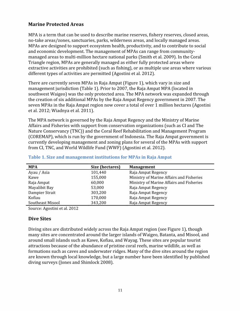
Table 1. Size and management institutions for MPAs in Raja Ampat
MPA Size (hectares) Management
Ayau / Asia 101,440 Raja Ampat Regency Kawe 155,000 Ministry of Marine Affairs and Fisheries Raja Ampat 60,000 Ministry of Marine Affairs and Fisheries Mayalibit Bay 53,000 Raja Ampat Regency Dampier Strait 303,200 Raja Ampat Regency Kofiau 170,000 Raja Ampat Regency Southeast Misool 343,200 Raja Ampat Regency
Source: Agostini et al. 2012
Dive Sites
Diving sites are distributed widely across the Raja Ampat region (see Figure 1), though many sites are concentrated around the larger islands of Waigeo, Batanta, and Misool, and around small islands such as Kawe, Kofiau, and Wayag. These sites are popular tourist attractions because of the abundance of pristine coral reefs, marine wildlife, as well as formations such as caves and underwater ridges. Many of the dive sites around the region are known through local knowledge, but a large number have been identified by published diving surveys (Jones and Shimlock 2008).

12
Pearl Farms
Pearl farming contributes over $4.5 million each year to the Raja Ampat economy (Table 2). Several pearl farming companies have had operations in Raja Ampat since the 1990s. Cendana Indopearl, a subsidiary of the Australian pearl company Atlas South Sea Pearl, has had several farms off Waigeo since the mid-1990s. Many of these farms are within Alyui Bay (Atlas South Sea Pearl Limited 2013). The company holds concession agreements with local communities for a given coordinate with a 500 meter radius. For each concession, the contract is 30 years. One study estimates that by the year 2000, these farms had a total of 600,000 oysters and had harvested 36,000 pearls (Smith and Anastasi 2009). In addition, Raja Ampat Mariculture, a family-owned pearl farm, has two farms in Raja Ampat (Raja Ampat Mariculture LLC 2012).
D. Socioeconomic Factors
According to a 2001 census, the Raja Ampat islands have a population of approximately 50,000 people (UNESCO 2003). The islands are located close to Sorong, a large coastal city located to the east on the main island of Papua New Guinea (McKenna et al. 2002). Close to 80% of the people who live in the Raja Ampat Regency derive their main source of income from coral reef fisheries (Smith et al. 2009). Most of the local Raja Ampat people are subsistence fishermen, though there is a small amount of commercial fishing and live reef fish trade (McKenna et al. 2002; McLeod et al. 2009). Tourism is also an important activity in Raja Ampat, with many people visiting the area to access the region’s unique dive sites. However, the contribution of tourism to the Raja Ampat economy is relatively low. Much of the tourism revenue goes directly to Sorong, the primary base from which most diving expeditions depart (Bailey and Pitcher 2008). There has been an effort to incorporate dive fees at Raja Ampat dive sites, which enables this revenue to go directly to the local government (Bailey and Pitcher 2008). The values of the various economic sectors in Raja Ampat are presented in Table 2 below.
Table 2. Value of Raja Ampat’s main economic sectors
Sector Billion Indonesian Rupiah Million US$ Artisanal fisheries 63.1 7.01 Pearl farming 41.0 4.56 Commercial fisheries 20.5 2.28 Agriculture 14.8 1.64 Tourism 14.4 1.60 Logging 12.2 1.36 Reef gleaning 2.2 0.244 Mining 1.7 0.189 Other marine 0.023 0.0026 TOTAL VALUE 169.9 18.89
Source: Bailey and Pitcher 2008 Note: Values are converted from Indonesian Rupiah (IDR) to US dollars (US$) using the conversion rate of 9000 IRD to $1 US

13
E. Land use Change in Raja Ampat
Despite its small population, Raja Ampat is experiencing habitat destruction by activities such as logging, illegal fishing activities, mining, and development of roads and urban areas (McKenna et al. 2002). Figure 4 shows pictures of road development contributing to erosion of sediments, which are deposited into marine areas. The forest industry in Raja Ampat has been dominated by collaborative arrangements between the leadership of local communities, government officials, military and police, and local timber companies. Despite these collaborative agreements, instances of logging and forest destruction have occurred in both protected and non-protected areas of Raja Ampat (Donnelly et al. 2002). In addition to deforestation, land use changes for mining development are also a concern for Raja Ampat. BHP Billiton, the largest mining company in the world, has been given rights to mine on one of the islands. Sedimentation and toxic runoff from mines could pose major risks to marine resources (Bailey and Pitcher 2008). As marine biodiversity is incredibly sensitive to changes in its environment, understanding the threat of land use driven sedimentation to the Raja Ampat region of Indonesia is of critical importance. Erosion is controlled by a combination of rainfall, topographic steepness, vegetation cover, and soil type, as well as land use practices that may exacerbate or conserve soil loss (El-Swaify et al. 1982). Relatively flat land covered with thick vegetation within dry climates will erode less than steeply-sloped areas in wet climates with minimal vegetation. Under the latter conditions, the soil is not stabilized by plant roots and therefore high rainfall and the gravitational effect of loose material perched on a steep slope will work together to carry the soil to lower elevations. Tropical mountainous islands are particularly susceptible to erosion because they are characterized by high precipitation and steep slopes. Additionally, high population densities of low-income people under pressure to clear land for subsistence farming or other economic uses exacerbate this susceptibility (El-Swaify et al. 1982).

14
Figure 4. Recent road development on Waigeo looking over Kabui Bay and the resulting sediment plumes. Photographs by James Morgan.
F. Land use Change and Erosion Rates
Human-driven land use changes such as deforestation and conversion of land to agriculture generally accelerate erosion rates due to the increased exposure of soils to interaction with rainfall and slope. Land use changes may have an enormous impact on the erosion rates of tropical islands. In the U.S. Virgin Islands, the addition of 50 km of roads caused four times the island-wide sedimentation than natural rates (MacDonald et al. 1997). In Micronesia, land use such as forest clearing and farming increased sediment yields in a river catchment
15
to 150 tons square kilometers per year compared to the 1.9 tons square kilometers per year found in a pristine river catchment (Victor et al. 2004).
G. Biological Impacts of Erosion
Erosion and Coral Reefs Increased sedimentation loads to the coasts of tropical islands have extensive negative impacts on natural marine environments. High sedimentation loads smother coral reefs, typically killing them within a few hours of burial, and deter larvae from reef settlement (Rogers 1990; Fabricius 2005; Edinger et al. 1998; Babcock and Smith 2000). Larval settlement rates are practically zero on sediment-covered surfaces, and overall, reduce the growth and survival of many coral species (Fabricius 2005). Specific effects of high sedimentation loading onto corals include reductions in radial growth, live coral presence, coral larvae recruitment, calcification, and net primary productivity, as well as increased branching growth (Rogers 1990). Increased sedimentation may also have indirect negative effects on coral health. High sediment loads may allow some species of algae to persist where coral species cannot, increasing the strength of interspecies competition between algae and corals and thus the stress on already-weakened corals (Nugues and Roberts 2003). Indonesian reefs are not immune to these effects. Mean suspended sediment concentrations in reefs not subject to human activity was reported to be less than 10 milligrams per liter, and mean sediment influx rates less than 1 to 10 milligrams per square centimeter per day (Rogers 1990). However, for several reefs surrounding the islands of Java and Ambon, mean suspended sediment concentrations ranged from 4 to 29 milligrams per liter, and mean sediment influx rates were measured as high as 32 milligrams per square centimeter per day (Holmes et al. 2000). Another study found that sewage, industrial pollution, and sediment influx to the coasts of six study sites throughout Indonesia decreased coral biodiversity 40-60% in shallow depths where currents are more likely to carry sediments away (Edinger et al. 1998). However, we were not able to find information relating rates and frequency of sedimentation to the intensity of coral reef degradation, and so were not able to convert our own estimates of sedimentation intensity into calculations of biological risk.
Erosion and Fisheries
Increased sedimentation loads negatively impacting coral reefs, mangroves, and seagrass beds can partially explain the overall decline in tropical fisheries (Rogers 1990). Sedimentation weakens corals by compromising structural integrity. As coral structures collapse and die, habitat availability among the corals decreases, limiting both the number of fish species the coral reef can support as well as the number of individuals (Rogers 1990). In the Eastern Caroline Islands, the number of fish species significantly decreased near a runway construction site that emitted fine silts and sediments into the water. As a result, fish numbers declined 50-100% with increasing sediment loads on reef surfaces (Amesbury 1981). Decreases in stock may significantly impact local and national economies.

16
H. Erosion Modeling
A variety of models exist for estimating soil loss and sediment transport. These models range in their complexity, data requirements, and capabilities. In general there are three main categories of soil erosion models. These include empirical, conceptual, and physically based models. Physically-based models are centered on equations describing streamflow and sediment generation in a catchment. This type of modeling requires large amounts of data, and is not viable for large areas. Conceptual models are based on the representation of lumped processes over the scale at which the outputs are simulated. They usually incorporate the underlying transfer mechanisms of sediment and runoff generation. Conceptual models tend to include a general description of catchment processes, without including the specific details of process interactions, which would require detailed catchment information. While useful for describing erosion events and relationships, they do not allow quantitative comparisons and predictions to be made. Lastly, empirical models are based primarily on the analysis of observations at sample sites, and seek to characterize generalized responses from these data. The computational and data requirements for such models are usually less than for physically-based models, allowing them to be supported by coarse measurements. Empirical models are used for making projections of land use effects in preference to more complex models as they can be implemented in situations with limited data and parameter inputs, and are particularly useful as a first step in identifying sources of sediment generation (Merritt et al. 2003). Due to data limitations in Raja Ampat, an empirically based model was chosen for estimating terrestrial soil erosion. The Universal Soil Loss Equation (USLE) is an empirical overland flow sheet-rill erosion regression equation. Its outputs are both temporally and spatially lumped, providing an average annual estimate of soil erosion from hillslopes. The original intention of the USLE was to estimate soil loss on agricultural lands. However, over time the equation has been modified to accommodate a broader range of landscapes and land cover types. The most well-known modification to the USLE is the Revised Universal Soil Loss Equation (RUSLE). RUSLE came about as a necessary improvement to USLE, allowing for the model’s use in a digital interface (Renard et al. 2011). Since then, many functional forms of RUSLE have arisen (Nearing 1997; Tew 1999; Lo et al. 1985) to meet the varying needs of its practitioners. Through these variations RUSLE has been extended to estimate soil erosion on a multitude of landscapes with varying soil types, topography, precipitation patterns, and vegetation cover. RUSLE was chosen because of its relatively low data requirements, the conceptually robust form of the equations, and its ability to be applied utilizing a geographic information system.
I. Sediment Plume Modeling
Sediment plume modeling is a challenging endeavor that may be conducted at several levels of complexity using a variety of methods. Simple, explanatory models have been developed using localized in situ measurements to characterize plumes in small near-shore sites (Su and Wang 1989; Wolanski et al. 2003; Golbuu et al. 2003). Plumes have also been assessed using remotely sensed data gathered using aerial imagery (Hill et al. 2000; Curran et al. 2002) and satellites (Baban 1995; Tassan 1997; Ruhl et al. 2001; Choi et al. 2012). Finally, complex numerical models have been developed that take into account various

17
oceanographic processes such tidal forcing, sea surface height, surface wind stress, ocean temperature and salinity, bathymetry, and near-shore flows and eddies. For example, ADCIRC (ADvanced CIRCulation Model for Oceanic, Coastal and Estuarine Waters) (Luettich et al. 1992), a numerical model that takes into account the previously listed parameters, has been used to model larval dispersion nearby, in the Bird’s Head Seascape (Treml 2008). Other fine-scale numerical models take into account additional processes such as fine-sediment flocculation, inter-grain friction, and freshwater forcing (Liu et al. 2002).
Because ADCIRC was implemented in the Bird’s Head Seascape at the behest of stakeholders who overlap with this effort, we explored the option to implement ADCIRC for this project. However, ADCIRC is a highly complex numerical model that requires a high level of technical expertise, time, and computing power, resources to which we did not have access. In addition, Treml (2008) found that the bathymetry and currents data which the ADCIRC model requires is not available for the region. The needs and capabilities of our clients on-the-ground in Raja Ampat are similar to our own group, and so developing an ADCIRC-based product for them would not be useful to them in terms of future implementation efforts. Therefore, we decided to develop a novel, generalized method to estimate and visualize the overall risk to marine resources using the best available data and modeling tools available to the Raja Ampat team.

18
IV. Methodology CI requested that we evaluate the relative impacts of sediment yields from current and future land uses in Raja Ampat on coral reefs, MPAs, dive sites, and pearl farms. To accomplish this, a coupled terrestrial and marine tool was developed to link sediment loadings on land to the spatial distribution of sediment in the ocean (Figure 5). Terrestrial sediment yields were first modeled from the watersheds of Raja Ampat to individual river mouths. The dispersal of those materials in the ocean was then modeled. Finally, we identified the areas of sediment dispersal that affected coral reefs, dive sites, MPAs, and pearl farms. To demonstrate the utility of this tool, the sediment model was run for various land use scenarios, including the current land use in the region and two example future land use change scenarios. These example land use change scenarios do not represent predictions of land use change in the region, nor do they provide any recommendations for sustainable development. They are simply meant to illustrate how the tool can be used to examine changes in land use, and how this may impact marine resources in the region.
Figure 5. Conceptual description of the coupled terrestrial and marine tool

19
A. Terrestrial Model
Overview
The terrestrial model uses RUSLE to estimate annual soil loss from each river mouth in Raja Ampat. Those soil loss estimates were then summed and translated to their associated river mouths. The monthly proportion of annual soil loss was then estimated at each river mouth utilizing an equation derived from the modified Fournier’s Index (Arnoldus 1980). The RUSLE estimates average annual soil loss from a unit area and can be represented as the following equation. Equation 1.
Where A is the estimated soil loss per unit area, R is the rainfall erosivity factor, K is the soil erodibility factor, L is the slope-length factor, S is the slope-steepness factor, C is the cover and management factor, and P is the support practices factor (Wischmeier and Smith 1978). Each factor is generated by a different algorithm, outlined in the following sections. RUSLE Model Implementation The RUSLE model was implemented using ArcGIS version 10.1. This was done through a raster analysis, where each factor was represented as a grid of cells which covered the entire region of interest (ROI). Each cell represented a 90 meter by 90 meter square (8,100 m2) within the ROI. Each cell can only have one value associated with it for each factor. The algorithms outlined in the previous section were used to populate the values in the cells, after which the grids were multiplied together to obtain an annual amount of soil loss for each cell in tonnes of soil lost per year per hectare. We then corrected this value to each cell by multiplying the cell value by 0.81, as the area of our cell size corresponds to 81% of a hectare. This then produced the annual soil loss per cell. We then spatially summed the cell grid based on the watershed they were associated with. This produced an annual soil loss per watershed. This value then was transferred to the river mouths for each watershed, giving the total amount of sediment exiting each river mouth per year. It was assumed that all soil loss occurring on the terrestrial landscape was transferred to river mouths. This assumption was made because the catchments in Raja Ampat are generally steep, with narrow river valleys, and fine grain sediment. The combination of these factors precludes long-term sediment storage along the water courses of these islands. Watershed Delineation The first step in conducting any kind of hydraulic modeling, including sediment transport, is delineating streams and watersheds, and obtaining some basic watershed properties such as area, slope, flow accumulation, as well as other watershed characteristics. Generating these datasets is known as terrain pre-processing. With the availability of ArcGIS and digital elevation models (DEMs) these properties were derived through an automated process. Specifically, the Arc Hydro toolset was utilized, an extension available

20
for use with ArcGIS (Arc Hydro Toolset). To conduct the terrain pre-processing we used ArcGIS 10.1. The DEM used to conduct the watershed delineation was obtained online from the CGIAR Consortium for Spatial Information (CGIAR-CSI 2013). The dataset was derived from the Shuttle Radar Topographic Mission (SRTM) 90m digital elevation data for the entire world. The SRTM digital elevation data, produced by the National Aeronautics and Space Administration (NASA) originally, is a major breakthrough in digital mapping of the world, and provides a major advance in the accessibility of high quality elevation data for large portions of the tropics and other areas of the developing world (CGIAR-CSI 2013). The SRTM DEM was downloaded in four separate DEMs. In order to begin processing the data they had to be mosaicked together using ArcGIS. We then clipped the combined DEM to our region of interest. The first step in processing the DEM was to fill all the sinks in the dataset. That is, any areas where water would get trapped had to be elevated to a point where that would no longer occur. This is done using the Fill Sinks tool. The next step was to determine the flow path along the terrain using the Flow Direction tool. Next was calculating the number of grid cells that flow into any given cell in the DEM using the Flow Accumulation tool. At this point there was enough information to define streams within our study area. The Stream Definition tool allows you to choose exactly what the threshold of flow accumulation is which defines a stream. A threshold of 100 cells was chosen, or an area of 810,000 m2. Any cells which have a flow accumulation of 100 or more would then be considered part of the stream network for our study area. The next step was to use the Stream Segmentation tool; this function creates a grid of stream segments that have a unique identification. From the output of the Stream Segmentation tool we can then define catchments using the Catchment Grid Delineation tool. There is essentially one catchment created for every stream segment. Next, a vector layer for streams was created using the Drainage Line Processing tool. Additionally, a vector layer for catchments was created using the Catchment Polygon Processing tool. Lastly, drainage points for each catchment were created using the Drainage Point Processing tool. These points represent where tributaries feed into larger streams and eventually where river mouths let out into the ocean.
Factors
LS Factor
Literature Review
The slope-length factor (L) and the slope-steepness factor (S) are most often combined into a single term known as the length-slope topographic factor (LS). There are more questions and concerns about the length-slope topographic factor than for any other term in RUSLE. This is largely due to the complexities of representing these factors within the raster format of a GIS. The two main questions that arise when determining the Length-Slope factor are how to represent the downslope runoff path of an area and how to define that area in terms of slope length and steepness (Renard et al. 2011).

21
Data
The same DEM used in the watershed delineation was used in calculating the length-slope factor (LS).
Methods
To calculate the length-slope factor (LS) first several data sets had to be derived from the DEM. These datasets included slope angle in degrees, percent-rise, and radians. To calculate the slope-length factor (L) the equation suggested by McCool, Foster, and Weesies (Renard et al. 1997) for RUSLE was adopted.
Equation 2.
(
)
Where:
L – Slope length factor
λ – Length of the slope (meters),
m –B/(1+B) where B is:
Equation 3.
(
⁄ )
Where:
θ – slope angle in degrees
A slope length of 90 meters was assumed for all cells as that was the resolution of the slope angle datasets as well. We realize that assigning all slopes a length of 90 meters is not an accurate representation of hillslope length. However, due to the limitations of calculating hillslope length remotely and the restraints of doing such a calculation on a grid of cells, it was concluded that setting the slope length equal to our processing cell size was appropriate. This allowed us to calculate a slope length factor (L) on a cell by cell basis. An m-value was then calculated for each cell and applied the equation across all cells in the grid.
To calculate the slope-steepness factor (S) in the presence of steep slopes and the topographically complex terrain in the Raja Ampat region, Nearing's (1997) slope-steepness equation was applied. Nearing’s equation was derived from a combination of the RUSLE equation found in Renard et al. (1997) and empirical data presented by Liu et al. (1994) for hillslopes up to 55% (Nearing 1997). The resulting equation is as follows:
Equation 4.
22
Where:
S – Slope-steepness factor
θ – Slope angle in degrees
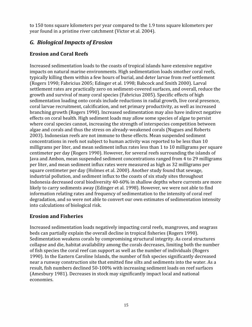
Once length-slope (LS) values for each cell were obtained, cells with a slope greater than 55% were removed from the LS calculation. This was done for two reasons. (1) Steep hillslopes generally have very little soil to erode. The soils that are present are generally being held together by plant roots while most soil production on those sites is slow (Dykes 2002). This means that even if those plants were removed and the soil was eroded, it wouldn’t continue to erode due to the lack of soil production on those sites. (2) The equation we implemented to calculate the slope-steepness factor was calibrated using data from slopes up to 55%, therefore any values calculated for slopes greater than 55% would be extrapolations of the equation (Nearing 1997). The end result of our terrestrial analysis does not significantly change based on what slope we decide to use as a masking point within ±15% of 55% slopes. The results of the combined LS factor can be seen in Figure 6.
Figure 6. Slope and Length-Slope factors

23
Cover Management Factor (C) and Conservation Practice Factor (P)
Literature Review The Cover Management Factor (C) represents the effect of vegetation on soil erosion rates (Renard et al. 1997). It is the ratio of soil loss of a specific crop to the corresponding soil loss under the condition of continuously fallow and tilled land (Renard et al. 1997). The amount of protective coverage provided by the flora influences the soil erosion rate. Continuously fallowed and bare soils have a C value equal to 1. C values are lower when more vegetative coverage protects soils against erosion. Well-protected soils have a C value near 0.
The Conservation Practice Factor (P) represents the impact of a specific conservation practice on soil erosion rates (Renard et al. 1997). It is the ratio of soil loss of a specific practice to the corresponding soil loss caused by up and down slope culture (Renard et al. 1997). The majority of land uses throughout Raja Ampat are non-agricultural and a site visit revealed that only a small fraction of agricultural lands used conservation practices (i.e., terracing, contouring, etc.). Therefore we assume the P value to be 1 throughout the entire region.
Data
Land use data encompassing most of the Raja Ampat region was acquired from CI Indonesia’s field team in Sorong. The original shapefile reflects land use that is current as of 2009, compiled using Landsat imagery and first-person knowledge. Land use for areas that were not included in this dataset, such as Gebe Island, were estimated using 2010 BingMaps Satellite imagery and conversations with locals. For the purposes of this project, some land use types were categorized into similar classifications. Methods
Cover Management Factors (C) have not been determined for the land uses of Raja Ampat using full-scale field tests and rainfall simulator studies. Therefore, C values were estimated based on literature containing comparable land uses from areas with similar geographic and physical processes, consultation with experts, and ground-truthing (Table 3). Assigning C values to corresponding land uses was done by editing the attribute table of the land use shapefile in ArcGIS (Figure 7 and Figure 8). Roads in Raja Ampat ranged in frequency of use, road quality (gravel, grass, limestone, pavement), and width (1-10m). The 90m cell size required for all land use inputs, therefore, drastically overestimates the impacts of roads. To account for this, the C factor for all roads was reduced from 1 to 0.3.

24
Table 3. C Factor literature review
C Factor Source David (1987) Teh (2011) Dumas and
Printemps (2010) Dumas and
Fossey (2009) El-Swaify et al.
(1982) Ridge2Reef
Region Philippines Cameron Highlands, Malaysia
New Caledonia Vanuatu Various locations throughout the
tropics
Raja Ampat, Indonesia
Agriculture 0.38 0.01 0.3
Bare Land 1 1 1 1 1 1
Brush 0.15 0.3 0.72 0.2
Dry Land Forest 0.001-0.003 0.03 0.001 0.001 0.001 0.01
Mangrove 0.01 0.04 0.01
Mining 1 1
Plantation 0.1-0.3 0.1-0.9 0.3
Roads 0.3
Scrubland 0.15 0.25 0.2
Settlement 0.25 0.25
Swamp 0.01 0.28 0

25
Figure 7. Waigeo land use and C factors

26
Figure 8. Batanta (N) and Salawati (S) land use and C factors

27
To demonstrate the utility of the terrestrial model beyond the current land use, we created two example land use scenarios. The conservative land use change scenario models urban growth, agricultural development, and mining activities on slopes primarily less than 20°. The intensive land use change scenario models similar, yet slightly exaggerated development patterns in areas regardless of slope. It is important to note that these scenarios are not meant to predict future land uses in any way, or to provide future development recommendations, but rather to illustrate the utility of the soil erosion model and reveal how various land uses affect soil erosion in different topographic regions. The two example land use scenarios were produced with influence from regional development plans, mineral and heavy metal spatial data, and communication with CI personnel.
Conservative Land Use Change Scenario
Two mines (~230 ha) were placed in northern Waigeo on slopes less than 20°. Most of Gag Island is also mined, however most slopes greater than 20° were avoided. Flat, coastal regions on Waigeo were developed as settlement or agriculture land uses. Throughout much of Raja Ampat, roads were expanded to connect villages by taking a route that results in the least soil erosion. This was done using the Cost Distance and Cost Path tools in ArcGIS 10.1, with values from RUSLE without C factor used as the cost. A 3,700 ha palm oil plantation was placed in western Salawati.
Intensive Land Use Change Scenario
Seven mines (~230 ha) were placed throughout Waigeo in regions thought to contain mineral deposits. Gag Island and Kawe Island are also mined. Urban growth and agricultural development expands slightly beyond what is modeled in the conservative land use change scenario, onto areas with higher slopes. Similar networks of roads are connected between villages without consideration of slopes. Seven 400 ha agricultural plots and a 3,700 ha palm oil plantation were placed on southern Salawati. Rainfall-Runoff Erosivity Factor (R)
Literature Review
The rainfall-runoff erosivity factor (R) represents the erosion potential caused by rainfall. It is defined as the long-term average of the product of total rainfall energy and the maximum 30-min intensity (I30) of rainstorms (Renard et al. 1997; Wischmeier and Smith 1978). Determining I30 requires at least 20 years of pluviograph data, and therefore the calculation of the R-factor may not be possible in many data-poor regions. Numerous methods have therefore been developed to establish a correlation between measured R-values and precipitation data for specific regions. Lo et al. (1985) established an equation based on an empirical study in Hawai’i that uses annual precipitation as an estimator of R-factor for 99 sites (Lee and Heo 2011). The coefficient of determination (R2) was 0.90.

28
Equation 5.
Where:
R – Rainfall erosivity factor (MJ.mm/ha.hr.yr)
P – Mean annual rainfall (mm/yr)
Lo’s equation has since been used by researchers to estimate rainfall erosivity in tropical or subtropical climate regions such as Thailand, Indonesia, and the Philippines (Lee and Heo 2011).
Data
Mean monthly precipitation data (1950-2000) were obtained from WorldClim’s 30 arc-second resolution Bioclim dataset (Hijmans et al. 2005). The raw raster dataset did not entirely cover the region of interest and some pixels had to be extrapolated from surrounding values in ArcGIS. Precipitation in the region varied from 2080-3189 mm yr-1. Methods
Mean monthly precipitation data were used to calculate the rainfall erosivity factor (R) using Lo’s equation. R factors ranged from 766-1155 (Figure 9).
Figure 9. Average annual precipitation (mm) and R factor using (Lo et al. 1985) method

29
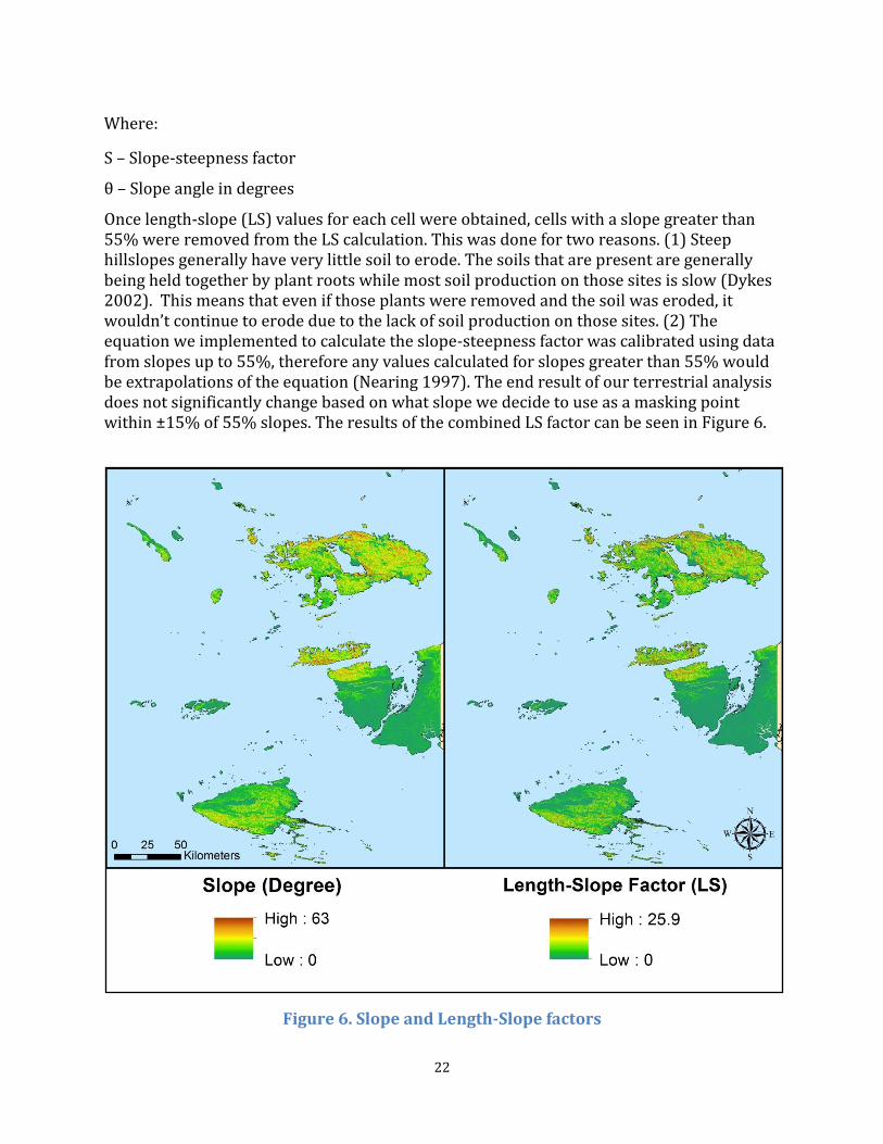
Soil Erodibility Factor (K)
Literature Review
The soil erodibility factor (K) represents an integrated average annual value of the total soil and soil-profile reaction to a large number of erosion and hydrologic processes. These processes include soil detachment and transport by raindrop impact and surface flow, localized deposition due to topography and tillage-induced roughness, and rainwater infiltration into the soil profile (Renard et al. 1997). It is defined as the rate of soil loss per erosivity index unit as measured on a standard plot 22.1m long with a 9% slope, and continuously in a clean-tilled fallow condition, with tillage performed upslope and downslope (Renard et al. 1997).
The most widely used and frequently cited relationship to estimate the K factor is the soil erodibility nomograph (Wischmeier et al. 1971), by using relationships between five soil and soil-profile parameters: percent modified silt (0.002-0.1 mm), percent modified sand (0.1-2 mm), percent organic matter (OM), and classes for structure (s) and permeability (p). Tew (1999) developed a soil erodibility nomograph specific to Malaysia, based on the unmodified soil erodibility nomograph and relative K values obtained from experimental work using a portable rainfall simulator (Figure 10). The equation to calculate K for Malaysian soils is:
Equation 6.
Where:
K – Soil erodibility factor (ton/ha)*(ha.hr/MJ.mm)
M – (% silt + % very fine sand) x (100 - % clay)
OM - % organic matter
s – Soil structure code
p – Permeability code

30
Figure 10. Soil erodibility nomograph (Tew 1999)
Data
Soil data were obtained from the Food and Agricultural Organization of the United Nation’s Harmonized World Soil Database v1.1.
Methods
The dataset included spatially categorized soil types based on similarities in soil characteristics. Each category contained information on percent organic matter, the product of the primary particle size fraction, and the percent of the top four abundant soil types. The soil structure code was derived using a textural classification based on the ratio of clay to sand to silt. The soil permeability codes were based on the soil texture class using the National Soil Handbook (USDA Soil Conservation Staff 1983). K factors were derived using Tew’s (1999) equation (Figure 11).
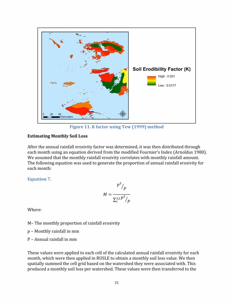
31
Figure 11. K factor using Tew (1999) method
Estimating Monthly Soil Loss After the annual rainfall erosivity factor was determined, it was then distributed through each month using an equation derived from the modified Fournier’s Index (Arnoldus 1980). We assumed that the monthly rainfall erosivity correlates with monthly rainfall amount. The following equation was used to generate the proportion of annual rainfall erosivity for each month: Equation 7.
⁄
∑
⁄
Where:
M– The monthly proportion of rainfall erosivity
– Monthly rainfall in mm
P – Annual rainfall in mm
These values were applied to each cell of the calculated annual rainfall erosivity for each month, which were then applied in RUSLE to obtain a monthly soil loss value. We then spatially summed the cell grid based on the watershed they were associated with. This produced a monthly soil loss per watershed. These values were then transferred to the

32
river mouths for each watershed, resulting in the total amount of sediment exiting each river mouth per month.
B. Marine Model
Overview
Coastal marine dynamics are highly complex, and without the high resolution spatial and temporal data needed to run complex numerical ocean circulation models, many studies have opted to use simpler methods to define the marine areas most likely to be impacted by terrestrial influences (Schill and Raber 2009; Burke and Reytar 2011; Halpern et al. 2008). These methods mainly consist of assigning parameters such as the radius of influence or decay rate that these impacts might have based on expert opinion. These parameters can vary for different impacts such as fishing pressure, terrestrial pollution, sedimentation, etc. Aggregated, they can produce regions of relatively high or low cumulative impact. While these models can serve as rough guides, they do not take into account important oceanographic processes such as current transport, particle settling rates, and water depth, which can drastically change the magnitude and direction of influence.
To better understand where sediment is deposited after entering the ocean, we created a model in Arc GIS 10.1 which uses surface current velocities, settling rates (for each particle size), and bathymetry to produce a potential area of sedimentation. To do this, we first needed to locate the best available information with the greatest spatial coverage of our region. We modeled the year of 2011 for three reasons: (1) the land use data layer was updated to this year, (2) it was a neutral El Niño/La Niña year, and (3) because there was a complete data set across all months for all data layers. For this model we acquired data sets for surface currents, bathymetry, and particle settling rates.
Inputs
Surface Current Data
To determine mean monthly ocean currents in the region we used the hybrid isopycnal-sigma-pressure coordinate ocean model, commonly called HYbrid Coordinate Ocean Model or HYCOM (HYCOM 2013). HYCOM models are isopycnal (constant potential density) in the open, stratified ocean, which is the only regional data that were available to us for this study. The spatial resolution of the data is 1/12° (~9 km). To acquire the HYCOM data we used the Marine Geospatial Ecology Tools (MGET) package developed by Duke University (Duke University 2013), which consists of a free, open-source geoprocessing toolbox for data compilation and downloading. For the purpose of this study we chose to use only the mean monthly east-west and north-south velocity components of the surface currents. This raw data was then processed in ArcGIS 10.1.
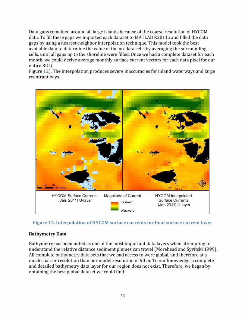
33
Data gaps remained around all large islands because of the coarse resolution of HYCOM data. To fill these gaps we imported each dataset to MATLAB R2011a and filled the data gaps by using a nearest-neighbor interpolation technique. This model took the best available data to determine the value of the no-data cells by averaging the surrounding cells, until all gaps up to the shoreline were filled. Once we had a complete dataset for each month, we could derive average monthly surface current vectors for each data pixel for our entire ROI ( Figure 12). The interpolation produces severe inaccuracies for inland waterways and large reentrant bays.
Figure 12. Interpolation of HYCOM surface currents for final surface current layer
Bathymetry Data
Bathymetry has been noted as one of the most important data layers when attempting to understand the relative distance sediment plumes can travel (Morehead and Syvitski 1999). All complete bathymetry data sets that we had access to were global, and therefore at a much coarser resolution than our model resolution of 90 m. To our knowledge, a complete and detailed bathymetry data layer for our region does not exist. Therefore, we began by obtaining the best global dataset we could find.

34
To do this we turned to the General Bathymetric Chart of the Oceans (GEBCO). GEBCO has multiple global datasets available for download from the British Oceanographic Data Centre (UNESCO 2012). The highest resolution data available, which we acquired, is their global 30 arc-second grids, which translates to a ~900 m pixel (Figure 13). This dataset is an accumulation of multiple data sources including “quality-controlled ship depth soundings with interpolation between sounding points,” “satellite-derived gravity data” and the Shuttle Radar Topography Mission (SRTM) 30m gridded digital elevation models (DEM). The resolution of GEBCOs data vary with location and the amount of available information. GEBCO is then updated as new data sources are identified. Because GEBCO data includes positive values that indicate land, we began by creating a dataset that only accounted for values less than 0. The resulting data covered all of the offshore depths with the best available resolution. However, because of the coarse resolution (~900 m pixel), having the bathymetry meet the shoreline in our region was the exception rather than the rule. Our team acquired a layer of point measurements of ocean depths around our region of interest (Figure 13), which was derived from depth soundings by the Conservation International team over the course of many years. While we could consider this data extremely accurate, it did not cover our entire region of interest and therefore was incomplete for our model. We combined both sources of data by implementing our local depth data where there were gaps between the global GEBCO data. This process consisted of turning both data layers into points and combining them to create a complete bathymetry data set. We then interpolated these points using the Inverse Distance Weighted (IDW) tool in ArcGIS 10.1 at a resolution of 90 m to produce a final bathymetry layer (Figure 14). Finally, because coral reefs typically only extend to depths ≤200 m, we were not concerned with deep-water benthic habitats and other deep-water ecosystem dynamics/services. We therefore excluded all depths greater than 200 m.
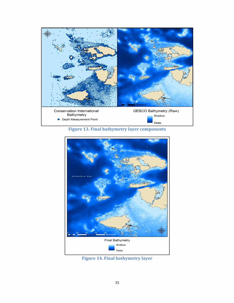
35
Figure 13. Final bathymetry layer components
Figure 14. Final bathymetry layer
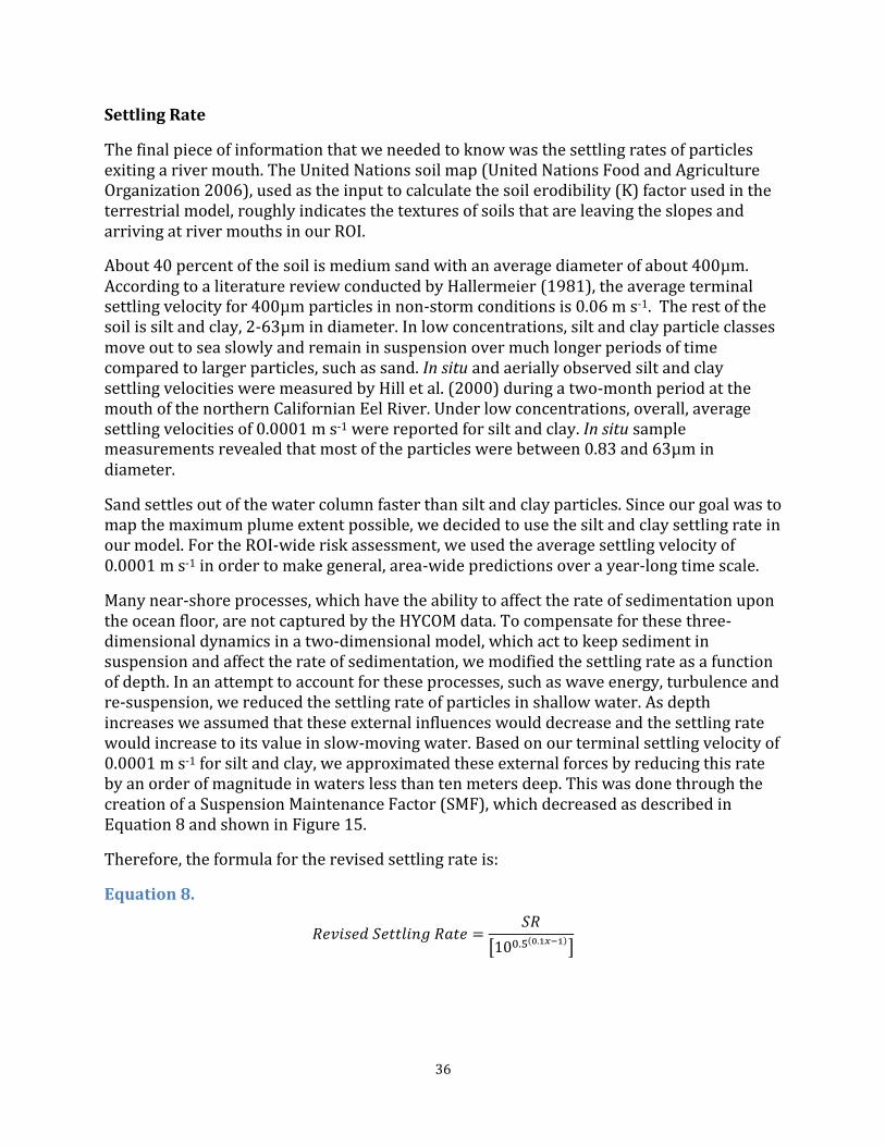
36
Settling Rate
The final piece of information that we needed to know was the settling rates of particles exiting a river mouth. The United Nations soil map (United Nations Food and Agriculture Organization 2006), used as the input to calculate the soil erodibility (K) factor used in the terrestrial model, roughly indicates the textures of soils that are leaving the slopes and arriving at river mouths in our ROI.
About 40 percent of the soil is medium sand with an average diameter of about 400µm. According to a literature review conducted by Hallermeier (1981), the average terminal settling velocity for 400µm particles in non-storm conditions is 0.06 m s-1. The rest of the soil is silt and clay, 2-63µm in diameter. In low concentrations, silt and clay particle classes move out to sea slowly and remain in suspension over much longer periods of time compared to larger particles, such as sand. In situ and aerially observed silt and clay settling velocities were measured by Hill et al. (2000) during a two-month period at the mouth of the northern Californian Eel River. Under low concentrations, overall, average settling velocities of 0.0001 m s-1 were reported for silt and clay. In situ sample measurements revealed that most of the particles were between 0.83 and 63µm in diameter.
Sand settles out of the water column faster than silt and clay particles. Since our goal was to map the maximum plume extent possible, we decided to use the silt and clay settling rate in our model. For the ROI-wide risk assessment, we used the average settling velocity of 0.0001 m s-1 in order to make general, area-wide predictions over a year-long time scale.
Many near-shore processes, which have the ability to affect the rate of sedimentation upon the ocean floor, are not captured by the HYCOM data. To compensate for these three-dimensional dynamics in a two-dimensional model, which act to keep sediment in suspension and affect the rate of sedimentation, we modified the settling rate as a function of depth. In an attempt to account for these processes, such as wave energy, turbulence and re-suspension, we reduced the settling rate of particles in shallow water. As depth increases we assumed that these external influences would decrease and the settling rate would increase to its value in slow-moving water. Based on our terminal settling velocity of 0.0001 m s-1 for silt and clay, we approximated these external forces by reducing this rate by an order of magnitude in waters less than ten meters deep. This was done through the creation of a Suspension Maintenance Factor (SMF), which decreased as described in Equation 8 and shown in Figure 15.
Therefore, the formula for the revised settling rate is:
Equation 8.
[ ]

37
Figure 15. Revised settling rate
We conducted a sensitivity analysis to understand how sensitive the SEM output is to both the SMF and the initial settling rate for still water, the results of which are provided in the Appendix.
We remapped the bathymetry from Figure 14 into 10-meter bins and assigned each bin its respective settling rate. The result was the creation of a new data layer for our entire ROI where every ocean pixel was assigned a specific settling rate based on its associated ocean depth.
Once we had these three pieces of information for the extent of our ROI, we were able to combine them in a model to calculate the maximum distance sediment could travel for each month of 2011. Using surface currents as an input to determine forcing in a particular direction in ArcGIS has been informally discussed in only one study that we could find (Schill 2005), but to our knowledge, this methodology has never formally been published. However, the surface current speed is only an indicator of the vertically averaged current speed throughout the water column.
Path Distance Tool
To first determine how surface currents could affect the lateral movement of sediment we used the “Path Distance” tool in ArcGIS. The path distance tool creates an output raster in which each cell is assigned the accumulative cost from the cheapest source cell while accounting for surface distance and horizontal and vertical cost factors. The algorithm utilizes a node/link cell representation. The cost to travel between one node and the next depends on the spatial orientation of the nodes. How the cells are connected impacts the travel cost as well. Every link has a specific impedance associated with it, which is derived
0.00000
0.00001
0.00002
0.00003
0.00004
0.00005
0.00006
0.00007
0.00008
0.00009
0.00010
0.00011
0 50 100 150 200
Se
ttli
ng
Ra
te (
m/
s)
Depth (m)
Revised Settling Rate as a Function of Depth

38
from the costs associated with the cells at each end of the link (from the cost raster) as well as the direction of movement. This tool requires the following data inputs:
1. Input source data 2. Input cost raster (seconds) 3. Input horizontal raster (degree) 4. Horizontal Factor
Our input source data was the river mouth point locations for our entire ROI (647 points). The input cost raster and the horizontal raster are both derived from our HYCOM surface current data. To create the cost-layer we used Raster Calculator to derive the time in seconds (cost) that it would take to cross an individual cell. To do this we took the width of each pixel (90 m) and divided it by the resulting velocity of the two u (E-W) and v (N-S) vectors (in m s-1):
Equation 9.
√
For the horizontal raster we needed to determine the direction the resulting vector was going across each cell. We did this by taking our u and v velocities and determining an angle of movement. To determine this angle for each pixel we used the following function in Raster Calculator:
Equation 10.
(|
| )
Lastly, the Horizontal Factor (HF) is a user-specified parameter required for the Path Distance tool that defines the relationship between the horizontal cost factor (seconds to cross each cell) and the horizontal relative moving angle (HRMA) (Figure 16). The HF defines the horizontal difficulty encountered when moving from one cell to the next. The HRMA identifies the angle between the horizontal direction of a cell and the moving direction.

39
Figure 16. Horizontal relative moving angle (HRMA) parameter (ESRI 2012)
We had no additional data other than the HYCOM average monthly surface currents, therefore we had no information to tell us that sediment would go anywhere other than “downstream.” To address this, we chose to use the “forward” pre-set parameter setting which establishes that only forward movement is allowed (i.e., down-current) (Figure 17).
Figure 17. Horizontal factor (HF) parameter (ESRI 2012)
Which parameter setting you use to determine the HRMA is extremely important to the scope and direction of the resulting cost layer. After trying various scenarios of each parameter, our team concluded that “forward” was the best selection based on the data availability. The result of this model was an accumulated cost, in seconds to travel towards or away from any river mouth in our ROI while accounting for surface current forcing (Figure 18).

40
Figure 18. Path Distance layer results
Sediment Extent Model
Using the sediment travel time and the particle setting rate, we can determine the depth of any size class of particle at any time. Additionally, each cell has a bathymetry value, so we can determine the distance sediment particles could travel before encountering the ocean floor (Figure 19).
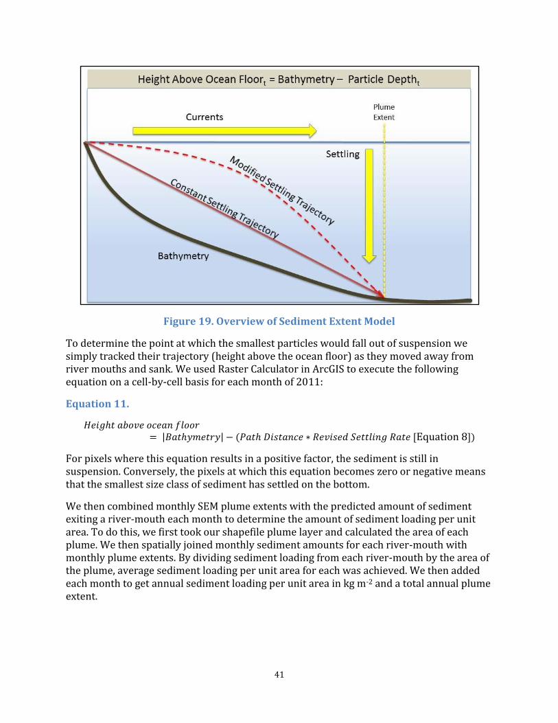
41
Figure 19. Overview of Sediment Extent Model
To determine the point at which the smallest particles would fall out of suspension we simply tracked their trajectory (height above the ocean floor) as they moved away from river mouths and sank. We used Raster Calculator in ArcGIS to execute the following equation on a cell-by-cell basis for each month of 2011:
Equation 11.
| |
For pixels where this equation results in a positive factor, the sediment is still in suspension. Conversely, the pixels at which this equation becomes zero or negative means that the smallest size class of sediment has settled on the bottom.
We then combined monthly SEM plume extents with the predicted amount of sediment exiting a river-mouth each month to determine the amount of sediment loading per unit area. To do this, we first took our shapefile plume layer and calculated the area of each plume. We then spatially joined monthly sediment amounts for each river-mouth with monthly plume extents. By dividing sediment loading from each river-mouth by the area of the plume, average sediment loading per unit area for each was achieved. We then added each month to get annual sediment loading per unit area in kg m-2 and a total annual plume extent.

42
C. Vulnerability Analysis
Data Sources
To determine the areas of marine resources at potential risk from sediment plumes, we used spatial data for the key marine resources of concern:
Coral Reefs
A global dataset provided through ArcGIS 10.1 was used for the location of coral reefs in the region. The dataset represents the global distribution of warm water coral reefs using high-resolution (30 m) satellite imagery from Landsat 7. It was compiled from various data sources that were merged together by United Nations Environment Programme World Conservation Monitoring Center (UNEP-WCMC) and the WorldFish Centre in collaboration with WRI and TNC (UNEP-WCMC 2010). The shapefile was clipped to the Raja Ampat region for use in this analysis.
Marine Protected Areas
The locations of the 12 MPAs within the region were provided by CI in the form of a shapefile.
Dive Sites
The locations of the 147 dive sites within the region were provided by CI in the form of a point shapefile.
Pearl Farms
We created a shapefile for this analysis containing the point locations of the seven pearl farms within the region using information provided by pearl farming companies on their websites. Atlas South Sea Pearl, an Australian pearl farming company, has five farms located in Alyui Bay, Waigeo. Atlas has some 2,500 hectares of water leases capable of supporting over one million adult oysters (Atlas South Sea Pearl Limited 2013). Raja Ampat Mariculture has two farms in the region – one near the town of Bianci in Waigeo, and one near the town of Yenanas in Batanta (Raja Ampat Mariculture LLC 2012).
Analysis
The SEM output raster was converted to a polygon layer to identify the risk zones. We used the Intersect tool within ArcGIS 10.1 to intersect marine resources with these polygons, and then calculated the area or count of each resource within each risk zone. Finally, we calculated the area of the total risk zones over the entire region.

43
V. Results
A. Terrestrial Results
Current Land Use
The predicted rate of annual soil loss in Raja Ampat for the current land use ranged from less than 1 to 702 t ha-1 yr-1 (Figure 20). The values of erosion potential were divided into 5 classes as shown in Table 4. Extreme erosion potential was concentrated in areas where mining has occurred, such as Manuran Island and Gebe Island. High to extreme soil loss rates on Kawe Island, Gag Island, and northern Waigeo are caused mainly by steep slopes and semi-barren scrubland cover. The greater Waisai and Sorong regions also had high to severe erosion potential, due to urban settlement, agriculture, and road development. Kofiau, Misool, Salawati, Batanta, and southern Waigeo generally had low to moderate erosion potential per unit area because of dense forest cover and/or low slopes. Table 4. Ordinal categories of soil erosion potential
Erosion Class Numeric Range (t ha-1 yr-1) Erosion Potential
1 0-5 Low 2 5-10 Moderate 3 10-50 High 4 50-100 Severe 5 >100 Extreme
Annual soil loss at individual river mouths ranged from 8 to 131,000 t yr-1 ( Figure 21). River mouths predicted to release relatively high sediment loads generally drained from larger watersheds. The largest sediment outlets are in northern Waigeo and western Misool, with 89,000 and 131,000 t yr-1 respectively. Other watersheds yielding relatively high amounts of sediment are found on northwestern Waigeo, eastern Mayalibit Bay, Manuran Island, Gebe Island, and the greater Sorong region.

44
Figure 20. Annual sediment loss per hectare under current land use

45
Figure 21. Annual sediment loss per watershed under current land use

46
Conservative Land use Change Scenario The conservative land use change scenario illustrates the potential impact of development in areas where the slopes are primarily less than 20°. The majority of agriculture, urban growth, and road expansion resulted in low to moderate impacts on erosion potential. Some urban growth, specifically near Waisai, had high impacts on erosion potential. Mining is the primary cause for the increase of extreme soil erosion potential between the current and conservative land use change scenarios (Figure 22). The annual soil loss from entire watersheds ranged from 8 to 145,000 t yr-1 (Figure 23). Some small watersheds contributed much higher amounts of total sediment loss under this scenario, due to concentrated development on steep slopes. This is shown on Gag Island and in northern Waigeo, due to mining. The total soil erosion from Gag Island increased from 79,000 t yr-1 to 284,000 t yr-1 between the current and conservative land use change scenarios (Figure 24). Overall, relatively few watersheds had large increases of sediment loss between the current and conservative land use change scenarios (Figure 25).
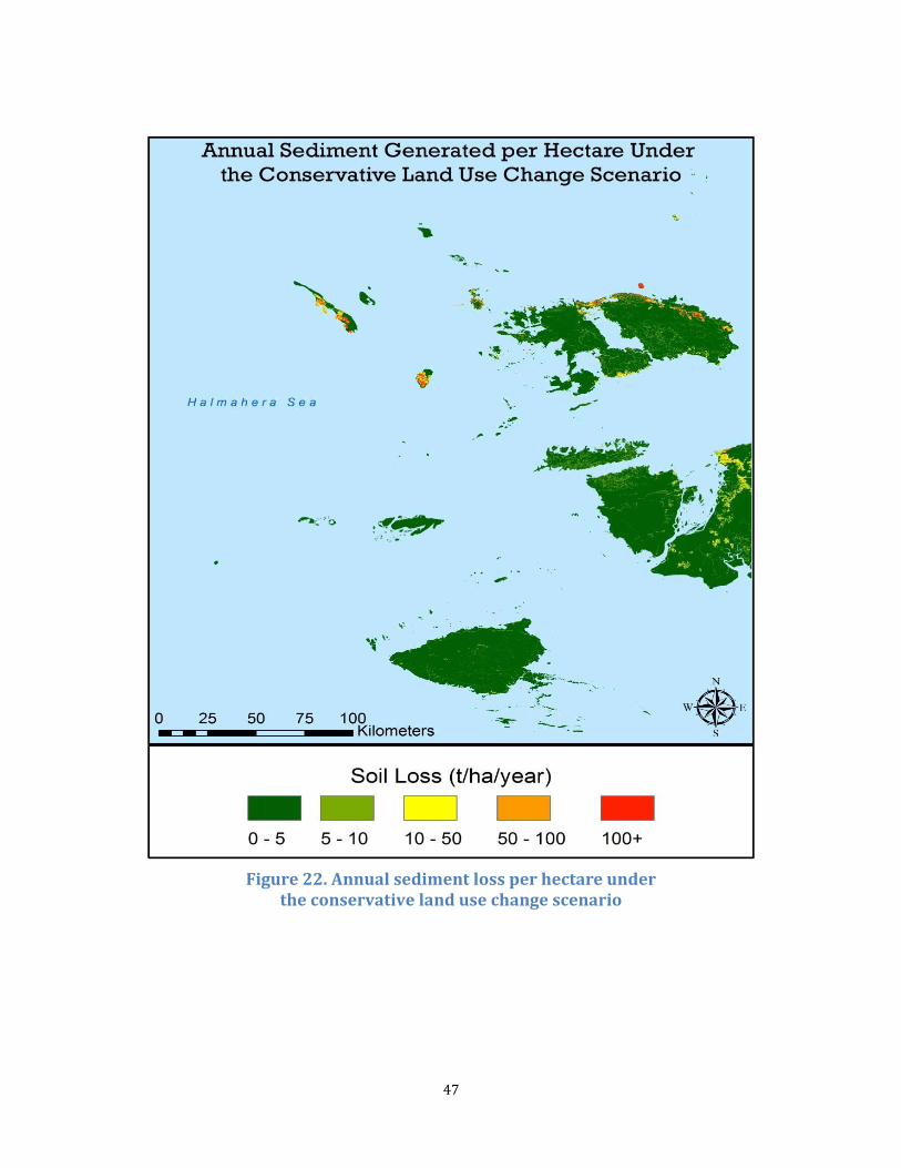
47
Figure 22. Annual sediment loss per hectare under
the conservative land use change scenario

48
Figure 23. Annual sediment loss per watershed under
the conservative land use change scenario

49
Figure 24. Gag Island soil loss rates resulting from mining activities
Figure 25. Difference in annual sediment loss per watershed between
the current and conservative land use change scenario

50
Intensive Land use Change Scenario
The predicted rate of annual soil loss in Raja Ampat for the intensive land use change scenario ranged from less than 1 to 723 t ha-1 yr-1. In this scenario, several mines are placed throughout northern Waigeo, Kawe Island, and Gag Island on slopes greater than 20°, causing extreme soil erosion potential. Other contributing land use changes that resulted in high to extreme erosion rates included urban growth and road development. These types of development were modeled to occur more often on steeper slopes in this scenario, which exacerbated average soil erosion rates for these land uses (Figure 26). The annual soil loss from entire watersheds ranged from 8 to 142,000 t yr-1. Several watersheds yielded 50,000+ t yr-1 under this scenario (Figure 27). However, controlling for acreage and watershed size, the development on Salawati had relatively low impacts on total soil loss by watershed, with increases of ~5,000 t yr-1. Similar to the conservative land use change scenario, concentrated development on steep slopes results in some smaller watersheds yielding much higher amounts of sediment loss under the intensive land use change scenario. The watersheds that show the largest increases in sediment loss surround Mayalibit Bay in Waigeo (Figure 28).

51
Figure 26. Annual sediment loss per hectare under the intensive land use change scenario

52
Figure 27. Annual sediment loss per watershed under
the intensive land use change scenario

53
Figure 28. Difference in annual sediment loss per watershed under
the intensive land use change scenario
The differences in total annual soil loss between the land use scenarios for the entire Raja Ampat region can be seen in Figure 29. The conservative land use change scenario resulted in a 12.7% increase in the total amount of sediment entering the ocean, while the intensive land use change scenario resulted in a 47.1% increase.
Figure 29. Total annual soil loss under each land use scenario
0.00
1.00
2.00
3.00
4.00
Current Conservative IntensiveSo
il L
oss
(m
illi
on
s t
/y
r)
Land Use Scenario
Total Annual Soil Loss in Raja Ampat
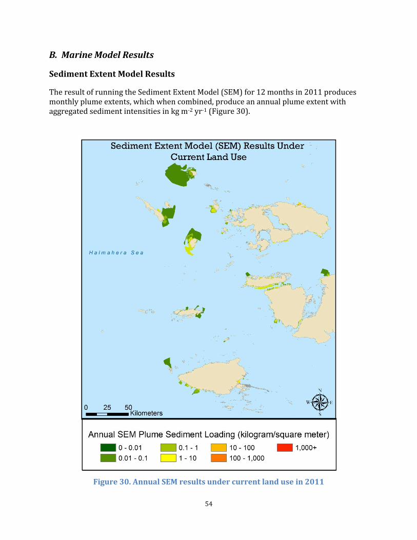
54
B. Marine Model Results
Sediment Extent Model Results
The result of running the Sediment Extent Model (SEM) for 12 months in 2011 produces monthly plume extents, which when combined, produce an annual plume extent with aggregated sediment intensities in kg m-2 yr-1 (Figure 30).
Figure 30. Annual SEM results under current land use in 2011

55
Over the entire Raja Ampat region, our results show that a total of 1,987 km2 of marine habitat were inundated with sediment in 2011 (Table 5). This is over 4% of the total area in our ROI. The largest plume produced by the SEM is in the northeast on Sayang Island, which reaches a maximum extent of 32 km in diameter. This part of the ROI is composed of very deep water with generally strong westward currents. Similarly, Gebe and Gag islands in this area also have large plumes at 19 km and 13 km in diameter respectively. In locations such as Mayalibit Bay and the south coast of Waigeo, generally shallow bathymetry combines with relatively slow moving currents to produce smaller plumes ranging from 2 km to less than 1 km in diameter. Annual and monthly plume extents do not vary between land use scenarios because the size of the plumes are only controlled by surface currents, settling rates, and bathymetry, which stay the same over a standardized time period. However, sediment loading within the plumes does change proportionately with the different land use scenarios. Current Land Use The sediment loading intensity within plumes was derived on a monthly basis to achieve a better understanding of the distribution of sediment both seasonally and annually. Monthly sediment loading was averaged over monthly plume extents. This relationship between plume size and sediment loading produced extremely varied loading intensities between plumes. Regionally, sediment intensity within plumes ranged from nearly 0 to over 1,000 kg m-2 yr-1 (Figure 30). Extremely large sediment intensities were recorded in locations where large amounts of sediment from very large watersheds combined with small marine plume extents. In these types of situations, the model indicates that the sediment exiting a river mouth heads directly into a current that is orthogonal to the coast at that point. The result is that all sediment is trapped at the river mouth. When more detailed current information becomes available this issue will resolve itself. An example location of where this phenomenon occurs and overlaps with marine resources can be seen on Northern Waigeo (Figure 31). Shown in Figure 32, Batanta and northern Salawati both have relatively large plumes with varying degrees of sediment loading. This is due to the variability in monthly plume sizes as well as the monthly variation in sediment loads to the plumes. In this region, there are also multiple marine resources within the plumes. This result demonstrates how this model can be used to identify not only which resources are at risk, but at what level of risk.

56
Figure 31. SEM results on northern Waigeo under current land use
Figure 32. SEM results for Batanta and Salawati under current land use

57
Land use Change Scenarios The results from our conservative land use change scenario can be represented as sediment loading within plume extents as shown in Figure 33. Annual plume sediment loading ranged from nearly 0 to over 1,000 kg m-2 yr-1 with increases in certain plumes reaching upwards of 3000 kg m-2 yr-1. While plume spatial extents do not change, sediment loading within those plume extents does change. As one would expect, sediment loading within plumes changes proportionally to the change in terrestrial soil loss. This result could again be looked at on a monthly basis to understand the relationship between sediment loading and both plume direction and area. The information gained by a monthly analysis could be used to better inform stakeholders of particularly impactful months and/or seasons.
Figure 33. SEM results under the conservative land use change scenario

58
Under our intensive land use change scenario, annual plume sediment loading increased proportionally to that of the terrestrial model. These changes are not readily apparent at
the ROI scale, and therefore these small changes in annual plume sediment loading can be better visualized at the fine scale.
Figure 34 shows a comparison of the annual SEM plume sediment loading across all three land use scenarios for Gag Island and in the area surrounding the city of Waisai, located on southern Waigeo. On Gag Island, increases in sediment loading are mainly due to mining under both the conservative and intensive land use change scenarios. We can see increasing intensity of plumes on the western side of Gag Island, particularly under the intensive land use change scenario. Increases in sediment loading around Waisai are mainly due to increases in settlement and agriculture, as well as some road development, under both the conservative and intensive land use change scenarios. Particularly under the intensive land use change scenario, we can see increasing intensity of plumes on the southeastern edge of the coastline shown in the map of Waisai. A comparison of the annual SEM plume sediment loading across all three land use scenarios for Batanta is shown in Figure 35. Increases in sediment loading are mainly due to road development on this island under both the conservative and intensive land use change scenarios. Areas on both the northern and southern coasts of Batanta show increasing intensity of plumes, particularly under the intensive land use change scenario. In combination, the results of these three different land use scenarios visually communicate the spatial extent and degree of influence various land use change scenarios may have on marine resources.

59
Figure 34. SEM results under all land use scenarios for Gag Island and Waisai on southern Waigeo

60
Figure 35. SEM results under all land use scenarios for Batanta

61
Vulnerability Analysis Results
Once we produced the SEM output, we overlaid these plumes with marine resources to calculate the area of overlap (Table 5). Within the identified plume extents we found 57 km2of coral reefs, 479 km2 of MPAs, 4 dive sites and 1 pearl farm. The total 2011 plume extents encompass an area of 1,987 km2. Finally we identified other benthic habitats at risk. These represent habitats within the risk zones that are not coral reefs. These areas totaled 1,930 km2. Table 5. Marine resources within 2011 SEM plume extents
Total Area or Count
Coral Reefs 57 km2
MPAs 479 km2
Dive Sites 4
Pearl Farms 1
Other Benthic Habitats 1,930 km2
Plume Extents 1,987 km2
ROI 43,000 km2
VI. Discussion We developed a novel tool that links sediment loss on land to spatial predictions of its extent and intensity in the ocean as a function of surface currents, bathymetry, and a modified settling rate. Our analysis demonstrated the utility of this tool in two main ways.
A. Terrestrial Model
The terrestrial model predicts soil loss from land using a RUSLE calibrated for steep, tropical island regions for a range of user-defined land use scenarios. The model predicted soil erosion ranging from less than 1-723 t ha-1 yr-1, which is comparable with other studies modeling soil erosion (Anghel and Todică 2008; Sujaul et al. 2012; Pimentel and Kounang 1998; Teh 2011). Forest and agriculture are thought to yield soil losses at a rate of 0.001-5 and 13-40 t ha-1 yr-1, respectively (Pimentel and Kounang 1998). To demonstrate the utility of this tool to planners interested in understanding the influence of land use change on soil erosion, two additional scenarios reflecting conservative and intensive land use change were modeled. These scenarios are not presented as a prediction of expected development, but rather to illustrate how changes in C factors will impact the amount of soil erosion predicted by the model. The upper range of soil erosion rates between land use scenarios did not vary much (702 – 723 t ha-1 yr-1) as they are the result mining activities; however, the distribution of soil erosion rates changed considerably. The average rate of soil erosion per hectare increased between current, conservative, and intensive land use change scenarios for nearly all land use classes, which is generally due to

62
land use changes occurring on steeper slopes (Table 6). This illustrates the influence that land use and slopes have on changes in soil erosion rates. Table 6. Average soil erosion rates for land use classes between land use scenarios
Average Soil Erosion Rates (t ha-1 yr-1)
Current Conservative Δ% from Current
Intensive Δ% from Current
Dry Land Forest 1.3 1.3 0 1.3 0
Agriculture 12.1 9.2 -24 9.9 -18.2
Settlement 10.6 9.4 -11.3 14.5 36.8
Roads 15.5 16.8 8.4 29.1 87.7
Mines 56.6 63.6 12.4 88.9 57.1
It follows that as the average soil erosion rates per hectare increase with intensified development, the total sediment yields from watersheds to river mouths also increase. Table 7 shows that the number of watersheds with relatively large sediment yields (>10,000 t yr-1) increased 15% and 35% from the current land use scenario to the conservative and intensive land use change scenarios, respectively. Table 7. Watersheds losing high amounts of soil between land use scenarios
Watersheds yielding > 10,000 t yr-1
Current Conservative Intensive
Number of watersheds 60 69 81
Δ% -- 15 35
By removing the C factor from the RUSLE model, watersheds can be identified that are more sensitive to the influence of land use on increases in soil erosion. Figure 36 shows that Batanta, the northern coast of Salawati, Kawe Island, and Waigeo are particularly sensitive. Development to these areas is therefore likely to result in large increases in soil erosion relative to other regions. By identifying patterns of different erosion rates caused by land use changes, more informed management decisions could be made when planning for development. However, some limitations and levels of uncertainty in our predictions exist.
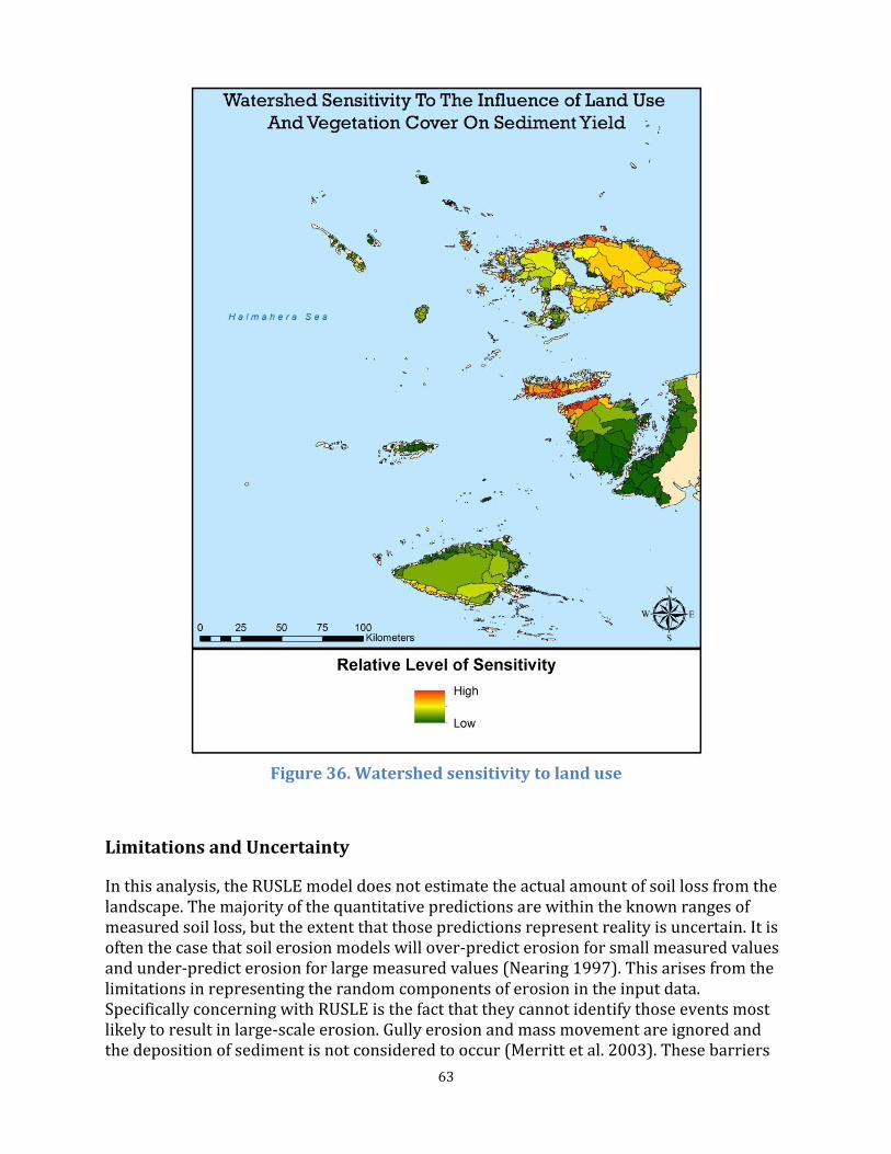
63
Figure 36. Watershed sensitivity to land use
Limitations and Uncertainty
In this analysis, the RUSLE model does not estimate the actual amount of soil loss from the landscape. The majority of the quantitative predictions are within the known ranges of measured soil loss, but the extent that those predictions represent reality is uncertain. It is often the case that soil erosion models will over-predict erosion for small measured values and under-predict erosion for large measured values (Nearing 1997). This arises from the limitations in representing the random components of erosion in the input data. Specifically concerning with RUSLE is the fact that they cannot identify those events most likely to result in large-scale erosion. Gully erosion and mass movement are ignored and the deposition of sediment is not considered to occur (Merritt et al. 2003). These barriers

64
arise due to a combination of natural complexity, spatial heterogeneity, and the lack of available data (De Vente and Poesen 2005). Soil erosion fluctuates over space and time due to multiple processes, their interactions, and the temporal and spatial variability of those processes. Many of these influencing processes are complex and are difficult to include in soil erosion modeling. This often leads to processes being ignored or simplified, as is the case with our terrestrial model (Wang et al. 2002). RUSLE instead relies on empirical regression to define factors which influence soil erosion. Simplifying these processes into factors introduces uncertainty in estimates of soil erosion. Uncertainty can also arise from the spatial and temporal properties of data inputs into the model. In addition the interactions of RUSLE factors are not well represented in their calculation, leading to further uncertainty (Renard et al. 1997). The rainfall erosivity factor used in this analysis introduces uncertainty in several ways. First, the precipitation data used to calculate the rainfall erosivity factor was in the form of interpolated average monthly precipitation from approximately 1950 to 2000, which was compiled into average annual precipitation. This dataset is worldwide, and the confidence of the values produced by interpolation is directly affected by the number of rain gauge stations in a given area. Data for this region was interpolated using a limited number of stations. While the general patterns of precipitation are represented, the accuracy of those values at specific locations is in question. Second, to calculate the values for the rainfall erosivity factor we aggregated monthly precipitation over the year. This temporal lumping ignores two important components of soil erosion, rainfall energy and rainfall intensity. Rainfall intensity is the rate of precipitation and acts as the soil particle detachment mechanism. Rainfall energy indicates the transport capacity of precipitation. Rainfall events with higher rainfall intensity will tend to cause more soil loss than events with lower intensity but more rainfall energy (Renard et al. 1997). These factors are functions of the individual rainstorms that produce them, which are not incorporated into this analysis. The soil erodibility factor introduces uncertainty into this analysis through spatial and temporal variability. The soils data utilized for this analysis was derived from a global dataset, which generalizes the soil types in Raja Ampat to only a few categories. Soils vary through a landscape with much more complexity than is represented in this dataset. Furthermore, over time soil properties can be altered by plants, climate, and through human activities such as agriculture (Wang et al. 2001). While the cover management factor was based on a classification rather than an equation, uncertainty still exists for several reasons. Values from studies elsewhere were applied to similar land uses in Raja Ampat (Table 3). It was often the case that the literature could not provide a cover factor that exactly matched a land use in the region, requiring judgment in deciding what the cover factor should be. Lastly, there were limitations with small areas of a particular land cover types such as roads and the 90m pixel size used in this analysis. The cover factor values of these land cover types were therefore reduced to compensate for the discrepancy between the resolution of our data and the real size of these features on the landscape. The length-slope factor is often cited as the most influential and troublesome factor when applying any version of the USLE to complex topography (Zhang et al. 2013). Issues arise

65
regarding how to define both the slope length and the effect of slope steepness in heterogeneous topography. For this analysis, the slope length was defined as 90m, the pixel size of the DEM. This is a gross over-simplification, and undoubtedly produced uncertainty in the results. However, due to issues that arise with soil loss modeling at large scales, setting the slope length to 90 meters was the best option. Another source of uncertainty was the length-slope factor’s inability to capture spatial topographical variability. The effects of concave and convex slopes are not well represented in this calculation of the length-slope factor. In addition to the uncertainty associated with estimating RUSLE factors, the terrestrial model fails to address several elements. First, the soil erosion rates associated with mining are probably lower than this model predicts because of management practices that likely require at least some mine tailings to be disposed of properly. Second, the model fails to address the impacts of logging. Logging has limited legal status in most regions of Raja Ampat, and is often selective rather than clear-cut. The contribution of this type of logging to soil erosion is still significant; however, accurately modeling this type of land use change at a 90 m scale is not possible. Additionally, the spatial data corresponding to selective logging activities is extremely difficult to obtain. Third, the qualities of roads vary from 1m wide trails covered by grass and surrounded by lush vegetation to 10 m wide paths of loose soil cut through landscapes that leave steep banks of exposed soil. The soil loss rates from roads modeled in this analysis are therefore likely a combination of under and overestimates. Finally, the watershed delineation required a minimum size threshold, excluding most of the coastal areas from the model. Since the vast majority of island development occurs within a short distance to coast, a significant amount of soil erosion may be missing from this analysis. In summary, the purpose of the terrestrial modeling was to obtain a general sense of how much sediment is being generated within drainage basins and where it was leaving the terrestrial landscape. The purpose of this approach was use the analysis as a planning tool to demonstrate how varying land uses could affect sedimentation rates and annual sediment yields being delivered to river mouths. This approach avoids the need for precise sedimentation modeling, allowing users to obtain an overall picture of what areas could be of concern and what areas could endure land use change while minimally impacting sedimentation rates. The team used the best available data for the region to define the inputs to the terrestrial model. Local data collections and in situ calibrations of equations will greatly reduce the level of uncertainty and increase the accuracy of model predictions.
B. Marine Sediment Extent Model
The second component of the tool, the marine Sediment Extent Model (SEM) uses surface currents, bathymetry, and a modified settling rate to predict the maximum extent of sediment deposition from each river mouth over a specified time period. Broadly, the output shows monthly sediment “plume” extent with monthly terrestrial model-generated sediment loads averaged per unit area, which are then aggregated to achieve an annual plume extent and sediment distribution. These plumes extend out from each river mouth in a color-coded scale that shows relative amounts of sediment within the plumes (Figure 30). Input data sets are available globally and for different temporal scales, which provides flexibility in using the model in other locations and for various time scales and periods. For

66
this analysis, we used monthly data over a year-long period. However, HYCOM current data is available in more fine temporal increments, making increases in temporal resolution possible. While the SEM does not predict the distributional patterns of sediment within the plume extents, it can determine the contribution of sediment loads within discrete time periods to the aggregated plume over a larger time scale. This allows users to identify hotspots of risk within the overall area of possible sediment impact. This analysis demonstrates this utility by mapping monthly sediment loads averaged over each respective monthly plume extent to get sediment loading per area (kg m-2 month-1). These monthly plumes (see examples in Figure 37 and Figure 38) are then aggregated to produce a maximum annual sediment extent.
Figure 37. SEM results for Batanta and Salawati under
current land use (shown for the month of February)
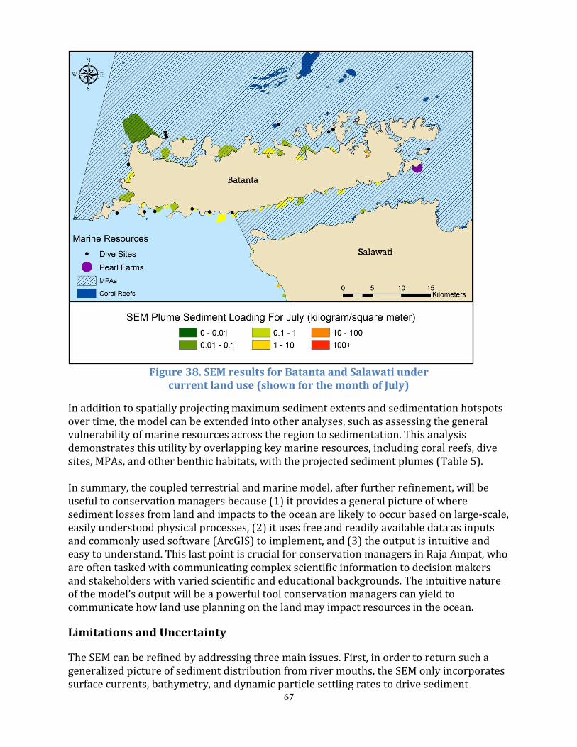
67
Figure 38. SEM results for Batanta and Salawati under
current land use (shown for the month of July)
In addition to spatially projecting maximum sediment extents and sedimentation hotspots over time, the model can be extended into other analyses, such as assessing the general vulnerability of marine resources across the region to sedimentation. This analysis demonstrates this utility by overlapping key marine resources, including coral reefs, dive sites, MPAs, and other benthic habitats, with the projected sediment plumes (Table 5). In summary, the coupled terrestrial and marine model, after further refinement, will be useful to conservation managers because (1) it provides a general picture of where sediment losses from land and impacts to the ocean are likely to occur based on large-scale, easily understood physical processes, (2) it uses free and readily available data as inputs and commonly used software (ArcGIS) to implement, and (3) the output is intuitive and easy to understand. This last point is crucial for conservation managers in Raja Ampat, who are often tasked with communicating complex scientific information to decision makers and stakeholders with varied scientific and educational backgrounds. The intuitive nature of the model’s output will be a powerful tool conservation managers can yield to communicate how land use planning on the land may impact resources in the ocean.
Limitations and Uncertainty
The SEM can be refined by addressing three main issues. First, in order to return such a generalized picture of sediment distribution from river mouths, the SEM only incorporates surface currents, bathymetry, and dynamic particle settling rates to drive sediment
68
movement and deposition in the ocean. However, other processes besides average monthly regional current velocity affect sediment transport. For example, several studies have cited tides as the dominant near-shore process controlling sediment dispersal out of river mouths (Curran et al. 2007; Nowacki and Ogston 2012). While the SEM does not specifically take tides into account, average monthly HYCOM currents do incorporate tides; however, the effects of local tidal fluctuations in the context of coastal geography are not captured in the low resolution of the current data. Likewise, because this is a two-dimensional model, three-dimensional dynamics such as vertical mixing, freshwater forcing, bottom friction and re-suspension are not being represented. All of these factors could potentially increase or decrease the extent of plumes and thus sediment intensity within the plumes. In order to compensate for these latter processes, the team modified the settling rate to decrease with decreasing depth. However, future in situ measurements and regional calibration of the true settling rates will help fine-tune the suspension maintenance factor to more accurately reflect how sediment is dispersed in the near-shore marine environment. Second, the SEM can also be improved with better near-shore current data. There were large gaps between the best surface current data available, the u and v products of the HYCOM model, and the shoreline of the islands. Due to the requirements of the SEM, the currents data therefore had to be interpolated up to the shoreline using a nearest-neighbor averaging algorithm ( Figure 12). While a detailed assessment of near-shore current velocities might predict vastly different fine-scale values, this method depicts broad-scale direction and magnitude of current velocity. The model could be improved, for example, by asking local boat users to keep an hourly log of GPS-registered current directions throughout each work day. The low resolution of both the bathymetry and the surface currents is also the reasoning for the “blocky” look to the plumes, which is not characteristic of actual sediment plumes. Third, the model currently does not have a way to change the direction of currents that are perpendicular to the shoreline. In many places, the HYCOM data contained an average resultant current vector pointing towards the land. The result is that SEM predictions do not allow sediment from a river mouth at such places to migrate along or away from the shoreline. Deposition occurs at the river mouth and the sedimentation per unit area is counter-intuitively high there. In the real environment, the magnitude and direction of these velocity vectors would become less orthogonal as they approached land, resulting in long-shore transport. Therefore, if the HYCOM currents are near the shore and pointing towards a river mouth, sediment simply remains in the cells nearest the source river mouth because there is no mechanism in place by which it may escape. One way this issue could be resolved without enhancing the model’s current capability would be to use high-resolution current data. However, this analysis could be costly and time consuming. An alternate approach could include further processing of the HYCOM current input to both interpolate and redirect currents as they approach the shoreline. Because bathymetry and coastal alignment are the primary influences on the direction of water movement in the near-shore region, this next step would alleviate the need for better data and vastly improve the modeling capabilities. This hypothetical model would initially check the relative angle of the currents within some distance of the coastline. It would then re-evaluate current direction to follow a gradual transition towards long-shore transport.

69
Similar to the terrestrial model, the SEM plume estimates can be improved with better data. In situ measurements and regional calibration efforts can be extended to model calibration and validation. Due to its remote location and high degree of cloud cover, Raja Ampat is a satellite data-poor region. We did not find cloud-free aerial or satellite imagery with which to compare the SEM predictions to real plumes for validation purposes. The rain gauge data on Raja Ampat available to us is limited in several ways. The data are limited to one location in the region, the city of Sorong, located on the west coast of West Papua, the data were collected over a short time period (1994-2010), and the data were reported as monthly averages. This data could therefore not be used to identify when specific storm events occurred to guide satellite imagery searches for those scenes that spatially and temporally corresponded to storm events, which could likely show the maximum plume extents. The maximum distance sediment plumes predicted by the SEM extend agree with many previously published observed sediment plume extents (Warrick et al. 2004; Kineke et al. 2000; Renagi et al. 2010; Morehead and Syvitski 1999; Nowacki et al. 2012). However, most of the reviewed sediment plume modeling literature couples modeling efforts with measurements (Warrick et al. 2004; Kineke et al. 2000; Renagi et al. 2010; Morehead and Syvitski 1999; Nowacki et al. 2012), but because of time and funding constraints we were unable to do the same.
C. Vulnerability Analysis
To demonstrate the extended utility of the tool, we also conducted a vulnerability analysis to quantify the total area of marine resources that are likely to be impacted by sediment from river mouths. The output of the SEM produces an average annual approximation of plume extent for river mouths. We used the overlap between these plumes and key marine resources to calculate the at-risk areas. The SEM model shows that 57 km2 of coral reefs, 4 dive sites, 1 pearl farm, and 479 km2 of MPAs should have received some sediment in 2011 (Table 5). The total area of MPAs affected by the risk of sediment extent is greater than the total area of coral reefs affected, but the MPAs cover a larger area of the region and therefore have a smaller percentage at risk from sediment extent. Many of the dive sites that were not directly overlapped by the sediment extent plumes were close to predicted sedimentation zones, suggesting that they might be affected during more intense current regimes in some years, especially if the model performance is enhanced with higher-resolution current data. Very little information is available on the location and size of pearl farms throughout Raja Ampat. It is unknown whether or not there are additional farms in the area that were not included in the database available to us, and the spatial extent of the pearl farms included in this study was not recorded. Definition of their extent would lead to improvement in the calculation of impact. The area of all plumes totaled 1,987 km2, which covers about 4.6% of the total area of the Raja Ampat region. Additionally, our database only contains known and frequently visited coral reefs and dive sites. Because this model is restricted to seabed within the photic zone (depths shallower than -200 m), we can assume that high levels of productivity at all trophic levels will be found throughout the majority of this area. With improved marine resource spatial data, the overlap analysis of the SEM model with our marine resource

70
spatial data grossly underestimates the true amount of coral reefs, MPAs, and dive sites and other marine resources that are vulnerable to sedimentation.
VII. Conclusions
A. The Model as a Framework We developed a coupled terrestrial and marine model to assess how land use changes impact the amount of sediment entering the ocean and determine where that sediment is dispersed. This tool made it possible to assess the vulnerability of the region’s marine resources to increases in sedimentation to be expected from hypothetical land use change scenarios, thereby specifically addressing the needs of CI. The tool is flexible in terms of spatial and temporal extent and can be applied to a variety of other planning processes. Our tool can be refined with improved local data, including more accurate land cover (and predicted land use change), as well as fine-scale near-shore currents. In addition, the tool is adaptable to seasonality considerations for erosion and currents. The tool could be used to focus on sedimentation during rainy months or during periods of the year when currents have the potential to carry sediment further out into the ocean. This tool is an important first step in helping visualize the linked effects of land erosion and ocean impacts, but there is still work to be done. There are two main ways to improve the model’s functionality. The most influential improvement would be to get high resolution current data in the near-shore environment that accurately represents long-shore current movement. Another way would be to alter interpolated HYCOM or other coarse-scale data so that it approximates this effect within the modeling environment. The tool would be most useful to land use planning efforts after these issues are addressed.
B. Suggestions for Further Research In doing our analysis, we identified several possible applications of the tool we developed, including taking the tool from the coarse-grained assessment we did and narrowing to a more fine-scale analysis of key areas of concern for future land use change. The tool could be used on a watershed-by-watershed basis to provide a higher resolution environmental impact assessment. Beyond sedimentation modeling, research focusing on the biological and economic impacts of sedimentation on Raja Ampat will be an important complement to this tool when making complex land use planning decisions. Marine resources at risk could expand beyond our identified risk zones because of ecological factors such as connectivity and interdependence of marine environments. Negative impacts to a coral reef from sedimentation will likely influence the ecosystem function of adjacent reefs and the species that depend on them over time. Therefore, it would be useful to do further research on the linkages between sedimentation and the biological impacts on key marine resources. In addition, a quantitative link between quantities and intensities of sedimentation on coral reefs and coral reef health and mortality is not known. Research efforts to make this link will be invaluable for refining estimates of risk to coral reefs from sedimentation due to land use change. Furthermore, better understanding the degree to which sedimentation degrades coral reefs could help

71
quantify the monetary value lost when reefs are degraded. This information could make cost-benefit analyses relating to planning decisions better represent reality. Finally, conducting an economic analysis to evaluate the costs and benefits of various development and land use options would help provide a different picture of the impacts of sedimentation on marine resources. Our analysis highlighted several watersheds that pose a high risk of increased sedimentation due to land use change. Additionally, we now have a generalized understanding of where the risk of sediment transport overlaps with important marine resources, connecting actions on land to consequences in the ocean. On a purely physical science base, we could recommend foregoing development within specific watersheds in order to preserve the integrity and long term sustainability of the marine environment. However, land use planning is shaped by stakeholder demands other than those of the conservation community, and the Regency of Raja Ampat will no doubt wish to explore options that balance conservation with the economic development of its communities. Economic data is available on sectors important to the Raja Ampat Regency, but lacking at any finer scale. We recommend a rigorous economic analysis to evaluate the costs and benefits of various development and land use options that could be adopted by Regency leadership. In particular, a quantitative connection between risk of sedimentation to marine resources and sector profitability must be made to ensure well-informed decision making endeavors.
72
References Agostini, V.N., H.S. Grantham, J. Wilson, S. Mangubhai, C. Rotinsulu, N. Hidayat, A. Muljadi, M.
Mongdong, A. Darmawan, L. Rumetna, M.V. Erdmann, and H.P. Possingham. 2012. Achieving Fisheries and Conservation Objectives within Marine Protected Areas: Zoning the Raja Ampat Network.
Amesbury, S.S. 1981. Effects of Turbidity on Shallow-water Reef Fish Assemblages in Truk, Eastern Caroline Islands. In Proceedings of the Fourth International Coral Reef Symposium 1: 155–159. Manilla.
Anghel, T., and S. Todică. 2008. Quantitative Assessment of Soil Erosion Using GIS Empirical Methods - A Comparative Study between the Motru Mining Area and the Suceviţa Catchment. Annals of the University of Oradea - Geography Series (5): 95–102.
Arnoldus, H.M.J. 1980. An Approximation of the Rainfall Factor in the Universal Soil Loss Equation. Food and Agriculture Organization.
Atlas South Sea Pearl Limited. 2013. “Our Pearl Farms.” http://www.atlassouthseapearl.com.au/advantages/our-pearl-farms.
Baban, S.M.J. 1995. The Use of Landsat Imagery to Map Fluvial Sediment Discharge into Coastal Waters. Marine Geology 123 (April): 263–270. http://linkinghub.elsevier.com/retrieve/pii/002532279500003H.
Babcock, R., and L. Smith. 2000. Effects of Sedimentation on Coral Settlement and Survivorship. In 9th International Coral Reef Symposium, 23–27. Bali, Indonesia.
Bailey, M., and T. Pitcher. 2008. Ecological and Economic Analyses of Marine Ecosystems in The Bird’s Head Seascape, Papua, Indonesia: II. Fisheries Centre Research Reports. Vol. 16.
Burke, L., and K. Reytar. 2011. Reefs at Risk Revisited: Technical Notes on Modeling Threats to the World’s Coral Reefs.
Cesar, H.J.S. 2002. Coral Reefs : Their Functions, Threats and Economic Value. In I. (Cesar, H.J.S., Ed.) CORDIO, Department for Biology and Environmental Sciences, Kalmar University, Kalmar, Sweden: 14–39.
Consultative Group on International Agricultural Research – Consortium for Spatial Information (CGIAR-CSI). 2013. “SRTM 90m Digital Elevation Database V4.1.” http://www.cgiar-csi.org/data/srtm-90m-digital-elevation-database-v4-1.
Choi, J.-K., Y.J. Park, J.H. Ahn, H.-S. Lim, J. Eom, and J.-H. Ryu. 2012. GOCI, the World’s First Geostationary Ocean Color Observation Satellite, for the Monitoring of Temporal Variability in Coastal Water Turbidity. Journal of Geophysical Research 117 (September 1). http://www.agu.org/pubs/crossref/2012/2012JC008046.shtml.
Curran, K.J., P.S. Hill, T.G. Milligan, O.A. Mikkelsen, B.A. Law, X.D. de Madron, and F. Bourrin. 2007. Settling Velocity, Effective Density, and Mass Composition of Suspended Sediment in a Coastal Bottom Boundary Layer, Gulf of Lions, France. Continental Shelf Research 27 (June): 1408-1421. http://linkinghub.elsevier.com/retrieve/pii/S0278434307000441.

73
Curran, K.J., P.S. Hill, and T.G. Milligan. 2002. Fine-grained Suspended Sediment Dynamics in the Eel River Flood Plume. Continental Shelf Research 22 (November): 2537–2550. http://linkinghub.elsevier.com/retrieve/pii/S0278434302001292.
David, W. 1987. Erosion and Sediment Transport. Upland Resource Policy Program. Philippine Institute for Development Studies (PIDS) Working Paper 87-01. Makati: PIDS.
Dive Raja Ampat. 2010. “Conserving Raja Ampat.” Dive Raja Ampat. http://diverajaampat.org/info/Conserving/conserving.html.
Donnelly, R., D. Neville, and P.J. Mous. 2002. Report on a Rapid Ecological Assessment of the Raja Ampat Islands, Papua, Eastern Indonesia. October.
Duke University. 2013. “Marine Geospatial Ecology Tools (MGET).” http://mgel.env.duke.edu/mget.
Dumas, P., and M. Fossey. 2009. Mapping Potential Soil Erosion in the Pacific Islands: A Case Study of Efate Island (Vanuatu). In 11th Pacific Science Inter-Congress: Pacific Countries and Their Ocean, Facing Local and Global Changes.
Dumas, P., and J. Printemps. 2010. Assessment of Soil Erosion using USLE Model and GIS for Integrated Watershed and Coastal Zone. In Proceedings Interpraevent 2010, International Symposium in Pacific Rim, 856–866.
Dykes, A.P. 2002. Weathering-limited Rainfall-triggered Shallow Mass Movements in Undisturbed Steepland Tropical Rainforest. Geomorphology 46 (July): 73–93. http://linkinghub.elsevier.com/retrieve/pii/S0169555X02000557.
Ebisemiju, F.S. 1990. Sediment Delivery Ratio Prediction Equations for Short Catchment Slopes in a Humid Tropical Environment. Journal of Hydrology 114: 191–208.
Edinger, E.N., J. Jompa, G.V. Limmon, W. Widjatmoko, and M.J. Risk. 1998. Reef Degradation and Coral Biodiversity in Indonesia: Effects of Land-based Pollution, Destructive Fishing Practices and Changes over Time. Marine Pollution Bulletin 36 (8): 617–630.
El-Swaify, S.A., E.W. Dangler, and C. L. Armstrong. 1982. Soil Erosion by Water in the Tropics. University of Hawaii: Honolulu, Hawaii.
Erdmann, M.V., and J.S. Pet. 2002. A Rapid Marine Survey of the Northern Raja Ampat Islands. Henry Foundation/The Nature Conservancy/NRM/EPIQ June 2002.
ESRI. 2012. “ArcGIS 10.1 Help Resources: How the Path Distance Tools Work.” http://www.esri.com.
Fabricius, K.E. 2005. Effects of Terrestrial Runoff on the Ecology of Corals and Coral Reefs: Review and Synthesis. Marine Pollution Bulletin 50 (February): 125–46. http://www.ncbi.nlm.nih.gov/pubmed/15737355.
Golbuu, Y., S. Victor, E. Wolanski, and R.H. Richmond. 2003. Trapping of Fine Sediment in a Semi-enclosed Bay, Palau, Micronesia. Estuarine, Coastal and Shelf Science 57 (August): http://linkinghub.elsevier.com/retrieve/pii/S0272771402004249.
Hallermeier, R. 1981. Terminal Settling Velocity of Commonly Occurring Sand Grains. Sedimentology 28: 859–865.
74
Halpern, B.S., S. Walbridge, K.A. Selkoe, C.V. Kappel, F. Micheli, C. D’Agrosa, J.F. Bruno, K.S. Casey, C. Ebert, H.E. Fox, R. Fujita, D. Heinemann, H.S. Lenihan, E.M.P. Madin, M.T. Perry, E.R. Selig, M. Spalding, R. Steneck, and R. Watson. 2008. A Global Map of Human Impact on Marine Ecosystems. Science 319 (February 15): 948–952. http://www.ncbi.nlm.nih.gov/pubmed/18276889.
Hijmans, R.J., S.E. Cameron, J.L. Parra, P.G. Jones, and A. Jarvis. 2005. Very High Resolution Interpolated Climate Surfaces for Global Land Areas. International Journal of Climatology 25: 1965–1978.
Hill, P.S., T.G. Milligan, and W.R. Geyer. 2000. Controls on Effective Settling Velocity of Suspended Sediment in the Eel River Flood Plume. Continental Shelf Research 20 (December): 2095–2111. http://linkinghub.elsevier.com/retrieve/pii/S0278434300000649.
Holmes, K.E., E.N. Edinger, Hariyadi, G.V. Limmon, and M.J. Risk. 2000. Bioerosion of Live Massive Corals and Branching Coral Rubble on Indonesian Coral Reefs. Marine Pollution Bulletin 40 (7): 606–617.
HYbrid Coordinate Ocean Model (HYCOM). 2013. “HYbrid Coordinate Ocean Model (HYCOM) Data Server.” http://hycom.org/dataserver/.
Jones, B., and M. Shimlock. 2008. “Raja Ampat.” Prologue Quarterly Of The National Archives. http://www.diverajaampat.org/Conserving/conserving.html.
Kineke, G.C., K.J. Woolfe, S.A. Kuehl, J.D. Milliman, T.M. Dellapenna, and R.G. Purdon. 2000. Sediment Export from the Sepik River, Papua New Guinea: Evidence for a Divergent Sediment Plume. Continental Shelf Research 20 (December): 2239–2266. http://linkinghub.elsevier.com/retrieve/pii/S0278434300000698.
Lee, J.-H., and J.-H. Heo. 2011. Evaluation of Estimation Methods for Rainfall Erosivity Based on Annual Precipitation in Korea. Journal of Hydrology 409 (1-2) (October): 30–48. http://linkinghub.elsevier.com/retrieve/pii/S0022169411004872.
Liu, B.Y., M.A. Nearing, and L.M. Risse. 1994. Slope Gradient Effects on Soil Loss for Steep Slopes. Trans ASAE 37: 1835–1840.
Liu, J.T., S. Chao, and R.T. Hsu. 2002. Numerical Modeling Study of Sediment Dispersal by a River Plume. Continental Shelf Research 22 (July): 1745–1773. http://linkinghub.elsevier.com/retrieve/pii/S0278434302000365.
Lo, A., S.A. El-Swaify, E.W. Dangler, and L. Shinshiro. 1985. “Effectiveness of EI30 as an Erosivity Index in Hawaii.” In Soil Erosion and Conservation (S.A. El-Swaify, W.C. Moldenhauer, and A. Lo., Eds.). Soil Conservation Society of America: 382–392.
Luettich, R.A., J.J. Westerin, and N. Scheffner. 1992. ADCIRC: An Advanced Three-Dimensional Circulation Model for Shelves, Coasts, and Estuaries. November 1992. Washington, D.C. http://www.unc.edu/ims/adcirc/publications/1992/1992_Luettich02.pdf.
MacDonald, L.H., D.M. Anderson, and W.E. Dietrich. 1997. Paradise Threatened: Land Use and Erosion on St. John, US Virgin Islands. Environmental Management 21 (6) (November 21): 851–863. http://dx.doi.org/10.1007/s002679900072.

75
McKenna, S.A., G.R. Allen, and S. Suryadi. 2002. A Marine Rapid Assessment of the Raja Ampat Islands, Papua Province, Indonesia. Assessment. RAP Bulletin on Biological Assessment (22).
McLeod, E., B. Szuster, and R. Salm. 2009. Sasi and Marine Conservation in Raja Ampat, Indonesia. Coastal Management 37 (6) (January 6): 656–676. http://www.tandfonline.com.proxy.library.ucsb.edu:2048/doi/abs/10.1080/08920750903244143.
Merritt, W.S., R.A. Letcher, and A.J. Jakeman. 2003. A Review of Erosion and Sediment Transport Models. Environmental Modelling & Software 18 (October): 761–799. http://linkinghub.elsevier.com/retrieve/pii/S1364815203000781.
Morehead, M.D., and J.P. Syvitski. 1999. River-plume Sedimentation Modeling for Sequence Stratigraphy: Application to the Eel Margin, Northern California. Marine Geology 154: 29–41.
Nearing, M.A. 1997. A Single, Continuous Function for Slope Steepness Influence on Soil Loss. Soil Science Society of America Journal 61: 917–119.
Nowacki, D.J., A.R. Horner-Devine, J.D. Nash, and D.A. Jay. 2012. Rapid Sediment Removal from the Columbia River Plume Near Field. Continental Shelf Research 35 (March): 16–http://linkinghub.elsevier.com/retrieve/pii/S0278434311003591.
Nowacki, D.J., and A.S. Ogston. 2012. Water and Sediment Transport of Channel-flat Systems in a Mesotidal Mudflat: Willapa Bay, Washington. Continental Shelf Research (August): 1–14.
Nugues, M.M., and C.M. Roberts. 2003. Coral Mortality and Interaction with Algae in Relation to Sedimentation. Coral Reefs 22 (4) (December 17): 507–516. http://dx.doi.org/10.1007/s00338-003-0338-x.
Palomares, M.L.D., and J. J. Heymans. 2006. Historical Ecology of the Raja Ampat Archipelago, Papua Province, Indonesia. History & Philosophy of the Life Sciences 29: 33–56.
Pimentel, D., and N. Kounang. 1998. Ecology of Soil Erosion in Ecosystems. Ecosystems 1 (5) (September 1): 416–426. http://www.springerlink.com/openurl.asp?genre=article&id=doi:10.1007/s100219900035.
Raja Ampat Mariculture LLC. 2012. “The Farms.” http://rajaampatmariculture.com/blog/?page_id=55.
Renagi, O., P. Ridd, and T. Stieglitz. 2010. Quantifying the Suspended Sediment Discharge to the Ocean from the Markham River, Papua New Guinea. Continental Shelf Research 30 (May): 1030–1041. http://linkinghub.elsevier.com/retrieve/pii/S0278434310000245.
Renard, K.G., G.R. Foster, G.A. Weesies, D.K. McCool, and D.C. Yoder. 1997. Predicting Soil Erosion by Water: a Guide to Conservation Planning with the Revised Universal Soil Loss Equation (RUSLE). USDA Agricultural Handbook. U.S. Department of Agriculture. http://ddr.nal.usda.gov/dspace/handle/10113/11126.

76
Renard, K.G., D.C. Yonder, D.T. Lightle, and S.M. Dabney. 2011. Universal Soil Loss Equation and Revised Universal Soil Loss Equation. In Handbook of Erosion Modelling: 137–167. 1st ed. Blackwell Publishing: Oxford, UK.
Richmond, R.H. 1993. Coral Reefs : Present Problems and Future Concerns Resulting from Anthropogenic Disturbance. American Zoologist 33 (6): 524–536.
Richmond, R.H., T. Rongo, Y. Golbuu, S. Victor, N. Idechong, G. Davis, W. Kostka, L. Neth, M. Hamnett, and E. Wolanski. 2007. Watersheds and Coral Reefs: Conservation Science, Policy, and Implementation. BioScience 57 (7): 598–607.
Rogers, C.S. 1990. Responses of Coral Reefs and Reef Organisms to Sedimentation. Marine Ecology Progress Series 62: 185–202.
Ruhl, C.A., D.H. Schoellhamer, R.P. Stumpf, and C.L. Lindsay. 2001. Combined Use of Remote Sensing and Continuous Monitoring to Analyse the Variability of Suspended-Sediment Concentrations in San Francisco Bay, California. Estuarine, Coastal and Shelf Science 53 (December): 801–812. http://linkinghub.elsevier.com/retrieve/pii/S0272771400907303.
Salm, R.V., and E. Mcleod. 2008. Climate Change Impacts on Ecosystem Resilience and MPA Management in Melanesia. Bishop Museum Technical Report 42(7).
Schill, S., and G. Raber. 2009. Protected Area Tools (PAT) for ArcGIS 9.3: User Manual and Tutorial. The Nature Conservancy. http://maps.usm.edu/pat/files/PAT_v3_Tutorial.pdf.
Schill, S. 2005. Coastal Transport Modeling Using HYCOM Data. In Proceedings of the 8th International Conference on Remote Sensing for Marine and Coastal Environments. Halifax, Nova Scotia.
Smith, A., and K. Anastasi. 2009. Case Study: Raja Ampat Pearl Farming Concession West Papua, Indonesia. In Strengthening Governance for Infrastructure Service Delivery: The Role of Public-Private Partnerships. Manila, Philippines. http://www.adbi.org/files/2009.03.11.cpp.sess9.smith.anastasi.raja.ampat.pearl.farming.concession.pdf.
Smith, S.E., I. Meliane, A. White, B. Cicin-Sain, C. Snyder, and R. Danovaro. 2009. Impacts of Climate Change on Marine Biodiversity and the Role of Networks of Marine Protected Areas. In Oceans and Climate Change: Issues and Recommendations for Policymakers and for the Climate Negotiations (B. Cicin-Sain, Ed.): 131–136. Manado, Indonesia.
Su, J., and K. Wang. 1989. Changjiang River Plume and Suspended Sediment Transport in Hangzhou Bay. Continental Shelf Research 9 (1): 93–111.
Sujaul, I.M., G. Muhammad Barzani, B.S. Ismail, A.R. Sahibin, and T. Mohd Ekhwan. 2012. Estimation of the Rate of Soil Erosion in the Tasik Chini Catchment, Malaysia Using the RUSLE Model Integrated with the GIS. Australian Journal of Basic and Applied Sciences 6 (12): 286–296.
Tassan, S. 1997. A Numerical Model for the Detection of Sediment Concentration in Stratified River Plumes Using Thematic Mapper Data. International Journal of Remote Sensing 18 (12): 2699–2705.
Teh, S.H. 2011. Soil Erosion Modeling Using RUSLE and GIS on Cameron Highlands, Malaysia for Hydropower Development. Akureyi, Iceland.
77
Tew, K.H. 1999. Production of Malaysian Soil Erodability Nomagraph in Relation to Soil Erosion Issues. VT Soil Erosion Research and Consultary.
Treml, E. 2008. Integrating Genetic and Spatially Explicit Models of Dispersal in Papua. Report to Paul Barber, UCLA.
United Nations Environment Programme-World Conservation Monitoring Centre (UNEP-WCMC). 2010. “Global Distribution of Coral Reefs.” http://www.imars.usf.edu/MC/index.html.
United Nations Educational, Scientific and Cultural Organization (UNESCO). 2003. “Raja Ampat Islands.” http://whc.unesco.org/en/tentativelists/2003/.
United Nations Food and Agriculture Organization (UNFAO). 2006. Guidelines for Soil Description. Fourth Edi. Rome: United Nations Food and Agriculture Organization.
U.S. Department of Agriculture (USDA) Soil Conservation Staff. 1983. National Soils Handbook.
de Vente, J., and J. Poesen. 2005. Predicting Soil Erosion and Sediment Yield at the Basin Scale: Scale Issues and Semi-quantitative Models. Earth-Science Reviews 71 (June): 95–125. http://linkinghub.elsevier.com/retrieve/pii/S0012825205000206.
Victor, S., Y. Golbuu, E. Wolanski, and R.H. Richmond. 2004. Fine Sediment Trapping in Two Mangrove-fringed Estuaries Exposed to Contrasting Land use Intensity, Palau, Micronesia. Wetlands Ecology and Management 12 (4) (August 1): 277–283. http://dx.doi.org/10.1007/s11273-005-8319-1.
Wang, G., G. Gertner, X. Liu, and Alan Anderson. 2001. Uncertainty Assessment of Soil Erodibility Factor for Revised Universal Soil Loss Equation. Catena 46 (November): 1–14. http://linkinghub.elsevier.com/retrieve/pii/S0341816201001588.
Wang, G., G. Gertner, V. Singh, S. Shinkareva, P. Parysow, and A. Anderson. 2002. Spatial and Temporal Prediction and Uncertainty of Soil Loss Using the Revised Universal Soil Loss Equation: a Case Study of the Rainfall–runoff Erosivity R Factor. Ecological Modelling 153 (July): 143–155. http://linkinghub.elsevier.com/retrieve/pii/S0304380001005075.
Warrick, J.A., L.A.K. Mertes, L. Washburn, and D.A. Siegel. 2004. A Conceptual Model for River Water and Sediment Dispersal in the Santa Barbara Channel, California. Continental Shelf Research 24 (November): 2029–2043. http://linkinghub.elsevier.com/retrieve/pii/S0278434304001621.
Webb, C.O. 2005. Vegetation of the Raja Ampat Island, Papua, Indonesia. A Report to The Nature Conservancy.
Wiadnya, D.G.R., R. Syafaat, E. Susilo, D. Setyohadi, Z. Arifin, and B. Wiryawan. 2011. Recent Development of Marine Protected Areas (MPAs) in Indonesia: Policies and Governance. Journal of Applied Environmental and Biological Sciences 1 (12): 608–613.
Wilkinson, C. 2004. Status of Coral Reefs of the World: Volume 1. Australian Institute of Marine Science.
Wischmeier, W.H., and D.D. Smith. 1978. Predicting Rainfall Erosion Losses: A Guide to Conservation Planning. Agriculture Handbook Number 537. U.S. Department of Agriculture. http://onlinelibrary.wiley.com/doi/10.1002/cbdv.200490137/abstract.

78
Wischmeier, W.H., C.B. Johnson, and B.V. Cross. 1971. A Soil Erodability Nomograph for Farmland and Construction Sites. Journal of Soil and Water Conservation 26: 189–192.
Wolanski, E., R.H. Richmond, G. Davis, and V. Bonito. 2003. Water and Fine Sediment Dynamics in Transient River Plumes in a Small, Reef-fringed Bay, Guam. Estuarine, Coastal and Shelf Science 56 (April): 1029–1040. http://linkinghub.elsevier.com/retrieve/pii/S0272771402003219.
Zhang, H., Q. Yang, R. Li, Q. Liu, D. Moore, P. He, C.J. Ritsema, and V. Geissen. 2013. Extension of a GIS Procedure for Calculating the RUSLE Equation LS Factor. Computers & Geosciences 52 (March): 177–188. http://linkinghub.elsevier.com/retrieve/pii/S0098300412003378.
79
Appendix – Sensitivity Analysis for Suspension Maintenance Factor and Settling Rates
To understand how sensitive the SEM output is to both the Suspension Maintenance Factor (SMF) and the initial Settling Rate for still water (SR), we conducted a sensitivity analysis. To account for the influence of wave and tidal energy, the SR for still water was then modified in our model according to the depth of water.
Settling Rate
When parameterizing the SEM, an initial SR first needs to be established to understand the rate of sinking for particles within the sediment load. For this analysis, we used an average settling rate of 0.1 mm s-1 for silt and clay, which was determined by a study on the Eel River (Hill et al. 2000). However, values for the settling rates of silt and clay can vary greatly in the literature based on in-situ studies and lab experiments (Morehead and Syvitski 1999). Knowing this, we modeled the SEM output with various SRs to understand how sensitive the resulting spatial prediction is to change in this parameter. Figure A-1 shows the annual SEM output with three different SRs. These rates included “Fast” (1 mm s-1), “Literature” (0.1 mm s-1) and “Slow” (0.01 mm s-1) and were chosen to demonstrate the effect of order-of-magnitude changes in this parameter on the model output. This particular part of the sensitivity analysis does not implement a SMF, and therefore, SR does not change with depth.
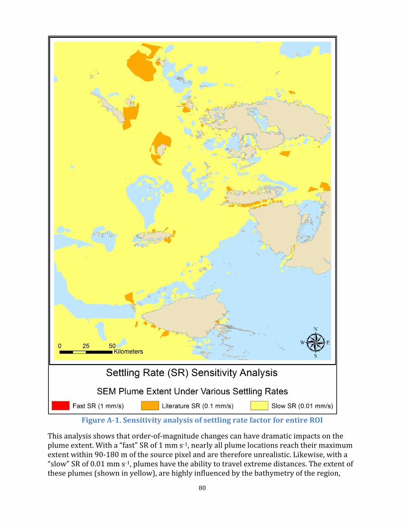
80
Figure A-1. Sensitivity analysis of settling rate factor for entire ROI
This analysis shows that order-of-magnitude changes can have dramatic impacts on the plume extent. With a “fast” SR of 1 mm s-1, nearly all plume locations reach their maximum extent within 90-180 m of the source pixel and are therefore unrealistic. Likewise, with a “slow” SR of 0.01 mm s-1, plumes have the ability to travel extreme distances. The extent of these plumes (shown in yellow), are highly influenced by the bathymetry of the region,

81
where deeper depths allow further traveling distances. With this result, it is important to remember that as plume extents increase in area, sediment concentration hypothetically decreases. While this relationship is not captured in this model, future studies linking sediment concentration and marine ecosystem impact could potentially determine a cut-off point for a minimum SR parameter.
Suspension Maintenance Factor
In the same manner, we conducted a sensitivity analysis for the Suspension Maintenance Factor (SMF) to better understand the influence of this parameter on plume extent. While constant terminal SRs can be considered the dominant process in deep water, the SMF was developed to approximate the effects of additional energy sources on the suspension of sediment as a function of depth. These effects include near-shore dynamic processes such as sediment re-suspension, wave turbulence, and upwelling that are not captured within the HYCOM data. This parameter was developed because during initial model runs shallow water surrounding river-mouths created extremely small plumes. Based on what we know about plume dynamics, constant terminal SRs are not a reliable measure in shallow water due to these additional influences. This has been confirmed in recreational aerial imagery of the region, which shows sediment kept in suspension for great distances along the coast in shallow water. Because this additional parameter is an approximation of many complex and dynamic coastal processes, it is up to the user to define which value is best. If future data were collected on actual plume extents and the relationship between deep and shallow water transport could be better understood, both the SR and the SMF could be tuned to represent a suite of local conditions.
Due to these uncertainties, we modeled how plume extents change as the SMF changes. We modeled three different SMF scenarios: (1) no SMF, (2) a SMF of base 10 (Equation A-1) and (3) a SMF of base 100 (Equation A-2). As discussed in the methods, increasing the SMF decreases the SR as a function of depth. This essentially transforms the SR and creates a new SR for every 10 m isocline. We started this analysis assuming the “literature” SR of 0.1 mm s-1, which was used in our final analysis. This relationship can be seen in Figure A-2 below. The effect of the Low and High SMF scenarios diminishes with depth and approaches the original static SR around -50 m in depth.
Equation A-1.
[ ]
Equation A-2.
[ ]
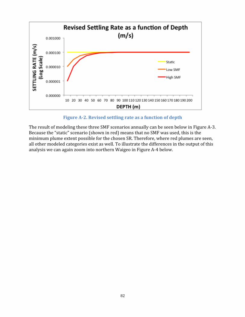
82
Figure A-2. Revised settling rate as a function of depth
The result of modeling these three SMF scenarios annually can be seen below in Figure A-3. Because the “static” scenario (shown in red) means that no SMF was used, this is the minimum plume extent possible for the chosen SR. Therefore, where red plumes are seen, all other modeled categories exist as well. To illustrate the differences in the output of this analysis we can again zoom into northern Waigeo in Figure A-4 below.
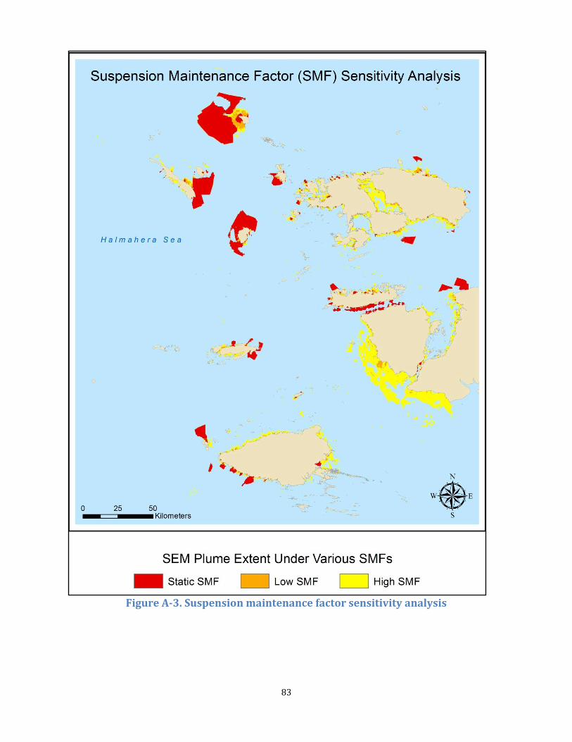
83
Figure A-3. Suspension maintenance factor sensitivity analysis

84
Figure A-4. Suspension maintenance factor sensitivity analysis for northern Waigeo
Figure A-4 shows how the implementation of the SMF increases plume extent in shallow water, allowing increased transport along the coast. To improve upon our analysis, implementing different SMFs for different months could provide a more appropriate connection between seasonal wave/coastal energy and sediment plume extent. For example, increased sediment delivery during monsoonal conditions is also usually accompanied by increased wave heights and long-shore transport. Therefore, the relationship between sediment extent and associated impact could be refined throughout the year.