Labor Market Fluidity and Human Capital Accumulation

Niklas Engbom∗

December, 2021

Abstract

Using panel data from 23 OECD countries, I document that wages grow more over the life-cycle in

countries where job-to-job mobility is more common. A life-cycle theory of job shopping and accumu-

lation of skills on the job highlights that a more fluid labor market allows workers to faster relocate to

jobs where they can better use their skills, incentivizing accumulation of skills. Lower labor market

fluidity reduces life-cycle wage growth by 20 percent and aggregate labor productivity by nine per-

cent across the OECD relative to the US. I derive a set of testable predictions for training and confront

them with comparable cross-country training data, finding support for the theory.

∗New York University, CEPR, NBER and UCLS. Email: nengbom@stern.nyu.edu. First draft: August, 2015. This paperpreviously circulated under the title "Worker Flows and Wage Growth over the Life-Cycle: A Cross-Country Analysis." Iam grateful for the generous support and advice of Richard Rogerson. I thank Mark Aguiar, Jorge Alvarez, Adrien Bilal,Carlos Carrillo-Tudela, Matthias Doepke, Domenico Ferraro, Victoria Gregory, Veronica Guerrieri, Gregor Jarosch, Greg Ka-plan, Burhan Kuruscu, Guido Menzio, Claudio Michelacci, Ben Moll, Chris Moser, Diego Restuccia, Todd Schoellman, VenkyVenkateswaran, Gustavo Ventura, Gianluca Violante, and seminar participants at Arizona State, CEMFI, Einaudi, FRB Rich-mond, Georgetown, ITAM, Melbourne, MIT, Princeton, Toronto and the SED. I also thank Eurostat for granting me access to theECHP and EU-SILC data sets. The results and conclusions in this paper are mine and do not represent Eurostat, the EuropeanCommission or any of the national statistical agencies whose data are used. All errors are my own.

1 Introduction

A large literature studies differences in labor market flows across countries. This research finds that such

flows vary markedly between countries, and that policies and institutions that impede such flows may

lead to misallocation of factors of production.1 The literature has, however, tended to focus on the effect

of such policies on firms’ job creation and destruction decisions, with less attention paid to their impact

on worker flows and the behavior of workers. Yet workers’ responses to such large differences in the

functioning of the labor market may have a first-order effect on aggregate economic outcomes.

In this paper, I quantify the consequences of cross-country differences in labor market fluidity on

workers’ careers, where I measure labor market fluidity as how frequently workers make job-to-job (JJ)

transitions. In particular, I argue that greater labor market fluidity encourages individuals to accumulate

skills on-the-job. The reason is that it improves their ability to locate a job where their skills are more

useful. Consequently, labor market fluidity facilitates life-cycle wage growth, both by allowing workers

to move toward jobs that reward their skills better and by inducing them to grow their skills more.

I proceed in three steps. In the first part of the paper, I establish a series of new facts on cross-country

differences in life-cycle careers. To that end, I build an internationally comparable worker-level panel

data set covering close to a million observations for over 20 years across 23 OECD countries. The data

suggest wide dispersion across countries in labor market flows and life-cycle wage growth. For instance,

labor market fluidity differs by a factor of 2.5 across countries, while workers experience substantially

greater life-cycle wage growth in some countries, mirroring findings in Lagakos et al. (2018).

My main empirical finding is that wages grow more over the life-cycle in more fluid labor markets.

The panel dimension of my data allows me to rule out that this is driven by differential selection patterns

over the life-cycle across countries by controlling for individual-fixed effects. Moreover, by standardiz-

ing education and occupation classifications across countries, I conclude that differences in workforce

composition along such dimensions across countries do not drive the patterns. Yet it is not entirely sur-

prising that wages grow more over the life-cycle in countries where JJ mobility is more common, as such

transitions are typically associated with wage gains. Indeed, I document that wages, in a residual sense,

rise by 5–6 percent more in years when a worker makes a JJ move, and that the magnitude of these

gains is uncorrelated with labor market fluidity. Nevertheless, in an accounting sense, accumulating

such wage gains over the life-cycle, they cumulatively account for only about a quarter of the steeper

life-cycle wage growth in more fluid labor markets. That is, most of the steeper life-cycle wage growth

in more fluid labor markets arises within jobs, as opposed to between jobs.

1See, e.g. Bentolila and Bertola (1990), Hopenhayn and Rogerson (1993), and Ljungqvist and Sargent (1998, 2008).

1

Although novel and intriguing, these correlations fall short of a quantitative assessment of the impact

of differences in labor market fluidity on workers’ careers. For this purpose, I propose in the second

part of the paper a tractable life-cycle theory of accumulation of skills in a frictional labor market. The

framework combines two benchmark models of worker career outcomes: endogenous accumulation

of human capital on-the-job as in Ben-Porath (1967) and a job ladder model in the spirit of Diamond

(1982)–Mortensen and Pissarides (1994). While on their own each framework is well understood, their

combination offers a rich set of testable predictions for how human capital accumulation and job mobility

interact. The marginal product of a worker’s human capital differs across firms, but frictions in the labor

market prevent workers from immediately relocating to their most productive use. A key difference to

an earlier literature on training in frictional labor markets is that I allow workers to move directly from

one employer to another without an intervening spell of unemployment (Acemoglu, 1997; Acemoglu

and Pischke, 1998, 1999b).2 By leaving a worker in a favorable bargaining position with a new employer,

the nature of such JJ mobility differs from mobility through unemployment. A young worker enters

the labor market with few skills and in a job that does not utilize her skills particularly well. Through

on-the-job training, she gradually builds her skills. Other firms try to poach her, such that over time she

reallocates toward jobs that use her skills efficiently—she climbs the job ladder.

I examine in the model the impact on workers’ careers of wedges to firms’ cost of creating jobs,

motivated by a large literature that argues that policies such as, for instance, business regulations, labor

taxes and employment protection legislation (EPL) serve to raise the cost to firms of hiring (Hopenhayn

and Rogerson, 1993; Pries and Rogerson, 2005). Such wedges reduce labor market fluidity. As workers

have a harder time finding a job that uses their skills efficiently, the value of human capital declines.

Workers respond by accumulating less human capital, such that the stock of human capital falls.

I calibrate the model to match key life-cycle outcomes in the US as a typical high-fluidity country.

As in the data, JJ mobility declines with age, as workers gradually settle into jobs that use their skills

efficiently. Wages grow rapidly early in careers, as young workers climb the job ladder and face high

marginal returns to training. My estimates imply that human capital is the most important source of

life-cycle wage and productivity growth, contributing 25 log points between age 25 and 50. Growth in

match productivity is a close second. Wages also grow as the arrival of outside offers allows workers to

bargain up their pay, and due to a declining share of time devoted to training over the life-cycle.

To quantify the impact of labor market fluidity on workers’ careers, I introduce in the calibrated

model wedges to firms’ cost of creating jobs such that the model matches the cross-country variation in

2Acemoglu and Pischke (1998) briefly discuss the effect of allowing for poaching—what they refer to as raids—noting that"whether raids are possible or not, may have important consequences for training." They do not pursue this further, though.

2

labor market fluidity. By holding all other parameters fixed at their estimated US values, this approach

isolates the impact of labor market fluidity on workers’ careers. Differences in labor market fluidity

account for 50 percent of the steeper life-cycle wage growth in more fluid labor markets across my sample

of OECD countries. Match productivity grows less over the life-cycle in less fluid labor markets as

workers climb the job ladder slower, accounting for a third of the impact of labor market fluidity on

wage growth. Less human capital accumulation accounts for another third, with the remainder due to

slower growth in the share of match output appropriated by workers and less training early in careers.

Across the OECD, aggregate labor productivity is nine log points lower relative to the US. In summary,

my findings highlight that policies and regulations that reduce labor market fluidity in turn have large

negative consequences on both workers’ life-cycle wage growth and aggregate economic outcomes.

The theory makes rich predictions for how training varies both across and within countries. In the

third part of the paper, I confront key predictions of the model with cross-country panel data on on-the-

job training and job mobility. Using these data, I uncover several patterns consistent with the theory.

First, workers spend more time on training in countries with a more fluid labor market and in occu-

pations and sectors with relatively higher labor market fluidity within countries. Second, conditional

on worker-fixed effects, workers train more when employed at larger, higher paying employers. This

pattern is consistent with the predictions of the theory that, ceteris paribus, workers train more in more

productive, higher paying firms, as such firms afford them greater use of their skills. Third, workers

in less fluid labor markets train disproportionately less at small, low paying employers. According to

the theory, this is because in less fluid labor markets workers currently in low productive firms have a

harder time moving to jobs where they can better use their skills. Expecting this, they train less.

Most of this paper purposefully avoids taking a strong stand on the exact policies that result in dif-

ferences in labor market fluidity, which as noted above has been extensively studied in the literature.

Instead, I focus on the implication of such differences for worker behavior, in the spirit of Restuccia and

Rogerson (2017, p.170)’s argument that "whereas much of the literature has focused on static misallo-

cation, we think the dynamic effects of misallocation deserve much more attention." That being said, I

provide reduced-form empirical evidence that labor market fluidity is negatively correlated with poli-

cies and regulations that raise the cost on firms of doing business, consistent with the literature (Lazear,

1990; Fonseca et al., 2001). Moreover, I find that the wedges required to match differences in labor mar-

ket fluidity are also quantitatively consistent with cross-country differences in the cost of starting firms

estimated by the World Bank. Finally, I exploit a significant reduction in EPL in Spain in 1994–1995 to

show that the fall in EPL was associated with an increase in labor market fluidity, as well as a fall in

wages of labor market entrants, a steepening of subsequent wage growth, and an increase in vocational

3

training. These empirical patterns are quantitatively consistent with the predictions of the model.

Related literature. A vast literature documents cross-country differences in labor market outcomes.3

Whereas much work has focused on hours worked or unemployment (Nickell, 1997; Bick et al., 2018;

Feng et al., 2020), less work assesses differences in wage growth and labor market flows, particularly JJ

flows. Hobijn and Sahin (2009) document flows in and out of unemployment across 27 OECD countries,

while Jolivet et al. (2006) find JJ mobility patterns consistent with this paper across 11 countries for 1994–

1997. Lagakos et al. (2018) show that richer countries have steeper life-cycle wage growth across 18

countries at different stages of development, while Donovan et al. (2020) document differences in labor

market flows across rich and poor countries.4 Guner et al. (2018) document and propose a theory that

accounts for steeper earnings growth for managers relative to non-managers in rich countries.

Recent work combines human capital and search in studies of workers’ careers (Bagger et al., 2014),

building on seminal work by Becker (1962), Ben-Porath (1967), Diamond (1982), Mortensen and Pis-

sarides (1994), and Burdett and Mortensen (1998). This literature typically models human capital as

exogenous via learning-by-doing (Yamaguchi, 2010; Burdett et al., 2011, 2020), although Rubinstein and

Weiss (2006), Fu (2011) and Bowlus and Liu (2013) are important exceptions. I instead follow Ben-Porath

(1967) to model training as a choice. This approach provides rich insights into how search and hu-

man capital accumulation interact. Herkenhoff et al. (2018) study learning through interactions with

co-workers.5 Wasmer (2006) provides a theory of on-the-job accumulation of skills and search, which

highlights that high turnover increases incentives to accumulate general rather than firm-specific skills.

Relative to him, I abstract from firm-specific skills, motivated by a recent literature that questions the

importance of such skills (Kambourov and Manovskii, 2009; Lazear, 2009). Indeed, I provide novel ev-

idence consistent with this recent view based on the joint dynamics of on-the-job training and worker

mobility. While the theory in this paper is less general than Wasmer (2006), I offer a quantitative assess-

ment of the impact of labor market fluidity on cross-country differences in career outcomes, including

direct empirical support for the predictions of the model based on panel micro data on training.

In Michelacci and Pijoan-Mas (2012), workers accumulate skills by working longer hours. They show

that an increase in wage inequality accounts for two-thirds of the increase in average hours worked in

3Another voluminous literature assesses the sources of cross-country income differences. Manuelli and Seshadri (2014) isclosest to this paper in that they also allow for on-the-job accumulation of skills, but abstract from labor market frictions.

4Consistent with this paper, the latter find that richer countries have higher JJ flows among a set of developed countries—forinstance, their Table 2 "provides the regression estimates from a sample that includes only EU countries, Switzerland, the U.K.,and the United States. For this sample, we also find a positive relationship between labor market flows and development"(Donovan et al., 2020, p.14). In contrast, developing countries are characterized by higher labor market flows.

5In Engbom (2020), I propose a theory of search and entrepreneurship to study the impact of demographic change, whereasthe current paper assesses how search and training interact with a focus on cross-country patterns.

4

the US since 1970. I abstract from an intensive margin of labor supply—motivated by a lack of corre-

lation between labor market fluidity and average hours worked per week across countries—to instead

model human capital accumulation following Ben-Porath (1967). Lentz and Roys (2016) incorporate risk

aversion in a model of endogenous on-the-job accumulation of skills and labor market search. Although

their focus is not on understanding cross-country patterns, they show that lower labor market frictions

encourage training, mirroring findings in this paper. Flinn et al. (2017) use NLSY 1997 training data to

discipline a rich theory of training and search. While I do not use training data in estimation, I use such

data to validate the predictions of the model across countries. Other important differences include this

paper’s focus on cross-country patterns and the introduction of a proper notion of a life-cycle.

Doepke and Gaetani (2020) develop a quantitative life-cycle model of search and training to under-

stand the different evolution of the college premium in the US and Germany over the past decades.

Relative to them, I incorporate and put center stage JJ mobility, motivated by the large cross-country

differences in such flows that I document. Gregory (2019) offers a rich framework in which firms differ

in both their productivity and learning environment.6 While the current paper also predicts that work-

ers grow their skills more in some firms—consistent with her reduced-form patterns—such differential

growth rates arise here through workers’ and firms’ optimizing behavior. In addition, I use data on

training on-the-job to establish new facts on how training varies across jobs.

This paper is organized as follows. Section 2 establishes a series of novel facts on cross-country dif-

ferences in life-cycle careers, while Section 3 proposes a theory of endogenous accumulation of skills in a

frictional labor market to interpret the empirical patterns. Section 4 estimates the model targeting the US

as a typical high-fluidity country, and uses it to quantify the impact of labor market fluidity on workers’

careers as well as ultimately aggregate outcomes across countries. Section 5 derives and contronts key

predictions of the theory with standardized training data across countries. Section 6 discusses factors

behind cross-country differences in labor market fluidity, while Section 7 concludes.

2 Motivating facts

This section contributes to the literature by establishing a set of new facts on life-cycle labor market out-

comes across countries. To that end, I build an internationally comparable worker-level panel data set

covering 23 OECD countries based on the following sources: the US Panel Study of Income Dynamics

(PSID) 1994–2015; the German Socio-Economic Panel (GSOEP) 1991–2011; the British Household Panel

Survey (BHPS) 1991–2008; the European Community Household Panel (ECHP) 1994–2001; and the Eu-

6Her work, this paper and much of the macro-labor literature share that there is no distinction between a firm and a match.

5

ropean Union Statistics on Income and Living Conditions (EUSILC) 2003–2014. While a cross-country

comparison inevitably is subject to issues of comparability, an important advantage of these data sets is

that they are modeled on the PSID, facilitating the comparison.7 See Appendix A.2 for details.

2.1 Sample selection

I focus on men, as female labor force participation likely varies across countries for reasons that the the-

ory in the next section abstracts from. To limit the impact of issues associated with labor force entry and

retirement, I primarily focus on ages 25–54, but present additional samples as robustness. As I discuss in

Appendix A.3, male labor force participation rates are consistently high across countries between ages

25–54. Moreover, there is no statistically significant correlation between labor force participation rates

and labor market fluidity, either at the aggregate level, at age 25 or at age 54. Additionally, I drop obser-

vations with missing year of birth or employment status, as well as individuals whose reported year of

birth deviates by more than five years across panel years. This excludes very few observations.

I focus on employees and flows in and out of unemployment, as the theory also abstracts from self-

employment and non-participation. Flows in and out of non-participation are small, however, and do

not vary systematically with labor market fluidity among prime aged men. I include all wage employees,

regardless of full-time status, but similar results hold among those working 30+ hours a week. In my

main analysis, I do not condition on being in the private sector, partly because the EUSILC does not

make available sector to researchers. Appendix A.4 argues that the public-private distinction is unlikely

to be a main force driving the cross-country patterns documented here (among prime aged men).

My analysis focuses primarily on 13 developed Western European countries and the US for which

I have 15 or more years of data. I report robustness results including an additional 10 OECD countries

for which I have fewer years of data.8 The core annual sample includes over six hundred thousand

observations, with another two hundred thousand observations for the other OECD countries.

2.2 Variable definitions

I construct two samples. The first is an annual sample used in my wage analysis. The wage is total gross

labor income in the prior calendar year divided by annual hours worked, constructed as the product of

7For this reason, I prefer to use the PSID in my main analysis of worker flows. Appendix A.1 shows that the resulting flowsare broadly consistent with those in the US Survey of Income and Program Participation (SIPP).

8The EUSILC also contains a few years of data for Bulgaria, Cyprus, Malta, Romania and Serbia. I have confirmed that myfindings hold also including these countries, but I prefer to focus on the set of relatively comparable OECD countries.

6

weeks worked times usual weekly hours.9 I top-code weekly hours at 98 hours to be consistent with the

PSID. I include in labor income also income from self-employment to be consistent with the BHPS, which

does not distinguish sources of labor income. I do, however, focus on those who are wage employed at

the time of the survey—henceforth employees.10 I convert nominal values to real 2004 local currency

using the national CPI, then to real US dollars using the PPP-adjusted exchange rate in 2004.

The second sample is a monthly data set, which I use to estimate labor market flows. The surveys ask

for labor market status in each month during the prior calendar year. By linking subsequent years, I obtain

labor force status in each month during the 12 months prior to the survey month. In particular, a worker

is said to make an EU transition if she is employed in the current month but unemployed in the subse-

quent month. She makes an UE transition if she is unemployed in the current month but employed in the

subsequent month.11 The available data sets do not allow for the construction of a satisfactory monthly

measure of JJ mobility, because the surveys in general ask for information on only (up to) two employ-

ment spells in the prior year. As a consequence, at most one JJ move can be observed during the past 12

months, even though the worker might have made multiple transitions. For young, highly mobile work-

ers in particular, this restriction is not innocuous. Hence, I instead construct a consistent measure of JJ

mobility across countries as the fraction of employees who started working for their current employer

at some point in the past 11 months while having had employment as the main employment status in

every of the past 12 months. Subject to one caveat, this measure accounts for intervening months of non-

employment between job switches—it is not equivalent to the fraction of employed workers who were

at a different employer 12 months earlier. The one caveat is that it does not rule out short intervening

spells of unemployment, as I only observe main employment status in a month. Because flows in and

out of unemployment are so low, however, I doubt time aggregation majorly biases my results.12

I standardize year of birth to the modal value across panel years, education into two groups—less

than college or college or more—based on an individual’s highest reported degree across panel years,

9In the PSID, each subcomponent of total income is top-coded at separate thresholds that vary across years. I use a Paretoimputation to top-coded subcomponents in each year before I sum each component to get total income (Heathcote et al., 2010).The BHPS records income and hours from September to September instead of by calendar year.

10Robustness exercises suggest that differences in self-employment income among wage employees are third-order withrespect to the patterns documented here (available for all countries but the UK).

11The PSID does not allow a distinction between wage and self-employment in the monthly calendar of events, and henceto be consistent all monthly flows include the self-employed as employed. In the other data sets as well as in the US SIPP,though, flows from employment to (and from) self-employment are an order of magnitude smaller than those to (and from)unemployment, so I believe that this issue is second-order.

12As part of the estimation in Section 4, I simulate a monthly approximation to the underlying continuous time model. Ihave alternatively simulated a weekly model and aggregated that up to the monthly level. It has a second-order impact onmy measure of JJ mobility, precisely because flows in and out of unemployment are so low. The fact that flows in and out ofunemployment are estimated to be much lower in panel data relative to primarily cross-sectional data such as the US CurrentPopulation Survey has been long recognized in the literature, driven by employment status classification error (Abowd andZellner, 1985; Poterba and Summers, 1986). See Appendix A.1 for more details and a comparison with the US SIPP.

7

and occupation into 10 internationally comparable, aggregate occupation groups based on ISCO-88.

I construct life-cycle wage profiles by regressing separately by country the log hourly real wage of

individual i in year t, wit, on age effects, Ait, year effects, Yt, and individual fixed effects, Ii,

wit = Ait + Yt + Ii + ε it (1)

The inclusion of individual fixed effects in regression (1) addresses important concerns about differences

in sample attrition across countries biasing the cross-country comparison of life-cycle wage growth.

In my benchmark, I compute wage growth by age. But I also report results below controlling for

education—isomorphic to wage growth by potential experience—with similar results.

Whenever an individual gets one year older, time also increases by one year, and vice versa. That is,

age, time and individual fixed effects are collinear. Hence, a restriction is needed to identify regression

(1). I follow Heckman et al. (1998) and Lagakos et al. (2018) in imposing that wages depreciate at some

rate d after some age A. This restriction is sufficient to separate individual, time and age effects. Effec-

tively, fluctuations in wages among individuals older than A identify the year effects. The age effects

can then be recovered from within-individual fluctuations in wages among those aged less than A.

Appendix A.5 plots JJ, EU and UE mobility as well as wages over the life-cycle across countries.

2.3 Wages grow more over the life-cycle in more fluid labor markets

Panel A of Figure 1 plots life-cycle wage growth against labor market fluidity across the core set of 13

countries. Wages grow substantially more over the life-cycle in more fluid labor markets. For instance,

wages rise by 75 log points in the US between ages 25–54, but only by 30 log points in Italy. Panel B

shows that similar results hold when including the additional 10 countries with fewer years of data,

with a correlation coefficient between life-cycle wage growth and labor market fluidity of around 0.8.

One possible factor behind these patterns is differences in workforce composition. To assess this, I

consider an augmented version of regression (1) that instead pools all countries and years,

wit = α fluidityc × ait + ∑e

βeeit × ait + Ii + Yt + Ait + ε it (2)

As above, wit is the log real hourly wage, Ii are individual fixed effects, Yt are year effects, and Ait are

restricted age effects. The coefficient α captures the covariance between life-cycle wage growth and labor

market fluidity, controlling for separate age slopes for two education groups or 10 occupation groups

(minus one due to collinearity). I renormalize the provided survey weights such that each country in the

8

aggregate receives a total weight of one,13 and cluster standard errors by country.

Table 1 presents regression results from several specifications, including allowing for wages to fall

late in life and extending the sample to include all workers aged 22–59. Appendix A.6 shows that similar

results hold for the full sample of 23 countries. Confirming the pattern in Figure 1, there is a strong,

statistically significant positive correlation between labor market fluidity and life-cycle wage growth

in the baseline specification. While college graduates, for instance, experience greater life-cycle wage

growth, differences in educational or occupational composition across these developed countries are

much too small to change this conclusion. Allowing for a different depreciation rate late in careers

makes virtually no difference to the point estimate. Moreover, extending the sample to start at age 22

and/or include those up to age 59 does not change the conclusion. In additional results I reach the same

conclusion including workers up to age 64, including instead setting A = 55.

FIGURE 1. LIFE-CYCLE WAGE GROWTH AND LABOR MARKET FLUIDITY

(A) CORE COUNTRIES (B) ALL COUNTRIES

Note: Male employees aged 25–54. Labor market fluidity: Share of employees who started working for their current employer at some pointin the past 11 months while having been employed in all of the past 12 months. Employment in the past 12 months includes self-employmentdue to data limitations. Constructed by first collapsing the data to the country-age-year level using the provided survey weights, then to thecountry-level. Life-cycle wage growth: Log hourly real wage profile based on regression (1) with worker fixed effects, time effects and ageeffects restricted to zero growth after age 50. Source: BHPS, ECHP, EUSILC, GSOEP and PSID 1991–2015.

It is, perhaps, not surprising that wages grow more in countries where workers on average make

more JJ transitions, as such transitions typically involve a wage gain (Topel and Ward, 1992). Indeed,

Panel A of Figure 2 shows that across all countries, the average worker tends to experience greater

growth in wages in years when she made a JJ move. It projects the difference in median annual wage

growth between those who made a JJ move in the year and those who did not on labor market fluidity,

13For countries with observations in the ECHP and EUSILC, I adjust the weights such that each country-survey receives arelative weight equal to the number of years of data for that country in that survey, and the total weight for the country is one.

9

computed within age-year bins and subsequently aggregated to the country-level giving equal weight

to each year-age. I use the median to limit the impact of a few outliers.14 A JJ mover experiences 5.5

percent greater residual wage growth in a year relative to a stayer with the same age in the same year.

There is no systematic relationship between the wage gain upon a JJ move and labor market fluidity.

TABLE 1. LIFE-CYCLE WAGE GROWTH AND LABOR MARKET FLUIDITY

Panel A. Ages 25–54 Panel B. 1% depreciation Panel C. Ages 22–59

Baseline Educ Occup Baseline Educ Occup Baseline Educ Occup

α 0.244*** 0.217** 0.224*** 0.244*** 0.217** 0.224*** 0.261*** 0.230*** 0.238***(0.074) (0.076) (0.069) (0.074) (0.076) (0.069) (0.069) (0.069) (0.065)

N 336,349 334,415 323,888 336,349 334,415 323,888 393,910 391,042 379,094

Note: Male employees. Panel A. Wages restricted to not grow after age 50. Panel B. Ages 25–54 with wages restricted to depreciate 1% annuallyafter age 50. Panel C. Wages restricted to not grow after age 50. Labor market fluidity: Share of employees who started working for their currentemployer at some point in the past 11 months while having been employed in all of the past 12 months. Employment in the past 12 monthsincludes self-employment due to data limitations. Constructed by first collapsing the data to the country-age-year level using the providedsurvey weights, then to the country level. α: Fluidity-age interaction in regression (2) with worker fixed effects, time effects and restricted ageeffects. Standard error below are clustered at the country-level. ** statistically significant at 5%; *** statistically significant at 1%. Source: BHPS,ECHP, EUSILC, GSOEP and PSID 1991–2015.

FIGURE 2. THE ROLE OF BETWEEN-JOB WAGE GROWTH

(A) WAGE GAIN IN YEAR OF JJ MOVE (B) BETWEEN VS WITHIN JOB

Note: Male employees aged 25–54. Panel A. Median annual wage growth of workers who made a JJ move in the past year relative to thosewho did not, computed within country-year-age groups and then collapsed to the country-level giving equal weight to each year-age. PanelB. Between-job: Product of the median wage gain from a JJ move and the average total number of JJ moves between age 25–54. Within-job:Difference between total wage growth between age 25–54 and the between-job component. Total wage growth based on (1) with worker fixedeffects, time effects and age effects restricted to be zero past age 50. All panels. Labor market fluidity: Share of employees who started workingfor their current employer at some point in the past 11 months while having been employed in all of the past 12 months. Employment in thepast 12 months includes self-employment due to data limitations. Constructed by first collapsing the data to the country-age-year level usingthe provided survey weights, then to the country level. Source: BHPS, ECHP, EUSILC, GSOEP and PSID 1991–2015.

Panel B uses the gain upon a JJ move to estimate the contribution of job shopping toward life-cycle

14Because the PSID turned biannual in 1997, the estimate of wage gains for the US relies only on years 1994–1997. As Ishow in Section 4, however, the wage gain upon a JJ move is similar in the SIPP for more recent years and I reach very similarconclusions if I approximate the annual wage gain after 1997 in the PSID with the bi-annual wage gain.

10

wage growth. I compute between-job life-cycle wage growth by multiplying the wage gain from a JJ

move with the average number of JJ moves a worker makes between age 25–54.15 I compute within-

job life-cycle wage growth as the difference between total wage growth and between-job wage growth. I

stress that no structural interpretation should be assigned to the components—it is simply an accounting

decomposition. Less than a quarter of the steeper life-cycle wage growth in more fluid labor markets

is accounted for by between-job wage growth. Because the average wage gain is not correlated with

fluidity, the steeper between-job wage growth in more fluid labor markets is entirely driven by the higher

frequency of moves. Hence, while the between-job component is non-trivial, the majority of the steeper

life-cycle wage growth in more fluid labor markets takes place within-jobs.

2.4 Discussion

Before I go to the model, I establish some additional empirical patterns that help guide the analysis.

Entry wages. Table 2 regresses wages of labor market entrants on labor market fluidity, with or without

controls. Because this exercise assesses level differences, I cannot control for worker fixed effects. Entry

wages are lower in more fluid labor markets, although not statistically significantly so. Quantitatively,

entry wages are 2–6 percent higher in the least fluid labor market relative to the US. Controlling for real

GDP per hour in 2004 PPP-adjusted US dollars makes the pattern more pronounced.16

What workers grow their wage more? Assessing what workers grow their wages more in more fluid

labor markets may shed further light on potential driving forces behind the patterns. Panel A of Figure

3 re-estimates life-cycle wage growth based on (1) separately by education group, and projects it on

labor market fluidity, also computed separately by education group. College educated workers grow

their wage more over the life-cycle in all countries. Moreover, the gradient with labor market fluidity is

steeper among college graduates (although Italy is a peculiar outlier).

Panel B considers an augmented version of the pooled regression (2) that includes a linear in an

occupation’s wage rank, as well as its interaction with age, fluidity and age times fluidity. I rank oc-

cupations within each country-year, and then assign the occupation its (unweighted) average across

country-years.17 Higher wage occupations experience steeper life-cycle wage growth. Moreover, they

15While there is a life-cycle profile to the wage gains upon a JJ move, this computation relies only on life-cycle averages. Thatis, it makes no difference to the total to use the age-specific wage gains (although it does matter for the timing of the gains).

16I am not, however, convinced that doing so makes sense. To the extent that the labor share does not covary systematicallywith fluidity (which it does not), controlling for labor productivity is isomorphic to controlling for the average wage. Hencewith such a control, the steepness of life-cycle wage profiles and entry wages are the flip side of the same coin.

17The resulting ranking makes intuitive sense, with engineers and doctors ranked the highest and laborers ranked the lowest.

11

experience disproportionately steeper wage growth in more fluid labor markets relative to lower wage

occupations, although the pattern is not statistically significant (p-value of 0.25). I conclude from these

two exercises that the cross-country correlation between life-cycle wage growth and labor market fluid-

ity is not driven by low skilled, low wage workers. At face value, this speaks against explanations based

on minimum wages or unions, which typically impact lower skilled workers the most.

TABLE 2. ENTRY WAGES AND LABOR MARKET FLUIDITY

Year Educ Occup GDP

α -0.891 -0.358 -0.637 -3.105*(2.795) (2.921) (2.722) (1.721)

N 21,266 20,342 20,200 21,266

Note: Male employees 21–24. Log hourly real wage in 2004 PPP-adjusted USD. Year: Year controls. Educ: Year and education controls. Occup:Year and occupation controls. GDP: Year and GDP per hour controls (in 2004 PPP-adjusted USD). Labor market fluidity: Share of employeeswho started working for their current employer at some point in the past 11 months while having been employed in all of the past 12 months.Employment in the past 12 months includes self-employment due to data limitations. Constructed by first collapsing the data to the country-age-year level using the provided survey weights, then to the country-level. Standard errors are clustered at the country-level. * significant at10%. Source: BHPS, ECHP, EUSILC, GSOEP and PSID 1991–2015.

Inequality. Patterns for inequality may provide additional guidance regarding the forces at work. For

instance, Guvenen et al. (2013) emphasize that progressive taxation reduces life-cycle wage growth and

inequality, which may be correlated with labor market fluidity. Panel A of Figure 4 relates labor market

fluidity to the standard deviation of log residual wages. I focus here on residual inequality, because that

is what the theory in the next section is about. Appendix A.7 contains additional results.

Panel B graphs life-cycle growth in inequality against fluidity, where the former is the difference

in standard deviation of residual log wages at age 50–54 relative to at age 25–29. Neither the level of

inequality nor its change over the life-cycle is systematically related to labor market fluidity. While

inequality in general rises over the life-cycle across these countries, it is primarily accounted for by

increasing dispersion across education and occupation groups. Within groups, the increase in inequality

is less pronounced, even in the US. I provide a further discussion and robustness in Appendix A.7.

Voluntary versus involuntary. The data sets also include information on the reason for separation,

which I standardize into those who quit the job versus the firm initiated the separation, which I some-

what loosely refer to as an involuntary separation. Panel C shows that, if anything, the share of quits

among JJ movers is higher in more fluid labor markets. Hence, the higher JJ rate is not driven by more

involuntary movers. The distinction between an employer initiated separation and a quit, however, is

murky. Indeed, the model in the next section predicts that separations are bilaterally optimal, with no

12

theoretical distinction between a quit and the employer letting the worker go. For this reason, I prefer to

use the overall measure of JJ mobility as my benchmark.

FIGURE 3. WAGE GROWTH AND LABOR MARKET FLUIDITY BY EDUCATION AND OCCUPATION

Interaction with occupation’s wage rank

fluidity × age 0.222***(0.070)

occupation wage rank -0.021***(0.006)

occupation wage rank × fluidity -0.122(0.163)

occupation wage rank × age 0.002***(0.001)

occupation wage rank × fluidity × age 0.017(0.014)

N 359,394

Note: Male employees aged 25–54. Left panel. Life-cycle wage growth based on regression (1) separately by country and education groupswith age effects restricted to not grow past age 50. Right panel. Pooled regression based on (2) with a linear in an occupation’s wage rank (10occupations), as well as its linear interaction with age, fluidity and fluidity times age. Labor market fluidity: Share of employees who startedworking for their current employer at some point in the past 11 months while having been employed in all of the past 12 months. Employmentin the past 12 months includes self-employment due to data limitations. Constructed by first collapsing the data to the country-age-year levelusing the provided survey weights, then to the country-level (in the left panel separately by education groups). Source: BHPS, ECHP, EUSILC,GSOEP and PSID 1991–2015.

The boundary of the firm. My measure of fluidity captures only mobility between firms. Hence, less

mobility across firms may be compensated for by higher mobility within firms. To the extent that large

firms offer greater scope for within-firm mobility, this scenario may be particularly plausible if firms are

smaller in more fluid labor markets. Panel D, however, shows that a larger share of workers work at

large firms in more fluid labor markets.18 At face value, this suggests that the higher mobility rates in

some countries is not driven by greater fragmentation of firms in such countries.

Other factors. Panel E shows that labor market fluidity is not correlated with PISA test scores. Together

with the facts that my results remain unchanged when controlling for education or occupation-specific

age slopes and that my core sample includes only highly developed OECD countries, this observation

leads me to discount the hypothesis that the steeper wage growth in more fluid labor markets is primarily

accounted for by workforce composition. Panel F shows that there is important cross-country variation

in the level of the unemployment benefit replacement rate, but it does not correlate strongly with labor

18My measure is the share of employment at firms with 50 employees or more. This is the only firm size measure consistentlyavailable across countries and years, and is not available for all countries (in particular, Germany is missing).

13

market fluidity. This pattern is consistent with the argument that other factors such as the cost of starting

a firm are more important determinants of labor market fluidity (Fonseca et al., 2001).

FIGURE 4. ADDITIONAL OUTCOMES

(A) LEVEL OF INEQUALITY (B) GROWTH IN INEQUALITY (C) SHARE OF VOLUNTARY JJ

(D) EMPL. SHARE, 50+ FIRMS (E) PISA TEST SCORE (F) UB REPLACEMENT RATE

Note: Men aged 25–54. Panel A. St.d. of residual log hourly wages, controlling for year-education-age and year-occupation effects separatelyby country. Panel B. Growth between ages 25–29 and 50–54 in st.d. of residual log hourly wages, controlling for year-education-age andyear-occupation effects separately by country. Panel C. Share of JJ transitions in which the worker quit as opposed to the firm initiated theseparation (restricted to employees only). Panel D. Share of employees working at firms with 50 or more workers. Firm size is only available inthe cross-sectional version of the EUSILC, missing from the BHPS (I use the ECHP/EUSILC), coded into non-comparable bins in the GSOEP,and only available in 1999 and 2003–2015 in the PSID. Panel E. PISA math test score. Panel F. Average short-term unemployment benefitreplacement rate as reported by the OECD. Panels A–D. Constructed by first collapsing the outcome variable to the country-year-age levelusing the provided survey weights, then to the country-level. Labor market fluidity: Share of employees who started working for their currentemployer at some point in the past 11 months while having been employed in all of the past 12 months. Employment in the past 12 monthsincludes self-employment due to data limitations. Constructed by first collapsing the data to the country-age-year level using the providedsurvey weights, then to the country-level. Source: BHPS, ECHP, EUSILC, GSOEP, OECD, and PSID 1991–2015.

Taking stock. Using detailed panel micro data, the above analysis establishes a set of new facts on

cross-country differences in career outcomes, the most prominent being that wages grow more over the

life-cycle in more fluid labor markets. This pattern is not accounted for by observable worker character-

istics, and the majority of it takes place within-jobs.

While novel and intriguing, however, these correlations do not settle the main question this paper

aims to answer: the impact of labor market fluidity on workers’ careers. To assess this, I now proceed to

propose a structural model that I use as a laboratory to isolate the impact of labor market fluidity as well

14

as explore its mechanisms. Section 5 returns to the data to test key predictions of the theory.

3 Model

At a conceptual level, a stylized job ladder model in the spirit of Burdett and Mortensen (1998) may suf-

fice to account for steeper wage growth in more fluid labor markets, as workers move up the job ladder

more. At the same time, a vast literature emphasizes the critical role played by human capital accumu-

lation in driving life-cycle wage and productivity growth (Becker, 1962; Mincer, 1974), suggesting that

it is important to understand how labor market fluidity impacts human capital accumulation. Hence, I

propose in this section an equilibrium model of careers that merges endogenous skill accumulation as in

Ben-Porath (1967) with a search model in the spirit of Bagger et al. (2014). The combination of search and

endogenous human capital accumulation leads to a rich set of predictions for how mobility and training

interact, which Section 5 finds empirical support for in both within-country and cross-country variation.

3.1 Environment

Time is continuous and infinite, there are no aggregate shocks and I focus on the long-run steady-state.

The economy consists of a unit mass of finitely-lived workers and some positive mass of firms. All agents

have linear preferences over a single output good discounted at rate ρ. Workers may allocate a unit of

time indivisibly toward working or not working. As unemployed, a worker enjoys flow value of leisure

b(a, h), which may depend on her age a and current human capital h.

Demographics. Workers are heterogeneous in initial skills h0 ∼ Λ and enter the labor market as un-

employed. They exit the labor market at age A and are replaced with an equal mass of young workers.

Upon retirement, workers enjoy a continuation value A that is independent of their labor market history.

Under linear utility, I may without loss of generality normalize the continuation value to zero, A = 0.

I neither model the distribution of initial skills Λ, the retirement age A, nor the continuation value A ,

and I later take these to be identical across countries. The lack of a systematic relationship between labor

market fluidity, on the one hand, and the overall labor force participation rate as well as that at age 25

and 54, on the other hand, leads me to focus my analysis elsewhere (see Appendix A.3 for details).

Production technology. The single good of the economy is produced by one worker-one firm matches,

and serves as the numeraire. A large number of potential firms may pay flow cost c in return for the

15

opportunity to meet with a worker. All costs are in terms of the final good. If a firm contacts a worker,

the two draw an idiosyncratic productivity z from exogenous offer distribution Γ.

Output of a match between a firm with productivity z and a worker with human capital h is y = zh,

i.e. human capital and technology are complements, as in Acemoglu and Pischke (1998) and Bagger et

al. (2014). As discussed further by Acemoglu (1997), a large empirical literature going back to Griliches

(1969) has found evidence of complementarities between physical and human capital. The critical aspect

of this assumption is the view that an individual may use her skills more efficiently in some jobs than

others—if an individual’s human capital is equally productive in all jobs, the predictions of this paper

would not go through. I hence also abstract from purely firm-specific human capital, consistent with the

evidence in Kambourov and Manovskii (2009) and Lazear (2009). Section 5 and Appendix E.4 document

cross-sectional patterns consistent with these two key assumptions.

Human capital accumulation. Employed workers may accumulate skills on-the-job. The human capi-

tal accumulation technology is independent of worker age a. Building on Ben-Porath (1967), if a worker

sets aside some fraction of her work time i toward building her skills, her human capital grows by

h =µ

η

(izh)η

, µ > 0, η ∈ (0, 1)

The opportunity cost of training is foregone production, izh. Human capital does not depreciate.19

In Ben-Porath (1967) there is no productivity dispersion, z, such that human capital grows by µ(ih)η/η

at cost ih. The current specification provides an extension to the case of employer heterogeneity. Note in

particular that a given amount of time, i, is assumed to grow human capital by more in a more produc-

tive firm. Absent this assumption, training falls in productivity, which is inconsistent with the positive

correlation between training, on the one hand, and firm size and firm pay, on the other, that I document

in Section 5 (conditional on worker fixed effects and time varying controls). In contrast, under the current

assumption, the model matches these empirical patterns well. The view that workers may learn more in

some jobs goes back to Rosen (1972) and more recently Jovanovic and Nyarko (1996) and Gregory (2019).

Labor market. The labor market is characterized by informational frictions that prevent the immediate

reallocation of a worker to the job that uses her skills the most efficiently. Both the unemployed and

employed search for jobs at random in a common labor market, in the latter case with exogenous relative

efficiency φ. Employed workers separate to unemployment at rate δ(z). The dependence on productivity

19An earlier version of this paper allowed for depreciation. As results were insensitive to (reasonable) variation in the extentof depreciation and the rate of depreciation was hard to identify from the available data, I opt to abstract from it.

16

z captures in reduced-form the view that less productive jobs are more likely to separate in response to

idiosyncratic shocks. It allows the model to match the decline in EU mobility with age.

If firms create V vacancies and workers search with aggregate efficiency S, the number of meetings

are, m = χVαS1−α, where α ∈ (0, 1) is the elasticity of matches with respect to vacancies. The job finding

rate is hence p = χ(V/S)α, while the worker finding rate of firms is q = χ(V/S)α−1.

I adopt the bargaining protocol of Dey and Flinn (2005) and Cahuc et al. (2006), which has become

a benchmark in the literature for its tractability and empirical relevance. Following Barlevy (2002) and

Bagger et al. (2014), wages are paid as a piece-rate r of net output, w = r(1 − i)zh. The worker and

firm bargain over the piece rate, r, and a training policy, i(a, h, z). The latter can be conditioned on the

observable states a, h and z. Under generalized Nash bargaining, the parties adopt the training policy

that maximizes their joint value, and split the proceeds.20 The firm and the worker can commit to the

contract {r, i(a, h, z)}, but commitment is limited in the sense that either party can force a renegotiation

when they have a credible threat to abandon the match under the existing contract.

This contracting structure implies that workers share in the cost of training through lower pay, con-

sistent with the fact that entry wages are lower in more fluid labor markets. More directly, Appendix

B.1 shows that workers—conditional on worker fixed effects and time-varying covariates—earn lower

hourly wages in years when they spend more hours on training.

3.2 Wages

Let U(a, h) be the value of unemployment to a worker of age a with human capital h, W(a, h, z, r, i) the

value of the worker when employed in a firm with productivity z when paid piece rate r and under

training policy i, F(a, h, z, r, i) the corresponding value to the firm, and J(a, h, z) the maximized joint

value of the match. I show below that the maximized joint value does not depend on how it is split.

Consider a meeting between an unemployed worker and a firm. The worker and firm bargain over

a training policy and a piece rate, leading them to adopt the training policy that maximizes their joint

value and a piece rate wu(a, h, z, i) determined by,

W(

a, h, z, wu(a, h, z, i), i)

= U(a, h) + β(

J(a, h, z)−U(a, h))

(3)

Consider next the case when an employed worker contacts a poaching firm. The new and the old

firm Bertrand compete for the worker, such that the worker’s outside option becomes the full value of

20Although the outcome is the same, Cahuc et al. (2006) microfound the bargaining protocol based on alternating offersRubinstein (1982).

17

the least productive match, J(a, h, z). Let we(a, h, z′, z, i) denote the pay of a worker who was employed

in firm z but gets poached by a firm z′ > z under training policy i. It is given by

W(

a, h, z′, we(a, h, z′, z, i), i)

= J(a, h, z) + β(

J(a, h, z′)− J(a, h, z))

(4)

If the poaching firm is less productive, z′ < z, the worker remains with her current firm, but possibly

with an updated piece rate given by the maximum of we(a, h, z, z′, i) and her previous wage, r. Let

r(a, h, z, r, i) be the lowest outside offer that leads to a renegotiation of the current contract, given by

J(a, h, r(a, h, z, r, i)) + β(J(a, h, z)− J(a, h, r(a, h, z, r, i))) = W(a, h, z, r, i).

Because age and human capital change over time, instances may arise when either the worker or

the firm would want to quit the match under the existing contract, even though the match has positive

surplus. In these instances, I assume that wages are rebargained according to (3).21

3.3 Value functions

Given an optimal training policy that maximizes the joint value as well as the splitting rules (3)–(4), the

value of unemployment solves the differential equation

ρU(a, h) = b(a, h) +∂U(a, h)

∂a+ pβ

ˆ ∞

0

(J(a, h, z)−U(a, h)

)+dΓ(z) (5)

subject to the terminal condition U(A, h) = 0, where x+ = max{x, 0}. The unemployed worker enjoys

flow value of leisure b(a, h). She meets potential employers at rate p, who are sampled from the offer

distribution Γ. If she accepts the job, she gets a share β of the surplus of the new match.

The value of a worker, W(a, h, z, r, i), evolves according to,

ρW(a, h, z, r, i) = r(1− i(a, h, z))zh +µ

η

(i(a, h, z)zh

)η ∂W(a, h, z, r, i)∂h

+∂W(a, h, z, r, i)

∂a(6)

+ φpˆ z

r(a,h,z,r,i)

(J(a, h, z′) + β(J(a, h, z)− J(a, h, z′))−W(a, h, z, r, i)

)dΓ(z′)

+ φpˆ ∞

z

(J(a, h, z) + β(J(a, h, z′)− J(a, h, z))−W(a, h, z, r, i)

)dΓ(z′)

+ δ(z)(

U(a, h)−W(a, h, z, r, i))

subject to W(A, h, z, r, i) = 0, W(a, h, z, r, i) ≥ U(a, h) and W(a, h, z, r, i) ≤ J(a, h, z). The worker receives

21In practice in the estimated model, these two cases are extremely rare, such that aggregate wage dynamics are essentiallyinvariant to alternative assumptions regarding how wages get rebargained in these scenarios.

18

a share r of net output today, grows her human capital and ages. At rate φp, she receives outside offers

from distribution Γ. If the new match is worse than her current, she remains with her current firm but

possibly with updated pay, otherwise she switches firms. Finally, she is subject to separation shocks.

Let F(a, h, z, r, i) be the value to a firm of productivity z when employing a worker of age a with

human capital h under piece rate r and the training policy that maximizes worker and joint surplus,

ρF(a, h, z, r, i) = (1− r)(1− i(a, h, z))zh +µ

η

(i(a, h, z)zh

)η ∂F(a, h, z, r, i)∂h

+∂F(a, h, z, r, i)

∂a(7)

+ φpˆ z

r(a,h,z,r,i)

((1− β)(J(a, h, z)− J(a, h, z′))− F(a, h, z, r, i)

)dΓ(z′)

−(

φp(1− F(z)) + δ(z))

F(a, h, z, r, i)

subject to the boundary conditions F(A, h, z, r, i) = 0, F(a, h, z, r, i) ≥ 0 and F(a, h, z, r, i) ≤ J(a, h, z).

Combining the value of a worker (6) and the value of a firm (7), imposing the fact that J(a, h, z) =

W(a, h, z, r, i) + F(a, h, z, r, i) and collecting terms,

ρJ(a, h, z) = (1− i(a, h, z))zh +µ

η

(i(a, h, z)zh

)η ∂J(a, h, z)∂h

+∂J(a, h, z)

∂a(8)

+ φpβ

ˆ ∞

z

(J(a, h, z′)− J(a, h, z)

)dΓ(z′) + δ(z)

(U(a, h)− J(a, h, z)

)subject to the boundary conditions J(A, h, z) = 0 and J(a, h, z) ≥ U(a, h). Since the piece rate r does not

enter this expression, this verifies the conjecture that the joint value does not depend on how it is split.

The optimal training policy is that which maximizes (8), i.e. it is given by the first-order condition

(i(a, h, z)zh

)1−η= µ

∂J(a, h, z)∂h

(9)

3.4 Equilibrium

Let G(a, h, z) be the distribution of workers over age, productivity and human capital, u(a, h) the distri-

bution of unemployed workers over age and human capital, u(a, h), and u the aggregate unemployment

rate. The free entry condition writes,

c = (1− β)q

∞

0

uS

ˆ

a,h

J(a, h, z)+du(a, h) +φ(1− u)

S

ˆ

a,h

zˆ

0

J(a, h, z)− J(a, z′, h)dG(a, z′, h)

dΓ(z) (10)

19

FIGURE 5. TIMING OF EVENTS

Entry

Workers enter inlow prod. match

Period t = 1

• Production (1− i)z1

• Training i

Poaching, t = 1′

• Firms try to poach

• Workers may move

Period t = 2

Production zh

Exit

Workers per-manently exit

In return for flow cost of a vacancy c, the firm contacts a potential hire at rate q. The first term in the

bracket is the return from meeting an unemployed potential hire and the second term the payoff from

contacting an employed potential hire. In both cases, the new potential match draws a productivity from

Γ(z) and the firm gets a slice 1− β of any match that is formed.

The value of unemployment (5) and a match (8), optimal training (9), the law of motion for the evo-

lution of the aggregate state {G(a, h, z), u(a, h)} in Appendix B.2, and the free entry condition (10) fully

characterize the allocation of the decentralized equilibrium. Given an allocation, wages are determined

by the value of a worker (6) and the wage policies (3)–(4) under the optimal training policy.

3.5 Insights from a simple two-period economy

Before turning to a quantitative analysis, it is useful to provide some brief qualitative insights in a sim-

plified version of the model. To that end, suppose instead that time is discrete and has two periods, there

is no discounting, and productivity can take a low, z = z1, or a high value, z = z2 > z1. Moreover, I

abstract from unemployment to focus on how training and poaching interact. Specifically, I assume that

young workers enter in low productive matches, workers do not separate exogenously, employed work-

ers search with φ = 1 intensity, and high-productive, poaching firms compete for young workers going

into the second period. Figure 5 illustrates the timing of the simplified two-period model and Appendix

B.3 outlines the value functions. I also establish in Appendix B.3 that optimal training is given by,

i =1z1

(µ(

z1 + pβ(z2 − z1))) 1

1−η(11)

The optimal training policy (11) increases in the job finding rate, p. Although as in Acemoglu and

Pischke (1998) a higher probability that the worker meets a new employer lowers the value of human

capital to the incumbent firm, it increases the value of human capital to the worker. When workers’

bargaining power, β, is positive, the latter effect outweighs the former. The reason is that a higher

arrival rate of outside offers allows the worker to use her skills at an employer that values them higher.

20

Because the incumbent match gets (partly) compensated for this, it raises the value of human capital to

the incumbent match. As a result, the match invests more in response to a higher arrival rate of outside

offers. Allowing for JJ mobility is critical to this argument as it gives the worker the chance to re-bargain

using the value of the current match as benchmark, and not the value out of unemployment.

This conclusion clearly depends on the stipulated bargaining protocol, which ensures that a JJ mover

obtains a share of the additional value of human capital in a new match. Nonetheless, I believe that the

insight is more general. For instance, in a partial equilibrium version of the model in the spirit of McCall

(1970) in which workers sample exogenously given piece rates per human capital, if workers sample

outside offers more frequently and hence expect to grow their piece rate faster, it would encourage

human capital accumulation. The current framework may be viewed as a general equilibrium version

of that model, in which the piece rate is determined in equilibrium via bargaining.

That being said, there exists alternative models of equilibrium wage setting—most prominently those

of wage posting—in which cases could arise where the incumbent firm loses more value than the worker

gains when she moves to a new employer. In such cases, I hypothesize that training may fall in the

poaching rate (over parts of the domain for productivity, the gain to the worker may still outweigh the

loss to the firm, though). Such a model, however, would likely be significantly more difficult to solve,

as the firm would have to internalize how its wage offer affects workers’ incentives to train. Hence,

this remains only a hypothesis. In any case, such cases are arguably the least appealing feature of wage

posting models, as the worker and incumbent firm would have a very strong incentive to renegotiate the

contract since they could both benefit from doing so. But for some (unmodeled) reason, such renegota-

tion is ruled out. For this reason, I prefer my framework for the particular question at hand. Still, the

model allows for the possibility that the incumbent match does not benefit from poaching (i.e. β→ 0).

Appendix B.3 defines the stationary equilibrium, which can be characterized by two curves. The first

is a training curve, which can be derived from the first-order condition (11) by substituting for the job

finding rate using the matching function,

i(v) =1z1

(µ(

z1 + vαβ(z2 − z1))) 1

1−η(12)

The second is a job creation curve, derived from a simplified version of the free entry condition (10) (I

normalize the scalar in the matching technology, χ = 1, to reduce notation; see Appendix B.3 for details),

v(i) =

((1− β)

(z2 − z1)

c

(1 +

µ

η(z1i)η

)) 11−α

(13)

21

FIGURE 6. COMPARATIVE-STATIC IMPACT OF A HIGHER COST OF HIRING

(A) LOW COST

Investment

Vacancies

Training

Job creation

Job creation

(B) HIGH COST

Investment

Vacancies

Training

Job creation

Note: The comparative-static equilibrium impact of a higher cost of creating jobs, c. Training: Equation (12). Job creation: Equation (13).

Figure 6 graphs the training and job creation curves (12)–(13) in v-i space. At zero vacancies, v = 0,

the training curve (12) is positive. It subsequently rises in vacancies. A higher job finding rate raises the

return to human capital since workers expect to use it more efficiently, encouraging training. At zero

training, i = 0, the job creation curve (13) is positive. Optimal job creation subsequently increases in the

training rate of workers. If workers invest more, matches produce more output, and poaching firms get

a share of this. I show in Appendix B.3 that the economy admits a unique stationary equilibrium if

1− η

η>

α

1− α

In response to a higher cost of job creation, poaching firms create fewer vacancies for any given

level of training of workers. That is, the job creation curve (13) shifts to the left. A higher cost of job

creation does not directly impact the training curve (12). In equilibrium, however, the lower poaching

rate reduces the expected value of human capital to workers, reducing training. Hence, a higher cost of

creating jobs, c, is associated with lower life-cycle growth in both match productivity and human capital.

I highlight in Appendix B.4 that the decentralized equilibrium is generically inefficient.

4 Quantitative analysis

I now turn to a quantitative assessment of the impact of labor market fluidity on worker careers. To

that end, I first estimate the model targeting the US as a high-fluidity country. Subsequently, I introduce

wedges to firms’ cost of creating jobs in the spirit of Hsieh and Klenow (2009) to quantify the impact of

cross-country differences in labor market fluidity on workers’ optimal behavior in the estimated model.

22

4.1 Fitting the model to the US

I externally calibrate the discount rate, ρ, to a four percent annual real interest rate. The available data

do not allow identification of the curvature of the matching function, so I set α = 0.5 based on Petron-

golo and Pissarides (2001). I assume that firm productivity, z, and initial human capital, h0, are both

Pareto distributed with tail indices 1/ζ and 1/σ, respectively. I parameterize the separation rate as

δ(z) = δ0e−δ1(ln z−ln z)/(ln z−ln z), where z (z) is the maximum (minimum) productivity on the discretized

grid for productivity. The flow value of leisure b(a, h) is recovered such that workers of each age and

human capital are indifferent between unemployment and working at the second lowest grid point for

productivity. These assumptions leave nine parameters to estimate via SMM (Gourieroux et al., 1993),

p ={

µ , η , σ , ζ , p , φ , δ0 , δ1 , β}

While the estimation is joint, it is nevertheless useful to provide a heuristic discussion of what mo-

ments particularly inform what parameter. The scalar in the human capital accumulation technology,

µ, and its curvature, η, are jointly informed by the life-cycle wage profile. If µ is higher, wages grow

more over the life-cycle. If η is higher, the return to training falls less with training such that training

is more front loaded and the wage profile more concave. Dispersion in initial human capital, σ, as well

as the shape of the offer distribution, ζ, are informed by the life-cycle profile of the standard deviation

of wages. If σ is larger, inequality is greater. If ζ is larger—the tail of the productivity distribution is

fatter—inequality grows more with age. The job finding rate p targets the aggregate UE rate. While p

is an endogenous outcome, the cost of a vacancy, c, is a free parameter. I set it ex post to rationalize the

job finding rate. The relative search efficiency of employed workers, φ, is set to target the aggregate JJ

mobility rate. The intercept, δ0, and slope, δ1, of the separation rate are jointly informed by the life-cycle

EU rate. If δ0 is higher, the EU rate is generally higher, while if δ1 is higher, the separation rate falls more

with productivity and hence also with age as workers move up the job ladder. Finally, workers’ bargain-

ing power, β, is informed by wage gains upon a JJ move, because if it is larger, wage gains from moving

are more front loaded in an employment spell. To compute the empirical counterpart, I additionally rely

on data from the US SIPP.22 Appendix C provides further details on the estimation routine.

22I use the SIPP for this particular moment because the PSID became biannual in 1997, leaving only a few years of annualwage growth observations. An additional advantage of the SIPP is that I can compute the measure of wage gains upon a JJmove at a monthly frequency, which avoids the need to simulate this moment in estimation (it is difficult to derive analyticallya KFE for the annual wage growth of JJ movers). The annual measure in the PSID for 1994–1997 lines up well with the monthlymeasure in the SIPP for 1996–2013, though. I describe the SIPP in more detail in Appendix A.2.

23

TABLE 3. PARAMETER ESTIMATES

Parameter Estimate Targeted moment Model Data

Panel A. Externally set

ρ Discount rate 0.003 4% annual real interest rateα Elasticity of matches w.r.t. vacancies 0.500 Petrongolo and Pissarides (2001)

Panel B. Internally normalized

b(h, a) Flow value of leisure See Figure 7 Indifference at 2nd grid point

Panel C. Internally estimated

µ Drift of human capital 0.001 Life-cycle wage growth 0.761 0.760η Curvature of human capital accumulation 0.497 Life-cycle wage profile See Figure 8σ Initial human capital dispersion 0.491 Life-cycle inequality profile See Figure 8ζ Shape of productivity distribution 0.154 Life-cycle inequality profile See Figure 8p Job finding rate 0.472 Aggregate UE rate (monthly) 0.226 0.230φ Relative search efficiency of employed 0.394 Aggregate JJ rate (annual) 0.100 0.100δ0 Separation rate, intercept 0.016 Life-cycle EU rate See Figure 8δ1 Separation rate, slope in z 3.131 Life-cycle EU rate See Figure 8β Worker bargaining power 0.321 Wage gain upon a JJ move 0.079 0.082

Note: Men aged 25–54. When applicable, parameter estimates are expressed at a monthly frequency. Source: Model, PSID and SIPP 1994–2015.

4.2 Estimates and model fit

Table 3 summarizes the parameters, expressed at a monthly frequency.23 I estimate a relatively high

concavity of the Ben-Porath (1967) technology, because job shopping serves to increase the concavity of

the wage profile. Consequently, the model requires a less elastic human capital margin to match the

concavity of the empirical life-cycle wage profile.24 The employed search with 40 percent of the intensity

of the unemployed. Workers’ bargaining power β is 0.32, with an implied labor share of 82 percent (for

comparison, Bagger et al., 2014, estimate β ≈ 0.3 with an implied labor share of 81–85 percent).

Panel A of Figure 7 illustrates the estimated flow value of leisure, b(h, a). As noted above, it is nor-

malized such that workers are indifferent between unemployment and employment at the second lowest

grid point for productivity. Panel B relates it to the average offered productivity, conditional on human

capital and age, while panel C instead plots it as a share of average productivity, conditional on human

capital and age. The estimated flow value of leisure is high, at about 60 percent of the average offered

productivity and 40 percent of the average productivity. Note that wages offered and earned are below

productivity, so that relative to wages the flow value of leisure is even higher. Three reasons are behind

the contrast with the findings in Hornstein et al. (2011). First, my estimate of relative search efficiency

23I normalize the flow value of leisure such that workers are indifferent between unemployment and employment at the sec-ond grid point on the discretized grid for human capital to avoid any potential numerical issues associated with the boundaryof the grid. Hence, the estimated job finding rate p is higher than the actual UE rate, since some job offers are not accepted.

24Although it is not known whether the equilibrium is unique, I have not uncovered any evidence of multiplicity.

24

FIGURE 7. ESTIMATED FLOW VALUE OF LEISURE

(A) LEVEL (B) OFFERED PRODUCTIVITY (C) PRODUCTIVITY

Note: Estimated flow value of leisure, b(h, a). Panel A. Flow value of leisure by human capital and age. Panel B. Flow value of leisure by humancapital and age relative to average offered flow output conditional on human capital and age. Panel C. Flow value of leisure by human capitaland age relative to average flow output conditional on human capital and age. Source: Model.

in employment is reasonably high, φ ≈ 0.4, which limits the option value of continuing to search from

unemployment. Second, when a match decides to form, it does not internalize the fact that part of the

benefit from continued search accrues to future employers (unless β = 1). In particular, the relatively

low bargaining power of workers (β ≈ 0.3) implies that compared to a social planner, workers are too

eager to accept employment (in a partial equilibrium sense). Third, the option of accumulating skills

on-the-job is valuable. Consequently, individuals are willing to give up the option value of continued

search from unemployment, since employment provides the opportunity to accumulate skills.

Figure 8 illustrates the model fit to life-cycle dynamics. Wages in panel A grow rapidly early in

careers, as workers have much scope to move up the job ladder and bargain up their wage, and face high

returns to training.25 Panel B decomposes life-cycle wage growth in the model based on the identity,

ln w︸ ︷︷ ︸Wage

= ln z︸ ︷︷ ︸Productivity

+ ln h︸ ︷︷ ︸Human capital

+ ln(1− i)︸ ︷︷ ︸Investment

+ ln r︸ ︷︷ ︸Piece rate

(14)

Growth in human capital, h, is the most important source of life-cycle wage growth, with growth in

productivity a close second. Human capital accumulation, however, does not come for free. Indeed, a

fall in the amount of time spent on training is also an important source of growth in life-cycle wages,

with young workers earning lower wages partly to offset the cost of training. Finally, the piece rate

grows as workers gradually bargain up their wage through counteroffers. The model matches well the

fall in JJ mobility in panel C as workers age, driven by the fact that workers gradually find a good job.

25The model does not fully match the curvature of the wage profile in the data, potentially raising concern about the empiricalrestriction to zero wage growth after age 50. While in my benchmark results I do not impose this restriction in the model, Ishow in Appendix D.1 that the cross-country patterns for life-cycle wage growth are virtually identical if I impose it.

25

FIGURE 8. MODEL FIT

(A) MEAN LOG WAGE (B) DECOMPOSING WAGES (C) ANNUAL JJ RATE

(D) ST.D. OF LOG WAGES (E) MONTHLY EU RATE (F) MONTHLY UE RATE

Note: Men aged 25–54. Panel A. Average log real hourly wage. Data: Based on regression (1) controlling for worker fixed effects, year effectsand age effects restricted to not grow after age 50. Panel B. Model-based decomposition of life-cycle wage growth based on (14). Panel C. Shareof employees who started working for their current employer at some point in the past 11 months while having been employed in all of the past12 months. Data: Employment in the past 12 months includes self-employment due to data limitations. Panel D. Standard deviation of residuallog hourly wages. Data: Residual wages controlling for year-education-age and year-occupation effects and dropping the bottom 1% of wages.Panel E. Share of employed workers who are unemployed in the subsequent month. Data: Employment includes self-employment due to datalimitations. Panel F. Share of unemployed workers who are employed in the subsequent month. Data: Employment includes self-employmentdue to data limitations. All panels. Empirical moments constructed by first collapsing to the age-year level using the provided survey weights,then to the age level. Source: Model and PSID 1994–2015.

The standard deviation of residual wages rises over the life-cycle as shown in panel D, which the

model fails to reflect. Yet as noted above and discussed further in Appendix A, the growth in the stan-

dard deviation of residual wages (controlling for year-education-age and year-occupation effects) is less

pronounced than that of raw wages. I hypothesize that allowing for heterogeneity in learning ability

along the lines of Huggett et al. (2011) and Guvenen et al. (2013) would allow the model to also match

the growth in inequality over the life-cycle. It understates the decline in the EU rate (panel E), suggesting

that other forces such as learning about occupational fit may be at work too (Gervais et al., 2016). The

EU rate falls as workers move away from low productive matches with a high likelihood of breaking up.

To a first order, the UE rate is flat over the life-cycle in both the model and data (panel F).

26

4.3 Quantifying the dynamic effects of misallocation

To assess the effect of labor market fluidity on worker careers, I introduce wedges to firms’ optimal job

creation condition (10) such that the model matches cross-country differences in labor market fluidity, in

the spirit of Hsieh and Klenow (2009). In practice, I adjust directly the cost of a vacancy, c (this is iso-

morphic to changing matching efficiency, χ, i.e. identical results could be obtained by instead adjusting

χ).26 I make two observations with respect to this approach. First, by holding all other parameters fixed

at their estimated US values, it isolates the importance of differences in labor market fluidity on worker

careers. Moreover, no other cross-country outcome than differences in fluidity are targeted in this exer-

cise, such that the model does not mechanically load any other outcomes on the proposed mechanism.

Second, it purposefully avoids taking a strong stand on the specific policies that lead to differences in

labor market fluidity, which has been extensively studied in the literature (see, e.g., Pries and Rogerson,

2005). In Section 6, I return to the question of what drives differences in fluidity to document that, con-

sistent with the literature, fluidity correlates negatively with the cost to firms of doing business. Indeed,

Figure 12 finds that the wedges required to match observed differences in labor market fluidity across

countries are of the same order of magnitude as observed cross-country differences in the cost of starting

a business, as estimated by the World Bank. In this section, however, I focus on the key novelty of this

paper, which is quantify the impact of such differences on worker behavior.

Panel A of Figure 9 shows that life-cycle wage growth is greater in more fluid labor markets, while

panel B illustrates that unemployment is lower (a similar pattern holds for wage employment rates in

Appendix D.3).27 As I show in Appendix D.4, this is the result of both a higher UE and a lower EU

rate in more fluid labor markets. Panel C highlights that labor productivity is higher in more fluid labor

markets, constructed as real PPP-adjusted GDP per hour in the data. An important caveat is that the

model is estimated for men, while productivity is only available at the economy level. In the model, I

construct labor productivity as total output net of training costs and the cost of job creation excluding

the wedge: ((1− u)´(1− i)zhdG(a, z, h)− cV)/(1− u). That is, I adopt the view that the wedge is tax

revenue ultimately used productively. Across the core sample, labor productivity is 8.8 percent lower

than in the US (7.9 percent across the full sample). For comparison, Hopenhayn and Rogerson (1993)

find that differences in labor market policies across the OECD lead to static productivity losses of a little

over two percent, while a typical finding in the literature is a static loss of 3-4 percent. Consequently,

26I allow the flow value of leisure to adjust such that each human capital group is indifferent between unemployment andemployment at the least productive firm on the grid for productivity. Not doing this, however, only marginally affect results.

27The model understates the unemployment rate in the US, because the targeted EU and UE rates are inconsistent with theimplied unemployment rate from a flow-balance equation. I prefer to get the flows right, as opposed to the stocks, but I havere-estimated the model targeting instead the EU and unemployment rates (hence missing the UE rate), with similar results.

27

the dynamic losses are over twice as large, as workers climb the job ladder slower and accumulate less

human capital. An alternative approach would be to assume that the wedges are a waste of resources

(for instance due to unproductive bureaucracy). Under this less conservative view, labor productivity

would be 16.0 percent lower (14.0 percent across the full sample).28 I focus here on the core sample, but

similar results hold for the full sample in Appendix D.2.

FIGURE 9. THE IMPACT OF LABOR MARKET FLUIDITY

(A) LIFE-CYCLE WAGE GROWTH (B) UNEMPLOYMENT RATE (C) LABOR PRODUCTIVITY

Note: Men aged 25–54. Panel A. Wage growth between age 25–50. Data: Based on (1) with worker fixed effects, year effects and age effectsrestricted to not grow after age 50. Panel B. Data: Collapsed to the country-year-age level using the provided survey weights, then to thecountry-level. Model: Collapsed to the country-age level, then to the country-level. Panel C. Data: Real output per hour in 2014 in 2004PPP-adjusted US dollars. Model: Output per worker net of training and job creation costs excluding the wedge per worker, ((1− u)

´(1−

i(a, z, h))zhdG(a, z, h)− cV)/(1− u). Both data and model are in logs and relative to the US. Labor market fluidity: Share of employees whostarted working for their current employer at some point in the past 11 months while having been employed in all of the past 12 months.Data: Employment in the past 12 months includes self-employment due to data limitations. Constructed by first collapsing the data to thecountry-age-year level using the survey weights, then to the country-level. Model: Constructed by first collapsing the data to the country-agelevel, then the country-level. Source: Model, BHPS, ECHP, EUSILC, GSOEP and PSID 1991–2015.

Table 4 summarizes these predictions for life-cycle wage growth (see Appendix D.6 for other out-

comes). It shows for each country the difference in life-cycle wage growth to the US in the model and the

data. The mechanism emphasized here accounts for 50 percent of the systematic relationship between

life-cycle wage growth and labor market fluidity in the data (60 percent in the full sample of 23 coun-

tries). Moreover, while the correlation between life-cycle wage growth and fluidity is high, additional

orthogonal variation implies that differences in labor market fluidity account for 44 percent of the overall

variation in life-cycle wage growth across the core set of countries (46 percent across the full sample).

Hence, while non-trivial, the forces emphasized here are far from the sole driver of cross-country disper-

sion in life-cycle wage growth—see, for instance, Guvenen et al. (2013) for a complementary mechanism.

In an accounting sense, the model matches the between-job component in Figure 2 by construction, since

I target the average wage gain upon a JJ move in estimation and match differences in the frequency of JJ

28The levels are not comparable, so I normalize the model moment to the data moment in the US. None of the numberspresented above is isomorphic to welfare, since neither accounts for the forsaken value of leisure. Adjusting also for forgoneleisure, welfare is 11 percent lower across the core countries relative to the US (10 percent across the full sample).

28

TABLE 4. LIFE-CYCLE WAGE GROWTH AND LABOR MARKET FLUIDITY

AT BE DK FI FR DE EL IE IT NL ES UK US Core All

Data Level 0.07 0.12 0.48 0.34 0.21 0.54 0.09 0.55 0.30 0.54 0.44 0.70 0.76 0.37 0.47∆USd -0.69 -0.64 -0.28 -0.42 -0.55 -0.22 -0.67 -0.21 -0.46 -0.22 -0.32 -0.06 0.00 -0.39 -0.29

Model Level 0.51 0.49 0.70 0.57 0.48 0.53 0.45 0.53 0.48 0.64 0.57 0.77 0.76 0.56 0.58∆USd -0.25 -0.27 -0.06 -0.19 -0.28 -0.23 -0.30 -0.23 -0.28 -0.12 -0.19 0.01 0.00 -0.20 -0.17

∆USm/∆USd 0.37 0.41 0.22 0.45 0.51 1.02 0.45 1.10 0.61 0.53 0.60 -0.26 - - 0.50 0.60

Note: Men aged 25–54. ∆US: Difference in life-cycle wage growth relative to the US. ∆USm/∆USd: Difference in life-cycle wage growth relativeto the US in the model relative to the data. Core: Average difference relative to the US across the 12 core countries. All: Average differencerelative to the US across the 22 countries in the full sample. Data moments are based on regression (1) with worker fixed effects, year effectsand age effects restricted to not grow after age 50. Source: Model, BHPS, ECHP, EUSILC, GSOEP and PSID 1991–2015.

moves across countries. Consequently, the model understates the importance of the within-job compo-

nent, which is the residual between overall wage growth and the between-job component.

Appendix D.4 shows that the mechanism matches well the lack of a pronounced relationship between

labor market fluidity and various inequality outcomes. The one aspect of the data that it fails to fully

capture is the lack of correlation between the wage gain upon a JJ move and labor market fluidity. The

model predicts that this should decline with fluidity, as workers in more fluid labor markets are higher

up the job ladder and hence have less scope to further climb it. I discuss in Appendix D.4 an extension to

the model that allows also for so called godfather shocks (Jolivet et al., 2006), which resolves this tension

without changing any of my main conclusions. Appendix D.5 conducts a sensitivity analysis.

4.4 The importance of endogenous human capital accumulation

This paper argues that by allowing workers to find a better use for their skills, a more fluid labor mar-

ket encourages accumulation of skills. How important is this interaction for understanding the steeper

life-cycle wage growth in more fluid labor markets? To assess this, panel A of Figure 10 starts by decom-

posing life-cycle wage growth into the components in accounting identity (14). Specifically, I take the

difference in log wages and each of its components between ages 50 and 25. Match productivity grows

by 12.8 log points more in the US relative to the least fluid labor market, while human capital grows

by 8.2 log points more. Because the cost of training is shared with workers through a lower wage and

young workers train more in more fluid labor markets, the investment component contributes 4.2 log

points to steeper wage growth in the US relative to the least fluid labor market market. Finally, the piece

rate grows by 5.8 log points more, as workers receive more outside offers, allowing them to bargain up

the wage. In an accounting sense, if cross-country differences in human capital accumulation had been

shut down, only match productivity and the piece rate would have contributed to steeper wage growth

in the US, accounting for 60 percent of the predicted effect and 30 percent of the empirical pattern.

29

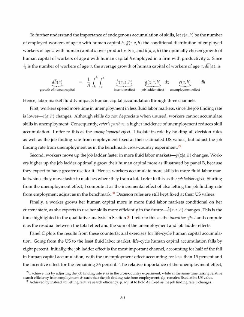
To further understand the importance of endogenous accumulation of skills, let e(a, h) be the number

of employed workers of age a with human capital h, g(z|a, h) the conditional distribution of employed

workers of age a with human capital h over productivity z, and h(a, z, h) the optimally chosen growth of

human capital of workers of age a with human capital h employed in a firm with productivity z. Since1A is the number of workers of age a, the average growth of human capital of workers of age a, dh(a), is

dh(a)︸ ︷︷ ︸growth of human capital

=1A

ˆ h

h

ˆ z

zh(a, z, h)︸ ︷︷ ︸

incentive effect

g(z|a, h)︸ ︷︷ ︸job ladder effect

dz e(a, h)︸ ︷︷ ︸unemployment effect

dh

Hence, labor market fluidity impacts human capital accumulation through three channels.

First, workers spend more time in unemployment in less fluid labor markets, since the job finding rate

is lower—e(a, h) changes. Although skills do not depreciate when unused, workers cannot accumulate

skills in unemployment. Consequently, ceteris paribus, a higher incidence of unemployment reduces skill

accumulation. I refer to this as the unemployment effect. I isolate its role by holding all decision rules

as well as the job finding rate from employment fixed at their estimated US values, but adjust the job

finding rate from unemployment as in the benchmark cross-country experiment.29

Second, workers move up the job ladder faster in more fluid labor markets—g(z|a, h) changes. Work-

ers higher up the job ladder optimally grow their human capital more as illustrated by panel B, because

they expect to have greater use for it. Hence, workers accumulate more skills in more fluid labor mar-

kets, since they move faster to matches where they train a lot. I refer to this as the job ladder effect. Starting

from the unemployment effect, I compute it as the incremental effect of also letting the job finding rate

from employment adjust as in the benchmark.30 Decision rules are still kept fixed at their US values.

Finally, a worker grows her human capital more in more fluid labor markets conditional on her

current state, as she expects to use her skills more efficiently in the future—h(a, z, h) changes. This is the

force highlighted in the qualitative analysis in Section 3. I refer to this as the incentive effect and compute

it as the residual between the total effect and the sum of the unemployment and job ladder effects.

Panel C plots the results from these counterfactual exercises for life-cycle human capital accumula-

tion. Going from the US to the least fluid labor market, life-cycle human capital accumulation falls by

eight percent. Initially, the job ladder effect is the most important channel, accounting for half of the fall

in human capital accumulation, with the unemployment effect accounting for less than 15 percent and

the incentive effect for the remaining 36 percent. The relative importance of the unemployment effect,

29I achieve this by adjusting the job finding rate p as in the cross-country experiment, while at the same time raising relativesearch efficiency from employment, φ, such that the job finding rate from employment, φp, remains fixed at its US value.

30Achieved by instead not letting relative search efficiency, φ, adjust to hold φp fixed as the job finding rate p changes.

30

FIGURE 10. UNDERSTANDING THE INTERACTION BETWEEN TRAINING AND FLUIDITY

(A) WAGE GROWTH (B) OPTIMAL GROWTH RATE (C) HUMAN CAPITAL

Note: Panel A. Decomposition of the effect of labor market fluidity on life-cycle wage growth based on (14). Panel B. Unemployment effect:Counterfactual impact of labor market fluidity holding decision rules and all flows fixed at their US values apart from the job finding ratefrom unemployment, which evolves as in the benchmark cross-country experiment. Job ladder effect: Incremental counterfactual impact oflabor market fluidity of also letting the JJ mobility rate evolve as in the benchmark cross-country experiment, but still under decision rulesfixed at their US values. Incentive effect: Incremental effect of also letting decision rules adjust as in the benchmark cross-country experiment,computed as the difference between the total effect and the combined unemployment and job ladder effects. Source: Model.

however, rises as labor market fluidity falls further relative to the US, rising to 41 percent in the least

fluid labor market. Correspondingly, the relative importance of the job ladder effect falls to 35 percent

and the incentive effect to 24 percent for the least fluid labor market.

One interpretation of this key finding is that the most important channel through which labor mar-

ket fluidity impacts human capital accumulation is backward-looking, as opposed to forward-looking.

Greater labor market fluidity lets workers faster locate jobs where they have greater use for their skills

and where they consequently optimally accumulate more skills. This includes leaving unemployment

faster. In contrast, faster expected future growth in match productivity plays a non-trivial, yet quanti-

tatively less important role.31 To the extent that human capital accumulation is exogenous but workers

cannot accumulate skills when unemployed, the unemployment effect would still be operative. In this

scenario, human capital would grow by four percent more in the US relative to the least fluid labor mar-

ket. Alternatively, suppose that human capital accumulation remained unaffected by changes in labor

market fluidity, but still varied in the cross-section across the job ladder as in the estimated model. In

this case, also the job ladder effect would be at work, such that human capital accumulation would be

seven log points greater in the US relative to the least fluid labor market.

Instead of holding human capital accumulation fixed across countries, an alternative counter-factual

would be to assume that it plays no role in life-cycle wage growth. Indeed, I find in a model recalibrated

to load all life-cycle wage growth in the US on the job ladder that cross-country differences in labor

31For this reason, the impact of labor market fluidity on human capital accumulation is not very sensitive to workers’ bargain-ing power, as I discuss further in Appendix D.5. Workers’ bargaining power primarily impacts training through the incentiveeffect, and this effect only accounts for a quarter to a third of the overall impact of fluidity on human capital accumulation.

31

market fluidity account for a similar share of differences in life-cycle wage growth and aggregate labor

productivity as in the benchmark model. I stress, however, that the estimated model nests this possibility

(µ → 0), but my estimates reject this scenario. Instead, the estimates imply that human capital accumu-

lation does play an important role in life-cycle wage growth. For this reason, I view this alternative

counter-factual as less relevant, and abstract from discussing it further in the interest of space.

4.5 An alternative policy experiment

The analysis above introduced wedges to firms’ cost of job creation, targeted to match cross-country dif-

ferences in labor market fluidity. This approach is motivated by a long literature that argues that various

policies serve to raise the cost on firms of hiring (Hopenhayn and Rogerson, 1993), as well as observable

differences in the cost to firms of doing business (see Section 6). That being said, an alternative approach

to matching differences in labor market fluidity would be to introduce differences in the relative inten-

sity of search on the job, φ. Figure 11 instead varies φ to match cross-country differences in labor market

fluidity, while holding the job finding rate p fixed at its US level.32 I label this alternative experiment the

JJ effect, since it isolates the role of moving up the job ladder. I compute the importance of variation in p

only—the UE effect—as the residual between the overall effect and the impact of varying φ only.

Panel A shows that a slower rate of climbing the job ladder accounts for 92 percent of the slower

life-cycle growth in wages in less fluid labor markets, while Panel B finds that it accounts for 60 percent

of the lower accumulation of human capital. It reduces human capital accumulation both by slowing

down workers’ reallocation up the job ladder to jobs where they train a lot and by discouraging training

conditional on place in the job ladder, since workers expect to have less use for their skills in the future.

While this alternative interpretation of cross-country differences in labor market fluidity does not allow

the model to also match the higher UE rate in more fluid labor markets (see Appendix D), I conclude

that the main predictions carry through (although they are somewhat moderated).

5 Confronting the theory with training data

The theory makes rich predictions for how training varies both across and within countries. In this

section, I confront the predictions of the model with cross-country micro data on training. To that end, I

32Note that because the job finding rate p is an equilibrium object, this requires varying the cost of job creation c in thebackground. I prefer this approach of holding p fixed, since it isolates the importance of variation in φ only. Because workersstill move away from low productive jobs with a higher chance of breaking up at a slower rate when the search intensity fromemployment, φ, is lower, the incidence of unemployment remains higher in low-φ countries. Nevertheless, over 90 percentof unemployment differences disappear once differences in the job finding rate from unemployment are shut down, such thatremaining differences in the incidence of unemployment play a second-order role in driving results.

32

FIGURE 11. THE ROLE OF A HIGHER RATE OF CLIMBING THE JOB LADDER

(A) WAGE GROWTH (B) HUMAN CAPITAL ACCUMULATION

Note: JJ: Counterfactual effect of only letting the job finding rate from employment adjust as in the benchmark cross-country experiment,holding fixed the job finding rate from unemployment, p, at its US value, computed by varying relative search efficiency of the employed, φ,to match the cross-country variation in labor market fluidity. UE: Counterfactual effect of only letting the job finding rate from unemploymentadjust as in the benchmark cross-country experiment, holding fixed the job finding rate from employment, computed as the difference betweenthe total effect and the JJ effect. Source: Model.

exploit the ECHP, which records days and hours spent on on-the-job training, who paid for the training,

etc. A key advantage of the ECHP is that it was conducted by the statistical agency of the EU using a

common questionnaire and processing routines, facilitating the cross-country comparison. This limits

concerns about comparability in cross-country studies of training (Acemoglu and Pischke, 1999a).

5.1 Aggregate patterns

Panel A of Table 5 regresses days or hours on training in the past 12 months, expressed as a fraction

of total work days/hours (5*52 or 40*52, respectively), on labor market fluidity at the country-level.33

The "Raw" column includes only year controls. Workers train more in more fluid labor markets. The

"Controls" column adds controls for worker observable characteristics, including age, education, one-

digit occupation and one-digit sector. While older workers train less and college graduates train more,

controlling for compositional differences does not change the main takeaway of a positive correlation

between labor market fluidity and time on training. The "Direct" column also controls for whether the

worker made a JJ move in the past year. There is no statistical correlation between training and JJ mobility

in the past year. Hence, the positive correlation between labor market fluidity and training is not due to

33The reported time in training is since January in the year prior to the survey. If the training started more than 12 monthsprior to the survey date, I use reported start dates of training to adjust training to a per-past-12-months basis (i.e. if the workerreports 20 training days since January last year, her survey was conducted in April and she reports starting training in Februarylast year, my measure of training days is 12/14 ∗ 20). I top-code the training measures at 13 weeks of full time training per year.This concerns 1.5 percent of observations. Results without top-coding in Appendix E.1 are more pronounced.

33

a mechanical effect of new hires being trained to perform the required tasks of the new job.34

The "Model" column repeats the exercise in the model. I simulate a monthly approximation of the

model and aggregate it to yearly data such that employer outcomes are recorded in "May" every year,

while annual training is the sum of i(a, z, h) over the 12 months prior to the "survey," and the wage is the

average wage over the past "calendar year." I simulate several "countries" that span the relevant range for

labor market fluidity, and implement the same regression as in the data on the pooled model-generated

data. The mechanism emphasized in this paper accounts for a large share of the systematically higher

level of training in more fluid labor markets, somewhat understating the empirical relationship.

Panel B instead exploits within-country variation across education groups (less than college and col-

lege or more), occupations (10 one-digit occupations), or sectors (12 one-digit sectors). I compute labor

market fluidity in the same way as above, but separately by education groups/occupation/sector and

country, and relate this to hours on training in the past 12 months, expressed as a fraction of total work

hours (40*52). In order to reduce somewhat the wide standard errors, I expand the sample to include

all men aged 18–64. The "Baseline" column shows results with country and year fixed effects. Workers

spend more time on training in more fluid education groups/occupations/sectors, although the stan-

dard errors are much larger than in the cross-country specification such that not all point estimates are

statistically significant. The "FE" column adds also education group/occupation/sector fixed effects, i.e.

it exploits the fact that, for instance, college graduates may be particularly fluid and train disproportion-

ately much in some country, relative to average fluidity and training in that country as well as average

fluidity and training of college graduates across all countries. Workers spend more time on training

when their education group/occupation/sector is more fluid relative to the rest of their country as well

as the same education group/occupation/sector in other countries, although not all point estimates are

statistically significant. I also repeat the model estimates from the cross-country simulated data, which

is valid under the strong assumption that education group/occupation/sector is a permanent trait of

workers and labor markets are perfectly segmented by such traits. I conclude that both the across and

within-country variation is supportive of the hypothesis in this paper, also quantitatively.

Appendix E.3 shows that over 70 percent of workers report that their employer paid for their training

(if anything, the share rises with labor market fluidity but the pattern is not statistically significant). At

the same time, it is not clear whether a respondent correctly perceives who paid for the training. In fact,

Appendix B.1 finds that workers earn lower wages during periods when they train more, conditional on

34The ECHP also records whether a reason for taking the course was to improve the respondent’s skills or job prospects.On average across countries, 93 percent of respondents answer yes to this question and there is no meaningful cross-countrycorrelation between the share who answer yes and fluidity. For this reason, I do not further analyze responses to this question.

34

TABLE 5. TRAINING AND LABOR MARKET FLUIDITY

Panel A. Cross-country correlation

Days on training (fraction of year) Hours on training (fraction of year) ModelRaw Controls Direct Raw Controls Direct

Fluidity 0.448*** 0.386*** 0.388*** 0.360*** 0.305*** 0.312*** 0.277***(0.091) (0.083) (0.066) (0.050) (0.038) (0.031) (0.009)

JJ 0.000 0.001(0.002) (0.001)

Age -0.000*** -0.000*** -0.000*** -0.000***(0.000) (0.000) (0.000) (0.000)

College 0.006*** 0.007*** 0.003*** 0.004***(0.002) (0.002) (0.001) (0.001)

N 135,563 115,897 63,634 135,318 115,676 63,494 3,990,963

Panel B. Within-country correlation (hours as fraction of year)

Education Occupation Sector ModelBaseline FE Baseline FE Baseline FE

Fluidity 0.305 0.380 0.317 0.458** 0.328*** 0.419*** 0.277***(0.836) (0.822) (0.226) (0.222) (0.079) (0.096) (0.009)

N 204,207 204,207 148,155 148,155 148,782 148,782 3,990,963

Note: Panel A: Men aged 25–54. Regression of training outcome on labor market fluidity at the country-level, with or without controls. Raw:Controls for year. Controls: Controls for age, education, occupation, sector and year. Direct: Controls for age, education, occupation, sector,year and JJ mobility in previous year. Data: Days or hours on vocational training in the past 12 months, expressed as a fraction of potential workdays/hours (5*52 or 40*52, respectively). Hours and days on training are top-coded at 13 weeks of full time training per year. Model: Fractionof time devoted to training, i(a, h, z). Regressions are weighted using the provided survey weights, renormalized to give each country thesame aggregate weight. Standard errors are clustered at the country level. Panel B. Men aged 18–64. Regression of training outcome on labormarket fluidity at the country-education group/occupation/sector level. Baseline includes country and year fixed effects; FE includes country,year and education group/occupation/sector fixed effects. Data: Hours on vocational training in the past 12 months, expressed as a fractionof potential work hours (40*52). Model: Fraction of time devoted to training, i(a, h, z). Regressions are weighted using the provided surveyweights, renormalized to give each country-education group/occupation/sector the same aggregate weight. Standard errors are clustered atthe country-education group/occupation/sector-year level. Labor market fluidity: Share of employees who started working for their currentemployer at some point in the past 11 months while having been employed in all of the past 12 months. Employment in the past 12 monthsincludes self-employment. ** statistically significant at 5%; *** statistically significant at 1%. Source: ECHP 1995–2001 and model.

worker fixed effects and time-varying observables, consistent with workers sharing the cost of training

(this pattern is true even among those who report that their employer paid for the training). Appendix

E.4 finds no statistically significant correlation between vocational training in the previous year and

current JJ mobility. That is, workers who train more are not more likely to remain with their current

employer, in contrast to what one may have hypothesized if skills were firm-specific.

5.2 Disaggregate patterns

The theory also makes rich predictions for how training varies in the cross-section. As highlighted by

Figure 10, workers grow their human capital less when employed in less productive firms, as they have

less use for it. In more fluid labor markets, however, workers currently in low productive firms expect

to be able to move away from such firms faster. Consequently, while workers in general train less in

35

less productive firms, in a relative sense they train more in low productive firms in more fluid labor

markets. In contrast, absent separation shocks, training at the top of the job ladder is unaffected by

labor market fluidity. Separation shocks moderate this prediction, but the intuition remains: training

should be particularly low in less productive firms in less fluid labor markets. By differencing out any

country-specific factors, this may provide a more robust test of the predictions of the model.

Testing this prediction is somewhat complicated by the fact that the available data do not contain

productivity. They do, however, report firm size, grouped into size bins 1–4, 5–19, 20–49, 50–99, 100–

499, and 500+ employees. Pooling across countries, these size categories contain close to equal shares of

employment. Under the assumption of a monotone relationship between productivity and size, the six

size bins allow me to group firms into (roughly) employment-weighted productivity sextiles. I similarly

bin firms based on productivity into employment-weighted sextiles in the model. As an alternative

ranking of firms, I compute firm pay by regressing log wages on indicators for the sextiles—controlling

for age, education, occupation and country-year fixed effects (age and country fixed effects in the model),

wit =6

∑s=1

αssextilesit + Xitβ + ε it (15)

where sextilesit takes value one if worker i in year t works for an employer in sextile s. My measure of firm

pay, f wageit, is the estimated coefficients, {αs}. Appendix E.5 shows the results from (15), highlighting

that larger firms pay better. Firm pay has a standard deviation of 0.114 in the data and 0.123 in the model.

I subsequently regress hours on training in the past 12 months on either firm productivity sextile or firm

pay, xit, as well as its linear interaction with fluidity, controlling for worker-fixed effects and age,

trainingit = α0xit + α1xit × f luidityc + Ii + Xitβ + ε it

The results in Table 6 offer two main takeaways. First, controlling for worker-fixed effects, workers

train more when employed at high-paying, productive (large) firms, consistent with evidence in other

data sets (Arellano-Bover, 2020). The reason is that workers have greater use for their skills in more

productive firms, and as a consequence train more. In contrast, as I discuss further in Appendix E.6, if

the production function had not featured a complementarity between productivity and human capital,

one may expect training to decline in productivity (and hence firm pay). Moreover, as highlighted by

Figure 4, a larger share of workers are employed at high-paying, productive (large) employers in more

fluid labor markets, where ceteris paribus they train more. In fact, as shown in Appendix E.7, the model

matches this pattern fairly well. These findings relate to the job ladder effect discussed in Section 4.4.

36

Second, workers in low fluidity countries particularly train less when employed at low paying, un-

productive (small) firms. The reason is that a worker currently in a low productive firm is particularly

stuck with her current employer in a low fluidity country, where she has less use for her human capi-

tal. She responds by training less. This relates to the incentive effect discussed in Section 4.4. Finally,

recall from Figure 9 that the mechanism also matches well the higher unemployment rate in less fluid la-

bor markets—the unemployment effect in Section 4.4. I conclude that these aggregate and disaggregate

patterns for training lend empirical support for the key predictions of the theory.

TABLE 6. TRAINING IN THE CROSS-SECTION

Data Model

Prod. Wage Prod. Wage

α0 0.002** 0.035** 0.006*** 0.090***(0.001) (0.013) (0.000) (0.003)

α1 -0.028* -0.515** -0.034*** -0.480***(0.012) (0.211) (0.002) (0.034)

N 77,386 77,386 3,990,963 3,990,963

Note: Men aged 25–54. Training on firm productivity sextile / firm wage, as well as its interaction with fluidity. Panel A. Hours on training,top-coded at 13 full-time weeks per year. Firm productivity sextile and firm wage imputed based on size. Panel B. i(a, z, h). Firm wage imputedbased on productivity. Labor market fluidity: Share of employees who started working for their current employer at some point in the past 11months while having been employed in all of the past 12 months. Employment in the past 12 months includes self-employment. Constructedby first collapsing the data to the country-age-year level using the provided survey weights, then to the country level. Standard errors areclustered at the country-level. * statistically significant at 10%; ** statistically significant at 5%; *** statistically significant at 1%. Source: ECHP1995–2001 and model.

6 Labor market fluidity and policy

Inspired by Hsieh and Klenow (2009), the analysis above adopted a wedge approach to cross-country

differences in labor market fluidity in order to focus on the dynamic implications of such differences for

workers’ optimal behavior. I provide in this section a discussion of some prominent potential factors

behind differences in fluidity, building on an extensive literature (Restuccia and Rogerson, 2017).

6.1 Cross-country analysis

Panel A of Figure 12 shows that labor market fluidity is negatively correlated with the World Bank’s

ease of doing business index, consistent with the argument in Fonseca et al. (2001) that such factors

are more important than unemployment benefits and EPL in accounting for cross-country differences

in job creation. Panel B plots the cost of starting a firm relative to GNI per capita, as estimated by the

World Bank. I construct a model counterpart as the cost of creating a job, c, relative to output per capita.

37

FIGURE 12. DETERMINANTS OF LABOR MARKET FLUIDITY

(A) DOING BUSINESS INDEX (B) COST OF STARTING BUSINESS

Note: Male employees aged 25–54. Panel A. Doing business score. Panel B. Data: Cost of starting a firm relative to GNI per capita. Model:Cost of vacancy, c, relative to total output. Model moments are normalized to match the empirical value for the US by first dividing all countryoutcomes in the model by the model outcome for the US and then multiplying all country outcomes by the data outcome for the US. Labormarket fluidity: Share of employees who started working for their current employer at some point in the past 11 months while having beenemployed in all of the past 12 months. Employment in the past 12 months includes self-employment. Constructed by first collapsing the datato the country-age-year level using the provided survey weights, then to the country level. Source: BHPS, ECHP, EUSILC, GSOEP, OECD, PSIDand World Bank 1991–2015.

As the levels are non-comparable, I normalize the model measure to the empirical measure for the US.

Although it only captures the cost of starting a new firm, it is well-known that young firms contribute

a disproportionate share of total job creation. The required wedges are quantitatively consistent with

observed dispersion in the cost of creating jobs across countries.

6.2 Within-country analysis

I next turn to within-country variation in labor market policy. In particular, I exploit a significant reduc-

tion in EPL in Spain in 1994–1995, which overlaps with the years for which I have training data. Panel A

of Figure 13 illustrates the corresponding fall in the OECD’s EPL index in Spain over this period. Spain

went from having the most stringent EPL in my sample to one of the lowest levels among continental

European countries (see Bentolila et al., 2008, for a further discussion of these reforms). Panel B shows

that labor market fluidity rose substantially after the reforms, although with some delay.

Table 7 contrasts the empirical change in entry wages, life-cycle wage growth and on-the-job training

between a pre and post reform period with the predictions of the model. In the data, I compare the wage

profiles of cohorts of workers who entered the labor market before 1995 to those who entered in 1995

or later (labor market entry is measured as when a worker turned 23), and regress log wages on age

dummies restricted to not grow after age 50, fully flexible year effects, a dummy for whether the worker

38

FIGURE 13. CHANGES IN EPL AND LABOR MARKET FLUIDITY IN SPAIN, 1993–2005

(A) EPL (B) LABOR MARKET FLUIDITY

Note: Male employees aged 25–54. Panel A. OECD EPL index. Panel B. Share of employees who started working for their current employer atsome point in the past 11 months while having been employed in all of the past 12 months. Employment in the past 12 months includes self-employment. Constructed by first collapsing the data to the country-age-year level using the provided survey weights, then to the country-yearlevel. Source: ECHP, EUSILC, and OECD 1993–2005.

entered the labor market after the reforms as well as its interaction with a linear in age,

wit = Ait + Yt + Dt + βDt × ait + ε it (16)

In the model, I compare a low-fluidity pre-reform steady-state to a high-fluidity post-reform steady-

state, and implement regression (16) on pooled pre and post reform simulations. For training outcomes,

I compare the years prior to the reform to those after the reforms. I stress that this methodology imposes

several strong assumptions, including that cohorts that entered the labor market before the reforms were

unaffected, while cohorts that entered after expected the change to be permanent.

TABLE 7. A 1994–1995 SPANISH REFORM TO EPL

Panel A. Pre-reform Panel B. Post-reform Panel C. Change (%)

Data Model Data Model Data Model

Annual JJ mobility rate 0.040 0.040 0.075 0.076 87.4% 87.4%Wage at age 23 (log) -0.055 -0.038Wage at age 35 (log) 0.024 0.031Wage at age 50 (log) 0.122 0.117Training, fraction of year 0.008 0.050 0.014 0.067 69.4% 33.9%

Note: Men aged 23–55. Wage profiles are based on a regression of log wages on a full set of age effects as well as a separate age intercept andlinear slope for the cohorts entering the labor market after the reforms (turning 23 in or after year 1995). Wages for different ages are imputedbased on the intercept and linear slope based on regression (16). Model and data moments are constructed identically. Labor market fluidity:Share of employees who started working for their current employer at some point in the past 11 months while having been employed in all ofthe past 12 months. Data: Employment in the past 12 months includes self-employment due to data limitations. Constructed by first collapsingthe data to the country-age-year level using the survey weights, then to the country-period level. Source: ECHP, EUSILC, and model 1993–2015.

39

Wages of labor market entrants fell by 5.5 log points after the reforms in the data. According to

the model, 3.8 log points is due to the rise in labor market fluidity. The fall in entry wages happens

as workers share in the cost of higher training through lower wages. Wages subsequently grow faster,

such that at age 35 they are 2.4 log points higher in the data versus 3.1 log points in the model. At age

50, they are 12 log points higher in the data and model. Although the magnitude of the change in the

policy varies across the two experiments, these results mirror recent findings from a 2001 reduction in

EPL in Italy (Daruich et al., 2020). These authors show that earnings of labor market entrants fell by five

percent after the reform and did not converge to zero until seven years after entry. Finally, the incidence

of training rises significantly after the reforms, in both the model and data.

7 Conclusions

This paper establishes a series of novel findings on cross-country differences in life-cycle careers using

comparable cross-country panel micro data from 23 OECD countries. In particular, wages grow more

over the life-cycle in labor markets where JJ mobility is more common. To understand these patterns

and assess their aggregate economic implications, I propose and estimate a rich theory of labor market

search and endogenous accumulation of skills on the job. The theory predicts that if workers are able

to faster locate jobs where they can better use their skills, it encourages accumulation of skills. Quanti-

tatively, I find that this mechanism accounts for half of the steeper life-cycle wage growth in more fluid

labor markets. Moreover, labor productivity is nine percent lower across the OECD relative to the US.

More broadly, my findings highlight that the dynamic consequences of misallocation can be large. They

deserve more attention in future work.

References

Abowd, John M and Arnold Zellner, “Estimating gross labor-force flows,” Journal of Business & EconomicStatistics, 1985, 3 (3), 254–283.

Acemoglu, Daron, “Training and Innovation in an Imperfect Labour Market,” The Review of EconomicStudies, 1997, 64 (3), 445–464.and Jorn-Steffen Pischke, “Why Do Firms Train? Theory and Evidence,” The Quarterly Journal of

Economics, 1998, 113 (1), 79–119.and Jörn Steffen Pischke, “Beyond becker: Training in imperfect labour markets,” Economic Journal,

1999, 109 (453), 112–142.and Jorn-Steffen Pischke, “The Structure of Wages and Investment in General Training,” Journal of

Political Economy, 1999, 107 (3), 539–572.Arellano-Bover, Jaime, “Consequences of Firm Heterogeneity for Young Workers: First Job and Firm

Size Career,” 2020.Bagger, By Jesper, François Fontaine, Fabien Postel-vinay, and Jean marc Robin, “Tenure, Experience,

Human Capital, and Wages,” American Economic Review, 2014, 104 (6), 1551–1596.Barlevy, Gadi, “The Sullying Effect of Recessions,” Review of Economic Studies, 2002, 69 (1), 65–96.

40

Becker, Gary S., “Investment in Human Capital: A Theoretical Analysis,” Journal of Political Economy,1962, 70 (5), 9–49.

Ben-Porath, Yoram, “The Production of Human Capital and the Life Cycle of Earnings,” Journal of Polit-ical Economy, 1967, 75 (4), 352–365.

Bentolila, Samuel and Giuseppe Bertola, “Firing Costs and Labour Demand: How Bad is Eurosclero-sis?,” The Review of Economic Studies, 1990, 57 (3), 381., Juan J. Dolado, and Juan F. Jimeno, “Two-tier employment protection reforms: The Spanish experi-ence,” 2008.

Bick, Alexander, Nicola Fuchs-Schündeln, and David Lagakos, “How Do Hours Worked Vary withIncome? Cross-Country Evidence and Implications,” American Economic Review, 2018, 108 (1), 170–199.

Bowlus, Audra J and Huju Liu, “The contributions of search and human capital to earnings growth overthe life cycle,” European Economic Review, 2013, 64, 305–331.

Burdett, Kenneth and Dale T Mortensen, “Wage Differentials, Employer Size, and Unemployment,”International Economic Review, 1998, 39 (2), 257–273., Carlos Carrillo-Tudela, and Melvyn Coles, “The Cost of Job Loss,” Review of Economic Studies, 2020,87 (4), 1757–1798., , and Melvyn G. Coles, “Human capital accumulation and labor market equilibrium,” InternationalEconomic Review, 2011, 52 (3), 657–677.

Cahuc, Pierre, Fabien Postel-Vinay, and Jean-Marc Robin, “Wage Bargaining with On-the-Job Search:Theory and Evidence,” 2006.

Daruich, Diego, Sabrina Di Addario, and Raffaele Saggio, “The Effects of Partial Employment Protec-tion Reforms: Evidence from Italy,” 2020.

Dey, Matthew S and Christopher J Flinn, “An Equilibrium Model of Health Insurance Provision andWage Determination,” Econometrica, 2005, 73 (2), 571–627.

Diamond, Peter A, “Aggregate Demand Management in Search Equilibrium,” Journal of Political Econ-omy, 1982, 90 (5), 881–894.

Doepke, Matthias and Ruben Gaetani, “Why Didn’t the College Premium Rise Everywhere? Employ-ment Protection and On-the-Job Investment in Skills,” 2020.

Donovan, Kevin, Will Jianyu Lu, and Todd Schoellman, “Labor Market Dynamics and Development,”2020.

Engbom, Niklas, “Misallocative Growth,” 2020.Feng, Ying, David Lagakos, and James E Rauch, “Unemployment and development,” 2020.Flinn, Christopher, Ahu Gemici, and Steven Laufer, “Search, matching and training,” Review of Eco-

nomic Dynamics, 2017, 25, 260–297.Fonseca, Raquel, Paloma Lopez-Garcia, and Christopher A. Pissarides, “Entrepreneurship, start-up

costs and employment,” European Economic Review, 2001, 45 (4-6), 692–705.Fu, Chao, “Training, search and wage dispersion,” Review of Economic Dynamics, 2011, 14 (4), 650–666.Gervais, Martin, Nir Jaimovich, Henry E. Siu, and Yaniv Yedid-Levi, “What should I be when I grow

up? Occupations and unemployment over the life cycle,” Journal of Monetary Economics, 2016, 83, 54–70.

Gourieroux, C., A. Monfort, and E. Renault, “Indirect inference,” Journal of Applied Econometrics, 1993, 8(1 S), S85–S118.

Gregory, Victoria, “Firms as Learning Environments: Implications for Earnings Dynamics and JobSearch,” 2019.

Griliches, Zvi, “Capital-Skill Complementarity,” The Review of Economics and Statistics, 1969, 51 (4), 465–468.

Guner, Nezih, Andrii Parkhomenko, and Gustavo Ventura, “Managers and productivity differences,”Review of Economic Dynamics, 2018, 29, 256–282.

Guvenen, Fatih, Burhanettin Kuruscu, and Serdar Ozkan, “Taxation of human capital and wage in-equality: A cross-country analysis,” Review of Economic Studies, 2013, 81 (2), 818–850.

Heathcote, Jonathan, Fabrizio Perri, and Giovanni L. Violante, “Unequal we stand: An empirical anal-ysis of economic inequality in the United States, 1967-2006,” Review of Economic Dynamics, 2010, 13 (1),15–51.

41

Heckman, James J, Lance Lochner, and Christopher Taber, “Explaining Rising Wage Inequality: Explo-rations with a Dynamic General Equilibrium Model of Labor Earnings with Heterogeneous Agents,”Review of Economic Dynamics, 1998, 1 (1), 1–58.

Herkenhoff, Kyle, Jeremy Lise, Guido Menzio, and Gordon M Phillips, “Production and Learning inTeams,” 2018.

Hobijn, Bart and Aysegul Sahin, “Job-finding and separation rates in the OECD,” Economics Letters,2009, 104 (3), 107–111.

Hopenhayn, Hugo and Richard Rogerson, “Job Turnover and Policy Evaluation: A General EquilibriumAnalysis,” Journal of Political Economy, oct 1993, 101 (5), 915–938.

Hornstein, Andreas, Per Krusell, and Giovanni L Violante, “Frictional wage dispersion in search mod-els: A quantitative assessment,” American Economic Review, 2011, 101 (7), 2873–2898.

Hsieh, Chang-Tai and Peter J. Klenow, “Misallocation and Manufacturing TFP in China and India,”Quarterly Journal of Economics, 2009, 124 (4), 1403–1448.

Huggett, Mark, Gustavo Ventura, and Amir Yaron, “Sources of lifetime inequality,” American EconomicReview, 2011, 101 (7), 2923–2954.

Jolivet, Grégory, Fabien Postel-Vinay, and Jean Marc Robin, “The empirical content of the job searchmodel: Labor mobility and wage distributions in Europe and the US,” European Economic Review, 2006,50 (4), 877–907.

Jovanovic, Boyan and Yaw Nyarko, “Learning by Doing and the Choice of Technology,” Journal of Polit-ical Economy, 1996, 64 (6), 1299–1310.

Kambourov, Gueorgui and Iourii Manovskii, “Occupational specificity of human capital,” InternationalEconomic Review, 2009, 50 (1), 63–115.

Lagakos, David, Benjamin Moll, Tommaso Porzio, Nancy Qian, and Todd Schoellman, “Life cyclewage growth across countries,” Journal of Political Economy, 2018, 126 (2), 797–849.

Lazear, Edward P., “Job Security Provisions and Employment,” Quarterly Journal of Economics, 1990, 105(3), 699–726.

Lazear, Edward P, “Firm-Specific Human Capital: A Skill-Weights Approach,” Journal of Political Econ-omy, 2009, 117 (5), 914–940.

Lentz, Rasmus and Nicolas Roys, “Training and Search On the Job,” 2016.Ljungqvist, Lars and Thomas J Sargent, “The European Unemployment Dilemma,” Journal of Political

Economy, 1998, 106 (3), 514–550.and Thomas J. Sargent, “Two Questions about European Unemployment,” Econometrica, 2008, 76 (1),1–29.

Manuelli, Rodolfo E. and Ananth Seshadri, “Human capital and the wealth of nations,” American Eco-nomic Review, 2014, 104 (9), 2736–2762.

McCall, John J, “Economics of Information and Job Search,” The Quarterly Journal of Economics, 1970, 84(1), 113–126.

Michelacci, Claudio and Josep Pijoan-Mas, “Intertemporal labour supply with search frictions,” Reviewof Economic Studies, 2012, 79 (3), 899–931.

Mincer, Jacob, Schooling, Experience, and Earnings, New York: NBER Press, 1974.Mortensen, Dale T and Christopher A Pissarides, “Job Creation and Job Destruction in the Theory of

Unemployment,” The Review of Economic Studies, 1994, 61 (3), 397–415.Nickell, Stephen, “Unemployment and Labor Market Rigidities: Europe versus North America,” Journal

of Economic Perspectives, 1997, 11 (3), 55–74.Petrongolo, Barbara and Christopher A. Pissarides, “Looking into the Black Box : A Survey of the

Matching Function,” Journal of Economic Literature,, 2001, 39 (2), 390–431.Poschke, Markus, “Wage Employment, Unemployment and Self-Employment across Countries,” 2019.Poterba, James M and Lawrence H Summers, “Reporting Errors and Labor Market Dynamics,” Econo-

metrica, 1986, 54 (6), 1319–1338.Pries, Michael and Richard Rogerson, “Hiring Policies, Labor Market Institutions, and Labor Market

Flows,” Journal of Political Economy, 2005, 113 (4), 811–839.Restuccia, Diego and Richard Rogerson, “The causes and costs of misallocation,” Journal of Economic

Perspectives, 2017, 31 (3), 151–174.Rosen, Sherwin, “Learning and Experience in the Labor Market,” The Journal of Human Resources, 1972,

7 (3), 326–342.

42

Rubinstein, Ariel, “Perfect Equilibrium in a Bargaining Model,” Econometrica, 1982, 50 (1), 97–109.Rubinstein, Yona and Yoram Weiss, “Post Schooling Wage Growth: Investment, Search and Learning,”

in “Handbook of the Economics of Education,” Vol. 1 2006, pp. 1–67.Topel, Robert H and Michael P Ward, “Job Mobility and the Careers of Young Men,” Quarterly Journal

of Economics, 1992, 107 (2), 439–479.Wasmer, Etienne, “General versus Specific Skills in Labor Markets with Search Frictions and Firing

Costs,” The American Economic Review, 2006, 96 (3), 811–831.Yamaguchi, Shintaro, “Job Search , Bargaining , and Wage Dynamics,” Journal of Labor Economics, 2010,

28 (3), 595–631.

43

Online Appendix—Not for PublicationA Data

This section describes the data sources in some more detail and provides additional empirical results.

A.1 Benchmarking the PSID with the SIPP

The EU rate in the PSID is lower than what researchers typically find in the CPS, but more in line withwhat other research has found in the SIPP (Engbom, 2020). Figure 14 compares the monthly EU andUE rates in the PSID against the SIPP. Broadly, the series compare reasonably well. In particular, boththe PSID and SIPP show significantly lower mobility than, for instance, the CPS. This is consistent withwell-known issues with classification error leading to substantially overstated gross worker flows in theCPS (Abowd and Zellner, 1985; Poterba and Summers, 1986).

FIGURE 14. MONTHLY EU AND UE RATES, PSID VERSUS SIPP

(A) EU

0.0

05.0

1.0

15.0

2M

onth

ly m

obili

ty ra

te

25 30 35 40 45 50 55Age

PSID SIPP

(B) UE0

.1.2

.3.4

Mon

thly

mob

ility

rate

25 30 35 40 45 50 55Age

PSID SIPP

Note: Men 25–54. Panel A. Share of employed workers who are unemployed in the subsequent month. Panel B. Share of unemployed workerswho are employed in the subsequent month. All panels. Employment includes self-employment due to data limitations. Definitions follow ILOstandard. Constructed by first collapsing the data to the country-year-age level using the provided survey weights, then to the country-level.Source: PSID and SIPP 1994–2015.

A.2 Data sources

Table 8 summarizes the annual data set and Table 9 the monthly data set. In total, the annual samplecontains roughly nine hundred thousand individual-years and the monthly sample roughly 11 millionindividual-months. I describe the data sources in some more detail below.

PSID. The PSID has been collected annually since 1968 (biannually since 1997) based on an initiallyrepresentative sample of households and their offspring. Over time, additional households have beenadded, but I focus on the original core sample and their descendants (the so called Survey ResearchCenter sample). Initially, no weights were provided for this sample, since it was representative of the

1

US population. Subsequent attrition and non-response, however, necessitate the use of survey weights,which I employ throughout my analysis. As a large share of the questions in the PSID center around the"head" of the household, I restrict attention to heads of households. Starting in 1988, the PSID asks re-spondents for a monthly calendar of labor market events during the prior calendar year (during the priortwo calendar years starting with the 2003 survey). It also asks for information on up to two employmentspells (in some years more), including start and end dates, earnings, hours, occupation, etc.

GSOEP. The GSOEP was modeled on the PSID and has followed the same individuals annually since1984. Additional samples have been added over time, but I restrict attention to the original, representa-tive samples for West and East Germany. I start the analysis with German reunification in 1991, whichalso corresponds well with the sample period available from the other data sources. I end the analysis in2011 because it was the last year available when I applied for the data several years ago.35 The GSOEPasks a rich set of questions about demographics, income and hours worked, as well as labor force statusin each month during the past calendar year and the start date of the current employment spell. I usesurvey weights throughout my analysis to adjust for nonrandom attrition and non-response.

BHPS. The BHPS began in 1991 and was discontinued in 2008. It is similar to the PSID. The sample hasexpanded over time, but I focus on the original core sample. As the PSID/GSOEP, the BHPS containsdemographic characteristics on the respondent, as well as annual information on gross income and hoursworked. The BHPS also contains information on start and end dates on all labor market spells since thelast survey, which I use to construct a monthly calendar of labor market events as in the PSID/GSOEP. Iuse survey weights throughout my analysis to adjust for nonrandom attrition and non-response.

ECHP. The ECHP was run 1994–2001 across the original set of European Union countries. Because ofconfidentiality restrictions, however, data from Germany and Portugal are not released to researchers.The data from Sweden are only available for a few years and miss several key variables, forcing meto exclude Sweden. Luxembourg switched to collecting data via a separate, national survey after threeyears in the ECHP, dropping several key variables in the process. As the Luxembourg sample for thefirst three years in the ECHP is small, I drop also Luxembourg from my analysis (similar results holdincluding the few available years, though). While data from the UK are available in the ECHP, severalyears are missing so I opt to use the larger and consistently collected BHPS instead. The ECHP followsthe same individuals annually for up to eight years. The survey is similar to the PSID, including a similarset of variables. In particular, it asks for a monthly calendar of events in the prior calendar year and thestart date of the current employment spell. I weigh all results using the provided survey weights.

EUSILC. The EUSILC is the successor to the ECHP starting in 2003. It gradually expanded the set ofcountries covered to eventually include all EU members plus a set of affiliated countries. The surveyis annual and uses a rotating panel design, which differs somewhat in length across countries. Mostcountries follow the same individuals for up to four years, but France follows individuals for eight yearsand Norway for six. As the other surveys, it contains the standard demographic and income variables,including gross annual labor income and hours worked during the previous calendar year. It also con-tains a monthly calendar of labor market events for the prior calendar year. It differs slightly from theother surveys in that it does not contain the start date of the current employment spell, instead recordingwhether the individual switched employer in the past 12 months. All results use survey weights.

35I am awaiting an extension of my project to add the last few years from the GSOEP as well as the EUSILC.

2

TABLE 8. OVERVIEW OF ANNUAL DATA SET

Source Years T NT N

Panel A. Core Western European countries plus the US

Austria ECHP/EUSILC 1995–2014 18 39,700 13,276Belgium ECHP/EUSILC 1994–2014 19 36,070 12,849Denmark ECHP/EUSILC 1994–2013 18 25,883 8,901Finland ECHP/EUSILC 1996–2014 16 48,432 17,867France ECHP/EUSILC 1994–2014 16 58,981 15,951Germany GSOEP 1991–2011 21 60,346 6,640Greece ECHP/EUSILC 1994–2014 15 36,341 12,425Ireland ECHP/EUSILC 1994–2014 17 25,018 8,935Italy ECHP/EUSILC 1994–2014 15 85,926 33,668Netherlands ECHP/EUSILC 1994–2014 18 61,312 21,073Spain ECHP/EUSILC 1994–2014 19 92,355 32,976UK BHPS 1991–2008 18 32,910 4,119US PSID 1994–2015 13 19,047 2,914Total 223 622,321 191,594

Panel B. Other OECD countries

Czech Republic EUSILC 2005–2014 9 27,761 10,805Estonia EUSILC 2004–2014 10 19,682 8,113Hungary EUSILC 2005–2014 10 37,406 16,059Iceland EUSILC 2004–2014 10 10,407 4,522Latvia EUSILC 2007–2014 7 12,684 6,207Lithuania EUSILC 2005–2014 9 13,495 5,414Norway EUSILC 2004–2014 10 22,994 8,241Poland EUSILC 2005–2014 9 46,972 19,850Slovak Republic EUSILC 2005–2013 8 15,404 6,166Slovenia EUSILC 2005–2014 9 47,708 23,487Total 71 221,112 96,101

Note: Men aged 25–54. T: Number of years; NT: Number of individual-years; N: Number of individuals.

SIPP. The SIPP has been conducted in separate panels since the mid-1980s, but a break in the surveyin 1996 implies that data on job-to-job mobility in the earlier panels are not directly comparable to thatin the later panels. To align with the time period covered by the other data sets used by this paper, Ifocus on SIPP data from 1996–2012 (i.e. the 1996, 2001, 2004 and 2008 panels). Each panel of the SIPPfollows a group of individuals over time. Data are collected in "waves", with the respondent in each wavebeing asked to recall labor market events during the prior four months. The survey asks for informationregarding up to four employment spells during the past four months (two as employee and two as self-employed), including start dates and end dates (if applicable), income, hours, occupation, sector, etc. Italso contains standard demographic characteristics. I use the provided survey weights throughout myanalysis to make results representative of the overall US population.

A.3 Life-cycle labor market states

Figure 15 plots the distribution of men across four labor market states—wage employment, self employ-ment, unemployment and non-participation—over the life-cycle, offering three main takeaways. First,workers enter the labor market at a declining pace up to age 30. There is no pronounced covariationbetween age of entry and labor market fluidity, although the US (and somewhat less the UK) appearsto be an outlier. The way the PSID is collected, however, may bias participation rates at young ages if

3

TABLE 9. OVERVIEW OF MONTHLY DATA SET

Source Years T NT N

Panel A. Core Western European countries plus the US

Austria ECHP/EUSILC 1995–2014 214 544,535 15,029Belgium ECHP/EUSILC 1994–2014 225 482,697 14,548Denmark ECHP/EUSILC 1994–2014 213 243,673 6,163Finland ECHP/EUSILC 1996–2014 189 430,234 11,935France ECHP/EUSILC 1994–2014 201 833,033 18,442Germany GSOEP 1991–2011 239 756,609 6,758Greece ECHP/EUSILC 1994–2014 177 491,048 14,198Ireland ECHP/EUSILC 1994–2014 201 342,759 10,175Italy ECHP/EUSILC 1994–2014 177 1,162,774 38,537Netherlands ECHP/EUSILC 1994–2014 213 550,911 14,440Spain ECHP/EUSILC 1994–2014 225 1,247,297 37,304UK BHPS 1991–2014 228 466,563 4,412US PSID 1994–2015 225 374,570 2,978Total 2,727 7,926,703 194,919

Panel B. Other OECD countries

Czech Republic EUSILC 2005–2014 106 387,008 12,714Estonia EUSILC 2004–2014 118 267,939 9,227Hungary EUSILC 2005–2014 118 523,418 18,824Iceland EUSILC 2004–2014 82 95,374 4,198Latvia EUSILC 2007–2014 82 172,982 7,164Lithuania EUSILC 2005–2014 106 191,482 6,337Norway EUSILC 2004–2014 118 225,178 7,227Poland EUSILC 2005–2014 106 651,946 22,992Slovak Republic EUSILC 2005–2013 94 204,716 6,849Slovenia EUSILC 2005–2014 106 646,751 26,696Total 1,036 3,366,794 122,228

Note: Men aged 25–54. T: Number of months; NT: Number of individual-months; N: Number of individuals.

those who participate in the labor market are also more likely to have formed their own households (theSIPP, in contrast, shows an increase in male labor force participation rates between age 20–25). By notfocusing on the head of household like the PSID, the other surveys may be less prone to this.

Second, participation rates remain high and roughly constant until age 50, after which they start todecline. The decline becomes pronounced after around age 55. Third, the share of wage employed fallsgradually after age 30, while the share of self-employed rises. There is also some evidence of a higherself-employment rate in less fluid labor markets. As I show in Appendix D.3, the model is consistentwith this pattern if self-employment is interpreted as out of necessity, i.e. akin to unemployment. Whilethe share of self-employment remains modest across all countries, it would be interesting to develop adeeper theory of this than necessity entrepreneurs in future research (see, for instance, Engbom, 2020,for a joint model of labor market search and entrepreneurship).

Figure 16 plots labor force participation rates for men 25–54, men aged 25 and men aged 54 againstlabor market fluidity. While there is dispersion across countries in participation, it is only weakly corre-lated with labor market fluidity. Figure 17 plots the share of men who are in the labor force in year t butnot in the labor force in year t + 2. I focus on two-year later outcomes to be able to use also the biannualPSID years after 1997. The share remains low up to around age 50, when it starts to gradually rise.

4

FIGURE 15. LIFE-CYCLE LABOR MARKET STATES

(A) AUSTRIA

0.25

.5.75

1Share

20 30 40 50 60Age

(B) BELGIUM

0.25

.5.75

1Share

20 30 40 50 60Age

(C) DENMARK

0.25

.5.75

1Share

20 30 40 50 60Age

(D) FINLAND

0.25

.5.75

1Share

20 30 40 50 60Age

(E) FRANCE0

.25

.5.75

1Share

20 30 40 50 60Age

(F) GERMANY

0.25

.5.75

1Share

20 30 40 50 60Age

(G) GREECE

0.25

.5.75

1Share

20 30 40 50 60Age

(H) IRELAND

0.25

.5.75

1Share

20 30 40 50 60Age

(I) ITALY

0.25

.5.75

1Share

20 30 40 50 60Age

(J) NETHERLANDS

0.25

.5.75

1Share

20 30 40 50 60Age

(K) SPAIN

0.25

.5.75

1Share

20 30 40 50 60Age

(L) UK

0.25

.5.75

1Share

20 30 40 50 60Age

(M) US

0.25

.5.75

1Share

20 30 40 50 60Age

Note: Share of men aged 20–60 by labor market status. Solid black: wage employed. Dash-dotted green: self-employed. Dashed blue: unemployed. Dotted purple: not-in-the laborforce. Labor market states follow ILO standard. All moments: Constructed by first collaps-ing the data to the country-year-age level using the provided survey weights, then to thecountry-level. Source: BHPS, ECHP, EUSILC, GSOEP and PSID 1991–2015.

5

FIGURE 16. LABOR FORCE PARTICIPATION RATES AND LABOR MARKET FLUIDITY

(A) ALL (B) AGE 25

(C) AGE 54

Note: Men aged 25–54. Panel A. Share of all men aged 25–54 that isin the labor force. Panel B. Share of men aged 25 that is in the laborforce. Panel C. Share of men aged 54 that is in the labor force. Allpanels. Labor force includes the wage employed, self-employed andunemployed. Employment status based on ILO standard. Constructedby first collapsing the data to the country-year-age level using the pro-vided survey weights, then to the country level. Labor market fluidity:Share of employees who started working for their current employer atsome point in the past 11 months while having been employed in all ofthe past 12 months. Employment in the past 12 months includes self-employment due to data limitations. Constructed by first collapsing thedata to the country-age-year level using the provided survey weights,then to the country-level. Source: BHPS, ECHP, EUSILC, GSOEP andPSID 1991–2015.

6

FIGURE 17. LABOR FORCE EXIT RATES

(A) AUSTRIA

0.1

.2.3

.4E

xit r

ate

25 35 45 55 65Age

(B) BELGIUM

0.1

.2.3

.4E

xit r

ate

25 35 45 55 65Age

(C) DENMARK

0.1

.2.3

.4E

xit r

ate

25 35 45 55 65Age

(D) FINLAND

0.1

.2.3

.4E

xit r

ate

25 35 45 55 65Age

(E) FRANCE0

.1.2

.3.4

Exi

t rat

e

25 35 45 55 65Age

(F) GERMANY

0.1

.2.3

.4E

xit r

ate

25 35 45 55 65Age

(G) GREECE

0.1

.2.3

.4E

xit r

ate

25 35 45 55 65Age

(H) IRELAND

0.1

.2.3

.4E

xit r

ate

25 35 45 55 65Age

(I) ITALY

0.1

.2.3

.4E

xit r

ate

25 35 45 55 65Age

(J) NETHERLANDS

0.1

.2.3

.4E

xit r

ate

25 35 45 55 65Age

(K) SPAIN

0.1

.2.3

.4E

xit r

ate

25 35 45 55 65Age

(L) UK

0.1

.2.3

.4E

xit r

ate

25 35 45 55 65Age

(M) US

0.1

.2.3

.4E

xit r

ate

25 35 45 55 65Age

Note: Male employees aged 25–63. Share of labor force participants in year t who are not inthe labor force at year t + 2. Employment status is based on ILO standards. Computed byfirst collapsing the data to the age-year-country level using the provided survey weights,then to the country-age-level. Source: BHPS, ECHP, EUSILC, GSOEP and PSID 1991–2015.

7

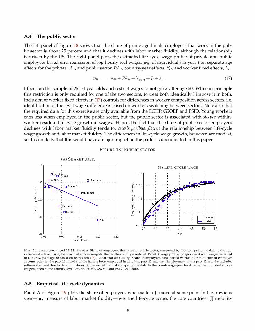
A.4 The public sector

The left panel of Figure 18 shows that the share of prime aged male employees that work in the pub-lic sector is about 25 percent and that it declines with labor market fluidity, although the relationshipis driven by the US. The right panel plots the estimated life-cycle wage profile of private and publicemployees based on a regression of log hourly real wages, wit, of individual i in year t on separate ageeffects for the private, Ait, and public sector, PAit, country-year effects, Yct, and worker fixed effects, Ii,

wit = Ait + PAit + Yc(i)t + Ii + ε it (17)

I focus on the sample of 25–54 year olds and restrict wages to not grow after age 50. While in principlethis restriction is only required for one of the two sectors, to treat both identically I impose it in both.Inclusion of worker fixed effects in (17) controls for differences in worker composition across sectors, i.e.identification of the level wage difference is based on workers switching between sectors. Note also thatthe required data for this exercise are only available from the ECHP, GSOEP and PSID. Young workersearn less when employed in the public sector, but the public sector is associated with steeper within-worker residual life-cycle growth in wages. Hence, the fact that the share of public sector employeesdeclines with labor market fluidity tends to, ceteris paribus, flatten the relationship between life-cyclewage growth and labor market fluidity. The differences in life-cycle wage growth, however, are modest,so it is unlikely that this would have a major impact on the patterns documented in this paper.

FIGURE 18. PUBLIC SECTOR

(A) SHARE PUBLIC

(B) LIFE-CYCLE WAGE

Note: Male employees aged 25–54. Panel A. Share of employees that work in public sector, computed by first collapsing the data to the age-year-country level using the provided survey weights, then to the country-age-level. Panel B. Wage profile for ages 25–54 with wages restrictedto not grow past age 50 based on regression (17). Labor market fluidity: Share of employees who started working for their current employerat some point in the past 11 months while having been employed in all of the past 12 months. Employment in the past 12 months includesself-employment due to data limitations. Constructed by first collapsing the data to the country-age-year level using the provided surveyweights, then to the country-level. Source: ECHP, GSOEP and PSID 1991–2015.

A.5 Empirical life-cycle dynamics

Panal A of Figure 19 plots the share of employees who made a JJ move at some point in the previousyear—my measure of labor market fluidity—over the life-cycle across the core countries. JJ mobility

8

has a common shape: it is high early in careers, and subsequently declines substantially as individualsage. There are significant differences in the level of labor market fluidity across countries, with somecountries displaying higher fluidity at all ages. These high fluidity countries include the Anglo-Saxoncountries (UK and US), as well as Denmark and the Netherlands. On the other end of the spectrum,Belgium, Austria and Greece have JJ mobility rates that are less than half those in the US at all ages.

Panel B plots wage growth between ages 25–50 across countries, assuming that wages do not growafter age 50. Across all countries, life-cycle wage profiles share a common shape, with wages growingrapidly early in careers. In contrast to the common shape, there is a remarkable degree of heterogeneityacross countries in the overall wage growth over the life-cycle, as emphasized by Lagakos et al. (2018).36

FIGURE 19. LABOR MARKET FLUIDITY AND LIFE-CYCLE WAGE GROWTH

(A) JJ MOBILITY (B) WAGE GROWTH

Note: Male employees aged 25–54. JJ mobility: Share of employees who started working for their current employer at some point in the past11 months while having been employed in all of the past 12 months. Employment in the past 12 months includes self-employment due to datalimitations. Constructed by first collapsing the data to the country-age-year level using the provided survey weights, then to the country-age-level. Log hourly real wage profile based on (1) with worker fixed effects, time effects and age effects restricted to not grow past age 50. Source:BHPS, ECHP, EUSILC, GSOEP and PSID 1991–2015.

Panel A of Figure 20 plots the monthly EU rate over the life-cycle across countries. The EU rate sharesa common shape across countries, with high rates of job loss early in careers and subsequent declines.Aggregate cross-country differences are less pronounced than for JJ mobility, with Spain as an exception.Moreover, there is no evidence that high-fluidity countries also have higher EU mobility rates. In fact,the correlation between the aggregate EU rate and labor market fluidity is negative.

Panel B plots the monthly UE rate over the life-cycle across countries. The profiles are noisier than theother mobility rates, because the sample of unemployed is much smaller than the sample of employed.The life-cycle pattern of UE mobility is somewhat more heterogeneous across countries. Most countriesdisplay modest declines in the UE rate over the life-cycle, but a few countries have more pronounceddeclines, while others see increases. There are also significant differences also in the UE rate acrosscountries, and the aggregate UE rate is positively correlated with labor market fluidity.

36Where our studies overlap, my wage profiles align well with Lagakos et al. (2018). The main exception is Germany, whichthey find has the highest wage growth (steeper than the US). I confirm this finding in a specification that includes workers aged22–59, which may be closer to their specifications that include all workers with 0–40 years of experience. My patterns remainrobust to such alternative specifications. Nevertheless, I prefer to focus on ages 25–54 due to higher non-participation ratesprior to 25 and after age 54 (see Appendix A.3), which the theory abstracts from.

9

FIGURE 20. EU AND UE RATES AND LABOR MARKET FLUIDITY

(A) EU RATE (B) UE RATE

Note: Men aged 25–54. EU: Share of employed who are unemployed in the subsequent month. UE: Share of unemployed who are employedin the subsequent month. Employment includes self-employed due to data limitations. Constructed by first collapsing to the country-age-yearlevel using the provided survey weights, then to the country-age level. Source: BHPS, ECHP, EUSILC, GSOEP and PSID 1991–2015.

A.6 The role of composition, full sample

Table 10 replicates the regression results for life-cycle wage growth and labor market fluidity controllingfor compositional differences for the full sample of 23 countries. Results are very similar to the coresample.

TABLE 10. LIFE-CYCLE WAGE GROWTH AND LABOR MARKET FLUIDITY

Panel A. Ages 25–54 Panel B. 1% depreciation Panel C. Ages 22–59

Baseline Educ Occup Baseline Educ Occup Baseline Educ Occup

α 0.242*** 0.217** 0.219** 0.242*** 0.217** 0.219** 0.257*** 0.228*** 0.231***(0.081) (0.083) (0.078) (0.081) (0.083) (0.078) (0.078) (0.078) (0.076)

N 474,919 472,836 449,644 474,919 472,836 449,644 562,239 559,214 531,729

Note: Male employees. Panel A. Wages restricted to not grow after age 50. Panel B. Ages 25–54 with wages restricted to depreciate 1% annuallyafter age 50. Panel C. Wages restricted to not grow after age 50. Labor market fluidity: Share of employees who started working for their currentemployer at some point in the past 11 months while having been employed in all of the past 12 months. Employment in the past 12 monthsincludes self-employment due to data limitations. Constructed by first collapsing the data to the country-age-year level using the providedsurvey weights, then to the country level. α: Fluidity-age interaction in regression (2) with worker fixed effects, time effects and restricted ageeffects. Standard error below are clustered at the country-level. ** statistically significant at 5%; *** statistically significant at 1%. Source: BHPS,ECHP, EUSILC, GSOEP and PSID 1991–2015.

A.7 Raw and residual life-cycle inequality

Figure 21 correlates various measures of inequality and life-cycle growth in inequality with labor marketfluidity. There is possibly some evidence that inequality is higher in more fluid labor markets, whilegrowth in inequality is lower. As it turns out, these patterns are consistent with the predictions of themodel. The patterns, however, are not pronounced (which is also consistent with the theory).

10

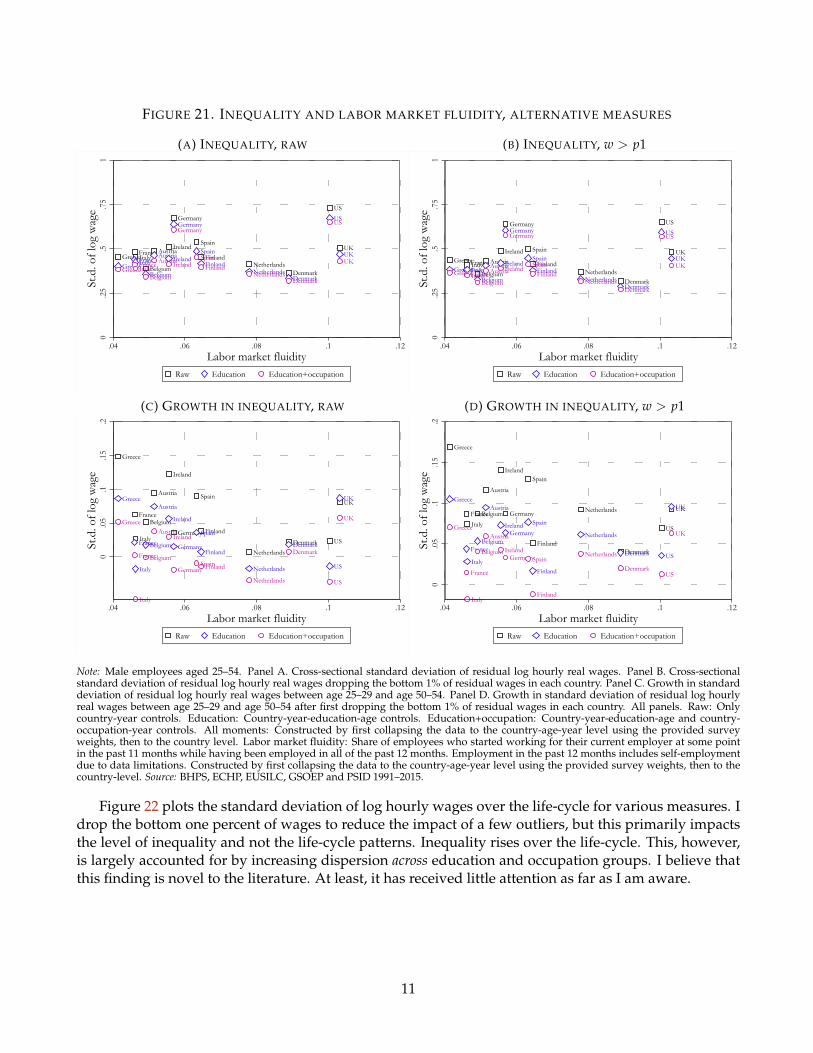
FIGURE 21. INEQUALITY AND LABOR MARKET FLUIDITY, ALTERNATIVE MEASURES

(A) INEQUALITY, RAW

Austria

Belgium Denmark

FinlandFrance

Germany

GreeceIreland

ItalyNetherlands

SpainUK

US

Austria

Belgium Denmark

FinlandFrance

Germany

GreeceIrelandItaly

Netherlands

Spain UK

US

Austria

Belgium Denmark

FinlandFrance

Germany

GreeceIrelandItaly

Netherlands

Spain UK

US

0.2

5.5

.75

1St

.d. o

f log

wag

e

.04 .06 .08 .1 .12Labor market fluidity

Raw Education Education+occupation

(B) INEQUALITY, w > p1

Austria

BelgiumDenmark

FinlandFrance

Germany

GreeceIreland

ItalyNetherlands

Spain UK

US

Austria

BelgiumDenmark

FinlandFrance

Germany

GreeceIreland

ItalyNetherlands

Spain UK

US

Austria

BelgiumDenmark

FinlandFrance

Germany

Greece IrelandItaly

Netherlands

Spain UK

US

0.2

5.5

.75

1St

.d. o

f log

wag

e

.04 .06 .08 .1 .12Labor market fluidity

Raw Education Education+occupation

(C) GROWTH IN INEQUALITY, RAW

Austria

Belgium

Denmark

Finland

France

Germany

Greece

Ireland

Italy

Netherlands

SpainUK

US

Austria

Belgium DenmarkFinland

France Germany

Greece

Ireland

Italy Netherlands

Spain

UK

US

Austria

BelgiumDenmark

Finland

France

Germany

Greece

Ireland

Italy

Netherlands

Spain

UK

US

0.0

5.1

.15

.2St

.d. o

f log

wag

e

.04 .06 .08 .1 .12Labor market fluidity

Raw Education Education+occupation

(D) GROWTH IN INEQUALITY, w > p1

Austria

Belgium

DenmarkFinland

France Germany

Greece

Ireland

Italy

Netherlands

Spain

UK

US

Austria

Belgium

Denmark

Finland

France

Germany

Greece

Ireland

Italy

Netherlands

Spain

UK

US

Austria

Belgium

Denmark

Finland

France

Germany

Greece

Ireland

Italy

NetherlandsSpain

UK

US

0.0

5.1

.15

.2St

.d. o

f log

wag

e

.04 .06 .08 .1 .12Labor market fluidity

Raw Education Education+occupation

Note: Male employees aged 25–54. Panel A. Cross-sectional standard deviation of residual log hourly real wages. Panel B. Cross-sectionalstandard deviation of residual log hourly real wages dropping the bottom 1% of residual wages in each country. Panel C. Growth in standarddeviation of residual log hourly real wages between age 25–29 and age 50–54. Panel D. Growth in standard deviation of residual log hourlyreal wages between age 25–29 and age 50–54 after first dropping the bottom 1% of residual wages in each country. All panels. Raw: Onlycountry-year controls. Education: Country-year-education-age controls. Education+occupation: Country-year-education-age and country-occupation-year controls. All moments: Constructed by first collapsing the data to the country-age-year level using the provided surveyweights, then to the country level. Labor market fluidity: Share of employees who started working for their current employer at some pointin the past 11 months while having been employed in all of the past 12 months. Employment in the past 12 months includes self-employmentdue to data limitations. Constructed by first collapsing the data to the country-age-year level using the provided survey weights, then to thecountry-level. Source: BHPS, ECHP, EUSILC, GSOEP and PSID 1991–2015.

Figure 22 plots the standard deviation of log hourly wages over the life-cycle for various measures. Idrop the bottom one percent of wages to reduce the impact of a few outliers, but this primarily impactsthe level of inequality and not the life-cycle patterns. Inequality rises over the life-cycle. This, however,is largely accounted for by increasing dispersion across education and occupation groups. I believe thatthis finding is novel to the literature. At least, it has received little attention as far as I am aware.

11

FIGURE 22. LIFE-CYCLE INEQUALITY

(A) AUSTRIA

0.2

5.5

.75

1St

.d. o

f log

wag

e

25 30 35 40 45 50 55Age

(B) BELGIUM

0.2

5.5

.75

1St

.d. o

f log

wag

e

25 30 35 40 45 50 55Age

(C) DENMARK

0.2

5.5

.75

1St

.d. o

f log

wag

e

25 30 35 40 45 50 55Age

(D) FINLAND

0.2

5.5

.75

1St

.d. o

f log

wag

e

25 30 35 40 45 50 55Age

(E) FRANCE0

.25

.5.7

51

St.d

. of l

og w

age

25 30 35 40 45 50 55Age

(F) GERMANY

0.2

5.5

.75

1St

.d. o

f log

wag

e

25 30 35 40 45 50 55Age

(G) GREECE

0.2

5.5

.75

1St

.d. o

f log

wag

e

25 30 35 40 45 50 55Age

(H) IRELAND

0.2

5.5

.75

1St

.d. o

f log

wag

e

25 30 35 40 45 50 55Age

(I) ITALY

0.2

5.5

.75

1St

.d. o

f log

wag

e

25 30 35 40 45 50 55Age

(J) NETHERLANDS

0.2

5.5

.75

1St

.d. o

f log

wag

e

25 30 35 40 45 50 55Age

(K) SPAIN

0.2

5.5

.75

1St

.d. o

f log

wag

e

25 30 35 40 45 50 55Age

(L) UK

0.2

5.5

.75

1St

.d. o

f log

wag

e

25 30 35 40 45 50 55Age

(M) US

0.2

5.5

.75

1St

.d. o

f log

wag

e

25 30 35 40 45 50 55Age

Note: Male employees aged 25–54. Solid black: Standard deviation of log hourly wagescontrolling for country-year effects. Dashed blue: Standard deviation of residual log hourlywages controlling for country-year-education-age effects. Dotted purple: Standard devi-ation of residual log hourly wages controlling for country-year-education-age effects andcountry-year-occupation effects (10 occupations). All moments first drop the bottom 1%of wages in each country and are computed by first collapsing the data to the age-year-country level using the provided survey weights, then to the country-age-level. Source:BHPS, ECHP, EUSILC, GSOEP and PSID 1991–2015.

12

B Model

This appendix contains additional model details, including proofs of propositions.

B.1 Wages and training

This subsection provides support for the assumption that workers share the cost of training with firmsthrough a lower wage using the ECHP training data (see Section 5 for a description of the data). Table 11regresses wages in the past calendar year on days or hours on training in the past 12 months (expressedas a fraction of total work days/hours), controlling for worker fixed effects and year effects. The "sector"columns additionally also controls for sector, exploiting individuals who switch sectors for identification.In years when a worker spends more time on training, she is paid less per hour. This is not driven byconfounding movements of workers across sectors, and a correlation between the incidence of trainingand wages across sectors. Quantitatively, when a worker spends one percent more of her work time ontraining, she is paid 0.28 percent less per hour.

TABLE 11. WAGES AND TRAINING

Panel A. Days Panel B. Hours

Raw Sector Raw Sector

β -0.126*** -0.136*** -0.210*** -0.226***(0.041) (0.041) (0.066) (0.067)

N 80,903 78,875 80,711 78,683

Note: Male employees 25–54. Log hourly real wage on days/hourson training in the past 12 months (fraction of total work days/hours).Hours and days on training are top-coded to 13 weeks of full time train-ing per year. Raw: Year and worker-fixed effects. Sector: Year, worker-fixed effects and sector controls. Standard errors are clustered at theindividual-level. *** statistically significant at 1%. Source: ECHP 1995–2001.

B.2 Evolution of states

The quantitative analysis sets the flow value of leisure, b(a, h), such that workers of all ages and humancapital share the same match productivity reservation threshold, z. That is, b(a, h) : J(a, z, h) = U(a, h),∀a, h. Given this, the distribution of workers over age, match productivity and human capital, g(a, z, h),solves for z ≥ z and a ∈ (0, A) the Kolmogorov Forward Equation (KFE)

∂g(a, z, h)∂a

= −(

δ(z) + φp(1− Γ(z)))

g(a, z, h)− µ

η(i(a, z, h)zh)η ∂g(a, z, h)

∂h

+ γ(z)(

pu(a, h)

e+ φp

ˆ z

zg(a, z′, h)dz′

)subject to the boundary conditions g(0, z, h) = 0, g(A, z, h) = 0 and g(a, z, h) for all a, z, and h, where thenumber of unemployed of age a with human capital h, u(a, h), is given by

∂u(a, h)∂a

= −pu(a, h) +ˆ ∞

zδ(z)g(a, z, h)dz

subject to u(A, h) = 0 for all h and u(0, h) = λ(h)/A, and e = 1−´

u(a, h)dadh is the total numberof employed. Workers flow out due to exogenous separations at rate δ(z) and up the job ladder at rateφp(1− Γ(z)). With probability γ(z), workers who receive an offer contact a match with productivity z,

13

which they accept if they are either unemployed or employed lower down the job ladder. Finally, thedensity changes due to accumulation of human capital and aging.

B.3 Details on the simplified two-period economy

Denote by W(r, i) the value to a young worker of being in a low productive firm under some amountof training i and piece rate r. Without loss of generality, I normalize initial human capital, h0 = 1, andabstract from it as an argument to simplify the notation. The value W(r, i) solves,

W(r, i) = (1− i)z1r +((1− p)rz1 + p(z1 + β(z2 − z1))

)(1 +

µ

η(z1i)η

)(18)

The worker is paid piece rate r on net output (1− i)z1 (training need not be optimal at this point). Humancapital rises to 1+ µ(z1i)η/η in the second period. The worker receives no new job offer with probability1− p, in which case she continues to be paid piece rate r. With probability p, the worker receives a joboffer from a poaching, high-productive firm, in which case she switches employer and gets a piece ratethat reflects the full value of the least productive match, z1, plus a share β of the differential value, z2− z1.

Denote by F(r, i) the value to an incumbent firm of employing a young worker under some piece rater and training policy i (again, not necessarily the optimal one). It satisfies,

F(r, i) = (1− r)(1− i)z1 + (1− r)(1− p)z1

(1 +

µ

η(z1i)η

)(19)

The incumbent firm makes profits 1− r per net output, (1− i)z1. With probability 1− p, the workerreceives no outside offer and the incumbent firm makes profits 1− r per net output in the second period.If the worker receives an outside offer, the incumbent firm makes no profit in the second period.

Adding the value of the worker and firm, the joint value of a match between a young worker and anincumbent firm, J(i) = W(r, i) + F(r, i), is given by

J(i) = (1− i)z1 + (z1 + pβ(z2 − z1))

(1 +

µ

η(z1i)η

)(20)

which is independent of how it is split between the worker and firm, r.Differentiating the joint value (20) with respect to the job finding rate, p, holding training fixed,

∂J(i)∂p

∣∣∣i= β(z2 − z1)(1 + µ(z1i)η/η) > 0. Hence, ceteris paribus, the joint value increases in the rate at

which the worker switches employer (assuming β > 0). Although the incumbent employer ex post losesvalue when the worker leaves, the worker is compensated by the poaching firm with the full value of theincumbent match plus a share β of the differential surplus. From the joint perspective of the incumbentmatch, the gain to the worker more than offsets the loss to the incumbent firm. Ex ante, an incumbentfirm benefits from the opportunity of the worker leaving by having to pay the worker less.

Taking first-order conditions of the joint value of a match (20)

i =1z1

((z1 + pβ(z2 − z1)

)µ) 1

1−η

If there is poaching, the cost of doing so, c, must equal its expected return,

c = q(1− β)(z2 − z1)

(1 +

µ

η(z1i)η

)(21)

14

A poaching firm contacts a worker at rate q and gets slice 1− β of the surplus. If the worker invested iin training in the first period, human capital in the second period is 1 + µ(z1i)η/η.

Definition 1 (Stationary search equilibrium). A stationary search equilibrium with positive vacancy creationconsists of a value function, J; a training policy, i; and a mass of vacancies, v, such that

1. The value function and training policy maximizes (20) given a mass of vacancies;

2. The mass of vacancies is consistent with free entry (21);

3. And the economy is time invariant.

Uniqueness of the equilibrium. Define iw(v) and ie(v) based on (12)–(13) to be

iw(v) = (µ (z1 + vαβ(z2 − z1)))η

1−η (22)

ie(v) =η

µ

(cv1−α

(1− β)(z2 − z1)− 1)

Then,limv→0

iw(v) = µη

1−η > 0, limv→0

ie(v) = −η

µ< 0

Hence, if limv→∞ie(v)iw(v)

> 1, there is at least one equilibrium. Consider the limit limv→∞

(ie(v)iw(v)

) 1−ηη

,

limv→∞

(ηµ

(cv1−α

(1−β)(z2−z1)− 1)) 1−η

η

(z1 + vαβ(z2 − z1)) µ= lim

v→∞v(1−α) 1−η

η −α

(ηµ

(c

(1−β)(z2−z1)− 1

v1−α

)) 1−ηη( 1

vα + β(z2 − z1))

µ(23)

In the limit v→ ∞, the second term in (23) is strictly positive. Hence, limv→∞ie(v)iw(v)

> 1 if and only if

(1− α)1− η

η− α > 0

Hence, under this condition, the limit tends to infinity and there is at least one solution.To see that the solution is unique, take derivatives of the best-response functions,

∂iw(v)∂v

=η

1− ηi

2η−1η

w µαvα−1β(z2 − z1) (24)

∂ie(v)∂v

=1− α

v

(ie +

η

µ

)(25)

Recall that iw(0) > ie(0) and that, under the assumption that 1−ηη > α

1−η , there exists at least one v such

that iW(v) = iE(v). Consider any such equilibrium point. If it is the case that ∂ie(v)∂v > ∂iw(v)

∂v , then it mustbe that the equilibrium is unique. Substituting using (24)–(25), I hence require that,

1− α

v

(i +

η

µ

)>

η

1− ηi

2η−1η µαvα−1β(z2 − z1)

i +η

µ>

η

1− ηi

2η−1η µ

α

1− αvαβ(z2 − z1)

15

Since i + ηµ > i, the above inequality is certainly true if

i >η

1− ηi

2η−1η µ

α

1− αvαβ(z2 − z1)

i1−η

η >η

1− η

α

1− αµvαβ(z2 − z1)

Using (22) to substitute for i,

(z1 + vαβ(z2 − z1)) µ >η

1− η

α

1− αµvαβ(z2 − z1)

z1 + vαβ(z2 − z1) >η

1− η

α

1− αµvαβ(z2 − z1)

z1 >

(η

1− η

α

1− α− 1)

vαβ(z2 − z1)

For this to be guaranteed to hold for any v, it is sufficient that

η

1− η

α

1− α− 1 < 0 ⇐⇒ α

1− α<

1− η

η(26)

B.4 The planning problem

Before I go to the data, I briefly turn to the question of the efficiency of the decentralized equilibrium.The planning problem is to maximize life-time output minus costs,

maxv,i

{(1− i)z1 +

(z1 + vα(z2 − z1)

)(1 +

µ

η(z1i)η

)− cv

}(27)

with first order conditions,

isp(v) =1z1

(µ (z1 + vα(z2 − z1)))1

1−η , vsp(i) =

(α

z2 − z1

c

(1 +

µ

η(z1i)η

)) 11−α

Proposition 1. Suppose (1− η)/η > α/(1− α). There exists no bargaining power of workers β ∈ [0, 1] suchthat the decentralized search equilibrium coincides with the constrained optimal allocation.

Proof. Compare the first-order condition for optimal investment and the free entry condition in the de-centralized equilibrium to those in the planned economy,

i(v) =1z1

(µ (z1 + vαβ(z2 − z1)))1

1−η (28)

isp(v) =1z1

(µ (z1 + vα(z2 − z1)))1

1−η (29)

v(i) =

((1− β)

(z2 − z1)

c

(1 +

µ

η(z1i)η

)) 11−α

(30)

vsp(i) =

(α

z2 − z1

c

(1 +

µ

η(z1i)η

)) 11−α

(31)

16

Suppose that the decentralized economy created total vacancies equal to the constrained first best, vsp =v. Then only for β = 1 would investment coincide with the first-best solution. To ensure that vs p = vwould in turn require that α = 0, which is inconsistent with the assumption that α ∈ (0, 1) (moreover,even if α = 0 was allowed, it would imply that there was no vacancy creation in this equilibrium).

Only if workers’ bargaining power β is one would training in the decentralized and planned economycoincide, given vacancies. For vacancy creation in the decentralized equilibrium to coincide with theconstrained first best under such a high β, the elasticity of matches with respect to vacancies α wouldhave to be zero, violating the assumption that α ∈ (0, 1). Moreover, by leaving nothing for the poachingfirm, such a high bargaining power of workers is inconsistent with positive job creation in equilibrium.

C Estimation

I pick parameters to minimize the sum of weighted squared percentage deviations between a set ofmoments in the model and the data,

p∗ = arg minp∈P

∑i

wi

(mmodel

i (p)−mdatai

mdatai

)2

As discussed further in the main text, some moments particularly inform some parameters. I set theweights wi such that each set of moments particularly informing one parameter receives the same totalweight (that is, if n moments particularly inform parameter p, each of these moments receives a weight1/n). The two exceptions are total life-cycle wage growth and aggregate labor market fluidity, which Iassign five times this weight given their key role in the analysis.

I solve the model and compute moments in continuous time, which allows me to correctly time-aggregate to any desired frequency.37 It is difficult, however, to derive a law of motion for labor marketfluidity. Hence, I compute it based on a simulated discrete-time, monthly approximation for 13 monthsfor 800,000 individuals uniformly distributed between ages 25–54, where each age group is initializedfrom its age-conditional distribution over employment state, human capital and productivity. This cor-responds to my empirical measure, which assigns equal weight to each age 25–54.

D Results

This section provides additional quantitative results.

D.1 Restricting wage growth

In the benchmark results reported in the paper, I do not impose the restriction of zero wage growth afterage 50. To verify that this does not bias results, I estimate a version of the empirical specification (2) onmodel generated data with or without imposing the restriction of zero wage growth after age 50. To beprecise, I simulate a monthly approximation to the continuous time model for 18 countries for 50,000

37I solve the model on a discretized grid for productivity, human capital, piece rates and age with 25, 10, 8 and 6 grid points,respectively. The age grid points are set to reflect real life ages of 24–29, 30–34, 35–39, 40–44, 45–49, 50–64. The approximationto six age groups account for the "jumpiness" of some of the model life-cycle outcomes.

17

individuals in each country for the entire life-cycle starting at age 24 and ending at age 54. Individualsenter as unemployed at age 24 with human capital drawn from the initial skill distribution Λ.

I aggregate the data to the annual level and designated "May" as the survey month, and computethe wage during the prior "calendar" year. The wage is the sum of monthly income during the prior"calendar" year divided by the number of months worked. I construct labor market fluidity identicallyto the data in the simulated data, i.e. as the share of employed workers in "May" who were at a differentmain employer in "May" the previous year without any month of unemployment in between. I randomlyselect five consecutive years for each individual and drop the other years to mimic the amount of time anindividual on average remains in the panel. Finally, as employment rates differ across these "countries,"I design weights such that each of the 18 simulated countries receives the same weight in the aggregate.

Table 12 reports results from the benchmark model specification in the paper, which does not imposethe empirical restriction of no wage growth after age 50, and an alternative specification that imposes nowage growth after age 50. Results are virtually identical.

TABLE 12. LIFE-CYCLE WAGE GROWTH AND LABOR MARKET FLUIDITY, MODEL

Unrestricted Restricted

α 0.156*** 0.156***(0.008) (0.008)

N 3,982,295 3,982,295

Note: Simulated monthly data for 18 countries for 50,000 individuals per country, aggregated to theannual level to replicate as closely as possible the real data. See text for more details. α: Fluidity-age interaction in regression (2) with worker fixed effects, time effects and restricted age effects.Standard error below are clustered at the country-level. Unrestricted: No restriction on wage effects.Restricted: No wage growth after age 50. Labor market fluidity: Share of employees who startedworking for their current employer at some point in the past 11 months while having been employedin all of the past 12 months. Constructed by first collapsing the simulated data to the country-agelevel, then to the country level. *** statistically significant at 1%. Source: Model.

18

FIGURE 23. THE IMPACT OF LABOR MARKET FLUIDITY, MODEL VERSUS DATA

(A) LIFE-CYCLE WAGE GROWTH (B) UNEMPLOYMENT RATE

(C) LABOR PRODUCTIVITY

Note: Men aged 25–54. Panel A. Wage growth between age 25–50. Data: Based on (1) with worker fixed effects, year effects and age effectsrestricted to not grow after age 50. Panel B. Data: Collapsed to the country-year-age level using the provided survey weights, then to thecountry-level. Model: Collapsed to the country-age level, then to the country-level. Panel C. Data: Log real output per hour in 2014 in 2004PPP-adjusted US dollars. Regulation (model): Output per worker net of training and job creation costs including the wedge, ∆, ((1− u)

´(1−

i(a, z, h))zhdG(a, z, h) − (c + ∆)V)/(1− u). Tax (model): Output per worker net of training and job creation costs excluding the wedge perworker, ((1− u)

´(1− i(a, z, h))zhdG(a, z, h)− cV)/(1− u). Both model series are in logs and normalized to the data for the US. Labor market

fluidity: Share of employees who started working for their current employer at some point in the past 11 months while having been employedin all of the past 12 months. Data: Employment in the past 12 months includes self-employment due to data limitations. Constructed by firstcollapsing the data to the country-age-year level using the survey weights, then to the country-level. Model: Constructed by first collapsingthe data to the country-age level, then the country-level. Source: Model, BHPS, ECHP, EUSILC, GSOEP and PSID 1991–2015.

19

D.2 Full sample results

Figure 23 plots life-cycle wage growth, unemployment and labor productivity against labor market flu-idity in the model and the data for the full sample of 23 OECD countries. Results are similar.

D.3 Wage employment

As noted in Appendix A.3, the share of self-employed workers is higher in less fluid labor markets. Themodel is consistent with this pattern if self-employment is akin to unemployment—something workersdo when they cannot find a wage employment job. Figure 24 illustrates this by plotting the share of not-wage-employed men aged 25–54 against labor market fluidity in the model and data. The share in the USin the model and data differs by construction, since the model is estimated to match the unemploymentrate in the US excluding the self-employed. Although the view that a large share of self-employed arenecessity entrepreneurs does receive support in the literature (Poschke, 2019), it would be interesting tohave a deeper theory of self-employment. That, however, is beyond this paper.

FIGURE 24. NOT-WAGE-EMPLOYMENT (UNEMPLOYED, SELF-EMPLOYED AND NON-PARTICIPANTS)AND LABOR MARKET FLUIDITY

(A) CORE (B) ALL

Note: Men aged 25–54. Not wage employment rate: Share of men aged 25–54 that is not wage employed, i.e. unemployed, self-employed andnon-participants. Data: Constructed by first collapsing the data to the country-year-age level using the provided survey weights, then to thecountry-level. Model: Constructed by first collapsing the data to the country-age level, then to the country-level. Labor market fluidity: Shareof employees who started working for their current employer at some point in the past 11 months while having been employed in all of thepast 12 months. Data: Employment in the past 12 months includes self-employment due to data limitations. Constructed by first collapsingthe data to the country-age-year level using the provided survey weights, then to the country-level. Model: Constructed by first collapsing thedata to the country-age level, then the country-level. Source: Model, BHPS, ECHP, EUSILC, GSOEP and PSID 1991–2015.

D.4 Additional outcomes

This section compares additional model predictions with the cross-country variation. Panel A of Fig-ure 25 plots the level of inequality against labor market fluidity, illustrating only a minor increase ininequality with labor market fluidity in both the model and the data. As shown in Panel B, the higher

20

inequality in more fluid labor markets is not accounted for by greater life-cycle growth in inequality, ineither the model or the data. Panel C shows that wages of labor market entrants are somewhat lower inmore fluid labor markets, by a similar amount in the model and the data. Note that entry wages havebeen normalized to match those in the data for the US, as the levels are non-comparable in the modeland data.

FIGURE 25. THE IMPACT OF LABOR MARKET FLUIDITY, MODEL VERSUS DATA

(A) INEQUALITY (B) GROWTH IN INEQUALITY

(C) ENTRY WAGES

Note: Men aged 25–54. Panel A. St.d. of residual log hourly wages, con-trolling for year-education-age and year-occupation effects separatelyby country. Panel B. Growth in st.d. of residual log hourly wage be-tween age 25–29 and age 50–54. Panel C. Log hourly real wages ofworkers aged 21–24 (data) / 24 (model). Model is normalized to equalthe data for the US. All panels. Data: Constructed by first collapsing thedata to the country-age-year level using the provided survey-weights,then to the country-level. Model: Constructed by first collapsing thedata to the country-age level, and then the country-level. Labor mar-ket fluidity: Share of employees who started working for their currentemployer at some point in the past 11 months while having been em-ployed in all of the past 12 months. Data: Employment in the past 12months includes self-employment due to data limitations. Constructedby first collapsing the data to the country-age-year level using the pro-vided survey weights, then to the country-level. Model: Constructed byfirst collapsing the data to the country-age level, then the country-level.Source: Model, BHPS, ECHP, EUSILC, GSOEP and PSID 1991–2015.

21

FIGURE 26. WAGE GAIN FROM JJ MOVE, MODEL VERSUS DATA

(A) CORE COUNTRIES (B) ALL COUNTRIES

(C) GODFATHER SHOCK EXTENSION (D) LIFE-CYCLE WAGE GROWTH, EXTENDED MODEL

Note: Men aged 25–54. Panels A–C. Difference in annual wage growth between those who made a JJ move in the year and those who didnot. Data: Constructed by first collapsing the data to the country-age-year level taking the median using the provided survey-weights, thento the country-level. Model: Constructed by first collapsing the data to the country-age level, and then the country-level. Panel D. Wagegrowth between age 25–50. Data: Based on regression (1) with worker fixed effects, year effects and age effects restricted to not grow after age50. Panels A–B. Benchmark model. Panel C–D. Extended model that incorporates godfather shocks. See text for more details. Labor marketfluidity: Share of employees who started working for their current employer at some point in the past 11 months while having been employedin all of the past 12 months. Data: Employment in the past 12 months includes self-employment due to data limitations. Constructed by firstcollapsing the data to the country-age-year level using the provided survey weights, then to the country-level. Model: Constructed by firstcollapsing the data to the country-age level, then the country-level. All panels. Labor market fluidity: Share of employees who started workingfor their current employer at some point in the past 11 months while having been employed in all of the past 12 months. Data: Employmentin the past 12 months includes self-employment due to data limitations. Constructed by first collapsing the data to the country-age-year levelusing the provided survey weights, then to the country-level. Model: Constructed by first collapsing the data to the country-age level, then thecountry-level. Source: Model, BHPS, ECHP, EUSILC, GSOEP and PSID 1991–2015.

Panels A and B of Figure 26 plots the wage gain associated with JJ mobility in the model and data.Note that the US moment is higher in the model than the data because I target the monthly gain in the

22

SIPP, which deviates (modestly) from the annual gain in the PSID. It illustrates the biggest discrepancybetween the predictions of the model and the data. The model implies that the wage gain associatedwith JJ mobility should decline with labor market fluidity, as workers in more fluid labor markets onaverage are higher up the job ladder and hence have less scope to move further up the job ladder. Anearlier version of this paper also allowed for so called godfather shocks—involuntary JJ mobility shocksmeant to capture, for instance, the need to move to accompany a spouse, with the worker bargainingwith the employer as though she is coming from unemployment (Jolivet et al., 2006). To the extent thatsuch shocks are equally common across countries, they serve to flatten the relationship between the wagegain from JJ mobility and labor market fluidity. The reason is that a larger share of JJ moves in less fluidlabor markets is involuntary in nature, reducing the average gain from JJ mobility in such countries.

To illustrate this point, Panel C provides the results from a rough calibration of this extended model,with the frequency of godfather shocks set arbitrarily to 0.15 percent monthly. I recalibrate the scalar inthe human capital technology, µ, and the relative search efficiency from employment, φ, to hit the samelife-cycle wage growth and aggregate labor market fluidity, but leave other parameters unchanged. Evena small frequency of such shocks is sufficient to significantly flatten the relationship between wage gainsassociated with a JJ move and labor market fluidity, as a larger share of JJ moves in low fluidity countriesnow is due to such involuntary moves. The main prediction for life-cycle wage growth in Panel D (aswell as other outcomes) remains essentially unchanged.

D.5 Sensitivity analysis

Figure 27 considers the impact of a 67 percent fall in the job finding rate, p, on life-cycle growth inhuman capital, H, and match productivity, Z, as each of the nine estimated parameters varies around itsestimated value, holding the other parameters fixed at their estimated values. The predicted impact ofchanges in labor market fluidity on life-cycle growth in match productivity is sensitive in particular tothe tail parameter of the match productivity distribution, ζ. This makes sense—a fatter tail (higher valueof ζ) implies a greater scope for climbing the job ladder, and hence greater scope for labor market fluidityto influence productivity growth. This is also reflected in greater scope for human capital differences,since human capital accumulation responds to match productivity growth. Human capital accumulationis also sensitive to the scalar in the human capital technology, µ. This also makes sense—if µ is higher, itimplies greater growth in general in human capital over the life-cycle. Because human capital becomesmore important with a higher µ, it implies greater scope for labor market fluidity to reduce it.

Human capital is also somewhat sensitive to the curvature of the human capital technology, η, butthis particular exercise confounds two forces. Because I scale the technology by µ/η, changing η impactsboth the curvature and the scalar in the technology. I prefer to do it this way because it simplifies thefirst order conditions, but I have verified the following intuition by only changing the curvature of thetechnology, holding the scalar fixed. A higher η (holding fixed µ/η), makes the impact of fluidity onhuman capital accumulation more pronounced. This makes sense, as it effectively means investment ismore elastic. The first order effect of a higher η, however, is through the change in the scale, µ/η, andhence an increase in η impacts the results the same way as a fall in µ.

Finally, notice that workers’ bargaining power, β, impacts results in the expected way—a higher βincreases the scope for labor market fluidity to affect human capital accumulation. The impact, however,is not particularly pronounced, as it only impacts human capital accumulation through the incentiveeffect, whereas the unemployment effect and job ladder effect remain unaffected.

23

FIGURE 27. CHANGE IN GROWTH IN MATCH PRODUCTIVITY AND HUMAN CAPITAL IN RESPONSE

TO A 67% DECLINE IN THE JOB FINDING RATE AS A FUNCTION OF EACH PARAMETER

(A) σ (B) µ (C) η

(D) φ (E) δ0 (F) δ1

(G) ζ (H) β (I) p

Note: Change in growth in match productivity Z (dash-dotted purple) and human capital H (dashed blue) between age 25–50 in response toan increase in the cost of job creation, c, such that the job finding rate falls by 67% as each of the parameters varies around its estimated value(solid black) holding all other parameters fixed. Source: Model.

D.6 Unemployment and labor productivity

Table 13 shows the explanatory power of the mechanism for unemployment, EU and UE flows, and laborproductivity. The mechanism overstates the empirical covariance between unemployment and labormarket fluidity, predicting 161 percent of the higher unemployment across the OECD relative to the US(135 percent across the full sample). In an accounting sense, this is because the mechanism overstates therelationship between the EU rate and labor market fluidity in the data (138 and 126 percent across thecore and full sample, respectively), whereas it gets that between the UE rate and labor market fluidity

24

about right (106 and 89 percent across the core and full sample, respectively). It matches 82 percent of thelower labor productivity across the OECD relative to the US (42 percent across the full sample). Figure28 illustrates the EU and UE flows across countries in the model and data.

TABLE 13. THE IMPACT OF LABOR MARKET FLUIDITY, MODEL VERSUS DATA

AT BE DK FI FR DE EL IE IT NL ES UK US Core All

Panel A. Unemployment rate

Data Level 0.06 0.08 0.05 0.11 0.08 0.08 0.17 0.19 0.13 0.04 0.18 0.06 0.05 0.10 0.11∆USd 0.01 0.03 -0.00 0.06 0.03 0.03 0.12 0.14 0.08 -0.02 0.12 0.01 0.00 0.05 0.05

Model Level 0.13 0.14 0.03 0.08 0.16 0.11 0.18 0.12 0.15 0.05 0.09 0.03 0.03 0.11 0.10∆USd 0.11 0.12 0.01 0.06 0.13 0.09 0.15 0.09 0.13 0.03 0.06 -0.00 0.00 0.08 0.07

∆USm/∆USd 10.72 3.90 -2.04 1.04 4.76 3.03 1.31 0.65 1.68 -1.65 0.51 -0.03 - - 1.61 1.35

Panel B. Monthly EU rate

Data Level 0.01 0.00 0.00 0.01 0.01 0.01 0.01 0.01 0.01 0.00 0.01 0.00 0.01 0.01 0.01∆USd 0.00 -0.00 -0.00 0.00 0.00 0.00 0.00 0.00 0.00 -0.00 0.01 -0.00 0.00 0.00 0.00

Model Level 0.01 0.01 0.01 0.01 0.01 0.01 0.01 0.01 0.01 0.01 0.01 0.00 0.01 0.01 0.01∆USd 0.00 0.00 0.00 0.00 0.00 0.00 0.00 0.00 0.00 0.00 0.00 -0.00 0.00 0.00 0.00

∆USm/∆USd 1.12 -1.48 -1.27 0.51 3.80 1.87 0.76 1.77 3.24 -0.66 0.21 0.08 - - 1.38 1.26

Panel C. Monthly UE rate

Data Level 0.17 0.06 0.15 0.11 0.08 0.09 0.10 0.05 0.06 0.11 0.09 0.09 0.23 0.10 0.09∆USd -0.06 -0.17 -0.08 -0.12 -0.15 -0.13 -0.13 -0.17 -0.17 -0.12 -0.14 -0.14 0.00 -0.13 -0.13

Model Level 0.05 0.05 0.16 0.08 0.05 0.06 0.04 0.06 0.05 0.12 0.07 0.24 0.22 0.09 0.10∆USd -0.17 -0.17 -0.06 -0.15 -0.18 -0.16 -0.18 -0.17 -0.18 -0.11 -0.15 0.02 0.00 -0.14 -0.12

∆USm/∆USd 3.09 1.05 0.75 1.25 1.18 1.23 1.39 0.96 1.06 0.89 1.09 -0.12 - - 1.06 0.89

Panel D. Labor productivity

Data Level 3.87 3.93 3.90 3.80 3.87 3.86 3.28 3.91 3.63 3.91 3.57 3.79 3.99 3.78 3.62∆USd -0.13 -0.06 -0.10 -0.19 -0.12 -0.13 -0.72 -0.08 -0.36 -0.08 -0.42 -0.20 0.00 -0.21 -0.37

Model Level 1.23 1.22 1.40 1.28 1.21 1.25 1.19 1.25 1.21 1.34 1.28 1.47 1.45 1.28 1.30∆USd -0.22 -0.23 -0.06 -0.17 -0.24 -0.20 -0.26 -0.21 -0.24 -0.11 -0.18 0.02 0.00 -0.18 -0.15

∆USm/∆USd 1.79 3.87 0.61 0.90 1.96 1.60 0.36 2.59 0.68 1.38 0.42 -0.08 - - 0.82 0.42

Note: Men aged 25–54. Labor productivity is for the entire private economy due to data availability. Panel A. Share of unemployed workers.Panel B. Share of employed workers who are unemployed in the subsequent month. Panel C. Share of unemployed workers who are employedin the subsequent month. Panels A–C. Data: Constructed by first collapsing the data to the country-year-age level using the provided surveyweights, then to the country-level. Model: Constructed by first collapsing the data to the country-age level, then to the country-level. Panel D.Log real output per hour. Data: 2014 real GDP per hour in 2004 PPP-adjusted US dollars. Model: Total net output,

´(1− i(a, z, h))zhdG(a, z, h),

divided by total employment, and in logs. ∆US: Difference in the outcome variable relative to the US. ∆USm/∆USd: Difference in the outcomevariable relative to the US in the model relative to the data. Core: Average difference relative to the US across the 12 core countries. All: Averagedifference relative to the US across the 22 countries in the full sample. Source: Model, BHPS, ECHP, EUSILC, GSOEP and PSID 1991–2015.

E Training

This appendix contains additional details on training.

E.1 Not top-coding training

My benchmark training results top-code days and hours on training at 13 weeks of full-time trainingduring the past 12 months to limit the role of a few extreme observations. Table 14 reports results from

25

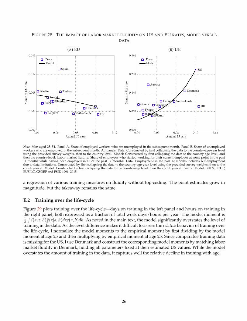
FIGURE 28. THE IMPACT OF LABOR MARKET FLUIDITY ON UE AND EU RATES, MODEL VERSUS

DATA

(A) EU (B) UE

Note: Men aged 25–54. Panel A. Share of employed workers who are unemployed in the subsequent month. Panel B. Share of unemployedworkers who are employed in the subsequent month. All panels. Data: Constructed by first collapsing the data to the country-age-year levelusing the provided survey-weights, then to the country-level. Model: Constructed by first collapsing the data to the country-age level, andthen the country-level. Labor market fluidity: Share of employees who started working for their current employer at some point in the past11 months while having been employed in all of the past 12 months. Data: Employment in the past 12 months includes self-employmentdue to data limitations. Constructed by first collapsing the data to the country-age-year level using the provided survey weights, then to thecountry-level. Model: Constructed by first collapsing the data to the country-age level, then the country-level. Source: Model, BHPS, ECHP,EUSILC, GSOEP and PSID 1991–2015.

a regression of various training measures on fluidity without top-coding. The point estimates grow inmagnitude, but the takeaway remains the same.

E.2 Training over the life-cycle

Figure 29 plots training over the life-cycle—days on training in the left panel and hours on training inthe right panel, both expressed as a fraction of total work days/hours per year. The model moment is1A

´i(a, z, h)g(z|a, h)dze(a, h)dh. As noted in the main text, the model significantly overstates the level of

training in the data. As the level difference makes it difficult to assess the relative behavior of training overthe life-cycle, I normalize the model moments to the empirical moment by first dividing by the modelmoment at age 25 and then multiplying by empirical moment at age 25. Since comparable training datais missing for the US, I use Denmark and construct the corresponding model moments by matching labormarket fluidity in Denmark, holding all parameters fixed at their estimated US values. While the modeloverstates the amount of training in the data, it captures well the relative decline in training with age.

26

TABLE 14. TRAINING AND LABOR MARKET FLUIDITY WITHOUT TOP-CODE

Panel A. Days (fraction of year) Panel B. Hours (fraction of year) Panel C. Whether trained

Raw Controls Direct Raw Controls Direct Raw Controls Direct

Fluidity 1.947*** 1.648*** 1.692*** 1.383*** 1.143*** 1.089*** 9.915*** 9.438*** 9.545***(0.253) (0.196) (0.119) (0.148) (0.128) (0.127) (1.196) (1.366) (1.280)

JJ -0.007 -0.004 -0.011(0.011) (0.005) (0.012)

Age -0.002*** -0.003** -0.001** -0.002** -0.005*** -0.004***(0.001) (0.001) (0.001) (0.001) (0.001) (0.001)

College 0.022*** 0.030*** 0.005** 0.007*** 0.108*** 0.106***(0.005) (0.006) (0.002) (0.002) (0.027) (0.029)

N 135,563 115,897 63,634 135,318 115,676 63,494 135,989 116,261 63,852

Note: Men aged 25–54. Projection of training outcome on labor market fluidity without or with controls. Panel A. Days on vocational trainingin the past 12 months, expressed as a fraction of potential work days (5*52). Panel B. Hours on vocational training in the past 12 months,expressed as a fraction of potential work hours (40*52). Panel C. Whether worker undertook any vocational training since January last year.All panels. Labor market fluidity: Share of employees who started working for their current employer at some point in the past 11 monthswhile having been employed in all of the past 12 months. Employment in the past 12 months includes self-employment. Constructed by firstcollapsing the data to the country-age-year level using the provided survey weights, then to the country level. Standard errors are clustered atthe country-level. * statistically significant at 10%; ** statistically significant at 5%; *** statistically significant at 1%. Source: ECHP 1995–2001.

FIGURE 29. TRAINING OVER THE LIFE-CYCLE, MODEL VS DATA

(A) DAYS ON TRAINING (B) HOURS ON TRAINING

Note: Men aged 25–54. Panel A. Days on vocational training in the past 12 months, expressed as a fraction of potential work hours (40*52). PanelB. Hours on vocational training in the past 12 months, expressed as a fraction of potential work hours (40*52). Both panels. Model momentis average investment, 1

A´

i(a, z, h)g(z|a, h)dze(a, h)dh, normalized to the empirical moment by first dividing by the model moment at age 25and then multiplying by empirical moment at age 25. Hours and days on training are top-coded at 13 weeks of full time training per year, andrefer to Denmark as the highest fluidity country with training data. Model moments are for a hypothetical country with the same aggregatelabor market fluidity as Denmark, holding all other parameters fixed at their estimated US values. All training measures: Constructed by firstcollapsing the data to the country-age-year level using the provided survey weights, then to the country level. Labor market fluidity: Shareof employees who started working for their current employer at some point in the past 11 months while having been employed in all of thepast 12 months. Employment in the past 12 months includes self-employment. Constructed by first collapsing the data to the country-age-yearlevel using the provided survey weights, then to the country level. Source: ECHP 1995–2001.

27

E.3 Additional training outcomes

Figure 30 plots hours on training in the past 12 months, whether the worker did any training sinceJanuary in the year prior to the survey and the share of workers who report that their employer paid forthe training against labor market fluidity. If anything, the share rises with labor market fluidity, but thepattern is not statistically significant.

FIGURE 30. TRAINING AND LABOR MARKET FLUIDITY, DATA

(A) HOURS ON TRAINING (B) WHETHER TRAINED

(C) SHARE PAID FOR BY EMPLOYER

Note: Men aged 25–54. Panel A. Hours on vocational training in thepast 12 months, expressed as a fraction of potential work hours (40*52).Hours and days on training are top-coded at 13 weeks of full time train-ing per year. Panel B. Whether worker undertook any vocational train-ing since January last year. Panel C. Share of workers who report thattheir employer paid for their vocational training since January last year.All training measures: Constructed by first collapsing the data to thecountry-age-year level using the provided survey weights, then to thecountry level. Labor market fluidity: Share of employees who startedworking for their current employer at some point in the past 11 monthswhile having been employed in all of the past 12 months. Employmentin the past 12 months includes self-employment. Constructed by firstcollapsing the data to the country-age-year level using the providedsurvey weights, then to the country level. Source: ECHP 1995–2001.

28

E.4 Training and subsequent mobility: the generality of human capital

This subsection uses the panel data on training and mobility to offer support for the notion that humancapital is general. In particular, I hypothesize that if firm-specific human capital is important, then theincidence of training should be associated with a subsequent decline in the probability that the workerleaves the firm. The reason is that firm-specific human capital raises the value of the current matchrelative to alternative matches.

Table 15 relates JJ in the past 12 months to training in the year prior to that, i.e. 13–24 months ago (Ihave alternatively related mobility to training in the current year as well as two years ago with similarresults). The first column shows the raw correlation with only country and year controls, the secondadds age, education, occupation and sector controls, and the third controls for worker-fixed effects andyear effects.38 There is no evidence that workers who trained more in the past year are less likely tomake a JJ move in the current year. In fact, the raw data suggest the opposite, although this appears tobe driven by selection. In any case, if skills had been primarily firm-specific, one may have hypothesizedthat worker mobility would decline with training.

TABLE 15. JJ MOBILITY AND LAGGED TRAINING

Panel A. Days (fraction of year) Panel B. Hours (fraction of year) Panel C. Whether trained

Raw Controls Within Raw Controls Within Raw Controls Within

Training 0.068* 0.044 0.014 0.115** 0.058 0.034 0.001 0.001 -0.004(0.036) (0.033) (0.040) (0.053) (0.047) (0.062) (0.004) (0.003) (0.004)

N 49,114 48,289 46,247 49,011 48,190 46,134 49,285 48,460 46,434

Note: Men aged 25–54. Projection of JJ in the past year on various measures of vocational training 13–24 months ago, without or with controls.Raw: Country and year controls; Controls: Country, year, age, education and occupation controls; Within: Individual fixed effects and yearcontrols. Panel A. Days on vocational training in the past 12 months, expressed as a fraction of potential work days (5*52). Panel B. Hours onvocational training in the past 12 months, expressed as a fraction of potential work hours (40*52). Panel C. Whether worker undertook anyvocational training since January last year. All panels. JJ mobility: Whether worker started working for their current employer at some pointin the past 11 months while having been employed in all of the past 12 months. Employment in the past 12 months includes self-employment.Standard errors are clustered at the country-level. * statistically significant at 10%; ** statistically significant at 5%; *** statistically significant at1%. Source: ECHP 1995–2001.

E.5 Firm wage and firm size/productivity

Table 16 reports results from the first stage regression (15) projecting pay on firm size bins (data) / matchproductivity bins (model) with controls. Larger firms pay better, consistent with previous research. Asexpected more productive matches on average pay better. In fact, the magnitude of the empirical andmodel relationship is about the same.

E.6 Training and firm size: the complementarity in production

The following intuition is clearest in the simple two period model, so I will restrict attention to that (butit carries through numerically to the general model). Recall from (??) that optimal investment is givenby

i =1z1

(µ

(z1 + pβ

z2 − z1

2

)) 11−η

(32)

38The same conclusion holds with age instead of year controls.

29

TABLE 16. INFERRING FIRM PAY

Data Model

α2 0.101*** 0.078***(0.005) (0.001)

α3 0.188*** 0.131***(0.006) (0.001)

α4 0.214*** 0.182***(0.006) (0.001)

α5 0.265*** 0.260***(0.006) (0.001)

α6 0.338*** 0.370***(0.006) (0.001)

N 77,793 5,154,592

Note: Men aged 25–54. Projection of pay on firm size (data) / match productivity (model), each binned into 6 roughly equally large bins (in anemployment-weighted sense), controlling for age, education, occupation and country-year (data) / age and country (model). Standard errorsare clustered at the individual-level. *** statistically significant at 1%. Source: ECHP 1995–2001.

Whether training rises or falls with match productivity, z1, is ambiguous because of the opposing effectsof the first and second terms.

Consider instead a model with no complementary in production, z + h. Given the normalizationh0 = 1, the natural extension of the Ben-Porath (1967) investment problem would be

maxi∈[0,1]

{(1− i)(z1 + 1) + z1 +

p2

β(z1 − z1) + 1 +µ

η

(i(z + 1)

)η}

with first-order condition

i =1

z1 + 1µ

11−η (33)

which is unambiguously declining in current productivity, z1. Hence, one may hypothesize that thismodel would be inconsistent with the positive correlation between firm level pay and training. Whilea more thorough assessment is left for future work, I note that the current model matches well theempirical relationship between training and firm pay.

E.7 Share of employment at large firms

As noted in Figure 4, a larger share of workers work at large, higher paying firms in more fluid labormarkets, where workers always train more.39 Given that the model abstracts from size, to comparethis prediction with the model, I first note that the average share of workers in 50+ firms across thesecountries is very close to 50 percent in the data. Hence in the model, I compute the share of workers inthe upper half of employment-weighted match productivity, constructed in the pooled data set of all thesimulated countries. Figure 31 plots the share of workers in upper half of firm size in the data / upperhalf of match productivity in the model. Given that firm size is likely an imperfect proxy for matchproductivity, the mechanism does a decent job matching the empirical patterns.

39The data on firm size is only available in the cross-sectional version of the EUSILC, which does not allow me to trackindividuals over time. It is also missing from the BHPS, so I use the available data from the EUSILC for the UK. The GSOEP

30

FIGURE 31. SHARE OF WORKERS IN 50+ FIRMS, MODEL VS DATA

Note: Male wage employees aged 25–54. Data: Share of workers at50+ employee firms. Model: Share of workers in the upper half ofemployment-weighted match productivity, constructed across all sim-ulated countries. The upper half of employment-weighted match pro-ductivity corresponds closely to the average share of workers at 50+firms across these countries (51.1%). Labor market fluidity: Share ofemployees who started working for their current employer at somepoint in the past 11 months while having been employed in all of thepast 12 months. Employment in the past 12 months includes self-employment. Constructed by first collapsing the data to the country-age-year level using the provided survey weights, then to the countrylevel. Source: ECHP, EUSILC and PSID 1994–2015.

codes firm size in non-comparable bins, and the PSID only asks for firm size in 1999 and from 2003 onwards.

31

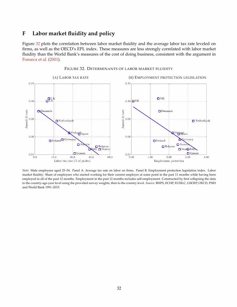
F Labor market fluidity and policy

Figure 32 plots the correlation between labor market fluidity and the average labor tax rate leveled onfirms, as well as the OECD’s EPL index. These measures are less strongly correlated with labor marketfluidity than the World Bank’s measures of the cost of doing business, consistent with the argument inFonseca et al. (2001).

FIGURE 32. DETERMINANTS OF LABOR MARKET FLUIDITY

(A) LABOR TAX RATE (B) EMPLOYMENT PROTECTION LEGISLATION

Note: Male employees aged 25–54. Panel A. Average tax rate on labor on firms. Panel B. Employment protection legislation index. Labormarket fluidity: Share of employees who started working for their current employer at some point in the past 11 months while having beenemployed in all of the past 12 months. Employment in the past 12 months includes self-employment. Constructed by first collapsing the datato the country-age-year level using the provided survey weights, then to the country level. Source: BHPS, ECHP, EUSILC, GSOEP, OECD, PSIDand World Bank 1991–2015.

32