NBER WORKING PAPER SERIES

LABOR MARKET FLUIDITY AND ECONOMIC PERFORMANCE

Steven J. DavisJohn Haltiwanger

Working Paper 20479http://www.nber.org/papers/w20479

NATIONAL BUREAU OF ECONOMIC RESEARCH1050 Massachusetts Avenue

Cambridge, MA 02138September 2014

We thank Richard Rogerson, other conference participants, Claudia Goldin, Jason Faberman and JimSpletzer for helpful comments and the Kauffman Foundation, the University of Chicago Booth Schoolof Business, and the University of Maryland for financial support. Jake Blackwood, Diyue Guo, andClaudia Macaluso provided excellent research assistance. This paper was prepared for the FederalReserve Bank of Kansas City’s economic policy symposium on “Re-Evaluating Labor Market Dynamics,”held August 21-23 2014 in Jackson Hole, Wyoming. The views expressed herein are those of the authorsand do not necessarily reflect the views of the National Bureau of Economic Research.

NBER working papers are circulated for discussion and comment purposes. They have not been peer-reviewed or been subject to the review by the NBER Board of Directors that accompanies officialNBER publications.

© 2014 by Steven J. Davis and John Haltiwanger. All rights reserved. Short sections of text, not toexceed two paragraphs, may be quoted without explicit permission provided that full credit, including© notice, is given to the source.

Labor Market Fluidity and Economic PerformanceSteven J. Davis and John HaltiwangerNBER Working Paper No. 20479September 2014, Revised December 2014JEL No. E24,J63,L23

ABSTRACT

U.S. labor markets became much less fluid in recent decades. Job reallocation rates fell more thana quarter after 1990, and worker reallocation rates fell more than a quarter after 2000. The declinescut across states, industries and demographic groups defined by age, gender and education. Youngerand less educated workers had especially large declines, as did the retail sector. A shift to older businesses,an aging workforce, and policy developments that suppress reallocation all contributed to fluidity declines.Drawing on previous work, we argue that reduced fluidity has harmful consequences for productivity,real wages and employment. To quantify the effects of reallocation intensity on employment, we estimateregression models that exploit low frequency variation over time within states, using state-level changesin population composition and other variables as instruments. We find large positive effects of workerreallocation rates on employment, especially for young workers and the less educated. Similar estimatesobtain when dropping data from the Great Recession and its aftermath. These results suggest the U.S.economy faced serious impediments to high employment rates well before the Great Recession, andthat sustained high employment is unlikely to return without restoring labor market fluidity.

Steven J. DavisBooth School of BusinessThe University of Chicago5807 South Woodlawn AvenueChicago, IL 60637and NBERSteven.Davis@ChicagoBooth.edu

John HaltiwangerDepartment of EconomicsUniversity of MarylandCollege Park, MD 20742and NBERhaltiwan@econ.umd.edu

1

Introduction

As measured by flows of jobs and workers across employers, U.S. labor markets became

much less fluid in recent decades. We document a large, broad-based decline in these labor market

flows, drawing on multiple data sources and updating results in previous work. An aging workforce

and a secular shift away from younger and smaller employers partly account for the long-term

decline in labor market fluidity. These forces are not the main story, however. Instead, we find

large declines in the rate at which workers reallocate across employers within cells defined by

gender and age and by gender and education. Likewise, there are large declines in the rate at which

jobs reallocate across employers within cells defined by industry, employer size and employer age.

International comparisons suggest that the U.S. experience of a large secular decline in the pace of

job reallocation is somewhat unusual.

In light of these facts, we consider whether reduced labor market fluidity is cause for serious

concern about the past and future performance of the U.S. economy. There are, as we discuss, some

beneficial and benign aspects of reduced labor market fluidity. But we also identify strong reasons

for concern about the consequences of reduced fluidity for productivity growth and real wages.

Perhaps the most serious concerns involve the implications of reduced fluidity for employment

rates, especially among marginal workers and those with limited skills. We develop this theme in

Sections II and III, drawing on several strands of previous research. Our discussion leads to the

hypothesis that fluid labor markets promote high levels of employment. Conversely, according to

this hypothesis, a secular decline in labor market fluidity is a force for lower employment rates.

The closest antecedent to our treatment of this hypothesis is a study by Robert Shimer

(2001). He also formulates and investigates a “fluid labor market hypothesis,” drawing inspiration

from a model that links recruiting costs to the share of young workers in the labor market.

Employers in Shimer’s model find it easier to recruit new employees when the youth labor share is

high. Easier recruiting, in turn, leads to higher equilibrium job creation and lower unemployment

2

rates for workers of all ages. Our discussion stresses that fluid labor markets can promote full

employment through other mechanisms as well, especially human capital accumulation, and that the

youth share is only one factor among many behind secular changes in labor market fluidity. In

addition, we bring more and better data to our investigation of the fluid labor market hypothesis.

Our empirical examination of the hypothesis exploits data on state-level rates of

employment, job reallocation and worker reallocation. We estimate the effects of the reallocation

measures on state-level employment rates for groups defined by gender, education and age, while

controlling for state fixed effects, national and state-level cyclical conditions, and the presence of

children and young children in the household. To address concerns about the endogeneity of the

reallocation measures, we deploy instruments that capture the youth share of the population in the

state and time period, the relative abundance of less-educated young persons, and changes to state-

level reallocation intensity that derive from national shifts in the industry mix of employment and

industry-level reallocation intensities. Our key identifying assumption is that these instrumental

variables do not affect group-level employment rates within the state, conditional on the controls,

except through their effects on the pace of job and worker reallocation.

We find large, statistically significant effects of worker reallocation rates on the employment

rates of the young and the less educated. The effects are uniformly larger for men. For example, a

100 basis point decline in the worker reallocation rate yields an estimated 77 basis point decline in

the employment rate for men who did not finish high school. For men under 25 who did not finish

high school, the corresponding estimate is 143 basis points. The larger estimated effects for the

young, the less educated, and men comport well with the actual pattern of larger employment rate

declines for these groups. When we use the job reallocation rate as our fluidity measure, doubling

our sample period, we find positive and statistically significant effects of fluidity in all education

groups for men and women. For both fluidity measures, the cross-state patterns of declines in

actual employment rates are captured reasonably well by the predictions of our regression models.

3

The next section explores the dimensions of secular decline in the pace of U.S. worker and

job reallocation. Section II asks whether reduced labor market fluidity is cause for serious concern.

Section III develops the hypothesis that fluid labor markets promote high employment rates,

drawing on Shimer (2001) and many other works. Section IV reports our empirical investigation of

the hypothesis. We set forth our main conclusions, implications for policy makers, and identify

important open questions in Section V.

I. Secular Decline in the Pace of U.S. Labor Market Flows

Figure 1 reports quarterly labor market flows, expressed as a percent of employment, based

on data from the Job Openings and Labor Turnover Survey (JOLTS) and the Business Employment

Dynamics (BED) program. Job creation is the sum of employment gains at new and expanding

establishments, and job destruction is the sum of employment losses at exiting and shrinking

establishments. Hires, quits and layoffs follow the concepts in the JOLTS.1 The series plotted in

Figure 1 exhibit prominent cyclical patterns, but they also show large declines from 1990 to 2013.2

Figure 2 re-organizes the information to make it easier to discern trend changes in the pace

of labor market flows. The quarterly job reallocation rate (sum of creation and destruction rates)

fell steadily to stand at 12.2% of employment in 2013Q2, one-third below its peak value in 1991Q1

and more than one quarter below its average value in 1990. The quarterly worker reallocation rate

(sum of hires and separations) shows a different pattern, changing little over the full course of the

1990s. It then fell sharply from 33.5% of employment per quarter in 1999 to 24.1% in 2010, before

1 The JOLTS sample has too little mass in the tails of the (employment-weighted) cross-sectional distribution of employer growth rates and too little mass near zero, as shown in Davis et al. (2009). The effect is to understate worker flows, which are much larger at employers in the tails of the growth rate distribution. To address this issue, we reweight the JOLTS micro data to match the cross-sectional distribution of employer growth rates in the BED. Our reweighting adjustments follow the methods of Davis et al. (2009) and Davis, Faberman and Haltiwanger (2012). 2 Many indicators, based on a variety of data sources and measurement methods, show a secular decline in the risk of job loss facing American workers since the early 1980s. See Davis (2008), Davis et al. (2010), Davis, Faberman and Haltiwanger (2012), Fujita (2012), and Elsby, Hobijn and Şahin (2013).

4

rebounding slightly.3 Figure 2 also reports excess worker flows over and above the amount

required to accommodate job flows – “churning” in the language of Burgess, Lane and Stevens

(2000) and Lazear and Spletzer (2012). Churning flows rose over much of the 1990s and then fell

steeply during the 2000s.

It’s worth stressing that Figure 2 provides evidence of secular declines in the pace of job

reallocation and in the pace of churn. According to Figure 2, the quarterly worker reallocation rate

fell by 8.7 percentage points from 1990Q2 to 2013Q2. A drop in churning accounts for 4.6 points

of this long-term decline in worker reallocation, and a drop in job reallocation accounts for 4.1

points. In other words, a slower pace of job flows accounts for somewhat less than half the long-

term decline in worker reallocation. All three measures – job reallocation, churn, and their sum,

worker reallocation – fell substantially in the past quarter century. This commonality of trends is

more than coincidental, as we discuss shortly.

Figure 3 reports annual rates of job reallocation across firms and establishments, drawing on

comprehensive Census data sources for nonfarm private sector employers. These Census sources

lack data on worker flows, but they let us examine job reallocation in earlier years. As seen in

Figure 3, the secular decline in job reallocation rates dates back to at least the early 1980s. Using

data from the Current Population Survey, Davis et al. (2010) show that unemployment inflows and

outflows fell by nearly half, as a percent of employment, from the early 1980s to the early 2000s,

and that much of this decline is due to the drop in job reallocation. Molloy, Smith and Wozniak

(2014) trace large, broad-based declines in interstate migration rates since the 1980s mainly to

declines in job-related reasons for geographic mobility.

Previous studies by Davis et al. (2007, 2010) and Decker et al. (2014b) show that declines in

job reallocation rates and in the volatility of business growth rates are widespread across industries

3 Similarly, Hyatt and Spletzer (2013) find large declines in quarterly U.S. labor market flows from 1998 to 2010, drawing on data from the BED, JOLTS and other sources.

5

since the early 1980s.4 Figure 4 illustrates this pattern for selected industry sectors, drawing on data

from the Business Dynamics Statistics program. As seen in the figure, Retail Trade experienced an

especially pronounced fall in the pace of job reallocation.

How have shifts in the industry, size and age distributions of employment contributed to the

secular decline in the pace of job reallocation? Changes in the industry distribution cut in the

“wrong” direction (Decker et al., 2014b). That is, the U.S. employment mix shifted from industries

with relatively low job reallocation rates (e.g., Manufacturing) to industries with relatively high

reallocation rates (e.g., Retail Trade). As discussed in Davis et al. (2007), much of the decline in job

reallocation and business volatility within Retail Trade reflects a marked shift of activity to larger

firms and establishments, which are less volatile than smaller businesses. An important and broader

phenomenon is the secular shift away from younger firms, illustrated in Appendix Figure A.1.

Davis et al. (2007) and Decker et al. (2014b) find that this shift accounts for about one quarter of the

secular decline in business volatility and the pace of job reallocation since the early 1980s. Taken

together, shifts in the industry, size and age distributions of employment account for about 15

percent of the secular decline in job reallocation (Decker et al., 2014b).

Figure 5 reveals a remarkably close relationship between job flows and worker flows in the

cross-section of employer growth rates. When plotted as functions of establishment growth rates,

rates of hires and separation exhibit “hockey-stick” shapes. The hires relation is nearly flat to the

left of zero (contracting employers) and rises more than one-for-one with employment growth to the

right of zero (expanding employers), with a pronounced kink at zero. The separations relation is a

mirror image of the hires relation. These cross-sectional relations are highly stable over time,

differing little between boom and bust periods (Davis, Faberman and Haltiwanger, 2012). In short,

4 Haltiwanger, Hathaway and Miranda (2014) find that job reallocation rates rose in certain high-tech industries during the 1990s, counter to the trend in other industries. Even in those same high-tech industries, however, the pace of job reallocation fell substantially during the 2000s.

6

hires are tightly linked to job creation in the cross section, and separations are tightly linked to job

destruction.5

This figure helps us understand the time-series relationship between job reallocation and

worker reallocation in Figure 2. The cross-sectional distribution of employer growth rates became

less dispersed and more concentrated about zero in recent decades (Davis et al., 2007, Decker et al.,

2014b). When employer growth rates become more concentrated about zero, fewer job positions

shift from shrinking to growing employers, and job reallocation declines. The pace of worker flows

diminishes as well, according to Figure 5, because rates of hires and separations are much smaller

for employers with small positive or negative growth rates. Moreover, because hires and

separations rise more than one-for-one with job flows as employer growth rates move away from

zero (in the positive direction for hires and the negative direction for separations), churn rates also

diminish as employer growth rates become more concentrated about zero. Thus, in light of Figure 5,

trends in job reallocation rates feed into the trends in both churn rates and overall worker

reallocation rates. These observations explain why we see much commonality of trends in the rates

of job reallocation, churn, and overall worker reallocation.

Figure 6 displays quarterly job and worker reallocation rates by gender and age group from

1999 to 2012. We tabulate the statistics plotted in this figure from the Quarterly Workforce

Indicators (QWI), which draw on comprehensive administrative records for most states in the

United States. As before, job reallocation is the sum of job creation and destruction, and worker

reallocation is the sum of hires and separations.6 These plots show large declines in the pace of job

5 See Fujita and Nakajima (2014) for a theoretical model that delivers the hockey-stick shapes in Figure 5 and reproduces major patterns in the cyclical behavior of job flows and worker flows. 6 JOLTS and QWI data deliver similar messages about trends, but measured worker reallocation is markedly higher in the QWI. We adjust for missing tail mass in the JOLTS sample (footnote 1), which brings the JOLTS measure of worker reallocation closer to the QWI measure. After this adjustment, the average quarterly worker reallocation rate from 1998:2 to 2012:2 is 28.9 percent in the JOLTS and 45.1 percent in the QWI. The discrepancy appears to partly reflect the fuller capture of short duration jobs in the QWI. When restricting attention to jobs that last at least one quarter,

7

flows and worker flows across age groups for both men and women. The declines largely predate

the Great Recession. In fact, the churn component of worker reallocation rates actually rebounds

modestly after the Great Recession, as shown in Appendix Figure A.2. Figure 7 and Appendix

Figure A.3 show that rates of job reallocation, worker reallocation and churn also fell sharply across

education groups for both men and women. Similar patterns hold when using QWI flows calculated

from employment relationships that survive for at least one full calendar quarter.

Secular declines in labor market fluidity are also pervasive across states. Figure 8 shows

that rates of job reallocation, churn and worker reallocation fell from 1999-2001 to 2010-12 in all

30 states covered by the QWI. Figure 9 shows that job reallocation rates fell from 1988-90 to 1998-

2000 and from 1998-2000 to 2008-2010 in all 50 states. Notably, the magnitude of the declines

varies greatly across states. In Section IV, we use this cross-state heterogeneity in the changes as

leverage for estimating the effects of fluidity on employment and unemployment rates. Appendix

figures A.5 to A.7 consider the role of compositional shifts in the state-level changes. Shifts in the

age distribution of workers account for modest shares of the declines in state-level worker

reallocation from 1998-200 to 2009-11, while the education mix plays no role.7 Industry distribution

shifts go in the “wrong” direction to account for changes in state-level job reallocation rates.

Figure 10 provides some international perspective on the U.S. experience in recent decades.

We focus on changes over time within countries, because measured flows are strongly influenced

by labor market institutions, the structure of production and employment, data quality, and

measurement methods – all of which can differ greatly across countries. According to Figure 10,

the United States is somewhat unusual in terms of its secular decline in job reallocation. While a

the average QWI worker reallocation rate is only 21.4 percent. Another source of understatement in the JOLTS (for which we do not adjust) involves very young establishments, which have very high worker reallocation even when conditioning on establishment growth. Very young establishments are missing from the JOLTS sample frame, because it takes at least a year to identify new establishments, perform pre-sample processing, and bring them into the sample. 7 Hyatt and Spletzer (2013) find similar results at the national level.

8

more extensive set of international comparisons might tell a different story, the evidence here

suggests that secular declines in U.S. labor market flows largely reflect forces and developments

that are specific to, or more pronounced in, the United States.

Summing up, the United States underwent a large, broad-based decline in the pace of labor

market flows in recent decades. The decline holds across major industry sectors, across all states,

and across age and education groups for both men and women. A shift away from younger firms

plays an important role in the slowdown of job reallocation, while secular shifts in the industry

distribution cut the other way. An aging workforce is a factor behind the slowdown of worker

reallocation. Thus, composition shifts among employers and workers contribute to the secular

declines in the pace of job and worker reallocation. The main story, however, is a general shift

toward less fluidity in U.S. labor markets.

It might be tempting to conclude from this evidence that U.S. labor markets have become

less flexible in some broader sense. However, that more sweeping conclusion does not follow from

the foregoing evidence. As noted in Davis et al. (2007), a relaxation of restraints on employer-level

wage and hours adjustments can yield smaller job flows in response to idiosyncratic employer-

specific labor demand shocks. A similar point applies to worker flows. See Bertola and Rogerson

(1997) and Pries and Rogerson (2005) for thoughtful analyses of the relationship between various

aspects of labor market flexibility and the magnitude of labor market flows.

II. Is the Reduced Fluidity of U.S. Labor Markets Cause for Concern?

Labor market fluidity can affect economic performance in many ways. Our discussion here

stresses implications for employment, productivity and wages, highlighting both positive and

negative effects of reduced fluidity.

A. Beneficial and Benign Aspects of Reduced Fluidity

According to the canonical search equilibrium model of Mortensen and Pissarides (1994),

less job destruction means fewer job-losing workers, smaller unemployment inflows, and lower

9

unemployment rates. Lower steady-state job reallocation in the MP model also implies less job

loss, smaller unemployment flows, and lower unemployment.8 Davis et al. (2010) investigate the

role of this simple mechanism in the long-term decline of U.S. unemployment inflow rates. They

find that inflow rates for experienced workers trended down by larger amounts in industries with

larger long-term drops in job destruction rates. The same pattern holds when using job reallocation

or business volatility in place of job destruction in their industry-level regressions.

To quantify the long-term effect of falling job destruction on unemployment inflows, Davis

et al. (2010) first estimate regressions on industry-level panel data with non-overlapping three-year

time periods. They control for industry and period fixed effects to isolate variation over time within

industries. In their preferred specification, a 100 basis point fall in the quarterly job destruction rate

lowers the monthly unemployment inflow rate among experienced workers by an estimated 28 basis

points. Second, they apply this estimate to the 174 basis point fall in quarterly job destruction from

1990 to 2005 to obtain an implied drop in monthly unemployment inflows of 48 basis points –

which amounts to 55 percent of the actual drop in the inflow rate from 1990 to 2005 and 22 percent

of its average value over the period. A similar exercise finds that falling job destruction accounts

for 28 percent of the much larger drop in unemployment inflow rates from 1982-83 to 2005.

Other research on the secular behavior of unemployment flows starts from the well-known

fact that younger workers experience more frequent unemployment spells. Building on this fact,

Shimer (1998) and Fujita (2012) provide evidence that an aging workforce is another major factor

behind the big drop in unemployment and unemployment inflow rates after the early 1980s. While

unemployment inflow rates rose sharply during the Great Recession, they returned to pre-recession

lows by 2014. Several other job-loss measures – the JOLTS layoff rate, the rate of new claims for

8 Fujita (2012) derives this implication in a richer MP-type model that incorporates the skill obsolescence feature of Ljungvist and Sargent (1998) and Den Haan, Haefke and Ramey (2005).

10

unemployment insurance benefits, and the BED job destruction rate – also reached historic lows by

early 2014. See Appendix Figure A.4.

In summary, demographic trends and a declining pace of job reallocation largely account for

the very sizable long-term drop in unemployment inflow rates. In contrast, the outflow rate from

the unemployment pool shows no strong trend prior to the Great Recession. Thus, the large drop in

the U.S. unemployment rate from the early 1980s to the mid 2000s mainly reflects the drop in

unemployment inflow rates, which we attribute to falling job reallocation and an aging workforce.

In this light, the secular decline in job reallocation appears as a beneficial development that brings

greater job security and a lower incidence of unemployment. And the secular decline in the churn

component of worker reallocation is, in part, a benign consequence of an aging workforce.

Job loss can lead to lower earnings for many years following a displacement event. See, for

example, the studies of displaced workers by Jacobson, LaLonde and Sullivan (1993), Couch and

Placzek (2010), and Davis and von Wachter (2011). Sullivan and von Wachter (2009) provide

evidence that displaced workers experience higher mortality rates than otherwise comparable

workers who do not lose jobs. Davis and von Wachter review other research that links worker

displacement to negative effects on health outcomes, marital stability, emotional well-being, and the

schooling achievement and cognitive development of displaced workers’ children. In view of this

evidence, it is reasonable to hypothesize that lower job reallocation rates reduce the incidence of

these negative effects. We say “hypothesize,” not “conclude,” because a slower pace of job

reallocation can worsen the consequences for those who lose jobs, as we discuss below.

Reduced labor market fluidity is, in part, a by-product of developments in specific sectors

that raised productivity and improved consumer welfare. The U.S. retail trade sector provides a

clear case in point. Wal-Mart and other big-box firms transformed supply chains, wholesale

distribution, inventory management, pricing, and product selection in recent decades. Wal-Mart

opened its first store in 1962 and by 2007 operated 4,000 stores (including Sam’s Club outlets) and

11

employed 1.3 million workers in the United States alone (Basker, 2007). Other national chains such

as Target and “category killers” like Home Depot, Staples, Barnes & Noble, and Best Buy also

played significant roles in transforming the retail sector. According to McKinsey Global Institute

(2001), labor productivity growth in the general merchandising segment of retail trade jumped from

5.3% per year in 1987-95 to 10.1% in 1995-1999. The McKinsey study attributes one-third of this

jump to the direct effect of Wal-Mart and two-thirds to the spread of Wal-Mart best practices to

competitors. Foster, Haltiwanger and Krizan (2006) attribute large retail sector productivity gains

in the 1990s mainly to the reallocation of jobs and workers away from less productive stores to

newer, more productive ones operated by national chains. Basker (2005), Basker and Noel (2009)

and Hausman and Liebtag (2007) show that these developments yielded lower prices for consumers.

As a result of these changes, the U.S. retail sector became organized around much larger

firms and establishments (Jarmin, Klimek and Miranda, 2009). Many studies document a strong

negative relationship between employer size and the pace of job reallocation (Davis and

Haltiwanger, 1999). JOLTS data show a negative relationship between employer size and worker

reallocation. Thus, the transformation of the U.S. retail sector in recent decades, which had positive

effects on productivity and consumer welfare, contributed to the slowdown in job and worker

reallocation by shifting activity to larger firms and establishments.

B. Reasons for Concern

Notwithstanding the beneficial and benign aspects, there are good reasons for concern about

the implications of reduced labor market fluidity. First, slower job and worker reallocation goes

hand in hand with a slower arrival rate of new job opportunities. For the unemployed, this

development increases the risk of long jobless spells. For the employed, it hampers their ability to

switch employers so as to move up a job ladder, change careers, or satisfy locational constraints. In

line with this observation, previous studies find that job mobility facilitates wage growth and career

advancement. Topel and Ward (1992), for example, find that wage gains upon switching employers

12

account for one-third of early-career wage growth among American men. Hagedorn and Manovskii

(2013) find faster wage growth during employment spells, and during job spells with a given

employer, when the spells overlap with tighter labor markets. They attribute these patterns to the

more rapid arrival of job offers in tighter labor markets and, as a consequence, greater opportunities

for workers to encounter a high quality match. Akerlof, Rose and Yellen (1988) stress that fluid

labor markets yield better job-worker matching with respect to non-pecuniary characteristics.

Second, the available evidence cuts against the view that reallocation slowed because firms

now face a more quiescent economic environment. Bloom et al. (2012) find rising volatility of

plant-level TFP shocks in the U.S. manufacturing sector after 1990. Decker et al. (2014b) find that

the intra-industry dispersion of plant-level total factor productivity rose, not fell, in the past quarter

century. They also find a declining trend in the responsiveness of plant-level growth rates to plant-

level TFP shocks in models fit to data from 1980 to 2010. Although limited to the manufacturing

sector, the evidence in these studies indicates that job and worker reallocation rates trended down

because U.S. employers became less responsive to shocks, not because employer-level shocks

became less variable.9

Cairo (2013) develops evidence that on-the-job training requirements increased over time,

both because the mix of jobs shifted to occupations with greater training requirements and because

training requirements rose within occupations. She also analyzes the connection between training

costs and job flows in an equilibrium search model with multi-worker firms. When calibrated to her

evidence on training costs, the model accounts for 30 percent of the secular decline in U.S. job

reallocation rates. Thus, Cairo’s evidence and analysis point to higher training costs as an important

factor behind reduced fluidity. The economic consequences are likely to turn on why training costs

rose. If they rose in response to technological changes, then returns in the form of more productive 9 Likewise, the 30-day VIX index for the S&P 500 shows no evidence of a secular decline in the past quarter century. However, it is difficult to draw conclusions about broader trends in business volatility from data on publicly traded firms for reasons discussed in Davis et al. (2007).

13

workers, better values for consumers, and higher profits presumably compensate for the extra

training costs. In contrast, if they rose in response to policies that restrict occupational labor supply

and insulate incumbents from competition, they are unlikely to generate net economic benefits.

That brings us to our third reason for concern: the role of government regulations and

policies that hamper reallocation. For example, government restrictions on who can work in which

jobs have expanded greatly over time. According to Figure 1 in Kleiner and Krueger (2013), the

fraction of workers required to hold a government-issued license to do their jobs rose from less than

5 percent in the 1950s to 29 percent in 2008. Adding workers who require government

certification, or who are in the process of becoming licensed or certified, brings the share of

workers in jobs that require a government-issued license or certification to 38 percent as of 2008.10

These observations suggest that training costs rose over time, in part, because regulations governing

occupational labor supply became increasingly restrictive. In any event, the spread of occupational

licensing and certification raises the cost of occupational mobility, one form of job mobility. Thus,

it seems likely that this development contributes to the secular declines in job and worker

reallocation documented in Section I.

Many other government policies reduce labor market fluidity, sometimes by design. A large

literature finds that employment protection laws suppress labor market flows, sometimes to a

powerful extent. See, for example, Blanchard and Portugal (2001), Gómez-Salvador et al. (2004),

Boeri and Jimeno (2005), OECD (2010) and Haltiwanger et al. (2014). Direct evidence about the

productivity effects of employment protection laws is less abundant, but several studies find sizable

negative effects on the rate of productivity growth. See Martin and Scarpetta (2012) for a review.

These findings fit well with much other evidence that factor reallocation flows are an important

source of medium-term productivity growth (e.g., Foster, Haltiwanger and Krizan, 2001). They

10 Carpenter et al. (2012) provides a detailed and informative study of state licensure requirements in 102 low- and moderate-income occupations.

14

also resonate with Schumpeterian theories of creative destruction that see reallocation as critical for

innovation and growth. Stifling reallocation stifles growth as well, according to these theories. See

Davis and Haltiwanger (1999) for a discussion and references to early work in this area and

Acemoglu et al. (2013) for a recent contribution.

From the perspective of creative destruction theories, the declining activity share of younger

firms is also worrisome. Firms no more than five years old account for 19.2 percent of employment

in 1982, 14.4 percent in 2000, and 10.7 percent in 2011 (Figure A.1). The nature of the shift away

from younger firms differs before and after 2000. In the 1980s and 1990s, it is dominated by Retail

and Services, which together account for almost half of private sector employment. The share of

employment at firms five years and younger fell by 11.8 percentage points in Retail from 1982 to

2000, and by 9.6 percentage points in Services. Our discussion in Section II.A suggests that the

shift away from younger firms in Retail was part of a productivity-enhancing transformation of the

sector. Since 2000, the high-tech sector experienced a large decline in startups and fast-growing

young firms, reversing an earlier pattern (Decker et al., 2014b). The frequency of initial public

offerings (IPOs) in the United States also plunged after 2000, following a robust pace of IPOs in the

1980s and 1990s.11 These observations suggest that the United States experienced a post-2000 shift

away from the type of young, entrepreneurial firms that were a major source of innovation and

productivity growth for the economy as a whole in the 1980s and 1990s.

Several studies investigate the employment, wage and productivity effects of statutes and

common-law doctrines designed to protect American workers from wrongful discharges. Two

studies by Autor et al. (2006, 2007) exploit cross-state differences in the timing of common-law

exceptions to the employment-at-will doctrine. These exceptions emerged in precedent-setting

decisions by state courts from 1972 to 1999, and proliferated rapidly in the 1980s, seriously eroding

11 According to Ritter (2013), the annual IPO rate for U.S. operating companies fell by more than two-thirds from the 1980-2000 period to the 2001-2012 period.

15

the presumption that employees could be fired at will. Autor et al. (2006) find that introducing the

implied-contract exception to employment-at-will has robust negative effects on state-level

employment rates that range from 0.8 to 1.6 percentage points across demographic groups. They

find less robust evidence of negative employment responses following the introduction of the good-

faith exception to employment-at-will.12 In contrast, they find no statistically significant evidence

of wage effects. Autor et al. (2007) find that the good-faith exception reduces the volatility of

annual employment growth rates in state-industry cells. For the manufacturing sector, which

affords richer data, they also find evidence that the good-faith exception encourages capital

deepening and depresses total factor productivity.13

We extend these two studies by estimating the effects of employment-at-will exceptions on

job reallocation rates. Table 1 reports regressions fit to data at the state-year level from 1978 to

1999 with controls for state and year fixed effects. Each column reports results for a particular firm

size class or, in the rightmost column, the overall reallocation rate. The key explanatory variables,

taken from Autor et al. (2006), capture the timing of state-level exceptions to the employment-at-

will doctrine. They are dummy variables that “turn on” the year after the judicial decision

establishing the indicated exception in the state, and they remain on for the remainder of the sample.

The sample period and regression specification parallel the baseline specification in Autor et al.

(2007) exactly, except for the dependent variable and the disaggregation by size class.

According to Table 1, the “Good-Faith Exception” to the employment-at-will doctrine

reduces annual job reallocation in the affected state by an estimated 104 basis points. The estimated

12 The implied-contract exception “comes into force when an employer implicitly promises not to terminate a worker without good cause,” according to Autor et al. (2006). The good-faith exception is usually limited in its application to “timing cases in which the employer intentionally deprives the worker of a promised benefit” such as a soon-to-vest pension benefit. 13 As discussed in Autor et al. (2006), other studies find that the implied-contract exception leads to greater reliance on temporary-help-agency workers and a reduced likelihood of hiring unemployed workers. They also point out that employment practices liability insurance became more prevalent in the 1990s, and that exceptions to employment-at-will appear to raise liability insurance costs.

16

effects are larger for smaller employers, twice as large for employers with fewer than 20 workers.14

The estimated effects of the “Implied-Contract Exception” and the “Public Policy Exception” are

small and statistically insignificant. Results for the “Good-Faith Exception” are essentially

unchanged if we drop the other two exceptions. Following Autor et al., we also estimated a

specification that considers dummy variables for 0, 1-2, and 3+ years after the introduction of the

“Good-Faith Exception.” According to results for this specification (not shown), the “Good-Faith

Exception” lowers overall job reallocation in the affected state by 177 basis points (standard error of

72 basis points) after three years. All four firm size classes show similarly large point estimates for

the effects three years after introduction of the “Good-Faith Exception.”

In addition to the erosion of the employment-at-will doctrine in the common law, many

federal and state laws enacted in recent decades establish protected classes of workers defined by

race, religion, gender, age, disability, national origin and other worker characteristics. These laws,

however well intentioned, likely contribute to the trend declines in job and worker reallocation rates

in recent decades, with negative effects on labor market fluidity and perhaps on employment,

wages, and productivity as well.

Other policy interventions suppress labor market flows as a by-product or unintended

consequence. We briefly discuss two cases in point: minimum wage laws, and employer-provided

health insurance. Dube et al. (2013) study minimum wage effects on earnings, employment and

worker flows for teens and restaurant workers. Applying a border-discontinuity empirical design to

QWI data, they estimate that a 10 percent increase in the minimum wage reduces the quarterly

worker reallocation rate by 2.0 percentage points for teens and by 2.1 points for restaurant workers.

Similarly, Brochu and Green (2013) estimate large negative effects of minimum wage hikes on

worker reallocation in Canadian data. These studies indicate that minimum wage hikes suppress 14 Because large employers often operate in multiple states, their personnel practices are less tied to the legal regime in any single state. For this reason, the empirical design in Table 1 is less suited for estimating how the erosion of employment-at-will affects job reallocation at large employers.

17

reallocation rates of younger and low-wage workers and for businesses that rely heavily on those

workers. Because the real federal minimum wage is lower now than in the 1970s, however, it

seems unlikely that changes in the prevalence and bite of minimum wage provisions have

contributed to the secular declines in worker reallocation documented in Section I.

The preferential tax treatment of employer-provided health insurance has profoundly

influenced the evolution of the U.S. healthcare system. Among the effects, most Americans obtain

health insurance through their employers. Because insurance plans differ among employers, and

because many employers do not offer health insurance, there are longstanding concerns that the

U.S. system leads to “job lock” for many workers, suppressing job-to-job mobility. See Currie and

Madrian (1999) and Gruber (2000) for reviews of the many studies on this topic. Gruber writes “the

weight of the evidence on job lock suggests that it is a significant phenomenon, with employer-

provided insurance reducing mobility by roughly 25-30%. But there remains considerable

disagreement.” For our purposes, the issue is how much the job-lock phenomenon contributes to

trend declines in worker reallocation. Given the large and growing share of national expenditures

devoted to health care in recent decades, it is plausible that employer-provided health insurance

materially contributed to the decline in worker reallocation. However, we are unaware of any

efforts to quantify trends in the extent of “job lock” due to employer-provided health insurance.

We think the information revolution has also played a significant role in the trend declines in

worker reallocation. Information about criminal records, credit histories, unfavorable media

coverage, and even ill-advised web postings has become more abundant and cheaper to access and

process.15 The likely result is a shift to stricter selection on the hiring margin and less use of trial

employment arrangements that contribute to churn. The erosion of employment-at-will and the

expansion of protected classes, both of which raise termination costs and intensify concerns about 15 Finlay (2009) and Fields and Emshwiller (2014) discuss the growth in the availability of criminal records to prospective employers. On the growing use of credit records as a screening tool in the hiring process, see Martin (2010).

18

litigation risk, provide strong incentives for employers to avail themselves of the screening

opportunities afforded by the information revolution.

Shifts in prevailing business models have also reduced labor market fluidity in some sectors.

The retail sector transformation brought large benefits, while lowering job and worker reallocation

rates. For some workers – especially among the young, the less educated, secondary earners, and

the unemployed – the loss of fluidity likely meant poorer labor market opportunities. Looking

beyond the retail sector, perhaps other changes in prevailing business models reduced fluidity.

Globalization, for example, has transformed supply chains and the organization of production

activity in many sectors. If large and mature firms are more able to respond to globalization,

employment is likely to shift away from smaller and younger employers, lowering job and worker

reallocation rates. We are unaware of studies on this matter, but it warrants attention.

To sum up, many factors contribute to reduced labor market fluidity in the United States.

We think restrictions on occupational labor supply, wrongful discharge and anti-discrimination

laws, and the preferential tax treatment of employer-provided health insurance are among the policy

factors that played a significant role in reducing labor market fluidity.16 Regardless of other benefits

(and costs) associated with these policy factors, their role in suppressing labor market fluidity can

lead to negative effects on productivity and welfare. See Hopenhayn and Rogerson (1993) for an

influential analysis of how policy distortions that impede job reallocation can undermine allocative

efficiency in a competitive equilibrium setting, with negative consequences for productivity, real

wages and welfare. In models with contractual and search frictions, (properly designed) policies

that increase reallocation costs can improve welfare. See, for example, Alvarez and Veracierto

(2001), who show that mandatory severance payments can raise employment and welfare by

16 Product market regulations that raise business entry costs or otherwise entrench incumbents also suppress reallocation in the labor market. See Bertrand and Kramarz (2002) and Klepper, Laeven, and Rajan (2006) for evidence.

19

reducing frictional unemployment. We conclude that empirical evidence is essential for reaching a

judgment about the economic consequences of reduced labor market fluidity.

III. The Fluid Labor Markets Hypothesis

Shimer (2001) finds that a higher share of youths, 16 to 24 years old, in the working-age

population raises the employment rate across all age groups in state-level data. The estimated

employment effects are quite large and involve both lower unemployment and greater labor force

participation. In a panel regression setup with annual data from 1978 to 1996 and controls for state

and year fixed effects, he obtains an OLS estimate of 0.36 for the elasticity of overall employment

with respect to the youth share. Using past birth rates to instrument for a state’s current youth share

yields a somewhat larger elasticity estimate.

Shimer interprets his findings through the lens of a model with costly job creation, frictional

matching, search on the job, and heterogeneity in match quality. Younger workers in the model

tend to be less well matched to suitable jobs than older workers. When the youth share of the

working-age population is high, average match quality is low, and employers with open job

positions are more likely to encounter poorly matched workers. As a result, employers find it less

costly to recruit new employees when the youth labor share is high. Easier recruiting, in turn, leads

to higher equilibrium job creation and lower unemployment rates for workers of all ages. Jobs also

become easier to find, drawing more persons into the labor force.

Young workers exhibit higher job mobility in Shimer’s model because of search frictions

that impede the immediate formation of high-quality matches. Other models attribute higher job

mobility among younger workers to learning about match quality over time, as in Jovanovic (1979),

or learning about comparative and absolute advantage in the choice of occupation or industry, as in

Johnson (1978), Viscusi (1980), Miller (1984), and Davis (1997). In short, worker-side search

frictions, learning about match quality, and learning about comparative and absolute advantage all

tend to impart a pattern of declining job mobility over the life cycle. These mechanisms also imply

20

that a high youth share enhances the attractiveness of job creation when search is a costly activity

for employers. In turn, the stimulus to job creation lowers unemployment and raises participation

across all age groups.

Shimer’s evidence and model are consistent with important aspects of our empirical findings

and with other empirical work. First, a large body of research finds greater job mobility among

younger workers (e.g., Topel and Ward, 1992), in line with the view that younger workers are, on

average, less well matched than mature workers. Our appendix Figure A.2 shows that younger

workers exhibit much higher rates of churn, confirming an important element of Shimer’s

explanation for his empirical results. Second, we show in Section IV that an increase in the youth

share of workers in a state leads to a higher worker reallocation rate in the state, confirming another

aspect of Shimer’s interpretation.17 Third, we also show that higher worker reallocation rates are

associated with higher employment rates across education groups for both men and women in panel

regressions that include controls for state fixed effects and state and national cycle effects. This

strong association remains when we use the youth share of the working-age population and other

variables to instrument for state-level worker reallocation rates.

Nevertheless, several considerations suggest that other mechanisms and driving forces play

major roles in the empirical relationship between worker reallocation and employment. First, our

discussion above identifies several policy and non-policy driving forces that influence the fluidity of

labor markets. Second, the strongest effects of fluidity on employment that we estimate in Section

IV operate mainly through labor force participation, and secondarily through unemployment. In

contrast, the mechanism highlighted by Shimer’s model operates mainly through unemployment, as

seen in his simulation results. Third, and related, we find very large effects of fluidity on the

17 Shimer (2001) lacks the data on worker reallocation needed to test this implication directly. Instead, he shows that a higher youth share of the working-age population leads to higher rates of job reallocation in a panel regression, drawing on data from Davis, Haltiwanger and Schuh (1996).

21

employment rates of less educated workers. These effects strike us as too large to be explained

fully by the mechanism at work in Shimer’s model.

Another concern is the potential for directed search to undermine the mechanism at work in

Shimer’s model. Specifically, employers have an incentive to disproportionately direct their search

efforts to younger workers, who are more likely to be poorly matched and, hence, more likely to

accept an offer of a new job. This type of directed search leads to a segmentation of recruiting

activity by age, causing the employment spillover effects of a high youth share to vanish. Full

segmentation by age seems unlikely in practice, but the potential for spillover effects onto the job

opportunities of much older workers, say 40 years or older, also seems quite modest. In light of

these remarks, we are left with some doubt about the capacity of a high youth share to drive strong

positive employment effects for mature workers solely through the mechanism highlighted by

Shimer’s model. These observations lead us to consider other mechanisms that create a positive

effect of labor market fluidity on employment rates.

We start with the relationship of work experience to human capital accumulation and future

work incentives. Work promotes the accumulation of market-valued skills via learning by doing on

the job, as in Arrow (1962) and Rosen (1972b), and by affording opportunities to allocate time to

training on the job, as in Ben-Porath (1967), Rosen (1972a), Ghez and Becker (1975) and Heckman

(1976). In both classes of models, current work activity raises the rewards to future work activity

(and, we presume, the rewards to market work relative to nonmarket alternatives). Conversely,

market-relevant human capital is likely to depreciate when out of work. Mincer and Ofek (1982),

Stratton (1995), Albrecht et al. (1999) and Görlich and de Grip (2009), among others, find that work

interruptions involve a loss of human capital – or at least a loss of earnings potential. Many theories

postulate that work interruptions involve a loss of human capital. See, for example, Pissarides

(1992), Ljungqvist and Sargent (1998), Den Haan, Ramey and Watson (2001), and Den Haan,

Haefke, and Ramey (2005).

22

Now consider the implications for a marginal worker – someone with market wages close to

the value of nonmarket uses of time. If he or she obtains employment and accumulates market-

valued human capital as a result, the rewards to work rise relative to not working. Employment

today begets employment in the future. Conversely, an extended jobless spell reduces work

incentives via the depreciation of market-relevant human capital. Joblessness today begets

joblessness in the future. This effect is stronger if joblessness involves the accumulation of skills

that are (more) useful in non-market activities. Because job opportunities arrive frequently in a fluid

labor market, there are small chances of a long spell without encountering a suitable job. Those who

seek work are likely to find a suitable job in a fluid labor market. They then travel a path that

involves human capital accumulation, strengthening their attachment to employment. In contrast,

some marginal workers fail to find suitable employment quickly in a labor market characterized by

reduced fluidity. So their market-relevant human capital depreciates, and their attachment to work

weakens. These effects are likely to operate with particular force for younger worker, for whom

labor market experience or its absence can powerfully influence whether they follow a path

characterized by “specialization” in market work or alternative non-market uses of time.

This argument echoes Rosen’s (1983) analysis of increasing returns to the utilization of

human capital and the resulting incentives for specialization. In our setting, the infrequent arrival of

job opportunities in a low-fluidity environment means that marginal workers who fail to obtain jobs

quickly lose their attachment to work and eventually “specialize” in non-market uses of time. A

related argument holds for employed persons. Recalling our remarks in Section II.B, fluid labor

markets also facilitate job matching, career advancement and wage growth over the life cycle,

which strengthens the attachment to work for the already employed. These benefits of labor market

fluidity are especially important for younger workers. Our argument is also reminiscent of the

hysteresis hypothesis advanced by Blanchard and Summers (1986), but their mechanism is

23

different. They stress persistent wage and employment effects that arise from the conflicting

interests of labor market insiders and outsiders.

To this point, our discussion considers how labor market fluidity interacts with human

capital accumulation and work incentives. Other worker-side mechanisms can reinforce the human

capital mechanism. A lack of success in job-hunting may prompt negative revisions in the

assessment of own skills and capabilities. Revisions of this sort imply inward shifts in the schedule

describing the perceived marginal benefits of search effort. As a result, the individual’s optimal

search effort falls. Another possibility is that unsuccessful job seekers negatively revise judgments

about the availability of suitable job opportunities as a jobless spell lengthens. This mechanism

involves revisions to perceived market opportunities rather than own skills, but it also produces an

inward shift in the perceived rewards to search activity. Yet another possibility is that long jobless

spells raise the psychic costs of additional job seeking. The common feature of these worker-side

mechanisms is that they reinforce the negative employment effect that arises from the interaction of

reduced fluidity and human capital accumulation.

Employer-side mechanisms can also reinforce the negative employment effect of reduced

fluidity. Resume audit studies by Kroft et al. (2013), Eriksson and Rooth (2013) and Ghayad (2013)

find that callback rates for job applicants decline with time out of work, even when holding other

applicant characteristics fixed. This evidence is consistent with the ranking theory of Blanchard and

Diamond (1994) and the screening models of Vishwanath (1989) and Lockwood (1991). The audit

study evidence suggests that long jobless spells reduce employability, reinforcing the negative

effects of joblessness on human capital and work incentives. Marginal workers and persons with

limited skills are more likely to find themselves in a long jobless spell in the first place. For this

reason, we see the evidence from the audit studies as especially relevant for workers who are most

exposed to the negative effects of reduced fluidity for other reasons.

24

In sum, reduced fluidity rates can lengthen jobless spells and reduce participation rates and

employability through several channels. On the worker side, long jobless spells lead to a loss of

human capital, weakening incentives to work in the future. Negative effects of joblessness on

perceptions of own skills and job opportunities reinforce the negative human capital effect on

employment, as do psychic costs of job seeking that rise with the duration of job seeking. These

worker-side mechanisms interact with employer behavior in the hiring process that discriminates

against persons with longer jobless spells. The direct effects of reduced fluidity fall more heavily on

marginal workers and those with limited skills.

IV. Labor Market Fluidity Effects on Employment and Unemployment

A. Employment and U-Pop Rates by Gender, Education and Age

Drawing on CPS micro data, Figures 11 and 12 report age profiles of employment rates by

education group for men and women. Appendix Figures A.8 and A.9 display analogous profiles for

unemployment-to-population ratios, “U-Pop rates” for short. Here, and throughout this section, a

“year” runs from the second quarter of the indicated year through the first quarter of the following

year. For example, “2011” refers to the period from April 2011 to March 2012. We adopt this

timing convention to conform to the measurement intervals in BDS and QWI data. We average over

3-year periods to reduce sampling variability and facilitate our focus on longer-term movements.

Figure 11 shows strikingly large declines after 1987-89 in the employment rates of men with

less than a college education. During the 1990s, employment rates fell for men between 40 and 60

years old, especially among the least educated. During the 2000s, male employment rates fell

across the board except for older college-educated men. The drops are quite large for many groups.

For example, from 1998-2000 to 2009-11 the employment rate for 25-year old men fell from 86 to

71 percent for those with a high school education and from 80 to 65 percent for those who did not

finish high school.

25

Figure 12 shows a different timing and pattern of declines among women. Employment rates

among women rose rapidly over the 1980s for all age and education groups. During the 1990s,

employment rates rose less rapidly and for some groups not at all. But the widespread drop in

employment rates for older males is not present for older females. During the 2000s, less educated

and younger females saw large declines in employment rates. For example, the employment rate

for 25-year old women with a high school education fell from 69 to 57 percent over the 2000s.

While employment rates fell sharply during the Great Recession, most demographic groups

experienced large declines by 2007, before the dramatic employment losses associated with the

global financial crisis and Great Recession. For example, the employment rate among men 18-24

years of age fell from 70 percent in 1999 to 64 percent in 2007. The rate for this group fell further

to 55 percent in 2011 (and only recovered to 56 percent by 2013). See Moffitt (2012) for a fuller

description of employment rate declines before the onset of the Great Recession.

Broadly similar long-term patterns hold when we consider labor force participation rates

rather than employment rates, although participation fell less than employment after 2000. Figures

A.8 and A.9 show that U-Pop rates for men did not change much from the late 1970s to the late

1990s. They rose substantially over the 2000s, however, especially for less educated men. U-Pop

rates for women also rose substantially during the 2000s, more so for the less educated. U-Pop rates

rose from 1999 to 2007 for most demographic groups.

B. Estimating the Effects of Fluidity: Specification and Identification

To investigate the relationship of labor market fluidity to Employment and U-Pop rates, we

estimate specifications of the form:

𝑌𝑒𝑠𝑡 = 𝜆𝑒𝑠 + 𝛽𝑒

∗ 𝐹𝑒𝑠𝑡 + 𝑋𝑒𝑠𝑡′ Θ𝑒 + 𝑅𝑠𝑡

′ Φ𝑒 + 𝐴𝑡′ Ω𝑒 + 𝜀𝑒𝑠𝑡 (1)

where e is a demographic group (for example, a specific gender-education-age group), s is state, t is

time period, Y is an outcome variable, 𝜆𝑒𝑠 is a set of state fixed effects fit separately for each

26

demographic group, 𝐹𝑒𝑠𝑡 is the fluidity measure, 𝑋𝑒𝑠𝑡 are controls that vary by demographic group,

state, and time period, 𝑅𝑠𝑡 are controls that vary by state and time period only, and 𝐴𝑡 are controls

that vary by time period. The fluidity measure varies by demographic group, state and time period

in our main specification. We estimate (1) separately by demographic group, allowing parameter

estimates to vary freely across groups.18 We first estimate by education-gender groups, using the

same four education groups as before. Second, we extend the analysis to groups defined by gender,

education and age. Our age groups are 18-24, 25-34, 35-54, and 55-64 years old.

We consider two outcome variables: the Employment rate and U-Pop rates.19 Our primary

interest is in the parameters 𝛽𝑒, which capture the effects of labor market fluidity on the outcome

variables. Our preferred fluidity measure is the worker reallocation rate, which we have available

quarterly for 30 states by gender-education and gender-education-age group from 1998:1 to 2012:2

from the QWI. The 30 states account for about 65 percent of national employment. For our

analysis of gender-education group outcomes, we use gender-education specific measures of

fluidity.20 When we extend our analysis to consider outcomes for gender-education-age groups, we

stick to fluidity measures that vary by gender and education only. We do so for two reasons. First,

the QWI data lack 3-way classifications of the worker and job flow variables by gender, age and

education. Second, we think labor segmentation by education is more relevant than segmentation by

age. In what follows, we refer to our analysis using the matched QWI and CPS data as the QWI-

CPS analysis.

As an alternative, we draw on BDS data and use the job reallocation rate as our fluidity

18 Equivalently, we can pool the data over demographic groups and estimate models that let all coefficients vary by group. When we take this approach and add common time effects, we obtain results similar to the ones reported in the text. Our use of specifications that let coefficients vary freely by demographic group differs from the more parsimonious specifications in Shimer (2001). 19 We tabulate CPS micro data at the state-period-group level for this purpose, following the timing convention we described above. 20 Our QWI-CPS results are robust to using state-level fluidity measures that do not vary by gender and education.

27

measure. These data are available at annual frequency for all 50 states and for a much longer time

period. However, the BDS does not include worker reallocation rates, and the job reallocation rates

do not vary by gender or education. We start our BDS sample period in 1987, because women

experienced major increases in labor force participation and employment rates through the 1980s

that are outside the scope of our study and involve a very different set of factors, including advances

in the technology of home production, changing societal attitudes, and work environments that

became more hospitable to women. See Goldin (2006) for an excellent discussion of the evidence

and enormous literature on this topic. In what follows, we refer to our analysis using the matched

BDS and CPS data as the BDS-CPS analysis.

We measure the QWI and BDS fluidity measures from March to March, in line with the

timing practice described above. When aggregating over cells within a year, we do so on an

employment-weighted basis.21 Given our focus on longer-term movements, we use non-

overlapping three-year averages of all variables in the regression models. This averaging procedure

yields 150 state-level observations from 1998 to 2011 (5 per state) for the QWI-CPS data and 561

state-level observations from 1987 to 2010 (11 per state) for the BDS-CPS data for each

demographic group. We average over 2010 and 2011 in the last two years of the CPS-QWI data.

Because many factors could be related to our fluidity measures and outcome variables, we

include an extensive set of regression controls. State fixed effects serve to isolate variation over

time within states in estimating the key parameters. We also include controls for state and national

cyclical conditions. At the national level, we control for the growth rate in real GDP and for

deviations in real GDP from its Hodrick-Prescott trend. To further control for state-specific

movements in labor demand, we construct a Bartik-like (1991) measure that uses national variation

in industry-level employment growth rates in combination with the state-specific industry mix of

21 Following Davis, Haltiwanger and Schuh (1996), we express reallocation rates by dividing the raw flows from t-1 to t by the average of employment in t-1 and t.

28

employment. See Appendix B for details. Finally, we control for the mean number of children under

age 18 and under age 5 living in the household. These controls vary by state, time period and

demographic group.

Even with these controls, OLS estimation of (1) remains subject to important econometric

concerns. First, our controls for national and state-level conditions may not adequately condition on

unobserved forces that affect both fluidity and the outcome variables. Second, while the fluidity

measures derive from comprehensive administrative data, they are subject to non-sampling sources

of measurement error. For example, imperfections in the employer-level longitudinal links lead to

errors in the QWI worker and job flow measures. In addition, the underlying records are subject to

missing reports that generate spurious worker and job flows (Abowd and Vilhuber, 2005).22 Third,

state-level worker and job flows may contain transitory movements unrelated to the mechanisms

through which fluidity affects employment rates.

The overall direction of bias in the OLS estimates of fluidity effects is unclear, because

different factors push in different directions. Employment and worker reallocation rates are pro-

cyclical for reasons distinct from the mechanisms we seek to identify. Thus, inadequate controls for

cyclical conditions impart an upward bias in OLS estimates of fluidity effects in specifications that

relate employment rates to worker reallocation rates. In contrast, inadequate controls for cyclical

conditions impart a downward bias in OLS in specifications that relate employment rates to job

reallocations, because the latter is countercyclical. Measurement error and transitory movements in

fluidity unrelated to employment effects impart downward attenuation biases in OLS. These

various concerns call for an instrumental variables approach to the identification of causal effects.

We consider two types of instruments that vary by state and time. The first draws inspiration

from Shimer’s (2001) attention to the high reallocation rates of young persons, but our instruments 22 The QWI public domain data also rely on noise infusion as a confidentiality protection device, which permits the release of data even for cells with few observations – e.g., specific gender-education cells in states with small populations. See Abowd et al. (2009) for details.

29

differ from his. Specifically, we instrument for fluidity using the share of working-age (18-64)

persons that is 18-24, the share of the working-age population that is 25-31 and has less than high

school education, and the share of working-age persons with less than high school education that is

25-31.23 As shown in Section I, younger and less educated workers have much higher reallocation

rates than other groups. So these variables capture state-level drivers of labor market fluidity due to

the demographic mix of the state’s population. These “demographic instruments” are unlikely to

respond to cyclical factors, and they are unlikely to be correlated with transitory movements and

measurement error in our state-level reallocation measures.

Our second type of instrument captures state-level changes in reallocation intensity that

derive from national shifts in the industry mix of employment and the industry-level reallocation

intensities. We briefly describe our two “reallocation intensity” instruments here and offer a fuller

description in Appendix B. For our first reallocation intensity instrument, we compute the product

of net job growth and the job reallocation rate at the national level for each industry. We then

weight these national industry-level product values by the lagged state-level industry employment

shares to obtain the state-level instrument value. By “national” we mean measures that exclude the

own-state contribution. For the second reallocation intensity instrument, we multiply the national

industry-level job reallocation rate (again, excluding the own-state contribution) by lagged state-

level employment shares. These two instruments exploit the same idea as standard Bartik-like

instruments for local labor demand, but here we apply the idea to reallocation intensity rather than

labor demand. Our Bartik-like reallocation intensity measures are plausibly unrelated to the

regression error in (1), because they isolate state-level changes in reallocation intensity that derive

from changes in industry-level reallocation intensities and the employment mix in other states. 23 The numerator is the same in the second and third instruments: the number of persons 25-31 years old with less than a high school education. The denominator is the working-age population for the second instrument, and it is the number of working-age persons with less than a high school education for the third instrument. Controlling for state effects, the correlation of the second and third instruments is 0.74.

30

C. Estimating the Effects of Fluidity: Results

Table 2 reports OLS and IV regression results by gender-education group using QWI-CPS data

from 1998 to 2011. The dependent variable is the employment rate in the state-period-gender-

education cell, and the fluidity measure is the worker reallocation rate in the cell. We weight the

regression observations in proportion to each state’s sample average share of aggregate

employment. We use the three demographic instruments in the IV estimation.

The chief result in Table 2 is the large, statistically significant estimated effects of worker

reallocation rates on employment rates for the less educated, especially less educated men. IV

estimation yields larger estimates than OLS, consistent with concerns about measurement error and

transitory movements in the reallocation rates. The IV estimates decline with educational

attainment, in line with our theoretical priors that fluidity has stronger effects on employment rates

for the less skilled. Overidentification tests support our IV approach. Table A.1 in the appendix

reports p-values for tests of instrument validity. In no case can we reject the null hypothesis of

instrument validity.24

To appreciate the economic significance of the estimated effects, consider the IV results for men

with less than high school education. The estimated slope coefficient implies that a drop of 100

basis points in the worker reallocation rate lowers the employment rate by 77 basis points.25 Figure

13 applies the IV estimates in Table 2 to the observed national declines in worker reallocation rates

between 1998-2000 and 2010-2011. This figure is not a standard comparison of actual to fitted

regression values. Instead, it compares actual changes in employment rates over the sample period

to changes implied by the IV estimates of worker reallocation rate effects on employment rates,

holding other factors constant. Figure 13 tells us the implied employment changes are large relative 24 The first-stage partial R-squared statistics exceed 0.06 in all cases, and they exceed 0.10 in most cases. For example, the partial R-squared is 0.18 for the specification that considers men with less than a high school education. The first-stage partial R-squared measures the contribution of instruments after partialling out the contribution of the control variables in the second stage. 25 The OLS estimate implies a 27 basis point decline – smaller but still sizable.

31

to the actual changes, which are also quite large. Moreover, the pattern of implied changes is

broadly similar to the pattern of actual changes. These results support the view that fluidity declines

are an important reason for secular declines in employment rates. As remarked by our discussant,

these implied changes are best viewed as upper bounds on the contribution of fluidity declines to

employment rate declines for two reasons. First, while our estimated effects derive from arguably

exogenous state-level fluidity movements, they ignore general equilibrium forces that attenuate the

aggregate responses. Second, the Figure 13 exercise applies the estimated effects to the full change

over time in the fluidity measure, and some portion of that change may not be exogenous.

For another perspective on the economic significance of the results, we compare actual changes

in state-level employment rates over the sample period to changes implied by the IV estimates,

again holding other factors constant. Appendix Figures A.10 and A.11 report these results in detail.

They show a positive relationship between actual and model-implied changes in state-level

employment rates for all gender-education groups except women with less than a high school

education. To summarize these results, Figure 14 aggregates the state-level changes over gender-

education groups, which also reduces the role of sampling error in the estimated state-level changes.

(Recall that we rely on CPS data pooled to the state-period-gender-education level for the

dependent variable.) Figure 14 suggests that fluidity effects account for up to 30 percent of the

differences across states in employment rate changes from the late 1990s to 2010-2011.

Appendix Table A.2 reports estimation results for the BDS-CPS sample using the job

reallocation rate to measure fluidity. The BDS job reallocation measure does not vary by gender

and education. This aspect of the BDS leads us to consider a different main instrument set for the

results we present in the paper: the share of the working-age population that is 18-24, and the first

of the reallocation intensity instruments described above. As reported in Appendix Table A.3, we do

not reject instrument validity for 7 of the 8 gender-education groups. The BDS-CPS sample yields

positive, statistically significant effects of the job reallocation rate on employment rates for every

32

education group under the IV estimation. For the OLS estimation, the estimated coefficients are

positive and statistically significant for every education group for males. The IV-estimated fluidity

effects are larger, as with the QWI-CPS analysis. For the IV results, the largest effects hold for men

and women with less than a high school education and with a high school education. For the IV

(OLS) results, a 100 basis point decline in job reallocation yields a 159 (42) basis point decline in

employment rates for men with a high school education. The decline in job reallocation rates is

smaller than the decline in worker reallocation rates, so appropriate caution is needed in comparing

these magnitudes to the results in Table 2.

Figure 15 compares actual changes in state-level employment rates to changes implied by the

estimated effects of changes in state-level job reallocation rates, holding other factors constant,

following the same approach as Figure 14.26 We exploit the long time dimension to compare actual

and model-implied changes in state-level employment rates from 1987-89 to 1999-01, and from

1999-01 to 2008-10. A data point in Figure 15 corresponds to the actual and model-implied change

in the employment rate for a particular state over the first or second interval. The cluster of points

closer to the origin shows changes in the first period, and the cluster at the lower left shows changes

in the second period. Actual and model-implied changes in state-level employment rates are closely

aligned over the full sample period from 1987-89 to 2008-10, as indicated by the R-squared value of

0.47, but they not closely aligned in either interval. This pattern says that other factors dominate the

state-level movements in each interval, while long-term changes in fluidity account for a large share

of the differences in state-level employment rate changes over the full sample period.

We conclude this discussion of the BDS-CPS results by noting a potential concern. The job

reallocation rate omits the churn component of worker reallocation. We know from Section I that

movements in job reallocation feed into movements in worker reallocation, and that the two

measures of reallocation intensity are correlated over the long term. So there are good reasons to 26 Appendix Figures A.12 and A.13 show the underlying results for each gender-education group.

33

regard job reallocation as a useful proxy for worker reallocation in our setting. Nevertheless, using

job reallocation intensity to measure fluidity introduces a source of specification error that could

bias the estimated effects of fluidity on the outcome variables. 27 Despite this concern, we think the

BDS-CPS results also support the fluidity hypotheses. In this respect, it is useful to recall that the

BDS-CPS sample offers some important advantages over the QWI-CPS sample: a much longer time

dimension, 50 states rather than 30, and a countercyclical rather than procyclical fluidity measure.

Returning to the QWI-CPS sample, Table 3 reports IV results for regressions estimated

separately by gender-education-age group.28 The chief result in Table 3 is the large, statistically

significant effects of worker reallocation rates on employment rates for young, less educated

individuals, especially men. The magnitudes of the estimated effects for men decline monotonically

with education holding age constant, and with age holding education constant. The same patterns

hold for the implied elasticities (Appendix Table A.6). These results fit our theoretical priors that

fluidity effects on employment rates working through the human capital accumulation mechanism

are stronger for younger and less educated persons. It may also be that past fluidity is the main

channel through which fluidity affects older workers. Overidentification tests again support our IV

approach: We cannot reject the null of instrument validity at the five percent significance level for

any of the Table 3 specifications (Appendix Table A.4).

27 Suppose the appropriate fluidity measure is the worker reallocation rate, F, but we have data only on the job reallocation rate, 𝐹1, where 𝐹2 is the churn rate and 𝐹 = 𝐹1 + 𝐹2. In this case, 𝐹2 is part of the error term in (1). As a result, even if 𝐹1 is correlated with 𝐹 and uncorrelated with the “true” error, it is likely correlated with the actual regression error, which may lead to rejection in the overidentification tests. This discussion reminds us that tests of instrument validity test the joint hypothesis that the instruments are orthogonal to the error term and that the regression model is correctly specified. In fact, when using the instrument list from the QWI-CPS analysis above, we obtain second-stage results broadly similar to those reported in Table A.2, but we reject instrument validity for some gender-education groups. 28 Appendix Table A.5 reports the corresponding OLS estimates. The IV estimates are again larger than the OLS estimates. For example, the ratio of IV to OLS estimates for males average 1.4, 3.5, 1.7 and 3.4 for the less than high school, high school, some college and college groups, respectively.

34

For men 18-25 who did not finish high school, the IV (OLS) estimate implies that a drop of 100

basis points in the worker reallocation rate lowers the employment rate by 143 (46) basis points.

Figures 16 and 17 apply the IV estimates from Table 3 to the observed declines in worker

reallocation rates from the 1998-2000 period to the 2009-2011 period, holding other factors

constant. The model-implied declines in employment rates vary across groups in a manner that is

similar to the actual differences. In unreported results, the state-level employment rate changes

implied by Table 3 are very similar to the ones displayed in Figure 14, which rely on estimates that

vary by gender-education only.

Recalling section III, the results discussed above are broadly consistent with both the recruiting

cost mechanism of Shimer (2001) and the human capital accumulation mechanism we stressed. For

the recruiting cost mechanism, we expect the employment effects to work mainly through U-Pop

rates. In contrast, we think the human capital accumulation mechanism is likely to work mainly

through the labor force participation rate. This statement is admittedly loose in the absence of a

formal model, but we still find it informative to distinguish empirically between effects that work

through unemployment and those that work through participation.

Table A.7 reports U-Pop analogs to Table 3, and Table A.8 reports the corresponding instrument

validity tests.29 The coefficients are opposite in sign to Table 3, as expected given that the

dependent variable is now the U-Pop rate. For younger workers, the magnitudes of the estimated

effects on U-Pop rates in Table A.7 are generally much smaller than the employment rate responses

in Table 3. Similarly, the model-implied changes in U-Pop rates for the least educated young

workers, displayed in Figures 18 and 19, are considerably smaller than the corresponding

employment rate changes in Figures 16 and 17. We think this aspect of the results favors the human

29 Our IV approach is somewhat less successful when using U-Pop rates as the dependent variable. For this specification, we reject instrument validity for a few gender-education-age groups.

35

capital accumulation interpretation over the recruiting cost interpretation. Otherwise, however,

there is no consistent ranking of the effects for employment rates and U-Pop rates.

We also investigated whether our results are driven by the Great Recession and its aftermath.

Table A.9 revisits the specifications by gender-education groups in Table 2, this time using data

averaged to two-year non-overlapping time periods. The top panel of Table A.9 shows that

averaging to two-year periods rather than three-year periods has little impact on the IV results.

Next, we consider two alternative specifications. First, allowing for a separate effect in the 2008-09

Great Recession period does not alter the pattern of results for the remaining years; indeed, the point

estimates become uniformly larger and the standard errors smaller for the other years. Second,

letting the estimated fluidity effects differ freely between pre-2008 and post-2007 periods inflates

the standard errors but does not alter the broad pattern. The point estimates in the pre-2008 period

are smaller than in the full sample or the post-2007 subsample. Nevertheless, there are several

statistically significant effects in both subsamples.30

In unreported results, we also experimented with other instrument sets. The QWI-CPS

results discussed above are robust to using the reallocation intensity instruments in addition to, or

instead of, the demographic instruments. The BDS-CPS results are robust to using only the youth

share instrument, only the first reallocation instrument, or only the second reallocation instrument.

When we use both reallocation instruments (with or without the youth share instrument) in the

BDS-CPS sample, we find statistically significant effects similar to the ones reported in Table A.2,

but overidentifying restrictions are often rejected. We also tried IV specifications that allow for

separate effects of the job reallocation and churn components of worker reallocation in the QWI- 30 Following a suggestion from our discussant, we also calculated the model-implied decline in employment rates using the pre-2008 estimates from Table A.9 and projected declines in worker reallocation rates from 1998-99 to 2010-11, where the projections extrapolate from the actual 1998-99 to 2006-07 changes. This exercise also yields large model-implied declines in employment rates, similar to our main results. For example, the model-implied decline from 1998-99 to 2010-11 for this exercise is 7.4 percentage points for men with less than a high school education, as compared to an actual decline of 10 points.

36

CPS sample. Unfortunately, the data offer too little leverage to separately identify distinct effects of

these two worker reallocation components. Finally, Figures A.14-A.21 in the appendix show that

our main results hold for a variety of alternative fluidity measures and sample periods.

V. Concluding Remarks

We gather conclusions:

1. The U.S. economy experienced large, broad-based declines in labor market fluidity in recent

decades. Long-term declines in job and worker reallocation rates hold across states,

industries, and demographic groups defined by gender, education and age. Fluidity declines

are large for most groups, and they are enormous for younger and less educated workers.

2. Worker reallocation and churn rates have declined since 2000. Declines in job reallocation

rates date to at least the early 1980s. Before 2000, Retail and Services accounted for most of

the decline in job reallocation. Since 2000, job reallocation and the employment share of

young firms have declined sharply in high-tech industries. These developments raise

concerns about productivity growth, which has close links to creative destruction and factor

reallocation in prominent theories of innovation and growth and in many empirical studies.31

3. The loss of labor market fluidity suggests the U.S. economy became less dynamic and

responsive in recent decades. Direct evidence confirms that U.S. employers became less

responsive to shocks in recent decades, not that employer-level shocks became less variable.

4. Many factors contributed to reduced fluidity: a shift to older firms and establishments, an

aging workforce, the transformation of business models and supply chains (as in the retail

sector), the impact of the information revolution on hiring practices, and several policy- 31 Fernald (2014) attributes the productivity growth slowdown after 2000 mainly to a slowdown in IT-producing and IT-using sectors, where IT refers to computers, communications equipment, software, and the Internet. His conclusion that productivity growth slowed well before the Great Recession is broadly consistent with our evidence, which indicates that U.S. labor markets also became less fluid and dynamic well before the Great Recession, and with related evidence that several indicators of entrepreneurial energy fell markedly after 2000. Particularly relevant is that entrepreneurial activity fell in the high tech sector in the post 2000 period.

37

related developments. Occupational labor supply restrictions, exceptions to the

employment-at-will doctrine, the establishment of protected worker classes, and “job lock”

associated with employer-provided health insurance are among the policy factors that

suppress labor market fluidity. As yet, however, we know little about how much these

policy factors contributed to secular declines in fluidity.

5. Economic reasoning points to strong grounds for concerns about the employment

consequences of reduced labor market fluidity, as we discussed in Section III. Our

econometric evidence in Section IV supports the hypothesis that reduced fluidity lowers

employment rates, especially for younger and less educated workers.

6. There is much need for additional research to identify and quantify the economic forces that

drove the loss of labor market fluidity in the United States. There is also much need for

other investigations into the employment, productivity and wage effects of reduced fluidity.

We see our econometric investigation in Section IV as a useful start, but it is important to

learn whether our results hold for other plausible instruments and identification strategies.

7. If our assessment of how labor market fluidity affects employment is approximately correct,

then the U.S. economy faced serious impediments to high employment rates well before the

Great Recession. Moreover, if our assessment is correct, the United States is unlikely to

return to sustained high employment rates without restoring labor market fluidity.

38

References

Abowd, John M., and Lars Vilhuber. “The Sensitivity of Economic Statistics to Coding Errors in

Personal Identifiers.” Journal of Business and Economic Statistics 23, no. 2 (April 2005):

133–152.

Abowd, John M., Bryce Stephens, Lars Vilhuber, Fredrik Andersson, Kevin L. McKinney, Marc

Roemer, and Simon Woodcock, “The LEHD Infrastructure Files and the Creation of the

Quarterly Workforce Indicators” in T. Dunne, J.B. Jensen and M.J. Roberts, eds., Producer

Dynamics: New Evidence from Micro Data (Chicago: University of Chicago Press for the

National Bureau of Economic Research, 2009), pp. 149-230, available online at

http://www.nber.org/chapters/c0485.

Acemoglu, Daron, Ufuk Akcigit, Nicholas Bloom, and William R. Kerr, 2013. “Innovation,

Reallocation and Growth,” NBER Working Paper No. 18993 (April).

Akerlof, George A., Andrew K. Rose, and Janet L. Yellen, 1988. “Job Switching and Job

Satisfaction in the U.S. Labor Market,” Brookings Papers on Economic Activity, 2, 495-594.

Albrecht, James W., Per-Anders Edin, Marianne Sundström, and Susan B. Vroman, 1999. “Career

Interruptions and Subsequent Earnings: A Reexamination Using Swedish Data,” Journal of

Human Resources, 34, no. 2 (Spring), 294-311.

Alvarez, Fernando and Marcelo Veracierto, 2001. “Severance Payments in an Economy with

Frictions,” Journal of Monetary Economics, 47, 477-498.

Arrow, Kenneth J., 1962. “The Economic Implications of Learning by Doing,” Review of Economic

Studies, 24, no. 3, 155-173.

Autor, David, John J. Donohue, III, and Stewart J. Schwab, 2006. “The Costs of Wrongful-

Discharge Laws,” Review of Economics and Statistics, 88, no. 2 (May), 211-231.

Autor, David H., William R. Kerr, and Adriana D. Kugler, 2007. “Does Employment Protection

Reduce Productivity? Evidence from U.S. States,” Economic Journal, 117 (June), F189-

F217.

Bartik, Timothy J., 1991. “Who Benefits from State and Local Economic Development Policies?”

W.E. Upjohn Institute for Employment Research.

Bartelsman, Eric, John Haltiwanger, and Stefano Scarpetta, 2009. “Measuring and Analyzing Cross

Country Differences in Firm Dynamics.” In Producer Dynamics: New Evidence from Micro

Data, edited by Timothy Dunne, J. Bradford Jensen, and Mark J. Roberts, University of

Chicago Press.

39

Basker, Emek, 2005. “Selling a Cheaper Mousetrap: Wal-Mart’s Effect on Retail Prices,” Journal

of Urban Economics, 58, no. 2 (September), 203-229.

Basker, Emek, 2007. “The Causes and Consequences of Wal-Mart’s Growth,” Journal of Economic

Perspectives, 21, no. 3 (Summer), 177-198.

Basker, Emek and Michael Noel, 2009. “The Evolving Food Chain: Competitive Effects of Wal-

Mart’s Entry into the Supermarket Industry,” Journal of Economics & Management

Strategy, 18, no. 4 (Winter), 977-1009.

Ben-Porath, Yoram, 1967. “The Production of Human Capital and the Life Cycle of Earnings,”

Journal of Political Economy, 75, no. 4, 352-365.

Bertola, Giuseppe and Richard Rogerson, 1997. “Institutions and Labor Reallocation,” European

Economic Review, 41, no. 6 (June), 1147-1171.

Bertrand, Marianne and Francis Kramarz, 2002. “Does Entry Regulation Hinder Job Creation?

Evidence from the French Retail Industry,” Quarterly Journal of Economics, 117, 1369-

1413.

Blanchard, Olivier J. and Peter Diamond, 1994. “Ranking, Unemployment Duration, and Wages,”

Review of Economic Studies,” 61, no. 3 (July), 417-434.

Blanchard, Olivier J. and Pedro Portugal, 2001. “What Hides Behind an Unemployment Rate:

Comparing Portuguese and U.S. Labor Markets,” American Economic Review, 91, no. 1

(March), 187-207.

Blanchard, Olivier J. and Lawrence H. Summers, 1986. “Hysteresis and the European

Unemployment Problem,” NBER Macroeconomics Annual, 1, Stanley Fischer, editor.

Bloom, Nicholas, Max Floetotto, Nir Jaimovich, Itay Saporta, and Stephen J. Terry, 2012. “Really

Uncertain Business Cycles,” NBER Working Paper No. 18245 (July).

Boeri, Tito and Julian F. Jimeno, 2005. “The Effects of Employment Protection: Learning from

Variable Enforcement,” European Economic Review, 49, no. 8 (November), 2057-2077.

Brochu, Pierre and David Green, 2013. “The Effect of Minimum Wages on Labor Market

Transitions,” Economic Journal, 123, Issue 573 (December), 1203-1235.

Bureau of Labor Statistics (2010), “Improving JOLTS Methodology,” at

http://www.bls.gov/jlt/methodologyimprovement.htm. Last modified on 9 March 2010.

Burgess, Simon, Julia Lane and David Stevens, 2000. “Job Flows, Worker Flows, and Churning.”

Journal of Labor Economics, 18, no. 3 (July), 473-502.

Cairo, Isabel, 2013. “The Slowdown in Business Employment Dynamics: The Role of Changing

Skill Demands,” working paper, Universitat Pompeu Fabra (November).

40

Carpenter, Dick M., Lisa Knepper, Angela C. Erickson, and John K. Ross, 2012. License to Work: A

National Study of Burdens from Occupational Licensing, Institute for Social Justice.

Couch, Kenneth A. and Dana W. Placzek, 2010. “Earnings Losses of Displaced Workers

Revisited,” American Economic Review, 100, no. 1 (March), 572-589.

Currie, Janet and Bridgett Madrian, 1999. “Health, Health Insurance and the Labor Market,”

Handbook of Labor Economics, Volume 3, Orley Ashenfelter and David Card, editors,

Amsterdam: North-Holland.

Davis, Steven J., 1997. “Sorting, Learning and Mobility When Jobs Have Scarcity Value: A

Comment,” Carnegie-Rochester Conference Series on Public Policy, 46.

Davis, Steven J., 2008, “The Decline of Job Loss and Why It Matters,” American Economic

Review: Papers & Proceedings, 98, no. 2 (May), 263-267.

Davis, Steven J., R. Jason Faberman, John Haltiwanger, Ron Jarmin, and Javier Miranda, 2010.

“Business Volatility, Job Destruction, and Unemployment.” American Economic Journal:

Macroeconomics, 2, no. 1 (April), 259-287.

Davis, Steven J., R. Jason Faberman and John Haltiwanger, 2012. “Labor Market Flows in the

Cross Section and Over Time,” Journal of Monetary Economics, 59, no. 1 (January), 1-18.

Davis, Steven J., R. Jason Faberman, John Haltiwanger and Ian Rucker, 2009. “Adjusted Estimates

of Worker Floss and Job Openings in JOLTS.” In Labor in the New Economy, edited by

Katharine Abraham, Michael Harper and James Spletzer. University of Chicago Press.

Davis, Steven J. and John Haltiwanger, 1999. “Gross Job Flows,” Handbook of Labor Economics,

Volume 3B, Orley Ashenfelter and David Card, editors, Amsterdam: North-Holland.

Davis, Steven J., John Haltiwanger, Ron Jarmin, and Javier Miranda, 2007. “Volatility and

Dispersion in Business Growth Rates: Publicly Traded versus Privately Held Firms.”

NBER Macroeconomics Annual, 2006.

Davis, Steven J., John Haltiwanger, and Scott Schuh, 1996. Job Creation and Destruction.

Cambridge, Massachusetts: MIT Press.

Davis, Steven J. and Till von Wachter, 2011. “Recessions and the Costs of Job Loss,” Brookings

Papers on Economic Activity, 43, no. 2 (Fall), 1-72.

Decker, Ryan, John Haltiwanger, Ron S. Jarmin and Javier Miranda, 2014a. “The Role of

Entrepreneurship in US Job Creation and Economic Dynamism,” Journal of Economic

Perspectives, 28 no. 3 (Summer), 3-24.

Decker, Ryan, John Haltiwanger, Ron S. Jarmin and Javier Miranda, 2014b. “The Secular Decline

of Business Dynamism in the United States,” working paper, University of Maryland (June).

41

Den Haan, Wouter, Christian Haefke and Garey Ramey, 2005. “Turbulence and Unemployment in a

Matching Model,” Journal of the European Economic Association, 3, no. 6 (December),

1360-1385.

Den Haan, Wouter, Garey Ramey, and Joel Watson, 2001. “Job Destruction and the Experiences of

Displaced Workers,” Carnegie-Rochester Conference Series on Public Policy, 52 (June),

87-128.

Dube, Arindrajit, T. William Lester, and Michael Reich, 2013. “Minimum Wage Shocks,

Employment Flows and Labor Market Frictions,” working paper, Institute for Research on

Labor and Employment, University of California, Berkeley.

Elsby, Michael W.L., Bart Hobijn, and Ayşegül Şahin, 2013. “On the Importance of the

Participation Margin in Labor Market Fluctuations,” Federal Reserve Bank of San

Francisco, Working Paper 2013-05 (February).

Eriksson, Stefan and Dan-Olof Rooth, 2013. “Do Employers Use Unemployment as a Sorting

Criterion When Hiring? Evidence from a Field Experiment,” American Economic Review,

104, no. 3 (March), 1014-1039.

Fernald, John G., 2014. “Productivity and Potential Output Before, During, and After the Great

Recession,” In NBER Macroeconomics Annual, Volume 29 (forthcoming).

Fields, Gary and John R. Emshwiller, 2014. “As Arrest Records Rise, Americans Find

Consequences Can Last a Lifetime,” Wall Street Journal, 18 August 2014.

Finlay, Keith, 2009. “Effect of Employer Access to Criminal History Data on the Labor Market

Outcomes of Ex-Offenders and Non-Offenders,” in Studies of Labor Market Intermediation,

edited by David H. Autor. Chicago: The University of Chicago Press for the NBER.

Foster, Lucia, John Haltiwanger, and C.J. Krizan, 2001. “Aggregate Productivity Growth: Lessons

from Microeconomic Evidence,” in New Developments in Productivity Analysis, edited by

Charles R. Hulten, Edwin R. Dean, and Michael J. Harper, 303-363, NBER Studies in

Income and Wealth, vol. 63. Chicago: University of Chicago Press.

Foster, Lucia, John Haltiwanger, and C.J. Krizan, 2006. “Market Selection, Reallocation and

Restructuring in the U.S. Retail Trade Sector in the 1990s,” Review of Economics and

Statistics, 88, no. 4 (November), 748-758.

Fujita, Shigeru, 2012. “Declining Labor Turnover and Turbulence,” Federal Reserve Bank of

Philadelphia, Working Paper no. 11-44/R (September).

Fujita, Shigeru and Makoto Nakajima, 2014. “Worker Flows and Job Flows: A Quantitative

Investigation,” Federal Reserve Bank of Philadelphia, Working Paper no. 13-9/R (May).

42

Ghayad, Rand, 2013. “The Jobless Trap,” Northeastern University.

Ghez, Gilbert and Gary S. Becker, 1975. The Allocation of Time and Goods over the Life Cycle.

New York: National Bureau of Economic Research.

Goldin, Claudia, 2006. “The Quiet Revolution that Transformed Women’s Employment, Education,

and Family.” American Economic Review, 96, no. 2 (May), 1-21.

Gómez-Salvador, Ramón, Julián Messina and Giovanna Vallanti, 2004. “Gross Job Flows and

Institutions in Europe,” Labour Economics, 11, 469-485.

Görlich, Dennis and Andries de Grip, 2009. “Human Capital Depreciation during Hometime,”

Oxford Economic Papers, 61, Supplement 1.

Gruber, Jonathan, 2000. “Health Insurance and the Labor Market,” Chapter 12 in Handbook of

Health Economics, Volume 1, Part A, edited by A.J. Culyer and J.P. Newhouse. North-

Holland.

Hagedorn, Marcus and Iourii Manovskii, 2013. “Job Selection and Wages over the Business Cycle,”

American Economic Review, 103, no. 2 (April), 771-803.

Haltiwanger, John, Ian Hathaway, and Javier Miranda, 2014. “Declining Dynamism in the U.S.

High-Technology Sector,” Ewing Marion Kauffman Foundation (February).

Haltiwanger, John, Stefano Scarpetta and Helena Schweiger, 2014. “Cross Country Differences in

Job Reallocation: The Role of Industry, Firm Size and Regulations,” Labour Economics, 26,

11-25.

Hausman, Jerry, and Ephraim Leibtag, 2007. “Consumer Benefits from Increased Competition in

Shopping Outlets: Measuring the Effect of Wal-Mart,” Journal of Applied Econometrics, 22,

no. 7 (December), 1157-1177.

Heckman, James J., 1976. “A Life-Cycle Model of Earnings, Learning and Consumption,” Journal

of Political Economy, 84, no. 4, part 2: S11-S44.

Hopenhayn, Hugo and Richard Rogerson, 1993. “Job Turnover and Policy Evaluation: A General

Equilibrium Analysis,” Journal of Political Economy, 101, no. 5 (October), 915-938.

Hyatt, Henry R. and James R. Spletzer, 2013. “The Recent Decline in Employment Dynamics,” IZA

Journal of Labor Economics, 2, no. 5 (September).

Jacobson, Louis S., Robert J. LaLonde, and Daniel G. Sullivan. 1993. “Earnings Losses of

Displaced Workers.” American Economic Review, 83, no. 4 (September), 685-709.

Jarmin, Ron S., Shawn Klimek, and Javier Miranda, 2009. “The Role of Retail Chains: National,

Regional and Industry Results,” in Producer Dynamics: New Evidence from Micro Data,

43

edited by Timothy J. Dunne, J. Bradford Jensen and Mark J. Roberts. Chicago: The

University of Chicago Press.

Johnson, William, 1978. “A Theory of Job Shopping,” Quarterly Journal of Economics, 92, no. 2

(May), 261-278.

Jovanovic, Boyan, 1979, “Job Matching and the Theory of Turnover,” Journal of Political

Economy, 87, no. 5 (October), 972-990.

Kleiner, Morris M. and Alan B. Krueger, 2013. “Analyzing the Extent and Influence of

Occupational Licensing on the Labor Market,” Journal of Labor Economics, 31, no. 2 (Part

2, April), pp. S173-S202.

Klepper, Leora, Luc Laeven and Raghu Rajan, 2006. “Entry Regulation as a Barrier to

Entrepreneurship,” Journal of Financial Economics, 82, no. 3 (December), 591-629.

Kroft, Kory, Fabian Lange and Matthew J. Notowidigdo, 2013. “Duration Dependence and Labor

Market Conditions: Evidence from a Field Experiment,” Quarterly Journal of Economics,

128, no. 3 (August), 1123-1167.

Lazear, Edward P. and James R. Spletzer, 2012. “Hiring, Churn and the Business Cycle,” American

Economic Review Papers & Proceedings, 102, no. 3 (May), 575-579.

Ljungqvist, Lars and Thomas Sargent, 1998. “The European Unemployment Dilemma,” Journal of

Political Economy, 106, no. 3 (June), 514-550.

Lockwood, Ben, 1991. “Information Externalities in the Labour Market and the Duration of

Unemployment,” Review of Economic Studies, 58, no. 4 (June), 733-753.

Martin, Andrew, 2010. “As a Hiring Filter, Credit Checks Draw Questions,” New York Times, 9

April.

Martin, John P. and Stefano Scarpetta, 2012. “Setting It Right: Employment Protection, Labour

Reallocation and Productivity,” De Economist, 160, no. 2 (June), 89-116.

McKinsey Global Institute. 2001. U.S. Productivity Growth, 1995-2000: Understanding the

Contribution of Information Technology Relative to other Factors. Washington, D.C.:

McKinsey Global Institute (October).

Miller, Robert A., 1984. “Job Matching and Occupational Choice,” Journal of Political Economy,

92, no. 6 (December), 1086-1120.

Mincer, Jacob and Haim Ofek, 1982. “Interrupted Work Careers: Depreciation and Restoration of

Human Capital,” Journal of Human Resources, 17, no. 1 (Winter), 3-24.

Moffitt, Robert, 2012. “The U.S. Employment-Population Reversal in the 2000s: Facts and

Explanations,” Brookings Papers on Economic Activity.

44

Molloy, Raven, Christopher L. Smith and Abigail Wozniak, 2014. “Declining Migration with the

U.S.: The Role of the Labor Market,” NBER Working Paper No. 20065 (April).

Mortensen, Dale and Christopher Pissarides, 1994. “Job Creation and Job Destruction in the Theory

of Unemployment,” Review of Economic Studies, 61, no. 3 (July), 397-415.

Organization for Economic Cooperation and Development, 2010. Employment Outlook. OECD

Publishing, Paris.

Pries, Michael and Richard Rogerson, 2005. “Hiring Policies, Labor Market Institutions, and Labor

Market Flows,” Journal of Political Economy, 113, no. 4 (August), 811-839.

Pissarides, Christopher A., 1992. “Loss of Skill During Unemployment and the Persistence of

Employment Shocks,” Quarterly Journal of Economics, 107, no. 4 (November), 1371-1391.

Ritter, Jay R., 2013. “Reenergizing the IPO Market,” forthcoming in Martin Bailey, Richard

Herring and Yuta Seki, editors, Restructuring to Speed Economic Recovery. Washington,

D.C.: Brookings Press.

Rosen, Sherwin, 1972a. “Learning and Experience in the Labor Market,” Journal of Human

Resources, 7, no. 3, 336-342.

Rosen, Sherwin, 1972b. “Learning by Experience as Joint Production,” Quarterly Journal of

Economics, 86, no. 3, 366-382.

Rosen, Sherwin, 1983. “Specialization and Human Capital,” Journal of Labor Economics, 1, no. 1

(January), 43-49.

Shea, John, 1997. “Instrument Relevance in Multivariate Linear Models: A Simple Measure.”

Review of Economics and Statistics, 79, no. 2 (May), 348-352.

Shimer, Robert, 1998. “Why Is the U.S. Unemployment Rate So Much Lower?” In NBER

Macroeconomics Annual, Volume 13, edited by Ben Bernanke and Julio Rotemberg, 11-61.

Cambridge, MA: MIT Press.

Shimer, Robert, 2001. “The Impact of Young Workers on the Aggregate Labor market,” Quarterly

Journal of Economics, 116, no. 3 (August), 969-1007.

Stratton, Leslie, S., 1995. “The Effect Interrupts in Work Experience Have on Wages,” Southern

Economic Journal, 61, no. 4 (April), 955-970.

Sullivan, Daniel and Till von Wachter, 2009. “Job Displacement and Mortality: An Analysis Using

Administrative Data,” Quarterly Journal of Economics, 124, no. 3 (August), 1265-1306.

Topel, Robert H. and Michael P. Ward, 1992. “Job Mobility and the Careers of Young Men,”

Quarterly Journal of Economics, 107, no. 2 (May), 439-479.

45

Viscusi, W. Kip, 1980. “A Theory of Job Shopping: A Bayesian Perspective,” Quarterly Journal of

Economics, 94, no. 3 (May), 609-614.

Vishwanath, Tara, 1989. “Job Search, Stigma Effect, and Escape Rate from Unemployment,”

Journal of Labor Economics, 7, no. 4 (October), 487-502.

46

Figure 1a: Quarterly Rates of New Hires and Gross Job Creation, 1990Q2 to 20013Q4

Figure 1b: Quarterly Rates of Layoffs, Quits and Gross Job Destruction, 1990Q2 to 2013Q4

Notes to Figure 1:

1. All series pertain to the nonfarm private sector of the U.S. economy. They are seasonally adjusted and expressed as a percent of employment. Shaded regions indicate NBER-dated recessions.

2. Quarterly job creation and destruction rates: Tabulated from establishment-level employment changes over three-month intervals in the Business Employment Dynamics (BED) program by

10.0

11.0

12.0

13.0

14.0

15.0

16.0

17.0

18.0

3.0

4.0

5.0

6.0

7.0

8.0

9.0

10.0

11.01

99

0

19

91

19

92

19

93

19

94

19

95

199

6

19

97

19

98

19

99

20

00

20

01

20

02

20

03

200

4

20

05

20

06

20

07

20

08

20

09

20

10

20

11

20

12

20

13

Percent of Employment

Job Creation (left axis)

Hires (right axis)

4.0

5.0

6.0

7.0

8.0

9.0

10.0

4.0

5.0

6.0

7.0

8.0

9.0

10.0

1990

1991

1992

199

3

1994

1995

1996

1997

199

8

1999

2000

2001

2002

200

3

2004

2005

2006

2007

2008

2009

2010

2011

2012

2013

Percent of Employment

Job Destruction

Layoffs

Quits

47

Davis, Faberman and Haltiwanger (2012) for 1990Q2 to 2010Q2. We splice these series to published BED data through 2013Q4 based on overlapping data from 2006Q1 to 2010Q2.

3. Quarterly rates of hires, layoffs and quits: Cumulated from monthly flows in establishment-level data produced by the Job Openings and Labor Turnover Survey (JOLTS), as reweighted to match the cross-sectional distribution of establishment growth rates in the BED following the method of Davis et al. (2009). We obtain these rates from Davis, Faberman and Haltiwanger (2012) through 2010Q2 and splice them to published JOLTS statistics through 2013Q4 based on overlapping data from 2006Q1 to 2010Q2.

Figure 2: Quarterly Rates of Job Reallocation, Worker Reallocation and Churning for the U.S. Nonfarm Private Sector, 1990Q2 to 2013Q4

Notes to Figure 2:

1. See notes to Figure 1. 2. Job Reallocation (JC+JD) is the sum of quarterly job creation and destruction rates in the BED.

Worker Reallocation (H+S) is the sum of the quarterly rates of hires and separations in the reweighted JOLTS data, inclusive of retirements and other separations not shown separately in Figure 1. Churning (H-JC+S-JD) is the excess of worker reallocation over job reallocation.

10.0

15.0

20.0

25.0

30.0

35.0

19

90

19

91

19

92

19

93

19

94

19

95

19

96

19

97

199

8

19

99

20

00

20

01

20

02

20

03

20

04

20

05

20

06

20

07

20

08

20

09

20

10

20

11

20

12

20

13

Worker Reallocation (H+S)

Churning (H-JC+S-JD)

Job Reallocation (JC+JD)

48

Figure 3: Annual Rates of Job Reallocation across Firms and Establishments, 1979-2011

Notes to Figure 3:

1. Both series pertain to the nonfarm private sector of the U.S. economy. The job reallocation rate across establishments is the sum of March-to-March absolute employment changes summed over entering, expanding, exiting and shrinking establishments, expressed as a fraction of employment. The job reallocation rate across firms is defined analogously based on firm-level employment changes.

2. The plotted series are from the Business Dynamic Statistics program and tabulations on the Longitudinal Business Database by Decker et al. (2014b).

0.15

0.2

0.25

0.3

0.35

0.4

19

79

19

80

19

81

19

82

19

83

19

84

19

85

19

86

19

87

19

88

19

89

19

90

19

91

19

92

19

93

19

94

19

95

19

96

19

97

19

98

19

99

20

00

20

01

20

02

20

03

20

04

20

05

20

06

20

07

20

08

20

09

20

10

20

11

Job Reallocation (Firms) Job Reallocation (Estabs)

49

Figure 4: Annual Job Reallocation Rates in Selected U.S. Industry Sectors, 1979-2010

Note to Figure 4: Tabulated from the Business Dynamic Statistics at http://www.census.gov/ces/dataproducts/bds/.

Figure 5: The Cross-Sectional Relationship between Worker Flows and Job Flows

Note to Figure 5: This figure, a simplified version of Figure 6 in Davis, Faberman and Haltiwanger (2012), is constructed from establishment-level JOLTS data pooled from 2001Q1 to 2010Q2.

15.0

20.0

25.0

30.0

35.0

40.0

45.01

97

9

19

80

19

81

19

82

19

83

19

84

19

85

19

86

19

87

19

88

19

89

19

90

19

91

19

92

19

93

19

94

19

95

19

96

19

97

19

98

19

99

20

00

20

01

20

02

20

03

20

04

20

05

20

06

20

07

20

08

20

09

20

10

Three-Year Moving Averages

Services Retail TradeManufacturing Economy Wide Private

0.0

20.0

40.0

60.0

80.0

100.0

-80.0 -60.0 -40.0 -20.0 0.0 20.0 40.0 60.0 80.0

Hir

es

and

Se

par

atio

ns,

Pe

rce

nt

of

Emp

loym

en

t

Establishment-Level Employment Growth Rate

Hires

Total Separations

45 Degree Line

50

Figure 6: Quarterly Worker and Job Reallocation Rates by Gender and Age Group, 1999 to 2012

Notes to Figure 6:

1. Tabulations from the Quarterly Workforce Indicators dataset at http://lehd.ces.census.gov/applications/qwi_online/. The plots show annual averages of quarterly rates for the indicated gender and age groups based on administrative data for most U.S. states. Years are defined as 2nd quarter of year t-1 to 1st quarter of year t.

2. See “Quarterly Workforce Indicators 101” at http://lehd.ces.census.gov/doc/QWI_101.pdf for an overview of the QWI data and Abowd et al. (2009) for a detailed description of how the QWI statistics are constructed.

3. Appendix Figure A.3 shows the corresponding churn rates by gender and age group over time.

0.2

0.3

0.4

0.5

0.6

0.7

0.8

0.9

1

1.1

19

99

20

00

20

01

20

02

20

03

20

04

20

05

20

06

20

07

20

08

20

09

20

10

20

11

20

12

Wo

rke

r R

eal

loca

tio

n R

ate

s

Worker Reallocation Rates by Age Groups,Males

19-24 25-44

45-54 55-64

0.2

0.3

0.4

0.5

0.6

0.7

0.8

0.9

1

1.1

19

99

20

00

20

01

20

02

20

03

20

04

20

05

20

06

20

07

20

08

20

09

20

10

20

11

20

12

Wo

rke

r R

eal

loca

tio

n R

ate

s

Worker Reallocation Rates by Age Groups,Females

19-24 25-44

45-54 55-64

0.1

0.15

0.2

0.25

0.3

0.35

19

99

20

00

20

01

20

02

20

03

20

04

20

05

20

06

20

07

20

08

20

09

20

10

20

11

20

12

Job

Re

allo

cati

on

Rat

es

Job Reallocation Rates by Age Groups,Males

19-24 25-44

45-54 55-64

0.1

0.15

0.2

0.25

0.3

0.35

19

99

20

00

20

01

20

02

20

03

20

04

20

05

20

06

20

07

20

08

20

09

20

10

20

11

20

12

Job

Re

allo

cati

on

Rat

es

Job Reallocation Rates by Age Groups,Females

19-24 25-44

45-54 55-64

51

Figure 7: Quarterly Worker and Job Reallocation Rates by Gender and Educational Attainment, 1998 to 2011

Notes to Figure 7:

1. Tabulations from the Quarterly Workforce Indicators dataset. The plots show annual averages of quarterly rates for workers 19 to 64 years of age based on administrative data for most U.S. states. Years are defined as 2nd quarter of year t-1 to 1st quarter of year t.

2. Appendix Figure A.4 shows the corresponding churn rates by gender and education over time.

0.2

0.25

0.3

0.35

0.4

0.45

0.5

0.55

0.6

0.65

19

99

20

00

20

01

20

02

20

03

20

04

20

05

20

06

20

07

20

08

20

09

20

10

20

11

20

12

Wo

rke

r R

eal

loca

tio

n R

ate

s

Worker Reallocation Rates by Education, Males

<High School High School

Some College College

0.2

0.25

0.3

0.35

0.4

0.45

0.5

0.55

0.6

0.65

19

99

20

00

20

01

20

02

20

03

20

04

20

05

20

06

20

07

20

08

20

09

20

10

20

11

20

12

Wo

rke

r R

eal

loca

tio

n R

ate

s

Worker Reallocation Rates by Education, Females

High School High School

Some College College

0.09

0.11

0.13

0.15

0.17

0.19

0.21

19

99

20

00

20

01

20

02

20

03

20

04

20

05

20

06

20

07

20

08

20

09

20

10

20

11

20

12

Job

Re

allo

cati

on

Rat

es

Job Reallocation Rates by Education, Males

<High School High School

Some College College

0.09

0.11

0.13

0.15

0.17

0.19

0.211

99

9

20

00

20

01

20

02

20

03

20

04

20

05

20

06

20

07

20

08

20

09

20

10

20

11

20

12

Job

Re

allo

cati

on

Rat

es

Job Reallocation Rates by Education, Females

<High School High School

Some College College

52

Figure 8 Changes in Job Reallocation, Churn and Worker Reallocation Rates by State from 1999-01 to 2010-12.

Note: Authors’ calculations using data from the Quarterly Workforce Indicators. Recall that Job Reallocation + Churn = Worker Reallocation. Years are defined as 2nd quarter of year t-1 to 1st quarter of year t.

-40

-35

-30

-25

-20

-15

-10

-5

0

Ch

ange

Long Difference (Churn) Long Difference (Job Reallocation)

53

Figure 9 Changes in Job Reallocation Rates by State from 1988-90 to 1998-00 and from1998-00 to 2008-2010

Note: Authors’ calculations using data from the Business Dynamics Statistics.

-20

-18

-16

-14

-12

-10

-8

-6

-4

-2

0A

lask

aW

ash

ingt

on

Ore

gon

Mai

ne

New

Ham

psh

ire

Ve

rmo

nt

Kan

sas

Cal

ifo

rnia

Ari

zon

aD

istr

ict

of

Co

lum

bia

Mar

ylan

dM

assa

chu

sett

sLo

uis

ian

aN

ew M

exic

oO

klah

om

aTe

xas

Ala

bam

aC

olo

rad

oH

awai

iR

ho

de

Isla

nd

Wyo

min

gN

evad

aM

issi

ssip

pi

We

st V

irgi

nia

Mo

nta

na

Idah

oN

ebra

ska

De

law

are

Iow

aC

on

nec

ticu

tW

isco

nsi

nFl

ori

da

New

Je

rse

yM

isso

uri

Min

nes

ota

Ark

ansa

sV

irgi

nia

Sou

th D

ako

taK

en

tuck

ySo

uth

Car

olin

aU

tah

New

Yo

rkG

eorg

iaTe

nn

esse

eO

hio

Pe

nn

sylv

ania

No

rth

Car

olin

aIn

dia

na

Illin

ois

Mic

hig

anN

ort

h D

ako

ta

Ch

ange

Change from (88-90) to (98-00) Change from (98-00) to (08-10)

54

Figure 10: Annual Job Reallocation Rates across Firms, Changes over Time, Selected Countries

Note to Figure 10: Tabulated from OECD data in the top panel and from Bartelsman, Haltiwanger and Scarpetta (2009) in the bottom panel. OECD data in top panel is for private, non-financial sector. USA (Priv.) in top panel from BDS for purposes of comparison.

-0.06

-0.04

-0.02

0

0.02

0.04

0.06

0.08

0.1

A. Country-Level Changes from 2002 to 2009

-0.04

-0.03

-0.02

-0.01

0

0.01

0.02

0.03

DEU MEX POR USA (Priv.)

B. Country-Level Changes from 1988 to 1996

55

Figure 11: Employment Rates by Age and Education for Selected Sub-Periods, Males

Source: Tabulations from the CPS micro data.

0.2

0.3

0.4

0.5

0.6

0.7

0.8

0.9

18 20 22 24 26 28 30 32 34 36 38 40 42 44 46 48 50 52 54 56 58 60 62 64

Em

plo

yme

nt

rate

Age

Males, less than high school

1977-1979 1987-1989

1998-2000 2009-2011

0.3

0.4

0.5

0.6

0.7

0.8

0.9

1

18 20 22 24 26 28 30 32 34 36 38 40 42 44 46 48 50 52 54 56 58 60 62 64

Em

ploy

men

t rat

e

Age

Males, high school

1977-1979 1987-1989

1998-2000 2009-2011

0.3

0.4

0.5

0.6

0.7

0.8

0.9

1

18 20 22 24 26 28 30 32 34 36 38 40 42 44 46 48 50 52 54 56 58 60 62 64

Em

ploy

men

t rat

e

Age

Males, some college

1977-1979 1987-1989

1998-2000 2009-20110.3

0.4

0.5

0.6

0.7

0.8

0.9

1

18 20 22 24 26 28 30 32 34 36 38 40 42 44 46 48 50 52 54 56 58 60 62 64

Em

ploy

men

t ra

te

Age

Males, college or higher

1977-1979 1987-1989

1998-2000 2009-2011

56

Figure 12: Employment Rates by Age and Education for Selected Sub-Periods, Females

Source: Tabulations from CPS micro data.

0.2

0.3

0.4

0.5

0.6

0.7

0.8

0.9

18 20 22 24 26 28 30 32 34 36 38 40 42 44 46 48 50 52 54 56 58 60 62 64

Em

plo

ym

ent

rate

Age

Females, less than high school

1977-1979 1987-1989

1998-2000 2009-2011

0.2

0.3

0.4

0.5

0.6

0.7

0.8

0.9

18 20 22 24 26 28 30 32 34 36 38 40 42 44 46 48 50 52 54 56 58 60 62 64

Em

plo

ym

en

t ra

te

Age

Females, high school

1977-1979 1987-1989

1998-2000 2009-2011

0.3

0.4

0.5

0.6

0.7

0.8

0.9

1

18 20 22 24 26 28 30 32 34 36 38 40 42 44 46 48 50 52 54 56 58 60 62 64

Em

plo

ym

ent

rate

Age

Females, some college

1977-1979 1987-1989

1998-2000 2009-2011

0.3

0.4

0.5

0.6

0.7

0.8

0.9

1

18 20 22 24 26 28 30 32 34 36 38 40 42 44 46 48 50 52 54 56 58 60 62 64

Em

plo

ym

en

t ra

te

Age

Females, college and higher

1977-1979 1987-1989

1998-2000 2009-2011

57

Figure 13: Actual and Predicted Changes in Employment Rates from Changes in Fluidity (Worker Reallocation Rate), 1998-00 to 2010-11

Notes: The predicted changes use the estimated coefficients from Table 2 (IV estimates) with the changes in the fluidity measures at the national level. All other effects are held constant.

-18

-16

-14

-12

-10

-8

-6

-4

-2

0

<HS (Male) HS (Male)Some Coll.

(Male)College(Male)

<HS(Female)

HS(Female)

Some Coll.(Female)

College(Female)

Actual Predicted

58

Figure 14: Actual and Predicted Changes in Employment Rates from Changes in Fluidity (Worker Reallocation Rate), 1998-00 to 2010-11, By State

Notes: The plotted points show actual and predicted changes in state-level employment rates from 1998-00 to 2010-11. We aggregate the predicted gender-education-state changes to the state level using average population weights over the time period for the gender-education category in the state.

Figure 15: Actual and Predicted Changes in Employment Rates from Changes in Fluidity (Job Reallocation Rates), Using Sub-Periods

Notes: The plotted points show actual and predicted changes in state-level employment rates from 1987-89 to 1999-01 and from 1999-01 to 2008-10. We aggregate the predicted gender-education-state changes to the state level using average population weights over the time period for the gender-education category in the state. The fluidity measures used for this chart are job reallocation rates from the Business Dynamic Statistics.

-12

-10

-8

-6

-4

-2

0

-13 -11 -9 -7 -5 -3 -1 1 3 5

Act

ual

Predicted

SSlope of line: 0.29

R-squared:0.15

-12

-10

-8

-6

-4

-2

0

2

4

6

8

10

-20 -15 -10 -5 0 5

Act

ual

Predicted

SSlope of fit line: 0.79

R-squared:0.47

59

Figure 16: Actual and Predicted Changes in Employment Rates from Changes in Fluidity (Worker Reallocation Rate), 1998-00 to 2010-11, Males

Notes: The predicted changes use the estimated coefficients from Table 3 and changes in the fluidity measures at the national level. All other effects are held constant. No estimates are presented for Age<25 and College.

-35

-30

-25

-20

-15

-10

-5

0

5

<25 25-34 35-54 55+

Age Group

Less than High School

Actual Predicted

-35

-30

-25

-20

-15

-10

-5

0

5

<25 25-34 35-54 55+

Age Group

High School

Actual "Predicted"

-35

-30

-25

-20

-15

-10

-5

0

5

<25 25-34 35-54 55+

Age Group

Some College

Actual Predicted

-35

-30

-25

-20

-15

-10

-5

0

5

25-34 35-54 55+

Age Group

College

Actual Predicted

60

Figure 17: Actual and Predicted Changes in Employment Rates from Changes in Fluidity (Worker Reallocation Rate), 1998-00 to 2010-11, Females

Notes: The predicted changes use the estimated coefficients from Table 3 with the changes in the fluidity measures at the national level. All other effects are held constant. No estimates are presented for Age<25 and College.

-35

-30

-25

-20

-15

-10

-5

0

5

<25 25-34 35-54 55+

Age Group

Less than High School

Actual Predicted

-35

-30

-25

-20

-15

-10

-5

0

5

<25 25-34 35-54 55+

Age Group

High School

Actual "Predicted"

-35

-30

-25

-20

-15

-10

-5

0

5

<25 25-34 35-54 55+

Age Group

Some College

Actual Predicted

-35

-30

-25

-20

-15

-10

-5

0

5

25-34 35-54 55+

Age Group

College

Actual Predicted

61

Figure 18: Actual and Predicted Changes in Unemployment to Population Rates from Changes in Fluidity (Worker Reallocation Rate), 1998-00 to 2010-11, Males

Notes: The predicted changes use the estimated coefficients from Table A.6 with the changes in the fluidity measures at the national level. All other effects are held constant. No estimates are presented for Age<25 and College.

0

2

4

6

8

10

12

14

<25 25-34 35-54 55+

Age Group

Less than High School

Actual Predicted

0

2

4

6

8

10

12

14

<25 25-34 35-54 55+

Age Group

High School

Actual "Predicted"

0

2

4

6

8

10

12

14

<25 25-34 35-54 55+

Age Group

Some College

Actual Predicted

0

2

4

6

8

10

12

14

25-34 35-54 55+

Age Group

College

Actual Predicted

62

Figure 19: Actual and Predicted Changes in Unemployment to Population Rates from Changes in Fluidity (Worker Reallocation Rate), 1998-00 to 2010-11, Females

Notes: The predicted changes use the estimated coefficients from Table A.6 with the changes in the fluidity measures at the national level. All other effects are held constant. No estimates are presented for Age<25 and College.

0

2

4

6

8

10

12

14

<25 25-34 35-54 55+

Age Group

Less than High School

Actual Predicted

0

2

4

6

8

10

12

14

<25 25-34 35-54 55+

Age Group

High School

Actual "Predicted"

0

2

4

6

8

10

12

14

<25 25-34 35-54 55+

Age Group

Some College

Actual Predicted

0

2

4

6

8

10

12

14

25-34 35-54 55+

Age Group

College

Actual Predicted

63

Table 1: Estimated Effects of Employment-at-Will Exceptions on Annual Job Reallocation Rates, by Firm Size Class Firm Size Class, Number of Employees Less than 20 20 to 49 50 to 499 500 or more All Good-Faith -2.141*** -1.700*** -1.400*** 0.186 -1.042*** Exception (0.580) (0.486) (0.400) (0.499) (0.384) Implied-Contract 0.023 -0.010 0.309 -0.271 -0.108

Exception (0.459) (0.217) (0.250) (0.433) (0.295) Public Policy -0.472 0.084 -0.047 0.227 -0.124 Exception (0.552) (0.274) (0.274) (0.511) (0.378) Adj. R-Squared 0.76 0.81 0.74 0.50 0.69 N 1,000 1,000 1,000 1,000 1,000

* p<0.1, ** p<0.05, *** p<0.01

Notes:

1. Each column reports results for an employment-weighted least squares regression of the job reallocation rate in the indicated size class on state effects, year effects and dummy variables for exceptions to the employment-at-will doctrine. The sample period runs from 1978 to 1998, following Autor et al. (2006). Standard errors in parentheses are clustered at the state level.

2. The dependent variable is the private sector annual job reallocation rate for the state-year-size class cell, which we obtain from the Census Bureau’s Business Dynamics Statistics.

3. The dummy variables for the employment-at-will exceptions follow Autor et al. (2006). For a given exception and state, the dummy is set to one in the first and later years after the introduction of the exception, and zero in earlier years. The data are taken from http://economics.mit.edu/faculty/dautor/data/autdonschw06.

4. The “Good-Faith Exception” to the employment-at-will doctrine refers to an implied covenant to terminate a worker only in good faith and fair dealing. The “Implied-Contract Exception” refers to an implicit agreement that the employer not terminate a worker without good cause. The “Public Policy Exception” limits the right of the employer to invoke employment-at-will when doing so would violate public policy. See Autor et al. (2006, 2007) for a fuller discussion.

64

Table 2: The Relationship Between Employment Rates and Labor Market Fluidity (Using the Worker Reallocation Rate)

OLS Results Less than High

School High School

Some College

College

Males 0.27 0.14 0.16 0.03 (0.12) (0.08) (0.05) (0.03) Females 0.15 0.04 0.16 0.05 (0.09) (0.08) (0.06) (0.05)

IV Results Less than High

School High School

Some College

College

Males 0.77 0.61 0.39 0.17 (0.26) (0.35) (0.22) (0.16) Females 0.47 0.16 0.41 0.36 (0.15) (0.22) (0.27) (0.25)

Notes: Standard errors clustered at the state level in parentheses. The dependent variable is the employment rate in the state-period-gender-education cell, and the measure of labor market fluidity is the worker reallocation rate. Control variables are state effects, the growth rate of national GDP, the deviation of national GDP from the Hodrick Prescott Trend, the Bartik-like control for state-level labor demand described in Appendix B, and controls for the number of children and young children in the household. The data are on a state by time period basis, where the time periods are 3-year non-overlapping periods from 1998-2011 (years running from April to March). The last time period only uses two years (2010-11). Each cell in the above table represents coefficients from a separate regression for the identified cell. The measures of fluidity used are from the QWI and vary by state, time period, education group, and gender. The regressions are employment-weighted using the average (over time) DHS denominator used to compute the fluidity measure. The instruments for the fluidity measure are the share of the working-age population in the state 18-24, the share of the working-age population in the state that is 25-31 and has less than a high school education, and the share of the less than high school working-age population in the state that is 25-31. No estimates are presented for Age<25 and College.

65

Table 3: The Relationship Between Employment Rates and Labor Market Fluidity (Worker Reallocation Rate), IV Results

Males, IV Results Age Group

Less than High School

High School

Some College

College

<25 1.43 1.18 0.93 (0.59) (0.67) (0.54) 25-34 0.76 0.64 0.37 0.30 (0.26) (0.28) (0.24) (0.18) 35-54 0.46 0.41 0.19 0.20 (0.17) (0.22) (0.18) (0.14) 55+ 0.17 0.28 0.11 -0.13 (0.25) (0.18) (0.35) (0.38)

Females, IV Results Age Group

Less than High School

High School

Some College

College

<25 1.04 0.57 0.88 (0.40) (0.30) (0.41) 25-34 0.48 -0.34 0.49 0.59 (0.21) (0.30) (0.26) (0.39) 35-54 -0.12 0.32 0.19 0.19 (0.16) (0.30) (0.25) (0.21) 55+ -0.01 -0.16 0.10 -0.34 (0.27) (0.16) (0.30) (0.39)

Notes: Standard errors clustered at the state level in parentheses. The dependent variable is the employment rate in the state-period-gender-education cell, and the measure of labor market fluidity is the worker reallocation rate. Control variables are state effects, the growth rate of national GDP, the deviation of national GDP from the Hodrick Prescott Trend, the Bartik-like control for state-level labor demand described in Appendix B, and controls for the number of children and young children in the household. The data are on a state by time period basis, where the time periods are 3-year non-overlapping periods from 1998-2011 (years running from April to March). The last time period only uses two years (2010-11). Each cell in the above table reports coefficients for indicated demographic group. The fluidity measures are from the QWI and vary by state, time period, education group, and gender. The regressions are employment-weighted using the average (over time) DHS denominator used to compute the fluidity measure. The instruments for the fluidity measure are the share of the working-age population in the state 18-24, the share of the working-age population in the state that is 25-31 and has less than a high school education, and the share of the less than high school working-age population in the state that is 25-31. No estimates are presented for Age<25 and College.

66

Appendix A

Figure A.1: Employment Share of Firms Five Years Old or Younger, United States, 1982-2011

Note: This figure is drawn from Decker et al. (2014a) and tabulated from the Business Dynamic Statistics available at http://www.census.gov/ces/dataproducts/bds/.

0

5

10

15

20

25

30

Manufacturing Retail Services Economy Wide Private

67

Figure A.2: Quarterly Churn Rates by Gender and Age Group, 1999to 2012

Notes:

1. Tabulations from the Quarterly Workforce Indicators dataset at http://lehd.ces.census.gov/applications/qwi_online/. The plots show annual averages of quarterly rates based on administrative data for most U.S. states. Years are defined as 2nd quarter of year t-1 to 1st quarter of year t.

2. See Figure 6 in the main text for the corresponding job and worker reallocation rates.

0

0.1

0.2

0.3

0.4

0.5

0.6

0.7

0.8

1999 2000 2001 2002 2003 2004 2005 2006 2007 2008 2009 2010 2011 2012

Ch

urn

Rat

es

Men, by Age Group

19-24 25-44 45-54 55-64

0

0.1

0.2

0.3

0.4

0.5

0.6

0.7

0.8

1999 2000 2001 2002 2003 2004 2005 2006 2007 2008 2009 2010 2011 2012

Ch

urn

Rat

es

Women, by Age Group

19-24 25-44 45-54 55-64

68

Figure A.3: Quarterly Churn Rates by Gender and Education, 1998 to 2011

Notes:

1. Tabulations from the Quarterly Workforce Indicators dataset at http://lehd.ces.census.gov/applications/qwi_online/. The plots show annual averages of quarterly rates for workers 18 to 64 years of age based on administrative data for most U.S. states.

2. See Figure 6 in the main text for the corresponding job and worker reallocation rates.

0.1

0.15

0.2

0.25

0.3

0.35

0.4

0.45

1999 2000 2001 2002 2003 2004 2005 2006 2007 2008 2009 2010 2011 2012

Ch

urn

Rat

es

Men, By Education

<High School High School Some College College

0.1

0.15

0.2

0.25

0.3

0.35

0.4

0.45

1999 2000 2001 2002 2003 2004 2005 2006 2007 2008 2009 2010 2011 2012

Ch

urn

Rat

es

Women, By Education

High School High School Some College College

69

Figure A.4: Layoffs, Unemployment Inflows, Job Destruction, and Initial Claims for Unemployment Insurance Benefits, Quarterly Rates, 1990Q2 to 20013Q4

Notes:

1. Updated from Figure 9 in Davis, Faberman and Haltiwanger (2012). All series are seasonally adjusted and expressed as a percent of employment. Shaded regions indicate NBER-dated recessions.

2. Job destruction rates in the private sector from the BED program, as tabulated directly from establishment-level data by Davis, Faberman and Haltiwanger (2012) for 1990Q2 to 2010Q2 and spliced to published BED data thereafter. The splice is based on overlapping data from 2006Q1 to 2010Q2.

3. Quarterly layoff rates based on the layoff concept in the JOLTS, as constructed from establishment-level data from 2001Q3 to 2010Q2 and extended back to 1990Q2 by Davis, Faberman and Haltiwanger (2012). From 2010Q3 onwards, we sum the monthly layoff rate published by the JOLTS program and splice to the quarterly layoff rates in earlier years. The splice is based on overlapping data from 2006Q1 to 2010Q2.

4. Unemployment inflow rates calculated from CPS data as number of short-term unemployed (less than 5 weeks) divided by civilian employment. We calculate monthly inflow rates in the CPS data and sum over months to obtain quarterly inflow rates. To adjust for the 1994 CPS redesign, we divide the number of short-term unemployed by 1.1 prior to 1994.

5. Initial UI claims are quarterly sums of weekly new claims for unemployment insurance benefits, expressed as a percent of nonfarm payroll employment in the Current Employment Statistics. Weekly new claims are available at www.ows.doleta.gov/unemploy/claims.asp. We sum weekly claims in the month, rescale the sum to represent 4 and 1/3 weeks worth of claims, and divide by CES employment in the month. We then sum over months to obtain a quarterly series.

1.0

2.0

3.0

4.0

5.0

6.0

7.0

4.0

5.0

6.0

7.0

8.0

9.0

10.01

99

0

19

91

19

92

19

93

19

94

19

95

19

96

19

97

19

98

19

99

20

00

20

01

20

02

20

03

20

04

20

05

20

06

20

07

20

08

20

09

20

10

20

11

20

12

20

13

20

14

Percent of Employment

Job Destruction (left axis)

Layoffs (Left Axis)

Unemployment Inflows, CPS (Left Axis)

Initial UI Claims (Right Axis)

70

Figure A.5: Change in State-Level Worker Reallocation Rates from 1999-01 to 2010-12, Actual and Holding Age and Education Distributions Fixed within States

Note: Authors’ calculations using data from the Quarterly Workforce Indicators. We use the same age and education categories and dating conventions as in Figures 6 and 7.

-40

-35

-30

-25

-20

-15

-10

-5

0

Ch

ange

Long Difference (Actual)

Long Difference (Age CompositionConstant)Long Difference (EducationComposition Constant)

71

Figure A.6: Change in State-Level Worker Reallocation Rates from 1999-01 to 2010-12, Actual and Holding Industry Distributions Fixed within States

Note: Authors’ calculations using data from the Quarterly Workforce Indicators at the state-industry-year level, where the industries are disaggregated to the 4-digit NAICS level. We use the same dating convention as in Figures 6 and 7.

-40

-35

-30

-25

-20

-15

-10

-5

0

Ch

ange

Actual Industry Compostion Constant

72

Figure A.7: Change in State-Level Job Reallocation Rates from 1988-90 to 2008-10, Actual and Holding Industry Distributions Fixed within States

Note: Authors’ calculations using data from the Business Dynamics Statistics at the state-industry-year level, where the industries are disaggregated to the one-digit NAICS level.

-20

-18

-16

-14

-12

-10

-8

-6

-4

-2

0

Ala

ska

Was

hin

gto

nO

rego

nM

ain

eN

ew H

amp

shir

eV

erm

on

tK

ansa

sC

alif

orn

iaA

rizo

na

Dis

tric

t o

f C

olu

mb

iaM

aryl

and

Mas

sach

use

tts

Lou

isia

na

New

Mex

ico

Okl

aho

ma

Texa

sA

lab

ama

Co

lora

do

Haw

aii

Rh

od

e Is

lan

dW

yom

ing

Nev

ada

Mis

siss

ipp

iW

est

Vir

gin

iaM

on

tan

aId

aho

Neb

rask

aD

ela

war

eIo

wa

Co

nn

ecti

cut

Wis

con

sin

Flo

rid

aN

ew J

ers

ey

Mis

sou

riM

inn

eso

taA

rkan

sas

Vir

gin

iaSo

uth

Dak

ota

Ke

ntu

cky

Sou

th C

aro

lina

Uta

hN

ew Y

ork

Geo

rgia

Ten

nes

see

Oh

ioP

en

nsy

lvan

iaN

ort

h C

aro

lina

Ind

ian

aIll

ino

isM

ich

igan

No

rth

Dak

ota

Ch

ange

Long Difference (Actual) Long Difference(Industry Composition Constant)

73

Figure A.8: Unemployment to Population Rates by Age and Education for Selected Sub-Periods, Males

Source: Tabulations from CPS micro data.

0

0.05

0.1

0.15

0.2

0.25

18 20 22 24 26 28 30 32 34 36 38 40 42 44 46 48 50 52 54 56 58 60 62 64

Une

mplo

ym

ent-

po

pula

tion r

atio

Age

Males, less than high school

1977-1979 1987-1989

1998-2000 2009-2011

0

0.05

0.1

0.15

0.2

0.25

18 20 22 24 26 28 30 32 34 36 38 40 42 44 46 48 50 52 54 56 58 60 62 64

Un

em

plo

yme

nt-

ratio

ra

tio

Age

Males, high school

1977-1979 1987-1989

1998-2000 2009-2011

0

0.05

0.1

0.15

0.2

0.25

18 20 22 24 26 28 30 32 34 36 38 40 42 44 46 48 50 52 54 56 58 60 62 64

Un

em

plo

yme

nt-

po

pu

latio

n r

atio

Age

Males, some college

1977-1979 1987-1989

1998-2000 2009-2011

0

0.05

0.1

0.15

0.2

0.25

18 20 22 24 26 28 30 32 34 36 38 40 42 44 46 48 50 52 54 56 58 60 62 64

Un

em

plo

yme

nt-

po

pu

latio

n r

atio

Age

Males, college or higher

1977-1979 1987-1989

1998-2000 2009-2011

74

Figure A.9: Unemployment to Population Rates by Age and Education for Selected Sub-Periods, Females

Source: Tabulations from CPS micro data.

0

0.05

0.1

0.15

0.2

0.25

18 20 22 24 26 28 30 32 34 36 38 40 42 44 46 48 50 52 54 56 58 60 62 64

Un

em

plo

yme

nt-

po

pu

latio

n r

atio

Age

Females, less than high school

1977-1979 1987-1989

1998-2000 2009-2011

0

0.05

0.1

0.15

0.2

0.25

18 20 22 24 26 28 30 32 34 36 38 40 42 44 46 48 50 52 54 56 58 60 62 64

Une

mpl

oym

ent-

popu

latio

n ra

tio

Age

Females, high school

1977-1979 1987-1989

1998-2000 2009-2011

0

0.05

0.1

0.15

0.2

0.25

18 20 22 24 26 28 30 32 34 36 38 40 42 44 46 48 50 52 54 56 58 60 62 64

Unem

plo

yme

nt-

popu

latio

n r

atio

Age

Females, some college

1977-1979 1987-1989

1998-2000 2009-2011

0

0.05

0.1

0.15

0.2

0.25

18 20 22 24 26 28 30 32 34 36 38 40 42 44 46 48 50 52 54 56 58 60 62 64

Un

em

plo

ymen

t-popula

tion r

atio

Age

Females, college or higher

1977-1979 1987-1989

1998-2000 2009-2011

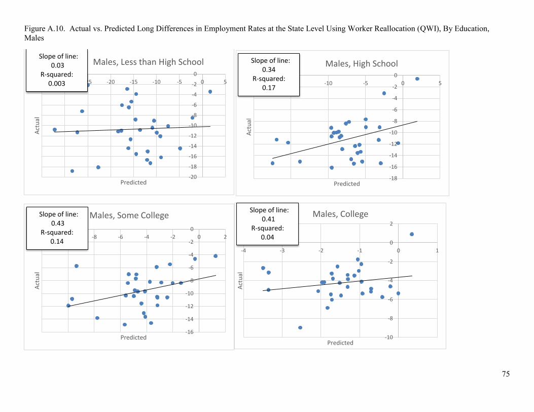
75

Figure A.10. Actual vs. Predicted Long Differences in Employment Rates at the State Level Using Worker Reallocation (QWI), By Education, Males

-20

-18

-16

-14

-12

-10

-8

-6

-4

-2

0

-35 -30 -25 -20 -15 -10 -5 0 5

Act

ual

Predicted

Males, Less than High SchoolSSlope of line:

0.03R-squared:

0.003

-18

-16

-14

-12

-10

-8

-6

-4

-2

0

-20 -15 -10 -5 0 5

Act

ual

Predicted

Males, High SchoolSSlope of line: 0.34

R-squared:0.17

-16

-14

-12

-10

-8

-6

-4

-2

0

-12 -10 -8 -6 -4 -2 0 2

Act

ual

Predicted

Males, Some CollegeSSlope of line:0.43

R-squared:0.14

-10

-8

-6

-4

-2

0

2

-4 -3 -2 -1 0 1

Act

ual

Predicted

Males, CollegeSSlope of line:0.41

R-squared:0.04

76

Figure A.11. Actual vs. Predicted Long Differences in Employment Rates at the State Level Using Worker Reallocation (QWI), By Education, Females

-25

-20

-15

-10

-5

0

5

-25 -20 -15 -10 -5 0

Act

ual

Predicted

Females, Less than High SchoolSSlope of line: -0.38

R-squared:0.08

-16

-14

-12

-10

-8

-6

-4

-2

0

-5 -4 -3 -2 -1 0

Act

ual

Predicted

Females, High SchoolSSlope of line:0.76

R-squared:0.08

-14

-12

-10

-8

-6

-4

-2

0

-12 -10 -8 -6 -4 -2 0

Act

ual

Predicted

Females, Some CollegeSSlope of line:

0.26R-squared:

0.08

-12

-10

-8

-6

-4

-2

0

2

-10 -8 -6 -4 -2 0A

ctu

al

Predicted

Females, CollegeSSlope of line: 0.06

R-squared:0.002

77

Figure A.12. Actual vs. Predicted Long Differences in Employment Rates at the State Level, By Education Groups and Sub-Periods (BDS job reallocation), Males

-20

-15

-10

-5

0

5

10

-25 -20 -15 -10 -5 0 5

Act

ual

Predicted

Males, Less than High SchoolSlope of fit line:0.32

R-squared:0.089

-20

-15

-10

-5

0

5

-25 -20 -15 -10 -5 0 5

Act

ual

Predicted

Males, High SchoolSlope of fit line:

0.45R-squared:

0.26

-20

-15

-10

-5

0

5

10

-20 -15 -10 -5 0 5 10

Act

ual

Predicted

Males, Some CollegeSlope of fit line: 0.85

R-squared:0.43

-10

-8

-6

-4

-2

0

2

4

-9 -7 -5 -3 -1 1 3 5

Act

ual

Predicted

Males, CollegeSlope of fit line: 0.69

R-squared:0.16

78

Figure A.13. Actual vs. Predicted Long Differences in Employment Rates at the State Level, By Education Groups and Sub-Periods (BDS job reallocation), Females

-20

-15

-10

-5

0

5

10

15

-25 -20 -15 -10 -5 0 5 10

Act

ual

Predicted

Females, Less than High SchoolSSlope of fit line: 0.71

R-squared:0.25

-15

-10

-5

0

5

10

-30 -25 -20 -15 -10 -5 0 5 10

Act

ual

Predicted

Females, High SchoolSSlope of fit line: 0.56

R-squared:0.40

-15

-10

-5

0

5

10

15

-15 -10 -5 0 5Act

ual

Predicted

Females, Some CollegeSSlope of fit line:1.29

R-squared:0.45

-10

-5

0

5

10

15

-9 -7 -5 -3 -1 1 3 5

Act

ual

Predicted

Females, CollegeSSlope of fit line: 0.97

R-squared:0.18

79

Figure A.14: Actual and Predicted Changes in Employment Rates from Changes in Fluidity (QWI Job Reallocation Rate), 1998-00 to 2010-11, Males

Notes: The predicted changes use the estimated coefficients from specifications relating employment rates to QWI job reallocation rates for the 1998-2011 period. Predicted changes use changes in fluidity measures at the national level. All other effects are held constant. No estimates are presented for Age<25 and College.

-35

-30

-25

-20

-15

-10

-5

0

5

<25 25-34 35-54 55+

Age Group

Less than High School

Actual Predicted

-35

-30

-25

-20

-15

-10

-5

0

5

<25 25-34 35-54 55+

Age Group

High School

Actual "Predicted"

-35

-30

-25

-20

-15

-10

-5

0

5

<25 25-34 35-54 55+

Age Group

Some College

Actual Predicted

-35

-30

-25

-20

-15

-10

-5

0

5

25-34 35-54 55+

Age Group

College

Actual Predicted

80

Figure A.15. Actual and Predicted Changes in Employment Rates from Changes in Fluidity (QWI Job Reallocation Rate), 1998-00 to 2010-11, Females

Notes: The predicted changes use the estimated coefficients from specifications relating employment rates to QWI job reallocation rates for the 1998-2011 period. Predicted changes use changes in fluidity measures at the national level. All other effects are held constant. No estimates are presented for Age<25 and College.

-35

-30

-25

-20

-15

-10

-5

0

5

<25 25-34 35-54 55+

Age Group

Less than High School

Actual Predicted

-35

-30

-25

-20

-15

-10

-5

0

5

<25 25-34 35-54 55+

Age Group

High School

Actual "Predicted"

-35

-30

-25

-20

-15

-10

-5

0

5

<25 25-34 35-54 55+

Age Group

Some College

Actual Predicted

-35

-30

-25

-20

-15

-10

-5

0

5

25-34 35-54 55+

Age Group

College

Actual Predicted

81

Figure A.16. Actual and Predicted Changes in Employment Rates from Changes in Fluidity (QWI Churn Rate), 1998-00 to 2010-11, Males

Notes: The predicted changes use the estimated coefficients from specifications relating employment rates to QWI churn rates for the 1998-2011 period. Predicted changes use changes in fluidity measures at the national level. All other effects are held constant. No estimates are presented for Age<25 and College.

-35

-30

-25

-20

-15

-10

-5

0

5

<25 25-34 35-54 55+

Age Group

Less than High School

Actual Predicted

-35

-30

-25

-20

-15

-10

-5

0

5

<25 25-34 35-54 55+

Age Group

High School

Actual "Predicted"

-35

-30

-25

-20

-15

-10

-5

0

5

<25 25-34 35-54 55+

Age Group

Some College

Actual Predicted

-35

-30

-25

-20

-15

-10

-5

0

5

25-34 35-54 55+

Age Group

College

Actual Predicted

82

Figure A.17. Actual and Predicted Changes in Employment Rates from Changes in Fluidity (QWI Churn Rate), 1998-00 to 2010-11, Females

Notes: The predicted changes use the estimated coefficients from specifications relating employment rates to QWI churn rates for the 1998-2011 period. Predicted changes use changes in fluidity measures at the national level. All other effects are held constant. No estimates are presented for Age<25 and College.

-35

-30

-25

-20

-15

-10

-5

0

5

10

<25 25-34 35-54 55+

Age Group

Less than High School

Actual Predicted

-35

-30

-25

-20

-15

-10

-5

0

5

10

<25 25-34 35-54 55+

Age Group

High School

Actual "Predicted"

-35

-30

-25

-20

-15

-10

-5

0

5

10

<25 25-34 35-54 55+

Age Group

Some College

Actual Predicted

-35

-30

-25

-20

-15

-10

-5

0

5

10

25-34 35-54 55+

Age Group

College

Actual Predicted

83

Figure A.18. Actual vs. Predicted Changes in Employment Rate from Changes in Fluidity (BDS Job Reallocation Rate), 1987-89 to 1999-01, Males

Notes: Predicted changes use the estimated coefficients from specifications relating employment rates to BDS job reallocation rates for the 1987-2009 period. Predicted changes use changes in fluidity measures at the national level. All other effects are held constant. No estimates are presented for Age<25 and College.

-5

0

5

10

<25 25-34 35-54 55+

Age Group

Less than High School

Actual Predicted

-5

0

5

10

<25 25-34 35-54 55+

Age Group

High School

Actual "Predicted"

-5

0

5

10

<25 25-34 35-54 55+

Age Group

Some College

Actual Predicted

-5

0

5

10

25-34 35-54 55+

Age Group

College

Actual Predicted

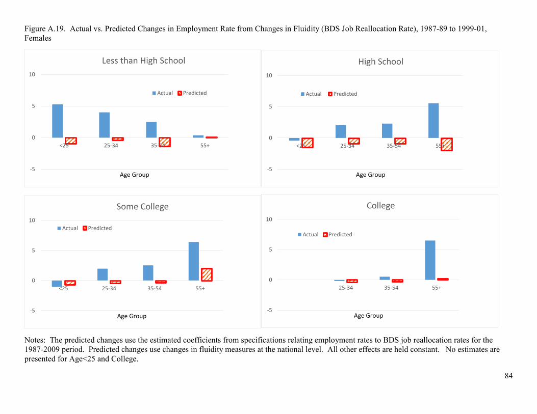
84

Figure A.19. Actual vs. Predicted Changes in Employment Rate from Changes in Fluidity (BDS Job Reallocation Rate), 1987-89 to 1999-01, Females

Notes: The predicted changes use the estimated coefficients from specifications relating employment rates to BDS job reallocation rates for the 1987-2009 period. Predicted changes use changes in fluidity measures at the national level. All other effects are held constant. No estimates are presented for Age<25 and College.

-5

0

5

10

<25 25-34 35-54 55+

Age Group

Less than High School

Actual Predicted

-5

0

5

10

<25 25-34 35-54 55+

Age Group

High School

Actual Predicted

-5

0

5

10

<25 25-34 35-54 55+

Age Group

Some College

Actual Predicted

-5

0

5

10

25-34 35-54 55+

Age Group

College

Actual Predicted

85

Figure A.20. Actual vs. Predicted Changes in Employment Rate from Changes in Fluidity (BDS Job Reallocation Rate), 1999-01 to 2008-10, Males

Notes: The predicted changes use the estimated coefficients from specifications relating employment rates to BDS job reallocation rates for the 1987-2009 period. Predicted changes use changes in fluidity measures at the national level. All other effects are held constant. No estimates are presented for Age<25 and College.

-20

-15

-10

-5

0

5

10

15

20

<25 25-34 35-54 55+

Age Group

Less than High School

Actual Predicted

-20

-15

-10

-5

0

5

10

15

20

<25 25-34 35-54 55+

Age Group

High School

Actual "Predicted"

-20

-15

-10

-5

0

5

10

15

20

<25 25-34 35-54 55+

Age Group

Some College

Actual Predicted

-20

-15

-10

-5

0

5

10

15

20

25-34 35-54 55+

Age Group

College

Actual Predicted

86

Figure A.21. Actual vs. Predicted Changes in Employment Rate from Changes in Fluidity (BDS Job Reallocation Rate), 1999-01 to 2008-10, Females

Notes: The predicted changes use the estimated coefficients from specifications relating employment rates to BDS job reallocation rates for the 1987-2009 period. Predicted changes use changes in fluidity measures at the national level. All other effects are held constant. No estimates are presented for Age<25 and College.

-20

-15

-10

-5

0

5

10

15

20

<25 25-34 35-54 55+

Age Group

Less than High School

Actual Predicted

-20

-15

-10

-5

0

5

10

15

20

<25 25-34 35-54 55+

Age Group

High School

Actual Predicted

-20

-15

-10

-5

0

5

10

15

20

<25 25-34 35-54 55+

Age Group

Some College

Actual Predicted

-20

-15

-10

-5

0

5

10

15

20

25-34 35-54 55+

Age Group

College

Actual Predicted

87

Appendix Tables

Table A.1 P-Values for Test of Overidentifying Restrictions for IV Results in Table 2

P-Values for IV Results Less than High

School High School

Some College

College

Males 0.22 0.78 0.51 0.82 Females 0.75 0.48 0.32 0.44

Table A.2 The Relationship Between Employment Rates and Labor Market Fluidity (Job reallocation Rates BDS), OLS and IV Results

OLS Results Less than High

School High School

Some College

College

Males 0.34 0.67 0.60 0.37 (0.16) (0.08) (0.10) (0.05) Females -0.35 0.12 0.09 0.13 (0.09) (0.09) (0.08) (0.04)

IV Results Less than High

School High School

Some College

College

Males 1.69 1.59 1.05 0.41 (0.49) (0.42) (0.25) (0.16) Females 1.61 1.98 0.84 0.45 (0.51) (0.48) (0.27) (0.28)

Notes: Standard errors clustered at the state level in parentheses. The dependent variable is the employment rate in the state-period-gender-education cell, and the measure of labor market fluidity is the BDS job reallocation rate. Control variables are state effects, the growth rate of national GDP, the deviation of national GDP from the Hodrick Prescott Trend, the Bartik-like control for state-level labor demand described in Appendix B, and controls for the number of children and young children in the household. The data are on a state by time period basis, where the time periods are 3-year non-overlapping periods from 1987-2010 (years running from April to March). Each cell in the above table reports coefficients from a separate regression for the indicated group. The fluidity measure (job reallocation rate) varies by state and time period. The regressions are employment-weighted using the average (over time) DHS denominator used to compute the fluidity measure. The instruments for the fluidity measure are the share of the working-age population in the state that is 18-24 and the first reallocation intensity instrument described in Appendix B (the IM instrument). No estimates are presented for Age<25 and College.

88

Table A.3 P-Values for Test of Overidentifying Restrictions for IV Results in Table A.2

P-Values for IV Results Less than High

School High School

Some College

College

Males 0.81 0.60 0.13 0.60 Females 0.54 0.65 0.00 0.54

Table A.4 P-Values for Test of Overidentifying Restrictions for IV Results in Table 3

Males, P-Values for IV Results Age Group

Less than High School

High School

Some College

College

<25 0.16 0.24 0.40

25-34 0.39 0.59 0.22 0.28

35-54 0.66 0.97 0.18 0.36

55+ 0.17 0.21 0.22 0.81

Females, P-Values for IV Results Age Group

Less than High School

High School

Some College

College

<25 0.28 0.46 0.38

25-34 0.21 0.24 0.92 0.99

35-54 0.37 0.77 0.82 0.09

55+ 0.25 0.21 0.61 0.44

89

Table A.5: The Relationship Between Employment Rates and Labor Market Fluidity (Worker Reallocation Rates), OLS Results

Males, OLS Results Age Group

Less than High School

High School

Some College

College

<25 0.46 0.33 0.33 (0.15) (0.10) (0.13) 25-34 0.33 0.17 0.22 0.09 (0.12) (0.09) (0.05) (0.06) 35-54 0.24 0.13 0.11 0.03 (0.10) (0.05) (0.03) (0.05) 55+ -0.10 0.08 -0.14 -0.18 (0.12) (0.10) (0.10) (0.09)

Females, OLS Results Age Group

Less than High School

High School

Some College

College

<25 0.42 0.26 0.37 (0.11) (0.09) (0.08) 25-34 0.21 0.08 0.26 0.10 (0.16) (0.12) (0.06) (0.09) 35-54 -0.02 0.02 0.03 0.06 (0.09) (0.06) (0.06) (0.05) 55+ -0.17 -0.09 -0.05 -0.23 (0.09) (0.09) (0.09) (0.16)

Notes: See Table 3 in the main text.

90

Table A.6 Implied Elasticities for Employment Rates and U-Pop Rates With Respect to Changes in Worker Reallocation Rates, Males

Males, Employment Rates Age Group

Less than High School

High School

Some College

College

<25 1.36 0.68 0.53 0.12 25-34 0.49 0.30 0.15 0.09 35-54 0.32 0.19 0.08 0.06 55+ 0.16 0.18 0.06 -0.05

Males, U-Pop Rates Age Group

Less than High School

High School

Some College

College

<25 -1.17 -2.22 -2.05 -2.12 25-34 -3.08 -2.61 -2.10 -2.37 35-54 -3.07 -3.14 -2.96 -3.32 55+ -3.11 -4.17 -1.71 -3.61 Notes: The top panel reports elasticities based on the estimates from Table 3. The bottom panel has the estimates based on Table A.7 below.

91

Table A.7: The Relationship Between U-Pop Rates and Labor Market Fluidity (Worker Reallocation Rates), IV Results

Males, IV Results Age Group

Less than High School

High School

Some College

College

<25 -0.29 -0.66 -0.35 (0.14) (0.32) (0.21) 25-34 -0.56 -0.49 -0.32 -0.24 (0.21) (0.30) (0.19) (0.16) 35-54 -0.43 -0.41 -0.35 -0.31 (0.17) (0.19) (0.17) (0.21) 55+ -0.22 -0.35 -0.16 -0.33 (0.08) (0.12) (0.11) (0.37)

Females, IV Results Age Group

Less than High School

High School

Some College

College

<25 -0.31 -0.16 -0.22 (0.17) (0.15) (0.12) 25-34 -0.15 -0.30 -0.29 -0.24 (0.09) (0.25) (0.19) (0.18) 35-54 -0.24 -0.27 -0.18 -0.15 (0.07) (0.12) (0.10) (0.09) 55+ -0.05 -0.24 -0.21 -0.24 (0.09) (0.10) (0.12) (0.25)

Notes: The specifications considered in this table are the same as in Table 3, except that the dependent variable is the U-Pop rate (ratio of unemployed persons to all persons in the group) rather than the employment rate. See notes to Table 3 for additional information.

92

Table A.8 P-Values for Test of Overidentifying Restrictions for IV Results in Table A.7

Males, P-Values for IV Results Age Group

Less than High School

High School

Some College

College

<25 0.10 0.19 0.39

25-34 0.12 0.16 0.41 0.28

35-54 0.07 0.50 0.09 0.21

55+ 0.17 0.18 0.61 0.47

Females, P-Values for IV Results Age Group

Less than High School

High School

Some College

College

<25 0.02 0.03 0.43

25-34 0.05 0.08 0.26 0.14

35-54 0.06 0.47 0.07 0.25

55+ 0.23 0.13 0.68 0.57

93

Table A.9: The Relationship Between Employment Rates and Labor Market Fluidity (Worker Reallocation Rate), Using 2 Year MA

IV Results (All Periods) Less than High

School High School

Some College

College

Males 0.72 0.65 0.56 0.33 (0.16) (0.39) (0.26) (0.16) Females 0.40 0.36 0.47 0.45 (0.09) (0.30) (0.21) (0.20)

IV Results (Outside the Great Recession) Less than High

School High School

Some College

College

Males 0.76 0.75 0.60 0.37 (0.12) (0.34) (0.19) (0.12) Females 0.41 0.41 0.59 0.56 (0.08) (0.21) (0.17) (0.15)

IV Results (During the Great Recession) Less than High

School High School

Some College

College

Males 1.43 1.10 0.99 0.62 (0.55) (0.87) (0.66) (0.57) Females 0.72 0.71 1.09 0.94 (0.35) (0.48) (0.49) (0.59)

IV Results (Pre-2007) Less than High

School High School

Some College

College

Males 0.46 0.49 0.48 0.29 (0.20) (0.36) (0.24) (0.17) Females 0.38 0.28 0.39 0.67 (0.16) (0.22) (0.18) (0.21)

IV Results (Post-2007) Less than High

School High School

Some College

College

Males 0.81 0.90 0.77 0.54 (0.41) (0.66) (0.50) (0.41) Females 0.56 0.62 0.70 0.90 (0.31) (0.35) (0.32) (0.49)

Notes: This table follows the measures, specifications and IV estimation in Table 2 except as follows: All variables are averages for 2-year non-overlapping time periods rather than 3-year periods. The second panel above considers a specification that allows the coefficient on the worker reallocation fluidity measure to differ freely between the 2008-09 Great Recession period and the rest of the sample. Specifically, the regression considers the same controls as in the top panel while

94

including GR*Worker Reallocation Rate and (1-GR)*Worker Reallocation Rate as explanatory variables, where GR=1 for the 2-year 2008-09 and 0 otherwise. It also includes the GR dummy variable entered separately as a regressor. The third panel adopts the same approach to allow the coefficient on the worker reallocation fluidity measure to differ freely before and after 2007, i.e., between the period that ends in 2006-07 and the periods 2008-09 and 2010-11. See notes to Table 2 for other details.

95

Appendix B: Description of Bartik-like (1991) measures used in the empirical analysis

We use three Bartik-like (1991) measures in Section IV. The first is a control for state-level

labor demand:

𝐿𝐷𝑠𝑡 = ∑ 𝜃𝑖𝑠𝑡𝑔𝑖𝑡~𝑠

𝑖

,

where 𝐿𝐷𝑠𝑡 varies by state s and time t , 𝜃𝑖𝑠𝑡 are Davis, Haltiwanger and Schuh (1996) (DHS)

employment weights for industry i in state s at time t, and 𝑔𝑖𝑡~𝑠 is the DHS net employment growth

rate at the “national” level for industry i at time t. DHS weights at the industry-state-time level are

the average of employment in t-1 and t in the industry and state divided by the average of

employment in t-1 and t in the state. By “national” we mean the weighted average employment

growth rate for all states excluding the own state s (so the ~𝑠 superscript refers to all states but s).

Our two Bartik-like instruments capture changes over time in state-level reallocation

intensities that derive from “national” changes in the industry mix of employment and the industry-

level reallocation intensities. Our first state-level reallocation intensity instrument is

𝐼𝑀𝑠𝑡 = ∑ 𝜃𝑖𝑠𝑡−1𝑔𝑖𝑡~𝑠

𝑖

𝐽𝑅𝑖𝑡~𝑠,

where 𝐽𝑅𝑖𝑡~𝑠 is the “national” job reallocation rate for industry i at time t, excluding the own state

contribution to job reallocation. Here, we use lagged industry-level DHS employment weights in the

state, since we use this variable as an instrument rather than a control. Our second reallocation

intensity instrument is

𝐼𝑀2𝑠𝑡 = ∑ 𝜃𝑖𝑠𝑡−1

𝑖

𝐽𝑅𝑖𝑡~𝑠

These two measures are clearly related, but they capture somewhat different variation. The

second reallocation intensity instrument captures the interaction between the industry-level

reallocation intensities in other states (the 𝐽𝑅𝑖𝑡~𝑠 terms) and the state’s own legacy industry structure

(the 𝜃𝑖𝑠𝑡−1 industry employment shares). The first reallocation intensity instrument also includes

96

changes in the national industry mix of employment (the 𝑔𝑖𝑡~𝑠) as part of the term that interacts with

the state’s legacy industry structure. When we use these reallocation intensity instruments, we

always include controls for the Bartik-like labor demand measure defined above and all other

controls discussed in the main text. Thus, our IV estimation with the reallocation intensity

instruments relies on variation in 𝐼𝑀𝑠𝑡 and 𝐼𝑀2𝑠𝑡 conditional on 𝐿𝐷𝑠𝑡 and other controls to achieve

identification of the fluidity effects.

In constructing the three Bartik-like measures, we proceed as follows. First, we average the

quarterly QWI state-industry data on employment shares, growth rates and reallocation rates to the

annual level for the retimed years defined above. (The BDS state-industry data come to us at the

annual level for retimed years.) Second, we construct the “national” measures for each state and

year. Third, we construct annual versions of the three Bartik-like measures defined in this

appendix. Finally, we average these measures to the non-overlapping three-year periods used in the

regression analysis.