Lab 2b: Dynamic Response of a Rotor with Shaft Imbalance OBJECTIVE: • To calibrate an induction displacement sensor using a micrometer • To calculate and measure the natural frequency of a simply-supported shaft with a centered

load and compare the two frequencies • To balance an unbalanced rotating shaft using induction sensors and oscilloscope • To study changes rotor mass position affects the natural frequency • To study how adding a second rotor mass affects the system vibrational modes • To perform a frequency analysis on accelerometer data using a Fast Fourier Transform (FFT)

Figure 1: Bently Nevada RK 4 Rotor Kit Experimental Setup

PROCEDURE: DAY 1 – Sensor Calibration and Natural Frequency 1) You will calibrate the Proximity Induction Sensor 1 using the micrometer mounted to the

rotor test stand with a stainless steel washer mounted to the end of it. You will position the sensor in the upwards direction through the bottom of the bracket. The end result will be an equation that converts the induction sensor voltage to the distance between the steel and the sensor surface.

1

a) Unscrew and unplug the sensor from the Probe 1 input on the back of the Rotor Kit Proximitor Assembly (RKPA). Refer to Figure 1.

b) Unscrew the Induction Proximity Sensor 1 from the shaft imbalance bracket. Be sure to perform Step (a) first to avoid twisting the cord.

c) Drop the plug-end of the sensor from the RKPA through either of the lower holes of the

test stand bracket.

d) Carefully screw the induction sensor into an upper bracket hole that is directly inline with the lower hole in Step (c). Then re-attach the plug into the RKPA. Refer to Figure 2.

e) Position the sensor flush (as close as possible) with the steel washer mounted on the end

of the micrometer. Screw the sensor into the bracket and lowering the micrometer until the washer is touching the sensor. Refer to Figure 3. Screw the plug end of the induction sensor back into Port 1 of the RKPA.

f) Ensure that the output of Prox 1 on the front of the RKPA is connected to Channel 1 of the oscilloscope.

g) The micrometer reading while the wash is flush will be treated as the “zero point”. Once the system is powered, the voltage output at this zero point will be at a minimum. Likewise, voltage will stop increasing once the maximum range of the sensor is reached. These points represent the maximum range of the sensor.

Figure 2: Inserting the induction sensor plug-end into the calibration setup

2

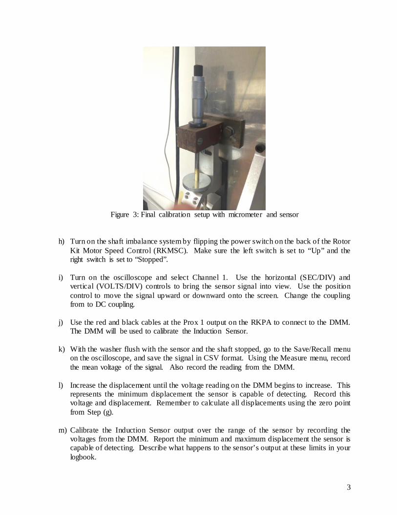
Figure 3: Final calibration setup with micrometer and sensor

h) Turn on the shaft imbalance system by flipping the power switch on the back of the Rotor

Kit Motor Speed Control (RKMSC). Make sure the left switch is set to “Up” and the right switch is set to “Stopped”.

i) Turn on the oscilloscope and select Channel 1. Use the horizontal (SEC/DIV) and vertical (VOLTS/DIV) controls to bring the sensor signal into view. Use the position control to move the signal upward or downward onto the screen. Change the coupling from to DC coupling.

j) Use the red and black cables at the Prox 1 output on the RKPA to connect to the DMM. The DMM will be used to calibrate the Induction Sensor.

k) With the washer flush with the sensor and the shaft stopped, go to the Save/Recall menu

on the oscilloscope, and save the signal in CSV format. Using the Measure menu, record the mean voltage of the signal. Also record the reading from the DMM.

l) Increase the displacement until the voltage reading on the DMM begins to increase. This

represents the minimum displacement the sensor is capable of detecting. Record this voltage and displacement. Remember to calculate all displacements using the zero point from Step (g).

m) Calibrate the Induction Sensor output over the range of the sensor by recording the voltages from the DMM. Report the minimum and maximum displacement the sensor is capable of detecting. Describe what happens to the sensor’s output at these limits in your logbook.

3

n) Using upscale/downscale progression, repeat the calibration runs so that you have five sets of data from which you can determine sensor bias and precision errors.

o) Unplug the sensor from the back of the RKPA, and remove it from the calibration

bracket. Replace the sensor in the shaft imbalance setup and plug it back into the RKPA. Disconnect and turn off the DMM.

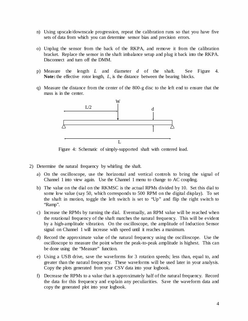
p) Measure the length L and diameter d of the shaft. See Figure 4.

Note: the effective rotor length, L, is the distance between the bearing blocks.

q) Measure the distance from the center of the 800-g disc to the left end to ensure that the mass is in the center.

Figure 4: Schematic of simply-supported shaft with centered load.

2) Determine the natural frequency by whirling the shaft.

a) On the oscilloscope, use the horizontal and vertical controls to bring the signal of Channel 1 into view again. Use the Channel 1 menu to change to AC coupling.

b) The value on the dial on the RKMSC is the actual RPMs divided by 10. Set this dial to some low value (say 50, which corresponds to 500 RPM on the digital display). To set the shaft in motion, toggle the left switch is set to “Up” and flip the right switch to “Ramp”.

c) Increase the RPMs by turning the dial. Eventually, an RPM value will be reached when the rotational frequency of the shaft matches the natural frequency. This will be evident by a high-amplitude vibration. On the oscilloscope, the amplitude of Induction Sensor signal on Channel 1 will increase with speed until it reaches a maximum.

d) Record the approximate value of the natural frequency using the oscilloscope. Use the oscilloscope to measure the point where the peak-to-peak amplitude is highest. This can be done using the “Measure” function.

e) Using a USB drive, save the waveforms for 3 rotation speeds; less than, equal to, and greater than the natural frequency. These waveforms will be used later in your analysis. Copy the plots generated from your CSV data into your logbook.

f) Decrease the RPMs to a value that is approximately half of the natural frequency. Record the data for this frequency and explain any peculiarities. Save the waveform data and copy the generated plot into your logbook.

W L/2

L

d

4

g) On the RKMSC, flip the left switch to “Down” and the right switch to “Stopped” and turn off the RKMSC.

h) Using an allen wrench loosen the screw on the side of the rotor mass, and slide the mass

approximately 1” from the bracket on the left side of the mass.

i) Turn the RKMSC back on and repeat Steps E thru I to observe the effect of the change in mass location on the natural frequency.

j) Replace the rotor mass to its original location by using the allen wrench to loosen the

screw and sliding the rotor mass to the 50% mark.

DAY 1 ANALYSIS 1) Create the calibration curve for the induction sensor. Construct a calibration curve including

the curve equation with the induction sensor voltage measurements on the x-axis (independent) and the micrometer measurements on the y-axis (dependent). This curve will be used to convert the voltage to a distance between the shaft and proximity sensor.

2) Determine error in calibration curve using standard error of the fit and confidence intervals. 3) Calculate the theoretical natural frequency of the simply-supported shaft with a centered load

using Appendix A. Compare this with the measured value of natural frequency and discuss possible reasons for the difference.

4) Compare the center-load natural frequency to the frequency obtained when the rotor mass

was shifted to the left. If the natural frequency is different, explain why the frequency differs and why it is either higher or lower.

5

DAY 2 – SHAFT BALANCING, MODES, FREQUENCY ANALYSIS 1) Note: in these steps you will use voltage as a measure of vibration. This is done to save time

by eliminating the need to convert from voltage to deflection.

a) Ensure Induction Sensor 1 is connected to Channel 1 on the oscilloscope. b) Using a BNC coaxial cable, connect the channel labeled Kφ on the RKPA front panel to

Channel 2 of the oscilloscope. This channel represents a second induction sensor that detects a notch located on the shaft (Induction Sensor 2 in Figure 1). This sensor can be used to determine the rotational speed of the shaft without using the RPM display.

c) Use the Channel 2 menu to set the coupling to AC. Use the horizontal and vertical controls to bring both Channel 1 and Channel 2 into view on the oscilloscope screen.

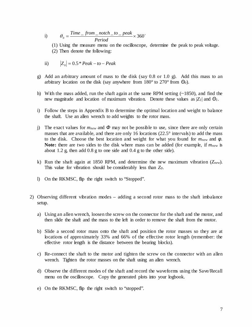
d) Rotate the shaft with a single, centered rotor mass (no weights added) at a speed setting of approximately 1850 RPM. Channel 1 should look like a sine wave, and Channel 2 will be flat except when the sensor detects the notch. At that point there will be a large dip in the signal, as shown in Figure 5.

e) Use the Measure function on Channel 1 to determine the period of the vibration of the shaft. Next, push the Run/Stop button to freeze the signal displays. Use the cursors to determine the time between the notch and the maximum vibration (max voltage) in the shaft. This is illustrated in Figure 5.

Figure 5: Plot showing method of determining location of maximum vibration

f) Determine where on the disk the maximum vibration takes place. The location is defined

by an angle Θ0. This angle can be found using this equation:

6

i) 360____0 ×=

PeriodpeaktonotchfromTimeθ

(1) Using the measure menu on the oscilloscope, determine the peak to peak voltage. (2) Then denote the following:

ii) PeaktoPeakZ −−= *5.00

g) Add an arbitrary amount of mass to the disk (say 0.8 or 1.0 g). Add this mass to an arbitrary location on the disk (say anywhere from 180° to 270° from Θ0).

h) With the mass added, run the shaft again at the same RPM setting (~1850), and find the new magnitude and location of maximum vibration. Denote these values as |Z1| and Θ1.

i) Follow the steps in Appendix B to determine the optimal location and weight to balance the shaft. Use an allen wrench to add weights to the rotor mass.

j) The exact values for mnew and Φ may not be possible to use, since there are only certain masses that are available, and there are only 16 locations (22.5° intervals) to add the mass to the disk. Choose the best location and weight for what you found for mnew and φ. Note: there are two sides to the disk where mass can be added (for example, if mnew is about 1.2 g, then add 0.8 g to one side and 0.4 g to the other side).

k) Run the shaft again at 1850 RPM, and determine the new maximum vibration (Znew). This value for vibration should be considerably less than Z0.

l) On the RKMSC, flip the right switch to “Stopped”.

2) Observing different vibration modes – adding a second rotor mass to the shaft imbalance

setup. a) Using an allen wrench, loosen the screw on the connector for the shaft and the motor, and

then slide the shaft and the mass to the left in order to remove the shaft from the motor.

b) Slide a second rotor mass onto the shaft and position the rotor masses so they are at locations of approximately 33% and 66% of the effective rotor length (remember: the effective rotor length is the distance between the bearing blocks).

c) Re-connect the shaft to the motor and tighten the screw on the connector with an allen

wrench. Tighten the rotor masses on the shaft using an allen wrench.

d) Observe the different modes of the shaft and record the waveforms using the Save/Recall menu on the oscilloscope. Copy the generated plots into your logbook.

e) On the RKMSC, flip the right switch to “stopped”.

7

f) Remove the second rotor mass and replace the original rotor mass to its original location by using the allen wrench to loosen the screws.

3) Frequency analysis

a) Turn on the oscilloscope and connect the accelerometer output to Channel 1. b) Turn on the RKMSC and set the speed 1850 RPM. c) Allow sensor signal and shaft speed to stabilize and then push the Run/Stop button. Save

the waveforms for both signals in CSV format to a USB drive. d) The FFT, or Fast Fourier Transform, is an algorithm that is used in frequency analysis to

identify the operational frequencies of a system. Using a computer program of your choice, perform an FFT analysis on your data from Step (c) to determine which frequencies are present in the system. There may be several frequencies (i.e. the shaft frequency, the motor frequency, the bearing frequency). Copy the plot of the waveform data into your logbook.

DAY 2 ANALYSIS 1) Convert the Induction Sensor voltage into deflection using the calibration curves you found

in the Day 1 Analysis section. Plot the data as one smooth signal. 2) Convert the voltage values of Z0 and Znew into deflection using the calibration curve.

Comment on how well the mass balancing worked on reducing the vibration. Also, if reduced vibration remained, discuss reasons why and any effect of signal noise on the results.

3) Note the different modes of vibration when a second rotor mass is added to the assembly.

Record the natural frequencies. 4) Perform a frequency analysis on the accelerometer data using a computer program of your

choice with a Fast Fourier Transform (FFT) function.

8

APPENDIX A: NATURAL FREQUENCY OF A SIMPLY-SUPPORTED SHAFT WITH CENTERED LOAD The natural frequency of a simply-supported shaft with a centered load is

stn x

gω∆

=

where g is the gravitational acceleration (= 9.806 m/s2) and .

EI

WLxst 48

3

=∆

where W is the weight of the centered mass (m = 800 g), L is the length of the shaft, E is the modulus of elasticity (207 GPa), and I is the moment of inertia of the shaft (= πd4/64).

9

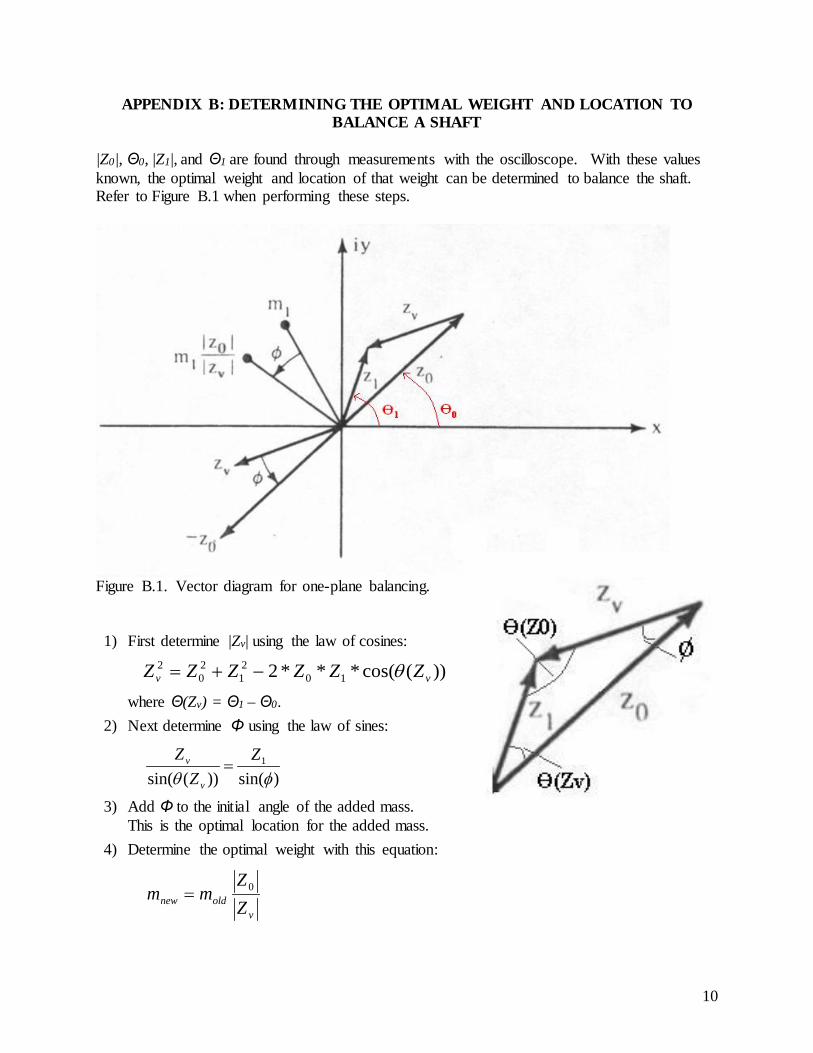
APPENDIX B: DETERMINING THE OPTIMAL WEIGHT AND LOCATION TO BALANCE A SHAFT

|Z0|, Θ0, |Z1|, and Θ1 are found through measurements with the oscilloscope. With these values known, the optimal weight and location of that weight can be determined to balance the shaft. Refer to Figure B.1 when performing these steps.

Figure B.1. Vector diagram for one-plane balancing. 1) First determine |Zv| using the law of cosines:

))(cos(***2 102

120

2vv ZZZZZZ θ−+=

where Θ(Zv) = Θ1 – Θ0.

2) Next determine Φ using the law of sines:

)sin())(sin(

1

φθZ

ZZ

v

v =

3) Add Φ to the initial angle of the added mass. This is the optimal location for the added mass.

4) Determine the optimal weight with this equation:

v

oldnew ZZ

mm 0=

10

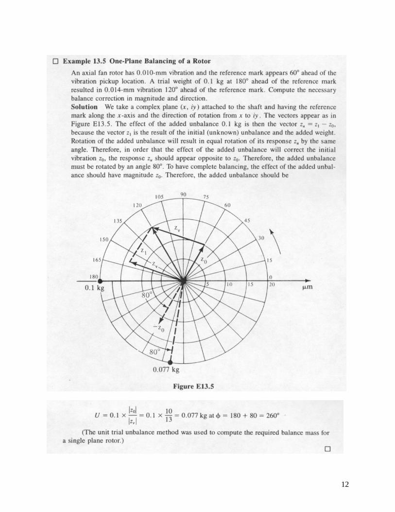
APPENDIX C: ADDITIONAL INFORMATION AND EXAMPLE ON SHAFT

BALANCING

11

12