la b basic modeling concepts - brawijaya...

Harrell−Ghosh−Bowden: Simulation Using ProModel, Second Edition

II. Labs 7. Basic Modeling Concepts

© The McGraw−Hill Companies, 2004

L A B

7 BASIC MODELINGCONCEPTS

465

Imagination is more important than knowledge.—Albert Einstein

In this chapter we continue to describe other basic features and modeling conceptsof ProModel. In Section L7.1 we show an application with multiple locations andmultiple entity types. Section L7.2 describes modeling of multiple parallel loca-tions. Section L7.3 shows various routing rules. In Section L7.4 we introduce theconcept of variables. Section L7.5 introduces the inspection process, tracking of de-fects, and rework. In Section L7.6 we show how to assemble nonidentical entitiesand produce assemblies. In Section L7.7 we show the process of making temporaryentities through the process of loading and subsequent unloading. Section L7.8describes how entities can be accumulated before processing. Section L7.9 showsthe splitting of one entity into multiple entities. In Section L7.10 we introducevarious decision statements with appropriate examples. Finally, in Section L7.11we show you how to model a system that shuts down periodically.

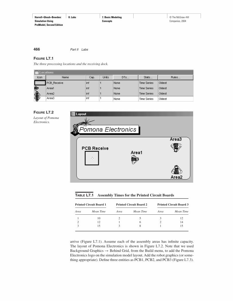
L7.1 Multiple Locations, Multiple Entity TypesProblem StatementIn one department at Pomona Electronics, three different printed circuit boardsare assembled. Each board is routed through three assembly areas. The routingorder is different for each of the boards. Further, the time to assemble a board de-pends on the board type and the operation. The simulation model is intended todetermine the time to complete 500 boards of each type. The assembly time foreach board is exponentially distributed with the mean times shown in Table L7.1.

Define three locations (Area1, Area2, and Area3) where assembly work isdone and another location, PCB_Receive, where all the printed circuit boards




466 Part II Labs

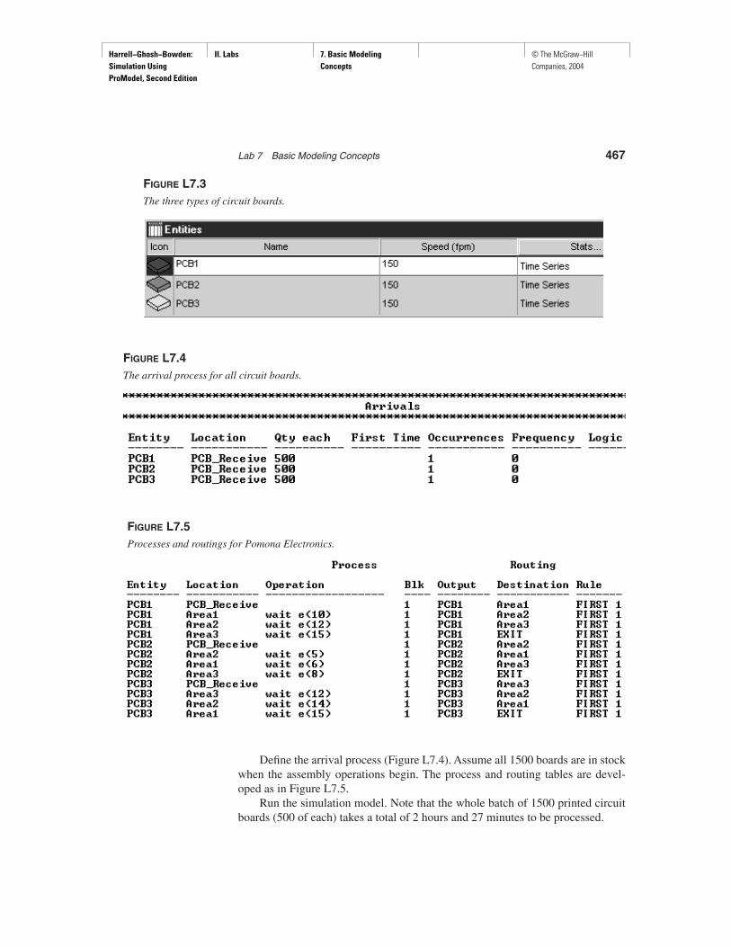
arrive (Figure L7.1). Assume each of the assembly areas has infinite capacity.The layout of Pomona Electronics is shown in Figure L7.2. Note that we usedBackground Graphics → Behind Grid, from the Build menu, to add the PomonaElectronics logo on the simulation model layout. Add the robot graphics (or some-thing appropriate). Define three entities as PCB1, PCB2, and PCB3 (Figure L7.3).

TABLE L7.1 Assembly Times for the Printed Circuit Boards

Printed Circuit Board 1 Printed Circuit Board 2 Printed Circuit Board 3

Area Mean Time Area Mean Time Area Mean Time

1 10 2 5 3 122 12 1 6 2 143 15 3 8 1 15

FIGURE L7.1The three processing locations and the receiving dock.

FIGURE L7.2Layout of PomonaElectronics.




Lab 7 Basic Modeling Concepts 467

Define the arrival process (Figure L7.4). Assume all 1500 boards are in stockwhen the assembly operations begin. The process and routing tables are devel-oped as in Figure L7.5.

Run the simulation model. Note that the whole batch of 1500 printed circuitboards (500 of each) takes a total of 2 hours and 27 minutes to be processed.

FIGURE L7.3The three types of circuit boards.

FIGURE L7.5Processes and routings for Pomona Electronics.

FIGURE L7.4The arrival process for all circuit boards.




468 Part II Labs

L7.2 Multiple Parallel Identical LocationsLocation: Capacity versus UnitsEach location in a model has associated with it some finite capacity. The capacityof a location refers to the maximum number of entities that the location can holdat any time. The reserved word INF or INFINITE sets the capacity to the maximumallowable value. The default capacity for a location is one unless a counter, con-veyor, or queue is the first graphic assigned to it. The default capacity in that caseis INFINITE.

The number of units of a location refers to the number of identical, inter-changeable, and parallel locations referenced as a single location for routing andprocessing. A multiunit location eliminates the need to create multiple locationsand multiple processes for locations that do the same thing. While routings to andfrom each unit are the same, each unit may have unique downtimes.

A multiunit location is created by entering a number greater than one as thenumber of units for a normal location. A corresponding number of locations willappear below the original location with a numeric extension appended to eachcopied location name designating the unit number of that location. The originallocation record becomes the prototype for the unit records. Each unit will inheritthe prototype’s characteristics unless the individual unit’s characteristics arechanged. Downtimes, graphic symbols, and, in the case of multicapacity loca-tions, capacities may be assigned to each unit. As the number of units of a locationis changed, the individual unit locations are automatically created or destroyedaccordingly.

The following three situations describe the advantages and disadvantages ofmodeling multicapacity versus multiunit locations.

• Multicapacity locations. Locations are modeled as a single unit withmulticapacity (Figure L7.6). All elements of the location performidentical operations. When one element of the location is unavailable dueto downtime, all elements are unavailable. Only clock-based downtimesare allowed.

• Multiunit locations. Locations are modeled as single capacity but multipleunits (Figure L7.7). These are locations consisting of two or more paralleland interchangeable processing units. Each unit shares the same sources ofinput and the same destinations for output, but each may have independentoperating characteristics. This method provides more flexibility in theassignment of downtimes and in selecting an individual unit to process aparticular entity.

• Multiple, single-capacity locations. Locations are modeled as individualand single capacity (Figure L7.8). Usually noninterchangeable locationsare modeled as such. By modeling as individual locations, we gain theflexibility of modeling separate downtimes for each element. In addition,we now have complete flexibility to determine which element willprocess a particular entity.





Problem StatementAt San Dimas Electronics, jobs arrive at three identical inspection machines ac-cording to an exponential distribution with a mean interarrival time of 12 minutes.The first available machine is selected. Processing on any of the parallel machinesis normally distributed with a mean of 10 minutes and a standard deviation of3 minutes. Upon completion, all jobs are sent to a fourth machine, where theyqueue up for date stamping and packing for shipment; this takes five minutes nor-mally distributed with a standard deviation of two minutes. Completed jobs thenleave the system. Run the simulation for one month (20 days, eight hours each).Calculate the average utilization of the four machines. Also, how many jobs areprocessed by each of the four machines?

Define a location called Inspect. Change its units to 3. Three identical parallellocations—that is, Inspect.1, Inspect.2, and Inspect.3—are thus created. Also, de-fine a location for all the raw material to arrive (Material_Receiving). Change thecapacity of this location to infinite. Define a location for Packing (Figure L7.9).Select Background Graphics from the Build menu. Make up a label “San DimasElectronics.” Add a rectangular border. Change the font and color appropriately.

FIGURE L7.7Multiple units of single-capacity locations.

FIGURE L7.8Multiple single-capacity locations.

FIGURE L7.6Single unit of multicapacity location.




470 Part II Labs

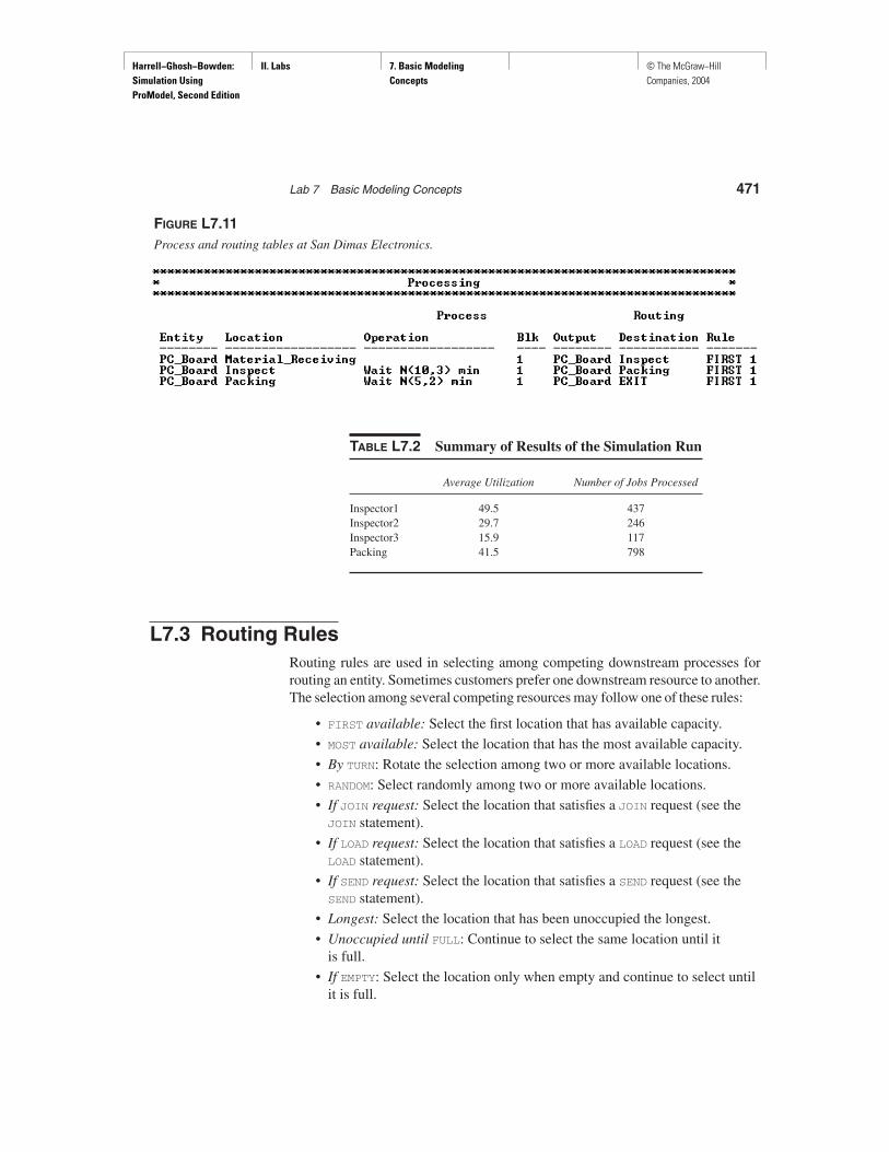
Define an entity called PCB. Define the frequency of arrival of the entity PCBas exponential with a mean interarrival time of 12 minutes (Figure L7.10). Definethe process and routing at San Dimas Electronics as shown in Figure L7.11.

In the Simulation menu select Options. Enter 160 in the Run Hours box. Runthe simulation model. The average utilization and the number of jobs processed atthe four locations are given in Table L7.2.

FIGURE L7.9The locations and the layout of San Dimas Electronics.

FIGURE L7.10Arrivals of PCB at San Dimas Electronics.





FIGURE L7.11Process and routing tables at San Dimas Electronics.

TABLE L7.2 Summary of Results of the Simulation Run

Average Utilization Number of Jobs Processed

Inspector1 49.5 437Inspector2 29.7 246Inspector3 15.9 117Packing 41.5 798

L7.3 Routing RulesRouting rules are used in selecting among competing downstream processes forrouting an entity. Sometimes customers prefer one downstream resource to another.The selection among several competing resources may follow one of these rules:

• FIRST available: Select the first location that has available capacity.

• MOST available: Select the location that has the most available capacity.

• By TURN: Rotate the selection among two or more available locations.

• RANDOM: Select randomly among two or more available locations.

• If JOIN request: Select the location that satisfies a JOIN request (see theJOIN statement).

• If LOAD request: Select the location that satisfies a LOAD request (see theLOAD statement).

• If SEND request: Select the location that satisfies a SEND request (see theSEND statement).

• Longest: Select the location that has been unoccupied the longest.

• Unoccupied until FULL: Continue to select the same location until itis full.

• If EMPTY: Select the location only when empty and continue to select untilit is full.




472 Part II Labs

• Probabilistic: Select based on the probability specified (such as .75).

• User condition: Select the location that satisfies the Boolean conditionspecified by the user (such as AT2>5). Conditions may include anynumeric expression except for location attributes, resource-specificfunctions, and downtime-specific functions.

• CONTINUE: Continue at the same location for additional operations.CONTINUE is allowed only for blocks with a single routing.

• As ALTERNATE to: Select as an alternate if available and if none of theabove rules can be satisfied.

• As BACKUP: Select as a backup if the location of the first preference is down.

• DEPENDENT: Select only if the immediately preceding routing was processed.

If only one routing is defined for a routing block, use the first available, join, load,send, if empty, or continue rule. The most available, by turn, random, longest un-occupied, until full, probabilistic, and user condition rules are generally only use-ful when a block has multiple routings.

Problem StatementAmar, Akbar, and Anthony are three tellers in the local branch of Bank of India.Figure L7.12 shows the layout of the bank. Assume that customers arrive at thebank according to a uniform distribution (mean of five minutes and half-width offour minutes). All the tellers service the customers according to another uniform

FIGURE L7.12Layout of the Bank ofIndia.





FIGURE L7.14Queue menu.

FIGURE L7.13Locations at the Bank of India.

distribution (mean of 10 minutes and half-width of 6 minutes). However, the cus-tomers preferAmar toAkbar, andAkbar overAnthony. If the teller of choice is busy,the customers choose the first available teller. Simulate the system for 200 customerservice completions. Estimate the teller’s utilization (percentage of time busy).

The locations are defined as Akbar, Anthony, Amar, Teller_Q, and Enter asshown in Figure L7.13. The Teller_Q is exactly 100 feet long. Note that we havechecked the queue option in the Conveyor/Queue menu (Figure L7.14). The




474 Part II Labs

customer arrival process is shown in Figure L7.15. The processes and routings areshown in Figure L7.16. Note that the customers go to the tellers Amar, Akbar, andAnthony in the order they are specified in the routing table.

The results of the simulation model are shown in Table L7.3. Note that Amar,being the favorite teller, is much more busy than Akbar and Anthony.

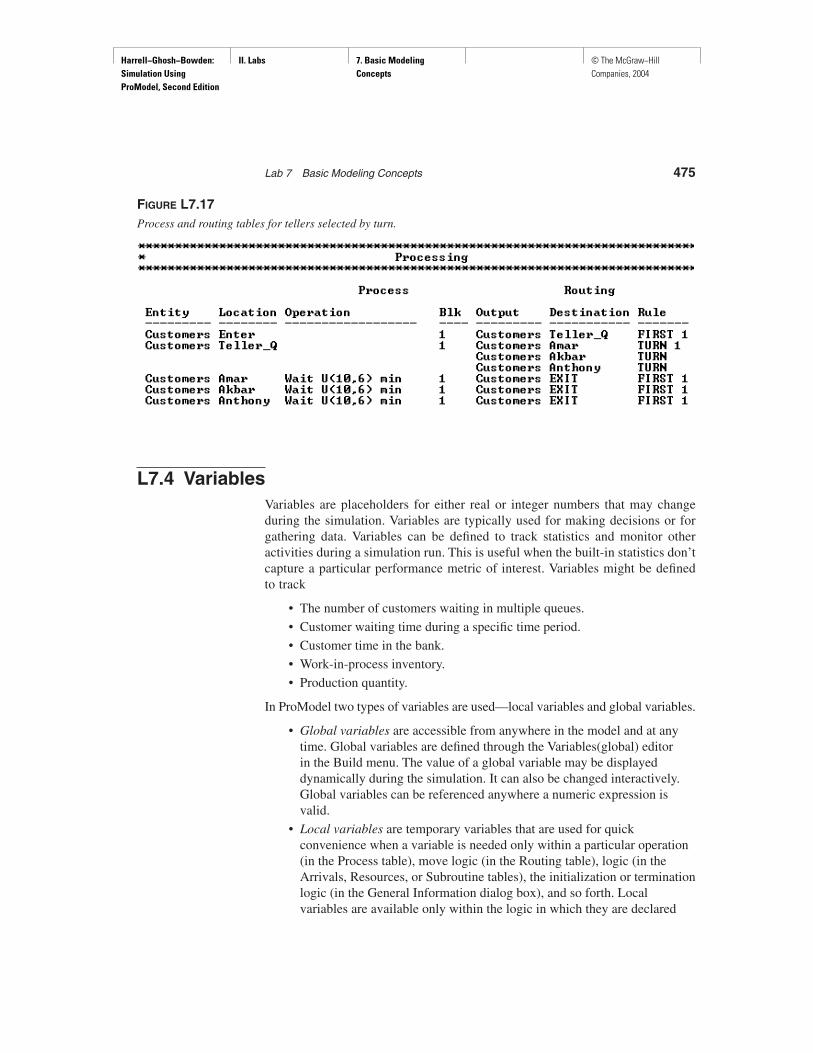
If the customers were routed to the three tellers in turn (selected in rotation),the process and routing tables would be as in Figure L7.17. Note that By Turn wasselected from the Rule menu in the routing table. These results of the simulationmodel are also shown in Table L7.3. Note that Amar, Akbar, and Anthony are nowutilized almost equally.

FIGURE L7.15Customer arrival at the Bank of India.

FIGURE L7.16Process and routing tables at the Bank of India.

TABLE L7.3 Utilization of Tellers at the Bank of India

% Utilization

Selection in Order Selection byTellers of Preference Turn

Amar 79 63.9Akbar 64.7 65.1Anthony 46.9 61.5





L7.4 VariablesVariables are placeholders for either real or integer numbers that may changeduring the simulation. Variables are typically used for making decisions or forgathering data. Variables can be defined to track statistics and monitor otheractivities during a simulation run. This is useful when the built-in statistics don’tcapture a particular performance metric of interest. Variables might be definedto track

• The number of customers waiting in multiple queues.

• Customer waiting time during a specific time period.

• Customer time in the bank.

• Work-in-process inventory.

• Production quantity.

In ProModel two types of variables are used—local variables and global variables.

• Global variables are accessible from anywhere in the model and at anytime. Global variables are defined through the Variables(global) editorin the Build menu. The value of a global variable may be displayeddynamically during the simulation. It can also be changed interactively.Global variables can be referenced anywhere a numeric expression isvalid.

• Local variables are temporary variables that are used for quickconvenience when a variable is needed only within a particular operation(in the Process table), move logic (in the Routing table), logic (in theArrivals, Resources, or Subroutine tables), the initialization or terminationlogic (in the General Information dialog box), and so forth. Localvariables are available only within the logic in which they are declared

FIGURE L7.17Process and routing tables for tellers selected by turn.




476 Part II Labs

and are not defined in the Variables edit table. They are created for eachentity, downtime occurrence, or the like executing a particular section oflogic. A new local variable is created for each entity that encounters anINT or REAL statement. It exists only while the entity processes the logicthat declared the local variable. Local variables may be passed tosubroutines as parameters and are available to macros.

A local variable must be declared before it is used. To declare a local variable,use the following syntax:

INT or REAL <name1>{= expression}, <name2>{= expression}

Examples:

INT HourOfDay, WIPREAL const1 = 2.5, const2 = 5.0INT Init_Inventory = 170

In Section L7.11 we show you how to use a local variable in your simulationmodel logic.

Problem Statement—Tracking Work in Process and ProductionIn the Poly Casting Inc. machine shop, raw castings arrive in batches of fourevery hour. From the raw material store they are sent to the mill, where they un-dergo a milling operation that takes an average of three minutes with a standarddeviation of one minute (normally distributed). The milled castings go to thegrinder, where they are ground for a duration that is uniformly distributed (mini-mum four minutes and maximum six minutes) or U(5,1). After grinding, theground pieces go to the finished parts store. Run the simulation for 100 hours.Track the work-in-process inventory and the production quantity.

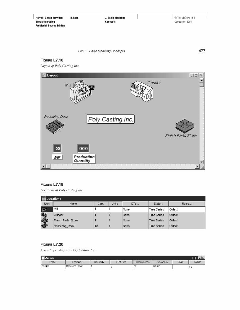
The complete simulation model layout is shown in Figure L7.18. The loca-tions are defined as Receiving_Dock, Mill, Grinder, and Finish_Parts_Store(Figure L7.19). Castings (entity) are defined to arrive in batches of four (Qtyeach) every 60 minutes (Frequency) as shown in Figure L7.20. The processes androutings are shown in Figure L7.21.

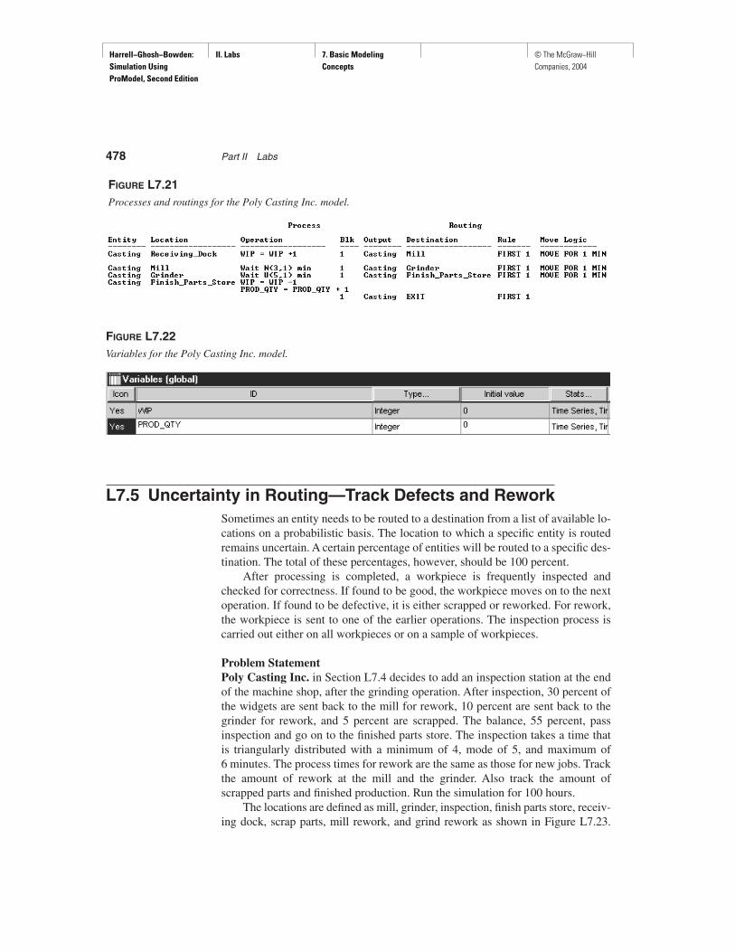
Define a variable in your model to track the work-in-process inventory (WIP)of parts in the machine shop. Also define another variable to track the production(PROD_QTY) of finished parts (Figure L7.22). Note that both of these are integertype variables.

In the process table, add the following operation statement in the Receivinglocation (Figure L7.21).

WIP = WIP + 1

Add the following operation statements in the outgoing Finish_Parts_Store loca-tion (Figure L7.21):

WIP = WIP - 1PROD_QTY = PROD_QTY + 1

Alternatively, these three statements could be written as INC WIP, DEC WIP, andINC PROD_QTY.





FIGURE L7.18Layout of Poly Casting Inc.

FIGURE L7.19Locations at Poly Casting Inc.

FIGURE L7.20Arrival of castings at Poly Casting Inc.




478 Part II Labs

L7.5 Uncertainty in Routing—Track Defects and ReworkSometimes an entity needs to be routed to a destination from a list of available lo-cations on a probabilistic basis. The location to which a specific entity is routedremains uncertain. A certain percentage of entities will be routed to a specific des-tination. The total of these percentages, however, should be 100 percent.

After processing is completed, a workpiece is frequently inspected andchecked for correctness. If found to be good, the workpiece moves on to the nextoperation. If found to be defective, it is either scrapped or reworked. For rework,the workpiece is sent to one of the earlier operations. The inspection process iscarried out either on all workpieces or on a sample of workpieces.

Problem StatementPoly Casting Inc. in Section L7.4 decides to add an inspection station at the endof the machine shop, after the grinding operation. After inspection, 30 percent ofthe widgets are sent back to the mill for rework, 10 percent are sent back to thegrinder for rework, and 5 percent are scrapped. The balance, 55 percent, passinspection and go on to the finished parts store. The inspection takes a time thatis triangularly distributed with a minimum of 4, mode of 5, and maximum of6 minutes. The process times for rework are the same as those for new jobs. Trackthe amount of rework at the mill and the grinder. Also track the amount ofscrapped parts and finished production. Run the simulation for 100 hours.

The locations are defined as mill, grinder, inspection, finish parts store, receiv-ing dock, scrap parts, mill rework, and grind rework as shown in Figure L7.23.

FIGURE L7.21Processes and routings for the Poly Casting Inc. model.

FIGURE L7.22Variables for the Poly Casting Inc. model.





The last four locations are defined with infinite capacity. The arrivals ofcastings are defined in batches of four every hour. Next we define five vari-ables (Figure L7.24) to track work in process, production quantity, mill rework,grind rework, and scrap quantity. The processes and routings are defined as inFigure L7.25.

FIGURE L7.23Simulation model layout for Poly Castings Inc. with inspection.

FIGURE L7.24Variables for the Poly Castings Inc. with inspection model.




480 Part II Labs

L7.6 Batching Multiple Entities of Similar TypeL7.6.1 Temporary Batching—GROUP/UNGROUP

Frequently we encounter a situation where widgets are batched and processed to-gether. After processing is over, the workpieces are unbatched again. For exam-ple, an autoclave or an oven is fired with a batch of jobs. After heating, curing, orbonding is done, the batch of jobs is separated and the individual jobs go theirway. The individual pieces retain their properties during the batching and pro-cessing activities.

For such temporary batching, use the GROUP statement. For unbatching, use theUNGROUP statement. One may group entities by individual entity type by defining aprocess record for the type to group, or group them irrespective of entity type bydefining an ALL process record. ProModel maintains all of the characteristics andproperties of the individual entities of the grouped entities and allows them to re-main with the individual entities after an UNGROUP command. Note that the capacityof the location where Grouping occurs must be at least as large as the group size.

Problem StatementEl Segundo Composites receive orders for aerospace parts that go through cut-ting, lay-up, and bonding operations. Cutting and lay-up take uniform (20,5) min-utes and uniform (30,10) minutes. The bonding is done in an autoclave in batchesof five parts and takes uniform (100,10) minutes. After bonding, the parts go to theshipment clerk individually. The shipment clerk takes normal (20,5) minutes toget each part ready for shipment. The orders are received on average once every60 minutes, exponentially distributed. The time to transport these parts from onemachine to another takes on average 15 minutes. Figure out the amount of WIP inthe shop. Simulate for six months or 1000 working hours.

FIGURE L7.25Processes and routings for the Poly Castings Inc. with inspection model.





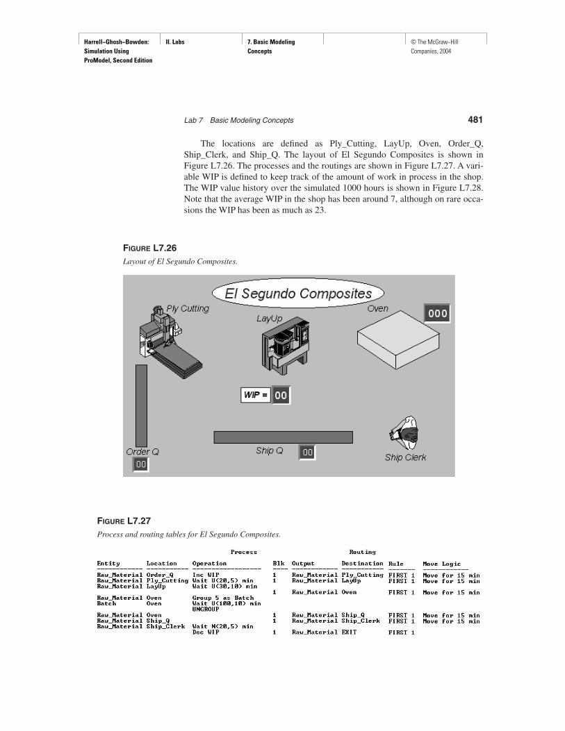
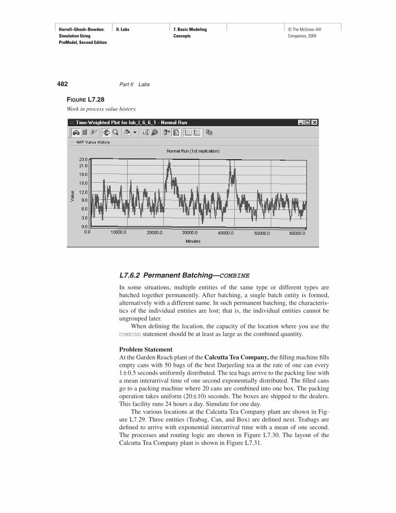
The locations are defined as Ply_Cutting, LayUp, Oven, Order_Q,Ship_Clerk, and Ship_Q. The layout of El Segundo Composites is shown inFigure L7.26. The processes and the routings are shown in Figure L7.27. A vari-able WIP is defined to keep track of the amount of work in process in the shop.The WIP value history over the simulated 1000 hours is shown in Figure L7.28.Note that the average WIP in the shop has been around 7, although on rare occa-sions the WIP has been as much as 23.

FIGURE L7.26Layout of El Segundo Composites.

FIGURE L7.27Process and routing tables for El Segundo Composites.




482 Part II Labs

L7.6.2 Permanent Batching—COMBINE

In some situations, multiple entities of the same type or different types arebatched together permanently. After batching, a single batch entity is formed,alternatively with a different name. In such permanent batching, the characteris-tics of the individual entities are lost; that is, the individual entities cannot beungrouped later.

When defining the location, the capacity of the location where you use theCOMBINE statement should be at least as large as the combined quantity.

Problem StatementAt the Garden Reach plant of the Calcutta Tea Company, the filling machine fillsempty cans with 50 bags of the best Darjeeling tea at the rate of one can every1±0.5 seconds uniformly distributed. The tea bags arrive to the packing line witha mean interarrival time of one second exponentially distributed. The filled cansgo to a packing machine where 20 cans are combined into one box. The packingoperation takes uniform (20±10) seconds. The boxes are shipped to the dealers.This facility runs 24 hours a day. Simulate for one day.

The various locations at the Calcutta Tea Company plant are shown in Fig-ure L7.29. Three entities (Teabag, Can, and Box) are defined next. Teabags aredefined to arrive with exponential interarrival time with a mean of one second.The processes and routing logic are shown in Figure L7.30. The layout of theCalcutta Tea Company plant is shown in Figure L7.31.

FIGURE L7.28Work in process value history.





FIGURE L7.29Locations at the Calcutta Tea Company.

FIGURE L7.30Process and routing tables at the Calcutta Tea Company.

FIGURE L7.31Layout of the CalcuttaTea Company.




484 Part II Labs

L7.7 Attaching One or More Entities to Another EntityL7.7.1 Permanent Attachment—JOIN

Sometimes one or more entities are attached permanently to another entity, as inan assembly operation. The assembly process is a permanent bonding: the assem-bled entities lose their separate identities and properties. The individual entitiesthat are attached cannot be separated again.

The join process is used to permanently assemble two or more individual en-tities together. For every JOIN statement, there must be a corresponding If JoinRequest rule. Joining is a two-step process:

1. Use the JOIN statement at the designated assembly location.

2. Use the join routing rule for all joining entities.

One of the joining entities, designated as the “base” entity, issues the JOIN state-ment. All other joining entities must travel to the assembly location on an If JoinRequest routing rule.

Problem StatementAt Shipping Boxes Unlimited computer monitors arrive at Monitor_Q at the rateof one every 15 minutes (exponential) and are moved to the packing table. Boxesarrive at Box_Q, at an average rate of one every 15 minutes (exponential) and arealso moved to the packing table. At the packing table, monitors are packed intoboxes. The packing operation takes normal (5,1) minutes. Packed boxes are sentto the inspector (Inspect_Q). The inspector checks the contents of the box andtallies with the packing slip. Inspection takes normal (4,2) minutes. After inspec-tion, the boxes are loaded into trucks at the shipping dock (Shipping_Q). Theloading takes uniform (5,1) minutes. Simulate for 100 hours. Track the number ofmonitors shipped and the WIP of monitors in the system.

The locations at Shipping Boxes Unlimited are defined as Monitor_Q,Box_Q, Shipping_Q, Inspect_Q, Shipping_Dock, Packing_Table, and Inspector.All the queue locations are defined with a capacity of infinity. Three entities(Monitor, Empty Box, and Full_Box) are defined next. The arrivals of monitorsand empty boxes are shown in Figure L7.32. The processes and routingsare shown in Figure L7.33. A snapshot of the simulation model is captured in

FIGURE L7.32Arrival of monitors and empty boxes at Shipping Boxes Unlimited.





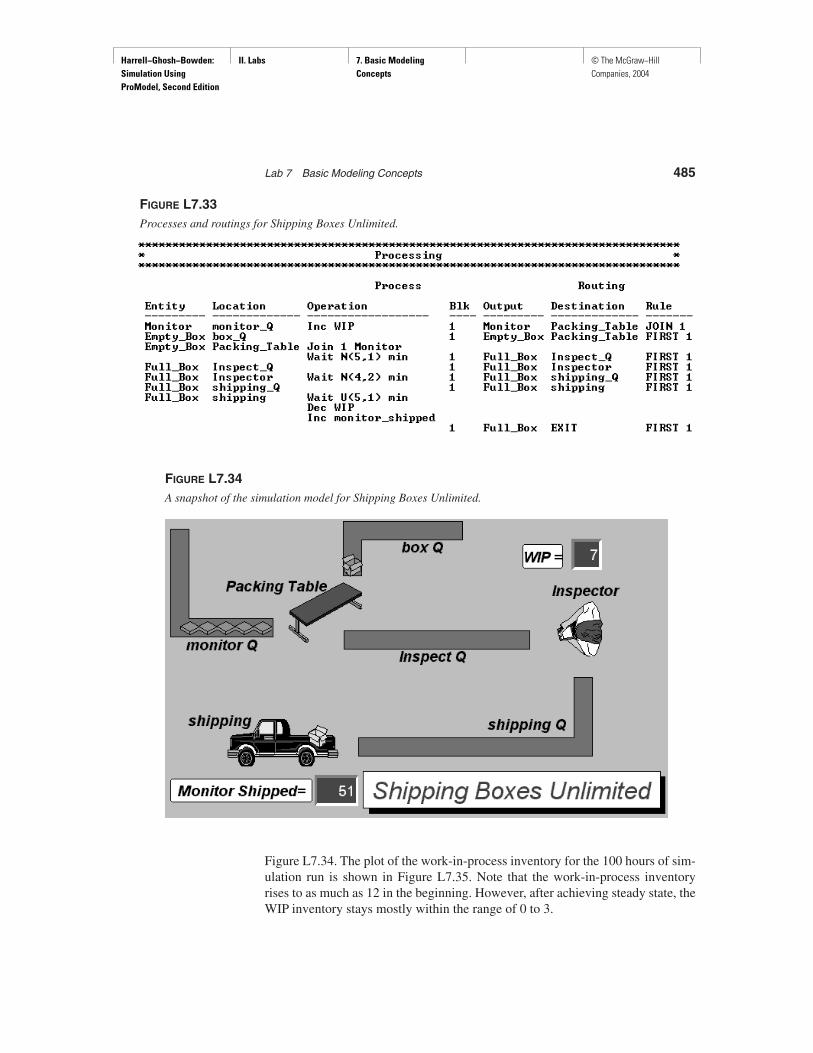
FIGURE L7.33Processes and routings for Shipping Boxes Unlimited.

FIGURE L7.34A snapshot of the simulation model for Shipping Boxes Unlimited.

Figure L7.34. The plot of the work-in-process inventory for the 100 hours of sim-ulation run is shown in Figure L7.35. Note that the work-in-process inventoryrises to as much as 12 in the beginning. However, after achieving steady state, theWIP inventory stays mostly within the range of 0 to 3.




486 Part II Labs

L7.7.2 Temporary Attachment—LOAD/UNLOAD

Sometimes one or more entities are attached to another entity temporarily,processed or moved together, and detached later in the system. In ProModel, weuse the LOAD and UNLOAD statements to achieve that goal. The properties of the in-dividual attached entities are preserved. This of course requires more memoryspace and hence should be used only when necessary.

Problem StatementFor the Shipping Boxes Unlimited problem in Section L7.7.1, assume the in-spector places (loads) a packed box on an empty pallet. The loading takes any-where from two to four minutes, uniformly distributed. The loaded pallet is sentto the shipping dock and waits in the shipping queue. At the shipping dock, thepacked boxes are unloaded from the pallet. The unloading time is also uniformlydistributed; U(3,1) min. The boxes go onto a waiting truck. The empty pallet is re-turned, via the pallet queue, to the inspector. One pallet is used and recirculated inthe system. Simulate for 100 hours. Track the number of monitors shipped and theWIP of monitors.

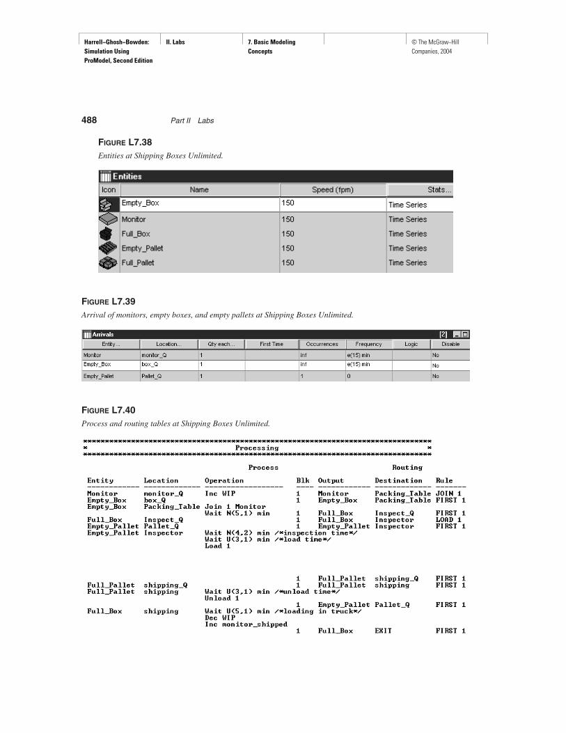
The locations defined in this model are Monitor_Q, Box_Q, Inspect_Q, Ship-ping_Q, Pallet_Q, Packing_Table, Inspector, and Shipping_Dock (Figure L7.36).All queue locations have infinite capacity. The layout of Shipping Boxes Unlim-ited is shown in Figure L7.37. Five entities are defined: Monitor, Box,Empty_Box, Empty_Pallet, and Full_Pallet as shown in Figure L7.38. The

FIGURE L7.35Time-weighted plot of the WIP inventory at Shipping Boxes Unlimited.





FIGURE L7.37Boxes loaded onpallets at ShippingBoxes Unlimited.

FIGURE L7.36The locations at Shipping Boxes Unlimited.

arrivals of monitors, empty boxes, and empty pallets are shown in Figure L7.39.The processes and routings are shown in Figure L7.40. Note that comments canbe inserted in a line of code as follows (Figure L7.40):

/* inspection time */

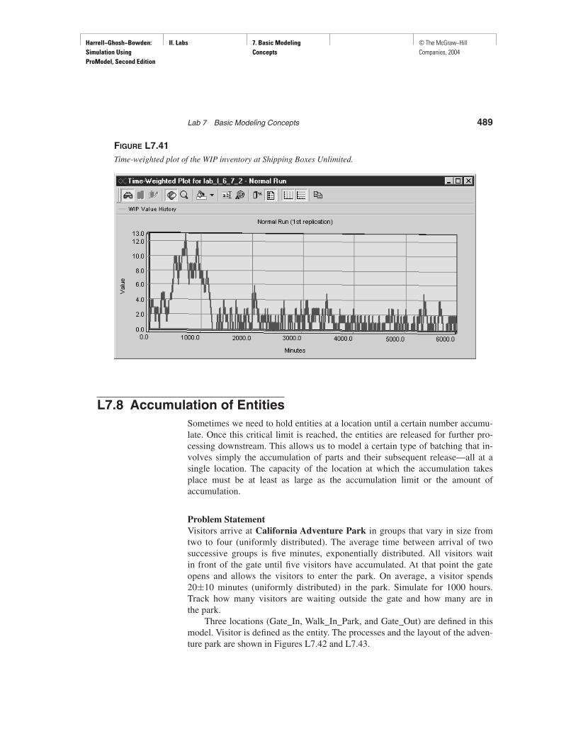
The plot of the work-in-process inventory for the 100 hours of simulation runis presented in Figure L7.41. Note that after the initial transient period (∼=1200minutes), the work-in-process inventory drops and stays mostly in a range of 0–2.




488 Part II Labs

FIGURE L7.39Arrival of monitors, empty boxes, and empty pallets at Shipping Boxes Unlimited.

FIGURE L7.40Process and routing tables at Shipping Boxes Unlimited.

FIGURE L7.38Entities at Shipping Boxes Unlimited.





L7.8 Accumulation of EntitiesSometimes we need to hold entities at a location until a certain number accumu-late. Once this critical limit is reached, the entities are released for further pro-cessing downstream. This allows us to model a certain type of batching that in-volves simply the accumulation of parts and their subsequent release—all at asingle location. The capacity of the location at which the accumulation takesplace must be at least as large as the accumulation limit or the amount ofaccumulation.

Problem StatementVisitors arrive at California Adventure Park in groups that vary in size fromtwo to four (uniformly distributed). The average time between arrival of twosuccessive groups is five minutes, exponentially distributed. All visitors waitin front of the gate until five visitors have accumulated. At that point the gateopens and allows the visitors to enter the park. On average, a visitor spends20±10 minutes (uniformly distributed) in the park. Simulate for 1000 hours.Track how many visitors are waiting outside the gate and how many are inthe park.

Three locations (Gate_In, Walk_In_Park, and Gate_Out) are defined in thismodel. Visitor is defined as the entity. The processes and the layout of the adven-ture park are shown in Figures L7.42 and L7.43.

FIGURE L7.41Time-weighted plot of the WIP inventory at Shipping Boxes Unlimited.




490 Part II Labs

L7.9 Splitting of One Entity into Multiple EntitiesWhen a single incoming entity is divided into multiple entities at a location andprocessed individually, we can use the SPLIT construct. The SPLIT commandsplits the entity into a specified number of entities, and optionally assigns them anew name. The resulting entities will have the same attribute values as the origi-nal entity. Use SPLIT to divide a piece of raw material into components, such as asilicon wafer into silicon chips or six-pack of cola into individual cans.

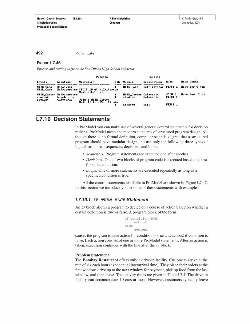
Problem StatementThe cafeteria at San Dimas High School receives 10 cases of milk from a vendoreach day before the lunch recess. On receipt, the cases are split open and individual

FIGURE L7.43Layout of California Adventure Park.

FIGURE L7.42Process and routing tables for California Adventure Park.





cartons (10 per case) are stored in the refrigerator for distribution to students dur-ing lunchtime. The distribution of milk cartons takes triangular(.1,.15,.2) minuteper student. The time to split open the cases takes a minimum of 5 minutes and amaximum of 7 minutes (uniform distribution) per case. Moving the cases from re-ceiving to the refrigerator area takes five minutes per case, and moving the cartonsfrom the refrigerator to the distribution area takes 0.2 minute per carton. Studentswait in the lunch line to pick up one milk carton each. There are only 100 studentsat this high school. Students show up for lunch with a mean interarrival time of1 minute (exponential). On average, how long does a carton stay in the cafeteriabefore being distributed and consumed? What are the maximum and the minimumtimes of stay? Simulate for 10 days.

The layout of the San Dimas High School cafeteria is shown in Figure L7.44.Three entities—Milk_Case, Milk_Carton, and Student—are defined. Ten milkcases arrive with a frequency of 480 minutes. One hundred students show up forlunch each day. The arrival of students and milk cases is shown in Figure L7.45.The processing and routing logic is shown in Figure L7.46.

FIGURE L7.44Layout of the San Dimas High School cafeteria.

FIGURE L7.45Arrival of milk and students at the San Dimas High School cafeteria.




492 Part II Labs

L7.10 Decision StatementsIn ProModel you can make use of several general control statements for decisionmaking. ProModel meets the modern standards of structured program design. Al-though there is no formal definition, computer scientists agree that a structuredprogram should have modular design and use only the following three types oflogical structures: sequences, decisions, and loops.

• Sequences: Program statements are executed one after another.

• Decisions: One of two blocks of program code is executed based on a testfor some condition.

• Loops: One or more statements are executed repeatedly as long as aspecified condition is true.

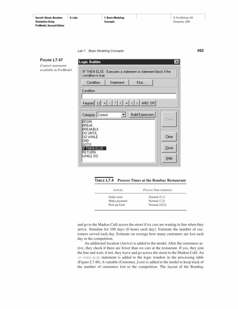
All the control statements available in ProModel are shown in Figure L7.47.In this section we introduce you to some of these statements with examples.

L7.10.1 IF-THEN-ELSE Statement

An IF block allows a program to decide on a course of action based on whether acertain condition is true or false. A program block of the form

IF condition THENaction1

ELSEaction2

causes the program to take action1 if condition is true and action2 if condition isfalse. Each action consists of one or more ProModel statements. After an action istaken, execution continues with the line after the IF block.

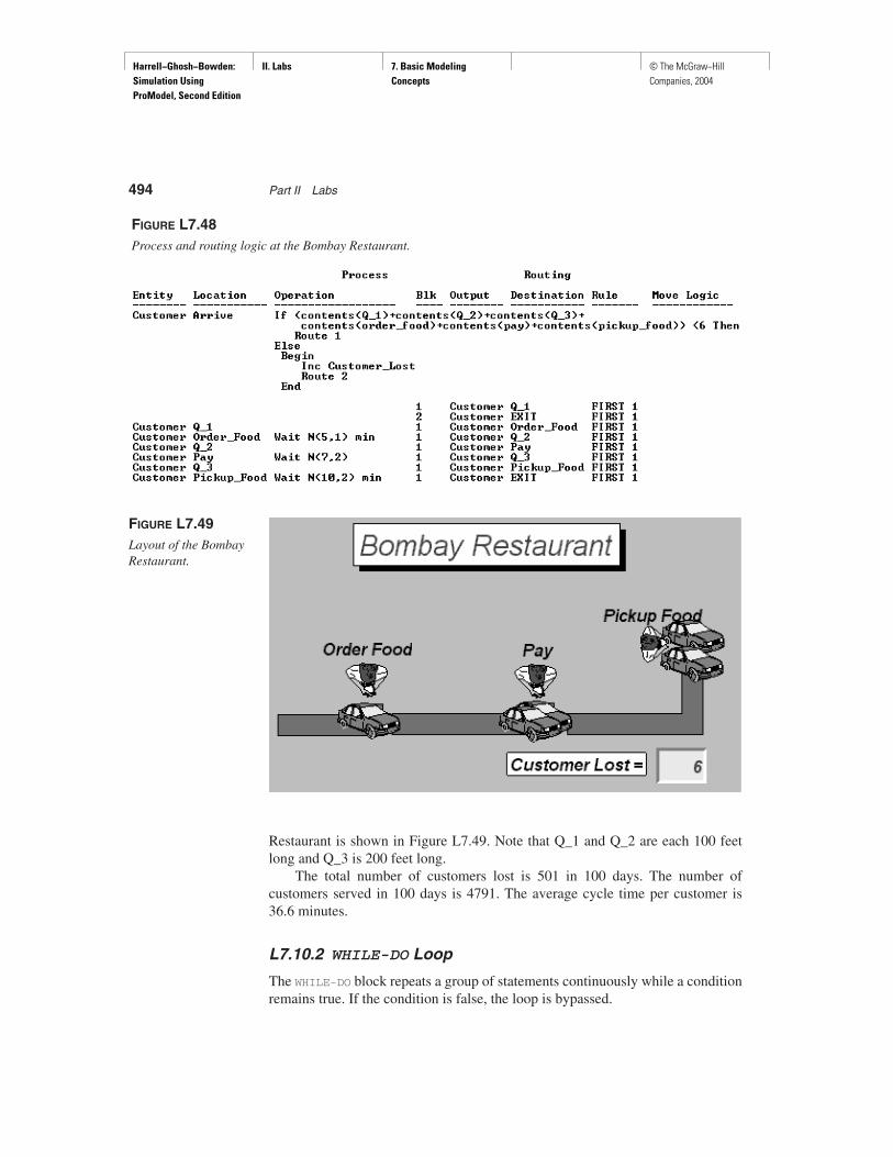
Problem Statement The Bombay Restaurant offers only a drive-in facility. Customers arrive at therate of six each hour (exponential interarrival time). They place their orders at thefirst window, drive up to the next window for payment, pick up food from the lastwindow, and then leave. The activity times are given in Table L7.4. The drive-infacility can accommodate 10 cars at most. However, customers typically leave

FIGURE L7.46Process and routing logic at the San Dimas High School cafeteria.





and go to the Madras Café across the street if six cars are waiting in line when theyarrive. Simulate for 100 days (8 hours each day). Estimate the number of cus-tomers served each day. Estimate on average how many customers are lost eachday to the competition.

An additional location (Arrive) is added to the model. After the customers ar-rive, they check if there are fewer than six cars at the restaurant. If yes, they jointhe line and wait; if not, they leave and go across the street to the Madras Café. AnIF-THEN-ELSE statement is added to the logic window in the processing table(Figure L7.48). A variable (Customer_Lost) is added to the model to keep track ofthe number of customers lost to the competition. The layout of the Bombay

FIGURE L7.47Control statementsavailable in ProModel.

TABLE L7.4 Process Times at the Bombay Restaurant

Activity Process Time (minutes)

Order food Normal (5,1)Make payment Normal (7,2)Pick up food Normal (10,2)




Restaurant is shown in Figure L7.49. Note that Q_1 and Q_2 are each 100 feetlong and Q_3 is 200 feet long.

The total number of customers lost is 501 in 100 days. The number ofcustomers served in 100 days is 4791. The average cycle time per customer is36.6 minutes.

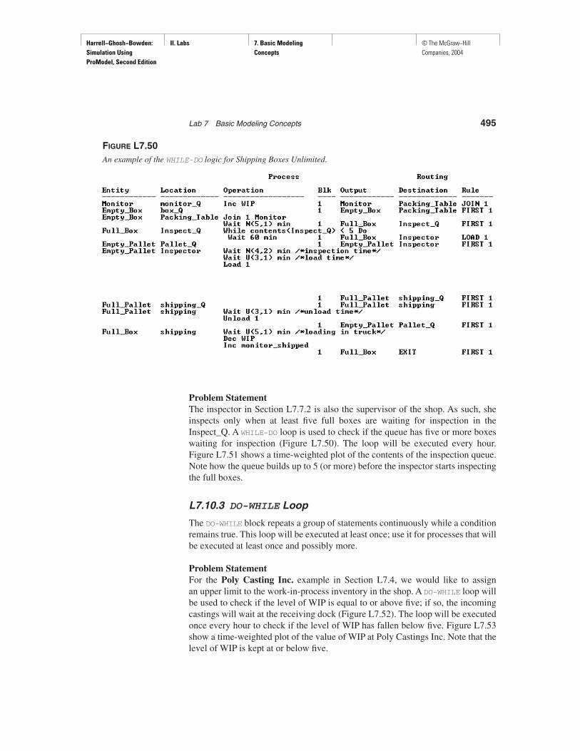
L7.10.2 WHILE-DO Loop

The WHILE-DO block repeats a group of statements continuously while a conditionremains true. If the condition is false, the loop is bypassed.

494 Part II Labs

FIGURE L7.49Layout of the BombayRestaurant.

FIGURE L7.48Process and routing logic at the Bombay Restaurant.





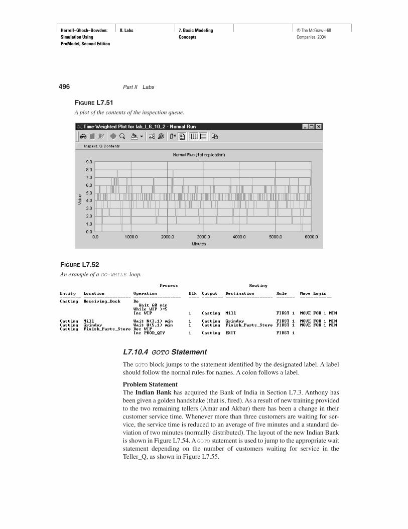
Problem StatementThe inspector in Section L7.7.2 is also the supervisor of the shop. As such, sheinspects only when at least five full boxes are waiting for inspection in theInspect_Q. A WHILE-DO loop is used to check if the queue has five or more boxeswaiting for inspection (Figure L7.50). The loop will be executed every hour.Figure L7.51 shows a time-weighted plot of the contents of the inspection queue.Note how the queue builds up to 5 (or more) before the inspector starts inspectingthe full boxes.

L7.10.3 DO-WHILE Loop

The DO-WHILE block repeats a group of statements continuously while a conditionremains true. This loop will be executed at least once; use it for processes that willbe executed at least once and possibly more.

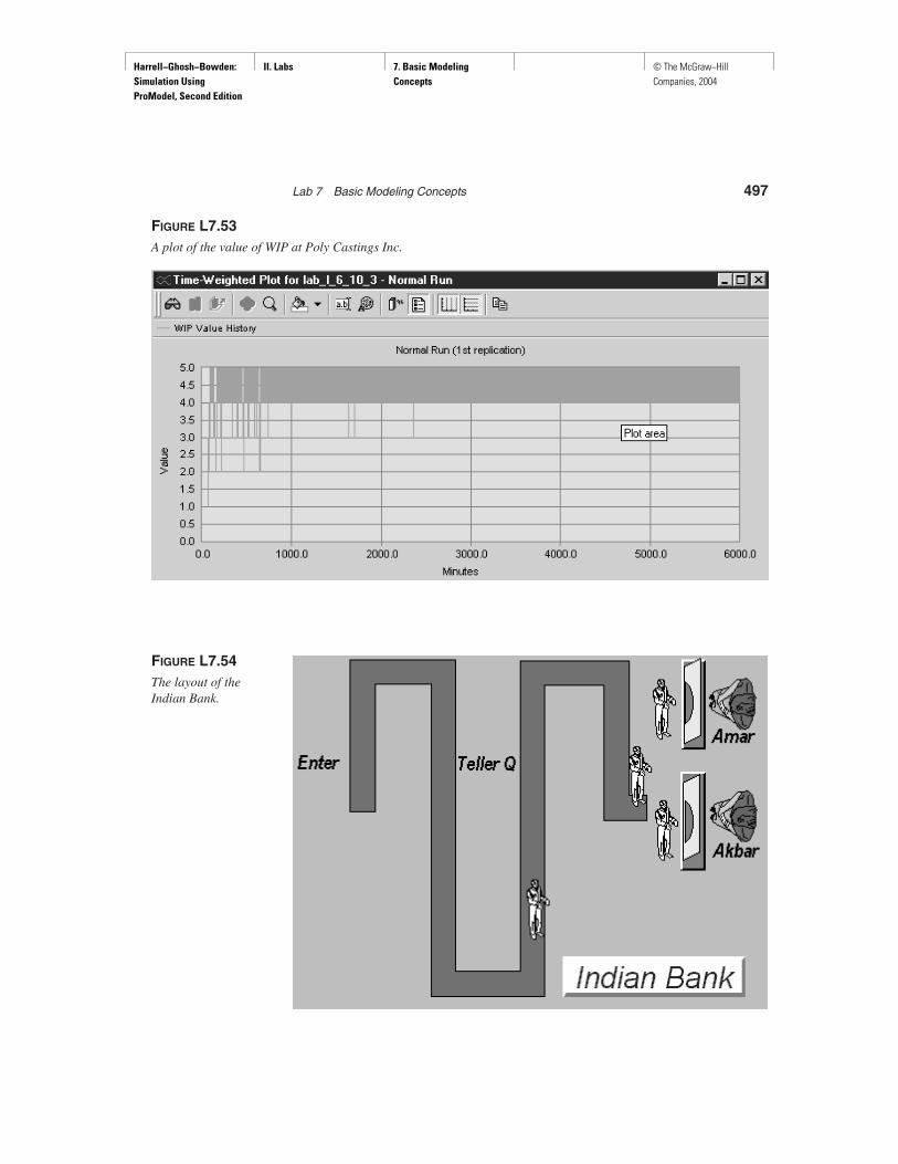
Problem StatementFor the Poly Casting Inc. example in Section L7.4, we would like to assignan upper limit to the work-in-process inventory in the shop. A DO-WHILE loop willbe used to check if the level of WIP is equal to or above five; if so, the incomingcastings will wait at the receiving dock (Figure L7.52). The loop will be executedonce every hour to check if the level of WIP has fallen below five. Figure L7.53show a time-weighted plot of the value of WIP at Poly Castings Inc. Note that thelevel of WIP is kept at or below five.

FIGURE L7.50An example of the WHILE-DO logic for Shipping Boxes Unlimited.




496 Part II Labs

FIGURE L7.51A plot of the contents of the inspection queue.

L7.10.4 GOTO Statement

The GOTO block jumps to the statement identified by the designated label. A labelshould follow the normal rules for names. A colon follows a label.

Problem StatementThe Indian Bank has acquired the Bank of India in Section L7.3. Anthony hasbeen given a golden handshake (that is, fired). As a result of new training providedto the two remaining tellers (Amar and Akbar) there has been a change in theircustomer service time. Whenever more than three customers are waiting for ser-vice, the service time is reduced to an average of five minutes and a standard de-viation of two minutes (normally distributed). The layout of the new Indian Bankis shown in Figure L7.54. A GOTO statement is used to jump to the appropriate waitstatement depending on the number of customers waiting for service in theTeller_Q, as shown in Figure L7.55.

FIGURE L7.52An example of a DO-WHILE loop.





FIGURE L7.53A plot of the value of WIP at Poly Castings Inc.

FIGURE L7.54The layout of theIndian Bank.




498 Part II Labs

L7.11 Periodic System ShutdownSome service systems periodically stop admitting new customers for a given du-ration to catch up on the backlog of work and reduce the congestion. Some auto-mobile service centers, medical clinics, restaurants, amusement parks, and banksuse this strategy. The modulus mathematical operator in ProModel is useful forsimulating such periodic shutdowns.

Problem StatementThe Bank of India in Section L7.3 opens for business each day for 8 hours (480minutes). Assume that the customers arrive to the bank according to an exponen-tial distribution (mean of 4 minutes). All the tellers service the customers accord-ing to a uniform distribution (mean of 10 minutes and half-width of 6 minutes).Customers are routed to the three tellers in turn (selected in rotation).

Each day after 300 minutes (5 hours) of operation, the front door of the bankis locked, and any new customers arriving at the bank are turned away. Customersalready inside the bank continue to get served. The bank reopens the front door90 minutes (1.5 hours) later to new customers. Simulate the system for 480 min-utes (8 hours). Make a time-series plot of the Teller_Q to show the effect of lock-ing the front door on the bank.

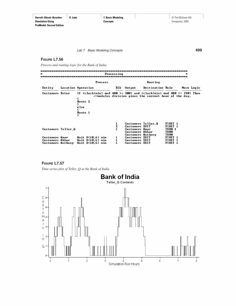
The logic for locking the front door is shown in Figure L7.56. The simulationclock time clock(min) is a cumulative counter of hours elapsed since the start ofthe simulation run. The current time of any given day can be determined by mod-ulus dividing the current simulation time, clock(min), by 480 minutes. If the re-mainder of clock(min) divided by 480 minutes is between 300 minutes (5 hours)and 390 minutes (6.5 hours), the arriving customers are turned away (disposed).Otherwise, they are allowed into the bank. An IF-THEN-ELSE logic block as de-scribed in Section L7.10.1 is used here.

A time-series plot of the contents of the Teller_Q is shown in Figure L7.57.This plot clearly shows how the Teller_Q (and the whole bank) builds up during

FIGURE L7.55An example of a GOTO statement.





FIGURE L7.56Process and routing logic for the Bank of India.

FIGURE L7.57Time-series plot of Teller_Q at the Bank of India.




500 Part II Labs

FIGURE L7.58Histogram of Teller_Q contents at the Bank of India.

the day; then, after the front door is locked at the fifth hour (300 minutes) into thesimulated day, customers remaining in the queue are processed and the queuelength decreases (down to zero in this particular simulation run). The queue lengthpicks back up when the bank reopens the front door at simulation time 6.5 hours(390 minutes).

The histogram of the same queue (Figure L7.58) shows that approximately49% of the time the queue was empty. About 70% of the time there are 3 or fewercustomers waiting in line. What is the average time a customer spends in thebank? Would you recommend that the bank not close the door after 5 hours of op-eration (customers never liked this practice anyway)? Will the average customerstay longer in the bank?

L7.12 Exercises1. Visitors arrive at Kid’s World entertainment park according to an

exponential interarrival time distribution with mean 2.5 minutes. Thetravel time from the entrance to the ticket window is normallydistributed with a mean of three minutes and a standard deviation of0.5 minute. At the ticket window, visitors wait in a single line until one





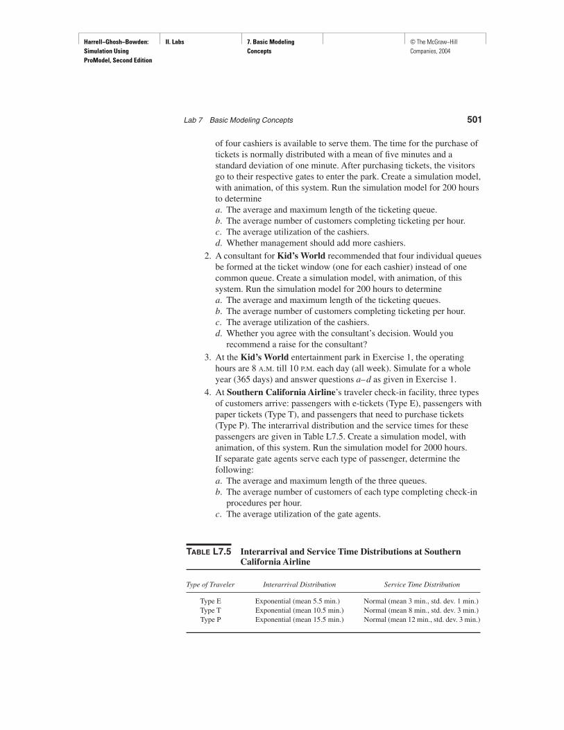
of four cashiers is available to serve them. The time for the purchase oftickets is normally distributed with a mean of five minutes and astandard deviation of one minute. After purchasing tickets, the visitorsgo to their respective gates to enter the park. Create a simulation model,with animation, of this system. Run the simulation model for 200 hoursto determinea. The average and maximum length of the ticketing queue.b. The average number of customers completing ticketing per hour.c. The average utilization of the cashiers.d. Whether management should add more cashiers.

2. A consultant for Kid’s World recommended that four individual queuesbe formed at the ticket window (one for each cashier) instead of onecommon queue. Create a simulation model, with animation, of thissystem. Run the simulation model for 200 hours to determinea. The average and maximum length of the ticketing queues.b. The average number of customers completing ticketing per hour.c. The average utilization of the cashiers.d. Whether you agree with the consultant’s decision. Would you

recommend a raise for the consultant?

3. At the Kid’s World entertainment park in Exercise 1, the operatinghours are 8 A.M. till 10 P.M. each day (all week). Simulate for a wholeyear (365 days) and answer questions a–d as given in Exercise 1.

4. At Southern California Airline’s traveler check-in facility, three typesof customers arrive: passengers with e-tickets (Type E), passengers withpaper tickets (Type T), and passengers that need to purchase tickets(Type P). The interarrival distribution and the service times for thesepassengers are given in Table L7.5. Create a simulation model, withanimation, of this system. Run the simulation model for 2000 hours.If separate gate agents serve each type of passenger, determine thefollowing:a. The average and maximum length of the three queues.b. The average number of customers of each type completing check-in

procedures per hour.c. The average utilization of the gate agents.

TABLE L7.5 Interarrival and Service Time Distributions at SouthernCalifornia Airline

Type of Traveler Interarrival Distribution Service Time Distribution

Type E Exponential (mean 5.5 min.) Normal (mean 3 min., std. dev. 1 min.)Type T Exponential (mean 10.5 min.) Normal (mean 8 min., std. dev. 3 min.)Type P Exponential (mean 15.5 min.) Normal (mean 12 min., std. dev. 3 min.)




502 Part II Labs

d. The percentage of time the number of customers (of each type ofcustomer) waiting in line is ≤ 2.

e. Would you recommend one single line for check-in for all three typesof travelers? Discuss the pros and cons of such a change.

5. Raja & Rani, a fancy restaurant in Santa Clara, holds a maximum of 15diners. Customers arrive according to an exponential distribution with amean of 5 minutes. Customers stay in the restaurant according to atriangular distribution with a minimum of 45 minutes, a maximum of 60minutes, and a mode of 75 minutes. Create a simulation model, withanimation, of this system. The restaurant operating hours are 3 P.M. till12 P.M. Run the simulation model for 50 replications of 9 hours each.a. Beginning empty, how long (average and standard deviation) does it

take for the restaurant to fill?b. What is the total number of diners (average and standard deviation)

entering the restaurant before it fills?c. What is the total number of guests (average and standard deviation)

served per night?d. What is the average utilization of the restaurant?

6. Woodland Nursing Home has six departments—initial exam, X ray,operating room, cast-fitting room, recovery room, and checkout room.The probabilities that a patient will go from one department to anotherare given in Table L7.6. The time patients spend in each department isgiven in Table L7.7. Patients arrive at the average rate of 5 per hour(exponential interarrival time). The nursing home remains open 24/7.

TABLE L7.6 Probabilities of Patient Flow

From To Probability

Initial exam X ray .35Operating room .20Recovery room .15Checkout room .30

X ray Operating room .15Cast-fitting room .25Recovery room .40Checkout room .20

Operating room Cast-fitting room .30Recovery room .65Checkout room .05

Cast-fitting room Recovery room .55X ray .10Checkout room .35

Recovery room Operating room .10X ray .20Checkout room .70





TABLE L7.7 Patient Processing Time

Department Patient Time in Department

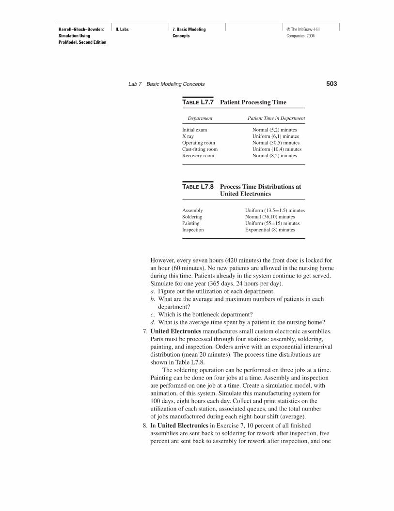
Initial exam Normal (5,2) minutesX ray Uniform (6,1) minutesOperating room Normal (30,5) minutesCast-fitting room Uniform (10,4) minutesRecovery room Normal (8,2) minutes

TABLE L7.8 Process Time Distributions atUnited Electronics

Assembly Uniform (13.5±1.5) minutesSoldering Normal (36,10) minutesPainting Uniform (55±15) minutesInspection Exponential (8) minutes

However, every seven hours (420 minutes) the front door is locked foran hour (60 minutes). No new patients are allowed in the nursing homeduring this time. Patients already in the system continue to get served.Simulate for one year (365 days, 24 hours per day).a. Figure out the utilization of each department. b. What are the average and maximum numbers of patients in each

department?c. Which is the bottleneck department?d. What is the average time spent by a patient in the nursing home?

7. United Electronics manufactures small custom electronic assemblies.Parts must be processed through four stations: assembly, soldering,painting, and inspection. Orders arrive with an exponential interarrivaldistribution (mean 20 minutes). The process time distributions areshown in Table L7.8.

The soldering operation can be performed on three jobs at a time.Painting can be done on four jobs at a time. Assembly and inspectionare performed on one job at a time. Create a simulation model, withanimation, of this system. Simulate this manufacturing system for100 days, eight hours each day. Collect and print statistics on theutilization of each station, associated queues, and the total numberof jobs manufactured during each eight-hour shift (average).

8. In United Electronics in Exercise 7, 10 percent of all finishedassemblies are sent back to soldering for rework after inspection, fivepercent are sent back to assembly for rework after inspection, and one




504 Part II Labs

percent of all assemblies fail to pass and are scrapped. Create asimulation model, with animation, of this system. Simulate thismanufacturing system for 100 days, eight hours each day. Collect andprint statistics on the utilization of each station, associated queues, totalnumber of jobs assembled, number of assemblies sent for rework toassembly and soldering, and the number of assemblies scrapped duringeach eight-hour shift (average).

9. Small toys are assembled in four stages (Centers 1, 2, and 3 andInspection) at Bengal Toy Company. After each assembly step, theappliance is inspected or tested; if a defect is found, it must be correctedand then checked again. The assemblies arrive at a constant rate of oneassembly every two minutes. The times to assemble, test, and correctdefects are normally distributed. The means and standard deviations ofthe times to assemble, inspect, and correct defects, as well as thelikelihood of an assembly error, are shown in Table L7.9. If an assemblyis found defective, the defect is corrected and it is inspected again. Aftera defect is corrected, the likelihood of another defect being found is thesame as during the first inspection. We assume in this model that anassembly defect is eventually corrected and then it is passed on to thenext station. Simulate for one year (2000 hours) and determine thenumber of good toys shipped in a year.

10. Salt Lake City Electronics manufactures small custom communicationequipment. Two different job types are to be processed within thefollowing manufacturing cell. The necessary data are given inTable L7.10. Simulate the system to determine the average number ofjobs waiting for different operations, number of jobs of each typefinished each day, average cycle time for each type of job, and theaverage cycle time for all jobs.

11. Six dump trucks at the DumpOnMe facility in Riverside are used tohaul coal from the entrance of a small mine to the railroad. FigureL7.59 provides a schematic of the dump truck operation. Each truck isloaded by one of two loaders. After loading, a truck immediately moves

TABLE L7.9 Process Times and Probability of Defects at BengalToy Company

Assembly Time Inspect Time Correct Time

Standard Standard StandardCenter Mean Deviation Mean Deviation P(error) Mean Deviation

1 .7 .2 .2 .05 .1 .2 .052 .75 .25 .2 .05 .05 .15 .043 .8 .15 .15 .03 .03 .1 .02





to the scale to be weighed as soon as possible. Both the loaders and thescale have a first-come, first-served waiting line (or queue) for trucks.Travel time from a loader to the scale is considered negligible. Afterbeing weighed, a truck begins travel time (during which time the truckunloads), and then afterward returns to the loader queue. Thedistributions of loading time, weighing time, and travel time are shownin Table L7.11.a. Create a simulation model, with animation, of this system. Simulate

for 200 days, eight hours each day.b. Collect statistics to estimate the loader and scale utilization

(percentage of time busy).c. About how many trucks are loaded each day on average?

TABLE L7.10 Data Collected at Salt Lake City Electronics

Number TimeNumber of Jobs between

Job of per Assembly Soldering Painting Inspection BatchType Batches Batch Time Time Time Time Arrivals

1 15 5 Tria (5,7,10) Normal (36,10) Uniform (55±15) Exponential (8) Exp (14)2 25 3 Tria (7,10,15) Uniform (35±5) Exponential (5) Exp (10)

Note: All times are given in minutes.

TABLE L7.11 Various Time Measurement Dataat the DumpOnMe Facility

Loading time Uniform (7.5±2.5) minutesWeighing time Uniform (3.5±1.5) minutesTravel time Triangular (10,12,15) minutes

FIGURE L7.59Schematic of dumptruck operation forDumpOnMe.

Loader queue Weighing queueWeighing

scale

Loader 1

Loader 2

Truck traveland unload




12. At the Pilot Pen Company, a molding machine produces pen barrels oftwo different colors—red and blue—in the ratio of 3:2. The moldingtime is triangular (3,4,6) minutes per barrel. The barrels go to a fillingmachine, where ink of appropriate color is filled at the rate of 20 pensper hour (exponentially distributed). Another molding machine makescaps of the same two colors in the ratio of 3:2. The molding time istriangular (3,4,6) minutes per cap. At the next station, caps and filledbarrels of matching colors are joined together. The joining time isexponentially distributed with a mean of 1 min. Simulate for 2000 hours.Find the average number of pens produced per hour. Collect statistics onthe utilization of the molding machines and the joining equipment.

13. Customers arrive at the NoWaitBurger hamburger stand with aninterarrival time that is exponentially distributed with a mean of oneminute. Out of 10 customers, 5 buy a hamburger and a drink, 3 buy ahamburger, and 2 buy just a drink. One server handles the hamburgerwhile another handles the drink. A person buying both items needs towait in line for both servers. The time it takes to serve a customer isN(70,10) seconds for each item. Simulate for 100 hours. Collectstatistics on the number of customers served per hour, size of thequeues, and utilization of the servers. What changes would you suggestto make the system more efficient?

14. Workers who work at the Detroit ToolNDie plant must check out toolsfrom a tool crib. Workers arrive according to an exponential distributionwith a mean time between arrivals of five minutes. At present, three toolcrib clerks staff the tool crib. The time to serve a worker is normallydistributed with a mean of 10 minutes and a standard deviation of2 minutes. Compare the following servicing methods. Simulate for2000 hours and collect data.a. Workers form a single queue, choosing the next available tool crib

clerk.b. Workers enter the shortest queue (each clerk has his or her own

queue).c. Workers choose one of three queues at random.

15. At the ShopNSave, a small family-owned grocery store, there are onlyfour aisles: aisle 1—fruits/vegetables, aisle 2—packaged goods (cerealsand the like), aisle 3—dairy products, and aisle 4—meat/fish. The timebetween two successive customer arrivals is exponentially distributedwith a mean of 5 minutes. After arriving to the store, each customergrabs a shopping cart. Twenty percent of all customers go to aisle 1,30 percent go to aisle 2, 50 percent go to aisle 3, and 70 percent go toaisle 4. The number of items selected for purchase in each aisle isuniformly distributed between 2 and 8. The time spent to browse andpick up each item is normally distributed: N(5,2) minutes. There arethree identical checkout counters; each counter has its own checkout

506 Part II Labs





line. The customer chooses the shortest line. Once a customer joins aline, he or she is not allowed to leave or switch lines. The checkout timeis given by the following regression equation:

Checkout time = N(3,0.3) + (#of items) * N(0.5,0.15) minutes

The first term of the checkout time is for receiving cash or a check orcredit card from the customer, opening and closing the cash register,and handing over the receipt and cash to the customer. After checkingout, a customer leaves the cart at the front of the store and leaves. Builda simulation model for the grocery store. Use the model to simulate a14-hour day.a. The percentages of customers visiting each aisle do not add up

to 100 percent. Why?b. What is the average amount of time a customer spends at the

grocery store?c. How many customers check out per cashier per hour?d. What is the average amount of time a customer spends waiting in

the checkout line?e. What is the average utilization of the cashiers?f. Assuming there is no limit to the number of shopping carts,

determine the average and maximum number of carts in use at anytime.

g. On average how many customers are waiting in line to checkout?h. If the owner adopts a customer service policy that there will never

be any more than three customers in any checkout line, how manycashiers are needed?

Embellishments:I. The store manager is considering designating one of the checkout lines

as Express, for customers checking out with 10 or fewer items. Is that agood idea? Why or why not?

II. In reality, there are only 10 shopping carts at the ShopNSave store.If there are no carts available when customers arrive they leaveimmediately and go to the more expensive ShopNSpend store down thestreet. Modify the simulation model to reflect this change. How manycustomers are lost per hour? How many shopping carts should theyhave so that no more than 5 percent of customers are lost?

16. Planes arrive at the Netaji Subhash Chandra Bose InternationalAirport, Calcutta with interarrival times that are exponentiallydistributed with a mean time of 30 minutes. If there is no room at theairport when a plane arrives, the pilot flies around and comes back toland after a normally distributed time having a mean of 20 minutes anda standard deviation of 5 minutes. There are two runways and threegates at this small airport. The time from touchdown to arrival at a gateis normally distributed having a mean of five minutes and a standard




508 Part II Labs

deviation of one minute. A maximum of three planes can be unloadedand loaded at the airport at any time. The times to unload and load aplane are uniformly distributed between 20 and 30 minutes. Thepushoff, taxi, and takeoff times are normally distributed with a mean ofsix minutes and a standard deviation of one minute. The airport operates24/7. Build a simulation model and run it for one year.

a. How much will adding a new gate decrease the time that airplaneshave to circle before landing?

b. Will adding a new gate affect the turnaround time of airplanes at theairport? How much?

c. Is it better to add another runway instead of another gate? If so, why?

la b basic modeling concepts - brawijaya...

Documents