l3 apprentissage - lri.frsebag/slides/cachan_8_2013.pdf · strange clusterings... emporium of...
TRANSCRIPT
L3 Apprentissage
Michele Sebag − Benjamin MonmegeLRI − LSV
17 avril 2013
1

Overview
Introduction
Linear changes of representationPrincipal Component AnalysisRandom projectionsLatent Semantic Analysis
Non linear changes of representation
2
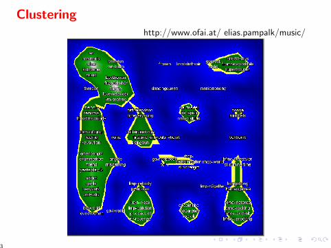
Clusteringhttp://www.ofai.at/ elias.pampalk/music/
3
Unsupervised learning
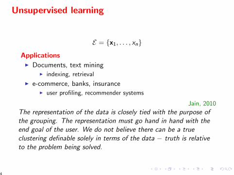
E = {x1, . . . , xn}
ApplicationsI Documents, text mining
I indexing, retrieval
I e-commerce, banks, insuranceI user profiling, recommender systems
Jain, 2010
The representation of the data is closely tied with the purpose ofthe grouping. The representation must go hand in hand with theend goal of the user. We do not believe there can be a trueclustering definable solely in terms of the data − truth is relativeto the problem being solved.
4
Unsupervised learning − WHAT
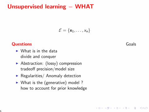
E = {x1, . . . , xn}
Questions Goals
I What is in the datadivide and conquer
I Abstraction: (lossy) compressiontradeoff precision/model size
I Regularities/ Anomaly detection
I What is the (generative) model ?how to account for prior knowledge
5

Unsupervised learning − HOW
Position of the problem Algorithmic issues
I Stationary data clustering; density estimation
I Online data Data streamingTradeoff precision / noise
I Non-stationary data:change detection / noise
Real-time ? Limited resources ?
Validation
I exploratory data analysis (subjective)
I density estimation (likelihood)
6

AbstractionArtifacts
I Represent a set of instances xi ∈ X by an element z ∈ XI Examples:
I Mean state of a systemI Sociological profile
Prototypes
I Find the most representatives instances among x1, . . . xnI How many prototypes ? (avoid overfitting)I Examples:
I FacesI Molecules
7
Generative models
GivenE = {xi ∈ X} P(x)
Find P(x).
Issues
I A distribution (sums to 1)
I Parametric (e.g. mixture of Gaussians) vs non- ?
I Which criterion ? optimize (log) likelihood of data.
8
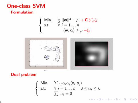
One-class SVMFormulation
Min. 12 ||w||
2 − ρ + C∑
i ξi
s.t. ∀ i = 1 . . . n〈w, xi 〉 ≥ ρ −ξi
Dual problemMin.
∑i ,j αiαj〈xi , xj〉
s.t. ∀ i = 1 . . . n 0 ≤ αi ≤ C∑i αi = 0
9
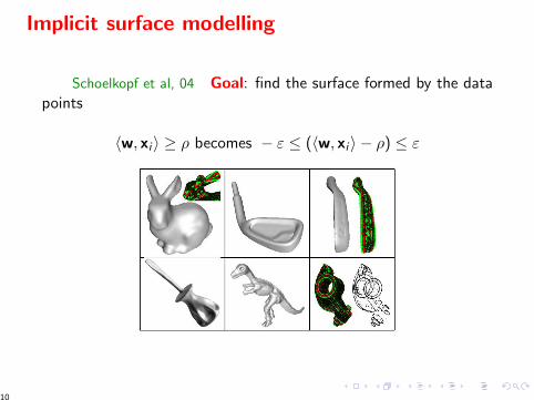
Implicit surface modelling
Schoelkopf et al, 04 Goal: find the surface formed by the datapoints
〈w, xi 〉 ≥ ρ becomes − ε ≤ (〈w, xi 〉 − ρ) ≤ ε
10
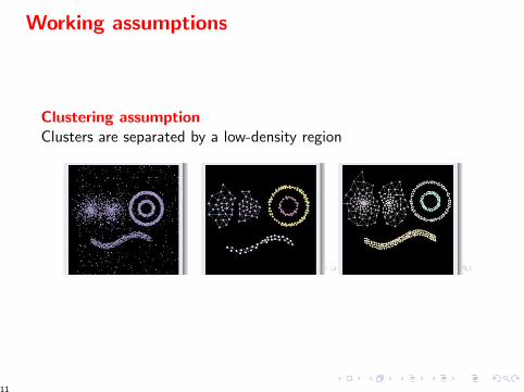
Working assumptions
Clustering assumptionClusters are separated by a low-density region
11

Strange clusterings...
http://en.wikipedia.org/wiki/Celestial Emporium of Benevolent Knowledge%27s Taxonomy
... a certain Chinese encyclopedia called the Heavenly Emporiumof Benevolent Knowledge.In its distant pages it is written that animals are divided into (a)those that belong to the emperor; (b) embalmed ones; (c) thosethat are trained; (d) suckling pigs; (e) mermaids; (f) fabulousones; (g) stray dogs; (h) those that are included in thisclassification; (i) those that tremble as if they were mad; (j)innumerable ones; (k) those drawn with a very fine camel’s-hairbrush; (l) etcetera; (m) those that have just broken the flowervase; (n) those that at a distance resemble flies. Borges, 1942
12

Overview
Introduction
Linear changes of representationPrincipal Component AnalysisRandom projectionsLatent Semantic Analysis
Non linear changes of representation
13
Dimensionality Reduction − Intuition
Degrees of freedom
I Image: 4096 pixels; but not independent
I Robotics: (# camera pixels + # infra-red) × time; but notindependent
GoalFind the (low-dimensional) structure of the data:
I Images
I Robotics
I Genes
14
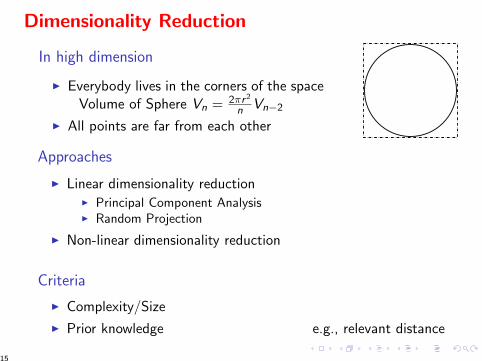
Dimensionality Reduction
In high dimension
I Everybody lives in the corners of the spaceVolume of Sphere Vn = 2πr2
n Vn−2
I All points are far from each other
Approaches
I Linear dimensionality reductionI Principal Component AnalysisI Random Projection
I Non-linear dimensionality reduction
Criteria
I Complexity/Size
I Prior knowledge e.g., relevant distance
15
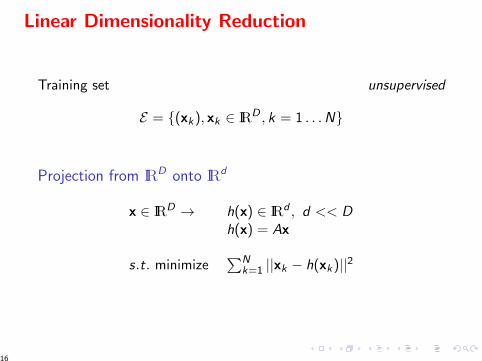
Linear Dimensionality Reduction
Training set unsupervised
E = {(xk), xk ∈ IRD , k = 1 . . .N}
Projection from IRD onto IRd
x ∈ IRD → h(x) ∈ IRd , d << Dh(x) = Ax
s.t. minimize∑N
k=1 ||xk − h(xk)||2
16

Overview
Introduction
Linear changes of representationPrincipal Component AnalysisRandom projectionsLatent Semantic Analysis
Non linear changes of representation
17
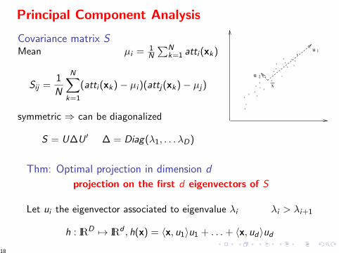
Principal Component Analysis
Covariance matrix SMean µi = 1
N
∑Nk=1 atti (xk)
Sij =1
N
N∑k=1
(atti (xk)− µi )(attj(xk)− µj)
symmetric ⇒ can be diagonalized
S = U∆U ′ ∆ = Diag(λ1, . . . λD)
xx
x
xx
xx
x
x
xx
x
xx
xx
x
u
u
x
1
2
x
x
x
x
x
x
x
Thm: Optimal projection in dimension d
projection on the first d eigenvectors of S
Let ui the eigenvector associated to eigenvalue λi λi > λi+1
h : IRD 7→ IRd , h(x) = 〈x, u1〉u1 + . . .+ 〈x, ud〉ud
18
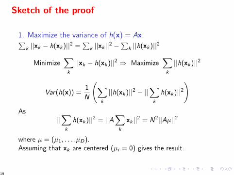
Sketch of the proof
1. Maximize the variance of h(x) = Ax∑k ||xk − h(xk)||2 =
∑k ||xk ||2 −
∑k ||h(xk)||2
Minimize∑k
||xk − h(xk)||2 ⇒ Maximize∑k
||h(xk)||2
Var(h(x)) =1
N
(∑k
||h(xk)||2 − ||∑k
h(xk)||2)
As||∑k
h(xk)||2 = ||A∑k
xk ||2 = N2||Aµ||2
where µ = (µ1, . . . .µD).Assuming that xk are centered (µi = 0) gives the result.
19
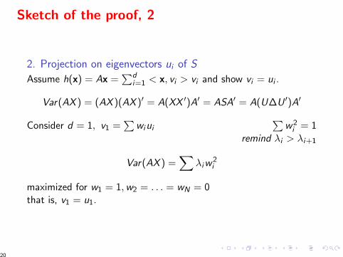
Sketch of the proof, 2
2. Projection on eigenvectors ui of S
Assume h(x) = Ax =∑d
i=1 < x, vi > vi and show vi = ui .
Var(AX ) = (AX )(AX )′ = A(XX ′)A′ = ASA′ = A(U∆U ′)A′
Consider d = 1, v1 =∑
wiui∑
w 2i = 1
remind λi > λi+1
Var(AX ) =∑
λiw2i
maximized for w1 = 1,w2 = . . . = wN = 0that is, v1 = u1.
20
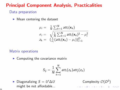
Principal Component Analysis, Practicalities
Data preparation
I Mean centering the dataset
µi = 1N
∑Nk=1 atti (xk)
σi =√
1N
∑Nk=1 atti (xk)2 − µ2
i
zk = ( 1σi
(atti (xk)− µi ))Di=1
Matrix operations
I Computing the covariance matrix
Sij =1
N
N∑k=1
atti (zk)attj(zk)
I Diagonalizing S = U ′∆U Complexity O(D3)might be not affordable...
21
Overview
Introduction
Linear changes of representationPrincipal Component AnalysisRandom projectionsLatent Semantic Analysis
Non linear changes of representation
22
Random projection
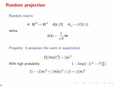
Random matrix
A : IRD 7→ IRd A[d ,D] Ai ,j ∼ N (0, 1)
define
h(x) =1√d
Ax
Property: h preserves the norm in expectation
E [||h(x)||2] = ||x||2
With high probability 1− 2exp{−(ε2 − ε3)d4 }
(1− ε)||x||2 ≤ ||h(x)||2 ≤ (1 + ε)||x||2
23

Random projection
Proof
h(x) = 1√d
Ax
E (||h(x)||2) = 1d E
[∑di=1
(∑Dj=1 Ai ,jXj(x)
)2]
= 1d
∑di=1 E
[(∑Dj=1 Ai ,jXj(x)
)2]
= 1d
∑di=1
∑Dj=1 E [A2
i ,j ]E [Xj(x)2]
= 1d
∑di=1
∑Dj=1
||x||2D
= ||x||2
24
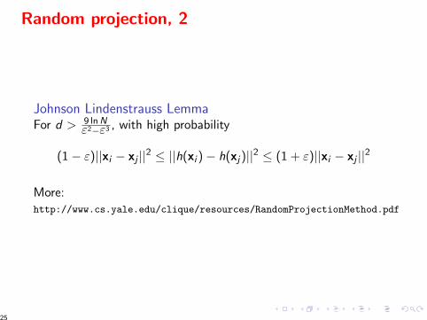
Random projection, 2
Johnson Lindenstrauss LemmaFor d > 9 lnN
ε2−ε3 , with high probability
(1− ε)||xi − xj ||2 ≤ ||h(xi )− h(xj)||2 ≤ (1 + ε)||xi − xj ||2
More:http://www.cs.yale.edu/clique/resources/RandomProjectionMethod.pdf
25

Overview
Introduction
Linear changes of representationPrincipal Component AnalysisRandom projectionsLatent Semantic Analysis
Non linear changes of representation
26

Example
27

Example, followed
28
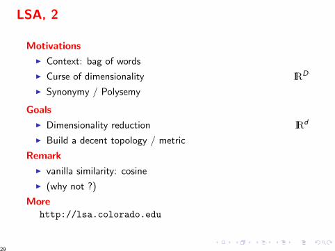
LSA, 2
Motivations
I Context: bag of words
I Curse of dimensionality IRD
I Synonymy / Polysemy
Goals
I Dimensionality reduction IRd
I Build a decent topology / metric
Remark
I vanilla similarity: cosine
I (why not ?)
Morehttp://lsa.colorado.edu
29

LSA, 3
InputMatrice X = mots × documents
Principe1. Changement de base des mots,documents aux concepts2. Reduction de dimension
Difference Analyse en composantes principales
30
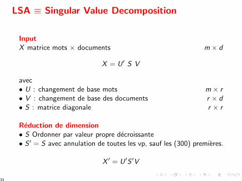
LSA ≡ Singular Value Decomposition
InputX matrice mots × documents m × d
X = U ′ S V
avec• U : changement de base mots m × r• V : changement de base des documents r × d• S : matrice diagonale r × r
Reduction de dimension• S Ordonner par valeur propre decroissante• S ′ = S avec annulation de toutes les vp, sauf les (300) premieres.
X ′ = U ′S ′V
31
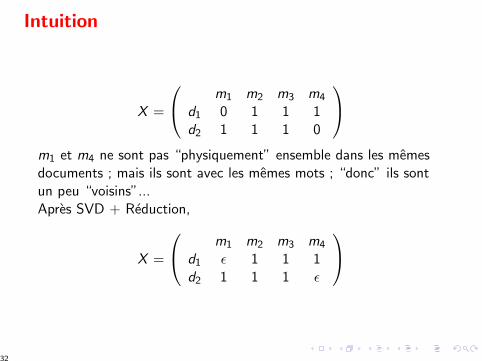
Intuition
X =
m1 m2 m3 m4
d1 0 1 1 1d2 1 1 1 0
m1 et m4 ne sont pas “physiquement” ensemble dans les memesdocuments ; mais ils sont avec les memes mots ; “donc” ils sontun peu “voisins”...Apres SVD + Reduction,
X =
m1 m2 m3 m4
d1 ε 1 1 1d2 1 1 1 ε
32

Algorithme
33
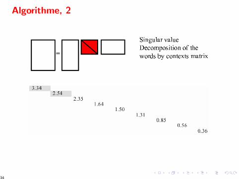
Algorithme, 2
34

Algorithme. 3
35
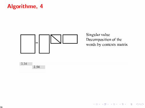
Algorithme, 4
36
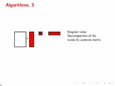
Algorithme, 5
37

Algorithme, 6
38
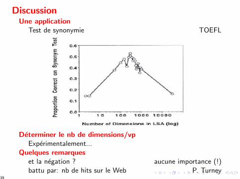
DiscussionUne application
Test de synonymie TOEFL
Determiner le nb de dimensions/vpExperimentalement...
Quelques remarqueset la negation ? aucune importance (!)battu par: nb de hits sur le Web P. Turney
39

Quelques applications
I Educational Text SelectionPermet de selectionner automatiquement des textespermettant d’accroıtre les connaissances de l’utilisateur.
I Essay ScoringPermet de noter la qualite d’une redaction d’etudiant
I Summary Scoring & RevisionApprendre a l’utilisateur a faire un resume
I Cross Language Retrievalpermet de soumettre un texte dans une langue et d’obtenir untexte equivalent dans une autre langue
40

LSA − Analyse en composantes principales
Ressemblances
I Prendre une matrice
I La mettre sous forme diagonale
I Annuler toutes les valeurs propres sauf les plus grandes
I Projeter sur l’espace obtenu
DifferencesACP LSA
Matrice covariance attributs mots × documentsd 2-3 100-300
41
Overview
Introduction
Linear changes of representationPrincipal Component AnalysisRandom projectionsLatent Semantic Analysis
Non linear changes of representation
42

Non-Linear Dimensionality Reduction
Conjecture
Examples live in a manifold of dimension d << D
Goal: consistent projection of the dataset onto IRd
Consistency:
I Preserve the structure of the data
I e.g. preserve the distances between points
43
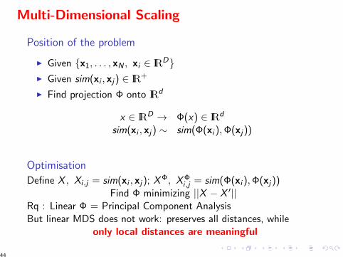
Multi-Dimensional Scaling
Position of the problem
I Given {x1, . . . , xN , xi ∈ IRD}I Given sim(xi , xj) ∈ IR+
I Find projection Φ onto IRd
x ∈ IRD → Φ(x) ∈ IRd
sim(xi , xj) ∼ sim(Φ(xi ),Φ(xj))
Optimisation
Define X , Xi ,j = sim(xi , xj); X Φ, X Φi ,j = sim(Φ(xi ),Φ(xj))
Find Φ minimizing ||X − X ′||Rq : Linear Φ = Principal Component AnalysisBut linear MDS does not work: preserves all distances, while
only local distances are meaningful
44
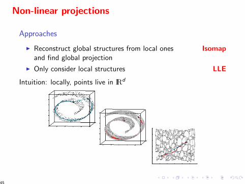
Non-linear projections
Approaches
I Reconstruct global structures from local ones Isomapand find global projection
I Only consider local structures LLE
Intuition: locally, points live in IRd
45
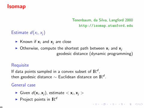
Isomap
Tenenbaum, da Silva, Langford 2000
http://isomap.stanford.edu
Estimate d(xi , xj)
I Known if xi and xj are close
I Otherwise, compute the shortest path between xi and xjgeodesic distance (dynamic programming)
Requisite
If data points sampled in a convex subset of IRd ,then geodesic distance ∼ Euclidean distance on IRd .
General case
I Given d(xi , xj), estimate < xi , xj >
I Project points in IRd
46

Isomap, 2
47

Locally Linear Embedding
Roweiss and Saul, 2000
http://www.cs.toronto.edu/∼roweis/lle/
Principle
I Find local description for each point: depending on itsneighbors
48

Local Linear Embedding, 2
Find neighbors
For each xi , find its nearest neighbors N (i)Parameter: number of neighbors
Change of representation
Goal Characterize xi wrt its neighbors:
xi =∑
j∈N (i)
wi ,jxj with∑
j∈N (i)
wij = 1
Property: invariance by translation, rotation, homothetyHow Compute the local covariance matrix:
Cj ,k =< xj − xi , xk − xi >
Find vector wi s.t. Cwi = 1
49
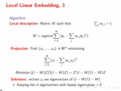
Local Linear Embedding, 3
Algorithm
Local description: Matrix W such that∑
j wi ,j = 1
W = argmin{N∑i=1
||xi −∑j
wi ,jxj ||2}
Projection: Find {z1, . . . , zn} in IRd minimizing
N∑i=1
||zi −∑j
wi ,jzj ||2
Minimize ((I −W )Z )′((I −W )Z ) = Z ′(I −W )′(I −W )Z
Solutions: vectors zi are eigenvectors of (I −W )′(I −W )
I Keeping the d eigenvectors with lowest eigenvalues > 0
50
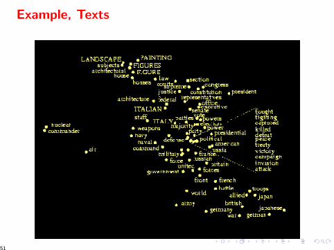
Example, Texts
51
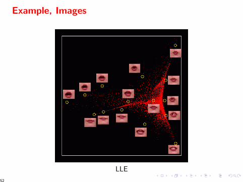
Example, Images
LLE
52
Overview
Introduction
Linear changes of representationPrincipal Component AnalysisRandom projectionsLatent Semantic Analysis
Non linear changes of representation
53
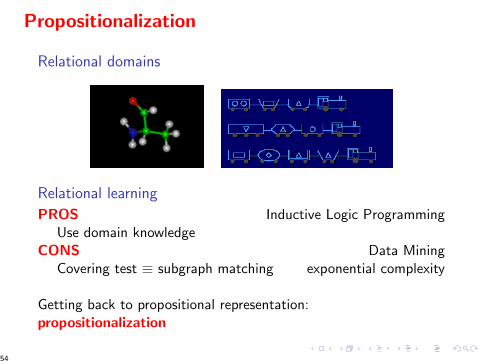
Propositionalization
Relational domains
Relational learning
PROS Inductive Logic ProgrammingUse domain knowledge
CONS Data MiningCovering test ≡ subgraph matching exponential complexity
Getting back to propositional representation:propositionalization
54
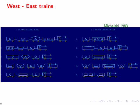
West - East trains
Michalski 1983
55
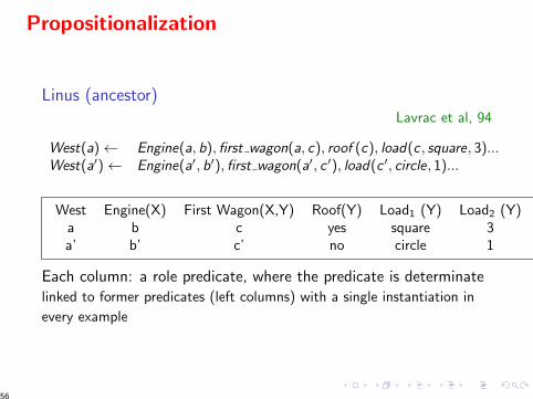
Propositionalization
Linus (ancestor)Lavrac et al, 94
West(a)← Engine(a, b), first wagon(a, c), roof (c), load(c , square, 3)...West(a′)← Engine(a′, b′), first wagon(a′, c ′), load(c ′, circle, 1)...
West Engine(X) First Wagon(X,Y) Roof(Y) Load1 (Y) Load2 (Y)a b c yes square 3a’ b’ c’ no circle 1
Each column: a role predicate, where the predicate is determinatelinked to former predicates (left columns) with a single instantiation in
every example
56
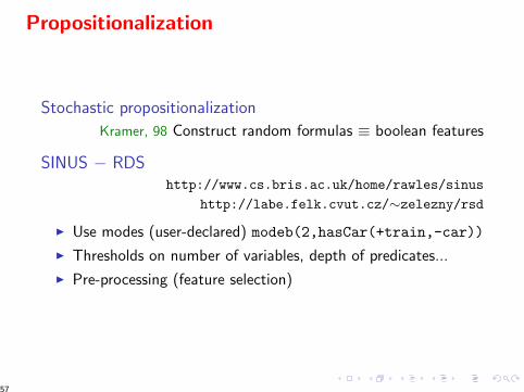
Propositionalization
Stochastic propositionalization
Kramer, 98 Construct random formulas ≡ boolean features
SINUS − RDShttp://www.cs.bris.ac.uk/home/rawles/sinus
http://labe.felk.cvut.cz/∼zelezny/rsd
I Use modes (user-declared) modeb(2,hasCar(+train,-car))
I Thresholds on number of variables, depth of predicates...
I Pre-processing (feature selection)
57
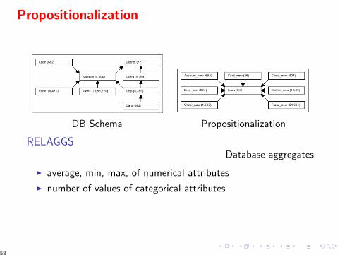
Propositionalization
DB Schema Propositionalization
RELAGGSDatabase aggregates
I average, min, max, of numerical attributes
I number of values of categorical attributes
58
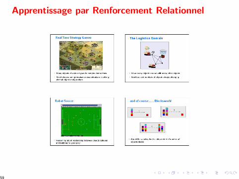
Apprentissage par Renforcement Relationnel
59
Propositionalisation
Contexte variable
I Nombre de robots, position des robots
I Nombre de camions, lieu des secours
Besoin: Abstraire et Generaliser
Attributs
I Nombre d’amis/d’ennemis
I Distance du plus proche robot ami
I Distance du plus proche ennemi
60