L systems

Lila Kari

Department of Mathematics, University of Western Ontario

London, Ontario, N6A 5B7 Canada

Grzegorz Rozenberg

Department of Computer Science, University of Leiden

P.O.Box 9512, NL-2300 RA Leiden, The Netherlands

Arto Salomaa

Department of Mathematics, University of Turku

20 500 Turku, Finland

1 Introduction

1.1 Parallel rewriting

L systems are parallel rewriting systems which were originally introduced in1968 to model the development of multicellular organisms, [L1]. The basic ideasgave rise to an abundance of language-theoretic problems, both mathematicallychallenging and interesting from the point of view of diverse applications. Afteran exceptionally vigorous initial research period (roughly up to 1975; in the book[RSed2], published in 1985, the period up to 1975 is referred to, [RS2], as “whenL was young”), some of the resulting language families, notably the families ofD0L, 0L, DT0L, E0L and ET0L languages, had emerged as fundamental onesin the parallel or L hierarchy. Indeed, nowadays the fundamental L familiesconstitute a similar testing ground as the Chomsky hierarchy when new devices(grammars, automata, etc.) and new phenomena are investigated in languagetheory.

L systems were introduced by Aristid Lindenmayer in 1968, [L1]. The origi-nal purpose was to model the development of simple filamentous organisms. Thedevelopment happens in parallel everywhere in the organism. Therefore, paral-lelism is a built-in characteristic of L-systems. This means, from the point ofview of rewriting, that everything has to be rewritten at each step of the rewrit-ing process. This is to be contrasted to the “sequential” rewriting of phrasestructure grammars: only a specific part of the word under scan is rewrittenat each step. Of course, the effect of parallelism can be reached by several se-

1

quential steps in succession. However, the synchronizing control mechanism ismissing from the customary sequential rewriting devices. Therefore, parallelismcannot be truly simulated by sequential rewriting.

Assume that your only rule is a −→ a2 and you start with the word a3.What do you get? If rewriting is sequential, you can replace one a at a timeby a2, obtaining eventually all words words ai, i ≥ 3. If rewriting is parallel,the word a6 results in one step. It is not possible to obtain a4 or a5 from a3.Altogether you get only the words a3·2i

, i ≥ 0. Clearly, the language

{a3·2i

| i ≥ 0}

is not obtainable by sequential context-free or interactionless rewriting: lettersare rewritten independently of their neighbours. Observe also how the dummyrule a −→ a behaves dramatically differently in parallel and sequential rewriting.In the latter it has no influence and can be omitted without losing anything. Inparallel rewriting the rule a −→ a makes the simulation of sequential rewritingpossible: the “real” rule a −→ a2 is applied to one occurrence of a, and the“dummy” rule a −→ a to the remaining occurrences. Consequently, all wordsai, i ≥ 3, are obtained by parallel rewriting from a3 if both of the rules a −→ a2

and a −→ a are available.The present survey on L systems can by no means be encyclopedic; we do

not even claim that we can exhaust all the main trends. Of the huge bibli-ography concerning L systems we reference only items needed to illustrate oraugment an isue in our presentation. We are fully aware that also some ratherinfluential papers have not been referenced. In the early years of L systemsit was customary to emphasize that the exponential function 2n described theyearly growth in the number of papers in the area. [MRS], published in 1981,was the latest edition of a bibliography on L systems intended to be comprehen-sive. After that nobody has undertaken the task of compiling a comprehensivebibliography which by now would contain at least 5 000 items.

On the other hand, L systems will be discussed also elsewhere in this Hand-book. They form the basic subject matter in the chapter of P.Prusinkiewiczin Volume III but are also covered, for instance, in the chapters by W.KuichG.Paun – A.Salomaa in the present Volume I.

When we write “L systems” or “ET0L languages” without a hyphen, it isnot intentionally vicious ortography. We only follow the practice developedduring the years among the researchers in this field. The main reason for thispractice was that in complicated contexts the hyphen was often misleading. Wewant to emphasize in this connection the notational uniformity followed by theresearchers of L systems, quite exceptional in comparison with most areas ofmathematical research. In particular, the different letters have a well-definedmeaning in the names of the L language families. For instance, it is immediatelyunderstood by everyone in the field what HPDF0L languages are. We will returnto the terminology in Section 2 below.

2

1.2 Callithamnion roseum, a primordial alga

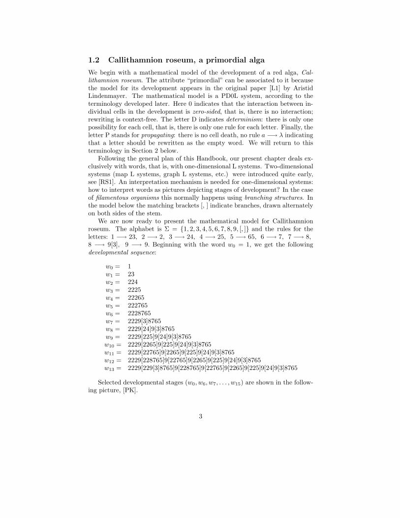
We begin with a mathematical model of the development of a red alga, Cal-lithamnion roseum. The attribute “primordial” can be associated to it becausethe model for its development appears in the original paper [L1] by AristidLindenmayer. The mathematical model is a PD0L system, according to theterminology developed later. Here 0 indicates that the interaction between in-dividual cells in the development is zero-sided, that is, there is no interaction;rewriting is context-free. The letter D indicates determinism: there is only onepossibility for each cell, that is, there is only one rule for each letter. Finally, theletter P stands for propagating: there is no cell death, no rule a −→ λ indicatingthat a letter should be rewritten as the empty word. We will return to thisterminology in Section 2 below.

Following the general plan of this Handbook, our present chapter deals ex-clusively with words, that is, with one-dimensional L systems. Two-dimensionalsystems (map L systems, graph L systems, etc.) were introduced quite early,see [RS1]. An interpretation mechanism is needed for one-dimensional systems:how to interpret words as pictures depicting stages of development? In the caseof filamentous organisms this normally happens using branching structures. Inthe model below the matching brackets [, ] indicate branches, drawn alternatelyon both sides of the stem.

We are now ready to present the mathematical model for Callithamnionroseum. The alphabet is Σ = {1, 2, 3, 4, 5, 6, 7, 8, 9, [, ]} and the rules for theletters: 1 −→ 23, 2 −→ 2, 3 −→ 24, 4 −→ 25, 5 −→ 65, 6 −→ 7, 7 −→ 8,8 −→ 9[3], 9 −→ 9. Beginning with the word w0 = 1, we get the followingdevelopmental sequence:

w0 = 1w1 = 23w2 = 224w3 = 2225w4 = 22265w5 = 222765w6 = 2228765w7 = 2229[3]8765w8 = 2229[24]9[3]8765w9 = 2229[225]9[24]9[3]8765w10 = 2229[2265]9[225]9[24]9[3]8765w11 = 2229[22765]9[2265]9[225]9[24]9[3]8765w12 = 2229[228765]9[22765]9[2265]9[225]9[24]9[3]8765w13 = 2229[229[3]8765]9[228765]9[22765]9[2265]9[225]9[24]9[3]8765

Selected developmental stages (w0, w6, w7, . . . , w15) are shown in the follow-ing picture, [PK].

3

1.3 Life, real and artificial

We conclude this Introduction with some observations that, in our estimation,are rather important in predicting the future developments of L systems. Lsystems were originally introduced to model the development of multicellularorganisms, that is, the development of some form of “real” life. However, therehave been by now numerous applications in computer graphics, where L systemshave been used to depict imaginary life forms, imaginary gardens of L and alsonon-living specimens ranging from toys and birthday cakes to real-estate ads(see, for instance, [PL]). Their utmost simplicity and flexibility to small changestailor-made according to individual wishes make L systems very suitable tomodel phenomena of artificial life.

Artificial life is customarily understood as the study of man-made constructsthat exhibit, in some sense or in some aspects, the behavior of existing livingorganisms. Artificial life extends the traditional biology that is concerned withthe carbon-chain-type of life evolved on Earth. Artificial life tries to synthesizelife-like behavior within computers and other man-made devices. It is alsomore extensive than robotics. Robots are constructed to do some specific tasks,whereas the “creatures” of artificial life are only observed. As often explained,artificial life paints the picture of life-as-it-could-be, contrasted to the picture oftraditional biology about life-as-we-know-it.

It is very difficult to draw a strict border between living and nonliving, an-imate and inanimate. No definition of “life”, satisfactory in a mathematical orcommon sense, has so far been given. Perhaps it is better to view the set of

4

living beings as a fuzzy set rather than to try to define it in crisp mathematicalterms. Another possibility is to give lists of properties typical for living beingsas contrasted to inanimate objects. However, so far none of such lists seems sat-isfactory. Also many individual properties, such as growth, give rise to doubts.Although growth is typical for living beings, it can be observed elsewhere.

However, one feature very characteristic for the architecture of all livingbeings is that life is fundamentally parallel. A living system may consist of mil-lions of parts, all having their own characteristic behavior. However, althougha living system is highly distributed, it is massively parallel.

Thus, any model for artificial life must be capable of simulating parallelism– no other approach is likely to prove viable. Among all grammatical models, Lsystems are by their very essence the most suitable for modeling parallelism. Lsystems may turn out to be even more suitable for modeling artificial life thanreal life.

Indeed, the utmost simplicity of the basic components and the ease of affect-ing changes tailor-made for clarifying a specific issue render L systems ideal formodeling artificial life. A good example is the so-called French Flag Problem:does polarized behavior at the global level imply polarization (that is, nonsym-metric behavior) at the local level? The idea behind this problem (as describedin [H2] and [HR]) comes from a worm with three parts (like the French Flag):head, middle, tail. If one of the ends is cut, the worm grows again the missingpart, head for head and tail for tail. The behavior of the uncut part is polarized– the remaining organism knows which end it assists to grow. However, sucha global behavior can be reached by a fully symmetric local behavior. It canbe modeled by an L system, where the rules for the individual cells are fullysymmetric – there is no distinction between right and left, [HR]. While such aconstruction does not in any way prove that the real-life phenomenon is locallysymmetric – the cells of the worm used in experiments can very well be polar-ized – it certainly constitutes an important fact of artificial life. We can haveliving species with polarized global behavior but with fully symmetric behaviorat the level of individual cells – and possibly having some other features we areinterested in implementing.

Other grammatical models, or grammar-like models such as cellular au-tomata, seem to lack the versatility and flexibility of L systems. It is not easy toaffect growth of the interior parts using cellular automata, whereas L-filamentsgrow naturally everywhere. If you want to make a specific alteration in thespecies you are interested in, then you very often find a suitable L system tomodel the situation. On the other hand, it seems that still quite much post-editing is needed in graphical real-life modeling. The variations of L systemsconsidered so far seem to be too simple to capture some important features ofreal-life phenomena. We now proceed to present the most common of thesevariations, beginning with the basic ones.

5

2 The world of L, an overview

2.1 Iterated morphisms and finite substitutions: D0L and

0L

We will now present the fundamentals of L systems and their basic properties.Only very few notions of language theory are needed for this purpose. We followSection 2.1 of Chapter 1 in this Handbook as regards the core terminology aboutletters, words and languages. The most important language-theoretic notionneeded below will be a finite substitution over an alphabet Σ, as well as itsspecial cases.

Definition. A finite substitution σ over an alphabet Σ is a mapping ofΣ∗ into the set of all finite nonempty languages (possibly over an alphabet ∆different from Σ) defined as follows. For each letter a ∈ Σ, σ(a) is a finitenonempty language, σ(λ) = λ and, for all words w1, w2 ∈ Σ∗,

σ(w1w2) = σ(w1)σ(w2).

If none of the languages σ(a), a ∈ Σ, contains the empty word, the substi-tution σ is referred to as λ-free or nonerasing. If each σ(a) consists of a singleword, σ is called a morphism. We speak also of nonerasing and letter-to-lettermorphisms.2

Some clarifying remarks are in order. Morphisms were earlier called ho-momorphisms – this fact is still reflected by the notations h and H used inconnection with morphisms. Usually in our considerations the target alphabet∆ equals the basic alphabet Σ – this will be the case in the definition of D0Land 0L systems. Then we speak briefly of a finite substitution or morphism onthe alphabet Σ. In the theory of L systems letter-to-letter morphisms are cus-tomarily called codings; weak codings are morphisms mapping each letter eitherto a letter or to the empty word λ. Codings in this sense should not be confusedwith codes discussed elsewhere in this Handbook, also in Section 6 below.

By the above definition a substitution σ is applied to a word w by rewritingevery letter a of w as some word from σ(a). Different occurrences of a maybe rewritten as different words of σ(a). However, if σ is a morphism theneach σ(a) consists of one word only, which makes the rewriting deterministic.It is convenient to specify finite substitutions by listing the rewriting rules orproductions for each letter, for instance,

a −→ λ, a −→ a2, a −→ a7,

this writing being equivalent to

σ(a) = {λ, a2, a7}.

Now, for instance,

σ(a2) = σ(a)σ(a) = {λ, a2, a4, a7, a9, a14}.

6

Similarly, the substitution (in fact, a morphism) defined by

σ1(a) = {b}, σ1(b) = {ab}, Σ = {a, b},

can be specified by listing the rules

a −→ b, b −→ ab.

In this case, for any word w, σ1(w) consists of a single word, for instance,

σ1(a2ba) = {b2ab2} = b2ab2,

where the latter equality indicates only that we often identify singleton sets withtheir elements.

The above results for σ(a2) and σ1(a2ba) are obtained by applying the rules

in parallel: every occurrence of every letter must be rewritten. Substitutionsσ (and, hence, also morphisms) are in themselves parallel operations. Anapplication of σ to a word w means that something happens everywhere in w.No part of w can remain idle except that, in the presence of the rule a −→ a,occurences of a may remain unchanged.

Before our next fundamental definition, we still want to extend applicationsof substitutions (and, hence, also morphisms) to concern also languages. This isdone in the natural “additive” fashion. By definition, for all languages L ⊆ Σ∗,

σ(L) = {u| u ∈ σ(w), for some w ∈ L}.

Definition. A 0L system is a triple G = (Σ, σ, w0), where Σ is an alphabet,σ is a finite substitution on Σ, and w0 (referred to as the axiom) is a word overΣ. The 0L system is propagating or a P0L system if σ is nonerasing. The 0Lsystem G generates the language

L(G) = {w0} ∪ σ(w0) ∪ σ(σ(w0)) ∪ . . . =⋃

i≥0

σi(w0). 2

Consider, for instance, the 0L system

MISS3 = ({a}, σ, a) with σ(a) = {λ, a2, a5}.

(Here and often in the sequel we express in the name of the system some charac-teristic property, rather than using abruptly an impersonal G– notation.) Thesystem can be defined by simply listing the productions

a −→ λ, a −→ a2, a −→ a5

and telling that a is the axiom. Indeed, both the alphabet Σ and the substitutionσ can be read from the productions. (We disregard the case, where Σ contains

7

letters not appearing in the productions.) L systems are often in the sequeldefined in this way, by listing the productions.

Going back to the system MISS3, we obtain from the axiom a in one “deriva-tion step” each of the words λ, a2, a5. Using customary language-theoretic no-tation, we denote this fact by

a =⇒ λ, a =⇒ a2, a =⇒ a5.

A second derivation step gives nothing new from λ but gives the new wordsa4, a7, a10 from a2 and the additional new words a6, a8, a9, a11, a12, a13, a14,a15, a16, a17, a19, a20, a22, a25 from a5. In fact,

a5 =⇒ ak iff k = 2i + 5j, i + j ≤ 5, i ≥ 0, j ≥ 0.

(Thus, we use the notation w =⇒ u to mean that u ∈ σ(w).) A third derivationstep produces, in fact in many different ways, the missing words a18, a21, a23,a24. Indeed, it is straightforward to show by induction that

L(MISS3) = {ai| i 6= 3}.

Let us go back to the terminology used in defining L systems. The letterL comes from the name of Aristid Lindenmayer. The story goes that Aristidwas so modest himself that he said that it comes from “languages”. The num-ber 0 in “0L system” indicates that interaction between individual cells in thedevelopment is zero-sided, the development is without interaction. In language-theoretic terms this means that rewriting is context-free. The system MISS3 isnot propagating, it is not P0L. However, it is a unary 0L system, abbreviatedU0L system: the alphabet consists of one letter only. The following notion willbe central in our discussions.

Definition. A 0L system (Σ, σ, w0) is deterministic or a D0L system iff σis a morphism. 2

Thus, if we define a D0L system by listing the productions, there is exactlyone production for each letter. This means that rewriting is completely de-terministic. We use the term propagating, or a PD0L system, also here: themorphism is nonerasing. The L system used in Section 1.2 for modeling Cal-lithamnion roseum was, in fact, a PD0L system.

D0L systems are the simplest among L systems. Although most simple,D0L systems give a clear insight into the basic ideas and techniques behind Lsystems and parallel rewriting in general. The first L systems used as modelsin developmental biology, as well as most of the later ones, were in fact D0Lsystems. From the point of view of artificial life, creatures modeled by D0Lsystems have been called, [S7], “Proletarians of Artificial Life”, briefly PAL’s. Inspite of the utmost simplicity of the basic definition, the theory of D0L systems isby now very rich and diverse. Apart from providing tools for modeling real andartificial life, the theory has given rise to new deep insights into language theory

8

(in general) and into the very basic mathematical notion of an endomorphismon a free monoid (in particular), [S5]. At present still a wealth of problems andmysteries remains concerning D0L systems.

Let G = (Σ, h, w0) be a D0L system – we use the notation h to indicate thatwe are dealing with a (homo)morphism. The system G generates its languageL(G) in a specific order, as a sequence:

w0, w1 = h(w0), w2 = h(w1) = h2(w0), w3, . . .

We denote the sequence by S(G). Thus, in connection with a D0L system G, wespeak of its language L(G) and sequence S(G). Indeed, D0L systems were thefirst widely studied grammatical devices generating sequences. We now discussfive examples, paying special attention to sequences. All five D0L systems arepropagating, that is, PD0L systems. The first one is also unary, that is, aUPD0L system.

Consider first the D0L system EXP2 with the axiom a and rule a −→ a2.It is immediate that the sequence S(EXP2) consists of the words a2i

, i ≥ 0, inthe increasing length order. Secondly, consider the D0L system LIN with theaxiom ab and rules a −→ a, b −→ ab. Now the sequence S(LIN) consists of thewords aib, i ≥ 1, again in increasing length order. The notation LIN refers tolinear growth in word length: the j’th word in the sequence is of length j + 2.(Having in mind the notation w0, w1, w2, we consider the axiom ab to be the0th word etc.)

Our next D0L system FIB has the axiom a and rules a −→ b, b −→ ab. Thefirst few words in the sequence S(FIB) are

a, b, ab, bab, abbab, bababbab.

From the word ab on, each word results by catenating the two precedingones. Let us establish inductively this claim,

wn = wn−2wn−1, n ≥ 2.

Denoting by h the morphism of the system FIB, we obtain using the definitionof h:

wn = hn(a) = hn−1(h(a)) = hn−1(b) = hn−2(h(b)) =

= hn−2(ab) = hn−2(a)hn−2(b) = hn−2(a)hn−2(h(a)) =

= hn−2(a)hn−1(a) = wn−2wn−1.

The claim established shows that the word lengths satisfy the equation

|wn| = |wn−2| + |wn−1|, n ≥ 2.

Hence, the length sequence is the well-known Fibonacci sequence 1, 1, 2, 3, 5,8, 13, 21, 34, ...

9

The D0L system SQUARES has the axiom a and rules

a −→ abc2, b −→ bc2, c −→ c.

The sequence S(SQUARES) begins with the words

a, abc2, abc2bc2c2, abc2bc2c2bc2c2c2.

Denoting again by wi, i ≥ 0, the words in the sequence, it is easy to verifyinductively that

|wi+1| = |wi| + 2i + 3, for all i ≥ 0.

This shows that the word lengths consist of the consecutive sequence: |wi| =(i+1)2, for all i ≥ 0. Similar considerations show that the D0L system CUBESwith the axiom a and productions

a −→ abd6, b −→ bcd11, c −→ cd6, d −→ d

satisfies |wi| = (i + 1)3, for all i ≥ 0.Rewriting being deterministic gives rise to certain periodicities in the D0L

sequence. Assume that some word occurs twice in a sequence: wi = wi+j , forsome i ≥ 0 and j ≥ 1. Because of the determinism, the words following wi+j

coincide with those following wi, in particular,

wi = wi+j = wi+2j = wi+3j = . . .

Thus, after some “initial mess”, the words start repeating periodically in thesequence. This means that the language of the system is finite. Conversely, ifthe language is finite, the sequence must have a repetition. This means thatthe occurrence of a repetition in S(G) is a necessary and sufficient condition forL(G) being finite. Some other basic periodicity results are given in the followingtheorem, for proofs see [HR], [Li2], [RS1]. The notation alph(w) means theminimal alphabet containing all letters occurring in w, prefk(w) stands for theprefix of w of length k (or for w itself if |w| < k), sufk(w) being similarly defined.

Theorem 2.1. Let wi, i ≥ 0, be the sequence of a D0L system G =(Σ, h, w0). Then the sets Σi = alph(wi), i ≥ 0, form an ultimately periodicsequence, that is, there are numbers p > 0 and q ≥ 0 such that Σi = Σi+p holdsfor every i ≥ q. Every letter occurring in some Σi occurs in some Σj with j ≤card(Σ) − 1. If L(G) is infinite then there is a positive integer t such that, forevery k > 0, there is an n > 0 such that, for all i ≥ n and m ≥ 0,

prefk−1(wi) = prefk−1(wi+mt) and suf(wi) = sufk−1(wi+mt).2

Thus, both prefixes and suffixes of any chosen length form an ultimatelyperiodic sequence. Moreover, the period is independent of the length chosen;only the initial mess depends on it.

10

Definition. An infinite sequence of words wi, i ≥ 0, is locally catenative iff,for some positive integers k, i1, . . . ik and q ≥ max(i1, . . . , ik),

wn = wn−i1 . . . wn−ikwhenever n ≥ q.

A D0L system G is locally catenative iff the sequence S(G) is locally catenative.

2

Locally catenative D0L systems are very important both historically andbecause of their central role in the theory of D0L systems: their study hasopened up new branches of the theory. A very typical example of a locallycatenative D0L system is the system FIB discussed above.

Also the system EXP2 is locally catenative: the sequence S(EXP2) satisfies

wn = wn−1wn−1 for all n ≥ 1.

A celebrated problem, still open, is to decide whether or not a given D0L systemis locally catenative. No general algorithm is known, although the problem hasbeen settled in some special cases, for instance, when an upper bound is knownfor the integers i1, . . . ik, as well as recently for binary alphabets, [Ch].

An intriguing problem is the avoidability or unavoidability of cell death:to what extent are rules a −→ λ necessary in modeling certain phenomena?What is the real difference between D0L and PD0L systems and between 0Land P0L systems? There are some straightforward observations. The wordlength can never decrease in a PD0L sequence, and a P0L language cannotcontain the empty word. We will see in the sequel, especially in connection withgrowth functions, that there are remarkable differences between D0L and PD0Lsystems. The theory of D0L systems is very rich and still in many respectspoorly understood.

As an example of the necessity of cell death, consider the D0L systemDEATHb with the axiom ab2a and rules

a −→ ab2a, b −→ λ.

The sequence S(DEATHb) consists of all words (ab2a)2i

, i ≥ 0, in the increasingorder of word length. We claim that the language L consisting of these wordscannot be generated by any PD0L system G. Indeed, ab2a would have to be theaxiom of such a G, and ab2a =⇒ ab2aab2a would have to be the first derivationstep. This follows because no length-decrease is possible in S(G). The twooccurrences of a in ab2a must produce the same subword in ab2aab2a. Thishappens only if the rule for a is one of the following: a −→ λ, a −→ ab2a,a −→ a. The first two alternatives lead to non-propagating systems. Butalso the last alternative is impossible because no rule for b makes the stepb2 =⇒ b2aab2 possible. We conclude that it is not possible to generate thelanguage L(DEATHb) using a PD0L system.

11

A slight change in DEATHb makes such a generation possible. Consider theD0L system G1 with the axiom aba and rules a −→ aba, b −→ λ. Now thePD0L system G2 with the axiom aba and rules a −→ a, b −→ baab generatesthe same sequence, S(G1) = S(G2).

We say that two D0L systems G1 and G2 are sequence equivalent iff S(G1) =S(G2). They are language equivalent, briefly equivalent, iff L(G1) = L(G2). In-stead of D0L systems, these notions can be defined analogously for any otherclass of L systems – sequence equivalence of course only for systems generatingsequences. The two systems G1 and G2 described in the preceding paragraph areboth sequence and language equivalent. Clearly, sequence equivalence implieslanguage equivalence but the reverse implication is not valid. Two D0L systemsmay be (language) equivalent without being sequence equivalent, they can gen-erate the same language in a different order. A simple example is provided bythe two systems

({a, b}, {a −→ b2, b −→ a}, b) and ({a, b}, {a −→ b, b −→ a2}, a).

Among the most intriguing mathematical problems about L systems is theD0L equivalence problem: construct an algorithm for deciding whether or nottwo given D0L systems are equivalent. Equivalence problem is a fundamentaldecision for any family of generative devices: decide whether or not two givendevices in the family generate the same language. For D0L systems one canconsider, in addition, the sequence equivalence problem: Is S(G1) = S(G2),given D0L systems G1 and G2? The D0L equivalence problems were celebratedopen problems for most of the 70’s. They were often referred to as the mostsimply stated problems with an open decidability status. We will return to themand related material in Section 4. It was known quite early, [N], that a solutionto the D0L sequence equivalence problem yields a solution to the D0L languageequivalence problem, and vice versa.

2.2 Auxiliary letters and other auxiliary modifications

A feature very characteristic for D0L systems and 0L systems is that you haveto accept everything produced by the machinery. You have the axiom and therules, and you want to model some phenomenon. You might want to excludesomething that comes out of from the axiom by the rules because it is aliento the phenomenon, does not fit it. This is not possible, you have to includeeverything. There is no way of hiding unsuitable words. Your D0L or 0L modelshave no filtering mechanism.

It is customary in formal language theory to use various filtering mecha-nisms. Not all words obtained in derivations are taken to the language but theterminal language is somehow “squeezed” from the set of all derived words. Themost typical among such filtering mechanisms, quite essential in grammars inthe Chomsky hierarchy, is the use of nonterminal letters. An occurrence of a

12

nonterminal in a word means that the word is not (maybe not yet) acceptable.The generated language contains only words without nonterminals. Thus, thelanguage directly obtained is filtered by intersecting it with Σ∗

T , where ΣT is thealphabet consisting of terminal letters. This gives the possibility of rejecting (atleast some) unsuitable words.

The same mechanism, as well as many other filters, can be used also withL systems. However, a word of warning is in order. The original goal was tomodel the development of a species, be it real or artificial. Each word generatedis supposed to represent some stage in the development. It would be ratherunnatural to exclude some words and say that they do not represent properstages of the development! This is exactly what filtering with nonterminalsdoes.

However, this objection can be overruled because the following justificationcan be given. Some other squeezing mechanisms, notably codings (that is, letter-to-letter morphisms), can be justified from the point of view of developmentalmodels: more careful experiments or observations can change the interpretationof individual cells, after which the cells are assigned new names. This amountsto applying a letter-to-letter morphism to the language. A rather amazing resultconcerning parallel rewriting, discussed below in more detail, is that coding is inimportant cases, [ER1], equivalent to the use of nonterminals in the sense thatthe same language is obtained, and the transition from one squeezing mechanismto the other is effective. By this result, also the use of nonterminals is well-motivated.

The letter E (“extended”) in the name of an L system means that the useof nonterminals is allowed. Thus, an E0L system is a 0L system, where thealphabet is divided into two disjoint parts, nonterminals and terminals. E0Land 0L systems work in the same way but only words over the terminal alphabetare in the language of an E0L system. Thus, an E0L system G can be also viewedas a 0L system, where a subalphabet ΣT is specified and the language of the 0Lsystem is intersected with Σ∗

T to get the language of the E0L system.The following E0L system SYNCHRO is very instructive. In our notation,

capital letters are nonterminals and small letters terminals. The axiom ofSYNCHRO is ABC, and the rules as follows:

A −→ AA′ A −→ a A′ −→ A′ A′ −→ a a −→ FB −→ BB′ B −→ b B′ −→ B′ B′ −→ b b −→ FC −→ CC′ C −→ c C′ −→ C′ C′ −→ c c −→ FF −→ F

It is easy to verify that

L(SYNCHRO) = {anbncn| n ≥ 1}.

This follows because our E0L system is synchronized in the sense that all ter-minals must be reached simultaneously. Otherwise, the failure symbol F neces-sarily comes to the word and can never be eliminated. The language obtained

13

is a classical example in language theory: a context-sensitive language that isnot context-free.

Filtering mechanisms provide families of L languages with a feature very de-sirable both language-theoretically and mathematically: closure under variousoperations. Without filtering, the “pure” families, such as the families of 0Land D0L languages, have very weak closure properties: most of the customarylanguage-theoretic operations may produce languages outside the family, start-ing with languages in the family. For instance, L = {a, a3} is the union of two0L languages. However, L itself is not 0L, as seen by a quick exhaustive searchover the possible axioms and rules.

We refer the reader to the preceding chapter in this Handbook for a moredetailed discussion concerning the following definition. In particular, the sixoperations listed are not arbitrary but exhaust the “rational” operations inlanguage theory.

Definition. A family L of languages is termed a full AFL (“abstract familyof languages”) iff L is closed under each of the following operations: union,catenation, Kleene star, morphism, inverse morphism, intersection with regularlanguages. The family L is termed and anti-AFL iff it is closed under none ofthe operations above. 2

Most of the following theorem can be established by exhibiting suitable ex-amples. [RS1] should be consulted, especially as regards the nonclosure of E0Llanguages under inverse morphisms.

Theorem 2.2. The family of 0L languages is an anti-AFL, and so is thefamily of D0L languages. The family of E0L languages is closed under all AFLoperations except inverse morphism. 2

Theorem 2.2 shows clearly the power of the E-mechanism in transforming afamily of little structure (in the sense of weak closure properties) into a struc-turally strong family. The power varies from L family to another. The differencebetween D0L and ED0L languages is not so big. The periodicity result of Theo-rem 2.1 concerning alphabets holds also for ED0L sequences and, thus, the wordsthat are filtered out occur periodically in the sequence, which is a considerablerestriction.

We now mention other filtering mechanisms. The H-mechanism means tak-ing a morphic image of the original language. Consider the case that the orig-inal language is a 0L language. Thus, let G = (Σ, σ, w0) be a 0L system andh : Σ∗ −→ ∆∗ a morphism. (It is possible that the target alphabet ∆ equalsΣ.) Then h(L(G)) is an H0L language. The HD0L languages are defined anal-ogously.

The N-mechanism refers similarly to nonerasing morphisms. Thus, N0Llanguages are of the form h(L(G)) above, with the additional assumption thath is nonerasing. The C-mechanisms refers to codings and W-mechanism to weakcodings.

A further variation of L systems consists of having a finite set of axioms –instead of only one axiom as we have had in our definitions so far. This variation

14

is denoted by including the letter F in the name of the system. Thus, every finitelanguage L is an F0L language: we just let L be the set of axioms in an F0Lsystem, where the substitution is the identity.

When speaking of language families, we denote the family of E0L languagessimply by E0L, and similarly with other families. Consider the family D0L. Wehave introduced five filtering mechanisms: E, H, N, C, W. This gives six possibil-ities – either some filtering or the pure family. For each of the six possibilities,we may still add one or both of the letters P and F, indicating that we aredealing with the propagating or finite-axiom variant. This gives altogether 24families. The following remarkable theorem gives an exhaustive characterizationof the mutual relashionship between these 24 families. That such a complicatedhierarchy is completely understood is a rather rare situation in language theory.Many of the proofs are rather involved – we return to a tricky question in Section3. Most of the results are originally from [NRSS], see also [RS1]. In comparingthe families, we follow the λ-convention: two languages are considered equal ifthey differ by the empty word only. Otherwise, propagating families would beautomatically different from nonpropagating ones.

Theorem 2.3. The following diagram characterizes mutual relations be-tween deterministic L families. Arrows denote strict inclusion. Families notconnected by a path are mutually incomparable.

HD0L = WD0L =

= HPD0L = WPD0L =

= HDF0L = WDF0L =

= HPDF0L = WPDF0L

= NDF0L = CDF0L

= NPDF0L = CPDF0L

ND0L = NPD0L = CD0L EDF0L

CPD0L ED0L DF0L EPDF0L

EPD0L D0L PDF0L

PD0L

15

In the nondeterministic case there is much more collapse in the hierarchybecause the C-mechanism has in most cases the same generative capacity as theE-mechanism. (In the deterministic case the former is much stronger.) A rathersurprising fact in the nondeterministic case is that, although E0L = C0L, CP0Lis properly contained in EP0L, which is the opposite what one would expectknowing the deterministic case. The key results are given in the next theorem,[NRSS] and [RS1].

Theorem 2.4. Each of the following families equals E0L:

E0L = C0L = N0L = W0L = H0L = NP0L = EP0L = WP0L =HP0L = EF0L = CF0L = NF0L = WF0L = HF0L = EPF0L =NPF0L = WPF0L = HPF0L.

The family E0L lies strictly between context-free and context-sensitive languagesand contains properly the mutually incomparable families CP0L and F0L. 2

Thus, the family E0L contains properly the family of context-free languages.This fact follows because a context-free grammar can be transformed into anE0L system, without affecting the language, by adding the production x −→ xfor each letter x. That the containment is proper can be seen by consideringthe language generated by the E0L system SYNCHRO. This fact should becontrasted with the fact that most finite languages are outside the family of 0Llanguages.

It is customary in language theory to try to reduce grammars into normalforms, that is, to show that every grammar can be replaced by an equivalent(generating the same language) grammar possessing some desirable properties.The following theorem, [RS1], is an illustration of such a reduction for L systems.Observe that the special property of the E0L system SYNCHRO concerningterminals is, in fact, a general property of E0L languages.

Theorem 2.5. Every E0L language is generated by an E0L system satisfy-ing each of the following conditions: (i) The only production for each terminalletter a is a −→ F , where F is a nonterminal having F −→ F as the only pro-duction. (ii) The axiom is a single nonterminal not occurring on the right sideof any production. (iii) The right side of every production is either a terminalword or consists only of nonterminals. (iv) A terminal word is reachable fromevery nonterminal apart from F (and the axiom if the language is empty).2

Usually it is difficult to show that a given language is not in a given family,because, in principle, one has to go through all the devices defining languagesin the family. E0L languages possess certain combinatorial properties and, con-sequently, a language not having those properties cannot be an E0L language,[RS1]. For instance, the language

{ambnam| 1 ≤ m ≤ n}

is not an E0L language. It is very instructive to notice that the languages

{ambnam| 1 ≤ n ≤ m} and {ambnam| m, n ≥ 1}

16

are E0L languages. Finally, the language

{a3n

| n ≥ 1} ∪ {bncndn| n ≥ 1}

is an EP0L language but not a CP0L language.

2.3 Tables, interactions, adults, fragmentation

A feature very characteristic for parallel rewriting is the use of tables, [R1], [R2].A table is simply a set of rewriting rules. A system has several tables, alwaysfinitely many. It is essential that, at each step of the rewriting process, alwaysrules from the same table must be used. This reflects the following state ofaffairs in modeling the development of organisms, real or artificial. There maybe different conditions of the environment (day and night, varying heat, varyinglight, pollution, etc.) or different developmental stages, where it is importantto use different rules. Then we consider all sets of rules, tables, obtained in thisfashion. Observe that tables do not make sense in sequential rewriting. Becauseonly one rule is used at each derivation step, it suffices to consider the total setof rules. We now define the variations of 0L and D0L systems, resulting byaugmenting the system with tables.

Definition. A T0L system is a triple G = (Σ, S, w0), where S is a finiteset of finite substitutions such that, for each σ ∈ S, the triple (Σ, σ, w0) is a 0Lsystem. The language of the T0L system, L(G), consists of w0 and of all wordsin all languages σ1 . . . σk(w0), where k ≥ 1 and each σi belongs to S – some ofthe σi’s may also coincide. If all substitutions in S are, in fact, morphisms thenG is deterministic or a DT0L system. 2

Thus, D indicates that all substitutions (all tables) are deterministic. How-ever, according to the definition above, there is no control in the use of thetables – the tables may be used in an arbitrary order and multitude. Thus, aDT0L language is not generated in a sequence. A definite sequence results onlyif the order in the use of the tables is specified in a unique way.

The letter F has the same meaning as before: finitely many axioms insteadof only one axiom. Also the filtering mechanisms E, H, C, N, W are the sameas before – we will use them below without further explanations.

Following our earlier practice, we will define a T0L system by specifyingthe axiom and each table, a table being a set of productions included in brack-ets to indicate that they belong together. There are no restrictions, the sameproduction may appear in several tables.

As an example consider the DT0L system PAL with the axiom a and twotables

Td = [a −→ b, b −→ b2, c −→ a] and Tn = [a −→ c, b −→ ac, c −→ c].

(The indices d and n come from “day” and “night”, the meaning will becomeclear below.) Instead of a linear sequence, derivations can be represented as atree:

17

a

b

b2 ac

b4 (ac)2 ba c2

b8 (ac)4 (ba)2 c4 b3 ac2 a2

b16 (ac)8 (ba)4 c8 b6 (ac2)2 a4 (ac)3 ba2 c3

Here the branch indicates which of the tables was used: the left descendantresults from an application of Td, the right descendant from an application of Tn.If a descendant is not marked down (like a and c on the third level), it indicatesthat it occurrs already at an earlier level. The continuation can, therefore, beignored if one is only interested in determining the language. The left extremityof the tree contains the powers b2i

, i ≥ 0. However, all powers bi, i ≥ 1, occursomewhere in the tree and so do all powers ai and ci, i ≥ 1. This is seen asfollows. Observe first that, for all i ≥ 0, bai+1 results from bai by applying firstTn, then Td. Now from bai the word bi+2 results by applying Td, the word ci+2

by applying Tn twice, and the word ai+2 from ci+2 by Td.Although seemingly simple, PAL has a rich structure. An interested reader

should have no difficulties in specifying L(PAL) explicitly.) If the order of theapplication of the tables is given, a unique sequence of words results. One mightvisualize the two tables as giving rules for the day and night. The alternation is

18

the natural order of application: TdTnTdTnTd . . . (we agree that we begin withTd). Another possibility is to consider “eternal daylight” (only Td is used) or“eternal night”. Let us still make free the choice of the axiom: instead of theaxiom a, we have an arbitrary nonempty word w over {a, b, c} as the axiom.(Sometimes the term L scheme, instead of an L system, is used to indicatethat the axiom is not specified.) Denote by DAY-AND-NIGHT-PAL(w), DAY-PAL(w), NIGHT-PAL(w) the modifications of PAL thus obtained. Each ofthem generates a specific sequence of words. In fact, DAY-PAL(w) and NIGHT-PAL(w) are PD0L systems, whereas DAY-AND-NIGHT-PAL(w) can be viewedas a CPD0L system. For w = abc, the sequences look as follows.

DAY-NIGHT : abc, b3a, (ac)3c, (ba)3a, (ac2)3c, (ba2)3a,(ac3)3c, (ba3)3a, (ac4)3c, (ba4)3a, . . .

DAY : abc, b3a, b7, b14, b28, . . .NIGHT : abc, cac2, c4, c4, . . .

Definition. For an infinite sequence wi, i ≥ 0, of words, the functionf(n) = |wn| (mapping the set of nonnegative integers into itself) is termed thegrowth function of the sequence.2

Thus, for NIGHT-PAL(abc), f(0) = 3, f(n) = 4 for n ≥ 1. For DAY-

PAL(abc), f(0) = 3, f(1) = 4, f(i + 2) = 27·2i

for i ≥ 0. Finally, for DAY-NIGHT-PAL(abc), f(0) = 3, f(1) = 4, f(2i) = f(2i + 1) = 3i + 1 for i ≥ 1.

Thus, the three growth functions possess, respectively, the property of beingbounded from above by a constant, exponential or linear. In fact, the growthfunction of any NIGHT-PAL(w) (resp. DAY-PAL(w), DAY-NIGHT-PAL(w))is bounded from above by a constant (resp. exponential, linear). We will returnto this matter in Section 5, where growth functions will be discussed.

The following two theorems summarize results concerning mutual relashion-ships between “table families”, [NRSS], [RS1]. The first of the theorems dealswith deterministic families, and the second with nondeterministic families.

Theorem 2.6. The following inclusions and equalities hold:DT0L ⊂ CDT0L= NDT0L= EDT0L= WDT0L= HDT0L,

PDT0L ⊂ CPDT0L ⊆ NPDT0L ⊆ EPDT0L= WPDT0L= HPDT0L,

DTF0L ⊂ CDTF0L= NDTF0L= EDTF0L= WDTF0L= HDTF0L,

PDTF0L⊂ CPDTF0L⊆ NPDTF0L ⊆ EPDTF0L= WDPTF0L= HPDTF0L.

19

The “pure” families (without any filtering) satisfy the following inclusion dia-gram:

DTF0L

DT0L PDTF0L

PDT0L

2

Theorem 2.7. Each of the following families equals ET0L:ET0L= CT0L= NT0L= WT0L= HT0L=

= NPT0L= EPT0L= WPT0L= HPT0L== CTF0L= NTF0L= ETF0L= WTF0L= HTF0L= NPTF0L= EPTF0L= WPTF0L= HPTF0L

The families E0L, TF0L and CPT0L= CPTF0L are all stricly included inET0L. 2

The family ET0L is the largest widely studied L family, where rewriting iscontext-free (no cell interactions are present). It is also very pleasing mathe-matically and has strong closure properties. (It is, however, not closed underthe shuffle operation.) It was observed already in the early 70’s that ET0L iscontained in the family of indexed languages (see the preceding chapter of thisHandbook for a description of indexed languages and see [En] for more generalhierarchies) and, consequently, facts concerning indexed languages hold also forET0L languages. The facts in the following theorem can be established rathereasily.

Theorem 2.8. The family ET0L is a full AFL, whereas the family T0Lis an anti-AFL. Every ET0L language is generated by an ET0L system withtwo tables. Every ET0L language is generated by an ET0L system such thata −→ F is the only rule in every table for every terminal a, and F −→ F is theonly rule in every table for the nonterminal F . 2

The two normal form results stated in Theorem 2.8, the two-table condi-tion and synchronization, cannot always be reached simultaneously. A numberof deep combinatorial results, [RS1], can be established for EDT0L and ET0L

20

languages. Using such results, relatively simple examples can be given of lan-guages not in the families. Let Σ contain at least two letters and k ≥ 2 be afixed integer. Then neither of the languages

{w ∈ Σ∗| |w| = kn, n ≥ 0} and {w ∈ Σ∗| |w| = nk, n ≥ 0}

is in EDT0L. The 0L system with the axiom a and rules

a −→ ab, b −→ bc, b −→ bd, c −→ c, d −→ d

generates a language not in EDT0L. None of the languages

{(abn)m| 1 ≤ m ≤ n}, {(abn)m| 1 ≤ n ≤ m},

{(abn)m| 1 ≤ m = n}, {w ∈ {a, b}∗| |w|b = 2|w|a}

is in ET0L. Here |w|x denotes the number of occurrences of the letter x in w.In the remainder of this subsection 2.3 we survey briefly some areas in

the theory of L systems that are important both historically and language-theoretically in the sense that they have built bridges between sequential andparallel rewriting. Our exposition will be informal. More details can be foundin [RS1], [HWa], [RRS].

In all L systems discussed so far the individual cells develop without anyinteraction with their neighbours. In language-theoretic terms, rewriting hasbeen context-free. We now discuss L systems with interactions, IL sysetms.First some terminology.

In an (m, n)L system, m, n ≥ 0, the rules look like

(α, a, β) −→ w, |α| = m, |β| = n.

This means that, between the words α and β, the letter a can be rewrittenas the word w. Also now, parallelism applies: all letters must be rewrittensimultaneously. In order to get sufficiently many letters on both sides of anygiven letter, the whole rewriting takes place between “environment symbols” #,m of them to the left and n to the right. The rules have to be provided also forthe case that some prefix of α or suffix of β consists of #’s.

The IL system is a collective name for all (m, n)L systems. (1, 0)L and(0, 1)L systems are referred to as 1L systems: cell interaction is 1-sided, therewriting of a letter depends always on its left neighbour only (or always on itsright neighbour).

The use of letters such as D, E, P is the same as before. In particular,determinism means that, for each configuration consisting of a letter and an(m, n)-neighbourhood, there is exactly one rule. The following D(1, 0)L systemis known as Gabor’s Sloth, due to Gabor Herman. It is very important inthe theory of growth functions. The alphabet is {a, b, c, d} and the axiom ab.The rules are defined by the following table, where the row indicates the leftneighbour and the column the letter to be rewritten:

21

a b c d# c b a da a b a db a b a dc b c a add a b a d

Here again, because of determinism, the language is produced in a sequence,the beginning of which is:

ad, cd, aad, cad, abd, cbd, acd, caad, abad, cbad,

acad, cabd, abbd, cbbd, acbd, cacd, abaad, . . .

Such a growth in word length is not possible for D0L sequences. The intervalsin which the growth function stays constant grow beyond all limits – they evendo so exponentially in terms of the constant mentioned. The entire growth islogarithmic.

It is obvious that the generative capacity increases if the interaction becomesmore extensive: (m + 1, n)L systems generate more than (m, n)L systems. Asimilar result concerns also the right context, leading to an infinite hierarchyof language families. It is, however, very interesting that only the amount ofcontext matters, not its distribution. All the following families coincide:

(4, 1)L = (3, 2)L = (2, 3)L = (1, 4)L.

The families (5, 0)L and (5, 0)L are mutually incomparable, contained strictly in(4, 1)L, and incomparable with (3, 1)L. Analogous results hold true in general.

Since already E(1, 0)L systems (as well as E(0, 1)L systems) generate all re-cursively enumerable languages, further modifications such as tables are studiedfor some special purposes only. EPIL systems produce, as one would expect, thefamily of context-sensitive languages. There are many surprises in the deter-ministic case. For instance, there are nonrecursive languages in D1L (showingthat the family is big), whereas ED1L does not contain all regular languages(showing that even the extended family is small).

At some stage also the organisms modeled by L systems are expected tobecome adults. It has become customary in the theory of L systems to defineadults as follows. A word belongs to the adult language of a system exactly incase it derives no words but itself. For instance, assume that

a −→ ab, b −→ c, c −→ λ, d −→ dc

are the only rules for a, b, c, d in a 0L system. Then all words of the form(abc)i(dc)j belong to the adult language. Adult languages of 0L systems arecalled A0L languages. Of course, A can be used in connection with other typesof L systems as well.

22

We have presented adult languages following their customary definition. Itis maybe not a proper way to model adults in artificial life, perhaps it modelsbetter some kind of “stagnant stability”. It is, however, a very interestinglanguage-theoretic fact that A0L equals the family of context-free languages.Similarly, A(1, 0)L equals the family of recursively enumerable languages.

L systems with fragmentation, JL systems, should be quite useful for mod-eling artificial life. The mechanism of fragmentation provides us with a newformalism for blocking communication, splitting the developing filament andalso for cell death. (The letter J comes from the Finnish word JAKAUTUA,to fragment. At the time of its introduction, all letters coming from suitableEnglish words already had some other meaning for L systems!).

The basic idea behind the fragmentation mechanism is the following. Theright-hand sides of the rules may contain occurrences of a special symbol q. Thesymbol induces a cut in the word under scan, and the derivation may continuefrom any of the parts obtained. Thus, if we apply the rules

a −→ aqa, b −→ ba, c −→ qb

to the word abc, we obtain the words a, aba and b. The derivation may continuefrom any of them. The J0L system with the axiom aba and rules a −→ a,b −→ abaqaba generates the language

{aban| n ≥ 1} ∪ {anba| n ≥ 1}.

An interesting language-theoretic fact is that E0L languages, in addition tonumerous other closure properties, are closed under fragmentation:

EJ0L= JE0L= E0L.

J0L systems have been used recently, [KRS], for obtaining a compact represen-tation of certain regular trees.

We have already referred to the quite unusual uniformity in the basic ter-minology about L systems, in particular, the letters used for naming systems.The following summarizing glossary is intended to assist the reader. It is notexhaustive – also other letters have been used but without reaching a similaruniformity.A. adult, adult word, adult languageC. coding, letter-to-letter morphism, image under such morphismD. deterministic, only one choice, only one choice in each tableE. extended, intersection with a terminal vocabulary is takenF. finite set of axioms, rather than only one axiomH. homomorphism, morphism, image under morphismI. interactions, neighbouring cells affect the development of the cellJ. fragmentation, the mechanism of inducing cutsL. Lindenmayer, appears in the name of all developmental systems

23

N. nonerasing morphism, image under such a morphismO. actually number 0 but often read as the letter, information 0-sided no inter-action, rewriting context-freeP. propagating, no cell death, empty word never on the right-hand side of a ruleT. tables, sets of rules, diversification of developmental instructionsU. unary, alphabet consisting of one letterW. weak coding, a morphism mapping each letter to a letter or the empty word,image under such a morphism

3 Sample L techniques: avoiding cell death if

possible

It is clear that, due to space restrictions, we are only able to state results, notto give proofs or even outline proofs. The purpose of this section is to give somescattered samples of the techniques used. The study of L systems has broughtmany new methods, both for general language theory and for applications tomodeling, notably in computer graphics. Therefore, we feel it proper to includesome examples of the methods also in this Handbook. For computer graphics,we refer to the contribution of P.Prusinkiewicz in this Handbook.

A very tricky problem, both from the point of view of the theory and thephenomenon modeled, is cell death. Are rules of the form a −→ λ really nec-essary? Here you have to be very specific. Consider the D0L system DEATHb

defined in subsection 2.1. We observed that S(DEATHb) cannot be generatedby any PD0L system. In this sense cell death is necessary. However, the situa-tion is different if we are interested only in the sequence of word lengths. Thevery simple PD0L system with the axiom a4 and the rule a −→ a2 possessesthe same growth function as DEATHb.

In general, the growth function of every PD0L system is monotonously in-creasing. There can be no decrease in word length, because in a PD0L systemevery letter produces at least one letter. Assume that you have a monotonouslystrictly increasing D0L growth function f , that is, f(n) < f(n + 1) holds for alln. Can such an f always be generated by a PD0L system? It is quite surprisingthat the answer is negative, [K3]. There are monotonously strictly increasingD0L growth functions that cannot be generated by any PD0L system. For sometypes of D0L growth cell death is necessary, although it cannot be observedfrom the length sequence.

If one wants to construct a D0L-type model without cell death, one has to paysome price. The productions a −→ λ certainly add to the generative capacityand cannot be omitted without compensation. The amount of the price dependson what features one wishes to preserve. We are now interested in languages.We want to preserve the language of the system but omit productions a −→ λ.

24

We can achieve this by taking finitely many axioms and images under codings,that is, letter-to-letter morphisms. In other words, the C- and F-features aretogether able to compensate the effect of the productions a −→ λ. If we add Cand F to the name of the system, we may also add P. Specifically, we want toprove that

(*) D0L ⊆ CPDF0L.The inclusion

CD0L ⊆ CPDF0L

is an immediate consequence of (*). (In fact, since the composition of two cod-ings is again a coding, we can essentially multiply (*) from the left by C.) More-over, (*) is an important building block in establishing the hierarchy presentedin Theorem 2.3, in particular, in showing the high position of some P-families.The earliest (but very compactly written) proof of (*) appears in [NRSS].

We now begin the proof of (*). Let

G = (Σ, h, w0)

be a given D0L system. We have to show that L = L(G) is a CPDF0L language,that is, L is a letter-to-letter morphic image of a language generated by a PD0Lsystem with finitely many axioms. This is obvious if L is finite. In this casewe take L itself to be the finite axiom set of our PDF0L system. The identityrule a −→ a will be the only rule for every letter, and the coding morphismis the identity as well. If L contains the empty word λ, then L is necessarilyfinite. This follows because, whenever λ appears in the sequence, no non-emptyword can appear in the sequence afterwards. This observation implies that,for the proof of (*), it is not necessary to make the λ-convention consideredin connection with Theorem 2.3. If the empty word appears in the given D0Llanguage, it can be taken as an axiom of the PDF0L system.

Thus, from now on we assume that the given D0L language L = L(G) isinfinite. We use our customary notation wi, i ≥ 0, for the sequence S(G).Our argumentation will make use of periodicities in S(G), already mentioned inTheorem 2.1 (However, we will not make use of Theorem 2.1, our argumentationwill be self-contained.) We will first illustrate periodicities by a simple caseneeded only for a minor detail. Consider the minimal alphabets of the wordswi,

Σi = alph(wi), i ≥ 0.

Each Σi is a subset of the finite set Σ. Hence, there are only finitely manyalphabets Σi and, consequently, numbers q ≥ 0 and p ≥ 1 such that Σq =Σq+p. (We may take q to be the smallest number such that Σq occurs laterand p the smallest number such that Σq = Σq+p. This choice defines q and punambiguously.)

We now use the obvious fact that

25

alph(w) = alph(w′) implies alph(h(w)) = alph(h(w′)),

for all words w and w′. Consequently, Σq+1 = Σq+p+1 and, in general,

Σq+i = Σq+p+i, for all i ≥ 0.

Thus, the alphabets form the ultimately periodic sequence

Σ0, . . . , Σq−1,︸ ︷︷ ︸

initial mess

Σq, . . . , Σq+p−1,︸ ︷︷ ︸

period

Σq, . . . , Σq+p−1, . . .

From the point of view of a developmental model, we can visualize this as follows.In the early history, there may be some primaeval cell types which vanish andnever come back again. Strange phenomena are possible, for instance, one canhave in the words of the initial mess any length sequence of positive integers onewants just by using sufficiently many cell types (letters). After the early history,p different phenomena have been merged together. (The merged phenomenashould not be too different, for instance, the growth order of the p subsequencesmust be the same. Section 5 explains this further.)

The following example might illustrate the situation. Consider the PD0Lsystem with the axiom d1d

42 and productions

d1 −→ d3d24, d2 −→ d4, d3 −→ ad, d4 −→ λ,

a −→ a1, b −→ b1, c −→ c1, d −→ d,a1 −→ abc2, b1 −→ bc2, c1 −→ c.

The beginning of the word sequence is

d1d42, d3d

64, ad, a1d, abc2d, a1b1c

21d,

abc2bc4d, a1b1c21b1c

41d, abc2bc4bc6d, . . . ,

the corresponding part of the length sequence being

5, 7, 2, 2, 5, 5, 10, 10, 17, . . . .

In this case the lengths of the initial mess and period are: q = 4, p = 2. Thereader might have already noticed that our old friend SQUARES is lurking inthis D0L system and, consequently, the growth functon satisfies

f(0) = 5, f(1) = 7, f(2i) = f(2i + 1) = i2 + 1, for i ≥ 1.

The initial mess is used to generate two exceptional values initially, and theperiod of length 2 serves the purpose of creating an idle step after each newsquare has been produced.

We now go back to the proof of (*), considering again the D0L systemG = (Σ, h, w0) generating an infinite language L = L(G). For each a ∈ Σ,

26

we denote by uai , i ≥ 0, the word sequence of the D0L system with the axiom

a and morphism h. Thus, uai = hi(a). We divide Σ into two disjoint parts,

Σ = Σfin ∪ Σinf by defining

Σfin = {a ∈ Σ| {uai | i ≥ 0} is finite }, Σinf = Σ \ Σfin.

The set Σfin consists of those letters that generate a finite language. In otherwords, the sequence ua

i , i ≥ 0, is ultimately periodic, with the period pa and

threshold qa. Of course, the letters a with the rule a −→ λ are in Σfin. Since

the language L is infinite, the set Σinf must be nonempty.We now choose a uniform period P satisfying

uaP = ua

iP, for all i ≥ 0 and a ∈ Σfin.

Conditions sufficient for such a choice are that P exceeds all thresholds qa andis divisible by all periods pa, a rude estimate for P followed in [NRSS] is totake the product of all periods and thresholds. Further, let M be the maximumlength of any word derived in G in P steps from a single letter:

M = max {|uaP | | a ∈ Σ}.

Our true period will be a multiple of P , PQ. Specifically, Q ≥ 2 is an integersuch that

|uaP (Q+1)| > M, for all a ∈ Σinf.

Observe that by definition all sequences {uai }, a ∈ Σinf, contain arbitrarily

long words. However, also length decrease occurs in the sequences. It mightlook questionable that we can find a number Q as required. Since D0L sequencesare full of surprises, let us prove this in detail. We prove a somewhat strongerstatement which is of interest also on its own: For any D0L sequence {vi}containing infinitely many different words and any number t, there is a boundi0 such that

|vi| > t whenever i ≥ i0.

This claim follows by considering the sequence of the minimal alphabets of thewords vi. As seen above, this sequence is ultimately periodic, with period p andthreshold q. Each of the D0L sequences

{vki = vip+q+k| i ≥ 0}, 0 ≤ k < p

is conservative, that is, the minimal alphabet of all words in the sequence is thesame. The morphism defining these sequences is the pth power of the originalmorphism. This means that all p sequences {vk

i } are monotonously length-increasing. Thus, to exceed the length t, we only have to watch that the wordlength in each of the p sequences, merged together to obtain {vi}, exceeds t.

27

Intuitively, the statement just established says that there is some over-all growthin the sequence because all of the subsequences are growing.

There are three key ideas in the following formal proof. (i) The effect of theλ-rules can be eliminated in long enough derivation steps. The new productionswill simulate steps of length PQ in G. This means that we must have PQstarting points. But this will be no problem because we have the F-featureavailable. Our first new system G′ may still have λ-rules but they can beapplied to the axioms only. Thus, a straightforward modification of augmentingthe axiom set by words derivable in one step in G gives a second new system G′′

without λ-rules. (ii) Each letter develops according to G in the same way in aspecific number of steps, quite independently of the location of the steps. Oursimulation uses the interchange between the steps from 0 to PQ and from P toP (Q+1). (iii) In our new system G′ an occurrence of a letter, say b, is replacedby information concerning where this particular b comes from P steps earlierin G. The letter b has a definite ancestor on each preceding level. Say c is theancestor P steps earlier. We cannot recover b if we know only c. However, cgenerates at most M (occurrences of) letters in P steps. Hence, we should alsotell the number i, 1 ≤ i ≤ M , indicating that the particular occurrence of b isthe ith letter (counting from left to right) generated by c in P steps. Altogetherb is replaced by the pair (c, i); the alphabet of G′ includes pairs of this form.The letter b is recovered for the final language by the coding g:

g((c, i)) = b.

The procedure enables us to get one “free” step (of length P ) in the derivations.The situation can be depicted as follows:

past . . . . . . c . . . . . .P steps Replace b by (c, i);

in G Coding back:g((c, i)) = b

present . . . . . .︸︷︷︸

i−1 letters

b . . . . . .

We are now ready for the formal details. Define first a DF0L system G′.The alphabet is

Σ ∪ Σplace, where Σplace = Σ × {1, 2, . . . , M}.

Thus, letters of Σplace are pairs (a, i), where a ∈ Σ and 1 ≤ i ≤ M . The axiom

set of G′ is {wi| 0 ≤ i < PQ}. (The words wi are from the sequence of theoriginal G.) For each a ∈ Σ, the right-hand side of its rule in G′ is a word overΣplace, obtained from ua

PQ by replacing any occurrence of a letter, say b, with

the letter (c, i) ∈ Σplace iff the particular b is the ith letter (from left to right)

28

generated, in P steps, from an occurrence of the letter c in uaP (Q−1). If ua

PQ = λ

then a −→ λ is the production for a in G′.To complete the definition of G′, we still have to define the rules for the

letters of Σplace. Each right-hand side will be a nonempty word over Σplace.

Consider first a letter (a, i) for which i < |uaP |. The rule is (a, i) −→ (b, j) iff the

ith letter of uaP (Q+1) is derived as the jth letter from an occurrence of the letter

b in uaPQ. Consider next the letter (a, |ua

P |). The right-hand side of its rule isthe following nonempty (by the definition of Q) word over Σplace of length

|uaP (Q+1)| − |ua

P | + 1.

The ith letter in this word is defined as the letter (b, j) for which the (|uaP |−1+

i)th letter of uaP (Q+1) is derived as the jth letter from an occurrence of the letter

b in uaPQ. (The letters (a, i) with |ua

P | < i ≤ M are useless in the sense thatthey never occur in L(G′). We may take the identity production (a, i) −→ (a, i)for such letters. It is also irrelevant how the coding g is defined for such letters.)

We now define the letter-to-letter morphism g as follows:If a ∈ Σ then g(a) = a,If (a, i) ∈ Σplace and 1 ≤ i ≤ |ua

P | then g((a, i)) equals the ith letter of uaP .

It now follows by our construction that g(L(G′)) = L(G). The explanationsgiven before the construction should be helpful in establishing this fact. G′ is aDF0L system surely having λ-rules if G has them. However, the λ-rules of G′

can be applied only to the axioms. After the first derivation step λ-rules are nolonger applicable because all words are over the alphabet Σplace for which all

rules are propagating. Let w′i, 0 ≤ i < PQ, be the word derived in G′ from wi

in one step.We now transform G′ to a PDF0L system G′′ by augmenting the axiom set

of G′ with the set {w′i| 0 ≤ i < PQ} and replacing the rules of G′ for letters

a ∈ Σ by the identity rules a −→ a. In this way all λ-rules are removed. Theeffect of the rules of G′ for letters of Σ, that is, the introduction of the lettersin Σplace is in G′′ taken care of by the additional axioms w′

i, 0 ≤ i < PQ. The

original axioms of G′ generate themselves in G′′. Thus, the PDF0L system G′′

satisfies L(G′′) = L(G′). We may use the coding g defined above to obtain thefinal result

L = L(G) = g(L(G′′)).

This shows that L is a CPDF0L language, which completes the proof of (*). 2

The construction presented above is quite complicated. This is understand-able because the result itself is perhaps the most sophisticated one about theelimination of λ-rules in the theory of L-systems. The analogous constructionis much simpler, [SS], if one only wants to preserve length sequences, not thelanguage, as we have preserved.

We mention finally that, to eliminate λ-rules, we need both of the featuresC and F. It is seen from Theorem 2.3 that neither the family CPD0L nor the

29

family PDF0L contains the family D0L.

4 L decisions

4.1 General. Sequences versus languages

We will now present results concerning decision problems in the theory of Lsystems. This is a rich area – our overview will be focused on the celebrated D0Lequivalence problem and variations. More information is contained especially in[CK2] and [RS3]. We will begin with a general overview.

Customary decision problems investigated in language theory are the mem-bership, emptiness, finiteness, equivalence and inclusion problems. The prob-lems are stated for a specific language family, sometimes in a comparative sensebetween two families, [S4]. When we say that the equivalence problem between0L and D0L languages is decidable, this means the existence of an algorithmthat receives as its input a pair (G, G′) consisting of a 0L and a D0L systemand tells whether or not L(G) = L(G′). “Equivalence” without further specifi-cations always refers to language equivalence, in case of deterministic systemswe also speak of sequence equivalence. Given two language families L and L′,we also speak of the L′ -ness problem for L, for instance, of the D0L-ness (resp.regularity) problem for 0L languages. The meaning of this should be clear: weare looking for an algorithm that decides of a given 0L system G whether or notL(G) is a D0L language (resp. a regular language).

We now present some basic decidability and undecidability results, datingmostly already from the early 70’s, see [Li1], [CS1], [La1], [La2], [RS1], [RS3],[S2], [S5] for further information. It was known already in 1973 that ET0L isincluded in the family of indexed languages, for which membership, emptinessand finiteness were known to be decidable already in the 60’s. For many sub-families of ET0L (recall that ET0L is the largest L family without interactions)much simpler direct algorithms have been developed.

Theorem 4.1. Membership, emptiness and finiteness are decidable forET0L languages, and so are the regularity and context-freeness problem forD0L languages and the D0L-ness problem for context-free languages. Also theequivalence problem between D0L and context-free languages is decidable, andso is the problem of whether or not an E0L language is included in a regularlanguage. 2

Theorem 4.2. The equivalence problem is undecidable for P0L languagesand so are the context-freeness, regularity and 0L-ness problems for E0L lan-guages. 2

Because even simple subfamilies of IL contain nonrecursive languages (forinstance, the family D1L), it is to be expected that most problems are undecid-able for the L families with interactions. For instance, language and sequenceequivalence are undecidable for PD1L systems.

30

For systems without interactions, many undecidable problems become de-cidable in the case of a one-letter alphabet. Decision problems can be reducedto arithmetical ones in the unary case. Sample results are given in the followingtheorem, [La1], [La2], [S2]. TU0L and U0L are written briefly TUL and UL.

Theorem 4.3. The equivalence problem between TUL and UL languages,as well as the equivalence problem between TUL languages and regular lan-guages are decidable. the regularity and UL-ness problems are decidable forTUL languages, and so is the TUL-ness problem for regular languages. 2

The cardinality dG(n) of the language generated by an L system G usingexactly n derivation steps has given rise to many decision problems. The earliestresult is due to [Da1], where the undecidability of the equation dG1

(n) = dG2(n)

for two DT0L systems is shown. The undecidability holds for 0L systems as well.However, it is decidable, [Ni], whether or not a given 0L system G is derivation-slender, that is, there is a constant c such that dG(n) ≤ c holds for all n. Allderivation-slender 0L languages are slender in the sense that there is a constantk such that the language has at most k words of any given length, [NiS]. Theconverse does not hold true: the language {biabi| i ≥ 0}∪ {b2i+1| i ≥ 0} is aslender 0L language not generated by any derivation-slender 0L system. Furtherresults concerning slender 0L languages are presented in [NiS]. However, at thetime of this writing, the general problem of deciding the slenderness of a given0L language remains open.

We now go into different variations of D0L equivalence problems, this dis-cussion will be continued in the next subsection. This problem area has givenrise to many important new notions and techniques, of interest far beyond thetheory of L systems. We denote briefly by LE-D0L and SE-D0L the languageand sequence equivalence problems of D0L systems. It was known already inthe early 70’s, [N], that the two problems are “equivalent” in the sense thatany algorithm for solving one of them can be transformed into an algorithm forsolving the other. We will now prove this result. Our proof follows [S6] and isanother illustration of the techniques used in L proofs.

Theorem 4.4. SE-D0L and LE-D0L are equivalent.Proof from LE-D0L to SE-D0L.We show how any algorithm for solving LE-D0L can be used to solve SE-

D0L. Given two D0L systems

G = (Σ, g, u0) and H = (Σ, h, v0),

we define two new D0L systems

Gb = (Σ ∪ {b}, gb, bu0), Hb = (Σ ∪ {b}, hb, bv0), b 6∈ Σ,

where gb(b) = hb(b) = b2, and gb(a) = g(a), hb(a) = h(a), for all a ∈ Σ. Clearly,S(G) = S(H) iff L(Gb) = L(Hb). 2

Proof from SE-D0L to LE-D0L.

31

We assume without loss of generality that the given languages L(G) andL(H) are infinite. Their finiteness is easily decidable and so is their equalityif one of them is finite. The tools we will be using are decompositions of D0Lsystems and Parikh vectors. Decompositions refer to periodicities already dis-cussed in Subsection 3.1 above. Given a D0L system G = (Σ, g, u0) and integersp ≥ 1, q ≥ 0 (period and initial mess), we define the D0L system

G(p, q) = (Σ, gp, gq(u0)).

The sequence S(G(p, q)) is obtained from S(G) by taking every pth word afterthe initial mess.

For w ∈ Σ∗, the Parikh vector Ψ(w) is a card(Σ)-dimensional vector of non-negative integers whose components indicate the number of occurrences of eachletter in w. For two words w and w′, the notation w ≤p w′ (resp. w <p w′)means that the Parikh vectors satisfy Ψ(w) ≤ Ψ(w′) (resp. Ψ(w) < Ψ(w′)).(The ordering of vectors is taken componentwise, two vectors can be incompa-rable.)

We use customary notations for the given D0L systems:

G = (Σ, g, u0), H = (Σ, h, v0).

(We may assume that the alphabets coincide.) The notation wi refers to wordsin one of the two D0L sequences ui and vi we are considering. We omit theproofs of the following properties (i) – (iv). They are straightforward, apartfrom (iv) which depends on the theory of growth functions discussed in thefollowing section.

(i) There are words such that wi <p wj .(ii) We cannot have both i < j and wj ≤p wi.(iii) Whenever wi <p wj , then wi+n <p wj+n for all n.(iv) Assume that xi and yi, i ≥ 0, are D0L sequences over an alphabet with

n letters such that Ψ(xi) = Ψ(yi), 0 ≤ i ≤ n. Then Ψ(xi) = Ψ(yi) for all i. (Wecall xi and yi Parikh equivalent.)

We now give an algorithm for deciding whether or not L(G) = L(H). Thealgorithm uses a parameter m (intuitively, the length of the discarded initialmess). Originally we set m = 0.

Step 1. Find the smallest integer q1 > m for which there exists an integer psuch that

uq1−p <p uq1, 1 ≤ p ≤ q1 − m.

Let p1 be the smallest among such integers p. Determine in the same wayintegers q2 and p2 for the system H(1, m). (Step 1 can be accomplished byproperty (i).)

Step 2. If the two finite languages

{ui| m ≤ i < q1} and {vi| m ≤ i < q2}

32

are different, stop with the conclusion L(G) 6= L(H). (Otherwise, q1 = q2.)Step 3. Apply the algorithm for SE-DOL. Check whether or not p1 = p2

and there is a permutation Π of the set of indices {0, 1, . . . , p1 − 1} such that

S(G(p1, q1 + j)) = S(H(p1, q1 + Π(j))), for all j = 0, . . . , p1 − 1.

If “yes”, stop with the conclusion L(G) = L(H). If “no”, take q1 as the newvalue of m and go back to Step 1.

Having completed the definition of the algorithm, we establish its correctnessand termination.

Correctness. We show first that the conclusion in Step 2 is correct. Whenentering Step 2, we must have {ui| i < m} = {vi| i < m}. Indeed, this holdsvacuously for m = 0, from which the claim follows inductively. If some wordw belongs to the first and not to the second of the finite languages in Step 2and still L(G) = L(H), then w = vi for some i ≥ q2. (We cannot have i < mbecause then w would occur twice in the u-sequence.) By (iii), for some j ≥ m,vj <p w. By the choice of q1 and (ii), vj 6∈ L(G), which is a contradiction.

Also the conclusion in Step 3 is correct. When entering Step 3, we knowthat

{ui| 0 ≤ i < q1} = {vi| 0 ≤ i < q1}.

The test performed in Step 3 shows that also

{ui| i ≥ q1} = {vi| i ≥ q1}.

Termination. If L(G) 6= L(H), a word belonging to the difference of the twolanguages is eventually detected in Step 2 because the parameter m becomesarbitrarily large. Assuming that L(G) = L(H), we show that the equality isdetected during some visit to Step 3. It follows by property (iii) that neitherp1 nor p2 is increased during successive visits to Step 1. Thus, we only have toshow that the procedure cannot loop by producing always the same pair (p1, p2).If n is the cardinality of the alphabet, there cannot be n + 2 such consecutivevisits to Step 1.

Assume the contrary: the same pair (p1, p2) is defined at n + 2 consecutivevisits. We must have p1 = p2. Otherwise, the larger of the two numbers hasto be decreased at the next visit to Step 1, because of property (iii) and thefact that Step 2 was passed after the preceding visit. The same argument showsthat p1 must assume the maximal value q1 − m. If m is the initial mess at thefirst of our n + 2 visits, the sequences S(G) and S(H) contain n + 1 segmentsof length p1, beginning with um and vm, such that each segment in S(H) is apermutation of the corresponding segment in S(G). Moreover, it is always thesame permutation because otherwise, by property (iii), the value of p1 will bedecreased at the next visit to Step 1. This implies, by property (iv), that forsome permutation Π and all j = 0, . . . , p1 − 1, the sequences

S(G(p1, m + j)) and S(H(p1, m + Π(j)))

33

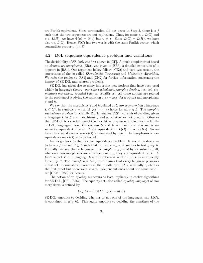
are Parikh equivalent. Since termination did not occur in Step 3, there is a jsuch that the two sequences are not equivalent. Thus, for some u ∈ L(G) andv ∈ L(H), we have Ψ(u) = Ψ(v) but u 6= v. Since L(G) = L(H), we havealso v ∈ L(G). Hence, S(G) has two words with the same Parikh vector, whichcontradicts property (ii). 2

4.2 D0L sequence equivalence problem and variations

The decidability of SE-D0L was first shown in [CF]. A much simpler proof basedon elementary morphisms, [ER2], was given in [ER3], a detailed exposition of itappears in [RS1]. Our argument below follows [CK2] and uses two results, thecorrectness of the so-called Ehrenfeucht Conjecture and Makanin’s Algorithm.We refer the reader to [RS1] and [CK2] for further information concerning thehistory of SE-D0L and related problems.

SE-D0L has given rise to many important new notions that have been usedwidely in language theory: morphic equivalence, morphic forcing, test set, ele-mentary morphism, bounded balance, equality set. All these notions are relatedto the problem of studying the equation g(x) = h(x) for a word x and morphismsg and h.

We say that the morphisms g and h defined on Σ are equivalent on a languageL ⊆ Σ∗, in symbols g ≡L h, iff g(x) = h(x) holds for all x ∈ L. The morphicequivalence problem for a family L of languages, [CS1], consists of deciding, givena language L in L and morphisms g and h, whether or not g ≡L h. Observethat SE-D0L is a special case of the morphic equivalence problem for the familyof D0L languages: two D0L systems G and H with morphisms g and h aresequence equivalent iff g and h are equivalent on L(G) (or on L(H)). So wehave the special case where L(G) is generated by one of the morphisms whoseequivalence on L(G) is to be tested.

Let us go back to the morphic equivalence problem. It would be desirableto have a finite set F ⊆ L such that, to test g ≡L h, it suffices to test g ≡F h.Formally, we say that a language L is morphically forced by its subset L1 iff,whenever two morphisms are equivalent on L1, they are equivalent on L. Afinite subset F of a language L is termed a test set for L iff L is morphicallyforced by F . The Ehrenfeucht Conjecture claims that every language possessesa test set. It was shown correct in the middle 80’s. [AL] is usually quoted asthe first proof but there were several independent ones about the same time –see [CK2], [RS3] for details.

The notion of an equality set occurs at least implicitly in earlier algorithmsfor SE-D0L, [CF], [ER3]. The equality set (also called equality language) of twomorphisms is defined by

E(g, h) = {x ∈ Σ∗| g(x) = h(x)}.

SE-D0L amounts to deciding whether or not one of the languages, say L(G),is contained in E(g, h). This again amounts to deciding the emptines of the

34

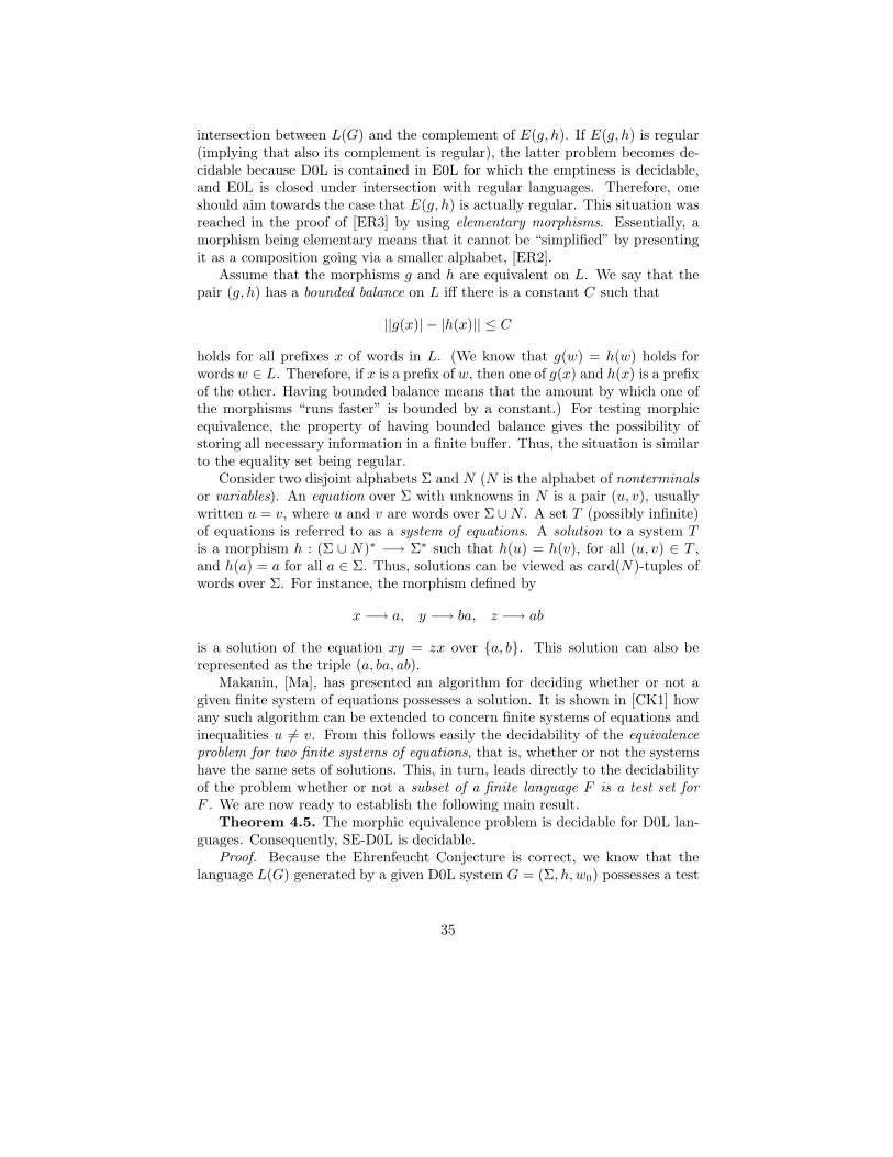
intersection between L(G) and the complement of E(g, h). If E(g, h) is regular(implying that also its complement is regular), the latter problem becomes de-cidable because D0L is contained in E0L for which the emptiness is decidable,and E0L is closed under intersection with regular languages. Therefore, oneshould aim towards the case that E(g, h) is actually regular. This situation wasreached in the proof of [ER3] by using elementary morphisms. Essentially, amorphism being elementary means that it cannot be “simplified” by presentingit as a composition going via a smaller alphabet, [ER2].

Assume that the morphisms g and h are equivalent on L. We say that thepair (g, h) has a bounded balance on L iff there is a constant C such that

||g(x)| − |h(x)|| ≤ C

holds for all prefixes x of words in L. (We know that g(w) = h(w) holds forwords w ∈ L. Therefore, if x is a prefix of w, then one of g(x) and h(x) is a prefixof the other. Having bounded balance means that the amount by which one ofthe morphisms “runs faster” is bounded by a constant.) For testing morphicequivalence, the property of having bounded balance gives the possibility ofstoring all necessary information in a finite buffer. Thus, the situation is similarto the equality set being regular.

Consider two disjoint alphabets Σ and N (N is the alphabet of nonterminalsor variables). An equation over Σ with unknowns in N is a pair (u, v), usuallywritten u = v, where u and v are words over Σ ∪N . A set T (possibly infinite)of equations is referred to as a system of equations. A solution to a system Tis a morphism h : (Σ ∪ N)∗ −→ Σ∗ such that h(u) = h(v), for all (u, v) ∈ T ,and h(a) = a for all a ∈ Σ. Thus, solutions can be viewed as card(N)-tuples ofwords over Σ. For instance, the morphism defined by

x −→ a, y −→ ba, z −→ ab

is a solution of the equation xy = zx over {a, b}. This solution can also berepresented as the triple (a, ba, ab).

Makanin, [Ma], has presented an algorithm for deciding whether or not agiven finite system of equations possesses a solution. It is shown in [CK1] howany such algorithm can be extended to concern finite systems of equations andinequalities u 6= v. From this follows easily the decidability of the equivalenceproblem for two finite systems of equations, that is, whether or not the systemshave the same sets of solutions. This, in turn, leads directly to the decidabilityof the problem whether or not a subset of a finite language F is a test set forF . We are now ready to establish the following main result.

Theorem 4.5. The morphic equivalence problem is decidable for D0L lan-guages. Consequently, SE-D0L is decidable.

Proof. Because the Ehrenfeucht Conjecture is correct, we know that thelanguage L(G) generated by a given D0L system G = (Σ, h, w0) possesses a test

35

set F . We only have to find F effectively. Define the finite languages Li, i ≥ 0,by

L0 = {w0}, Li+1 = Li ∪ h(Li).

We now determine an integer i0 such that Li0 is a test set for Li0+1. Such aninteger surely exists because eventually the whole F is contained in some Li.The integer i0 can be found because we can decide whether a subset of a finitelanguage is a test set. We claim that Li0 is a test set for L(G), which completesthe proof. Indeed, since Li0 is a test set for Li0+1, also Li0+1 \ {w0} is a testset for Li0+2 \ {w}. (Obviously, whenever F ′ is a test set for L′, then h(F ′) isa test set for h(L′).) Consequently, Li0+1 is a test set for Li0+2. Since “being atest set for” is obviously transitive, we conclude that Li0 is a test set for Li0+2,from which our claim follows inductively. 2

If the alphabet consists of two letters, it suffices to test the first four wordsin the given D0L sequences in order to decide sequence equivalence. This resultis optimal, as shown by the example

w0 = ab, g(a) = abbaabb, g(b) = a, h(a) = abb, h(b) = aabba.

This has given rise to the 2n-conjecture: in order to decide SE-D0L, it sufficesto test the first 2n words in the sequences, where n is the cardinality of thealphabet. No counterexamples to this conjecture have been found, although theonly known bound of this kind is really huge, [ER4].

Theorems 4.4 and 4.5 yield immediatelyTheorem 4.6. LE-D0L is decidable.We are able to establish now also the following very strong result.Theorem 4.7. The HD0L sequence equivalence problem is decidable.Proof. Without loss of generality, we assume that the two given HD0L

systems are defined by the morphisms f1 and f2 and D0L systems H = (Σ, h, w0)and G = (Σ, g, w0), respectively. We consider a “barred copy” Σ of the alphabetΣ: Σ = {a| a ∈ Σ}. The “barred version” w of a word w ∈ Σ∗ is obtainedby barring each letter. We define three new morphisms, using the descriptivenotations f1, f2 and h ∪ g, as follows:

f1(a) = f1(a), f2(a) = λ, (h ∪ g)(a) = h(a) for a ∈ Σ,

f1(a) = λ, f2(a) = f2(a), (h ∪ g)(a) = g(a) for a ∈ Σ.

Clearly, the original HD0L sequences are equivalent iff the morphisms f1 and f2

are equivalent on the D0L language defined by the morphism h ∪ g and axiomw0w0. Thus, Theorem 4.7 follows by Theorem 4.5. 2

The decidability of the HD0L sequence equivalence is a very nontrivial gen-eralization of the decidability of SE-D0L. For instance, no techniques based onbounded balance can be used because two morphisms may be equivalent on aD0L language L without having bounded balance on L. Our simple argumentfor Theorems 4.5 and 4.7 is no miraculous “deus ex machina”. Two very strong

36

tools (Ehrenfeucht and Makanin) have been used. (We want to mention in thisconnection that, in spite of their efforts, the editors failed in including in thisHandbook a reasonably detailed exposition of Makanin’s theory.) For a class-room proof, where all tools are developed from the beginning, the proof basedon elementary morphisms, presented in [RS1] or [S5], is still to be recommended.

Some related results are collected in our last theorem. See also [CK2], [Ru2],[Ru3], [Ru4].

Theorem 4.8. The morphic equivalence is decidable for HDT0L languages,and so is the equivalence between D0L and F0L and between D0L and DT0L,as well as the inclusion problem for D0L. The equivalence is undecidable forDT0L, and so is the PD1L sequence equivalence. 2

5 L Growth

5.1 Communication and commutativity

This section will discuss growth functions associated to sequences generated byL systems. The theory will be presented in an unconventional way, as a dis-cussion between a mathematician, a language theorist and a wise layman. Wehave two reasons for this unconventional approach. First, there already existgood detailed expositions of the theory in a book form, [SS], [RS1]. In a conven-tional exposition, we could not do much better here than just repeat, even in acondensed form, what has been already said in [SS] or [RS1]. Secondly, growthfunctions require considerably more factual knowledge in mathematics than doother parts of the L system theory. Since L systems in general are of inter-est to a wide audience not otherwise working with mathematics, conventionalmathematical formulation might scare away many of the readers of this chapter.While we are convinced that this is less likely to happen with our expositionbelow, we also hope that our presentation will open new perspectives also for amathematically initiated reader.

Dramatis personae

Bolgani, a formal language theorist,Emmy, a pure mathematician,Tarzan, a lonesome traveller.

Emmy. I often wonder why we mathematicians always write texts incom-prehensible practically to everybody. Of course every science has its own ter-minology and idioms, but our pages laden with ugly-looking formulas are stilldifferent. I have the feeling that in many cases the same message could beconveyed much more efficiently using less Chinese-resembling text.

Bolgani. Just think how Fermat got his message across, in a passage thathas influenced the development of modern mathematics perhaps more than anypassage of comparable length. Cubum autem in duos cubos, aut quadratoquadra-

37

tum in duos quadratoquadratos, et generaliter nullam in infinitum ultra quadra-tum potestatem in duos ejusdem nominis fas est dividere: cujus rei demonstra-tionem mirabilem sane detexi. Hanc marginis exiguitas non caperet1. Isn’t itlike beautiful poetry? And think of the philosophical implications. That some-thing is correct is expressed by saying “fas est” – follows the divine law. Noteven the gods among themselves can break mathematical laws.

Emmy. It still remains a problem whether some “demonstratio mirabilis”exists for Fermat’s Last Theorem. One can hardly imagine that Fermat had inmind anything even remotely resembling the fancy methods of Andrew Wiles.But coming back to poetry: the words sound beautiful but one has to knowsomething in order to appreciate the beauty.

Tarzan. Some basic knowledge is always necessary but in many cases ratherlittle will suffice. Take a passage from Horace, also with references to divineactivities.Pone me pigris ubi nulla campis arbor aestiva recreatur aura, quodlatus mundi nebulae malusque Juppiter urget. Pone sub curru nimium propinquisolis, in terra domibus negata: dulce ridentem Lalagen amabo, dulce loquentem2.Certainly it sings much better than Fermat. But still you have to have somebackground in order to fully appreciate it, a mere understanding of the languageis not enough.

Bolgani. I have an idea. Tarzan already read about the basics of L systems.(This refers to Sections 1 and 2 above.) Let us try to explain to him the theoryof growth functions, using as few formulas as possible. This might open someinteresting perspectives, even if no poetry would come up.

Tarzan. I already know something about the topic. Take, for instance, aD0L system. It generates a sequence of words. One considers the length of eachword, as a function of the position of the word in the sequence. This functionwill be the growth function of our D0L system. One starts counting the positionsfrom 0, the axiom having the position 0. This means that every growth functionmaps the set of nonnegative integers into the same set. Some things are obvioushere. The growth function of a PD0L system is monotonously increasing, notnecessarily strictly increasing at every step, whereas decrease is possible in theD0L case. Whenever 0 appears as a value of a D0L growth function, thenall values afterwards, that is values for greater arguments, are also equal to 0.Whenever we have the empty word in the sequence, then only the empty wordappears afterwards. Once dead, always dead. No resurrection is possible in thismodel of life, be it real or artificial. However, this is the only restriction I have.

1“It is improper (by divine right) to divide a cube into two cubes, a fourth power intotwo fourth powers and, generally, any power beyond a square into two powers with the sameexponent as the original. I really found a miraculous proof for this fact. However, the marginis too small to contain it.”

2“Place me where never summer breeze/ Unbinds the glebe, or warms the trees/ Whereever-lowering clouds appear,/ And angry Jove deforms th’inclement year:// Place me beneaththe burning ray,/ Where rolls the rapid car of day;/ Love and the nymph shall charm mytoils,/ The nymph, who sweetly speaks and sweetly smiles.” (Ode XXII, tr. by P.FrancisHorace, Vol.I, London, printed by A.J.Valpy, M.A., 1831)

38

If I can take as many letters as I want, I can get the first million, billion orany number of values exactly as I like: 351, 17, 1934, 1, 1964, 15, 5, 1942,... Ijust introduce new letters at every step, getting the lengths as I like. Since myalphabet is altogether finite, at some stage there will be repetitions of lettersand, accordingly, patterns in the growth sequence. The over-all growth cannotbe more than exponential. The length of the ith word is bounded from aboveby ci+1, where the constant c equals the maximum of the lengths of the axiomand any right-hand side of the rules. This bound is valid for DIL systems aswell.

Bolgani. We are dealing here with issues concerning communication andcommutativity. I think we have already agreed that we can communicate witheach other in a less formal manner – even about technically complicated topics.Commutativity is the key to D0L growth functions. It also opens the possibilityof using strong mathematical tools. Why do we have commutativity? Becausethe order of letters is completely irrelevant from the point of view of growth.We only have to keep track of the number of occurrences of each letter or, as thesaying goes, of the Parikh vector of the word. Only the number is significant,we can commute the letters as we like. But we have to know the Parikh vector,it is not sufficient to know the total length of the word. Two different lettersmay grow very differently.

Emmy. All information we need can be stored in the growth matrix ofthe D0L system. It is a square matrix, with nonnegative integer entries anddimension equal to the cardinality of the alphabet, say n. We have a fixedordering of the letters in mind, and the rows and columns of the matrix areassociated to the letters according to this ordering. The third entry in thesecond row indicates how many times the third letter occurs on the right side ofthe rule for the second letter. In this way the matrix gives all the informationwe need for studying growth.

Take our old friend SQUARES as an example. The rules were a −→ abc2,b −→ bc2, c −→ c. The growth matrix is, accordingly,

1 1 20 1 20 0 1

See that? The first entry in the second row is 0, because there are no a’s onthe right side of the rule for b. To complete the information, we still need theParikh vector of the axiom. In this case it is Π = (1, 0, 0) since the axiom is a.

So far we have been able to store the information in matrix form. We nowcome to the point which makes the play with matrices really worthwhile. Onederivation step amounts to multiplication by the growth matrix if we are onlyinterested in the length sequence. This is a direct consequence of the rule formatrix multiplication. Let us go back to SQUARES and take the word abc2bc4 inthe sequence, two steps after the axiom. Its Parikh vector is (1, 2, 6). Compute

39

the matrix product (1, 2, 6)M . It is another Parikh vector, obtained as follows.You take a column of M , multiply its entries by the corresponding entry of(1, 2, 6), and sum up the products. If your chosen column is the first one, thisgives the result 1 · 1+ 2 · 0+ 6 · 0 = 1, and 1 · 1+ 2 · 1+ 6 · 0 = 3 and 1 · 2+2 ·2+ 6 ·1 = 12 in the other two cases. Altogether we get the new Parikh vector(1, 3, 12). What does, for instance, the last entry tell us? The third column

221

indicates how many c’s each of the letters a, b, c produces. The numbers ofoccurrences of the letters were 1, 2, 6 to start with. Thus, the last entry 12 =1 · 2+ 2 · 2+ 6 · 1 tells how many c’s we have after an additional derivation step.Similarly the entries 1 and 3 tell how many a’s and b’s we have.

There is nothing in our conclusion pertaining to the particular exampleSQUARES. We have shown that after i derivation steps we have the Parikhvector Π M i. (This holds true also for i = 0.) Let η be the n-dimensionalcolumn vector with all components equal to 1. The values f(i) of the growthfunction are obtained by summing up the components of the Parikh vectorΠ M i,

f(i) = Π M i η, i ≥ 0.

We have derived the basic interconnection with the theory of matrices, and havenow all the classical results available, [MT], [HW].

Tarzan. I know some of them. For instance, the Cayley-Hamilton Theoremsays that every matrix satisfies its own characteristic equation. If we have nletters in the alphabet, we can express Mn in terms of the smaller powers:

Mn = c1Mn−1 + . . . + cn−1M

1 + cnM0,

in this case with integer constants cj . By the matrix representation for thegrowth function, we can use the same formula to express each growth functionvalue in terms of values for smaller arguments:

f(i + n) = c1f(i + n − 1) + . . . + cnf(i), i ≥ 0.

I see it now quite clearly. I can do my arbitrary tricks at the beginning. Butonce the number of steps reaches the size of the alphabet, I am stuck with thisrecursion formula.

Bolgani. We will see that many mysteries remain in spite of the formula.But the formula surely gives rise to certain regularities. For instance, the so-called “Lemma of Long Constant Intervals”. Assume that f is a D0L growthfunction and, for every k, there is an i such that

f(i) = f(i + 1) = . . . = f(i + k).

40

Then f is ultimately constant: there is an i0 such that f(i) = f(i0) for all i ≥ i0.The matrix representation gives also a very simple method for deciding

growth equivalence: two D0L systems G and G′, with alphabet cardinalitiesn and n′, possess the same growth function iff the lengths of the first n + n′

terms are the same in both sequences. The bound is the best possibe. Thisalgorithm is very simple, both as regards the proof of its validity and as re-gards the resulting procedure. This striking contrast to the difficulty of theD0L sequence equivalence problem is again due to commutativity. Consider anexample of language-theoretic interest. Two D0L systems have both the axioma. The rules of the first system are a −→ ab3, b −→ b3, and the rules of thesecond system:

a −→ acde, b −→ cde, c −→ b2d2, d −→ d3, e −→ bd.

You can verify that the first seven numbers in both length sequences are 1, 4,13, 40, 121, 364, 1093. Hence, the systems are growth equivalent.

Tarzan. The D0L system DEATHb had the axiom ab2a and the rules a −→ab2a, b −→ λ. We noticed that cell death is necessary to generate its language.However, the very simple system with the axiom a4 and rule a −→ a2 is growthequivalent, and is without cell death. What is really the role of cell death, thatis rules a −→ λ, in D0L growth? Does it consist only of making decreasespossible? What is the difference between D0L and PD0L growth? If I have anon-decreasing D0L growth function, can I always get the same function usinga PD0L system, perhaps at the cost of taking vastly many new letters?

Emmy. That would be too good to be true. The effects of cell death aredeeper, also from the growth point of view. The answer to your question is“no”, and we still come to the difference between D0L and PD0L growth. Atthe moment, I would like to dwell on more immediate matters.

The interconnection with matrices, in particular the recurssion formula youare stuck with, open the possibility of using a lot of classical results from thetheory of matrices and difference equations. The values f(i) can be expressedas “exponential polynomials” in i, that is, finite sums of terms of the form

(α0 + α1i + . . . + αt−1it−1)ρi.

Indeed, here ρ is a root, with multiplicity t, of the characteristic equation of M .Maybe you like an example. Take the system with the axiom abc and the rules

a −→ a2, b −→ a5b, c −→ b3c,

yielding

M =

2 0 05 1 00 3 1

41

Since the matrix is in lower diagonal form, the roots of the characteristic equa-tion are seen immediately: 2 and 1 (double). This results in the expression

f(i) = (α0 + α1i) · 1i + α2 · 2

i

for the growth function. Finally, the coefficients α are determined by consideringthe first few values (here first three) in the length sequence. Observe that herethe axiom becomes important – so far we did not use it at all! The final resultis

f(i) = 21 · 2i − 12i − 18.

This solves the growth analysis problem for any system: we can write downthe exponential polynomial representing the growth function of the system.Although the values f(i) are nonnegative integers, the numbers ρ and α arecomplex numbers, sometimes not even expressible by radicals. Since the growthfunction is always an exponential polynomial, some growth types can never oc-cur as D0L growth. D0L growth cannot be logarithmic: whenever the growthfunction is not bounded by a constant, the growth is at least linear. Similarly,nothing faster than exponential or between polynomially bounded and expo-nential, something like the 2

√n, is possible.

Bolgani. Such in-between growth orders are possible in the DIL case, [K1].As Tarzan already observed, super-exponential growth is impossible also in theDIL case.

Emmy. Still a few things. The theory says a lot also about the converseproblem, growth synthesis. We have in mind a function, obtained experimentallyor otherwise, and we want to construct a D0L system having the function asits growth function. For instance, we can synthesize any polynomial p(i) withinteger coefficients and assuming integer values for all integers i ≥ 0. (p(i)may assume negative values for non-integral values of i.) We cannot synthesizei2 − 4i + 4 because it represents death at i = 2, but i2 − 41 + 5 is OK. It is thegrowth function of the D0L system with the axiom a3

1a2a3 and rules

a1 −→ λ, a2 −→ a4, a3 −→ a5, a4 −→ a6, a5 −→ λ,

a6 −→ ad, a −→ abc2, b −→ bc2, c −→ c, d −→ d.

Observe that our old friend SQUARES is lurking in the stomach of this newD0L creature, where Tarzan’s technique of disposable letters is also visible.

Making use of periodicities, we can also synthesize several polynomials in asingle D0L system. Explicitly, this technique of merging means the following.Assume that we have some synthesizable polynomials, say p0(i), p1(i), p2(i), ofthe same degree. Then we can construct a D0L system whose growth functionsatisfies, for all i,

f(3i) = p0(i), f(3i + 1) = p1(i), f(3i + 2) = p2(i).

42

It is essential that the polynomials are of the same degree; in general, the quo-tient of two mergeable functions should be bounded from above by a constant.

Recall the matrix representation of D0L growth functions, f(i) = Π M i η.Functions of this form, where M is a square matrix and Π and η are row andcolumn vectors of the same dimension, all with integer entries, are termedZ-rational. (This terminology is quite natural, see [SS].) If the entries arenonnegative integers, the function is termed N-rational. D0L growth functionsare a special case of N-rational functions: it is required that all entries in ρ areequal to 1. PD0L growth functions are a further special case: it is also requiredthat every row of M has a positive entry. The part of the matrix theory thatcomes into use here is customarily referred to as the Perron-Frobenius theory.

5.2 Merging and stages of death

Bolgani. We now face the challenging task of discussing the differences betweenthe four classes of functions Emmy just introduced. By definition, the classesconstitute an increasing hierarchy from PD0L growth functions (smallest class)to Z-rational functions (biggest class). That the inclusions between the classesare strict is also obvious. N-rational functions cannot assume negative values,as Z-rational functions clearly can. 0, 1, 1,... is an N-rational but not a D0Llength sequence. Decrease is possible in D0L but not in PD0L length sequences.Such examples can be viewed as trivial, forced by definitions. However, in eachcase we can show the strictness of the inclusion also by a nontrivial example.Moreover, mathematically very nice characterizations are known for each of thefour classes of functions. Emmy should say more about it, let me just give thefollowing rough idea.

The difference between Z-rational and N-rational functions stems from theidea of merging or mergeability. An N-rational sequence can always be obtainedby merging sequences with a “clean dominant term”, whereas this is not nec-essarily possible for Z-rational sequences. By a “clean dominant term” I meanthat the expression for an individual member of the sequence has a term αikρi,where α, ρ are constants and k is a nonnegative integer, completely determiningthe growth, that is, the member is asymptotically equal to this term. One cansay that the growth order of the term, as a function of its position i, equals ikρi.As you recall, ρ is a root of the characteristic equation and can in general be acomplex number but is real in a clean dominant term.

The difference between D0L and PD0L growth functions can be said tohappen at the primary stage of death: death affected by the rewriting modelitself. We will see that mathematically this difference amounts again to thedifference between Z-rational and N-rational functions. Finally, the differencebetween N-rational and D0L comes from the fact that a secondary stage of deathis possible for the former. Because some entries of the final vector ρ may equal0, letters can be erased after the actual D0L sequence has been created. Wecan also speak of death occurring in the system, contrasted with death caused

43

by outside forces.Tarzan. I can see the difference between N-rational and D0L very clearly.

The secondary stage of death can be viewed also as the invisibility of someletters: the letters themselves cannot be seen, although they sometimes producevisible offsprings. Take the very simple D0L system with the axiom ac and rules

a −→ b, b −→ a, c −→ d2, d −→ c.

Take

η =

1001

so only a and d are kept visible. See? In the underlying D0L sequence a andb alternate, similarly c and d, and the latter also affect exponential growth.But because of death caused by outside forces, the exponential growth is visibleonly at even stages, the length sequence being 1, 2, 1, 4, 1, 8, ... . This isobtained by merging a constant and an exponential sequence. Only sequenceswith the same growth order can be merged in a D0L system. This follows

because clearly f(i+1)f(i) is bounded from above by a constant, an obvious choice

being the maximal length of the right sides of the rules. It is clear by definitionthat N-rational functions coincide with HD0L growth functions. It is also easyto prove directly that if all entries of η are positive then the N-rational functionis, in fact, a D0L growth function: a D0L system can be constructed by useof a dummy “filling letter” that takes care of the components of η exceeding 1.This means that the secondary stage of death, caused by the entries 0 in η, isreally the essential characteristic of N-rational functions, when contrasted withD0L growth functions. The secondary stage of death can be used to eliminatethe primary stage, HPD0L growth functions are the same as HD0L ones. Thisshould be easy enough to establish directly; it is of course also a consequence ofthe characterization result, Theorem 2.3.

Emmy. Essentially everything has already been said. I still want to elabo-rate the fundamental issues. Take first the role of N-rational functions amongZ-rational ones; what Bolgani talked about clean dominant terms. As we haveseen, an individual member of a Z-rational sequence can be expressed as an ex-ponential polynomial. Such an exponential polynomial has a part determiningits growth order: in the asymptotic behavior only this part is significant. Thispart is determined by terms itρi, where ρ has the greatest possible modulus andt is the greatest (for this modulus). Thus, among the roots of the characteris-tic equation of the growth matrix, we are interested in those with the greatestmodulus. There may be many of them since in general the ρ’s are complexnumbers.

Tarzan. What Bolgani spoke about clean dominant terms means of coursethat in the decomposition, in the parts to be merged, the dominant terms are

44

real numbers, implying that the original ρ’s are real numbers multiplied by rootsof unity. This is equivalent to saying that some integral power of ρ is real. Ihave seen that the term rational in degrees is used for such ρ’s: the argumentof ρ is a rational multiple of π – now the classical π, not your initial vector!

Emmy. You have seen many things during your trips, also from our fields.It was shown in [Be] that the phenomenon described by you happens for ρ’s inthe N-rational case, the converse result being due to [So2]. Parts of this theorygo back to Kronecker. What would be an example? Here it is good that youknow some classical analysis. Consider a number α such that

cos 2πα = 3/5, sin 2πα = 4/5.

Then α must be irrational: the imaginary part of (3 + 4i)t is always congruentto 4 modulo 5. Thus, we have here irrationality in degrees. Along these linesone can show that, for instance, the function assuming positive values, definedby

f(2m) = 30m, f(2m + 1) = 25mcos2 2πmα

is Z-rational but not N-rational. It is an interesting detail that Z-rational andN-rational functions coincide in the polynomially bounded case, [SS].

The difference between Z-rational and N-rational functions turns out to bedecisive also in the characterization of PD0L growth functions among D0Lgrowth functions, [So1]. For any D0L growth function f(m), the differencesd(m) = f(m+1)− f(m) constitute a Z-rational function. The function f(m) isa PD0L growth function iff the differences d(m) constitute an N-rational func-tion. (We exclude here the empty word as the axiom.) This result gives thepossibility of using any Z-rational function g(m) assuming nonnegative valuesand being not N-rational to obtain a non-decreasing D0L growth function thatis not a PD0L growth function. The idea is to merge the sequences Rm andRm + g(m), where R is a large enough integer. If you do not like the cosinepresent in the preceding example, I will give you another, still closely relatedexample:

f(2m) = 10m, f(2m + 1) = 10m + m · 5m + (3 + 4i)m + (3 − 4i)m.

Thus, although the total size of this D0L creature keeps increasing all the time, itmust have cells which die immediately! This holds independently of the numberof cell types (letters) we are using.

Bolgani. The D0L system of this example has an estimated 200 letters.You are not likely to find such examples just by playing around with D0Lsystems. The method works here in a backward manner. You begin with someroots ρ, algebraic numbers not rational in degrees. You then construct yourcharacteristic equation, and then the matrix. When you have expressed theresulting Z-rational sequence as the difference of two PD0L sequences, you startto be in business and can work with L systems from that point on. These new

45

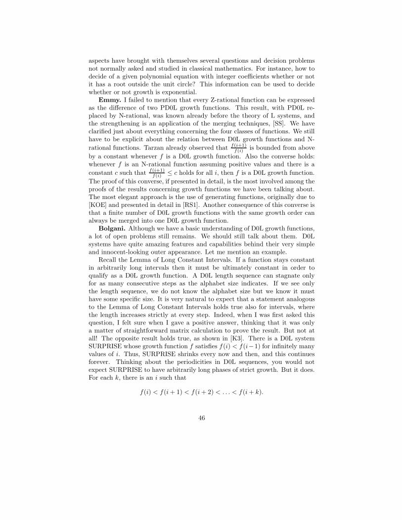
aspects have brought with themselves several questions and decision problemsnot normally asked and studied in classical mathematics. For instance, how todecide of a given polynomial equation with integer coefficients whether or notit has a root outside the unit circle? This information can be used to decidewhether or not growth is exponential.

Emmy. I failed to mention that every Z-rational function can be expressedas the difference of two PD0L growth functions. This result, with PD0L re-placed by N-rational, was known already before the theory of L systems, andthe strengthening is an application of the merging techniques, [SS]. We haveclarified just about everything concerning the four classes of functions. We stillhave to be explicit about the relation between D0L growth functions and N-

rational functions. Tarzan already observed that f(i+1)f(i) is bounded from above

by a constant whenever f is a D0L growth function. Also the converse holds:whenever f is an N-rational function assuming positive values and there is a

constant c such that f(i+1)f(i) ≤ c holds for all i, then f is a D0L growth function.

The proof of this converse, if presented in detail, is the most involved among theproofs of the results concerning growth functions we have been talking about.The most elegant approach is the use of generating functions, originally due to[KOE] and presented in detail in [RS1]. Another consequence of this converse isthat a finite number of D0L growth functions with the same growth order canalways be merged into one D0L growth function.

Bolgani. Although we have a basic understanding of D0L growth functions,a lot of open problems still remains. We should still talk about them. D0Lsystems have quite amazing features and capabilities behind their very simpleand innocent-looking outer appearance. Let me mention an example.

Recall the Lemma of Long Constant Intervals. If a function stays constantin arbitrarily long intervals then it must be ultimately constant in order toqualify as a D0L growth function. A D0L length sequence can stagnate onlyfor as many consecutive steps as the alphabet size indicates. If we see onlythe length sequence, we do not know the alphabet size but we know it musthave some specific size. It is very natural to expect that a statement analogousto the Lemma of Long Constant Intervals holds true also for intervals, wherethe length increases strictly at every step. Indeed, when I was first asked thisquestion, I felt sure when I gave a positive answer, thinking that it was onlya matter of straightforward matrix calculation to prove the result. But not atall! The opposite result holds true, as shown in [K3]. There is a D0L systemSURPRISE whose growth function f satisfies f(i) < f(i−1) for infinitely manyvalues of i. Thus, SURPRISE shrinks every now and then, and this continuesforever. Thinking about the periodicities in D0L sequences, you would notexpect SURPRISE to have arbitrarily long phases of strict growth. But it does.For each k, there is an i such that

f(i) < f(i + 1) < f(i + 2) < . . . < f(i + k).

46

No matter how long a phase you need for SURPRISE to become bigger andstronger during the whole phase, a proper timing gives you such a phase!

5.3 Stagnation and malignancy

Tarzan. Cancer is sometimes identified with exponential growth. I would liketo call growth in a D0L system malignant if, for some rational t > 1 and i0 ≥ 0,

f(i) > ti whenever i ≥ i0.

We know that, for D0L growth functions but not in the DIL case, this is equiv-alent to saying that there is no polynomial p such that f(i) ≤ p(i) holds for alli.

Suppose I want to play a doctor for creatures of artificial life, modeled byD0L systems. One of them comes to me and I have to tell whether or not he/shewill eventually grow cancer. How can I do it? I know how he/she looked as aninfant (the axiom) and the rules for the cell development. It is clear to me that ifthere is some letter that derives in some number of steps two copies of itself andpossibly some other letters as well, then the growth is malignant. Here I takeinto account only letters actually occurring in the sequence, a condition that canbe easily tested. So the occurrence of such an expanding letter is sufficient formalignancy but is it also necessary? Could the creature develop cancer withouthaving any expanding cell? Probably not. If the condition is also necessary andif I can test of any letter whether or not it is expanding, then I can diagnose allcreatures and tell each of them either good or bad news!

Bolgani. You sure can. The necessity of your condition is fairly easy toestablish by purely language-theoretic means. If there are no expanding letters,a growth-equivalent system can be constructed having letters a1, . . . , an suchthat the right side of the rule for ai has at most one ai and no letters aj withj < i. The growth in this new system is bounded by a polynomial of degreen − 1. The system SQUARES is of this type with n = 3. In the early years ofL systems D0L systems of this type were referred to as systems with “rank”.Essentially, the rank r is equivalent with polynomial growth of degree r − 1.

How to test whether a given letter a is expanding? The following algorithmworks. Studying the rules, form a sequence of sets S0, S1, S2, . . . Each set Si willbe a subset of a finite set T , consisting of all letters of the given D0L system, aswell as of all unordered pairs of letters, pairs (b, b) being included. Explicitly,S0 consists of the pair (a, a). For all i, Si+1 is the union of Si and S′

i, where S′i

is obtained as follows. Take an element y of Si. If y is a single letter c appearingon the right side of the rule for b, include b to S′

i. Assume next that y is a pair(b, c). Then we include the letter d to S′

i if both b and c (or b twice if b = c)occur on the right side of the rule for d. Finally, we include the pair (d, e) to S′

i

if the right sides of the rules for d and e, put together, contain both b and c.The sets Si form an increasing sequence of subsets of a finite set T . There

must be an index j such that Sj+1 = Sj . The letter a is expanding exactly in

47

case it belongs to Sj . Indeed, we begin in S0 with the situation where two a’soccur, and investigate backwards all possibilities where they might have comefrom. In Sj we have reached the point where there are no more possibilities.Since Sj+1 = Sj , nothing new can come up later. So it is decisive whether wehave reached a single a latest by Sj. Whenever we reach a single a, we stop.This is bad news for our creature. If we reach Sj without seeing a single a, it isnot yet good news. Every other letter has to be tested in the same way.

Tarzan. In the system DEATHb, a is already in S1, so it is immediatelybad news. If you diagnose b in FIB, you get both (a, a) and (a, b) in S1 and,hence, you get b in S2. The letter a is also expanding but you have to go up toS4 to reach bad news. As you described D0L systems with rank, it seems thatfor them no diagnosis is needed: it follows by the very definition that the systemhas no expanding letters. I can immediately tell the good news to SQUARES.

Emmy. The diagnosis can also be based on powers of the growth matrix,[K2]. You compute powers M i, i = 1, 2, . . .. Whenever you find a diagonalelement greater than 1, you diagnose malignancy. If you have reached the valuei = 2n +n− 1, where n is the dimension, and have found only 0’s and 1’s in themain diagonal, you may tell the good news.

Tarzan. Recall our friends DAY-PAL and NIGHT-PAL. The growth matrixof the former has the diagonal entry 2, corresponding to the letter b. The letterb is reachable from any nonempty axiom, in fact all letters eventually becomeb’s. Thus, it is bad news for any DAY-PAL(w).

I would like to talk about another notion. Bolgani used the term “stagna-tion” in connection with the Lemma of Long Constant Intervals. Let us saythat a D0L sequence stagnates if it has two words wt and wt+p, p > 0, with thesame Parikh vector. Clearly, this implies that

f(i) = f(i + p) for all i ≥ t,

that is, the lengths start repeating periodically with the period p after thethreshold t. The condition is certainly decidable. For instance, we decidewhether the language is finite. Every NIGHT-PAL(w) stagnates. Any axiombecomes a power of c in two steps.

What about a much weaker requirement? A D0L sequence stagnates momen-tarily if f(t) = f(t+1) holds for some t. I can decide momentary stagnation forPD0L sequences. I just look at the subalphabet Σ′ consisting of letters mappedto a letter by the morphism. Momentary stagnation is equivalent to the factthat some subset of Σ′ appears in the sequence of minimal alphabets. Sincethe latter sequence is ultimately periodic, I can decide the fact. But things aredifferent in the general D0L case, and momentary stagnation can take place inmany ways. It sure must be decidable but how can I decide it?

Bolgani. You got me. This happens to be a celebrated open problem. Givena D0L growth function f , one has to decide whether or not f(t) = f(t + 1)holds for some t. The term “constant level” had also been used, instead of

48

your “momentary stagnation”. The following formulation is equivalent in thesense that an algorithm for either one of the problems can be converted into analgorithm for the other problem. Given two PD0L growth functions f and g,decide whether or not f(t) = g(t) holds for some t. An algorithm is known inboth cases, [SS], if “for some t” is replaced by “for infinitely many values of t”.

Emmy. Also the following is an equivalent formulation for the problem ofmomentary stagnation. Given a square matrix M with integer entries, decidewhether or not the number 0 appears in the upper right-hand corner of somepower of M . So far all attempts to determine an upper bound for the exponentsto be tested have failed. The problem is decidable for 2× 2 matrices. Examplesare known of 3×3 matrices where you have to go to the exponent 50 to find thefirst 0. Again, this problem is decidable if you ask for infinitely many 0s insteadof just one 0.

Bolgani. The following problems of proper thinness and continuing growthare more involved than the problem of momentary stagnation, in the sensethat an algorithm for either one of them yields an algorithm for the problemof momentary stagnation but not necessarily vice versa, [PaS], [KS]. Decidewhether or not a given D0L language has two words of the same length. (Alanguage is called properly thin if all its words are of different lengths. This is aspecial case of slenderness.) Decide whether or not a given D0L growth functionf satisfies the inequality f(i) ≤ f(i + 1) for all i.

Tarzan. The whole theory of growth functions can apparently be extendedto concern DT0L systems as well. Take the system PAL, with some specificaxiom. Once we have fixed an order of the tables Tn and Td, that is a wordover the alphabet {n, d}, we end up with a unique word. From the growth pointof view we get a mapping f of the set of words over the alphabet of tables, inthe example {n, d}, into the set of nonnegative integers. In the D0L case thealphabet of tables consists of one letter only. In the DT0L case we can askbasically the same questions as before. Growth equivalence makes sense onlyif the table alphabets are of the same cardinality. Momentary stagnation takesplace if there is a word x and letter a such that f(xa) = f(x). We are nowdealing with several growth matrices, one for each letter of the table alphabet;Mn and Md for PAL. We get the expression ΠMdMnMdMnρ for the lengthof the DAY-AND-NIGHT-PAL after 48 hours – you understand what I mean.One can also start with a fixed DT0L system, for instance PAL, and investigatewhat kind of growth phenomena are possible or likely to happen.

Emmy. One can also introduce Z-rational and N-rational functions as be-fore, now the domain of the functions will be some Σ∗ instead of N . Fromthe point of view of power series, [SS], [KS], this means several noncommutingvariables. Several undecidability results are obtained by a reduction to Hilbert’sTenth Problem, for instance, the undecidability of the problems of momentarystagnation and continuing growth. On the other hand, growth equivalence canbe shown decidable by a nice argument using linear spaces, [RS1].

Tarzan. It seems to me that you can be proud of many nice and certainly

49

nontrivial results. Many challenging problems remain open. After some progressin areas such as artificial life you surely will ask entirely new kinds of questionsabout L growth. I have to go.

6 L codes, number systems, immigration

6.1 Morphisms applied in the way of a fugue

In the remainder of this chapter, we will present some recent work dealing withL systems. Two problem areas will be presented in more detail in Sections 6and 7, whereas the final Section 8 will run through results in different areas ina rather telegraphic way. Unavoidably, the choice of material reflects at leastto some extent our personal tastes. However, we have tried to choose materialsignificant beyond L systems, as well as to present techniques showing the powerof language-theoretic methods in completely different areas, a typical examplebeing the results concerning number systems presented below.

The purpose of this Section 6 is to present some recent work in L systems,dealing with several developmental processes that have started at different times.One can visualize the different processes as chasing one another like the tunesin a fugue. We will restrict our attention to D0L processes. In fact, apartfrom some suggestions, very little work concerning other types of L systemshas been done in this problem area, although most questions can be readilygeneralized to concern also other types of L systems. The issues discussedbelow will concern also generalized number systems, combinatoricss on words,codes and cryptography.

We consider again morphisms h : Σ∗ −→ Σ∗. The morphisms can be usedas an encoding in the natural way: words w over Σ are encoded as h(w). If h isinjective, decoding will always be unique. This is not the case for the morphismh defined by

h(a) = ab , h(b) = ba, h(c) = a.

The word aba can be decoded both as ac and cb because h is not injective.Because of unique decodability, injective morphisms are referred to as codes.There is a chapter below in this Handbook dealing with the theory of codes.Usually codes are defined as sets of words rather than morphisms. For finitecodes, our definition is equivalent to the customary definition in the followingsense. A morphism h is a code iff the set {h(a)| a ∈ Σ} is a code, provided h isnon-identifying, that is, a 6= b implies h(a) 6= h(b) for all letters a and b. We stillrepeat the decodability aspect in terms of cryptography. The morphism h beinga code means that every “cryptotext” w′ can be “decrypted” in at most oneway, that is, there is at most one “plaintext” w that is “encrypted” by h into w′:h(w) = w′. Most “monoalphabetic” cryptosystems in classical cryptography arecodes in this sense.

50

We now come back to the morphism h : Σ∗ −→ Σ∗ (not necessarily injective)and apply it in the “fugue way”. This means that h is applied to the first letter,h2 to the second, h3 to the third, and so on, the results being catenated. Thisgives rise to a mapping h : Σ∗ −→ Σ∗, referred to as the L associate of h. Wenow give the formal definition.

Definition. Given a morphism h : Σ∗ −→ Σ∗, its L associate h is definedto be the mapping of Σ∗ into Σ∗ such that always

h(a1a2 . . . an) = h(a1)h2(a2) . . . hn(an),

where the a’s are (not necessarily distinct) letters of Σ. By definition, h(λ) = λ.The morphism h is termed an L code iff its L associate is injective, that is, thereare no distinct words w1 and w2 such that h(w1) = h(w2). 2

The L associate h is rather seldom a morphism itself. In fact, h is a morphismexactly in case h is idempotent, that is, h2 = h. Also the equation hh =hh is not valid in general, which makes many problems concerning L codesrather involved. Consider the classical “Caesar cipher” h affecting a circularpermutation of the English alphabet:

h(a) = b, h(b) = c, . . . , h(y) = z, h(z) = a.

For the L associate we obtain, for instance,

h(aaaa) = bcde, h(dcba) = eeee.

The L associate is not a morphism but h is both a code and an L code, satisfyingthe equation hh = hh. The proof of the next result is straightforward.

Theorem 6.1. Every code is an L code but not vice versa. 2

A significant class of L codes that are not codes results by considering unarymorphisms. By definition, a morphism h is unary iff there is a specific let-ter a such that h(b) is a power of a for every letter b. (Unary morphismsshould not be confused with unary L systems; for the former, the alphabet Σmay still contain several letters.) Consider the unary morphism h defined by(*) h(a) = a2, h(b) = a.Clearly, h is not a code, for instance, h(bb) = h(a). However, h is an L code.Indeed, this follows by considering dyadic representations of integers, with thedigits 1 and 2. Compute the exponents of a in h(aaa), h(baaba), h(bbbb):

2 ·20+2 ·21+2 ·22, 1 ·20+2 ·21+2 ·22+1 ·23+2 ·24, 1 ·20+1 ·21+1 ·22+1 ·23.

Observe that the original letters b and a behave exactly as the digits 1 and2, respectively, in the dyadic representation of positive integers. For instance,baaba represents the number 53, written in dyadic notation 21221 = 2 · 24 + 1 ·23 + 2 · 22 + 2 · 21 + 1 · 20.

See [S1] for an exposition concerning n-adic and n-ary number systems. Inboth cases n is the base of the representation, but the digits are 1, 2, ...,n in

51

the n-adic and 0, 1,..., n − 1 in the n-ary representation; 1, 2 in dyadic, and0,1 in binary representation. The presence of 0 among the digits renders n-arysystems ambiguous, because an arbitrary number of initial 0’s can be added toany word without changing the represented number. n-adic representation isunambiguous. There is a one-to-one correspondence between positive integersand nonempty words over {1, 2} when the latter are viewed as dyadic represen-tations. Normally in number systems the leftmost digit is defined to be the mostsignificant one, and we will follow this practice below. The definition of an Lassociate, which is the natural one because words are normally read from left toright, makes the rightmost letter most significant because there the morphismis iterated most. Thus, actually the mirror image 12212 of the dyadic word21221 corresponds to the original word baaba. This technical inconvenience (ofgoing from words to their mirror images) is irrelevant as regards ambiguity. Themorphism h defined by (*) is an L code. If there were two distinct words w andw′ such that h(w) = h(w′), then the mirror images of w and w′ would be (inter-preting b as the digit 1 and a as the digit 2) two distinct dyadic representationsfor the same number, which is impossible.

Similarly, one can associate a number system to any unary morphism. Themorphism is an L code iff the number system is unambiguous. This quiteremarkable interconnection between number systems and L systems will now bepresented more formally.

Definition. A number system is a (v + 1)-tuple

N = (n, m1, . . . , mv)

of positive integers such that v ≥ 1, n ≥ 2, and 1 ≤ m1 < m2 < . . . < mv. Thenumber n is referred to as the base and the numbers mi as digits. A nonemptyword mik

mik−1. . .mi1mi0 , 1 ≤ ij ≤ v over the alphabet {m1, . . . , mv} is said

to represent the integer

[mik. . . mi0 ] = mi0 + mi1n + mi2n

2 + . . . + miknk.

The set of all represented integers is denoted by S(N). A set of positive integersis said to be representable by a number system (briefly, RNS), if it equals theset S(N) for some number system N . Two number systems N1 and N2 arecalled equivalent if S(N1) = S(N2). A number system N is called complete ifS(N) equals the set of all positive integers, and almost complete if there areonly finitely many positive integers not belonging to S(N). A number system istermed ambiguous if there are two distinct words w1 and w2 over the alphabet{m1, . . . , mv} such that [w1] = [w2]. Otherwise, N is termed unambiguous.An RNS set is termed unambiguous if it equals S(N), for some unambiguousnumber system N . Otherwise, it is termed inherently ambiguous.2

Number systems as defined above are often referred to as “generalized num-ber systems”. They are more general than the customary notion because thenumber and size of the digits is independent of the base. Some integers may

52

also have several representations or none at all. On the other hand, we haveexcluded the digit 0 (ordinary binary and decimal systems do not qualify) be-cause it immediately induces ambiguity. For each n ≥ 2, the number systemN = (n, 1, 2, . . . , n) is complete and unambiguous. It is customarily referred toas the n-adic number system.

Let h : Σ∗ −→ Σ∗ be a unary morphism. Thus, there is a letter a ∈ Σ suchthat all h-values are powers of a. Assume that h(a) = an, n ≥ 2. The associatednumber system is defined by

N(h) = (n, m1, . . . , mv),

where the mi’s are the exponents, arranged in increasing order, in the equationsh(b) = ami where b ranges over the letters of Σ. (We assume that h is non-erasing and non-identifying. The assumptions about h are needed to ensure thatN(h) is indeed a number system. On the other hand, if h(a) = a or h is erasingor identifying, it is not an L code.) Observe that the base is always among thedigits in a number system N(h). By the above discussion, the following theoremis an immediate consequence of the definitions.

Theorem 6.2. A unary morphism is an L code iff the associated numbersystem is unambiguous. 2

L codes were introduced in [MSW2], where also the basic interconnectionswith number systems were discussed. The ambiguity problem for number sys-tems was shown decidable in [Ho1]. The theory of generalized number systemswas initiated in [CS2]. We focus here our attention to basic issues and issuesconnected with L codes. The reader is referred to [Ho2] – [Ho9] for relatedproblems and some quite sophisticated results (concerning, for instance, regu-larity, degrees of ambiguity, changes of the base and negative digits). The nexttheorem summarizes some basic results from [MSW2] and [CS2].

Theorem 6.3. A number system N = (n, m1, . . . , mv) is ambiguous ifv > n. N is unambiguous if the digits mj lie in different residue classes modulon. No finite set is RNS, whereas every cofinite set is RNS, Every union ofsome residue classes modulo n, n ≥ 2, is RNS. Consequently, both even andodd numbers form RNS sets. The former is unambiguous, whereas the latteris inherently ambiguous. There is an RNS set possessing representations withdifferent bases m and n such that it has an unambiguous representation withm, whereas every representation with the base n is ambiguous. There are a 0Lsystems G and a DT0L system G1, both with the alphabet {a, b} such that

L(G) = L(G1) = {b} ∪ {bai| i ∈ S(N)}.2

Equivalence is undecidable for 0L systems, whereas it is decidable for U0L sys-tems (see Theorems 4.2 and 4.3). The last sentence of Theorem 6.3 gives asomewhat stronger decidability result. This follows by the decidability resultsfor number systems, discussed still in Section 6.2.

53

Is an arbitrary given morphism an L code? At the time of this writing,the decidability of this problem is open in its general form, There is everyreason to believe the problem to be decidable, especially because the remainingclass of morphisms with an open decidability status seems rather small. Forunary morphisms, the decidability follows by Theorem 6.2. The decidabilitywas established for permutation-free morphisms in [Ho4], that is, for morphismsh such that h permutes no subalphabet Σ1 of Σ. The next theorem gives thedecidability result in its strongest known form, [Ho7].

Given a morphism h : Σ∗ −→ Σ∗, we call a letter a bounded (with respect toh) if there is a constant k such that |hn(a)| ≤ k holds for all n. Otherwise, a issaid to be growing. A letter a is pumping if hn(a) = uav holds for some n andwords u and v such that uv is nonempty but contains only bounded letters.

Theorem 6.4. It is decidable whether or not a morphism for which noletter is pumping is an L code. 2

6.2 An excursion into number systems

This subsection deals exclusively with number systems. We feel that such abrief excursion is appropriate to show the versatility of L systems. The workdealing with L codes has led to problems dealing with the representation ofpositive integers in arbitrary number systems. Typical questions concern theequivalence and ambiguity of number systems. In spite of their fundamentalnumber-theoretic nature and also in spite of the fact that the representationof integers is fundamental in the theory of computing, very little was knownabout the solution of such problems before the interconnection with L codeswas discovered. Many of the results below are interesting also withing a generallanguage-theoretic setup: no other than a language-theoretic proof is knownfor these number-theoretic results. Our exposition will be illustrated by someexamples.

Consider first the number system N1 = (2, 2, 3, 4). We claim that S(N1)consists of all positive integers that are not of the form 2k − 3, for some k ≥ 2.(Thus, 1, 5, 13, 29, 61 are the first few numbers missed.) To show that nonumber of this form is in S(N1) we proceed indirectly. Let x = 2k − 3 be thesmallest such number in S(N1), and consider the representation [a1 . . . am] = x.We must have m ≥ 2 and am = 3 because, otherwise, the represented number iseven. But now obviously [a1 . . . am−1] = 2k−1 −3, contradicting the choice of x.On the other hand, for any k ≥ 1, an arbitrary integer x satisfying 2k+1−2 ≤ x ≤2k+2 − 4 is represented by some word of length k, the upper and lower boundsbeing represented by 2k and 4k, respectively. Thus, our claim concerning S(N1)follows. The system N1 is ambiguous: [32] = [24] = 8. The first sentence ofTheorem 6.3 can be used to show that S(N1) is inherently ambiguous. In thedyadic number system (2, 1, 2), S(N1) is represented by all words over {1, 2}that are not of the form 2i1, for some i ≥ 0. (Thus, a regular expression canbe given for the set of words representing S(N1) in dyadic notation. A general

54

statement of this fact is contained in the Translation Lemma below.)The number system N2 = (2, 1, 4) is unambiguous, by the second sentence of

Theorem 6.3. We claim that S(N2) equals the set of numbers incongruent to 2modulo 3. Indeed, all numbers in S(N2) are of this type. This is clearly true ofnumbers represented by words of length 1 over the digit alphabet. Whenever x iscongruent to 0 (resp.1) modulo 3, then both 2x+1 and 2x+4 are congruent to 1(resp.0) modulo 3. Hence, by induction, every number in S(N2) is incongruentto 2 modulo 3. That all such numbers are in S(N2) is again seen indirectly.If x = 3k or x = 3k + 1 is the smallest such number outside S(N2), we canconstruct by a simple case analysis a still smaller number outside S(N2).

Very simple number systems can lead to tricky situations not yet clearlyunderstood. Consider, for k ≥ 3, the number system N(k) = (2, 2, k). Whenis N(k) unambiguous? This happens if k is odd or if k = 2m with an evenm. The remaining case is not so clear. The first odd values of m yielding anunambiguous N(K) are: 11, 19, 23, 27, 35, 37, 39, 43, 45, 47, 51, 53, 55, 59,67, 69, 71, 75, 77, 79, 83, 87, 89, 91, 93, 95, 99. [MSW2] contains a morecomprehensive theory about this example.

We now introduce a tool basic for decidability results. It consists of viewingthe sets S(N) as regular languages.

Translation Lemma. Given a number system N = (n, m1, . . . , mv), a reg-ular expression α(N) over the alphabet {1, . . . , n} can be effectively constructedsuch that the set of words in the regular language denoted by α(N), when thewords are viewed as n-adic numbers, equals S(N). 2

The reader is referred to [CS2] for details of the proof. The argument is avery typical one about regular languages and finite automata. It is easy to geta rough idea. A finite automaton (sequential machine) translates words w#,where w ∈ {m1, . . . , mv}+, into words over {1, . . . , n}. The word w is viewedas a number represented according to N in reverse notation, and the translatewill be the representation of the same number in reverse n-adic notation. The“carry” (due to digits exceeding the base) is remembered by the state of theautomaton. (A reader not familiar with this terminology is referred to Chapter2 of this Handbook.) It turns out that 2 max(n, mv) states will suffice. In onestep, when reading the letter j in the state i, the automaton outputs j′ andgoes to the state i′, where i′ and j′ are unique integers satisfying

i + j = j′ + i′n, 1 ≤ j′ ≤ n.

When reading the boundary marker # in the state i, the automaton producesthe output i in reverse n-adic notation. This is the only step, where the outputmay consist of more than one letter.

As an example, consider the number system N = (2, 13, 22). We use thenotation a = 13, b = 22 to avoid confusion. The computation of the automatonfor the input abaa# looks as follows:

55

state 0 6 13 12 12input a b a a #output 1 2 2 1 212new state 6 13 12 12

The mirror image aaba of the input abaa represents in N the number 213:

[aaba] = 13 · 23 + 13 · 22 + 22 · 2 + 13 = 213.

The mirror image 2121221 of the output is the dyadic representation of 213. Wehave already pointed out the notational inconvenience caused by the fact thatin the number-system notation the leftmost digit is the most significant one.

The claims in the following theorem are either immediate consequences ofthe Translation Lemma, or can be inferred from it using decidability resultsconcerning regular languages.

Theorem 6.5. It is decidable whether or not a given number system isambiguous, complete or almost complete. The equivalence problem is decidablefor number systems. It is undecidable whether or not a given recursively enu-merable set is RNS. It is also undecidable, given a recursively enumerable set Sand an integer n ≥ 2, whether or not there is a number system N with base nsuch that S = S(N). It is decidable of a given number system N and an integern ≥ 2 whether or not there exists an unambiguous number system N ′ with basen satisying S(N) = S(N ′). 2

For the number system N = (3, 1, 3, 4, 6, 7) and n = 2, the decision methodof the last sentence produces the number system N ′ = N2 = (2, 1, 4) alreadydiscussed above. On the other hand, every representation of S(N) with base 3is ambiguous. Thus, although the property characterizing S(N) is intimatelyconnected with the number 3, one has to choose a different base in order to getan unambiguous representation of S(N)!

Using more sophisticated methods, dealing with recognizable sets and formalpower series, the decidability of the equivalence can be extended to concernnumber systems with arbitrary integer digits, [Ho5]. Also the final theorem inthis subsection, [Ho9], results from an application of such methods. A weakerversion of the theorem was established in [Ho6].

Theorem 6.6. Given a number system, it is decidable whether or not thereexists an equivalent unambiguous number system. 2

6.3 Bounded delay and immigration

We now return to codes and L codes. For easier reference, we use certain boldletters to denote classes of morphisms: C stands for the class of codes and L forthe class of L codes. The notation P refers to prefix codes, that is, morphisms hfor which there are no distinct letters a and b for which h(a) is a prefix of h(b).(It is clear that morphisms satisfying this condition are codes.) We now presentthe idea of bounded delay.

56

With cryptographic connotations in mind, let us refer to the argument was plaintext and to the encoded version h(w) or h(w) as cryptotext. The ideabehind the bounded delay is the following. We do not have to read the wholecryptotext on order to start writing the plaintext but rather always a certainprefix of the cryptotext determines the beginning of the plaintext.

The notation prefk(w) for the prefix of w of length k ≥ 1 was already in-troduced in Section 2. The notation first(w) stands for the first letter of anonempty word w. A morphism h is of bounded delay k if, for all words u andw, the equation

prefk(h(u)) = prefk(h(w))

implies the equation first(u) = first(w). The morphism h is of bounded delay,in the class B, if it is of bounded delay k, for some k. It is again easy to seethat the property of bounded delay implies the property of being a code. Themorphism h defined by

h(a) = aa, h(b) = ba, h(c) = b

is a code but not of bounded delay. Indeed, one might have to read the wholecryptotext in order to determine whether the first plaintext letter is b or c.Different notions of bounded delay are compared in [Br] and [BeP]. The sameclass B is obtained no matter which definition is chosen, but different definitionsmay lead to different minimal values of k.

The idea of bounded delay is the same for codes and L codes: first k lettersof the cryptotext determine the first plaintext letter. For codes the situationremains unaltered after handling the first letter a, because the cryptotext is stillof the form h(w) when h(a) has been removed from the beginning. However, forL codes, the remainder of the cryptotext equals hh(w) rather than h(w). Thismeans that we obtain different notions of bounded delay, depending on whetherwe are interested in finding only the first plaintext letter (weak notion, W), orthe first letter at each stage of decryption (strong or medium strong notion).The difference between the two latter notions depends on the way of boundingthe delay: is the bound kept constant (strong notion S), or is it allowed to growaccording to the stage of decryption (medium strong notion, M). We now givethe formal definition.

Definition. A morphism h is of weakly bounded delay k ≥ 1 if, for all wordsu and w, the equation

prefk(h(u)) = prefk(h(w))

implies the equation first(u) = first(w). If for all i ≥ 0 and all u and w, theequation

prefk(hih(u)) = prefk(hih(w))

implies the equation first(u) = first(w), then h is of strongly bounded delay k.In general, h is of weakly or strongly bounded delay if it is so for some k. The

57

notations W and S are used for the corresponding classes of morphisms. Finally,h is of medium bounded delay (notation M) if, for some recursive function f andall i ≥ 0, u and w, the equation

preff(i)(hih(u)) = preff(i)(h

ih(w))

implies the equation first(u) = first(w). 2

Observe that we do not require h to be an L code in these definitions. Thesituation is analogous to that concerning ordinary codes. However, a morphismbeing in B implies that it is in C, whereas L and W are incomparable. Allinclusion relations between the classes introduced are presented in the followingtheorem [MSW3].

Theorem 6.7. The mutual inclusion relations between the families intro-duced are given by the following diagram, where an arrow denotes strict inclu-sion and two families are incomparable if they are not connected by a path:

C LS P B

M W

2

Medium bounded delay can be viewed in the theory of L codes as the mostnatural counterpart of bounded delay codes. It is natural to require that only abounded amount of lookahead at each stage of the decryption process is needed.If the amount of lookahead remains the same throughout the process, the re-sulting notion is a very restricted one, as will be seen below. On the otherhand, the drawback in the definition of M is that, in general, the constructionof the sequence of values f(i) = ki, i = 0, 1, 2, . . ., seems to be an infinitarytask. The following theorem, [HoS], is pleasing because it shows that it sufficesto construct values only up to card(Σ) − 2.

We say that a morphism h : Σ∗ −→ Σ∗ is an the set M’ if, for some k > 0and all i with 0 ≤ i ≤ card(Σ) − 2, the equation

prefk(hih(u)) = prefk(hih(w))

always implies the equation first(u) = first(w). Thus, we consider the sequencef(i) = ki only up to card(Σ) − 2, and take the maximum of the resultingnumbers.

Theorem 6.8. M’ = M. 2

We now present a simple characterization for the family S.Theorem 6.9. A morphism h is in S iff, for any distinct letters a and b,

first(h(a)) 6= first(h(b)).Proof. Consider the “if”-part. The assumption means that there is a per-

mutation Π of the alphabet Σ such that, for all a,

first(h(a)) = Π(a).

58

Consequently, for all i ≥ 0 and a,

first(hi(a)) = Πi(a).

Therefore,pref1(h

ih(a)) = first(hi+1(a)) = Πi+1(a)

uniquely determines a, that is, h is of strongly bounded delay 1.For the “only if” part, we need two auxiliary results that are simple exercises

concerning morphisms. Growing letters were defined at the end of Subsection6.1.

Claim 1. Assume that h is a code and a is a letter. Then either a is growing,or else |hi(a)| = 1, for all i.

Claim 2. If h is a prefix code and a is growing, then first(h(a)) is growing.Let h be in S. By Theorem 6.7, h is a prefix code. We proceed indirectly

and assume that there are two distinct letters a and b such that first(h(a)) =first(h(b)). Since h is a prefix code, we may write

h(a) = cxdy and h(b) = cxez,

where x, y, z are (possibly empty) words and c, d, e are letters such that d 6= e.By Claim 1, a and b are growing. By Claim 2, also c is growing. Hence, forevery k, there is an i such that

prefk(hih(a)) = prefk(hi+1(a)) = prefk(hi+1(b)),

which contradicts the assumption that h is in S. 2

At the time of this writing, no general decision method is known for testingmembership in M or W.

Some more sophisticated decidability results are obtained, [Ho7], by consid-ering ambiguity sets closely connected with the theory of L codes. Essentially,a morphism being an L code means that the ambiguity set is empty. It can beshown that in most cases the ambiguity set is regular, which leads to decidabil-ity.

Variations in degrees of iteration constitutes the basic idea behind L codes.One can view the definition also as developmental processes started at differenttimes. The same idea has led to the notion of L systems with immigration.One begins with a finite set of words consisting, intuitively, of “beginnings”,“origins”, “atoms”, “founding fathers” that start to develop in an environment.An L system is used to model the development in the environment. The moretime has elapsed since immigration, the more steps have been taken in thedevelopmental process.

For any types of L systems, the corresponding system with immigration canbe defined. However, so far only D0L systems have been investigated in thisrespect. We conclude with a few remarks about this area. We begin with adefinition.

59

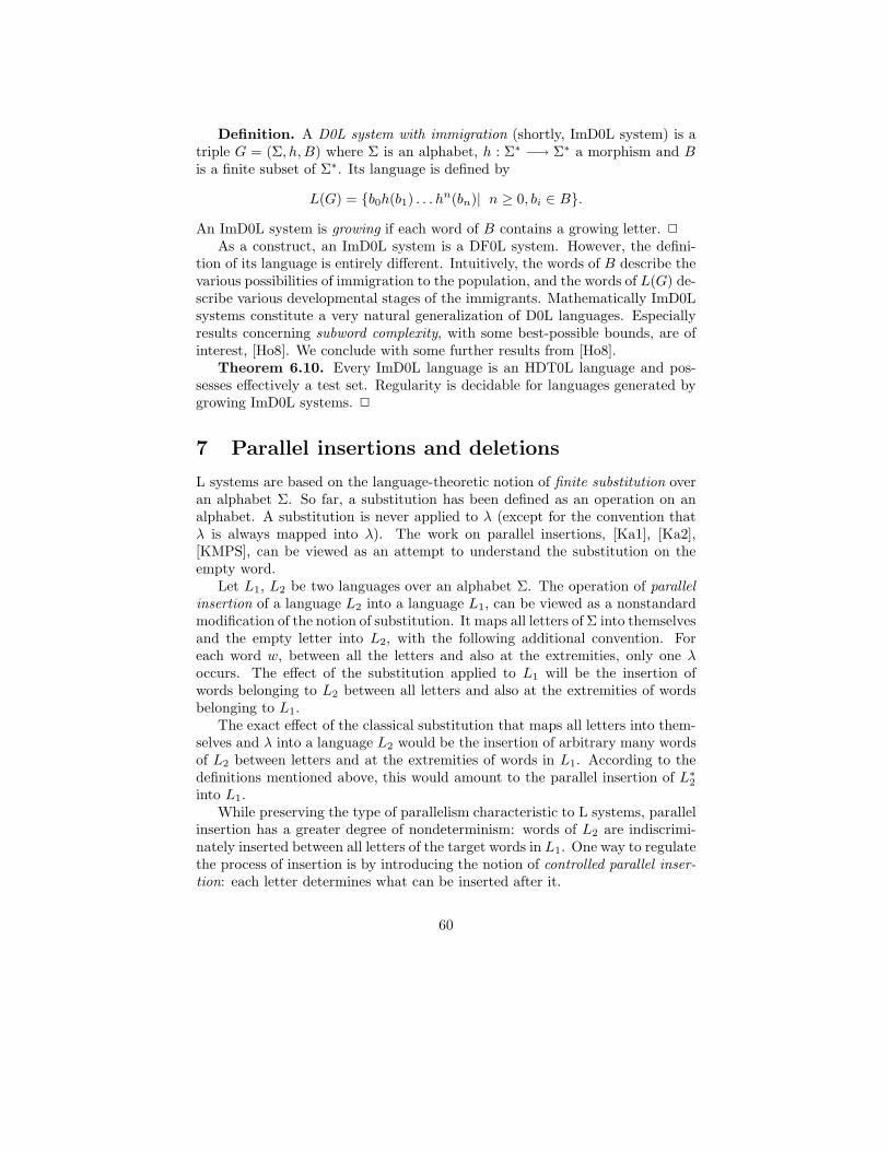
Definition. A D0L system with immigration (shortly, ImD0L system) is atriple G = (Σ, h, B) where Σ is an alphabet, h : Σ∗ −→ Σ∗ a morphism and Bis a finite subset of Σ∗. Its language is defined by

L(G) = {b0h(b1) . . . hn(bn)| n ≥ 0, bi ∈ B}.

An ImD0L system is growing if each word of B contains a growing letter. 2

As a construct, an ImD0L system is a DF0L system. However, the defini-tion of its language is entirely different. Intuitively, the words of B describe thevarious possibilities of immigration to the population, and the words of L(G) de-scribe various developmental stages of the immigrants. Mathematically ImD0Lsystems constitute a very natural generalization of D0L languages. Especiallyresults concerning subword complexity, with some best-possible bounds, are ofinterest, [Ho8]. We conclude with some further results from [Ho8].

Theorem 6.10. Every ImD0L language is an HDT0L language and pos-sesses effectively a test set. Regularity is decidable for languages generated bygrowing ImD0L systems. 2

7 Parallel insertions and deletions

L systems are based on the language-theoretic notion of finite substitution overan alphabet Σ. So far, a substitution has been defined as an operation on analphabet. A substitution is never applied to λ (except for the convention thatλ is always mapped into λ). The work on parallel insertions, [Ka1], [Ka2],[KMPS], can be viewed as an attempt to understand the substitution on theempty word.

Let L1, L2 be two languages over an alphabet Σ. The operation of parallelinsertion of a language L2 into a language L1, can be viewed as a nonstandardmodification of the notion of substitution. It maps all letters of Σ into themselvesand the empty letter into L2, with the following additional convention. Foreach word w, between all the letters and also at the extremities, only one λoccurs. The effect of the substitution applied to L1 will be the insertion ofwords belonging to L2 between all letters and also at the extremities of wordsbelonging to L1.

The exact effect of the classical substitution that maps all letters into them-selves and λ into a language L2 would be the insertion of arbitrary many wordsof L2 between letters and at the extremities of words in L1. According to thedefinitions mentioned above, this would amount to the parallel insertion of L∗

2

into L1.While preserving the type of parallelism characteristic to L systems, parallel

insertion has a greater degree of nondeterminism: words of L2 are indiscrimi-nately inserted between all letters of the target words in L1. One way to regulatethe process of insertion is by introducing the notion of controlled parallel inser-tion: each letter determines what can be inserted after it.

60

Another way to look at operations of controlled insertion is the following.Such an operation can be viewed as a production of the form a −→ aw, wherethe word w comes from the language to be inserted next to a. The mode ofcontrolled insertion determines how the productions are going to be applied.The controlled parallel insertion resembles, thus, the rewriting process of 0Lsystems. However, it gives rise to something different from 0L systems becausethe productions are always of the special form and, on the other hand, there areinfinitely many productions.

Formally, if L1, L2 are languages over the alphabet Σ, the parallel insertionof L2 into L1 is defined as:

L1 ⇐= L2 =⋃

u∈L1

(u ⇐= L2),

where

u ⇐= L2 = {v0a1v1a2v2 . . . akvk| k ≥ 0, aj ∈ Σ, 1 ≤ j ≤ k,

vi ∈ L2, 0 ≤ i ≤ k and u = a1a2 . . . ak}.

The case k = 0 corresponds to the situation u = λ, when only one word v0 ∈ L2

is inserted.As parallel insertion is associative, it induces a monoid structure on P(Σ∗),

the set of all subsets of Σ∗, with {λ} as the neutral element. The monoid isnot commutative. For example, a ⇐= b = {bab} whereas b ⇐= a = {aba}.The families of regular, context-free and context-sensitive languages are closedunder parallel insertion. Indeed, for L1, L2 languages over Σ we have thatL1 ⇐= L2 = L2s(L1), where s is the λ-free substitution defined by

s : Σ∗ −→ 2Σ∗

, s(a) = aL2, for every a ∈ Σ.

The assertion above now follows as the families of regular, context-free andcontext-sensitive languages are closed under catenation and λ–free substitutions.

The parallel insertion amounts thus to the application of a single substitu-tion. If, as in the case of L systems, we consider iterated applications of thesubstitution, the obtained operation is much more powerful than the parallelinsertion: starting with two one-letter words the iterated parallel insertion canproduce a non-context-free language. Formally, if L1, L2 are languages overΣ, the parallel insertion of order n of L2 into L1 is inductively defined by theequations:

L1 ⇐=0 L2 = L1,L1 ⇐=k+1 L2 = (L1 ⇐=i L2) ⇐= L2, i ≥ 0.

The iterated parallel insertion of L2 into L1 is then defined as

L1 ⇐=∗ L2 =

∞⋃

n=0

(L1 ⇐=n L2).

61

The iterated parallel insertion is not commutative: the word bbb belongs toλ ⇐=∗ b but not to b ⇐=∗ λ. It is not associative either as the word cbcabbelongs to a ⇐=∗ (b ⇐=∗ c) but not to (a ⇐=∗ b) ⇐=∗ c.

The iterated parallel insertion of the letter b into itself is

b ⇐=∗ b = {b2k−1| k > 0},

which proves that the families of regular and context-free languages are notclosed under iterated parallel insertion. However, the family of context-sensitivelanguages is still closed under it. Indeed, given two context-sensitive gram-mars G1 and G2 generating the languages L1 and L2, a grammar G generatingL1 ⇐=∗ L2 can be obtained as follows. G contains the rules of G2, the rulesof G1, and the rules of G1 modified in such a way that next to each letter, theaxiom of G2 is attached.

An interesting variation on the theme of parallel insertion is to combine itwith the commutative closure. The commutative closure of a language L is thesmallest commutative language containing L . The commutative closure can beviewed as a unary operation associating to every language L its commutativeclosure com(L). The permuted parallel insertion of the word v into u consiststhus of the parallel insertion into u of all words which are letter-equivalent tov (Two words are letter-equivalent if one of them is obtained by permuting theletters of the other.)

More precisely, L1 ⇐=p L2 =⋃

u∈L1,v∈L2(u ⇐= com(v)). Obviously, the

permuted parallel insertion can be expressed as L1 ⇐=p L2 = L1 ⇐= com(L2).As expected , the fact that the families of regular and context-free languages arenot closed under the commutative closure implies that they are not closed underpermuted parallel insertion. On the other hand, being closed under both parallelinsertion and commutative closure, the family of context-sensitive languages isclosed under permuted parallel insertion.

We have dealt so far with operations where the same language is insertedin parallel between all the letters and at the extremities of a given word. Theprocess resembles more the type of rewriting characteristic to L systems if everyletter determines what can be inserted after it. Let L be a language over Σ and∆ : Σ −→ 2Σ∗

a so-called control function satisfying ∆(a) 6= ∅, ∀a ∈ Σ. The∆–controlled parallel insertion into L (shortly controlled parallel insertion) isdefined as:

L ⇐=c ∆ =⋃

u∈L

(u ⇐=c ∆),

where

u ⇐=c ∆ = {a1v1a2v2 . . . akvk| u = a1 . . . ak, k ≥ 1, ai ∈ Σ.

and vi ∈ ∆(ai), 1 ≤ i ≤ k}.

Note that in the above definition, the control function cannot have the empty setas its value. This condition has been introduced because of the follwing reason.

62

If there would exist a letter a ∈ Σ such that ∆(a) = ∅, then all the words u ∈ Lwhich contain a would give u ⇐=c ∆ = ∅. This means that these words wouldnot contribute to the result of the controlled parallel insertion. Consequentlywe can introduce, without loss of generality, the condition ∆(a) 6= ∅, ∀a ∈ Σ.

If we impose the restriction that for a distinguished letter b ∈ Σ we have∆(b) = L2, L2 ⊆ Σ∗, and ∆(a) = λ for every letter a 6= b, we obtain a particularcase of controlled parallel insertion: parallel insertion next to the letter b. Itis a binary language operation, whereas the arity of the ∆-controlled parallelinsertion equals card(Σ) + 1.

The families of regular, context-free and context-sensitive languages areclosed under controlled parallel insertion. This follows as the result of the con-trolled parallel insertion L ⇐=c ∆, where L ⊆ Σ∗ and ∆ : Σ −→ 2Σ∗

, ∆(a) 6= ∅,∀a ∈ Σ, can be accomplished by the λ-free substitution

σ : Σ∗ −→ 2Σ∗

, σ(a) = a∆(a), ∀a ∈ Σ.

For each of the above mentioned variants of insertion, a dual deletion opera-tion can be defined. Take, for example, the parallel deletion. Given words u andv, the parallel deletion of v from u consists of the words obtained by simultane-ously erasing from u all the nonoverlapping occurrences of v. The definition isextended to languages in the natural way. Given a word u and a language L2,the parallel deletion u =⇒ L2 consists of the words obtained by erasing from uall the nonoverlapping occurrences of words in L2:

u =⇒ L2 = {u1u2 . . . ukuk+1| k ≥ 1, ui ∈ Σ∗, 1 ≤ i ≤ k + 1 and∃vi ∈ L2, 1 ≤ i ≤ k such that u = u1v1 . . . ukvkuk+1,where {ui} ∩ [Σ∗(L2 \ {λ})Σ∗] = ∅, 1 ≤ i ≤ k + 1}.

Note that, besides the fact that the parallel deletion erases from u nonoverlap-ping occurrences of words from L2, a supplementary condition has to be fulfilled:between two occurrences of words of L2 to be erased, no nonempty word fromL2 appears as a subword. This assures that all occurrences of words from L2

have been erased from u, and is taken care of by the last line of the definition.The reason why λ had to be excluded from L2 is clear. If this wouldn’t be thecase and λ would belong to L2, the condition {ui} ∩ Σ∗L2Σ

∗ = ∅ would imply{ui} ∩ Σ∗ = ∅ – a contradiction. Note that words from L2 can still appear assubwords in u =⇒ L2, as the result of catenating the remaining pieces of u. IfL1, L2 are languages over Σ, we can define now L1 =⇒ L2 = ∪u∈L1

(u =⇒ L2).If L, R are languages over the alphabet Σ, L a λ-free language and R a

regular one, then there exists, [Ka1], a rational transducer g, a morphism h anda regular language R′ such that L =⇒ R = h(g(L) ∩ R′). As a corollary, thefamilies of regular and context-free languages are closed under parallel deletionwith regular languages. On the other hand, the family of context-free languagesis not in general closed under parallel deletion. For example, consider Σ = {a, b}

63

and the context-free languages:

L1 = #{aib2i| i > 0}∗,

L2 = #a{biai| i > 0}∗.

If the language L1 =⇒ L2 would be context-free, then also the language

(L1 =⇒ L2) ∩ b+ = {b2n

| n > 0},

would be context-free, which is a contradiction.A similar nonclosure situation happens in the case of context-sensitive lan-

guages: there exists a context-sensitive language L1 and a word w over analphabet Σ such that L1 =⇒ w is not a context-sensitive language. Indeed, letL be a recursively enumerable language (which is not context-sensitive) over analphabet Σ and let a, b be two letters which do not belong to Σ. Then thereexists a context-sensitive language L1 such that (see [S1]):

(i) L1 consists of words of the form aibα, where i ≥ 0 and α ∈ L;(ii) For every α ∈ L, there is an i ≥ 0 such that aibα ∈ L1.It is easy to see that aL1 =⇒ {a} = bL, which is not a context-sensitive

language. We have catenated a to the left of L1 in order to avoid the case i = 0,when the corresponding words from L would have been lost.

In a similar way we have defined the iterated parallel insertion, we candefine the iterated parallel deletion. Despite of the simplicity of the languagesinvolved, it is an open problem whether or not the family of regular languagesis closed under iterated parallel deletion. Not only that, but it is still an openproblem whether the iterated parallel deletion of a singleton word from a regularlanguage still belongs to the family of regular languages. The answer to bothof the previous questions is negative in the case of context-free and context-sensitive languages. For example, if we consider the alphabet Σ = {a, b}, thecontext-free language L = {ai#b2i| i > 0}∗, and the word w = ba then

(L =⇒∗ ba) ∩ a#+b+ = {a#nb2n

| n > 0},

which implies that L =⇒∗ ba cannot be context-free.The permuted parallel deletion of a language L2 from L1 is obtained by

erasing from words in L1 words that are letter-equivalent to words in L2:

L1 =⇒p L2 =⋃

u∈L1,v∈L2

(u =⇒p v),

where u =⇒p v = u =⇒ com(v). If Σ = {a, b} and L1 = $a∗b∗##a∗b∗$ andL2 = #$(ab)∗ then the permuted parallel deletion of L2 from L1 is

L1 =⇒p L2 = {$anbm#| m, n ≥ 0, m 6= n}∪{#anbm$| m, n ≥ 0, m 6= n} ∪ {λ},

64

which shows that the result of permuted parallel deletion between two regularlanguages is not necessarily regular. If L1 is the context-free language

L1 = {an1 bm

1 cl1#cl

2bm2 an

2#| n, m, l ≥ 0}

and L2 is the regular language L2 = ##(a2b2c2)∗ then

L1 =⇒p L2 = {an1 bn

1 cn1 | n ≥ 0}.

This shows that the family of context-free languages is not closed under per-muted parallel deletion with regular languages. By using an argument similarto the one used for parallel deletion, one can show that the family of context-sensitive languages is not closed under permuted parallel deletions with singletonlanguages.

A controlled variant of the parallel deletion can be defined as follows. Letu ∈ Σ∗ be a word and ∆ : Σ −→ 2Σ∗

be a control function which does not have∅ as its value. The set u =⇒c ∆ is obtained by finding all the nonoverlappingoccurrences of ava, va ∈ ∆(a), in u, and by deleting va from them. Betweenany two ocurrences of words of the type ava, va ∈ ∆(a), in u, no other wordsof this type may remain.

If one imposes the restriction that for a distinguished letter b ∈ Σ we have∆(b) = L2, and ∆(a) = λ for any letter a 6= b, a special case of controlledparallel deletion is obtained: parallel deletion next to the letter b. The parallel

deletion next to the letter b is denoted byb

=⇒. Let us examine the set ub

=⇒ L2,where u is a nonempty word and L2 is a language over an alphabet Σ. If u = bk,k > 0, and no word of the form bv, v ∈ L2 occurs as a subword in u, the set

ub

=⇒ L2 equals the empty set. If u contains at least one letter different from b,u is retained in the result as we can erase λ near that letter. The other wordsin u

b=⇒ L2 are obtained by finding all the nonoverlapping occurrences of words

of the type bvi, vi ∈ L2 in u, and deleting vi from them. There may exist morethan one possibility of finding such a decomposition of u into subwords.

One can use similar techniques as for the parallel deletion to show that thefamily of regular languages is closed under controlled parallel deletion, while thefamilies of context-free and context-sensitive languages are not (except when thelanguages to be deleted are regular).

Besides studying closure properties, one can get more insight into the powerof parallel insertion and deletion operations by investigating classes of languagesthat contain simple languages and are closed under some of the operations. Sucha class should be closed under a parallel insertion operation, a parallel deletionone and an iterated parallel insertion one. Particular controlled operations willbe chosen in order to allow an increase as well a decrease of the length of thewords in the operands. The iterative operation has been included to provide aninfinite growth of the strings. Finally, we have to introduce the mirror imageand the union with λ for technical reasons.

65

Thus, let P be the smallest class of languages which contains the empty set,the language {λ}, the singleton letters and is closed under mirror image, unionwith {λ}, controlled parallel insertion, iterated controlled parallel insertion andcontrolled parallel deletion with singletons. Then, [Ka2], P is contained in thefamily of context-sensitive languages and properly contains the family of regularlanguages. If we replace in P the controlled parallel deletion with singletons byunrestricted controlled parallel deletion, the new family P ′ is a Boolean algebraproperly containing the family of regular languages.

The study of parallel insertion and deletion operations is closely connectedto the study of equations involving them. If ⋄ denotes a parallel insertion ordeletion operation, the simplest equations to consider are of the form L⋄X = R,Y ⋄L = R, where R is a regular language, L is an arbitrary language, and X, Yare the unknown languages.

If ⋄ denotes parallel insertion, permuted parallel insertion or parallel in-sertion next to a letter, the problem whether there exists a singleton solutionX = {w} to the equation L ⋄ X = R is decidable for regular languages L andR. Indeed, if ⋄ denotes parallel insertion, let L, R be regular languages andm be the length of the shortest word in R. If there exists a word w such thatL ⇐= w = R then it must satisfy the condition lg(w) ≤ m. As the family of reg-ular languages is closed under parallel insertion, our problem is decidable. Thealgorithm for deciding it will consist of checking whether or not L1 ⇐= w = Rfor all words w with lg(w) ≤ m. The answer is YES if such a word exists andNO otherwise. A similar proof can be used to show that, for ⋄ denoting parallelinsertion, controlled parallel insertion and parallel insertion next to a letter, theexistence of a singleton solution Y to the equation Y ⋄ L = R is decidable forregular languages L and R.

In contrast, given context-free languages L and regular languages R, theexistence of both a solution and a singleton solution X , to the equation L⋄X =R is undecidable for ⋄ denoting parallel insertion, iterated parallel insertion,permuted parallel insertion or parallel insertion next to a letter. Let # be aletter which does not belong to Σ. We can actually prove a stronger statement:there exists a fixed regular language R = Σ∗# such that the problem aboveis undecidable for context-free languages L1. This follows by noticing that theequation (L1#) ⇐= X = Σ∗# holds for languages L1, X over Σ exactly incase L1 = Σ∗ and X = λ. Hence, if we could decide our problem, we wouldbe deciding the problem “Is L1 = Σ∗?” for context-free languages L1, whichis impossible. A similar proof, taking R = Σ∗ ∪ {#} and L1 = L ∪ {#}, canbe used to show that the existence of both a solution and singleton solution Yto the equation Y ⇐= L = R is undecidable for context-free languages L andregular languages R. Analogously it can be shown that the existence of both asolution and singleton solution to the equation Y ⇐= ∆ = R is undecidable forcontext-free control functions and regular languages R.

If we consider the same problems for parallel deletion operations, specialattention has to be paid to the fact that, while the result of parallel insertion is

66

always a word or set of words, the result of parallel deletion can be the emptyset. If ⋄ denotes a binary deletion operation and L is a given language, a wordy is called right-useful with respect to L and ⋄ if there exists x ∈ L such thatx ⋄ y 6= ∅. A language X is called right-useful with respect to L and ⋄ if itconsists only of right-useful words with respect to L and ⋄. The notion of leftuseful can be similarly defined.

In the following, when we state the undecidability of the existence of asolution to a certain equation, we will mean in fact that the existence of a usefulsolution is undecidable. For example, if ⋄ denotes the parallel deletion, permutedparallel deletion or iterated parallel deletion, the existence of a solution to theequation L ⋄ X = R is undecidable for context-free languages L and regularlanguages R. Let us consider the case of parallel deletion. If $, # are lettersthat do not occur in Σ, there exists a regular language R = #Σ+# ∪ $Σ∗$such that our problem is undecidable for context-free languages L. Indeed, fora context-free language L, consider the language L1 = #Σ+# ∪ $L$. For alllanguages L2 ⊆ Σ∗, the equation

#Σ+# ∪ $L$ =⇒ X = #Σ+# ∪ $Σ∗$

holds if and only if X = {λ} and L = Σ∗. If we could decide our problem, wecould decide whether for given context-free languages L, the equation L = Σ∗

holds, which is impossible.The problem remains undecidable even if instead of considering a binary

operation, like parallel deletion, we consider a card(Σ)+1 – ary operation likecontrollel parallel deletion. It can be namely shown that the existence of asingleton control function with the property L =⇒c ∆ = R is undecidable forcontext-free languages L and regular languages R. The proof is similar to thepreceding one and is based on the fact that the equation

L1$ ∪ {#a$| a ∈ Σ} =⇒c ∆ = Σ+ ∪ {#a| a ∈ Σ}

holds for L1 ⊆ Σ∗ and singleton control functions ∆ if and only if

∆(#) = ∆($) = λ, ∆(a) = $, a ∈ Σ and L1 = Σ+.

The operations of parallel insertion and deletion are associated with severalnotions rather basic in the combinatorics of words. A parallel deletion set is aset of the form w =⇒ L, w ∈ Σ∗, L ⊆ Σ∗. Parallel deletions sets are universalin the sense that every finite language can be viewed as a parallel deletion set(see [KMPS]). If we fix the nonempty finite set F in the equation

w =⇒ L = F,

we can ask for an algorithm deciding for a given context-free language L whetheror not a solution w to the equation w =⇒ L = F exists. If such an algorithmexists, we say that F is CF-decidable, otherwise CF-undecidable. F is called

67

CF-universal if for any (nonempty) context-free language L, there is a word wsuch that w =⇒ L = F . We have that the set {λ} is CF-universal and it is theonly CF-universal set.

In spite of the fact that parallel deletion sets coincide with finite sets, everyfinite nonempty set F 6= ∅ is CF-undecidable, ([KMPS]).

The parallel deletion number, [KMPS], associated to a word w equals thecardinality of the largest parallel deletion set arising from w, that is

pd(w) = max{card(w =⇒ L)| L ⊆ Σ∗}.

For the alphabet with only one element, pd(w) can be computed, but for thegeneral case the question seems not to be simple at all. Indeed, one can showthat if w = an, n ≥ 1, then pd(w) = n. In the case of arbitrary alphabets withat least two symbols the following surprising result, [KMPS], is obtained. Ifcard(Σ) ≥ 2, then there is no polynomial f such that for every w ∈ Σ∗ we havepd(w) ≤ f(|w|).

Let us prove this result. It suffices to show that, given a polynomial f (inone variable), there are strings w such that pd(w) > f(|w|).

Take a polynomial f of degree n ≥ 1 and consider the strings

wn,m = (ambm)n.

Moreover, takeLm = {aibj | 1 ≤ i, j ≤ m − 1}.

and evaluate the cardinality of wn,m =⇒ Lm.As each string in Lm contains at least one occurrence of a and one occurrence

of b, we can delete from wn,m exactly n strings of Lm, which implies

wn,m =⇒ Lm = {am−i1bm−j1am−i2bm−j2 . . . am−inbm−jn |

1 ≤ is, js ≤ m − 1, 1 ≤ s ≤ n}.

Consequently,card(wn,m =⇒ Lm) = (m − 1)2n.

Clearly, because 2n is a constant, for large enough m we have

pd(wn,m) ≥ (m − 1)2n > f(2nm) = f(|wn,m|),

which completes the proof.We observed that, for every word w, w =⇒ Σ∗ = {λ}. We can express

this by saying that every word collapses to the empty word when subjected toparallel deletion with respect to Σ∗. We speak also of the collapse set of Σ∗.Thus, the collapse set of Σ∗ equals Σ∗. In general, we define the collapse set ofa nonempty language L ⊆ Σ∗ by

cs(L) = {w ∈ Σ∗| w =⇒ L = {λ}}.

68

This language is always nonempty because it contains each of the shortest wordsin L. For example, cs({anbn| n ≥ 1}) = (ab)+ and cs({a, bb}) = a∗bb(a+bb)∗a∗∪a+, hence cs(L) can be infinite for finite L. On the other hand, cs({ab} ∪{anbmap| n, m, p ≥ 1}) = {ab}, hence cs(L) can be finite for infinite L. Wehave that, [KMPS], there is a linear language L such that cs(L) is not context-free. Indeed, take

L = {ddanbmcn| n, m ≥ 1} ∪ {danbmcp| n, m, p ≥ 1, m ≥ p}.

While it is clear that L is linear,

cs(L) ∩ d2a+b+c+ = {d2anbmcn| 1 ≤ m ≤ n},

which, being non-context-free, shows that cs(L) cannot be a context-free lan-guage. In fact, the collapse set of a language can be characterized as follows. IfL ⊆ Σ∗ then

cs(L) = L+ − M,

whereM = (Σ∗L ∪ {λ})(Σ+ \ Σ∗LΣ∗)(LΣ∗ ∪ {λ}).

As a corollary, we deduce that if L is a regular (context-sensitive) language,then cs(L) is also a regular (context-sensitive) language.

Another natural way to define a parallel deletion operation is to removeexactly k strings, for a given k. Namely, for w ∈ Σ∗, L ⊆ Σ∗, k ≥ 1, write

w =⇒k L = {u1u2 . . . uk+1| ui ∈ Σ∗, 1 ≤ i ≤ k + 1,w = u1v1u2v2 . . . ukvkuk+1, for vi ∈ L, 1 ≤ i ≤ k}.

Sets of this form will be referred to as k-deletion sets; for given k ≥ 1 we denoteby Ek the family of k-deletion sets. For all k ≥ 1, Ek ⊂ Ek+1, strict inclusion.Moreover, for every finite set F , there is a k such that F ∈ Ek, and given afinite set F and a natural number k, it is decidable whether F ∈ Ek or not.

The operations of insertion and deletion seem to occur time and again inmodeling natural phenomena. We have seen how L systems model the growthof multicellular organisms. The related notions of parallel insertion and deletionhave recently become of interest in connection with the topic of DNA computing.

The area of DNA computing was born in 1994 when Adleman, [Ad1], suc-ceeded in solving an instance of the Directed Hamiltonian Path solely by ma-nipulating DNA strands. This marked the first instance where a mathematicalproblem could be solved by biological means and gave rise to a couple of inter-esting problems: a) can any algorithm be simulated by means of DNA manipu-lation, and b) is it possible, at least in theory, to design a programmable DNAcomputer?

To answer these questions, various models of DNA computation have beenproposed, and it has been proven that these models have the full power of a

69

Turing machine. The models based on the bio-operations proposed by Adlemancan be already implemented in laboratory conditions, but the fact that mostbio-operations rely on mainly manual handling of tubes prevents the large scaleautomatization of the process.

There are two ways to overcome this obstacle and to further the research inDNA computing. The first approach is to try to speed-up and automatize theexisting operations.

The second one is to try to design a model based entirely on operations thatcan be carried out by enzymes (cutting and pasting DNA strands at certainplaces). Indeed, already in [Ad2] the idea was advanced to “design a molecularcomputer (perhaps based on entirely different ”primitives” than those used here)which would accomplish its task by purely chemical means inside of a singletube”.

As DNA strands can be viewed as strings over the four letter alphabet Σ ={A, C, G, T} (Adenine, Cytosine, Thymine and Guanine), it is natural to pursuethis second approach within the frame of formal language theory (see the chapterin this Handbook written by Head, Paun, and Pixton for a formal languagemodel of DNA computing, based on splicing). The cut and paste operationsperformed by enzymes can then be modeled as controlled parallel insertionsand deletions. Further study of the power of these operations could assist inproving the claim in [SmS] that “ only a finite collection of rewrite rules whichinsert or delete single U’s in specified contexts of an mRNA sequence will sufficeto get universality.”

For attaining this goal, and with biological motivations in mind, the notionof control needs strenghtening: a word can be inserted into a string only ifcertain contexts are present. Formally, given a set C ∈ Σ∗ ×Σ∗ called a contextset, the parallel contextual insertion, [KT], of a word v into the word u is

u ⇐=C v = {u1x1vy1u2x2vy2 . . . ukxkvykuk+1| k ≥ 0,

u = u1u2 . . . ukuk+1, (xi, yi) ∈ C, 1 ≤ i ≤ k}.

The proof that controlled parallel insertions and deletions are enough tosimulate the action of a Turing machine, would thus open a possible way fordesigning a molecular computer with all the operations carried out by enzymes.

8 Scattered views from the L path

We conclude this chapter with some scattered remarks, mostly about recentwork. We have already emphasized that, in such a vast field as L systems, onecannot hope to be encyclopedic in a chapter of this size, especially if one triesto survey also the methods as we have done. Some of the areas neglected by uscould have deserved even a section of their own.

Inductive inference certainly constitutes one such area. How much knowledgeof the language or sequence is needed to infer the L system behind it, or one

70

of the many possible L systems? This is relevant, for instance, in modelingexperimental data. Inductive inference is a part of the theory of learning: onetries to get a complete picture from scattered information. Here the setup mayvary. New data may come independently of the observer, or the latter may wantsome specific information, for instance, whether or not a specific word is in thelanguage. Inductive inference (or syntactic inference as it is sometimes called)has been studied for L systems from the very beginning, [HR], [RSed1], [H1].The reader is referred to [Yo2] and its references for some recent aspects.

There is a special chapter in this Handbook about complexity. [Ha], [JS],[vL] are early papers on the complexity of the membership problem for systemswith tables, [vL] being especially interesting in that it provides a very nice class-room example of a reduction to an NP-complete problem. [Ke], [SWY], [LaSch]are examples of various areas of current interest. Most of the complexity issuesstudied in connection with L systems have been on the metalevel : complexityof questions about the system (membership, equivalence) rather than thingshappening within the system (length of derivations, workspace). This reflectsperhaps the lack of really suitable machine models for L systems, [RS1].

If an L system is viewed as an L form, then it produces a family of lan-guages rather than just a single language.The original L system is used as apropotype giving rise to a collection of systems resembling it. The study of Lforms was originated in [MSW1]; they are also discussed in a later chapter inthis Handbook.

[Sz], [V], [K2], [PS], [S3] represent different aspects of the early work ongrowth functions. A related more recent approach has been the applicationof L operations to power series, [Ku], [KS]. This approach will be dealt within the chapter by W.Kuich in this Handbook. Also the recent very intensivelyinvestigated questions about splicing and DNA, [He], will be discussed elsewherein this Handbook.

Many recent invetigations concerning length have dealt with slenderness,[APDS], [DPS1]. Restricted parallelism has been the object of many recentstudies; the reader is referred to [Fe] and the references given therein.

Since the L families have weak closure properties, we face the followingdecision problem. Assume, for instance, that a family L is not closed underunion. Given two languages from L, their union may or may not belong to L.Can we decide which alternative holds? The problem is decidable for PD0Llanguages and for U0L languages but undecidable for P0L languages, [DPS2].For D0L languages the problem is open, due to difficulties discussed above inconnection with growth functions.

It is quite common in language theory that an undecidable problem becomesdecidable if sharper restrictions are imposed on the phenomena under study.For instance, equivalence is undecidable for context-free grammars, whereasstructural equivalence, where also the derivation structures of the two grammarshave to be the same, is decidable. The situation is exactly the same for E0Lsystems, [SY]. The papers [OW], [Nie], [SWY] present related results.

71

For stochastic variants of 0L systems, the reader is referred to [JM] and thereferences there. Stochastic variants have been useful in picture generation, [PL].The area of cooperating grammars and L systems, [Pa], is discussed elsewherein this Handbook.

[Yo1] and [Da2] introduce control mechanisms for 0L and DT0L systems,respectively. For instance, a table can be used if some other table has not beenused. [IT], [Lan], [Har1], [Har2], [Ko] represent various D0L-related studies. In[Ko] conditions are deduced for D0L-simulation of DIL systems. In the piecewiseD0L systems (or PD0L systems) of [Har2], the set Σ∗ is partitioned, and themorphism depends on which part of the partition the word derived so far belongsto. A sequence of words still results. “Dynamical properties” such as finitenessand periodicity are decidable if the sets in the partition are regular languages.

The monographs [HR] and [RS1] and the collections of papers [RSed1] –[RSed4] contain many further references. The collections [RSed1] – [RSed3] alsoreflect the state of the art after roughly ten-year intervals. Of special value arethe survey articles [L3], [L4], [LJ], where Aristid Lindenmayer was the authoror coauthor.

References

[Ad1] L.Adleman, Molecular computation of solutions to combinatorialproblems. Science v.266, Nov.1994, 1021 – 1024.

[Ad2] L.Adleman, On constructing a molecular computer. Manuscript incirculation.

[AL] M.Albert and J.Lawrence, A proof of Ehrenfeucht’s conjecture. The-oret. Comput. Sci. 41 (1985) 121 – 123.

[APDS] M.Andrasiu, G.Paun, J.Dassow and A.Salomaa, Language-theoreticproblems arising from Richelieu cryptosystems. Theoret. Comput. Sci.116 (1993) 339 – 357.

[Be] J.Berstel, Sur les poles et le quotient de Hadamard de series N-rationelles, C.R. Acad.Sci., Ser.A 272 (1971) 1079 – 1081.

[BeP] J.Berstel and D.Perrin, Theory of codes. Academic Press, New York(1985).

[Br] V.Bruyere, Codes prefixes. Codes a delai dechiffrage borne. Nouvellethese, Universite de Mons (1989).

[Ch] C.Choffrut, Iterated substitutions and locally catenative systems: adecidability result in the binary case. In [RSed3], 49 – 92.

72

[CF] K.Culik II and I.Fris, The decidability of the equivalence problem forD0L systems. Inform. and Control 35 (1977) 20 – 39.

[CK1] K.Culik II and J.Karhumaki, Systems of equations over a free monoidand Ehrenfeucht’s conjecture. Discrete Math. 43 (1983) 139 – 153.

[CK2] K.Culik II and J.Karhumaki, A new proof for the D0L sequence equiv-alence problem and its implications. In [RSed2], 63 – 74.

[CS1] K.Culik II and A.Salomaa, On the decidability of homomorphismequivalence for languages. J.Comput.Systems Sci. 17 (1978) 163 –175.

[CS2] K.Culik II and A.Salomaa, Ambiguity and decision problems con-cerning number systems. Inform. and Control 56 (1983) 139 – 153.

[Da1] J.Dassow, Eine Neue Funktion fur Lindenmayer-Systeme. Elek-tron.Informationsverarb.Kybernet. 12 (1976) 515 – 521.

[Da2] J.Dassow, On compound Lindenmayer systems. In [RSed2], 75 – 86.

[DPS1] J.Dassow, G.Paun and A.Salomaa, On thinness and slenderness of Llanguages. EATCS Bull. 49 (1993) 152 – 158.

[DPS2] J.Dassow, G. Paun and A.Salomaa, On the union of 0L languages.Inform. Process. Lett. 47 (1993) 59 – 63.

[ER1] A.Ehrenfeucht and G.Rozenberg, The equality of E0L languages andcodings of 0L languages. Internat.J.Comput.Math. 4 (1974) 95 – 104.

[ER2] A.Ehrenfeucht and G.Rozenberg, Simplifications of homomorphisms,Inform. and Control 38 (1978) 298 – 309.

[ER3] A.Ehrenfeucht and G.Rozenberg, Elementary homomorphisms and asolution of the D0L sequence equivalence problem. Theoret. Comput.Sci. 7 (1978) 169 – 183.

[ER4] A.Ehrenfeucht and G.Rozenberg, On a bound for the D0L sequenceequivalence problem. Theoret. Comput. Sci. 12 (1980) 339 – 342.

[En] J.Engelfriet, The ET0L hierarchy is in the 0I hierarchy. In [RSed2],100 – 110.

[Fe] H.Fernau, Remarks on adult languages of propagating systems withrestricted parallelism. In [RSed4], 90 – 101.

[HW] G.Hardy and E.M.Wright, An introduction to the Theory of Numbers.Oxford Univ.Press, London and New York, (1954).

73

[Ha] T.Harju, A polynomial recognition algorithm for the EDT0L lan-guages, Elektron. Informationsverarb. Kybernet.. 13 (1977) 169 – 177.

[Har1] J.Harrison, Morphic congruences and D0L languages. Theoret. Com-put. Sci. 134 (1994) 537 – 544.

[Har2] J.Harrison, Dynamical properties of PWD0L systems. Theoret. Com-put. Sci. 14 (1995) 269 – 284.

[He] T.Head, Splicing schemes and DNA. In [RSed3], 371 – 384.

[H1] G.T.Herman, The computing ability of a developmental model forfilamentous organisms. J.Theoret.Biol. 25 (1969) 421 – 435.

[H2] G.T.Herman, Models for cellular interactions in development with-ough polarity of individual cells. Internat. J. System Sci. 2 (1971)271 –289; 3 (1972) 149 – 175.

[HR] G.T.Herman and G.Rozenberg, Developmental Systems and Lan-guages North-Holland Publ., Amsterdam (1975).

[HWa] G.T.Herman and A.Walker, Context-free languages in biological sys-tems. Internat. J. Comput. Math. 4 (1975) 369 – 391.

[Ho1] J.Honkala, Unique representation in number systems and L codes.Discrete Appl. Math. 4 (1982) 229 – 232.

[Ho2] J.Honkala, Bases and ambiguity of number systems. Theoret. Com-put. Sci. 31 (1984) 61 – 71.

[Ho3] J.Honkala, A decision method for the recognizability of sets definedby number systems. RAIRO 20 (1986) 395 – 403.

[Ho4] J.Honkala, It is decidable whether or not a permutation-free mor-phism is an L code. Internat. J. Computer Math. 22 (1987) 1 – 11.

[Ho5] J.Honkala, On number systems with negative digits. AnnalesAcademiae Scientiarum Fennicae, Series A.I.Mathematica 14 (1989)149 – 156.

[Ho6] J.Honkala, On unambiguous number systems with a prime powerbase. Acta Cybern. 10 (1992) 155 – 163.

[Ho7] J.Honkala, Regularity properties of L ambiguities of morphisms. In[RSed3], 25 – 47.

[Ho8] J.Honkala, On D0L systems with immigration. Theoret. Comput. Sci.120 (1993) 229 –245.

74

[Ho9] J.Honkala, A decision method for the unambiguity of sets defined bynumber systems. Journal of Univ. Comput. Sci, to appear.

[HoS] J.Honkala and A.Salomaa, Characterization results about L codes.RAIRO 26 (1992) 287 – 301.

[IT] M.Ito and G.Thierrin, D0L schemes and recurrent words. In [RSed2],157 – 166.

[JS] N.Jones and S.Skyum, Complexity of some problems concerning Lsystems. Lecture Notes in Computer Science 52 (1977) 301 – 308.

[JM] H.Jurgensen and D.Matthews, Stochastic 0L systems and formalpower series. In [RSed2], 167 – 178.

[K1] J.Karhumaki, An example of a PD2L system with the growth type 21/2. Inform. Process. Lett. 2 (1974) 131 – 134.

[K2] J.Karhumaki, On Length Sets of L Systems, Licentiate thesis, Univ.of Turku (1974).

[K3] J.Karhumaki, Two theorems concerning recognizable N-subsets of σ∗.Theoret. Comput. Sci. 1 (1976) 317 – 323.

[Ka1] L.Kari, On insertions and deletions in formal languages. Ph.D. thesis,University of Turku, Finland, 1991.

[Ka2] L.Kari, Power of controlled insertion and deletion. Lecture Notes inComputer Science, 812 (1994), 197 – 212.

[KMPS] L.Kari, A.Mateescu, G.Paun, A.Salomaa. On parallel deletions ap-plied to a word, RAIRO – Theoretical Informations and Applications,vol.29, 2(1995), 129 – 144.

[KRS] L.Kari, G.Rozenberg and A.Salomaa, Generalized D0L trees. ActaCybern., 12 (1995) 1 – 9.

[KT] L.Kari, G.Thierrin, Contextual insertions and deletions. Submitted.

[KOE] T.Katayama, M.Okamoto and H.Enomoto, Characterization of thestructure-generating functions of regular sets and the D0L growthfunctions. Inform. and Control 36 (1978) 85 – 101.

[Ke] A.Kelemenova, Complexity of 0L systems. In [RSed2], 179 – 192.

[Ko] Y.Kobuchi, Interaction strength of DIL systems. In [RSed3], 107 –114.

[Ku] W.Kuich, Lindenmayer systems generalized to formal power seriesand their growth functions. In [RSed4], 171 – 178.

75

[KS] W.Kuich and A.Salomaa, Semirings, Automata, Languages. Springer-Verlag, Berlin, Heidelberg, New York (1986).

[Lan] B.Lando, Periodicity and ultimate periodicity of D0L systems. The-oret. Comput. Sci. 82 (1991) 19 – 33.

[LaSch] K.J.Lange and M.Schudy, The complexity of the emptiness problemfor E0L systems. In [RSed3], 167 – 176.

[La1] M.Latteux, Sur les T0L systemes unaires. RAIRO 9 (1975) 51 – 62.

[La2] M.Latteux, Deux problemes decidables concernant les TUL langages.Discrete Math. 17 (1977) 165 – 172.

[L1] A.Lindenmayer, Mathematical models for cellular interaction in de-velopment I and II. J.Theoret. Biol. 18 (1968) 280 – 315.

[L2] A.Lindenmayer, Developmental systems without cellular interactions,their languages and grammars. J. Theoret. Biol. 30 (1971) 455 – 484.

[L3] A.Lindenmayer, Developmental algorithms for multicellular organ-isms: a survey of L systems. J.Theoret. Biol. 54 (1975) 3 – 22.

[L4] A.Lindenmayer, Models for multi-cellular development: characteriza-tion, inference and complexity of L-systems. Lecture Notes in Com-puter Science 281 (1987) 138 – 168.

[LJ] A.Lindenmayer and H.Jurgensen, Grammars of development:discrete-state models for growth, differentiation and gene expressionin modular organisms. In [RSed3], 3 – 24.

[Li1] M.Linna, The D0L-ness for context-free languages is decidable. In-form. Process. Lett. 5 (1976) 149 – 151.

[Li2] M.Linna, The decidability of the D0L prefix problem. Intern. J. Com-put. Math. 6 (1977) 127 – 142.

[Ma] G.Makanin, The problem of solvabillity of equations in a free semi-group. Math. USSR Sb. 32 (1977) 129 – 138.

[MSW1] H.Maurer, A.Salomaa and D.Wood, E0L forms. Acta Inform. 8 (1977)75 – 96.

[MSW2] H.Maurer, A.Salomaa, D.Wood, L codes and number systems. Theo-ret. Comput. Sci. 22 (1983) 331 – 346.

[MSW3] H.Maurer, A.Salomaa and D.Wood, Bounded delay L codes. Theoret.Comput. Sci. 84 (1991) 265 – 279.

76

[MT] L.M.Milne-Thompson, The Calculus of Finite Differences Macmillan,New York (1951).

[MRS] J.Maenpaa, G.Rozenberg and A.Salomaa, Bibliography of L systems.Leiden University Computer Science Technical Report (1981).

[N] M.Nielsen, On the decidability of some equivalence problems for D0Lsystems. Inform. and Control 25 (1974) 166 – 193.

[NRSS] M.Nielsen, G.Rozenberg, A.Salomaa and S.Skyum, Nonterminals, ho-momorphisms and codings in different variations of 0L systems, I andII. Acta Inform. 3 (1974) 357-364; 4 (1974) 87 – 106.

[Nie] V.Niemi. A normal form for structurally equivalent E0L grammars.In [RSed3], 133 – 148.

[Ni] T.Nishida, Quasi-deterministic 0L systems. Lecture Notes in Com-puter Science 623 (1992) 65 – 76.

[NiS] T.Nishida and A.Salomaa, Slender 0L languages. Theoret. Com-put.Sci., to appear.

[OW] Th.Ottman and D.Wood, Simplifications of E0L grammars. In[RSed3], 149 – 166.

[Pa] G.Paun, Parallel communicating grammar systems of L systems. In[RSed3], 405 – 418.

[PaS] G.Paun and A.Salomaa, Decision problems concerning the thinnessof D0L languages. EATCS Bull. 46 ( 1992) 171 – 181.

[PS] A.Paz and A.Salomaa, Integral sequential word functions and growthequivalence of Lindenmayer systems. Inform. and Control 23 (1973)313 – 343.

[PK] P.Prusinkiewicz, L.Kari, Subapical bracketed L systems. To appear inProceedings of the 5th International Workshop on Graph Grammarsand their Applications, Williamsburg, Virginia, 1994.

[PL] P.Prusinkiewicz and A.Lindenmayer, The Algorithmic Beauty ofPlants. Springer-Verlag, Berlin, Heidelberg, New York (1990).

[R1] G.Rozenberg, T0L systems and languages. Inform. and Control 23(1973) 262 – 283.

[R2] G.Rozenberg, Extension of tabled 0L systems and languages. Inter-nat. J. Comput. Inform. Sci. 2 (1973) 311 – 334.

77

[RRS] G.Rozenberg, K.Ruohonen and A.Salomaa, Developmental systemswith fragmentation. Internat. J. Comput. Math. 5 (1976) 177 – 191.

[RS1] G.Rozenberg and A.Salomaa, The Mathematical Theory of L Sys-tems. Academic Press, New York (1980).

[RS2] G.Rozenberg and A.Salomaa, When L was young. In [RSed2], 383 –392.

[RS3] G.Rozenberg and A.Salomaa, Cornerstones of Undecidability. Pren-tice Hall, New York (1994).

[RSed1] G.Rozenberg and A.Salomaa (eds.), L systems. Lecture Notes inComputer Science 15 (1974).

[RSed2] G.Rozenberg and A.Salomaa (eds.), The Book of L. Springer-Verlag,Berlin, Heidelberg, New York (1985).

[RSed3] G.Rozenberg and A.Salomaa (eds.), Lindenmayer Systems. Springer-Verlag, Berlin, Heidelberg, New York (1992).

[RSed4] G.Rozenberg and A.Salomaa (eds.), Developments in Language The-ory. World Scientific, Singapore, New Jersey, London, Hong Kong(1994).

[Ru1] K.Ruohonen, Zeros of Z-rational functions and D0L equivalence, The-oret. Comput. Scci. 3 (1976) 283 – 292.

[Ru2] K.Ruohonen, The decidability of the F0L-D0L equivalence problem.Inform. Process. Lett. 8 (1979) 257 – 261.

[Ru3] K.Ruohonen, The inclusion problem for D0L langugaes. Elektron. In-formationsverarb. Kybernet. 15 (1979) 535 – 548.

[Ru4] K.Ruohonen, The decidability of the D0L-DT0L equivalence problem.J. Comput. System Sci. 22 (1981) 42 – 52.

[S1] A.Salomaa, Formal Languages. Academic Press, New York (1973).

[S2] A.Salomaa, Solution of a decision problem concerning unary Linden-mayer systems. Discrete Math. 9 (1974) 71 – 77.

[S3] A.Salomaa, On exponential growth in Lindenmayer systems. Indag.Math. 35 (1973) 23 – 30.

[S4] A.Salomaa, Comparative decision problems between sequential andparallel rewriting. Proc. Symp. Uniformly Structured Automata Logic,Tokyo (1975) 62 – 66.

78

[S5] A.Salomaa, Jewels of Formal Language Theory. Computer SciencePress, Rockville (1981).

[S6] A.Salomaa, Simple reductions between D0L language and sequenceequivalence problems. Discrete Appl. Math. 41 (1993) 271 – 274.

[S7] A.Salomaa, Developmental models for artificial life: basics of L sys-tems. In G.Paun (ed.) Artificial life: Grammatical Models. Black SeaUniversity Press (1995) 22 – 32.

[SS] A.Salomaa and M.Soittola, Automata-Theoretic Aspects of FormalPower Series. Springer-Verlag, Berlin and New York (1978).

[SWY] K.Salomaa, D.Wood and S.Yu, Complexity of E0L structural equiv-alence. Lecture Notes in Computer Science. 841 (1994) 587 – 596.

[SY] K.Salomaa and S.Yu, Decidability of structural equivalence of E0Lgrammars. Theoret. Comput. Sci. 82 (1991) 131 – 139.

[SmS] W.Smith, A.Schweitzer, DNA computers in vitro and in vivo. NECIResearch Report, Mar.31, 1995.

[So1] M.Soittola, Remarks on D0L growth sequences. RAIRO 10 (1976) 23– 34.

[So2] M.Soittola, Positive rational sequences. Theoret. Comput. Sci. 2(1976) 317 – 322.

[Sz] A.Szilard, Growth Functions of Lindenmayer Systems, Tech. Rep.,Comput. Sci, Dep., Univ. of Western Ontario (1971).

[vL] J.van Leeuwen, The membership question for ET0L languages is poly-nomially complete. Inform. Process. Lett. 3 (1975) 138 – 143.

[V] P.Vitany, Structure of growth in Lindenmayer Systems. Indag. Math.35 (1973) 247 – 253.

[Yo1] T.Yokomori, Graph-controlled systems – an extension of 0L systems.In [RSed2], 461 – 471.

[Yo2] T.Yokomori, Inductive inference of 0L languages. In [RSed3], 115 –132.

79