l. bauwens and g. storti february 16, 2007 -...
TRANSCRIPT

CORE DISCUSSION PAPER
2007/19
A COMPONENT GARCH MODEL WITH TIME VARYING WEIGHTS
L. Bauwens1 and G. Storti2
February 16, 2007
Abstract
We present a novel GARCH model that accounts for time varying, state dependent,
persistence in the volatility dynamics. The proposed model generalizes the component
GARCH model of Ding and Granger (1996). The volatility is modelled as a convex
combination of unobserved GARCH components where the combination weights are time
varying as a function of appropriately chosen state variables. In order to make inference
on the model parameters, we develop a Gibbs sampling algorithm. Adopting a fully
Bayesian approach allows to easily obtain medium and long term predictions of relevant
risk measures such as value at risk and expected shortfall. Finally we discuss the results
of an application to a series of daily returns on the S&P500.
Keywords: GARCH, persistence, volatility components, value-at-risk, expected short-
fall.
JEL Classification: C11, C15, C22
1CORE and Department of Economics, Universite Catholique de Louvain.2STATLAB and Department of Economics and Statistics, Universita di Salerno.
Bauwens’s work was supported in part by the European Community’s Human Potential Programme under
contract HPRN-CT-2002-00232, MICFINMA and by a FSR grant from UCL.
This text presents research results of the Belgian Program on Interuniversity Poles of Attraction initiated
by the Belgian State, Prime Minister’s Office, Science Policy Programming. The scientific responsibility is
assumed by the authors.
1 Introduction
In the past two decades the empirical evidence from financial markets has shown that the
pattern of response of market volatility to shocks is highly dependent on the magnitude
of these shocks. In particular, in several papers (among others, Hamilton and Susmel, 1994;
Lamoureux and Lastrapes, 1990; 1993), it has been shown that the persistence of the volatility
process tends to decrease after extreme events such as those observed in October 1987 and
September 2001. Nelson (1992) has provided a theoretical investigation of this phenomenon.
Formalizing the empirical intuition, the effects on the conditional variance process of shocks
occurring during turbulent periods such as market crashes are much less persistent than the
effects of shocks occurring during normal periods. Since GARCH models equally weight all
the shocks, this feature is expected to have relevant effects on their ability to producing
accurate long term predictions of volatility and related risk measures. Furthermore, it has
been documented how structural breaks in the volatility process can give rise to spurious
volatility persistence if a GARCH model is fitted to the data without accounting for the
breaks (Lamoureux and Lastrapes, 1990; Mikosch and Starica, 2004).
These findings suggest that there are relevant settings in which the dynamic structure
of volatility cannot be adequately captured by constant parameter GARCH models. Conse-
quently, we have assisted to a growing interest in adaptive volatility models, characterized
by time varying parameters, allowing to account for both structural breaks as well as state
dependence of the volatility response. One class of such models is that of smooth transition
GARCH models (ST-GARCH) developed by Luukkonen et al. 1988 (see also Lubrano, 2001).
These models have smoothly changing parameters. Another class is that of regime-switching
GARCH (RS-GARCH) models, first proposed by Hamilton and Susmel (1994) for a purely
ARCH specification, and extended by Gray (1994). These models are a valuable tool for
including state dependence in the dynamics of the volatility process. However, the diffusion
of these models in practical financial modelling is still limited by the severe difficulties arising
in their estimation. These mainly originate from the fact that (in the generalized ARCH
case) the conditional variance at a given time point t and, hence, the conditional likelihood,
cannot be explicitly calculated unless the full set of regimes visited by the process at previous
time points is known. A review of recent contributions on the estimation of RS-GARCH
models can be found in Bauwens et al. (2006) who also propose a Bayesian approach to the
1
estimation of a RS-GARCH model by means of a Gibbs sampling algorithm.
In this paper we propose a modification of the standard GARCH model, which allows
time varying persistence in the volatility dynamics. Namely, a lower degree of persistence
is assigned to extreme returns taking place in highly volatile periods rather than to shocks
of lower magnitude occurring in tranquil periods. However, the model structure could be
easily modified to account for more general situations in which variations in the volatility
persistence originate from different sources such as, for example, leverage effects and intraday
or intraweek seasonal effects in volatility. It is important to note that, on an observational
ground, our model is able to reproduce most of the stylized features for which RS-GARCH
model have been designed but, at the same time, it is still characterized by tractable inference
procedures.
We name the specification proposed in this paper the weighted-GARCH (WGARCH)
model. It is a generalization of the component GARCH model of Ding and Granger (1996),
henceforth DG, further studied and modified by Engle and Lee (1999), in which the weights
associated to the model components are time varying and can depend on adequately chosen
state variables, such as lagged values of the conditional standard deviation or squared past
returns. Maheu (2005) has recently shown, by means of a simulation study, that a modifi-
cation of the basic two component DG model is potentially able to reproduce long-memory
properties in the autocorrelation of squared returns and, consequently, to account for long
range dependence in the volatility dynamics.
Moreover, likelihood based inference for the WGARCH is readily available since the condi-
tional log-likelihood function can be obtained in a straightforward manner by means of a stan-
dard prediction error decomposition and maximized using routine optimization algorithms.
In the paper we report estimation results for the WGARCH model under the assumption of
normal or Student’s t errors.1 Obtaining Maximum Likelihood (ML) estimates of the model
parameters under alternative distributional assumptions, such as the skew-t distribution pro-
posed by Bauwens and Laurent (2005), is a relatively straightforward extension.
Furthermore, despite of the computational simplicity of the ML approach, we show that
resorting to Bayesian inference can offer some relevant advantages if the modeller is interested1In the first case, in settings in which the conditional normality assumptions is likely to be violated, the
estimates can be interpreted as Quasi Maximum Likelihood Estimates (QMLE).
2
in generating long term forecasts of volatility and associated risk measures such as value at
risk (VaR) (for an introductory reading see Jorion, 1997) and expected shortfall (ES) (Artzner
et al., 1999).
Accounting for time varying persistence in the volatility dynamics, WGARCH models can
potentially lead to more accurate medium and long term VaR and ES forecasts compared
to standard GARCH models. If our main interest is only in computing one step ahead pre-
dictions, these are easily obtained as a by-product of the maximum likelihood estimation
algorithm. Nevertheless, some complications arise when we move to the general case in which
we are interested in computing multi-step ahead VaR and ES predictions. In this case, it
becomes necessary to compute the conditional expectation of the volatility at time T + h
given past and present information available at time T (IT ), which is the optimal predictor of
the conditional variance given IT for a quadratic loss function. For standard GARCH models
it is possible to derive an analytical expression of this conditional expectation exploiting the
associated ARMA representation for squared returns (Baillie and Bollerslev, 1992). Differ-
ently, in WGARCH models this representation is non-linear and, consequently, the analytical
derivation of a closed form expression for multi-step volatility predictors becomes unfeasible.
At first glance, the use of Monte Carlo simulations from the estimated model appears to
be the most natural and immediate solution to this kind of problem. However, a naive Monte
Carlo procedure is not able to incorporate any information on parameter uncertainty and the
value of the generated predictions is highly dependent on the estimated model parameters.
Differently said, parameter uncertainty is naturally dealt with if we resort to a Bayesian
approach based on MCMC techniques.
From a conceptual as well as an operational point of view, Bayesian inference offers a
natural framework for dealing with the problem of estimating VaR and ES for possibly long
holding periods. This is accomplished by a two step procedure. First, we generate a sample
from the posterior distribution of the model parameters by means of a Gibbs sampling algo-
rithm nesting a Metropolis step, for the conditional mean parameters, and a griddy Gibbs
sampler (Bauwens and Lubrano, 1998), for the conditional variance parameters. Second, we
simulate from the predictive distribution of returns conditional on the sample of parameter
values drawn at the first step. VaR and ES predictions are then easily computed from the
simulated predictive distribution of returns.
3
The structure of the paper is as follows. In Section 2 the WGARCH model is proposed
and discussed. Problems related to likelihood inference and volatility prediction are discussed
in Section 3. In Section 4 we illustrate a Bayesian inference procedure for estimating the
model parameters while the algorithm for generating VaR and ES predictions is discussed in
Section 5. In Section 6 we present the results of an application of the proposed modeling
approach to daily stock returns and in Section 7 we conclude.
2 The model
Let rt be a time series of returns on a given asset and denote by It the set of information
available at time t, consisting of Xt and the returns observed up to time t, Rt = (r0, r1, . . . , rt).
The following equations define a conditionally heteroskedastic model for rt allowing regime
switching in the conditional variance of the process:
rt = β′Xt + ut (1)
ut = zt
√st−dh
21t + (1− st−d)h2
2t t = 1, . . . , T. (2)
In the previous equation, st−d is a Bernoulli random variable, with d(> 0) being the delay
needed for st to affect the conditional variance dynamics, zt is an iid ∼ (0, 1) sequence of
random variables and h2kt (k = 1, 2) is assumed to be given by the following GARCH(p,q)
equations:
h2kt = a0k +
p∑
i=1
aiku2t−i +
q∑
j=1
bjkh21,t−j , (3)
where (aik, bjk) are constant coefficients satisfying the constraints a0k > 0, aik ≥ 0 and
bjk ≥ 0, for i = 1, . . . , p, j = 1, . . . , q and k = 1, 2. The conditional mean of rt is modeled as
a linear function of a (r × 1) vector of observable explanatory variables Xt, with β being a
(r × 1) vector of unknown coefficients. This specification is general enough to cover the case
of a linear autoregressive scheme with exogenous explanatory variables (ARX). Furthermore,
it can be easily extended to cover an ARMA dependence structure by simply including past
values of ut in Xt. From equation (2) it follows that the conditional variance of rt given past
information It−1 is given by
h2t = wt−dh
21t + (1− wt−d)h2
2t (4)
4

with wt−d = E(st−d|It−1). For ease of exposition, the orders of the two GARCH components
h2kt (k = 1, 2) have been assumed to be the same. However it must be observed that, in
theory, not only different values of p and q could be used but the two components could be
even assumed to follow different models. This for example could be useful in order to reflect
the different memory properties of the market in turbulent and tranquil periods. A related
model is analyzed by Bauwens et al. (2006) although the specification considered in their
paper differs from ours since we allow each volatility component to depend on its own past
values (h2kt) and not on lagged values of h2
t . The motivation for this choice is twofold. First, it
allows a clear cut economic interpretation of the volatility components and their parameters
(see the discussion in Haas et al., 2004, p. 498). Second, in this way we prevent the volatility
dynamics from being path dependent. The model specification in (2) admits a second order
equivalent representation which can be obtained by simply replacing the definition of ut given
in (2) by the following
ut = zt
√wt−dh
21t + (1− wt−d)h2
2t = zt
√h2
t . (5)
The property of second order equivalence means that the model (5) admits the same first two
conditional moments as model (2). Nevertheless, working with equation (5) leads to a substan-
tial simplification of the associated inference procedures. The estimation of the parameters in
(5), which henceforth will be denoted as a Weighted GARCH model of order(p,q), abbrevi-
ated WGARCH(p,q), can be easily performed by standard techniques, Maximum Likelihood
(ML) or Gaussian Quasi Maximum Likelihood (QML). Furthermore, we explain in Section 4
that working with (5) implies relevant practical advantages if one is interested in generating
long term forecasts of VaR and ES within a fully Bayesian setting. Equation (4) allows to
account for the state dependent features of the volatility process by modelling it as a weighted
average of two components whose weights change as a function of observable state variables.
A suitable choice for the weight function is the logistic function
wt−d =1
1 + exp(γ(δ − vt−d)), γ > 0 (6)
where (γ, δ) are unknown coefficients, and vt is an appropriately chosen state variable. The
positivity restriction on γ is explained below.
As state variable we can consider the conditional standard deviation ht−d to reflect the
tendency of volatility to be less persistent in turbulent periods than in tranquil ones. Alter-
5
natively, the absolute value of the past shock ut−d could be used. In this respect, it is worth
stressing that using the past shock (ut−d) as state variable allows the weight wt to depend on
information up to time t− d while only information up to time t− d− 1 can be considered if
we choose the conditional standard deviation as a state variable. However we prefer to model
the weights as a function of ht−d rather than |ut−d| since the conditional standard deviation
gives a smoother measure of market volatility. The proposed specification can be extended
to accommodate a variety of situations in which the volatility dynamics are characterized by
one or several state dependent features. For example, by appropriately selecting the state
variables in (6), many other situations such as leverage and seasonal effects could be dealt
with.
The logistic function has been extensively used in the already mentioned literature on
ST-GARCH models and by Bauwens et al. (2006) in the context of RS-GARCH models. The
value of γ can be interpreted as determining the speed of transition from one component to
the other one: the higher γ (in modulus), the faster the transition. The positivity constraint
γ > 0 is an identification restriction and has the effect of associating the first volatility
component h21t with the high volatility regime. This is evident since when ht−d tends to ∞,
wt−d tends to 1 leading to virtually exclude the other component h22t whose weight tends to
zero. Similarly, the weight of h21t reaches its minimum value of (1+exp(γδ))−1 when ht−d = 0.
Also, for γ tending to 0, wt−d tends to (1 + exp(0))−1 and the WGARCH model tends to
a constant weight component GARCH model. This creates a local identification problem
involving the constants (a0i) and the ARCH coefficients (aji) of the volatility components,
i = 1, 2, j = 1, . . . , p.
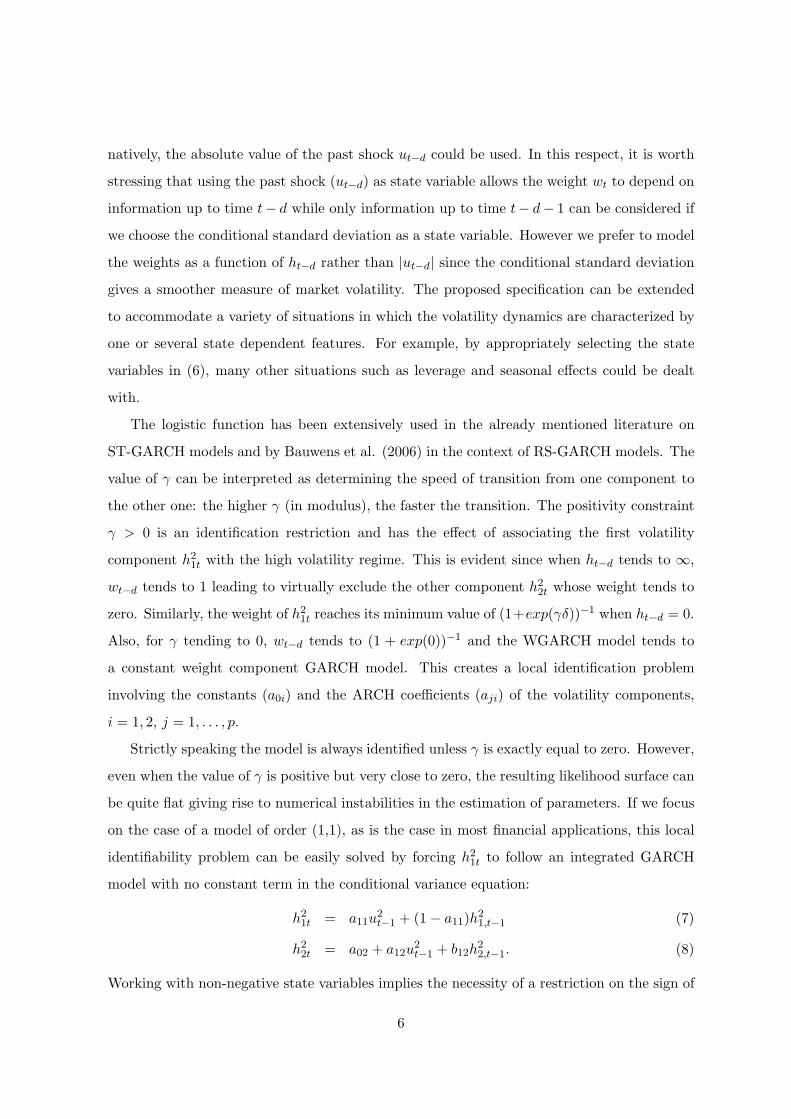
Strictly speaking the model is always identified unless γ is exactly equal to zero. However,
even when the value of γ is positive but very close to zero, the resulting likelihood surface can
be quite flat giving rise to numerical instabilities in the estimation of parameters. If we focus
on the case of a model of order (1,1), as is the case in most financial applications, this local
identifiability problem can be easily solved by forcing h21t to follow an integrated GARCH
model with no constant term in the conditional variance equation:
h21t = a11u
2t−1 + (1− a11)h2
1,t−1 (7)
h22t = a02 + a12u
2t−1 + b12h
22,t−1. (8)
Working with non-negative state variables implies the necessity of a restriction on the sign of
6
δ. From the above discussion it comes out that the weight wt−d reaches its minimum value
of (1 + exp(γδ))−1 when ht−d = 0. Allowing negative values of δ amounts to constrain the
weight of the first volatility component, which is intended to be associated with turbulent
periods, to be greater than 1/2 even when ht−d = 0. For this reason we impose the further
restriction δ > 0.
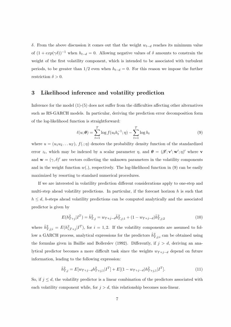
3 Likelihood inference and volatility prediction
Inference for the model (1)-(5) does not suffer from the difficulties affecting other alternatives
such as RS-GARCH models. In particular, deriving the prediction error decomposition form
of the log-likelihood function is straightforward:
`(u; θ) =T∑
t=1
log f(uth−1t ; η)−
T∑
t=1
log ht (9)
where u = (u1u2 . . . uT ), f(.; η) denotes the probability density function of the standardized
error zt, which may be indexed by a scalar parameter η, and θ = (β′;v′;w′; η)′ where v
and w = (γ, δ)′ are vectors collecting the unknown parameters in the volatility components
and in the weight function w(.), respectively. The log-likelihood function in (9) can be easily
maximized by resorting to standard numerical procedures.
If we are interested in volatility prediction different considerations apply to one-step and
multi-step ahead volatility predictions. In particular, if the forecast horizon h is such that
h ≤ d, h-steps ahead volatility predictions can be computed analytically and the associated
predictor is given by
E(h2T+j |IT ) = h2
T,j = wT+j−dh2T,j;1 + (1− wT+j−d)h2
T,j;2 (10)
where h2T,j;i = E(h2
i,T+j |IT ), for i = 1, 2. If the volatility components are assumed to fol-
low a GARCH process, analytical expressions for the predictors h2T,j;i can be obtained using
the formulas given in Baillie and Bollerslev (1992). Differently, if j > d, deriving an ana-
lytical predictor becomes a more difficult task since the weights wT+j−d depend on future
information, leading to the following expression:
h2T,j = E[wT+j−dh
2T+j,1|IT ] + E[(1− wT+j−d)h2
T+j,1|IT ]. (11)
So, if j ≤ d, the volatility predictor is a linear combination of the predictors associated with
each volatility component while, for j > d, this relationship becomes non-linear.
7

The predictor in (11) can be evaluated by Monte Carlo simulation from the estimated
model. However, this approach does not account for parameter uncertainty. Alternatively, it
is possible to resort to the Bayesian approach in order to obtain an estimate of the predictive
density of returns which is integrated over the admissible parameter space. This issue is dealt
with in the next section.
In order to assess the practical relevance of this issue, it is worth discussing the value
typically assumed for the delay d. The value of d is expected to depend on the data collection
frequency. However, if the model is fitted to daily data, it is reasonable to expect relatively
low values of d (d ≤ 5). Hence, the generation of medium (e.g. weekly) and long-term (e.g.
monthly) predictions of volatility will in general require to compute the expectation in (11).
This is a relevant problem for risk managers, since long-term volatility predictions are required
for the computation of some widely used risk measures such as VaR and ES. For example, the
Basle Committee (1996) specifies a multiple of three times the 99% confidence 10-day VaR as
minimum regulatory market risk capital. Also, the Risk Metrics Group (1999) suggests that
the forecast horizon should reflect an institution typical holding period: ”banks, brokers, and
hedge funds tend to look at a 1-day to 1-week worst-case forecast, while longer-term investors,
like mutual and pension funds, may consider a 1-month to 3-month time frame. Corporations
may use up to an annual horizon for strategic scenario analysis”.
4 Bayesian inference for WGARCH models
The complexity of GARCH models renders the derivation of analytical Bayesian inference
results an insurmountable challenge. Hence the application of simulation based techniques is
required. In order to draw a sample from the posterior distribution of the full parameter vector
θ, we implement a Gibbs sampling algorithm with blocks given by θ1 = β and θ2 = (v′;w′; η)′.
For a given prior π(β), the conditional posterior of β is given by
ϕ(β|θ2, IT ) ∝ π(β)
T∏
t=1
f(rt|θ, It−1) (12)
where f(.) indicates the density of rt. Since direct sampling from ϕ(β|θ2, YT ) is not feasible,
we use the Metropolis-Hastings algorithm (Hastings, 1970), choosing a k-dimensional multi-
variate normal distribution as a proposal. The mean and variance of the proposal density
are set equal to the maximum likelihood estimate and the inverse of the associated observed
8

information matrix, respectively. Assuming prior independence, π(β) is factorized as the
product of k uniform marginal densities. At the (j +1)-th iteration, we first generate a (r×1)
pseudo-random vector from the proposal, z(j+1) ∼ ι(z), and compute
p = min
{ϕ(z(j+1))ϕ(β(j))
ι(z(j))ι(β(j+1))
, 1
}. (13)
Then, we accept β(j+1) = z(j+1), with probability p, and take β(j+1) = β(j), with probability
1− p.
Similarly, given a prior density π(θ2), the conditional posterior density of the parameter
vector θ2 is given by:
ϕ(θ2|β, IT ) ∝ π(θ2)T∏
t=1
f(rt|θ, It−1). (14)
To simulate from the density in (14) we use the griddy Gibbs sampler. This algorithm has been
originally proposed by Ritter and Tanner (1992) to solve a bivariate problem while Bauwens
and Lubrano (1998) have successively applied it to the estimation of an asymmetric GARCH
type model including seven parameters. Let us denote by θ(j)2 the value of the parameter
vector sampled at the j-th iteration. At iteration j +1, a draw from the conditional posterior
of θ2 is generated through the following steps:
1. Let v−1 be the vector of volatility parameters excluding its first element a01. Then, use
(14) to evaluate κ(a01|βj ,vj−1,w
j , IT ), which is the kernel of the conditional posterior
density of a01 given β, w and v−1 sampled at iteration j, over a grid (a101, a
201, . . . , a
G01).
The calculated values form the vector Gκ = (κ1, . . . , κG) with κi (i = 1, . . . , G) being
the kernel evaluated at the i-th grid point.
2. By a deterministic integration rule using M points, compute
GΦ = (0, Φ2, . . . , ΦG)
with
Φi =∫ ai
01
a101
κ(a01|βj ,vj−1,w
j , IT )da01 i = 2, . . . , G.
3. Simulate u ∼ U(0, ΦG) and invert Φ(a01|βj ,vj−1,w
j , IT )) by numerical interpolation to
obtain a draw a(j+1)01 ∼ ϕ(a01|β(j)),v(j)−1,w(j), IT ).
9

4. Repeat steps 1-3 for all the other parameters in θ2.
The implementation of the griddy Gibbs sampler requires the definition of suitable integra-
tion intervals for each of the elements in θ2. The definition of the integration intervals plays a
critical role in the procedure and so their determination must be made carefully. The values
of the integration bounds for each parameter are usually tentatively specified and adjusted
in order to cover the region of the parameter space over which the posterior is relevant. The
prior distributions are assumed to be uniform over the chosen intervals for all the parameters
except for γ, the slope coefficient of the weight function.
Following Lubrano (2001), choosing a uniform prior for this parameter leads to a non-
integrable posterior distribution. A similar problem arises for the degrees of freedom param-
eter ν if the errors are assumed to follow a Student’s t distribution, as shown in Bauwens and
Lubrano (1998). In both cases, one possible solution is to assume an uniform prior restricted
over a finite interval where the restriction on the prior domain is automatically implied by the
use of the griddy Gibbs sampler. An alternative choice is to use a truncated Cauchy density
as a prior, which gives:
π(ν) ∝ (1 + ν2)−1 π(γi) ∝ (1 + γ2)−1. (15)
Bauwens and Lubrano (1998) document a very long tail for ν when a flat prior is used while
Lubrano (2001) successfully applies this solution to the estimation of a ST-GARCH model
with a logistic transition function. So, our preference is for a half-Cauchy prior since we expect
this choice to limit the impact on the posterior results of the chosen integration interval.
5 Bayesian prediction of VaR and ES
VaR and ES are two popular measures of market risk commonly used by researchers and risk
managers. If we let RT+h =∑h
i=1 rT+i be the h-period (h > 0) aggregated return, at time T
the h-period VaR at the 100(1 − α)% confidence level, indicated as V aR(α)T,h, can be defined
as the order α quantile of the conditional distribution of RT+h conditional on information at
the time of prediction T :2
P (RT+h < V aR(α)T,h|IT ) = α. (16)
2Our definition of VaR differs from that commonly used in risk management practice since, as an estimate
of VaR, we consider the relevant empirical quantile of the predictive distribution of returns taken with its sign.
10
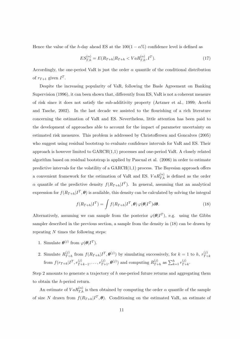
Hence the value of the h-day ahead ES at the 100(1− α%) confidence level is defined as
ES(α)T,h = E(RT+h|RT+h < V aR
(α)T,h, IT ). (17)
Accordingly, the one-period VaR is just the order α quantile of the conditional distribution
of rT+1 given IT .
Despite the increasing popularity of VaR, following the Basle Agreement on Banking
Supervision (1996), it can been shown that, differently from ES, VaR is not a coherent measure
of risk since it does not satisfy the sub-additivity property (Artzner et al., 1999; Acerbi
and Tasche, 2002). In the last decade we assisted to the flourishing of a rich literature
concerning the estimation of VaR and ES. Nevertheless, little attention has been paid to
the development of approaches able to account for the impact of parameter uncertainty on
estimated risk measures. This problem is addressed by Christoffersen and Goncalves (2005)
who suggest using residual bootstrap to evaluate confidence intervals for VaR and ES. Their
approach is however limited to GARCH(1,1) processes and one-period VaR. A closely related
algorithm based on residual bootstrap is applied by Pascual et al. (2006) in order to estimate
predictive intervals for the volatility of a GARCH(1,1) process. The Bayesian approach offers
a convenient framework for the estimation of VaR and ES. V aR(α)T,h is defined as the order
α quantile of the predictive density f(RT+h|IT ). In general, assuming that an analytical
expression for f(RT+h|IT , θ) is available, this density can be calculated by solving the integral
f(RT+h|IT ) =∫
f(RT+h|IT , θ) ϕ(θ|IT )dθ. (18)
Alternatively, assuming we can sample from the posterior ϕ(θ|IT ), e.g. using the Gibbs
sampler described in the previous section, a sample from the density in (18) can be drawn by
repeating N times the following steps:
1. Simulate θ(j) from ϕ(θ|IT ).
2. Simulate R(j)T+h from f(RT+h|IT , θ(j)) by simulating successively, for k = 1 to h, r
(j)T+k
from f(rT+k|IT , r(j)T+k−1, . . . , r
(j)T+1,θ
(j)) and computing R(j)T+h as
∑hk=1 r
(j)T+k.
Step 2 amounts to generate a trajectory of h one-period future returns and aggregating them
to obtain the h-period return.
An estimate of V aR(α)T,h is then obtained by computing the order α quantile of the sample
of size N drawn from f(RT+h|IT , θ). Conditioning on the estimated VaR, an estimate of
11

ES(α)T,h can be computed as
ES(α)
T,h =1
#(RT+h,j < V aR(α)T,h)
∑
j:RT+h,j<V aR(α)T,h
R(j)T+h, (19)
which is the mean of the sampled returns falling below the estimated VaR. So estimates of
VaR and ES for relatively long holding periods are obtained in a straightforward manner
as a by-product of the Gibbs sampling algorithm. This way of computing VaR and ES
has two important advantages. First, it naturally accounts for parameter uncertainty since
the predictive densities of returns are integrated over the parameter space. Second, long
term predictions of volatility and related risk measures can be easily obtained by simulation
independently of the model complexity.
6 An application to daily S&P500 returns
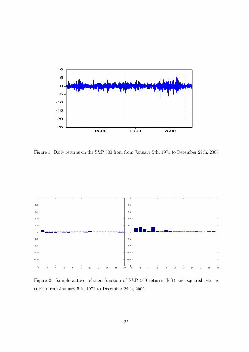
In this section, we present an application to a time series of daily (percentage) log-returns
on the S&P500 stock market index. The observation period goes from January 5, 1971 to
December 29, 2006 for a total of 9086 observations (figure 1). The data are characterized
by a strong kurtosis and a remarkable negative skewness (table 1). The value of the Ljung-
Box Q-statistics provides evidence in favour of the presence of a significant autocorrelation
structure in the returns as well as in the squared returns series. Moreover, visual inspection
of the sample correlogram of the squared returns reveals a highly persistent autocorrelation
pattern (figure 2). In order to account for these features we model the returns rt by a first
order autoregressive model whose residuals follow a WGARCH model of order (1,1):
rt = φ0 + φ1rt−1 + ut (20)
ut = htzt (21)
where ztiid∼ (0, 1) and h2
t is defined as in (4) with p = q = 1. The value of the delay parameter
d has been set equal to 1.
The series has been divided into two subseries including observations from 1 to 8500 and
from 8501 to the end of the observation period, respectively. The first subseries has been
used for model estimation while the second one has been kept for out of sample forecast
12

Table 1: Descriptive statistics and Ljung-Box Q-statistics for the S&P 500 returns (Qr(.))
and squared returns (Qr2(.)). Values in brackets are p-values.
mean s.d. min. max. skew. kur. Qr(10) Qr2(10)
0.0302 0.9906 -22.8997 8.7089 -1.4419 38.6458 51.771(0.0000)
656.55(0.0000)
evaluation. In order to estimate the joint posterior of the AR(1)-WGARCH(1,1) defined in
equations (20)-(21) we have implemented the Gibbs sampler described in section 4 under two
different distributional assumptions for zt, normal and Student’s t.
As a proposal for the Metropolis-Hastings step of the algorithm we have chosen a bivari-
ate normal. The covariance matrix estimated by the observed information matrix has been
multiplied by an inflation factor equal to 1.2 to allow for tails heavier than those implied by
the asymptotic distribution of the maximum likelihood estimator.
In the implementation of the griddy Gibbs sampler for the volatility model parameters,
the integration intervals used for the estimation, as it is usual practice, have been selected by a
trial and error procedure aimed at avoiding sharp truncations in the tails of the marginal pos-
terior distributions while still preserving the positivity of the estimated conditional variance
and its components.
For the normal model, 10000 iterations of the algorithm have been performed. The conver-
gence of the chain has been assessed by using cumsum diagrams. A simple visual inspection of
the plots suggests that, for the normal model (figure 3), convergence is likely to be achieved
after iteration 5000. Hence, only the second half of the chain is used for inference while
the first 5000 draws are discarded. Differently, for the t model (figure 4), since the chain is
converging more slowly than in the normal case, it is necessary to increase the number of
iterations from 10000 to 15000. The first 10000 draws have then been used as burn-in period
for the sampler.
The posterior means and standard deviations based on the adjusted samples are reported
in table 2. In general, the estimated persistence of the first volatility component (figures 5a
and 6a), measured in terms of the sum (a11+b11), is substantially lower than the corresponding
estimate obtained for the second component (figures 5b and 6b). The persistence decrease
is higher for the model with t errors, 0.64 versus 0.98, than for the normal, 0.84 versus 0.99.
13

Other important differences between the two volatility components arise if we consider the
value of the intercept and of the GARCH parameter which turn out to be higher for the first
component, that is the one associated with turbulent periods. Also, in the normal case the
value of the estimated GARCH coefficient is much higher than for the t model reflecting a
higher sensitivity to recent shocks. So it follows that in turbulent periods the volatility tends
to be less persistent and more sensitive to recent shocks. Differently, in tranquil periods
volatility is highly persistent and less sensitive to shocks. In other words, its variation tends
to be mainly driven by long run factors.
Table 2: Posterior means and standard deviations (in brackets) for the normal WGARCH,
t-WGARCH, normal GARCH and t-GARCH models
WGn WGt Gn Gt
φ0 0.0370(0.0087)
0.0390(0.0089)
0.0401(0.0093)
0.0395(0.0089)
φ1 0.0854(0.0110)
0.0833(0.0119)
0.0955(0.0125)
0.0831(0.0121)
a01 0.4433(0.2406)
0.3872(0.2804)
0.0090(0.0019)
0.0049(0.001146)
a11 0.3781(0.1024)
0.1091(0.0615)
0.0685(0.0059)
0.0405(0.0043)
b11 0.4642(0.1030)
0.5332(0.2112)
0.9242(0.0067)
0.9397(0.0062)
a02 0.0050(0.0022)
0.0032(0.0018)
a12 0.0440(0.0104)
0.0398(0.0082)
b12 0.9495(0.0104)
0.9429(0.0082)
γ 6.604(2.9894)
2.737(2.080)
δ 1.449(0.1079)
2.598(1.229)
ν 8.218(0.9338)
8.061(0.6739)
Figures 5c and 6c report the time plots of the weight functions w(.) evaluated at the
estimated posterior means assuming normal and t errors, respectively. In both cases, as
expected, in highly volatile periods the first component virtually excludes the other while
the opposite happens as the market moves back to a tranquil state. High volatility periods,
14

however, are differently identified within the normal and t models. In the t model, the estimate
of the threshold parameter δ turns out to be higher than for the normal model, leading to a
substantial reduction of the average weight of the high volatility component. This implies that
the model completely switches to the high volatility regime only in the period immediately
following the ”black Monday” stock market crash in October 1987.
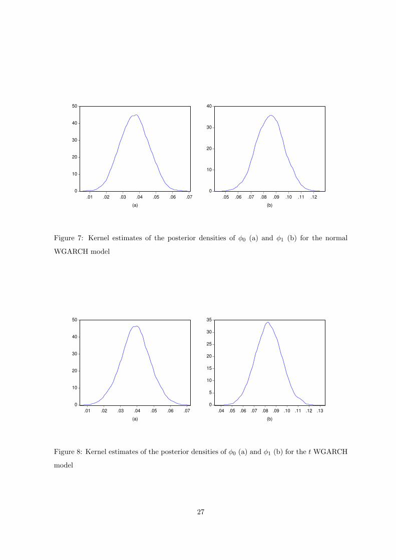
Figures 7 and 8 report the smoothed empirical densities3 of the samples drawn from the
posteriors of the conditional mean parameters φ0 and φ1. The estimated marginal posterior
densities of the volatility model parameters computed by the griddy Gibbs sampler have been
reproduced in figures 9 and 10, respectively. As expected the marginal posterior of the slope
coefficient of the logistic function γ is positively skewed and characterized by a very long tail.
Nevertheless, its mode is far away from zero providing further evidence in favour of the time
varying weights model.
Next, we have applied the estimated WGARCH models for predicting VaR and ES at dif-
ferent horizons (h=1,5,10,15,20) and for different confidence levels (α=0.10,0.05,0.025,0.01).
Also, following Giot and Laurent (2005), long as well as short trading positions have been con-
sidered. VaR and ES predictions have been generated using the simulation based procedure
described in section 5. The performance of the estimated AR-WGARCH models has been
compared to those of two different AR(1) models with GARCH(1,1) errors charaterized by
Student’s t and normal innovations, respectively. Again, inference on the model parameters
has been conducted by the same Bayesian approach described in section 4. The estimated
posterior means and standard deviations are reported in table 2.
In order to assess the quality of VaR predictions we have used the likelihood ratio statistic
proposed by Kupiec (1995) for testing the hypothesis of correct unconditional coverage. By
means of a binomial likelihood, the number of observed VaR exceptions is compared to the
expected number of VaR exceptions under the hypothesis of correct coverage. The empirical
coverages and the associated p-values are reported in table 3. For long trading positions, if
a 1 day holding period is considered, the models with normal errors tend to perform better
but they are outperformed by their counterparts with t errors as the holding period increases.
Overall, the WGARCH model with the t errors appears to offer the best trade-off between
short and medium-long term predictive ability. A different picture arises as we move to con-3The smoothed estimates have been computed by means of an Epanechnikov kernel estimator.
15
sider short positions. All the models perform satisfactorily if we consider a 1 day holding
period but none of them appears to be effective in estimating VaR for longer holding periods.
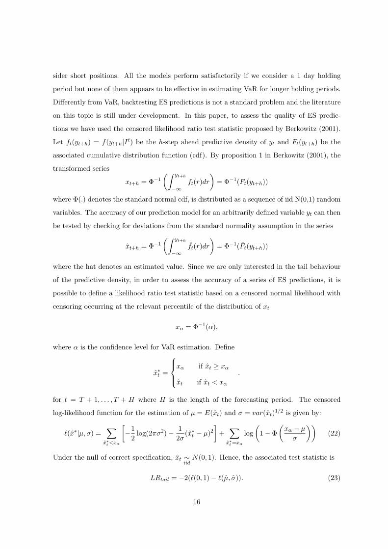
Differently from VaR, backtesting ES predictions is not a standard problem and the literature
on this topic is still under development. In this paper, to assess the quality of ES predic-
tions we have used the censored likelihood ratio test statistic proposed by Berkowitz (2001).
Let ft(yt+h) = f(yt+h|It) be the h-step ahead predictive density of yt and Ft(yt+h) be the
associated cumulative distribution function (cdf). By proposition 1 in Berkowitz (2001), the
transformed series
xt+h = Φ−1
(∫ yt+h
−∞ft(r)dr
)= Φ−1(Ft(yt+h))
where Φ(.) denotes the standard normal cdf, is distributed as a sequence of iid N(0,1) random
variables. The accuracy of our prediction model for an arbitrarily defined variable yt can then
be tested by checking for deviations from the standard normality assumption in the series
xt+h = Φ−1
(∫ yt+h
−∞ft(r)dr
)= Φ−1(Ft(yt+h))
where the hat denotes an estimated value. Since we are only interested in the tail behaviour
of the predictive density, in order to assess the accuracy of a series of ES predictions, it is
possible to define a likelihood ratio test statistic based on a censored normal likelihood with
censoring occurring at the relevant percentile of the distribution of xt
xα = Φ−1(α),
where α is the confidence level for VaR estimation. Define
x∗t =
xα if xt ≥ xα
xt if xt < xα
.
for t = T + 1, . . . , T + H where H is the length of the forecasting period. The censored
log-likelihood function for the estimation of µ = E(xt) and σ = var(xt)1/2 is given by:
`(x∗|µ, σ) =∑
x∗t <xα
[−1
2log(2πσ2)− 1
2σ(x∗t − µ)2
]+
∑
x∗t =xα
log(
1− Φ(
xα − µ
σ
))(22)
Under the null of correct specification, xt ∼iid
N(0, 1). Hence, the associated test statistic is
LRtail = −2(`(0, 1)− `(µ, σ)). (23)
16

The values of µ and σ have been determined by numerical maximization of the log-likelihood
in (22). Under the null, LRtail is asymptotically distributed as a χ22 random variable. A
similar procedure can be defined for the right tail of the distribution (short positions).
Even if a closed form expression for the predictive density is not available, we can simulate
from it using the Gibbs sampler. Namely, let R(j)t+h, j = 1, . . . , N , be a sample from f(Rt+h|It).
We can compute the value of the empirical cdf at any sample point as
F (R(j)t+h|It) =
rank(Rt+h|R(1)t+h, . . . , R
(N)t+h)
N + 1
where Rt+h is the h-period ahead cumulated return at time t and rank(x|y(1), . . . , y(N))
denotes the rank of x in the sample {y(1), . . . , y(N)}. We can then apply the test statistic in
(23) to the normal transformation of the empirical cdf. It must be stressed that the LRtail
statistic does not allow to directly test the accuracy of the ES prediction but provides an
assessment of the accuracy globally achieved in fitting the tails of the predictive density.
The results of the censored likelihood ratio test (table 4) are in line with what observed for
VaR prediction. For a holding period of 1 day and for long positions, the t GARCH model is
outperformed by the normal WGARCH and GARCH models. Normal models, however, are
not accurate at predicting ES for longer holding periods. Again, the WGARCH model with t
errors appears to offer a reasonable trade-off. It performs satisfactorily in predicting the ES
for a 1 day holding period while still providing accurate longer term prediction of the ES. For
what concerns short trading positions, all the models are sufficiently accurate in predicting ES
1 day ahead while, again, for longer holding periods none of the models considered performs
satisfactorily. For holding periods ≥ 5, we have not reported the value of the LRtail test
for α = 0.01. In these cases, due to the highly conservative nature of the associated VaR
estimates, only a reduced number of points was found to fall below the threshold x0.01 in (22).
Hence the test is likely to be not accurate since the available sample from xt does not provide
sufficient information for reconstructing its extreme tail behaviour.
7 Concluding remarks
The WGARCH model discussed in this paper allows to reproduce state dependent volatility
dynamics without suffering from the limitations which typically complicate inference from
other alternatives such as RS-GARCH models.
17

To investigate the effectiveness of WGARCH models in standard risk management appli-
cations, we have presented an application of the proposed modelling strategy to the prediction
of VaR and ES for a time series of daily returns on the S&P 500. The empirical results show
that the predictive performance of a WGARCH model with t errors favourably compares with
that of standard GARCH models. In order to further improve the ability of WGARCH models
to reproduce the tail behaviour of asset returns, it could be of interest considering skewed er-
ror distributions such as the Skew t distribution investigated by Bauwens and Laurent (2005).
Finally, another important topic for future research is related to the investigation of the statis-
tical properties of WGARCH models such as implied moments and volatility autocorrelation
structure.
18

References
Acerbi, C., Tasche, D. (2002) On the coherence of Expected Shortfall, Journal of Banking
and Finance, 26(7), 1487-1503.
Artzner, P., Delbaen, F., Eber, J.-M., Heath, D. (1999) Coherent measures of risk, Math-
ematical Finance, 9(3), 203228.
Baillie, R.T., Bollerslev, T. (1992) Prediction in Dynamic Models with Time Dependent
Conditional Variances, Journal of Econometrics, 52, 91–113.
Bank for International Settlements (1996) Basle Committee on Banking Supervision.
Amendment to the Capital Accord to incorporate market risks.
Bauwens, L., Laurent, S. (2005) A new class of multivariate skew densities, with applica-
tion to GARCH models, Journal of Business and Economic Statistics, 23(3), 346-354.
Bauwens, L., Lubrano, M. (1998) Bayesian inference on GARCH models using the Gibbs
sampler,Econometrics Journal, 1, pages C23-C46.
Bauwens, L., Preminger, A., Rombouts, J. V. K. (2006) Regime switching GARCH mod-
els, CORE Discusion Paper, 2006/11.
Berkowitz, J. (2001) Testing density forecasts with applications to risk management, Jour-
nal of Business & Economic Statistics, 19, 4, 465–474.
Christoffersen, P., Goncalves, S. (2005) Estimation Risk in Financial Risk Management,
Journal of Risk, 7, 1–28.
Ding, Z., Granger, C. W. J. (1996) Modeling volatility persistence of speculative returns:
a new approach, Journal of Econometrics, 73, 185–215.
Engle, R. F., Lee, G. G. J. (1999) A Long-Run and Short-Run Component Model of Stock
Return Volatility, in Cointegration, Causality, and Forecasting (Engle R. F. and White
H., eds.), Oxford University Press.
Giot, P., Laurent, S. (2003) Value-at-Risk for long and short trading positions, Journal
of Applied Econometrics,18, 641-664.
19
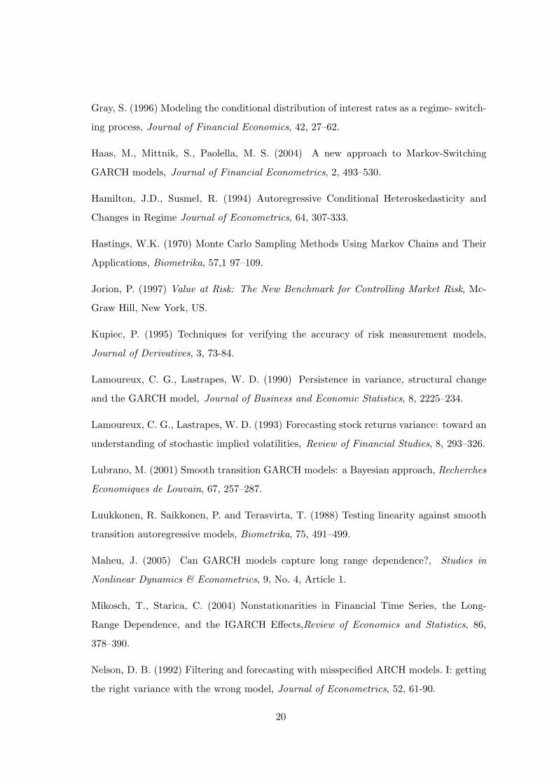
Gray, S. (1996) Modeling the conditional distribution of interest rates as a regime- switch-
ing process, Journal of Financial Economics, 42, 27–62.
Haas, M., Mittnik, S., Paolella, M. S. (2004) A new approach to Markov-Switching
GARCH models, Journal of Financial Econometrics, 2, 493–530.
Hamilton, J.D., Susmel, R. (1994) Autoregressive Conditional Heteroskedasticity and
Changes in Regime Journal of Econometrics, 64, 307-333.
Hastings, W.K. (1970) Monte Carlo Sampling Methods Using Markov Chains and Their
Applications, Biometrika, 57,1 97–109.
Jorion, P. (1997) Value at Risk: The New Benchmark for Controlling Market Risk, Mc-
Graw Hill, New York, US.
Kupiec, P. (1995) Techniques for verifying the accuracy of risk measurement models,
Journal of Derivatives, 3, 73-84.
Lamoureux, C. G., Lastrapes, W. D. (1990) Persistence in variance, structural change
and the GARCH model, Journal of Business and Economic Statistics, 8, 2225–234.
Lamoureux, C. G., Lastrapes, W. D. (1993) Forecasting stock returns variance: toward an
understanding of stochastic implied volatilities, Review of Financial Studies, 8, 293–326.
Lubrano, M. (2001) Smooth transition GARCH models: a Bayesian approach, Recherches
Economiques de Louvain, 67, 257–287.
Luukkonen, R. Saikkonen, P. and Terasvirta, T. (1988) Testing linearity against smooth
transition autoregressive models, Biometrika, 75, 491–499.
Maheu, J. (2005) Can GARCH models capture long range dependence?, Studies in
Nonlinear Dynamics & Econometrics, 9, No. 4, Article 1.
Mikosch, T., Starica, C. (2004) Nonstationarities in Financial Time Series, the Long-
Range Dependence, and the IGARCH Effects,Review of Economics and Statistics, 86,
378–390.
Nelson, D. B. (1992) Filtering and forecasting with misspecified ARCH models. I: getting
the right variance with the wrong model, Journal of Econometrics, 52, 61-90.
20

Pascual, L., Romo, J., Ruiz, E. (2006) Bootstrap Prediction for Returns and Volatilities
in GARCH Models, Computational Statistics & Data Analysis, 50, 2293-2312.
Risk Metrics Group (1999) Risk Management: A Practical Guide, www.riskmetrics.com.
Ritter, C., Tanner, M. A. (1992) Facilitating the Gibbs Sampler: The Gibbs Stopper and
the Griddy-Gibbs Sampler, Journal of the American Statistical Association, 87, 861–868.
21
-25
-20
-15
-10
-5
0
5
10
2500 5000 7500
Figure 1: Daily returns on the S&P 500 from from January 5th, 1971 to December 29th, 2006
0 2 4 6 8 10 12 14 16 18 20−1
−0.8
−0.6
−0.4
−0.2
0
0.2
0.4
0.6
0.8
1
0 2 4 6 8 10 12 14 16 18 20−1
−0.8
−0.6
−0.4
−0.2
0
0.2
0.4
0.6
0.8
1
Figure 2: Sample autocorrelation function of S&P 500 returns (left) and squared returns
(right) from January 5th, 1971 to December 29th, 2006
22

Figure 3: Cumsum diagrams with ±5% bands for the normal WGARCH model. From left to
right and from top to bottom: φ0,φ1,a01,a11,b11,a02,a12,b12,δ, γ.
23

Figure 4: Cumsum diagrams with ±5% bands for the t WGARCH model. From left to right
and from top to bottom: φ0,φ1,a01,a11,b11,a02,a12,b12,δ, γ, ν.
24

Figure 5: First volatility component (h21t, a), second volatility component (h2
2t, b), weights
series (wt, c) from the normal WGARCH model
25

Figure 6: First volatility component (h21t, a), second volatility component (h2
2t, b), weights
series (wt, c) from the t-WGARCH model
26
0
10
20
30
40
50
.01 .02 .03 .04 .05 .06 .07
(a)
0
10
20
30
40
.05 .06 .07 .08 .09 .10 .11 .12
(b)
Figure 7: Kernel estimates of the posterior densities of φ0 (a) and φ1 (b) for the normal
WGARCH model
0
10
20
30
40
50
.01 .02 .03 .04 .05 .06 .07
(a)
0
5
10
15
20
25
30
35
.04 .05 .06 .07 .08 .09 .10 .11 .12 .13
(b)
Figure 8: Kernel estimates of the posterior densities of φ0 (a) and φ1 (b) for the t WGARCH
model
27

Figure 9: Estimated marginal posteriors of the parameters of the volatility model for the
normal WGARCH model. From left to right and from top to bottom: a01,a11,b11,a02,a12,b12,δ,
γ.
28

Figure 10: Estimated marginal posteriors of the parameters of the volatility model for the t
WGARCH model. From left to right and from top to bottom: a01,a11,b11,a02,a12,b12,δ, γ, nu.
29

Table 3: Out-of-sample empirical coverages of the normal WGARCH (WGn), t-WGARCH
(WGt), normal GARCH (Gn) and t-GARCH (Gt) models for different confidence levels (α),
horizons, long (L) and short (S) positions. Values in brackets are p-values of Kupiec’s likeli-
hood ratio test statistic for correct unconditional coverage
Long positions Short positions
α WGn WGt Gn Gt WGn WGt Gn Gt hor.
0.10 0.0921(0.5215)
0.1399(0.0022)
0.0921(0.5215)
0.1502(0.0001)
0.0819(0.1331)
0.1212(0.0972)
0.0836(0.1749)
0.1263(0.0407)
1d
0.05 0.0392(0.2154)
0.0648(0.1141)
0.0444(0.5240)
0.0751(0.0093)
0.0430(0.4036)
0.0631(0.1601)
0.0392(0.2154)
0.0631(0.1601)
0.025 0.0205(0.4694)
0.0307(0.3918)
0.0205(0.4694)
0.0410(0.0233)
0.0256(0.9265)
0.0358(0.1143)
0.0256(0.9265)
0.0375(0.0699)
0.01 0.0085(0.7142)
0.0153(0.2269)
0.0085(0.7142)
0.0190(0.0571)
0.0085(0.7142)
0.0119(0.6461)
0.0068(0.4127)
0.0154(0.2269)
0.10 0.0722(0.0191)
0.1065(0.6030)
0.0773(0.0585)
0.1092(0.5122)
0.0412(0.0000)
0.0687(0.0080)
0.0378(0.0000)
0.0722(0.0191)
5d
0.05 0.0292(0.0129)
0.0515(0.8647)
0.0309(0.0235)
0.0584(0.3635)
0.0086(0.0000)
0.0240(0.0015)
0.0069(0.0000)
0.0275(0.0066)
0.025 0.0120(0.0260)
0.0240(0.8832)
0.0069(0.0009)
0.0292(0.5262)
0.0017(0.0000)
0.0034(0.0000)
0.0017(0.0000)
0.0069(0.0009)
0.01 0.0016(0.0131)
0.0069(0.4217)
0.0017(0.0131)
0.0069(0.4217)
0.0000(.)
0.017(0.0131)
0.0000(.)
0.0017(0.0131)
0.10 0.0503(0.0000)
0.0901(0.4219)
0.0573(0.0000)
0.1023(0.8573)
0.0156(0.0000)
0.0485(0.0000)
0.0156(0.0000)
0.0537(0.0001)
10d
0.05 0.0191(0.0001)
0.0364(0.1158)
0.0191(0.0001)
0.0433(0.4521)
0.0069(0.0000)
0.0121(0.0000)
0.0156(0.0000)
0.0121(0.0000)
0.025 0.0104(0.0111)
0.0173(0.2121)
0.0104(0.0111)
0.0208(0.5056)
0.0035(0.0000)
0.0052(0.0002)
0.0156(0.0000)
0.0069(0.0010)
0.01 0.0052(0.2018)
0.0087(0.7416)
0.0052(0.2018)
0.0104(0.9238)
0.0017(0.0137)
0.0035(0.0682)
0.0000(.)
0.0035(0.0682)
0.10 0.0524(0.0000)
0.0891(0.3796)
0.0507(0.0000)
0.0909(0.4624)
0.0210(0.0000)
0.0402(0.0000)
0.0140(0.0000)
0.0332(0.0000)
15d
0.05 0.01075(0.0000)
0.0402(0.2667
0.0122(0.0000)
0.0437(0.4807)
0.0052(0.0000)
0.0140(0.0000)
0.0052(0.0000)
0.0140(0.0000)
0.025 0.0035(0.0000)
0.0140(0.0661)
0.0017(0.0000)
0.0157(0.1281)
0.0035(0.0000)
0.0052(0.0002)
0.0035(0.0000)
0.0052(0.0002)
0.01 0.0000(.)
0.0000(.)
0.0000(.)
0.0017(0.0144)
0.0000(.)
0.0035(0.0709)
0.0000(.)
0.0035(0.0709)
0.10 0.0564(0.0002)
0.0917(0.5052)
0.0529(0.0002)
0.0970(0.8111)
0.0176(0.0000)
0.0353(0.0000)
0.0176(0.0000)
0.0335(0.0000)
20d
0.05 0.0106(0.0000)
0.0423(0.3898)
0.0106(0.0000)
0.0441(0.5104)
0.0053(0.0000)
0.0159(0.0000)
0.0035(0.0000)
0.0159(0.0000)
0.025 0.0035(0.0000)
0.0106(0.0131)
0.0000(.)
0.0106(0.0131)
0.0000(.)
0.0053(0.0003)
0.0000(.)
0.0088(0.0044)
0.01 0.0000(.)
0.0018(0.0151)
0.0000(.)
0.0035(0.0738)
0.0000(.)
0.0000(.)
0.0000(.)
0.0000(.)
30

Table 4: Out-of-sample predictive densities estimated by WGARCH (WGn), t WGARCH
(WGt), normal GARCH (Gn) and t-GARCH (Gt) models. Values in brackets are p-values
associated with the censored likelihood ratio test statistic proposed by Berkowitz (2001).
Long positions Short positions
α WGn WGt Gn Gt WGn WGt Gn Gt hor.
0.10 0.3646(0.8333)
4.343(0.1140)
0.1882(0.9102)
6.315(0.0425)
0.9727(0.6149)
1.274(0.5288)
0.8417(0.6565)
1.947(0.3778)
1d
0.05 0.6722(0.7145)
1.218(0.5439)
0.2097(0.9004)
3.006(0.2224)
0.3235(0.8506)
1.004(0.6053)
0.8974(0.6384)
0.9356(0.6264)
0.025 0.2217(0.8951)
0.4455(0.8003)
0.3813(0.8264)
2.451(0.2937)
0.5845(0.7466)
1.708(0.4257)
0.3193(0.8524)
1.679(0.4319)
0.01 0.1323(0.9360)
2.094(0.3511)
0.1286(0.9377)
2.278(0.3201)
0.3611(0.8348)
0.8112(0.6666)
0.3204(0.8520)
1.572(0.4557)
0.10 3.496(0.1741)
0.3044(0.8588)
4.064(0.1311)
0.2523(0.8815)
17.790(0.0001)
7.383(0.0249)
18.900(0.0001)
5.932(0.0675)
5d
0.05 3.198(0.2021)
0.2321(0.8904)
4.454(0.1079)
0.7378(0.6915)
16.140(0.0003)
7.289(0.0261)
16.450(0.0003)
5.150(0.0761)
0.025 2.761(0.2515)
0.3225(0.8511)
4.971(0.0833)
1.339(0.5121)
9.923(0.0070)
7.716(0.0211)
9.941(0.0070)
5.286(0.0714)
0.10 8.483(0.0144)
0.5457(0.7612)
7.993(0.0184)
0.3576(0.8363)
29.690(0.0000)
11.490(0.0032)
29.880(0.0000)
9.291(0.0096)
10d
0.05 6.484(0.0391)
1.079(0.5830)
6.557(0.0377)
0.2357(0.8888)
15.190(0.0005)
10.730(0.0047)
15.320(0.0005)
10.890(0.0043)
0.025 2.758(0.2518)
0.7127(0.7002)
2.869(0.2383)
0.0185(0.9115)
7.455(0.0240)
5.959(0.0508)
7.642(0.0022)
4.739(0.0935)
0.10 11.530(0.0031)
2.199(0.3330)
13.700(0.0011)
1.835(0.3996)
26.720(0.0000)
14.530(0.0007)
31.060(0.0000)
16.240(0.0003)
15d
0.05 10.070(0.0065)
2.994(0.2238)
13.140(0.0014)
2.865(0.2387)
16.820(0.0002)
9.488(0.0087)
16.830(0.0002)
9.388(0.0091)
0.025 8.645(0.0133)
3.279(0.1941)
10.330(0.0057)
3.207(0.2012)
7.453(0.0241)
5.833(0.0541)
7.467(0.0239)
6.024(0.0492)
0.10 12.830(0.0016)
2.373(0.3052)
16.450(0.0003)
2.232(0.3276)
28.170(0.0000)
16.630(0.0003)
30.220(0.0000)
16.010(0.0003)
20d
0.05 12.690(0.0018)
4.344(0.1140)
14.050(0.0009)
4.166(0.1245)
18.630(0.0001)
9.185(0.0103)
22.210(0.0000)
8.376(0.0152)
0.025 9.234(0.0099)
3.683(0.1586)
12.470(0.0020)
3.395(0.1831)
12.470(0.0020)
7.408(0.0246)
12.470(0.0002)
6.409(0.0406)
31