l adaptive control of hysteresis in smart materials · l1 adaptive control of hysteresis in smart...

L1 Adaptive Control of Hysteresis in Smart Materials

Xiang Fan∗ and Ralph C. Smith†

Center for Research in Scientific ComputationDepartment of Mathematics

North Carolina State UniversityRaleigh, NC 27695

ABSTRACT

Smart materials display coupling between electrical, magnetic, thermal and elastic behavior. Hence these mate-rials have inherent sensing and actuation capacities. However, the hysteresis inherent to smart materials presentsa challenge in control of these actuators/sensors. Inverse compensation is a fundamental approach to cope withhysteresis, where one aims to cancel out the hysteresis effect by constructing a right inverse of the hysteresis. Theperformance of the inverse compensation is susceptible to model uncertainties and to error introduced by inexactinverse algorithms. We employ a mathematical model for describing hysteresis. On the basis of the hysteresismodel, a robust adaptive inverse control approach is presented, for reducing hysteresis. The asymptotic trackingproperty of the adaptive inverse control algorithm is proved and the issue of parameters convergence is discussedin terms of the reference trajectory. Moreover, sufficient conditions under which parameter estimates convergeto their true values are derived. Simulations are used to examine the effectiveness of the proposed approach.

Keywords: smart materials, hysteresis, inverse compensation, L1 adaptive control

1. INTRODUCTION

The role of smart materials continues to be critical to technology development in many biomedical, aerospace,and industrial applications. These materials provide advantages in applications where large forces and small dis-placements are desired over a broad frequency range with high precision. A large number of these applicationsemploy piezoelectric or magnetostrictive materials which respectively possess electric or magnetic field induceddisplacement and force. Although smart materials have been successfully implemented in a number of applica-tions, limitations associated with nonlinear and hysteretic behavior have presented challenges in developing highperformance actuation responses over a broad frequency range. The nonlinear and hysteretic behavior is primar-ily due to the reorientation of local electric or magnetic variants that align with the applied electric or magneticfields. Moderate to large field levels can induce 0.1% strain in PZT and up to 6% strain in shape memory alloys.At these fields levels, however, obtaining accurate and precise control is greatly complicated by nonlinearitiesand hysteresis. This has motivated research in developing new control designs that can effectively compensatefor nonlinearities and hysteresis induced by ferroelectric or ferromagnetic switching while still providing accurateforces or displacement over a broad frequency range.

Two general strategies are typically considered when developing a control design to compensate for hysteresis.One approach is to implement a nonlinear inverse compensator which approximately linearizes the constitutivebehavior so that linear control methods can be employed. This approach provides the ability to implement linearcontrol laws; however, this advantage is only realized if the constitutive model is efficient enough to be invertedin real time. The second strategy entails direct incorporation of the material model into the control design sothat the nonlinear control input is directly determined. This circumvents issues associated with computing theconstitutive inverse law, but introduces challenges in identifying robust numerical algorithms that can achieveconvergence efficiently.

∗E-mail: [email protected];†E-mail: [email protected], Telephone: 919-515-7552

1

Both of these approaches require an efficient and accurate constitutive model that can predict the hysteresisbehavior. In the analysis presented here, a homogenized model is implemented which utilizes fundamentalenergy relations at the mesoscopic scale to quantify macroscopic behavior in materials. This modeling frameworkhas been successful in accurately quantifying rate-dependent major an minor hysteresis loops in ferroelectric,magnetostrictive and shape memory alloy; see [4] for details. The first strategy is presented here where theinverse compensator is directly incorporated into the control design.

2. MODEL DEVELOPMENT

The model employed in the present analysis incorporates mesoscopic material behavior at the domain in astochastic homogenization framework to predict macroscopic material behavior. A distribution of interactionfields and coercive fields is implemented to model polarization switching processes that typically occur in thepresence of material in homogeneities and residual fields. Boltzmann relations are included to model thermalrelaxation behavior when thermal energy affects polarization switching. Macroscopic material behavior is deter-mined by homogenizing the local polarization variants according to the distribution of interaction and coercivefields.

2.1. Homogenized Energy Model

The equations governing the homogenized energy model are summarized here. A detailed review of themodeling framework is given in [4]. The homogenized energy model is based on an energy description at themesoscopic length scale. This local energy formulation is used to predict macroscopic behavior using a stochasticrepresentation of material inhomogeneities.

For ferroelectric materials, the Gibbs free energy at the mesoscopic length scale is

G = ψ − EP (2.1)

where ψ is the Helmholtz energy approximated by the piecewise quadratic function

ψ(P ) =

η(P + PR)2/2, P ≤ −PI

η

2(PI − PR)

(P 2

PI− PR

), |P | < PI

η(P − PR)2/2, P ≥ PI

(2.2)

Here E is the electric field, P is the polarization, PI denotes the positive inflection point at which the switchoccurs, PR is the local remanence polarization and η is the reciprocal slope ∂E

∂P . The one-dimensional Helmholtzenergy function is double-well potential below the Curie point Tc which gives rise to a stable spontaneouspolarization with equal magnitude in the positive and negative directions. More details can be found in [4].

The Boltzmann relation gives rise to the local expected values

〈P+〉 =

∫∞PI

exp(−G(E + EI , P )V/kT )dP∫∞PI

P exp(−G(E + EI , P )V/kT )dP(2.3)

〈P−〉 =

∫ −PI

−∞ exp(−G(E + EI , P )V/kT )dP∫ −PI

∞ P exp(−G(E + EI , P )V/kT )dP(2.4)

of the polarization associated with positive and negatively oriented dipoles, respectively. Here V is the volumeof the mesoscopic layer, k is Boltzmann’s constant, and T is the temperature.

The local polarization variants are defined by a volume fraction of variants x+ and x− having positive andnegative orientations, respectively. The relation x− + x+ = 1 must hold for the volums fraction of polarizationvariants.

2

The resulting local average polarization is qualified by the relation

P = x+〈P+〉+ x−〈P−〉. (2.5)

The macroscopic polarization is computed from the distribution of local variants from the relation

[P (E)](t) =∫ ∞

−∞

∫ ∞

0

νc(Ec)νI(EI)P (E + EI ;Ec;x+)dEIdEc (2.6)

where ν(Ec), ν(EI) respectively denote the distributions of coercive field value Ec (at which a dipole changes itsorientations) and interaction field value EI , x+ represents the distribution of the local variants. The densitiescan often be modeled as lognormal or normal distributions. However, when more accurate model predictions arecritical, a general density can be fit to data. As detailed in [4], the model for magnetic material is equivalent.

2.2. Inverse CompensatorAs discussed in Section 1, one method to accurately control a smart material actuator involves the use of aninverse compensator. A prototypical setup for this type for control is depicted in Figure 1. The material isnonlinear, hysteretic, and time-varying, but these attributes are approximately linearized by the inverse filterH−1. The composite system to be controlled is then approximately linear and time-invariant. This allows simplecontrol designs to be utilized, including the L1 control method employed later.

-desired ud

H−1(ud) -field orVoltage

InverseCompensator

Device

H(v) - G(s)u

-Magnetizationor Displacement

Figure 1. Plant with an input nonlinearity.

The inverse compensator is the inverse of the homogenized energy model. Given a value for the polarization(or magnetization), we want to determine the field level necessary to bring the actuator to that value. Moreprecisely, given any valid state x+ and any P within the operating range of the material, determine E such thatP = P , where P is the solution of (2.6). Due to the nonlinearity and dependence on x+, it is not feasible to invert(2.6) analytically. Thus, the problem is reformulated as a numerical root finding problem, namely determiningthe value E such that for a given x+ and P ,

P (E; x+)− P = 0, (2.7)

more details can be found in [1].

3. L1 CONTROL ARCHITECTURE

Consider the system dynamic:

x(t) = Ax(t) + bu(t), x(t0) = x0

y(t) = cT x(t)(3.1)

where x = [x, x]T is the system state vector.

Note thatA may be unknown and we assume that there exists a Hurwitz Am ∈ Rn×n and a vector of idealparameter θ ∈ Rn such that (Am, b) is controllable and A − Am = b θT . We further assume the unknown

3

parameter θ belongs to a given compact convex set Θ. The signal u(t) = [H(v)](t) includes the output of theinverse compensator where v(t) is defined as the electric field; i.e.,

u = [H(v)](t) = [HH−1(ud)](t) (3.2)

where signal ud(t) is used as the input of the inverse compensator H−1(·) to generate the control v(t) which isthen applied to the device, as shown in Fig. 1.

Since the hysteresis inverse [H−1(ud)](t) can not exactly approximate the real inverse of [H(v)](t), we canwrite

u(t) = ud(t) + σ(t) (3.3)

where σ(t) is the inversion error introduced by the inverse compensator. Note that the inversion error can bebounded in magnitude; i.e., |σ(t)| ≤ ∆0 ∈ R. Hence we can model the inversion error as an external disturbanceand attenuate its impact by robust control techniques.

Substituting (3.3) into (3.1) yields

x(t) = Amx(t) + b(ud(t) + θT x(t) + σ(t)),

y(t) = cT x(t).(3.4)

The objective is to design a low-frequency adaptive controller ud(t) such that y(t) tracks a given boundedreference signal r(t) while all other error signals remain bounded.

The elements of the L1 adaptive controller are introduced next.

State Predictor: Consider the state predictor

˙x(t) = Amx(t) + b(ud(t) + θT x(t) + σ(t)),

y(t) = cT x(t).(3.5)

which has the same structure as the system in (3.4). The only difference is that the unknown parametersθ(t), σ(t) are replaced by their adaptive estimated θ(t), σ(t) that are governed the following adaptation laws.

Adaptive Laws: Adaptive estimates are defined via the projection operator:

˙θ(t) = ΓcProj (θ(t), −x(t)xT (t)Pb), θ(0) = 0

˙σ(t) = ΓcProj (σ(t), −xT (t)Pb), σ(0) = 0(3.6)

where x(t) = x(t)− x(t) is the error between the states of the system and the predictor, P is the solution of thealgebraic Lyapunov equation AT

mP + PAm = −Q, Q > 0.

Control Law: The control signal ud(t) is generated through gain feedback of the system

X (s) = D(s)r(s), ud(s) = −kX (s), (3.7)

where k ∈ R+ is a feedback gain, r(s) is the Laplace transformation of

r(t) = ud(t) + θT x(t) + σ(t)− kgr(t), kg = − 1cT A−1

m b(3.8)

and D(s) is a transfer function that leads to strictly proper stable

C(s) =kD(s)

1 + kD(s)(3.9)

with low-pass gain C(0) = 1.

4

L1-gain stability requirement: Design D(s) and k to satisfy

‖G(s)‖L1L < 1, L = maxθ∈Θ

n∑

i=1

|θi(t)| (3.10)

where G(s) = (sI−Am)−1b(1− C(s)), and L1 gain for a stable proper m input n output transfer function, sayG(s), is defined as

‖G(s)‖L1 = maxi=1,··· ,n

m∑

j=1

∫ ∞

0

|gij(t)|dt

where gij(t) is the impulse response of Gij(s), the ith row jth column element of G(s).

In case of of constant θ(t), the stability requirement can be simplified. For the specific choice of D(s) = 1/s,

which yields C(s) =k

s + k, the stability requirement is reduced to

Ag =

[Am + b θT b

−kθT −k

]

being Hurwitz for all θ ∈ Θ.

The close-loop system with it is illustrated in Figure 2.

- H−1 H G(s)

?

Plant

v u xud

ª- State Predictor -x -x

¾Adaptive Law

?

ud + θt x + σ

θT , σ

- D(s) -

¾ud = −kX (s)

6ud

X

Control Law with Low-pass filter

Figure 2. Closed-loop system with the L1 adaptive controller.

5

Note that when C(s) = 1, ud reduces to the ideal control signal

uid(t) = kgr(t)− θT xid − σ(t) (3.11)

and (3.11) is the one that leads to desired system response

xid(t) = Amxid(t) + bkgr(t) (3.12)

by canceling the uncertainties exactly. In the closed-loop predictor system (3.5)− (3.7), uid(t) is further low-passfiltered by C(s) in (3.9) to have guaranteed low-frequency range. Thus, the system in (3.5)− (3.7) has a differentresponse as compared to (3.12) achieved with (3.11). It has been proved in [2] that the response of the statepredictor (3.6) can be made as close as possible to the response of the ideal system (3.12) by reducing ‖G(s)‖L1

arbitrarily small, and ‖G(s)‖L1 can be made arbitrarily small by appropriately choosing the design constants,further details may be found in [2] and [3].

4. SIMULATION

Consider the dynamic system in (3.1) with A =[0 15 7

], b =

[01

], c =

[10

]and the state predictor in (3.5)

with Am =[

0 1−5 −3

]and θ =

[1010

].

We note that A has poles in the right half plane and hence it is an unstable non-minimum phase system.The constant θ is assumed to be unknown and the compact set can be conservatively chosen as Ω = θ1 ∈[0, 20], θ2 ∈ [0, 20]. The control objective is to design an adaptive controller ud(t) to ensure that x1(t) tracksany reference signal r(t) both in transient and steady state.

For implementation of the L1 adaptive controller (3.5), (3.6), (3.7), we need to verify the L1 stability require-ment in (3.10). For constant θ =

[10 10

]T , we have

Ag =

[Am + bθT b

−kθT −k

]=

0 1 05 7 1

−10k −10k −k

. (4.1)

Note that for k > 50, the matrix Ag is Hurwitz. We set k = 100, which means that the transfer function for thelow-pass filter takes the form

Gfil(s) =100

s + 100=

1s

ω0+ 1

, ω0 = 100. (4.2)

Figure 3(a) illustrates the bode plot for the transfer function (4.2).

The bode magnitude plot tells us that at the break frequency, ω = ω0 = 102 rad/sec, the gain is about 3.01dB and the phase is −π

4 degree. At lower frequencies, ω ¿ ω0, the gain is approximatly zero, and at higherfrequencies, ω À ω0, the gain increases at 20 dB/decades and goes through the break frequency at 0 dB; that is,for every factor of 10 increase in frequency, the magnitude drops by 20 dB. We can thus say that the low-passfilter (4.2) we use can pass all signals with frequencies lower than the break frequency 102 rad/sec, and attenuates(reduces the amplitude of) signals with frequencies higher than 102 rad/sec (Note that 1 Hz=2π rad/sec).

Similarly, we can write the transfer function of the reference model (3.13) as:

Gref (s) =5

s2 + 3s + 5=

1(s

ω0

)2

+ 2ζ

(s

ω0

)+ 1

, ω0 =√

5, ζ = h3

2√

5(4.3)

Figure 3(b) illustrates the bode plot for the transfer function (4.3).

6

−40

−35

−30

−25

−20

−15

−10

−5

0

Mag

nitu

de (

dB)

100

101

102

103

104

−90

−45

0

Pha

se (

deg)

Bode DiagramGm = Inf , Pm = −180 deg (at 0 rad/sec)

Frequency (rad/sec)

−80

−60

−40

−20

0

20

Mag

nitu

de (

dB)

10−1

100

101

102

−180

−135

−90

−45

0

Pha

se (

deg)

Bode DiagramGm = Inf dB (at Inf rad/sec) , Pm = 143 deg (at 1 rad/sec)

Frequency (rad/sec)

(a) (b)

Figure 3. Bode diagram; (a) Low-pass filter, (b) the reference model.

We can read from the bode magnitude plot that at the frequencies higher than the break frequency, ω0 =√

5rad/sec, the gain increases at 40 dB/decades and goes through the break frequency at 0 dB; that is, for everyfactor of 10 increase in frequency, the magnitude drops by 40 dB. At lower frequencies, ω ¿ ω0, the gain isapproximately zero and a peak occurs in the magnitude plot near the break frequency ω0. The peak has amagnitude of

|Gref (jωr)| = −20 lg(2ζ√

1− ζ2) = 0.004 dB ∼ 0

where ωr = ω0

√1− 2ζ2 = 0.7.

To solve the ODE system (3.5)− (3.7), we consider two techniques: use of the MATLAB routine ode15s andan implicit Euler technique.

4.1. ODE15s

We first consider a single-frequency sinusoidal function r(t) = cos(t). The frequency of r(t) is 1/2π Hz (= 1rad/sec), based on the above analysis, this r(t) could pass the filter and reference model unchanged. Theoretically,the tracking output x1(t) should exactly match the shape of r(t) = cos(t) after x1(t) converges. Simulation resultsare shown in Figure 4(a). We note that the system output x1(t) converges to r(t) asymptotically whereas x1(t)lags behind the reference signal r(t) with delay time of about t0 = 0.62 sec. The system output x1(t) and predictoroutput x1(t) are almost the same. To cancel out the delay, we could redefine r(t) by r(t+ t0) , so it requires thatwe should have an exact prediction of the time-delay t0 in advance. The performance for r(t) = cos(t) with timecompensation is shown in Figure 4(b), and we can see that the x1(t) could exactly track the reference signal r(t)if we have a good prediction of the time delay.

Next, we consider a multi-frequency sinusoidal reference signal r(t) = 2 cos(t) + 10 cos(πt/5). We keepthe same values for all other parameters. This multi-frequency r(t) could also pass the filter and referencemodel unchanged. The simulation result shown in Figure 5(a) points out that time-delay is independent of thefrequencies of the reference signal r(t); it only depends on the model and controller (low-pass filter) we choose,while a rigorous relationship between the model and time-delay has not been derived yet. The performance forr(t) = 2 cos(t) + 10 cos(πt/5) with time compensation is shown in Figure 5(b).

Further, we consider two typical trajectories common to nanopositioning and industrial applications. Simu-lation results for the trajectories r1(t) and r2(t) are plotted respectively in Figure 7 and Figure 8. The resultsillustrate that the L1 control design employing homogenized energy model based inverse filters can maintain

7

a tracking accuracy once cutting commences even though the transducer is operating in the hysteretic andnonlinear regime.

0 50 100 150−2

−1

0

1

2

Time t(sec)

L1 Control: r(t) (blue/solid line), x

1(t) (red/dashed line)

80 85 90 95 100−1

−0.5

0

0.5

1

Time t(sec)

r(t) vs. x1(t) for t∈ [80 100]

−1 −0.5 0 0.5 1−2

−1

0

1

2

r(t)

x 1(t)

Time delay t0 ∼ 0.62

0 50 100 150−2

−1

0

1

2

Time t(sec)

L1 Control with Time Compensation: r(t) (blue/solid line), x


0 50 100 150−0.5

0

0.5

1

Time t(sec)

Tracking Error: r(t)−x1(t)

−1 −0.5 0 0.5 1−2

−1

0

1

2

r(t)

x 1(t)

r(t) vs. x1(t)

(a) (b)

Figure 4. Performance of L1 adaptive controller for reference input r = cos(t) with (a) no time compensation and (b)time compensation.

0 20 40 60 80 100−20

−10

0

10

20

Time t(sec)



70 80 90 100

−10

−5

0

5

10

Time t(sec)

r(t) vs. x1(t) for t∈ [70 100]

−20 −10 0 10 20−20

−10

0

10

20

r(t)

x 1(t)


0 20 40 60 80 100−20

−10

0

10

20

Time t(sec)



0 50 100−5

0

5

10

15

Time t(sec)


−20 −10 0 10 20−20

−10

0

10

20

r(t)

x 1(t)

r(t) vs. x1(t)

(a) (b)

Figure 5. Performance of L1 adaptive controller for r = 2 cos(t) + 10 cos(πt/5) with (a) no time compensation and (b)time compensation.

8

0 50 100 150 200 250 3000

10

20

30

Trajectory to be tracked r1(t)

0 50 100 150 200 250 3000

10

20

30

40

Trajectory to be tracked r2(t)

Time t (sec)

Figure 6. Trajectories to be tracked

0 50 100 150 200 250 3000

10

20

30

40

Time t (sec)



235 240 245 250 255 26010

15

20

25

30

Time t (sec)

r(t) vs. x1(t) for t∈ [235 260]

280 285 290 295 3000

10

20

30

r(t) vs. x1(t) for t∈ [280 300]

Time t (sec)

0 50 100 150 200 250 3000

10

20

30

40

Time t(sec)



0 100 200 300−1

−0.5

0

0.5

1

Time t(sec)

Position Tracking Error

0 10 20 300

10

20

30

40

r(t)

x 1(t)

r(t) vs. x1(t)

(a) (b)

Figure 7. Performance of L1 adaptive controller for r1(t) with (a) no time compensation and (b) time compensation.

4.2. The Implicit Euler Method

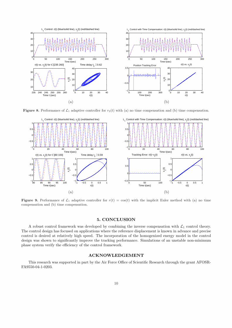
Secondly we apply the implicit Euler method to solve the ODE system (3.5) − (3.7). Using the implicitEuler method, we aim to see if it can improve the time delay problem. The simulation results for reference inputr = cos(t) are shown in Figure 9. We can see that the tracking performance is much more stable compared to theresults obtained by ODE15s (see Figure 4), but there is no significant improvement in reducing the time delay,and it takes 60% more of CPU time. Next, we apply the implicit Euler method to the same multi-frequencyreference signal that we used in section 4.1, i.e., r(t) = 2 cos(t) + 10 cos(πt/5). We note that the results, shownin Figure 10, are quite similar to the results we got by using ode15s; which means that, for this r(t), the implicitmethod doesn’t improve very much on the tracking performance, and it’s more time consuming and costly. Forthe reference signals given in Figure 6, the system responses are plotted in Figure 10 and Figure 11.

9

0 50 100 150 200 250 3000

10

20

30

40

Time t(sec)



235 240 245 250 255 260

10

20

30

Time t (sec)

r(t) vs. x1(t) for t∈ [235 260]

0 10 20 30 400

10

20

30

40

r(t)

x 1(t)


0 50 100 150 200 250 3000

10

20

30

40

Time t(sec)



0 100 200 300−1

−0.5

0

0.5

Time t(sec)


0 10 20 30 400

10

20

30

40

r(t)

x 1(t)

r(t) vs. x1(t)

(a) (b)

Figure 8. Performance of L1 adaptive controller for r2(t) with (a) no time compensation and (b) time compensation.

0 20 40 60 80 100−1

−0.5

0

0.5

1

Time t(sec)



80 85 90 95 100−1

−0.5

0

0.5

1

Time t(sec)

r(t) vs. x1(t) for t∈ [80 100]

−1 −0.5 0 0.5 1−1

−0.5

0

0.5

1

r(t)

x 1(t)


0 20 40 60 80 100−1

−0.5

0

0.5

1

Time t(sec)



0 50 100−0.5

0

0.5

1

Time t(sec)


−1 −0.5 0 0.5 1−1

−0.5

0

0.5

1

r(t)

x 1(t)

r(t) vs. x1(t)

(a) (b)

Figure 9. Performance of L1 adaptive controller for r(t) = cos(t) with the implicit Euler method with (a) no timecompensation and (b) time compensation.

5. CONCLUSION

A robust control framework was developed by combining the inverse compensation with L1 control theory.The control design has focused on applications where the reference displacement is known in advance and precisecontrol is desired at relatively high speed. The incorporation of the homogenized energy model in the controldesign was shown to significantly improve the tracking performance. Simulations of an unstable non-minimumphase system verify the efficiency of the control framework.

ACKNOWLEDGEMENT

This research was supported in part by the Air Force Office of Scientific Research through the grant AFOSR-FA9550-04-1-0203.

10

0 20 40 60 80 100−20

−10

0

10

20

Time t(sec)



70 80 90 100

−10

−5

0

5

10

Time t(sec)

r(t) vs. x1(t) for t∈ [70 100]

−20 −10 0 10 20−20

−10

0

10

20

r(t)

x 1(t)


0 20 40 60 80 100−20

−10

0

10

20

Time t(sec)



0 50 100−5

0

5

10

15

Time t(sec)


−20 −10 0 10 20−20

−10

0

10

20

r(t)

x 1(t)

r(t) vs. x1(t)

(a) (b)

Figure 10. Performance of L1 adaptive controller for r = 2 cos(t)+ 10 cos(πt/5) with the implicit Euler method with (a)no time compensation and (b) time compensation.

0 50 100 150 200 250 3000

10

20

30

40

Time t(sec)



235 240 245 250 255 26010

15

20

25

30

Time t(sec)

r(t) vs. x1(t) for t∈ [235 260]

280 285 290 295 3000

10

20

30

r(t)

x 1(t)

r(t) vs. x1(t) for t∈ [280 300]

0 50 100 150 200 250 3000

10

20

30

40

Time t(sec)



230 240 250 2600

10

20

30

40

Time t(sec)

Tracking Error: r(t)−x1(t), t∈ [20 100]

0 10 20 30 400

10

20

30

40

r(t)

x 1(t)


(a) (b)

Figure 11. Performance of L1 adaptive controller for r1(t) and r2(t) with the implicit Euler method with (a) no timecompensation and (b) time compensation.

REFERENCES1. T.R. Braun, R.C. Smith, “Efficient Implementation of Algorithms for Homogenized Energy Models”, Con-

tinuum Mechanics and Thermodynamics, 18(3-4), pp.137-155, 2006.2. C. Cao, N. Hovakimyan, “Design and Analysis of a Novel L1 Adaptive Control Architecture with Guaranteed

Transient Performance”, Proc. American Control Conference, 2006.3. C. Cao, N. Hovakimyan, “L1 Adaptive Controller for System in the Presence of Unmodelled Actuator

Dynamics”, Proc. 46th IEEE Conference on Decision and Control, 2007.4. R.C. Smith, “ Smart Material Systems: Model Development.” Philadelphia, PA: SIAM, 2005.

11

l adaptive control of hysteresis in smart materials · l1 adaptive control of hysteresis in smart...

Documents