pid control of systems with hysteresis
TRANSCRIPT
PID Control of Systems withHysteresis
by
Alex Shum
A thesispresented to the University of Waterloo
in fulfillment of thethesis requirement for the degree of
Master of Mathematicsin
Applied Mathematics
Waterloo, Ontario, Canada, 2009
c© Alex Shum 2009

I hereby declare that I am the sole author of this thesis. This is a true copy of thethesis, including any required final revisions, as accepted by my examiners.
I understand that my thesis may be made electronically available to the public.
ii

Abstract
Hysteresis is exhibited by many physical systems. Smart materials such aspiezoelectrics, magnetostrictives and shape memory alloys possess useful proper-ties, especially in the field of micropositioning, but the control of these systems isdifficult due to the presence of hysteresis. An accurate model is required to predictthe behaviour of these systems so that they can be controlled.
Several hysteresis models including the backlash, elastic-plastic and Preisachoperators are discussed in detail. Several other models are mentioned. Other con-trol methods for this problem are discussed in the form of a literature review.
The focus of this thesis is on the PID control of hysteretic systems. In particular,two systems experiencing hysteresis in their controllers are examined. The hystere-sis in each system is described by different sets of assumptions. These assumptionsare compared and found to be very similar. In the first system, a PI controller isused to track a reference signal. In the second, a PID controller is used to control asecond-order system. The stability and tracking of both systems are discussed. Anextension is made to the first system to include the dynamics of a first-order system.The results of the second system are verified to hold for a general first-order system.
Simulations were performed with the extension to a first-order system usingdifferent hysteresis models.
iii

Acknowledgements
The completion of this thesis would not have been possible without the supportfrom my family, friends, and co-workers.
Dr. Kirsten Morris has been of tremendous support throughout the entireproject, offering not only support in mathematical aspects, but also in buildingconfidence and character. Sina Valadkhan has taught me the basics and provided asolid working ground for this research topic. I’d like to also thank Dr. Brian Ingallsand Dr. Amir Khajepour for taking the time to read this work. Thanks to HelenWarren for taking care of all of the logistics. Thank you all.
I’d like to thank the wonderful community of applied mathematics graduate stu-dents and professors here at the University of Waterloo, who have been so helpfulthroughout courses and the research process. In particular: my officemate Dha-naraja Kasinathan who has had to endure all the aspects of my personality, myhousemates Antonio Sanchez, Michael Dunphy, Ben Turnbull, my research groupAmenda Chow, Rob Huneault, Matthew Cox, as well as Katie Ferguson, GregMayer, Dr. Marek Stasna, Killian Miller, Chad Wells, and Derek Steinmoeller.
To my closest friends: Inglebert Mui, Danny Li, Brandon Miles, StephanieKerrigan, Angela Gray, Lorna Yuen, Kitty Lau, Filgen Fung, Eric Hart and MarkReitsma, who’ve been there and stood by me in all aspects of life be it math-relatedor not. Thank you.
To Colin Wallace and Elizabeth Yeung at Oasis: Ray of Hope, which has pro-vided a welcome distraction to my work as well as the opportunity to serve theimpoverished here in the Kitchener-Waterloo area. Thank you for opening my eyes.
Last but certainly not least, to my Lord and Saviour Jesus Christ, throughwhich all things are made possible.
iv

Contents
List of Figures ix
1 Introduction 1
2 Hysteresis Models 3
2.1 Backlash Operator . . . . . . . . . . . . . . . . . . . . . . . . . . . 4
2.2 Elastic-Plastic Operator . . . . . . . . . . . . . . . . . . . . . . . . 7
2.3 Preisach Model . . . . . . . . . . . . . . . . . . . . . . . . . . . . . 8
2.3.1 Model Definition . . . . . . . . . . . . . . . . . . . . . . . . 8
2.3.2 Preisach Operator . . . . . . . . . . . . . . . . . . . . . . . . 9
2.3.3 Preisach Plane . . . . . . . . . . . . . . . . . . . . . . . . . 10
2.3.4 Weight Function . . . . . . . . . . . . . . . . . . . . . . . . 14
2.3.5 Physical Preisach Model . . . . . . . . . . . . . . . . . . . . 16
2.4 Other Models . . . . . . . . . . . . . . . . . . . . . . . . . . . . . . 18
2.4.1 Duhem Model . . . . . . . . . . . . . . . . . . . . . . . . . . 18
3 PID Control of Hysteretic Systems 20
3.1 Introduction . . . . . . . . . . . . . . . . . . . . . . . . . . . . . . . 20
3.1.1 PID Controllers . . . . . . . . . . . . . . . . . . . . . . . . . 20
3.1.2 Lebesgue and Hardy Spaces . . . . . . . . . . . . . . . . . . 21
3.2 PID Control of Hysteretic Systems in Literature . . . . . . . . . . . 22
3.3 Stability and Robust Position Control of Hysteretic Systems . . . . 23
3.3.1 Background and Assumptions . . . . . . . . . . . . . . . . . 23
3.3.2 Stability of the Closed-Loop System . . . . . . . . . . . . . . 26
3.3.3 Tracking . . . . . . . . . . . . . . . . . . . . . . . . . . . . . 30
3.4 Extensions to include a Linear System . . . . . . . . . . . . . . . . 33
v
3.4.1 Existence and Uniqueness . . . . . . . . . . . . . . . . . . . 34
3.4.2 Stability . . . . . . . . . . . . . . . . . . . . . . . . . . . . . 35
3.5 PID Control of Second-Order Systems with Hysteresis . . . . . . . . 38
3.5.1 Model . . . . . . . . . . . . . . . . . . . . . . . . . . . . . . 39
3.5.2 Assumptions on Hysteresis Operators . . . . . . . . . . . . . 39
3.5.3 Comparison of Assumptions from Valadkhan/Morris Paperand Logemann Papers . . . . . . . . . . . . . . . . . . . . . 42
3.5.4 Integral Control In The Presence Of Hysteresis In The Input 45
3.5.5 PID Control of Systems with Hysteresis . . . . . . . . . . . 53
3.6 Verification of Results for First-Order System . . . . . . . . . . . . 57
3.7 Other Forms of Control of Hysteretic Systems . . . . . . . . . . . . 60
3.7.1 Optimal Control . . . . . . . . . . . . . . . . . . . . . . . . 60
3.7.2 Sliding Mode Control . . . . . . . . . . . . . . . . . . . . . . 60
3.7.3 Inverse Compensation . . . . . . . . . . . . . . . . . . . . . 61
3.7.4 Adaptive Control . . . . . . . . . . . . . . . . . . . . . . . . 62
4 Simulations 63
4.1 System Description . . . . . . . . . . . . . . . . . . . . . . . . . . . 63
4.2 Implementation of Hysteresis Operators . . . . . . . . . . . . . . . . 64
4.2.1 Backlash Operator and Elastic-Plastic Operator . . . . . . . 65
4.2.2 Preisach Operator . . . . . . . . . . . . . . . . . . . . . . . . 65
4.3 Results . . . . . . . . . . . . . . . . . . . . . . . . . . . . . . . . . . 67
4.3.1 Tracking a Constant Reference Signal . . . . . . . . . . . . . 68
4.3.2 Tracking Of Other Reference Signals . . . . . . . . . . . . . 69
5 Conclusions and Future Work 74
Appendices 75
A Proofs and Details 76
A.1 Existence and Uniqueness Proof . . . . . . . . . . . . . . . . . . . . 76
A.2 Showing (3.25) satisfies Lemma A.1 . . . . . . . . . . . . . . . . . . 80
A.3 Leibniz’s Rule for Convolution Differentiation . . . . . . . . . . . . 83
A.4 Left Half Complex Plane Poles → Exponentially Decaying Functions 84
vi

B MATLAB R© Code 86
References 99
vii

List of Figures
1.1 Backlash Hysteresis [24] . . . . . . . . . . . . . . . . . . . . . . . . 2
2.1 Rate-independence . . . . . . . . . . . . . . . . . . . . . . . . . . . 5
2.2 Backlash Operator acting on u(t) = 12t sin t with h = 2, ξ = 1 . . . 6
2.3 Elastic Operator acting on u(t) = 12t sin t with h = 2, ξ = 1 . . . . . 7
2.4 Preisach Relay, [41] . . . . . . . . . . . . . . . . . . . . . . . . . . . 8
2.5 Preisach Relay while a) increasing the input u(t), b) decreasing theinput u(t) . . . . . . . . . . . . . . . . . . . . . . . . . . . . . . . . 9
2.6 Preisach Plane (Initialized) . . . . . . . . . . . . . . . . . . . . . . . 11
2.7 Left: Increasing the input to u(t) = 3, Right: Then Decreasing theinput to u(t) = −1 . . . . . . . . . . . . . . . . . . . . . . . . . . . 12
2.8 Wiping Out Property . . . . . . . . . . . . . . . . . . . . . . . . . . 13
2.9 Minor Loops within a Major Loop in a Hysteretic System, from [41] 13
2.10 An arbitrary square in a piecewise-constant weight function . . . . . 15
2.11 a) Preisach Plane in obtaining corner 1, b) The region Ω1, c) Theregion Ω2 . . . . . . . . . . . . . . . . . . . . . . . . . . . . . . . . 15
2.12 Physical Preisach Relay, see [33] . . . . . . . . . . . . . . . . . . . . 17
2.13 Left: Input, Center: Output, Right: Input-Output . . . . . . . . . . 19
3.1 (a) Clockwise Hysteresis Loop, (b) Counter-Clockwise HysteresisLoop, from [41] . . . . . . . . . . . . . . . . . . . . . . . . . . . . . 24
3.2 Closed-Loop System, from [41] . . . . . . . . . . . . . . . . . . . . . 27
3.3 Closed-Loop System defined by (3.16) - (3.19) . . . . . . . . . . . . 37
3.4 Closed-Loop System defined by equations (3.10) - (3.15) . . . . . . 38
3.5 Closed-Loop System defined by equations (3.21) and (3.22) . . . . . 39
3.6 A controlled hysteretic system with inverse compensation . . . . . . 61
4.1 MATLAB R© Preisach Plane at u = 5 (from u = 0) . . . . . . . . . . 66
viii
4.2 MATLAB R© Preisach Plane: u = [0, 7, 2.5] . . . . . . . . . . . . . . 66
4.3 Preisach Major Loop with Terfenol-D Data . . . . . . . . . . . . . . 67
4.4 Weight Function from Terfenol-D Data . . . . . . . . . . . . . . . . 68
4.5 Tracking of a Constant Reference Signal: Backlash and Elastic-Plastic, KP = 10, KI = 5, bfac = 3, efac = 3 . . . . . . . . . . . . . 69
4.6 Tracking of a Constant Reference Signal: Backlash, KP = 5, KI =10, bfac = 3 . . . . . . . . . . . . . . . . . . . . . . . . . . . . . . . 70
4.7 Tracking of a Piecewise Constant: Preisach Operator, KP = 100,KI = 10 . . . . . . . . . . . . . . . . . . . . . . . . . . . . . . . . . 70
4.8 Tracking of a Piecewise Ramp Function: Backlash and Elastic PlasticOperators, KP = 10, KI = 5 . . . . . . . . . . . . . . . . . . . . . . 71
4.9 Tracking of a Piecewise Ramp Function: Preisach Operator, KP =100, KI = 10 . . . . . . . . . . . . . . . . . . . . . . . . . . . . . . 72
4.10 Tracking of a Sinusoidal Function with Varying Amplitude: Backlashand Elastic Plastic Operators, KP = 20, KI = 10, r(t) = 0.2(5 −t) sin(0.4t) . . . . . . . . . . . . . . . . . . . . . . . . . . . . . . . . 72
4.11 Tracking of Sinusoidal Function with Varying Amplitude: PreisachOperator, KP = 100, KI = 40, r(t) = 0.05(5− t) sin(0.4t) + 0.0540 . 73
A.1 Depicting the set B(w; δ, ε) . . . . . . . . . . . . . . . . . . . . . . . 77
ix

Chapter 1
Introduction
Hysteresis is a property experienced by many materials that is highly non-linearand difficult to model. Multiple outputs can be associated with the same input,so the system may exhibit path-dependence. Hysteresis can also be described as adelay in the reaction of a material when provided with actuation. Consider mag-netic hysteresis: magnets may possess a range of magnetization values without thepresence of an applied magnetic field. It is not possible to determine magnetizationwithout knowledge of the input history.
Another example is the play behaviour exhibited by mechanical gears. In theoperation of two mated gears, turning one gear causes the other to turn. Due tothe tolerance between the teeth of each gear, the driving gear must move a certaindistance before the mated gear will move. This hysteresis is known as backlash andwill be discussed later. See Figure 1.1, obtained from [24].
An exciting group of hysteretic materials are smart materials. Relevant appli-cations are easily found in the field of micropositoning. For example, a magne-tostrictive material, Terfenol-D, can experience a change in length of 0.001m/mat a saturation magnetic field. Shape memory alloys are materials with multiplephases, in which deformed materials return to their original shape under appropri-ate temperature changes. Piezoelectric materials can convert strains into electricalsignals. The issue however, is that all of these materials possess some sort of hys-teresis. It is difficult to provide a model, and even harder to control a system thatpossesses hysteresis. For more information regarding smart materials, the reader isreferred to [32].
An attempt in this thesis is made to study the mathematics behind certainhysteretic models and their control. The majority of the work presented in thisthesis considers two closed-loop systems with hysteretic components. The controlof a hysteretic system using a PI controller and of a second-order system with a
1
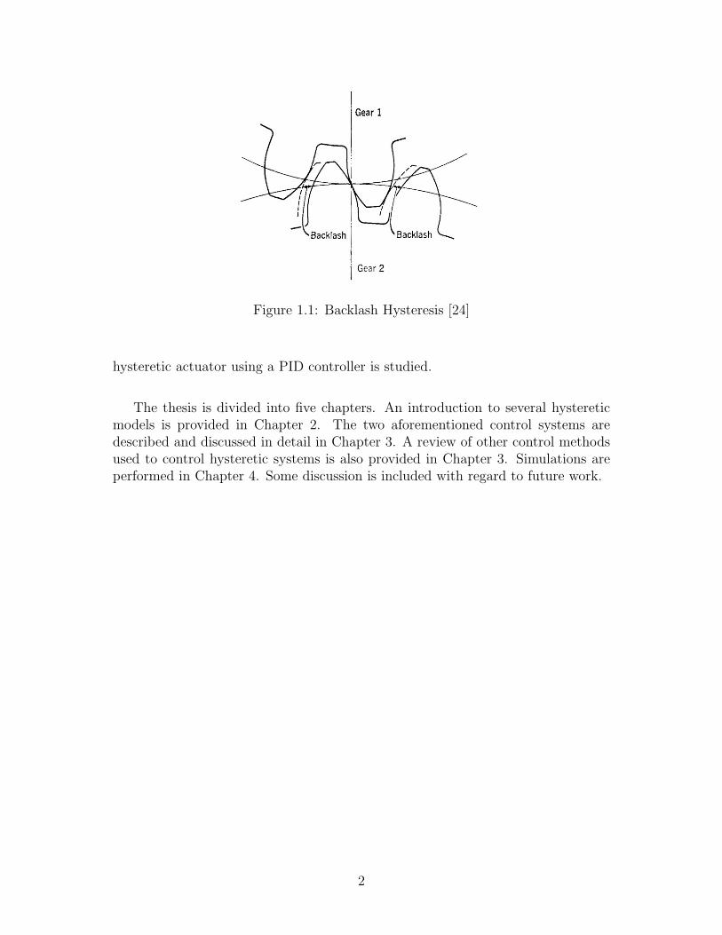
Figure 1.1: Backlash Hysteresis [24]
hysteretic actuator using a PID controller is studied.
The thesis is divided into five chapters. An introduction to several hystereticmodels is provided in Chapter 2. The two aforementioned control systems aredescribed and discussed in detail in Chapter 3. A review of other control methodsused to control hysteretic systems is also provided in Chapter 3. Simulations areperformed in Chapter 4. Some discussion is included with regard to future work.
2
Chapter 2
Hysteresis Models
As described previously, hysteresis is difficult to model due to its non-linearity, andthe need for knowledge of previous states. Considering the generality of hysteresis,it is impossible to find one model that accurately describes all types of hysteresis.Several different models that describe hysteresis will be discussed in this chapter.This small selection is meant to provide an introduction to the models studied inthe relevant research papers and theory to come.
A commonly-used mathematical definition of a hysteresis operator from [41] isfirst presented.
Let R+ := t ∈ R | t ≥ 0. Let I ⊆ R+. Let the set of all functions map-ping I to the reals be denoted by Map(I) (that is, f ∈ Map(I) ⇔ f : I → R ).The next definition is the truncation property. For T > 0, let the truncation off ∈Map(R+), be defined by
fT (t) :=
f(t), t ∈ [0, T ]
0, t > T.
Next, the two properties required to define a hysteresis operator are given. Theyare the causal and rate-independent properties. Note that in literature, the causalproperty may be also referred to as the Volterra property or the deterministicproperty.
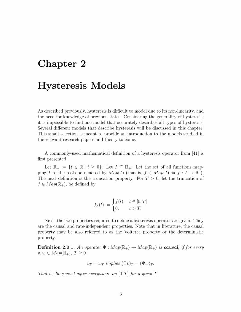
Definition 2.0.1. An operator Ψ : Map(R+) → Map(R+) is causal, if for everyv, w ∈Map(R+), T ≥ 0
vT = wT implies (Ψv)T = (Ψw)T .
That is, they must agree everywhere on [0, T ] for a given T .
3
From the definition of the causal property, the output (Ψ(v)) does not dependon future inputs, because the property must hold true for all T ≥ 0.
In order to define rate-independence, another definition must first be introduced.
Definition 2.0.2. A function f : R+ −→ R+ is a time-transformation, if f iscontinuous, nondecreasing, and lim
t→∞f(t) =∞.
Definition 2.0.3. An operator Ψ : C(R+) −→ C(R+) is rate-independent iffor all time transformations f ,
(Ψ(u f))(t) = (Ψ(u))(f(t)), for all u ∈ C(R+), for all t ∈ R+. (2.1)
That is, the order in which the operations are applied do not matter. Therate-independent operator can be applied before or after the time transformation.That is, a rate-independent operator cannot depend on derivatives of the input. Toillustrate this, a graphical example is included. See Figure 2.1.
On the left of Figure 2.1(a), the input is a sinusoidal function with varying am-plitude shown in blue, and the output of a rate-independent operator is shown ingreen. The input is plotted against the output. A piecewise linear function, con-structed with the same local maximums and minimums is in Figure 2.1(b). Notethat the input-output graphs are identical. The rate at which these local maxi-mums and minimums are reached is irrelevant to the present value. Finally, thedefinition of a hysteresis operator is presented.
Definition 2.0.4. An operator Φ : Map(R+)→ Map(R+) that is both causal andrate-independent is a hysteresis operator.
2.1 Backlash Operator
Also known as play, the backlash operator is a hysteresis operator that is used incertain mechanical applications, especially to model the play between gear trains.In terms of application, backlash is the physical clearance between mated gearteeth. The gears will turn only after a certain amount of torque is provided. Thefollowing formulation can be found in [18]. An alternative definition can be foundin [4]. A function will first be defined.
For all h ∈ R+, let the function bh : R2 → R be defined as:
4

(a) Input Signal: u(t) = 0.8t cos(πt/5)
(b) Piecewise Linear Input Signal With Same Extrema
Figure 2.1: Rate-independence
5
bh(v, w) = maxv − h,min v + h,w
The backlash operator will be defined for every h ∈ R+ and ξ ∈ R as a functionof bh. For every piecewise monotone function u ∈ C(R+),
(Bh,ξ(u))(t) =
bh(u(0), ξ), for t = 0
bh(u(t), (Bh,ξ(u))(ti))), for ti−1 < t ≤ ti, i ∈ N
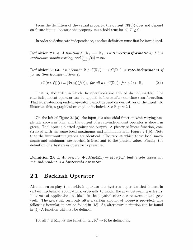
where 0 < t1 < t2 < ... is a partition of R+ such that u ∈ C(R+)→ R is monotone(only non-decreasing or only non-increasing) on each of [ti−1, ti], i ∈ N and t0 = 0.The parameter ξ represents the initial state of the operator. In the definition pro-vided above, the parameter h can be thought of as the delay in the operator fromthe input function u. This is represented visually in Figure 2.2. Using MATLAB R©,the continuous function u(t) = 1
2t sin t is plotted against the backlash operator act-
ing on this u(t), with h = 2, ξ = 1.
Figure 2.2: Backlash Operator acting on u(t) = 12t sin t with h = 2, ξ = 1
The relationship between the input u(t) and the backlash operator is shown onthe right of Figure 2.2. The operator initially starts at (1, 0). Following the plotof the u(t) given on the left, it increases and decreases without any change in theoperator. Then it proceeds to make successively larger counter-clockwise loops,closely following the shape of the input on the lines (Bh,ξ(u))(t) = u(t) + 2 and(Bh,ξ(u))(t) = u(t) − 2, which is representative of the delay of h = 2. At t = 30,the operator (in the right plot) reaches the point on the bottom left, (−15,−13).
6
2.2 Elastic-Plastic Operator
The stress and strain relationship in a one-dimensional elastic-plastic element ismodelled by this operator. If the stress applied is less than the yield stress, thenthe material’s strain can be approximated by a linear relationship (Hooke’s Law,σ = Eε, where σ is the stress, E is Young’s Modulus for the material and ε is thestrain). If the stress acting on the element becomes greater than the yield stress,then the element deforms plastically (that is,t no additional strain is observed).This mathematical definition of the elastic-plastic operator is constructed muchlike the backlash operator and can be found in [18]. Let eh : R→ R be defined by
eh(u) = minh,max−h, u,
For all h ∈ R+, for all ξ ∈ R, the elastic-plastic operator Eh,ξ is defined for piece-wise monotone functions u ∈ C(R+) by
(Eh,ξ(u))(t) =
eh(u(0)− ξ), for t = 0
eh(u(t)− u(ti) + (Eh,ξ(u))(ti))), for ti−1 < t ≤ ti, i ∈ N
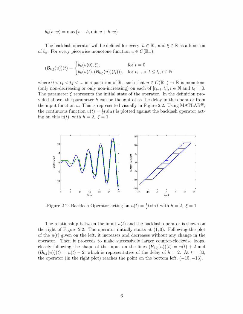
where 0 < t1 < t2 < ... is a partition of R+ such that u ∈ C(R+)→ R is monotone(only non-decreasing or only non-increasing) on each of [ti−1, ti], i ∈ N and t0 = 0.In Figure 2.3, the same function u(t) = 1
2t sin t is plotted against the elastic-plastic
operator acting on the same u(t), with h = 2, ξ = 1. Here, h represents the strainobserved once the yield stress is reached. So the operator is bounded by −h and h.The variable −ξ is the initial state of the operator.
Figure 2.3: Elastic Operator acting on u(t) = 12t sin t with h = 2, ξ = 1
The relationship between the operator and the input is shown on the right ofFigure 2.3. As mentioned previously, the property |(Eh,ξ(u))(t)| ≤ h is satisfied
7
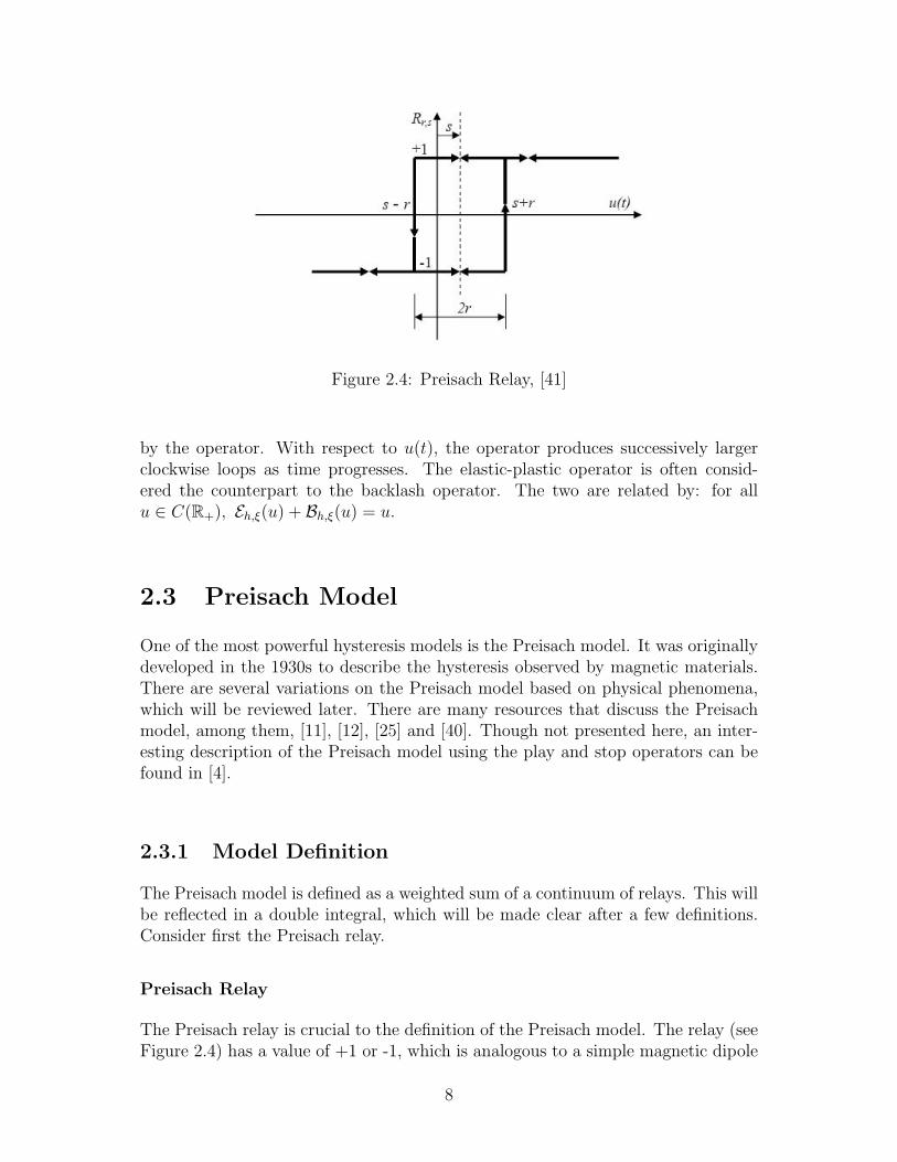
Figure 2.4: Preisach Relay, [41]
by the operator. With respect to u(t), the operator produces successively largerclockwise loops as time progresses. The elastic-plastic operator is often consid-ered the counterpart to the backlash operator. The two are related by: for allu ∈ C(R+), Eh,ξ(u) + Bh,ξ(u) = u.
2.3 Preisach Model
One of the most powerful hysteresis models is the Preisach model. It was originallydeveloped in the 1930s to describe the hysteresis observed by magnetic materials.There are several variations on the Preisach model based on physical phenomena,which will be reviewed later. There are many resources that discuss the Preisachmodel, among them, [11], [12], [25] and [40]. Though not presented here, an inter-esting description of the Preisach model using the play and stop operators can befound in [4].
2.3.1 Model Definition
The Preisach model is defined as a weighted sum of a continuum of relays. This willbe reflected in a double integral, which will be made clear after a few definitions.Consider first the Preisach relay.
Preisach Relay
The Preisach relay is crucial to the definition of the Preisach model. The relay (seeFigure 2.4) has a value of +1 or -1, which is analogous to a simple magnetic dipole
8

Figure 2.5: Preisach Relay while a) increasing the input u(t), b) decreasing theinput u(t)
that can only take on a value of ±1. The relay has two parameters: r and s. Thecentre of the relay is denoted by s, while the half-width of the relay is denoted byr. Physically, r can be thought of as the resistance towards switching and s is thecritical magnetization where switching can occur. Finally, to determine the outputof the relay, a history of the relay is required. To illustrate this, suppose the inputu(t), lies between s− r and s + r. According to Figure 2.4, there are two possibleoutputs for the relay.
Consider Figure 2.5. Following the left figure, suppose u(t) < s− r. Since thereis only one input, the relay has a value of -1. In order for the relay to switch, u(t)must be increased past s + r for the relay to switch to +1. Analogously, on theright, suppose u(t) > s+ r, then u(t) must be decreased past s− r for the relay toswitch to -1. To resolve the previous dilemma, if u(t) lies between s− r and s+ r,then the relay takes on the value of the most recent output. Finally, each pair ofparameters (r, s) (note r must be nonnegative since it represents a half-width) hasa one-to-one correspondence with a specific relay. With this definition in place, theactual model can now be introduced. The issue of initial states will be dealt within the following section.
2.3.2 Preisach Operator
The Preisach operator is described as follows,
y(t) =
∫ ∞0
∫ ∞−∞
Rr,s(u(t))µ(r, s)dsdr, (2.2)
where Rr,s is the relay with centre s and half width r, u(t) is the input, µ(r, s) isthe weight function and y(t) is the output of the model. The weight function must
9
be integrable, that is, y(t) in equation (2.2) must always be finite. This is remi-niscent of an induced magnetic field (input) producing a magnetization (output)on a magnet. At first glance, there appears to be a difficulty in implementationdue to the infinite double integral. Storage of all the history appears impossible.Furthermore, measuring a continuum of relays would raise issues with computation.However, several simplifications can be made, which lead to simpler computation.
2.3.3 Preisach Plane
The first of these simplifications is based upon physical systems having limitations.The system is assumed to exhibit saturation in the presence of a large enough in-put. As well, it is clear that in any physical computation, the integral cannot beevaluated exactly, so an approximation of a finite sum of selected relay outputs isconsidered instead.
The Preisach plane is a two-dimensional graphical construction with r on thex-axis, and s on the y-axis. Each point represents a potential relay (with r and s tobe the parameters of the relay). Since r represents the half-width, which must bepositive, the discussion is limited to points/relays on the right half of the Preisachplane. Next, only relays that have the capability of switching will be considered.Referring back to the Preisach Relay (see Figure 2.4), note that s − r and s + rare the switching points for a given relay with parameters r and s. Therefore onlyrelays that satisfy −usat ≤ s− r ≤ s + r ≤ usat are of interest. Note that this haseffectively changed the bounds from being infinite to finite.
The next statements deal with the initial state of the Preisach Plane. If thesystem is initialized (prior to any input), then relays with s > 0 and s < 0 will beassumed to have values of −1 and +1 respectively. If s = 0, then the relay willremain at 0 until the input causes the relay to switch (increased past s−r or s+r).All of these assumptions result in the Preisach plane in Figure 2.6. As a side note,other sources of literature (for example [36] and [17]) define the Preisach plane sothat the end result is a 135 degree counter-clockwise rotation of the descriptionseen here. This is merely a change of coordinates and the two forms are otherwiseidentical.
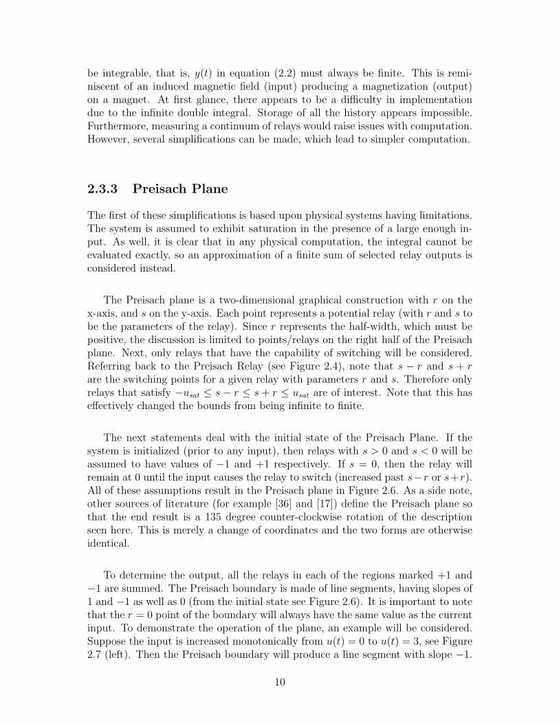
To determine the output, all the relays in each of the regions marked +1 and−1 are summed. The Preisach boundary is made of line segments, having slopes of1 and −1 as well as 0 (from the initial state see Figure 2.6). It is important to notethat the r = 0 point of the boundary will always have the same value as the currentinput. To demonstrate the operation of the plane, an example will be considered.Suppose the input is increased monotonically from u(t) = 0 to u(t) = 3, see Figure2.7 (left). Then the Preisach boundary will produce a line segment with slope −1.
10

Figure 2.6: Preisach Plane (Initialized)
This is consistent with the previous definitions, since the line segment produced isin fact s + r = 3, indicating that all the relays s + r ≤ 3 have switched to the +1state. Suppose the input is now decreased monotonically to u(t) = −1, then theresult is another line segment of slope +1, described by s − r = 1. In Figure 2.7(right), the relays with both s + r ≤ 3 and s − r ≥ 1 have switched back to anoutput of −1. Note that the Preisach boundary has a corner, indicating that theinput was once at u(t) = 3, (but now is at u(t) = −1). Further non-monotonicchanges in the input would result in different corners in the Preisach boundary. Itis clear that the Preisach boundary contains information regarding the history ofthe input. The next property regarding the Preisach plane will demonstrate this.
Continuing the previous example, suppose that the input is now increased mono-tonically from u(t) = −1 to u(t) = 4. As u(t) increases, a new line segment with −1slope will be introduced, hence introducing a corner indicating that the input wasonce at u(t) = −1 (See Figure 2.8 (left)). But as the input increases past u(t) = 3,both these corners will be wiped out, yielding only a single line segment of slope−1. At u(t) = 4, there will be only a single line segment: s+ r = 4 (See Figure 2.8(right)). That is, the Preisach boundary only retains information about the mostrecent extrema. If the input is increased or decreased past previous extrema, thenthat part of the memory is wiped out. Not surprisingly, this is known as the wipingout property. With regard to computation, an alternative definition can be madethat uses the Presiach boundary ψ(t, r) at time t. Consider
11
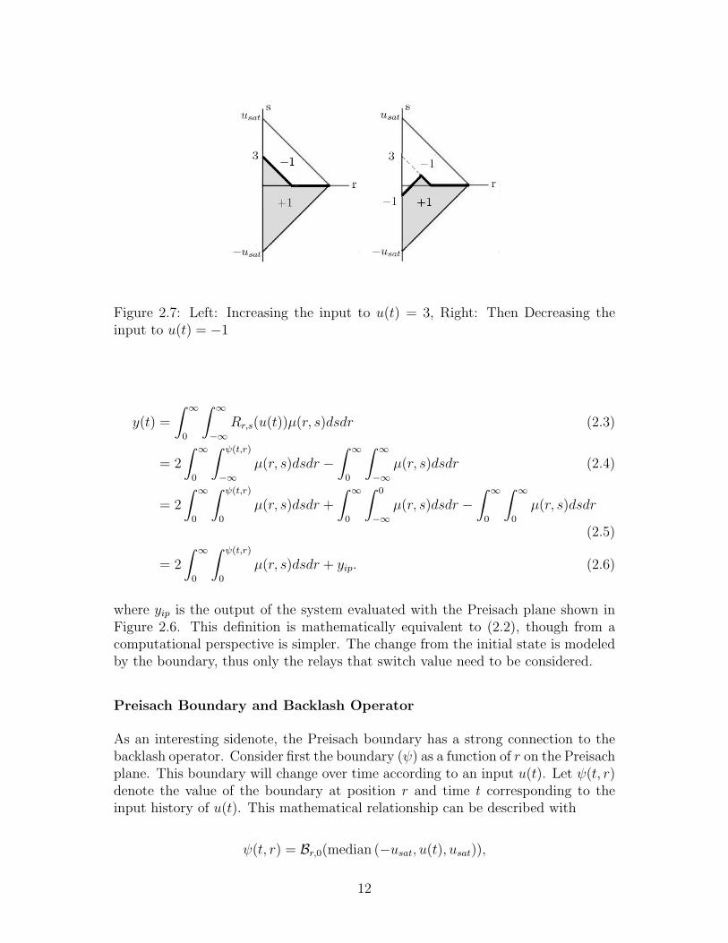
Figure 2.7: Left: Increasing the input to u(t) = 3, Right: Then Decreasing theinput to u(t) = −1
y(t) =
∫ ∞0
∫ ∞−∞
Rr,s(u(t))µ(r, s)dsdr (2.3)
= 2
∫ ∞0
∫ ψ(t,r)
−∞µ(r, s)dsdr −
∫ ∞0
∫ ∞−∞
µ(r, s)dsdr (2.4)
= 2
∫ ∞0
∫ ψ(t,r)
0
µ(r, s)dsdr +
∫ ∞0
∫ 0
−∞µ(r, s)dsdr −
∫ ∞0
∫ ∞0
µ(r, s)dsdr
(2.5)
= 2
∫ ∞0
∫ ψ(t,r)
0
µ(r, s)dsdr + yip. (2.6)
where yip is the output of the system evaluated with the Preisach plane shown inFigure 2.6. This definition is mathematically equivalent to (2.2), though from acomputational perspective is simpler. The change from the initial state is modeledby the boundary, thus only the relays that switch value need to be considered.
Preisach Boundary and Backlash Operator
As an interesting sidenote, the Preisach boundary has a strong connection to thebacklash operator. Consider first the boundary (ψ) as a function of r on the Preisachplane. This boundary will change over time according to an input u(t). Let ψ(t, r)denote the value of the boundary at position r and time t corresponding to theinput history of u(t). This mathematical relationship can be described with
ψ(t, r) = Br,0(median (−usat, u(t), usat)),
12
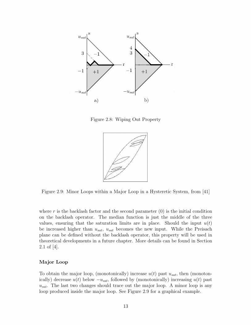
Figure 2.8: Wiping Out Property
Figure 2.9: Minor Loops within a Major Loop in a Hysteretic System, from [41]
where r is the backlash factor and the second parameter (0) is the initial conditionon the backlash operator. The median function is just the middle of the threevalues, ensuring that the saturation limits are in place. Should the input u(t)be increased higher than usat, usat becomes the new input. While the Preisachplane can be defined without the backlash operator, this property will be used intheoretical developments in a future chapter. More details can be found in Section2.1 of [4].
Major Loop
To obtain the major loop, (monotonically) increase u(t) past usat, then (monoton-ically) decrease u(t) below −usat, followed by (monotonically) increasing u(t) pastusat. The last two changes should trace out the major loop. A minor loop is anyloop produced inside the major loop. See Figure 2.9 for a graphical example.
13
2.3.4 Weight Function
It remains to discuss how the weight function is identified. There are several ap-proaches to this problem. A general form of the weight function can be assumed(for example, see Section 2.3.5), with varying parameters to be found through opti-mization of error in comparison to experimental data. Optimization may not yielda good result if an inappropriate shape is chosen. A popular choice for identifyingthe weight function is to discretize the Preisach plane into squares of equal sizewhere the weight function is assumed to be constant over each square region. Inliterature, this process is referred to performing a discretization of level L, whereL represents the number of squares along the centre. Thus the whole Preisachplane would have L2 components. Assuming a proper identification technique isused for each square, the higher the level of discretization L, the better the accuracy.
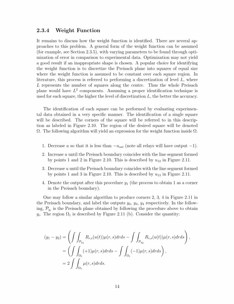
The identification of each square can be performed by evaluating experimen-tal data obtained in a very specific manner. The identification of a single squarewill be described. The corners of the square will be referred to in this descrip-tion as labeled in Figure 2.10. The region of the desired square will be denotedΩ. The following algorithm will yield an expression for the weight function inside Ω.
1. Decrease u so that it is less than −usat (note all relays will have output −1).
2. Increase u until the Preisach boundary coincides with the line segment formedby points 1 and 2 in Figure 2.10. This is described by u12 in Figure 2.11.
3. Decrease u until the Preisach boundary coincides with the line segment formedby points 1 and 3 in Figure 2.10. This is described by u13 in Figure 2.11.
4. Denote the output after this procedure y1 (the process to obtain 1 as a cornerin the Preisach boundary).
One may follow a similar algorithm to produce corners 2, 3, 4 in Figure 2.11 inthe Preisach boundary, and label the outputs y2, y3, y4 respectively. In the follow-ing, Pyi is the Preisach plane obtained by following the procedure above to obtainyi. The region Ω1 is described by Figure 2.11 (b). Consider the quantity:
(y1 − y2) =
(∫ ∫Py1
Rr,s(u(t))µ(r, s)drds−∫ ∫
Py2Rr,s(u(t))µ(r, s)drds
),
=
(∫ ∫Ω1
(+1)µ(r, s)drds−∫ ∫
Ω1
(−1)µ(r, s)drds
),
= 2
∫ ∫Ω1
µ(r, s)drds.
14
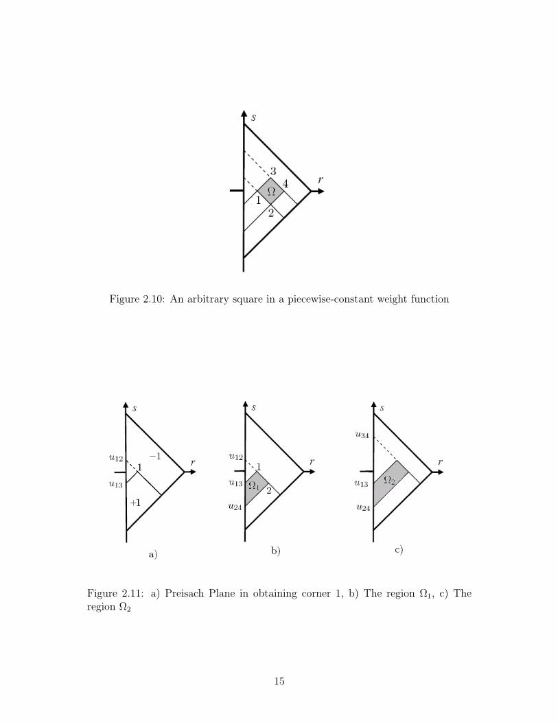
Figure 2.10: An arbitrary square in a piecewise-constant weight function
Figure 2.11: a) Preisach Plane in obtaining corner 1, b) The region Ω1, c) Theregion Ω2
15
It is easy to see that a similar region (but one that includes the square of interest)can be produced by considering the quantity (y3 − y4). Denote this region Ω2 (seeFigure 2.11 c)). Then the following expression will result in a weight function forthe square of interest. The side length of the square will be denoted c. The valueµΩ is the constant value of the weight function in the region Ω.
1
2c2((y3 − y4)− (y1 − y2)) =
1
2c2
(2
∫ ∫Ω2
µ(r, s)drds− 2
∫ ∫Ω1
µ(r, s)drds
),
=1
c2
∫ ∫Ω
µ(r, s)drds,
=1
c2µΩ
∫ ∫Ω
drds,
= µΩ.
The second last step is a result of the weight function assumed constant overthis region. The experimental data used to identify the weight function is a set offirst-order descending curves. For a discretization of level L (L ∈ N), L + 1 first-order descending curves are required. Suppose the range of the outputs in the majorloop is divided into L equally spaced intervals (resulting in L + 1 equally spacedpoints). Then the ith curve (i ∈ 1, 2, ..., L+ 1) is obtained by decreasing the inputu(t) below −usat (so that all the relays are in the −1 state, then increasing the in-put monotonically to the ith point, followed by decreasing the input monotonicallyback to −usat. This is very similar to the procedure outlined above to obtain thesquare region Ω. The differences are that the procedure is performed L + 1 times(once for each curve), and in the third step, u(t) is decreased monotonically backdown to −usat, while sampling at each potential square corner. This approach isattractive because it is simple both experimentally and computationally.
2.3.5 Physical Preisach Model
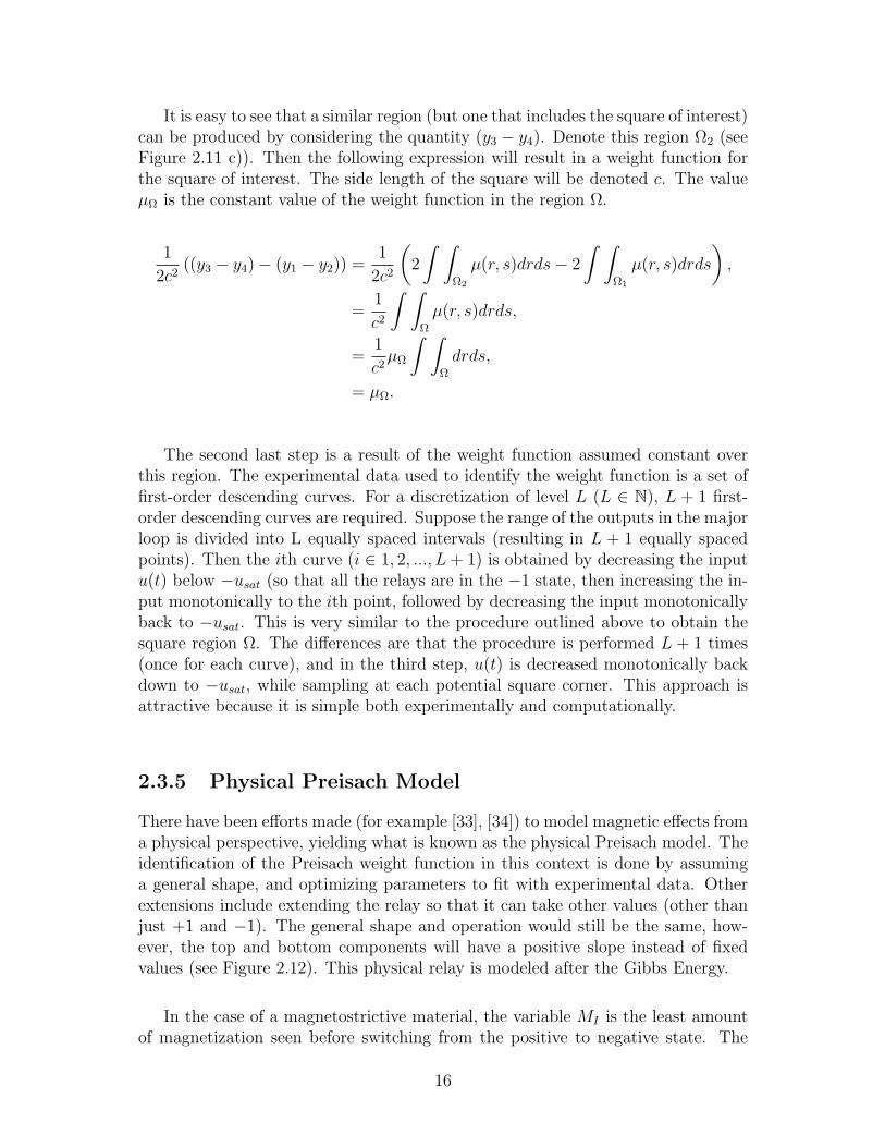
There have been efforts made (for example [33], [34]) to model magnetic effects froma physical perspective, yielding what is known as the physical Preisach model. Theidentification of the Preisach weight function in this context is done by assuminga general shape, and optimizing parameters to fit with experimental data. Otherextensions include extending the relay so that it can take other values (other thanjust +1 and −1). The general shape and operation would still be the same, how-ever, the top and bottom components will have a positive slope instead of fixedvalues (see Figure 2.12). This physical relay is modeled after the Gibbs Energy.
In the case of a magnetostrictive material, the variable MI is the least amountof magnetization seen before switching from the positive to negative state. The
16
Figure 2.12: Physical Preisach Relay, see [33]
value MR is the magnetization observed when the applied magnetic field is 0. Thelocal magnetization is denoted by M , representing the amount of magnetization ofthat specific dipole. The coercive field HC , or switching point, is the same as r+ sin the phenomenological model. The interaction field, HI plays the same role as s.Instead of different centre locations, the same definition, but with an offset of HI isused. Finally H is the applied magnetic field. For a visual representation of thesevalues with the Gibbs energy, the reader is referred to Section 2 of [33].
With this different formulation, the model equation itself becomes
M(H) =
∫ ∞0
∫ ∞−∞
ν1(Hc)ν2(HI)M(H +HI ;Hc; ξ)dHIdHC . (2.7)
where ξ represents the last known position (whether it is on the positive or negativepart of the relay). The weight function components ν1 and ν2 in [33] are given by
ν1(Hc) =c1
I1
e−[ln(Hc/HC)/2c]2 ,
ν2(HI) = c2e−H2
I /2b2
,
I1 =
∫ ∞0
ν1(Hc)dHC .
where c1, c2, and b are positive real parameters obtained through optimization inaccordance to provided data. These are not the only choices for the weight function.There are however some general criteria that should be followed. Both functionsshould follow certain decay properties. The function ν2 should be even. Extensionshave been made in [42] and [33] to include the effects of compressive loads on thehysteresis of magnetostrictives.
The definition of three operators have been provided, but it should be mentionedthat they are in fact hysteresis operators as described by Definition 2.0.4. Recall
17
that hysteresis operators must be both causal and rate-independent. The backlash,elastic-plastic and Preisach operators satisfy this definition. It is clear that theyare causal. Rate-independence for each operator follows with a simple substitutionverifying that the equality in equation (2.1) holds.
2.4 Other Models
There are many more hysteresis models that have not been discussed. The hystere-sis models discussed thus far are described by operators acting on functions. Thefollowing hysteresis model is described by systems of differential equations. TheDuhem model is a very general model that has a purely mathematical basis. Othermodels can be easily found in literature. The reader is referred to [32] for moregeneral models regarding hysteresis. For specifics to magnetic and magnetostrictivematerials, a wide variety of hysteresis models can be fonud in [39] and [40].
2.4.1 Duhem Model
The Duhem model was developed at the end of the last century by a French math-ematician Pierre Duhem [4]. The model is used widely to model friction, and theMaxwell-slip model is a special case of the Duhem model [29]. Only the previousstep of the input in terms of memory is required to determine whether is increasing,decreasing or stationary. The definition takes the form of a differential equation:
w′(t) = f+(t, v, w)(v′(t))+ − f−(t, v, w)(v′(t))−, w(0) = w0.
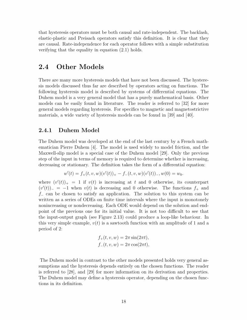
where (v′(t))+ = 1 if v(t) is increasing at t and 0 otherwise, its counterpart(v′(t))− = −1 when v(t) is decreasing and 0 otherwise. The functions f+ andf− can be chosen to satisfy an application. The solution to this system can bewritten as a series of ODEs on finite time intervals where the input is monotonelynonincreasing or nondecreasing. Each ODE would depend on the solution and end-point of the previous one for its initial value. It is not too difficult to see thatthe input-output graph (see Figure 2.13) could produce a loop-like behaviour. Inthis very simple example, v(t) is a sawtooth function with an amplitude of 1 and aperiod of 2:
f+(t, v, w) = 2π sin(2πt),
f−(t, v, w) = 2π cos(2πt),
The Duhem model in contrast to the other models presented holds very general as-sumptions and the hysteresis depends entirely on the chosen functions. The readeris referred to [28], and [29] for more information on its derivation and properties.The Duhem model may define a hysteresis operator, depending on the chosen func-tions in its definition.
18

Figure 2.13: Left: Input, Center: Output, Right: Input-Output
19

Chapter 3
PID Control of HystereticSystems
3.1 Introduction
PID control is a well understood branch of control theory. In this chapter, twogroups of hysteretic systems will be controlled by PID controllers in order to tracka constant reference signal. A brief introduction to PID controllers and literaturereview is presented in the following section. In [41], a system experiencing hys-teresis is controlled with a PI controller. These mathematical results are presentedin Section 3.3. An extension is made in Section 3.4 to include a linear first-ordersystem and some similar properties and results are shown.
In [18], a second-order system experiencing hysteresis in the actuator is con-trolled to track a constant reference signal. These results are discussed in Section3.5. A verification is presented in Section 3.6 that the same results hold for a gen-eral first order system. The assumptions of [18] and [41] are compared in Section3.5.3. Finally, a literature survey discussing other popular methods of control inthe context of hysteresis systems is presented.
3.1.1 PID Controllers
PID controllers are commonly used in feedback control. The goal of the controlleris to steer the system to follow a given reference signal. The error is defined as thedifference between the output and a reference signal. Proportional, integral andderivative components of the error can be found in the PID Controller. For thefollowing controller, KP , KI , KD > 0 are the proportional, integral and derivativecontrol parameters respectively. The general form of the PID controller is:
u(t) = KP e(t) +KI
∫ t
0
e(τ)dτ +KDe′(t). (3.1)
20
The Laplace transform of a function f ∈ C(R+) is
(Lf(t))(s) = f(s) =
∫ ∞0
f(t)e−stdt.
It is convenient to write the PID controller and other linear transformationsin terms of a transfer function. A transfer function is a representation of a linearoperator in the Laplace domain, defined by the Laplace transform of the outputdivided by the Laplace transform of the input. For the PID controller describedabove, if e(0) = 0,
u(s)
e(s)= KP +
KI
s+KDs.
Proportional control changes the controller by an amount that is proportionalto the error. The system can become unstable if the value of KP is too high. Con-versely, if KP is too low, then the controller may not be responsive to large errors.Integral control considers previous values of error, and adjusts the input accord-ingly. A larger value of KI will eliminate steady-state error faster but may causeovershoot (the state moves past the reference signal and then returns to stabilize).Derivative control affects the controller by considering the derivative of the error.Applying derivative control reduces the rate of change of the controller, and hencethe overshoot is decreased. The derivative control is sensitive to noise. The deriva-tive of the noise is usually unbonuded. More information regarding PID controllerscan be found in [26].
3.1.2 Lebesgue and Hardy Spaces
The notion of Lebesgue and Hardy spaces will be used throughout the chapter.More information can be found in [8] and [9]. The space of Lp(R+) functions willnow be introduced.
Lebesgue Spaces: Lp(R+)
For 1 ≤ p <∞ and a function f
‖f‖p =
(∫ ∞0
|f(t)|pdt) 1
p
.
21
In the case of p =∞,
‖f‖∞ = supt∈R+
|f(t)|.
A function f belongs to an Lp(R+) space if its Lp(R+)-norm is finite. Next, theset of functions that are locally Lp(R+) where p ∈ N
⋃∞) will be introduced.
Recall the truncation property defined earlier in the beginning of Chapter 2. Afunction f ∈ Lploc if for every T > 0,
‖fT‖P <∞.
Hardy Spaces: H2(C+) and H∞(C+)
The results in this chapter require the definition of two Hardy spaces. A morespecific version of the definition found in [8, Definition A.6.14] is presented here.
Definition 3.1.1. A complex-valued function f ∈ H2(C+) if it is holomorphic onthe right-half complex plane and
‖f‖2H2 := sup
x>0
(1
2π
∫ ∞−∞‖f(x+ iy)‖2 dy
)<∞. (3.2)
Definition 3.1.2. A complex-valued function f ∈ H∞(C+) if it is holomorphic onthe right-half complex plane and
‖f‖H∞ := supRe(s)>0
|f(s)| = supω∈R|f(iw)| <∞. (3.3)
3.2 PID Control of Hysteretic Systems in Liter-
ature
Before the main work is presented, a brief overview of other PID-related workavailable in the literature regarding stability of controlled hysteretic systems will bementioned. Each of the hysteresis models are described in their respective papers.In [16], a second-order system with hysteretic effects in the spring term, modeledby the Bouc-Wen model, is controlled using a PID controller. The Bouc-Wenmodel is a specific case of a rate-independent Duhem model. The closed loopsignals are shown to satisfy boundedness, and the Routh-Hurwitz criterion is usedto demonstrate asymptotic stability of the error. A similar study can be foundin [18] (expanded further in [22]), where the effects and control of a hystereticspring is considered. The hysteresis operator is formulated in the same manner asin Section 3.5.2. Experimental data is presented in both works. A PID controllercombined with inverse compensation (discussed in Section 3.7.3) approach where
22
the constants are determined experimentally is used in [14]. Shape memory alloyactuators represented by a Preisach model are controlled in [1] with use of fuzzylogic components and a PID controller. Lyapunov methods are used to demonstratestability. Finally, in [5], a PID controller is used alongside a feedback linearizationloop and repetitive controller on a system exhibiting Maxwell slip model hysteresis.Stability is obtained with a small gain theorem.
3.3 Stability and Robust Position Control of Hys-
teretic Systems
The position control of a hysteretic system using a PI controller is discussed in [41].For arbitrary reference signals, the closed-loop system is shown to be BIBO-stablewith a gain of one. In the case of a constant reference signal, zero-state error andmonotonically decreasing error are guaranteed. A bound on the time to reach anarbitrarily small error is found. All the material in this section can be found in [4]and [41].
3.3.1 Background and Assumptions
Several sets that deal with extensions of existing functions are defined. These setswill be useful in the context of proving existence and uniqueness of solutions infuture sections. For every δ > 0, 0 ≤ t1 ≤ t2, w ∈ C([0, t1]), let
B1(w, t1, t2) := u ∈ C([0, t2]) | ut1 = wt1.
The set B1 is the set of all continuous extensions of w from t1 to t2.
Some assumptions on the hysteresis operator (Definition 2.0.4) are required andwill be applied throughout the next few theorems. In the following assumptions,y(t) = Φ(u(t)), where Φ is a hysteresis operator.
(A1) If u(t) is continuous, then y(t) is continuous.
(A2) There exists λ > 0, such that for all 0 ≤ t1 ≤ t2, w ∈ C([0, t1]), u1, u2 ∈B1(w, t1, t2),
supt1≤τ≤t2
|Φ(u1)(τ)− Φ(u2)(τ)| ≤ λ supt1≤τ≤t2
|u1(τ)− u2(τ)|
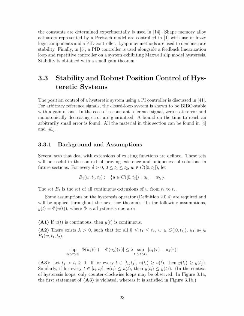
(A3): Let tf > ti ≥ 0. If for every t ∈ [ti, tf ], u(ti) ≥ u(t), then y(ti) ≥ y(tf ).Similarly, if for every t ∈ [ti, tf ], u(ti) ≤ u(t), then y(ti) ≤ y(tf ). (In the contextof hysteresis loops, only counter-clockwise loops may be observed. In Figure 3.1a,the first statement of (A3) is violated, whereas it is satisfied in Figure 3.1b.)
23
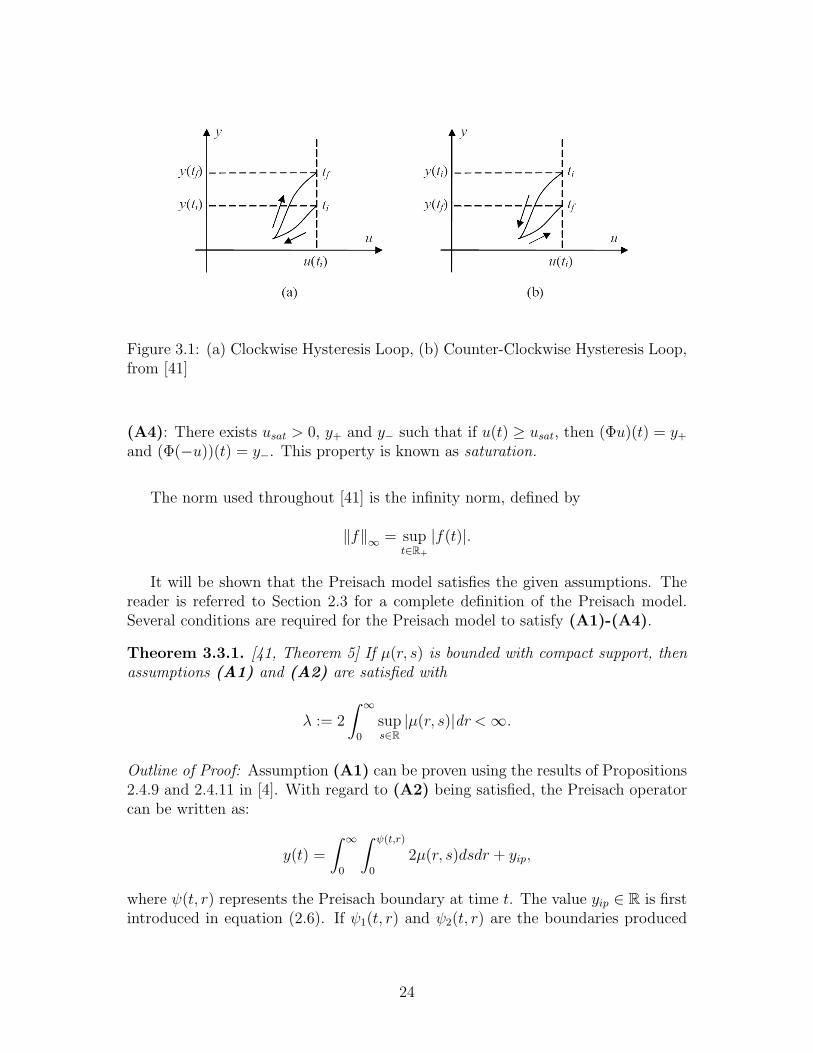
Figure 3.1: (a) Clockwise Hysteresis Loop, (b) Counter-Clockwise Hysteresis Loop,from [41]
(A4): There exists usat > 0, y+ and y− such that if u(t) ≥ usat, then (Φu)(t) = y+
and (Φ(−u))(t) = y−. This property is known as saturation.
The norm used throughout [41] is the infinity norm, defined by
‖f‖∞ = supt∈R+
|f(t)|.
It will be shown that the Preisach model satisfies the given assumptions. Thereader is referred to Section 2.3 for a complete definition of the Preisach model.Several conditions are required for the Preisach model to satisfy (A1)-(A4).
Theorem 3.3.1. [41, Theorem 5] If µ(r, s) is bounded with compact support, thenassumptions (A1) and (A2) are satisfied with
λ := 2
∫ ∞0
sups∈R|µ(r, s)|dr <∞.
Outline of Proof: Assumption (A1) can be proven using the results of Propositions2.4.9 and 2.4.11 in [4]. With regard to (A2) being satisfied, the Preisach operatorcan be written as:
y(t) =
∫ ∞0
∫ ψ(t,r)
0
2µ(r, s)dsdr + yip,
where ψ(t, r) represents the Preisach boundary at time t. The value yip ∈ R is firstintroduced in equation (2.6). If ψ1(t, r) and ψ2(t, r) are the boundaries produced
24
by input histories u1(t) and u2(t), respectively at time t, then
|y1(t)− y2(t)| =
∣∣∣∣∣∫ ∞
0
∫ ψ1(t,r)
0
2µ(r, s)dsdr −∫ ∞
0
∫ ψ2(t,r)
0
2µ(r, s)dsdr
∣∣∣∣∣ ,=
∣∣∣∣∣∫ ∞
0
∫ ψ1(t,r)
ψ2(t,r)
2µ(r, s)dsdr
∣∣∣∣∣ ,≤ 2
∫ ∞0
sups∈R
µ(r, s)dr ‖ψ1(t)− ψ2(t)‖∞ ,
≤ 2
∫ ∞0
sups∈R
µ(r, s)dr ‖u1 − u2‖∞ .
A detailed proof of the last two lines is provided in Lemmas 2.3.2 and 2.4.8 in [4].
Theorem 3.3.2. [41, Theorem 6] If µ(r, s) ≥ 0 for every r, s, (A3) holds.
Proof. Let tf > ti ≥ 0. Suppose u is such that for every t ∈ [ti, tf ], u(t) ≤ u(ti).Comparing the state of the system at tf and ti, let Ω+ denote the set of relays thatswitched from −1 to +1 and let Ω− be the set of relays that switched from −1 to +1.
y(tf )− y(ti) =
∫∫Ω+
(+1)µ(r, s)drds +
∫∫Ω−
(−1)µ(r, s)drds
−[∫∫
Ω+
(−1)µ(r, s)drds +
∫∫Ω−
(+1)µ(r, s)drds
]= 2
∫∫Ω+
µ(r, s)drds− 2
∫∫Ω−
µ(r, s)drds
Since u(t) ≤ u(ti) for every t ∈ [ti, tf ], no relays could have switched from −1 to+1. Hence the set Ω+ is empty. This, together with the property that µ(r, s) ≥ 0for all r, s, implies that
y(tf )− y(ti) = −2
∫∫Ω−
µ(r, s)drds ≤ 0.
Therefore y(tf ) ≤ y(ti), as required. For the second statement, with the as-sumption that u(t) ≥ u(ti), the set Ω− can be shown to be empty by an analogousargument, so y(tf ) ≥ y(ti) as required.
Finally, the Preisach model will be shown to satisfy (A4).
Theorem 3.3.3. [41, Theorem 7] Assume there is usat > 0 such that µ(r, s) = 0for |r + s| or |r − s| larger than usat > 0, and define
y+ =
∫ ∞−∞
∫ ∞0
µ(r, s)drds
y− =
∫ ∞−∞
∫ ∞0
−µ(r, s)drds.
25
If u(t) ≥ usat or u(t) ≤ −usat, then y(t) is equal to y+ or y− respectively, satisfying(A4).
Proof. Let u(t) ≥ usat. If the switching point, r + s (refer to Figure 2.4) of a relayis past usat, its weight must be 0. All the relays that correspond to when µ 6= 0are in the +1 state. By applying the definition of y, if u(t) ≥ usat, then y(t) = y+.The analagous argument is true, if u(t) ≤ −usat, then y(t) = y−.
The Preisach model has been shown to satisfy assumptions (A1) - (A4) pro-vided that reasonable assumptions on µ are satisfied. In particular, (A1) - (A4)hold if the weight function µ, is both nonnegative and has compact support. Inthe context of physical systems, the weight function at a point represents the con-tribution of the relays with a specific configuration. This value must intuitivelybe nonnegative. The notion of a weight function having compact support assumesthat relays that require extensive actuation do not have a considerable impact onthe output. If the contribution coming from relays that require large actuation issignificant, then usat can be increased accordingly. An infinite amount of actuationis not realistic for a physical system, so a suitable usat can be chosen.
3.3.2 Stability of the Closed-Loop System
It will be shown that the controlled hysteretic system described below is BIBO(Bounded Input Bounded Output)-stable.
Definition 3.3.4. Let an operator R : C(I) → C(I). R is BIBO-stable if forevery u ∈ C(I), Ru ∈ C(I), and there exists ρ such that:
||(Ru)||∞ ≤ ρ||u||∞.
The smallest such ρ is known as the gain.
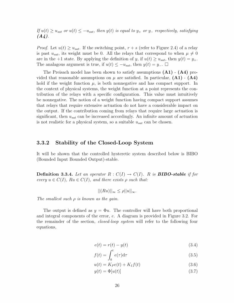
The output is defined as y = Φu. The controller will have both proportionaland integral components of the error, e. A diagram is provided in Figure 3.2. Forthe remainder of the section, closed-loop system will refer to the following fourequations,
e(t) = r(t)− y(t) (3.4)
f(t) =
∫ t
0
e(τ)dτ (3.5)
u(t) = KP e(t) +KIf(t) (3.6)
y(t) = Φ[u(t)] (3.7)
26

Figure 3.2: Closed-Loop System, from [41]
The transfer function of the controller, C is C(s) =u(s)
e(s)= KP +
KI
s, where
KI and KP are chosen control parameters. With regard to the system parameters,the following two assumptions are required.
(B1) 0 ≤ KPλ < 1, and KI > 0, where λ > 0 is the Lipschitz constant describedin (A2).
(B2) The reference signal, r(t) is continuous (that is, r(t) ∈ C(R+)).
Theorem 3.3.5. [41, Theorem 4] If Φ is a hysteresis operator, and satisfies (A3)and (A4), then y− ≤ y(t) ≤ y+ for every t.
Proof. If |u(t)| > usat, assumption (A4) implies that y ∈ y+, y−. Otherwise,let u(ti) and y(ti) be the input and output of the system at an arbitrary time ti.If u(ti) ≤ usat, monotonically increase u to u(tf ) > usat (where tf > ti). From(A3), y(ti) ≤ y(tf ), and from the saturation property in (A4), y(tf ) = y+, andhence y(ti) ≤ y+. An opposite argument with a monotone decrease will result iny(ti) ≥ y−. Since ti was chosen arbitrarily, this holds for all possible t.
The next lemma will demonstrate the existence and uniqueness of the solutionto the closed-loop system on a small interval.
Lemma 3.3.6. [41, Lemma 9] Assume (A1), (A2), (B1), (B2) are satisfied.For every t0 ≥ 0 such that the closed-loop system has a unique solution, u on [0, t0],the closed-loop system will have a unique solution u on C([t0, t0 + t)), where
t =1−KPλ
2λKI
.
Proof. Let x ∈ C([0, t0]). Define the operator
(Gx)(t) = KI
∫ t
0
(r(τ)− (Φx)(τ))dτ +KP (r(t)− (Φx)(t)).
27

If G is a contraction map, then by the Contraction Mapping Theorem [27, Thm3.15.2] there will exist a unique fixed point. Note that in this case,
(Gu)(t) = KI
∫ t
0
(r(τ)− (Φu)(τ))dτ +KP (r(t)− (Φu)(t))
= KI
∫ t
0
e(τ)dτ +Kpe(t), since y = Φu
= KIf(t) +KP e(t)
= u(t),
and so u is a fixed point of G.
In order for the contraction mapping theorem to apply, two conditions must besatisfied. The operator must map functions in the space of interest back into thesame space, namely C([0, t0+ t)). Since r is continuous, all the subsequent functions(u, y, e, and f) are continuous. The second condition is that the operator must beLipschitz, with a Lipschitz constant that is strictly less than 1. Let w ∈ C([0, t0])and u1, u2 ∈ B1(w, t0, t0 + t). Recall that this means u1 = u2 = w in the interval[0, t0]. It will be shown that the contraction condition is satisfied on [t0, t0 + t).
maxt0≤t≤t0+t
|(Gu1)(t)− (Gu2)(t)|
= maxt0≤t≤t0+t
∣∣∣∣KI
∫ t
0
[(Φu1)(t)− (Φu2)(t)]dτ +KP [(Φu1)(t)− (Φu2)(t)]
∣∣∣∣≤ KI max
t0≤t≤t0+t
∣∣∣∣∫ t
0
[(Φu1)(t)− (Φu2)(t)]dτ
∣∣∣∣+Kpλ maxt0≤t≤t0+t
|u1(t)− u2(t)|
≤ KI maxt0≤t≤t0+t
∫ t0+t
t0
|(Φu1)(t)− (Φu2)(t)| dτ +Kpλ maxt0≤t≤t0+t
|u1(t)− u2(t)|
≤ KI maxt0≤t≤t0+t
|(Φu1)(t)− (Φu2)(t)|∫ t0+t
t0
dτ +Kpλ maxt0≤t≤t0+t
|u1(t)− u2(t)|
≤ (KI t+Kp)λ maxt0≤t≤t0+t
|u1(t)− u2(t)|
Recall from assumption (B1), 0 ≤ KPλ < 1 and KI > 0. For t small enough,the condition will be satisfied. In fact, if t = 1−KPλ
2λKI,
(KI t+KP )λ
=
(1−KPλ
2λ+KP
)λ
=1 +KPλ
2< 1, as required.
28
Extended uniqueness and maximal solution arguments are discussed in the fol-lowing theorem.
Theorem 3.3.7. [41, Theorem 10] Given that (A1), (A2), (B1) and (B2) hold,then the closed-loop system (3.4) - (3.7) has a unique solution for all t ≥ 0.
Proof. Let T be the set of all τ > 0 such that there exists a solution on [0, τ ]. Thisset is nonempty from the previous lemma. Define t∗ = supT and u∗ : [0, t∗]→ R by
u∗(t) = uτ (t), t ∈ [0, τ), τ < t∗.
If the maximal interval is not open, then t∗ is finite. By Lemma 3.3.6, t∗ ≥ t. Ift∗ is finite, then t∗ ≥ t implies t∗ > t
2. There is a unique solution u∗ on [0, t∗ − t
2],
and hence by Lemma 3.3.6, the solution u∗ can be extended to [0, t∗ + t2). Thus t∗
is not the supremum of T . By this argument, the existence of u∗ can be extendedto C([0,∞)). Along with (A1), this implies that y ∈ C([0,∞)). With regard touniqueness, suppose there are two solutions u1(t), and u2(t) ∈ C([0,∞)). Let a0
be the largest time such that u1 = u2 on [0, a0). By Lemma 3.3.6, a0 ≥ t > 0.By continuity, the limits of u1(t) and u2(t) must agree at a0. Thus the solutionsu1 and u2 agree on [0, a0]. By Lemma 3.3.6, there is actually a unique solution on[0, a0+ t). These arguments imply the existence and uniqueness of u(t) ∈ C([0,∞)).By (A1), since u ∈ C([0,∞)), y ∈ C([0,∞)).
The closed-loop system will be shown to be BIBO-stable.
Theorem 3.3.8. [41, Theorem 11] Assume that the closed-loop system has a uniquesolution for u, y ∈ C([0,∞)) and assumptions (A3), (B1) and (B2) hold. Assumeu(0) = 0. If |y(0)| ≤ ‖r‖∞, then ‖y‖∞ ≤ ‖r‖∞. The closed-loop system is BIBO-stable with a gain of 1.
Proof. Let L = ‖r‖∞. Assume there exists tf ≥ 0 such that y(tf ) > L. Let tmaxube the first time such that u reaches its maximum on the interval [0, tf ]. Similarly,let tmaxf be defined in the same manner for f . From the assumptions, y and r arecontinuous, so e is continuous. As well,
e(tf ) = r(tf )− y(tf )
≤ L− y(tf )
< 0.
There exists a neighbourhood around tf such that e(t) < 0. Since f ′(t) = e(t) < 0,f must be strictly decreasing in this neighbourhood. As a result, f(t) is not maxi-mized at tf . That is, tmaxf 6= tf .
29

If tmaxf 6= 0, f is maximized at tmaxf , implying f ′(tmaxf ) = e(tmaxf ) = 0. Takingthe contrapositive statement, if e(tmaxf ) 6= 0, then tmaxf = 0. Next two cases areconsidered:
Case 1: KP > 0By definition, u(tmaxu) ≥ u(t) for all t ∈ [0, tf ]. Assumption (A3) implies thaty(tmaxu) ≥ y(tf ). By the definition of tmaxu, u(tmaxu) ≥ u(tmaxf ) and so f(tmaxf ) ≥f(tmaxu). From the definition of u:
KIf(tmaxu) +KP e(tmaxu) ≥ KIf(tmaxf ) +KP e(tmaxf ) (3.8)
Since KI , KP > 0, and f(tmaxf ) ≥ f(tmaxu), inequality (3.8) implies
e(tmaxf ) ≤ e(tmaxu).
Note that e(tmaxu) = r(tmaxu)− y(tmaxu) ≤ L− y(tf ) < 0. Therefore, e(tmaxf ) < 0.As shown above, this implies tmaxf = 0. Finally,
u(0) = KP e(0) = KP e(tmaxf ) < 0.
The contrapositive of the theorem has been proven: If u(0) = 0, KP > 0, then‖y‖∞ ≤ ‖r‖∞.
Case 2: KP = 0The input u is reduced to u(t) = KIf(t). It is clear that f(tmaxf ) ≥ f(t). Multi-plying both sides by KI yields u(tmaxf ) ≥ u(t), for every t ∈ [0, tf ] and (A3) implythat y(tmaxf ) ≥ y(tf ).
Thus, e(tmaxf ) = r(tmaxf ) − y(tmaxf ) ≤ L − y(tf ) < 0. (Recall that at thebeginning of the proof that y(tf ) > L is assumed). Therefore e(tmaxf ) 6= 0 impliestmaxf = 0. Finally,
y(0) = y(tmaxf )
≥ y(tf )
> L
= ‖r‖∞ .
As a result, y(0) > ‖r‖∞. This result is the contrapositive of the theorem statement.Hence if u(0) = 0, and |y(0)| ≤ ‖r‖∞, then ‖y‖∞ ≤ ‖r‖∞.
3.3.3 Tracking
The performance of tracking a signal is discussed in Section 4 of [41], and the resultsare shown here. Some interesting results are proved pertaining to the special case
30

where the reference signal is a constant, including a bound on the time to reachany arbitrarily small error.
Theorem 3.3.9. [41, Theorem 12] Let r be constant on an interval [t0, T ], wheret0 > 0. Assume that the closed-loop system has a unique solution for u, y ∈C([t0, T ]), and (A3) and (B1) hold. For ρ ≥ 0, if
|r − y(t0)| ≤ ρ,
then
|r − y(t1)| ≤ ρ, for every t1 ∈ [t0, T ].
Proof. Assume for some t1 > t0, r − y(t1) = e(t1) < −ρ. As in previous proofs, lettmaxf and tmaxu be the first times at which f and u respectively are maximized onthe interval [t0, t1] respectively. The error e is continuous because r and y are contin-uous, and hence f is continuously differentiable. Note that since e(t1) = f ′(t1) < 0,tmaxf 6= t1. This implies that if e(tmaxf ) 6= 0, then tmaxf = t0. This will be usefullater in the proof. If KP > 0, then u(tmaxf ) ≤ u(tmaxu). This implies that
KP e(tmaxf ) +KIf(tmaxf ) ≤ KP e(tmaxu) +KIf(tmaxu) ≤ KP e(tmaxu) +KIf(tmaxf ).
Therefore,KP e(tmaxf ) ≤ KP e(tmaxu).
By assumption (A3),
u(tmaxu) ≥ u(t) for every t ∈ [t0, t1] implies that
y(tmaxu) ≥ y(t1).
By this property and the definition of e(t),
r − y(tmaxu) ≤ r − y(t1), implies that
e(tmaxu) ≤ e(t1).
Thus
e(tmaxf ) ≤ e(tmaxu)
≤ e(t1)
= r − y(t1)
< −ρ.
31

Therefore e(tmaxf ) 6= 0 implies tmaxf = t0 and inequality e(t0) = r− y(t0) < −ρis shown.
If KP = 0, then u(t) = KIf(t). Since KI > 0, u and f will be maximized atthe same time. The inequality becomes
e(tmaxf ) = e(tmaxu)
≤ e(t1)
= r − y(t1)
< −ρ.
Again e(t0) < −ρ, as required. An analogous proof arguing that
r − y(t1) > ρ
impliese(t0) > ρ
completes the proof.
Since the error must always decrease monotonically, an overshoot cannot occur.Finally, a bound on the time to reach any arbitrarily small error is found. Thisimplies zero steady-state error.
Theorem 3.3.10. [41, Theorem 13] Let t0 ≥ 0, and r be a constant reference signalon [t0,∞). Assume that u, y ∈ C([t0,∞)) are unique solutions to the closed-loopsystem and that (A3), (A4), and (B1) hold. If y− ≤ r ≤ y+, then for every ε > 0,
|r − y(t)| ≤ ε, for every t ≥ t+ t0,
where t =usatKI
+ |f(t0)|ε
. Thus asymptotic tracking is achieved, that is:
limt→∞
y(t) = r.
.
Proof. Assume that there exists some t ≥ t+ t0 and ε > 0, such that r − y(t) > ε.Since a monotonic decrease in the absolute value of the error is guaranteed in theprevious theorem,
|r − y(t′)| = |e(t′)| > ε, for every t′ ∈ [t0, t]. (3.9)
32
Integrating (3.9) from t0 to t0 + t yields:
∫ t0+t
t0
e(t′)dt′ > εt
f(t0 + t) > f(t0) + εt, using the definition of t,
f(t0 + t) >usatKI
.
Since t ≥ t0 + t, e(t0 + t) ≥ e(t) > ε. Therefore,
u(t0 + t) = KP e(t0 + t) +KIf(t0 + t)
≥ KP ε+ usat
≥ usat.
By the saturation assumption (A4), y(t0 + t) = y+. Altogether:
e(t0 + t) = r − y(t0 + t) = r − y+ > ε > 0.
This implies r > y+. Analogously, if y(t) − r < ε, then r < y−. The contra-positive of the theorem has been proven. Thus, for every ε > 0, there is a t such that:
|r − y(t)| < ε
for all t ≥ t+ t0. Hence also, limt→∞
y(t) = r.
Therefore, a bound on time is guaranteed to reach a diminishing error. Thus aconstant reference signal can be asymptotically tracked.
3.4 Extensions to include a Linear System
Suppose a linear system with transfer function G(s) is introduced into the originalset of equations presented in Section 3.3.2 after the hysteresis operator. This modi-fication introduces a component into the system that could represent the modellingof dynamics in a hysteretic actuator. See Figure 3.4 for the new system. Whilesimilar results hold for a linear system of arbitrary order, the results will be demon-strated for a linear first-order system. The extension to higher-order systems willbe discussed later. In the next few equations, the notation exp is used to denotethe exponential as to avoid confusion with the error function e(t). The resulting
33

set of equations are
e(t) = r(t)− y(t), (3.10)
C(s) = KP +KI
s+ ε(3.11)
u(t) = KP e(t) +KI exp(-εt)
∫ t
0
exp(ετ)e(τ)dτ, (3.12)
v(t) = Φ(u(t)), (3.13)
G(s) =M
s+ σ(3.14)
y′(t) = Mv(t)− σy(t), (3.15)
where Φ is a hysteretic operator satisfying assumptions (A1) - (A4). The controllerhas been changed to a practical PI controller, where ε > 0 is small. The pole of theintegral component has been shifted off of the imaginary axis and into the left-halfof the complex plane. This is generally the case in practical application.
3.4.1 Existence and Uniqueness
The aim is to provide existence and uniqueness proofs analogous to those in Section3.3.2.
Lemma 3.4.1. Assume a hysteresis operator Φ satisfies (A1), (A2) and (B2),with Lipschitz constant λ. Let M,σ,KP , KI > 0. For every t0 ≥ 0 such that theclosed-loop system described by equations (3.10) to (3.15) has a unique solution,u on [0, t0], the closed-loop system will have a unique solution u on C([t0, t0 + t)),where t is chosen such that
0 < t <σ
λMKI
(1−KPλσ
M)
Let x ∈ C([0, t0)). Define the operator F as follows,
F [x(t)]
=KIe-εt
∫ t
0
eετ(r(τ)−Me-στ
∫ τ
0
eσsΦ(x(s))ds
)dτ
+KP
(r(t)−Me-σt
∫ t
0
eστΦ(x(τ))dτ
).
It can be verified that the operator has a fixed point u(t). Proceeding with fa-miliar arguments, it is clear that if a function x(t) is continuous, and by (B2) r(t)
34
is continuous, hence F [x(t)] is a continuous function. An estimate of the differenceof the operator F acting on functions u1, u2 ∈ B(w, t0, t0 + t) yields
‖F (u1)− F (u2)‖∞= max
t0≤t≤t0+t|F [u1(·)](t)− F [u2(·)](t)|
≤ ‖Φ(u1)− Φ(u2)‖∞ |M | maxt0≤t≤t0+t
∣∣∣∣KIe-εt
∫ t
t0
eετ ε-στ∫ τ
t0
eσsdsdτ +KP e-σt
∫ t
t0
eστdτ
∣∣∣∣≤|M |
σλ ‖u1 − u2‖∞ max
t0≤t≤t0+t
∣∣∣∣KIe-εt
∫ t
t0
eετdτ +KP
∣∣∣∣≤|M |
σλ(KP +KI t) ‖u1 − u2‖∞ .
If t is chosen within the bounds mentioned in the theorem statement, thenthe contraction mapping theorem assumptions are satisfied, and hence a uniquesolution exists on C([t0, t0 + t)).
Corollary 3.4.2. Assume a hysteresis operator Φ satisfies (A1), (A2) and (B2)with Lipschitz constant λ. Let M,σ,KP , KI > 0. Then equations (3.10) to (3.15)have a unique solution for u ∈ C([0,∞)) and y ∈ C([0,∞)).
The proof of Corollary 3.4.2 is analogous to the proof of Theorem 3.3.7.
3.4.2 Stability
The system will be shown to be BIBO-stable for a range of parameters (see Defini-tion 3.3.4 for a definition of BIBO-stability). The incremental gains of each of thecomponents of the system will be found, and then combined using an incrementalgain theorem found in [9]. First, a useful lemma is presented that requires thedefinition of a convolution of two functions. A multiplication of functions in theLaplace domain is equivalent to a convolution in the time-domain. A convolutionof two functions f, g ∈ C(R+) is denoted by f ? g and is defined by
(f ? g)(t) =
∫ t
0
f(τ)g(t− τ)dτ .
In the context of linear systems, the L∞ gain of an operator is the L1 norm ofthe inverse Laplace transform of the transfer function.
Lemma 3.4.3. [26, Thm 3.11] Suppose for a general input, output and plant de-noted by u, y and G respectively so that
y(s) = G(s)u(s).
35
Then‖y‖∞ ≤ ‖g‖1 ‖u‖∞ ,
where g is the inverse Laplace transform of G.
Proof
y(t) = (g ? u)(t)
=
∫ t
0
g(t− τ)u(τ)dτ
‖y‖∞ = maxt∈R+
∣∣∣∣∫ t
0
g(t− τ)u(τ)dτ
∣∣∣∣≤ max
t∈R+
∫ t
0
|g(t− τ)||u(τ)|dτ
≤(
maxt∈R+
∫ t
0
|g(t− τ)|dτ)‖u‖∞
=
(maxt∈R+
∫ t
0
|g(τ)|dτ)‖u‖∞
= ‖g‖1 ‖u‖∞
Estimates on upper bounds for the gains of the linear components of the systemcan be easily found if G is a first-order system. If g(t) and c(t) are the inverseLaplace transforms of G(s) and C(s) respectively,
g(t) = M exp(-σt),
‖g‖1 =|M |σ,
c(t) = KP δ(t) +KI exp(-εt),
‖c‖1 = KP +KI
ε.
Definition 3.4.4. The incremental gain γ of an operator H : L∞(R+) →L∞(R+) is defined as
γ = infγ ∈ R+| ‖H(x1)−H(x2)‖∞ ≤ γ ‖x1 − x2‖∞ , for every x1, x2 ∈ L∞(R+).
Assumption (A2) implies that the Lipschitz constant λ is an upper bound tothe incremental gain of the hysteresis operator Φ. A small gain theorem is used.For a range of chosen parameters, closed-loop BIBO stability is guaranteed. A spe-cific case of a theorem from [9] is presented regarding a fairly general closed-loopsystem described by
36

Figure 3.3: Closed-Loop System defined by (3.16) - (3.19)
e1(t) = u1(t)− y2(t), (3.16)
e2(t) = u2(t) + y1(t), (3.17)
y1(t) = H1(e1(t)), and (3.18)
y2(t) = H2(e2(t)). (3.19)
The assumptions on the equations will be made specific in the following theorem.
Theorem 3.4.5. [9, Thm 3.3.1] Consider the feedback system shown in Figure3.3, and defined by (3.16) - (3.19). Suppose H1, H2 : L∞loc → L∞loc, and there areconstants γ1 and γ2 such that for every T ∈ R+ and u1, u2 ∈ L∞loc,
‖(H1u1)T − (H1u2)T‖∞ ≤ γ1 ‖u1T − u2T‖∞ ,‖(H2u1)T − (H2u2)T‖∞ ≤ γ2 ‖u1T − u2T‖∞ .
If in addition, the solution corresponding to u1 = u2 = 0 ∈ L∞, then u1, u2 ∈ L∞implies that e1, e2 ∈ L∞, that is, the system is BIBO-stable.
Theorem 3.4.6. If the parameters described in equations (3.10) to (3.15) satisfy
M
σλ
(KP +
KI
ε
)< 1,
then r(t) ∈ L∞(R+) implies e(t), u(t), v(t), y(t) ∈ L∞(R+).
Proof. Choose H1 = G Φ C, where G and C are the operators that correspondto the transfer functions G(s) and C(s). Define H2 = I (the identity operator),with gain γ2 = 1. To apply Theorem 3.4.5 to the system at hand, the following arechosen: u2 = 0, e1 = e, u1 = r, y2 = e2 = y1 = y.
37
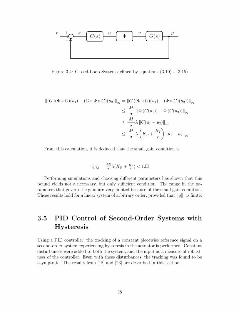
Figure 3.4: Closed-Loop System defined by equations (3.10) - (3.15)
‖(G Φ C)(u1)− (G Φ C)(u2)‖∞ = ‖G ((Φ C)(u1)− (Φ C)(u2))‖∞
≤ |M |σ‖Φ (C(u1))− Φ (C(u2))‖∞
≤ |M |σλ ‖C(u1 − u2)‖∞
≤ |M |σλ
(KP +
KI
ε
)‖u1 − u2‖∞ .
From this calculation, it is deduced that the small gain condition is
γ1γ2 = |M |σλ(KP + KI
ε) < 1.
Performing simulations and choosing different parameters has shown that thisbound yields not a necessary, but only sufficient condition. The range in the pa-rameters that govern the gain are very limited because of the small gain condition.These results hold for a linear system of arbitrary order, provided that ‖g‖1 is finite.
3.5 PID Control of Second-Order Systems with
Hysteresis
Using a PID controller, the tracking of a constant piecewise reference signal on asecond-order system experiencing hysteresis in the actuator is performed. Constantdisturbances were added to both the system, and the input as a measure of robust-ness of the controller. Even with these disturbances, the tracking was found to beasymptotic. The results from [18] and [23] are described in this section.
38

Figure 3.5: Closed-Loop System defined by equations (3.21) and (3.22)
3.5.1 Model
The spring-mass-damper system is a classical example of a physical system modeledby differential equations. The standard model without the presence of disturbancesor controlling forces is described by
mx′′(t) + cx′(t) + kx(t) = 0, x(0) = x0, v(0) = v0 (3.20)
where
m is the mass of the object,c is the damping constant,k is the linear spring constant, andx(t) is the displacement at time t.
The parameters m, c, and k must all be positive. The control to be used is aPID controller. Letting e(t) = x(t)− r,
u(t) = −KP e(t)−KI
∫ t
0
e(τ)dτ −KDd
dt(e(t)) + u0, u(0) = u0. (3.21)
As discussed previously, the input to the system will exhibit hysteresis. Two con-stant disturbances d1, d2 are introduced as a measure of robustness to the controller.See Figure 3.5, G(s) is the second-order system described in equation 3.20. Themodified system will have the form:
mx′′(t) + cx′(t) + kx(t) = Φ(u(t) + d2) + d1, x(0) = x0, (3.22)
x′(0) = v0, and u(0) = u0
3.5.2 Assumptions on Hysteresis Operators
Some further assumptions are required in order to achieve the results found in thetheorems in the next sections. There are six in total, but some necessary notation
39

must first be introduced.
Definition 3.5.1. Let W 1,1loc (R+) denote the space of locally absolutely continuous
functions. A function f ∈ W 1,1loc (R+) if there exists g ∈ L1
loc(R+) such that
f(t) = f(0) +
∫ t
0
g(s)ds for all t ∈ R+.
This is a smaller space than the set of continuous functions. According to thedefinition above, functions in this set must be locally L1-differentiable. That is,on any interval, the derivative must be defined and bounded almost everywhere.Throughout this section, θ will denote the step function, that is θ(t) = 1, for allt ≥ 0.
For w ∈ C([0, α]), α ≥ 0, γ, δ > 0,
B(w; δ, γ) := v ∈ C([0, α + γ]) : v|[0,α] = w, maxt∈[α,α+γ]
|v(t)− w(α)| ≤ δ. (3.23)
With these notational definitions in place, the following assumptions can bestated.
For a hysteresis operator Φ : C(R+)→ C(R+),
(N1) If u ∈ W 1,1loc (R+), then Φ(u) ∈ W 1,1
loc (R+)
The hysteresis operator must map continuous functions that have boundedderivatives almost everywhere to the same space of functions.
(N2) For u ∈ W 1,1loc (R+), Φ satisfies:
(Φ(u))′(t)u′(t) ≥ 0, a.e. t ∈ I,
where a.e. means almost everywhere, and I is the domain of definition of u. SinceΦ(u) depends on u, the following is implied:
u′(t) > 0 implies (Φ(u))′(t) ≥ 0, andu′(t) < 0 implies (Φ(u))′(t) ≤ 0
40
wherever u′(t) is defined.
(N3) Φ is locally Lipschitz in the following manner: there exists λ > 0 suchthat for all α ≥ 0 and w ∈ C([0, α]), there exists constants γ, δ > 0 such that
maxt∈[α,α+γ]
|(Φ(u))(t)−(Φ(v))(t)| ≤ λ maxt∈[α,α+γ]
|u(t)−v(t)|, for all u, v ∈ B(w; δ, γ).
Many hysteresis operators will satisfy a stronger condition, that is, a globalLipschitz condition
supt∈R+
|(Φ(u))(t)− (Φ(v))(t)| ≤ λ supt∈R+
|u(t)− v(t)|, for all u, v : C(R+) −→ R+.
holds. If this is true, then (N3) is obviously true.
(N4) For all α ∈ R+ and all u ∈ C([0, α]), there exists c > 0 such that
maxτ∈[0,t]
|(Φ(u))(τ)| ≤ c(1 + maxτ∈[0,t]
|u(τ)|), for all t ∈ [0, α).
The last two assumptions require some simple definitions.
Definition 3.5.2. The numerical value set, denoted NVS (Φ) represents all thepossible values that Φ can output.
Definition 3.5.3. A function f is ultimately non-decreasing (non-increasing)if there exists τ ∈ R+ such that f is non-decreasing (non-increasing) on [τ,∞).
Definition 3.5.4. A function f is approximately ultimately non-decreasing(non-increasing) if for all ε > 0, there exists τ > 0 and an ultimately non-decreasing(non-increasing function g such that for all t > τ ,
|f(t)− g(t)| < ε
The term approximately ultimately non-decreasing (non-increasing) is a broaderdefinition than ultimately non-decreasing (non-increasing) since functions that havedecaying oscillations (even if they continue to oscillate as t→∞) are included.
(N5) If u ∈ R+ is approximately ultimately non-decreasing and limt→∞
u(t) = ∞,
then (Φ(u))(t) and (Φ(−u))(t) converge to sup NVS Φ and inf NVS Φ, respectivelyas t→∞.
41
(N6) If, for u ∈ C(R+), limt→∞
(Φ(u))(t) is in the interior of NVS Φ, then u is bounded.
The assumption (N4) is a limiting growth condition on Φ, relative to u. As-sumptions (N5) and (N6) are similar in the sense that the behaviour of Φ mustin some sense follow the behaviour of u.
These assumptions will be referred to frequently throughout the remainder ofthe section and will be required in proofs involving specific systems. Commonlyused hysteresis operators that satisfy (N1) - (N6) include the backlash operator,elastic-plastic operator, and with some slight modifications (discussed later), thePreisach operator (see Section 3.5.3).
3.5.3 Comparison of Assumptions from Valadkhan/MorrisPaper and Logemann Papers
A comparison of the assumptions on the hysteresis operator found in [41] and [18]will be made. As in their respective sections, the assumptions found in [41] will bedenoted (A1)-(A4), while those found in [23] and [18] will be denoted (N1)-(N6).For consistency, u(t) will be the input to the hysteresis operator, and y(t) = Φ(u(t))will be the output. The first comparison deals with (A1) and (N1). They are asfollows:
(A1) If u(t) is continuous, then y(t) is continuous.
(N1) If u(t) ∈ W 1,1loc (R+), then y(t) ∈ W 1,1
loc (R+),
where W 1,1loc (R+) is the space of functions that are continuous and have a derivative
in L1(R+). At first glance, the two assumptions look very similar, however (N1)deals with a smaller space than (A1). It is important to note that neither assump-tion implies the other.
Next, a comparison is made between (A2) and (N3), which both deal with theLipschitz property of Φ acting on functions in B1(w, t1, t2) and B(w, δ, γ) respec-tively. The sets B1 and B are similar, with different names for the parameters.(A2) provides a global Lipschitz condition for Φ, while (N3) is only a local Lips-chitz condition (on Φ). Technically, (A2) is stronger. Following the introductionof (N1)-(N6), [18] also describes a global Lipschitz condition, that is identical to(A2).
(A3) will now be compared to (N2):
42

(A3) Consider an arbitrary interval [ti, tf ]. If for every t ∈ [ti, tf ], u(ti) ≥ u(t), theny(ti) ≥ y(tf ). Alternative, if for every t ∈ [ti, tf ], u(ti) ≤ u(t), then y(ti) ≤ y(tf ).
(N2) For u ∈ W 1,1loc (R+), Φ satisfies:
(Φ(u))′(t)u′(t) ≥ 0,
wherever u′(t) is defined. Recall that this is equivalent to whenever u(t) is increas-ing, Φ(u(t)) is nondecreasing, and whenever u(t) is decreasing, Φ(u(t)) is nonin-creasing. Since the interval in (A3) can be chosen arbitrarily, setting t = tf inthe assumption yields that monotonicity in the sense of (N2) is preserved. There-fore, (A3) implies (N2). The converse is not satisfied, since (A3) allows only forcounter-clockwise loops while clockwise loops are not permitted. Assumption (N2)does not imply (A3). Also note that in (A3), there are no assumptions regardingthe derivative of u(t) and Φ(u(t)) whereas these are required for (N2).
The remainder of this section will show that (A4) either implies, or is a specificcase of each of (N4)-(N6). Recall that (A4) deals with the saturation of thesystem:
(A4) There exists some usat > 0, y+, and y− such that if u(t) ≥ usat, thenΦ(u(t)) = y+, and Φ(−u(t)) = y−.
First, a comparison to (N4) will be made:
(N4) For all α ∈ R+, and all u ∈ C([0, α]), there exists c > 0 such that
maxτ∈[0,t]
|(Φ(u))(τ)| ≤ c(1 + maxτ∈[0,t]
|u(τ)|), for every t ∈ [0, α).
Assumption (N4) places a bound on growth of Φ(u(t)) that depends on u(t).It is immediately obvious that (N4) does not imply (A4), since an input u(t) canbe chosen that increases to infinity, resulting in y(t) not having a finite bound ony(t) as required by (A4). Recall that from Theorem 3.3.5, assumptions (A3) and(A4) together imply that there exist y+ and y− such that y− ≤ y(t) ≤ y+ for everyt ≥ 0. To show that this implies (N4),
Let c = max|y+|, |y−|.
43
maxτ∈[0,t]
|(Φ(u))(τ)| = maxτ∈[0,t]
|y(τ)|
≤ c,
≤ c+ c maxτ∈[0,t]
|u(τ)|,
= c(1 + maxτ∈[0,t]
|u(τ)|).
Therefore assumptions (A3) and (A4) imply assumption (N4).
In comparison to (N5), (A4) is a specific case of (N5).
(N5) If u ∈ R+ is approximately ultimately non-decreasing, and limt→∞
u(t) = ∞,
then Φ(u(t)) and Φ(−u(t)) will converge to sup NVS Φ, and inf NVS Φ respectively,as t→∞.
Assuming (A4) yields: if limt→∞
u(t) = ∞, then limt→∞
Φ(u(t)) = sup NVSΦ = y+,
and limt→∞
Φ(−u(t)) = inf NVSΦ = y−, hence satisfying (N5). (A4) guarantees that
sup NVS Φ and inf NVS Φ are reached by a finite u(t), whereas in (N5) sup NVSΦand inf NVSΦ need not be finite, and there need not exist a usat as described in(A4). Thus Assumption (A4) implies Assumption (N5). The converse is obvi-ously not true.
Finally, it will be shown that assumptions (A3) and (A4) together imply (N6):
(N6) If for u ∈ C(R+), limt→∞
Φ(u(t)) ∈ int NVS Φ, then u is bounded.
Assumptions (A3) and (A4) (see Theorem 3.3.5) imply that NVS Φ = [y−, y+].This property along with the contrapositive of (A4) yields that if y ∈ (y−, y+), then|u(t)| < usat. Hence, u is bounded. Therefore assumptions (A3) and (A4) implyassumption (N6). The converse is not true. It is clear that assumption (N6) doesnot imply (A3). To compare assumption (N6) with assumption (A4), if NVS Φis not a finite interval, then usat as described in assumption (A4) does not exist.If NVS Φ is a finite interval, then the contrapositive of (N6) only guarantees thatfor an unbounded u ∈ C(R+), sup NVS Φ or inf NVS Φ is reached as u approachesinfinity. This does not assert the existence of a usat. This is weaker than (A4)which guarantees that y+ or y− are reached as soon as |u(t)| ≥ usat.
Also note that assumptions (N1) - (N6) can have NVS Φ = (−∞,∞), whereasassumptions (A1) - (A4) cannot.
44
To summarize the comparisons:
(A1) acts on a larger space than (N1) but the assumptions do not imply each other.
(A2) implies (N3), (if the signals u and y are differentiable),
(A3) implies (N2),
(A3) and (A4) imply (N4)− (N6).
3.5.4 Integral Control In The Presence Of Hysteresis InThe Input
A simplified version of a result found in [23, Thm 4.1] is presented. (In referenceto the original paper, h, ϑ, ψ, g and u in [23] are replaced with 0, 0, the identitymap, η, and x respectively.) The introduction of a space of functions similar tothe Lp-space is required. Let Lpα(R+) denote the space of α-exponentially weightedfunctions. That is, f ∈ Lpα(R+) if∫ ∞
0
(f(t)e−αt)pdt <∞.
Also,
‖f‖Lpα(R+) =∥∥f(·)e−α·
∥∥p.
This is the space of functions that decrease faster than an exponential functionwith constant α < 0.
Let G : L2(R+)→ L2(R+) be a linear, bounded, shift-invariant operator definedby Gu = g ? u, where g ∈ L1
α(R+) + Rδ0 for some α < 0. The transfer function of Gis the Laplace transform of g, (denoted g). Note that g ∈ H∞(C+). The followingassumptions are made on g.
Assumption 3.5.5. [23, Assumption (L)] Let g satisfy
g(0) := lims→0,Re s>0
g(s) exists , g(0) > 0, and,
lim sups→0,Re s>0
∣∣∣∣ g(s)− g(0)
s
∣∣∣∣ <∞.The material presented in this section is entirely done by Logemann and his
associates. His work can be broken down into successive theorems, which are eachsteps to the final product.
45

Proposition 3.5.6. [23, Prop 2.1] Assume there are G, N , and r such that
(a) G : L2(R+)→ L2(R+) satisfies assumption 3.5.5;(b) N : R+ × R→ R satisfying
0 ≤ N(t, ξ)ξ ≤ aξ2, for every (t, ξ) ∈ [t0,∞)× R
(c) r ∈ L2(R+) + Rθ.
If v is a global solution to
v(t) = r(t)−∫ t
0
(G(N(·, v)))(τ)dτ
then
(i) v − r ∈ L∞(R+);
(ii) N(·, v) ∈ L2(R+);
(iii)
∫ t
0
N(τ, v(τ))dτ converges to a finite limit as t→∞.
Before proving results regarding the system presented in the next theorem, itis necessary to establish the existence and uniqueness of a solution for the system.Since the proof is rather long, it will be presented in Appendices A.1 and A.2. Theactual existence and uniqueness proof is for a more general system (Appendix A.1).It is shown in Appendix A.2 that the system (3.25) is a special case of the systemin Appendix A.1. The proof uses a standard ODEs argument that asserts theexistence and uniqueness of a solution on a small interval by using the contractionmapping theorem. Further arguments are made to extend uniqueness to all of R+.
The following lemmas will be referred to in the proof of the next theorem. Forthe first lemma, it can intuitively thought that f2 ultimately dominates f3.
Lemma 3.5.7. [23, Lemma 2.2] Let g ∈ W 1,1loc (R+) satisfy
g′ = f1(f2 − f3), (3.24)
where f1 /∈ L1(R+) is non-negative and bounded, limt→∞
f2(t) = l 6= 0 and f3 ∈Lp(R+), where 1 ≤ p <∞. Then the following statements hold.
1. If l < 0, then g is approximately ultimately non-increasing and limt→∞
g(t) =
−∞.
2. If l > 0, then g is approximately ultimately non-decreasing and limt→∞
g(t) =∞.
46
Lemma 3.5.8. [21, Lemma 3.2c)] Let Φ : C(R+) → C(R+) be a hysteresis oper-ator satisfying (N1) - (N6), with Lipschitz constant λ. For any u ∈ W 1,1
loc (R+),there exists a measurable function du : R+ → [0, λ] such that
(Φ(u))′(t) = du(t)u′(t), a.e. t ∈ R+.
Theorem 3.5.9. [23, Thm 4.1] Consider the system
x′ = κ(ρ− η − (G Φ)(x)), x(0) = x0 (3.25)
with the following assumptions:
1. G : L2(R+) → L2(R+) is a linear, bounded, and shift-invariant operator, asdescribed above, satisfying Assumption 3.5.5;
2. η ∈ L2(R+);
3. Φ is a hysteresis operator, satisfying (N1) - (N6) with associated Lipschitzconstant λ1;
4. There exists µ ∈ NVS Φ such that ρ = g(0)µ;
5. κ : R+ → R is measurable, non-negative and bounded with:
lim supt→∞
κ(t) <1
λ1|f(g)|,
where f(g) = infω∈R∗
Re
(g(iω)
iω
).
Then there exists a unique solution x ∈ W 1,1loc (R+) to (3.25) and the following
statements hold:
1. (Φ(x))′ ∈ L2(R+) and the limit Φ∞ := limt→∞
(Φ(x))(t) exists and is finite.
2. The signal w = η+ (G Φ)(x) can be decomposed into w = w1 +w2 where w1
is continuous and has a finite limit:
w∞1 = limt→∞
w1(t) = g(0)Φ∞,
and w2 ∈ L2(R+). Under the additional assumption that:
limt→∞
(η(t) + Φ(x(0))(Gθ(t)− g(0))) = 0, (3.26)
47
limt→∞
w2(t) = 0.
3. If κ /∈ L1(R+), then w∞1 = ρ and the error signal e = ρ−w can be decomposedas e = e1 +e2 where e1 is continuous and e2 ∈ L2(R+). If additionally, (3.26)holds, then lim
t→∞e(t) = 0.
4. If µ described in the assumptions is in the interior of NVS Φ, then x isbounded.
Proof.[Proof of Theorem 3.5.9] Each result in the theorem will be shown sepa-rately.
(1) The aim here is to apply Proposition 3.5.6 to the signal
w := w − ρ = η + (G Φ)(x)− ρ.
By the assumptions in the theorem, there exists µ such that ρ = g(0)µ. By Lemma3.5.8,
(Φ(x))′(t) = dx(t)x′(t)
= dx(t)κ(t)(ρ− η − (G Φ)(x))
= −dx(t)κ(t)w(t).
Define N(t, ξ) = κ(t)dx(t)ξ. Integrating yields
(Φ(x))(t) = (Φ(x))(0)−∫ t
0
N(τ, w(τ))dτ .
Applying the operator G on both sides yields
(G Φ(x))(t) = G(Φ(x(0))θ)(t)− G(∫ t
0
N(τ, w(τ))(τ)dτ
).
By linearity and shift-invariance of G,
(G Φ(x))(t) = (Φ(x(0)))(Gθ)(t)−∫ t
0
(G(N(τ, w(τ))))(τ)dτ
Adding η − g(0)µ to both sides,
(G Φ(x))(t) + η(t)− g(0)µ = η − g(0)µ+ Φ(x(0))(Gθ)(t)−∫ t
0
G(N(·, w))(τ)dτ.
(3.27)Defining
48

r := η − g(0)µθ + (Φ(x))(0)Gθ,
equation (3.27) can be written
w(t) = r(t)−∫ t
0
G(N(τ, w(τ)))(τ)dτ. (3.28)
Equation (3.28) has the same form as that found in Proposition 3.5.6. It remains toverify that the hypotheses on the components of (3.27) hold. Consider an operatorH: L2
loc(R+)→ L2loc(R+) defined by:
(Hv)(t) :=
∫ t
0
(Gv(τ)− g(0)v(τ))dτ. (3.29)
where G is the previously described convolution operator. The transfer functionof H is the Laplace transform of the corresponding function h. This is given by
h(s) =g(s)− g(0)
s. Note also that the inverse Laplace transform of h is the function
Gθ − g(0)θ. It is clear from Assumption 3.5.5 that h ∈ H∞(C+). It can also beshown that h ∈ H2(C+). Let r > 0. For Re(s) > 0 and |s| > r,
|h(s)| =∣∣∣∣ g(s)− g(0)
s
∣∣∣∣≤
supRe(s)>0
|g(s)|+ supRe(s)>0
|g(s)|
|s|
=2||g||H∞|s|
=
(1 + |s||s|
)2||g||H∞1 + |s|
=
(1
|s|+ 1
)2||g||H∞1 + |s|
≤(
1
r+ 1
)2||g||H∞1 + |s|
=M1
1 + |s|
where M1 = 2(1r
+ 1)||g||H∞ . For |s| < r and Re(s) > 0,
|h(s)| ≤ ||h||H∞
=(1 + |s|)||h||H∞
1 + |s|
≤ (1 + r)||h||H∞1 + |s|
=M2
1 + |s|.
49
where M2 = (1 + r)||h||H∞ . Choose γ = maxM1,M2. By Assumption 3.5.5and g, h ∈ H∞(C+), γ <∞. The transfer function h is bounded by γ
1+|s| for all of
Re(s) > 0. It is clear that this transfer function belongs in H2(C+), so h ∈ H2(C+).
By the Paley-Wiener Theorem [8, Appendix 6.21], Gθ− g(0)θ ∈ L2(R+), whichconsequently implies that Gθ ∈ L2(R+) + Rθ since g(0) ∈ R. Thus the first andthird conditions in Proposition 3.5.6 are satisfied. To show the second condition,note that
0 ≤ N(t, ξ)ξ ≤ λ1κ(t)ξ2.
By the assumption on κ (assumption 5 in the theorem statement), there exists0 < a < 1/|f(G)| and t0 ≥ 0 such that
0 ≤ N(t, ξ)ξ ≤ aξ2, for every (t, ξ) ∈ [t0,∞)× R.
Thus Proposition 3.5.6 can be applied, yielding that N(·, w) ∈ L2(R+) and thelimit of
∫ t0N(τ, w(τ))dτ as t→∞ exists and is finite. Hence (Φ(x))′ = −N(·, w) ∈
L2(R+), and
limt→∞
(Φ(x))(t) = (Φ(x))(0)− limt→∞
∫ t
0
N(τ, w(τ))dτ
exists and is finite, which proves the first result of Theorem 3.5.9.
(2) Let w1 := g(0)Φ(x) and let w2 := η + (Φ(x))(0)(Gθ − g(0) +H((Φ(x))′). Notethat
(H(Φ(x))′)(t)
=
∫ t
0
(G (Φ(x))′(τ)− g(0)(Φ(x))′(τ)) dτ
= (G Φ)(x(t))− (G Φ)(x(0))− g(0) [(Φ(x))(t)− (Φ(x))(0)] .
It is easily verified that w1 and w2 form a valid decomposition of w. By re-sult (1), w∞1 := g(0)Φ∞ exists and is finite. Considering the components of w2,η ∈ L2(R+), and from the proof of result (1), it was argued by the Paley-WienerTheorem (see [8, Appendix 6.26]) that Gθ− g(0)θ ∈ L2(R+). Also, by Assumption3.5.5, h ∈ H∞(C+), which implies that H maps L2(R+) to itself. From result (1),(Φ(x))′ ∈ L2(R+), so H(Φ(x))′) ∈ L2(R+). Therefore w2 ∈ L2(R+).
With the additional assumption described in the result of (2), the first twoterms of w2 → 0 as t → ∞. It remains to show that lim
t→∞(H(Φ(x)′))(t) = 0.
Since H is bounded, linear, and shift-invariant, there exists a function h where
50

H((Φ(x))′) = h ? (Φ(x))′. Again by the Paley-Wiener Theorem (see [8, Appendix6.26]), h (whose Laplace transform is in H2(C+)) belongs in L2(R+). From Ap-pendix C of [9], the term (H(Φ(x)′))(t) is a convolution of two functions in L2(R+)and hence has a zero limit.
(3) Rewrite the system (3.25) as
x′ = κ(ρ− w1 − w2). (3.30)
The aim is to prove limt→∞
w1 = w∞1 = ρ. Suppose w∞1 > ρ. Lemma 3.5.7 can be used
with g = x, f1 = κ, f2 = ρ− w1 and f3 = w2. Then x is approximately ultimatelynon-increasing and lim
t→∞x(t) = −∞. Hence by (N5),
limt→∞
Φ(x(t)) = Φ∞ = inf NVS Φ.
Since it was assumed in the theorem statement that µ ∈ NVS Φ,
ρ = g(0)µ ≥ g(0)Φ∞ = w∞1 .
A contradiction is reached. If the same argument is made for w∞1 < ρ, the conclu-sion that w∞1 = ρ is reached. Finally, in letting e1 = ρ − w1 and e2 = −w2, therequired decomposition for the additional property that lim
t→∞e(t) = 0 is achieved.
(4) Two cases will be considered independently based on whether or not κ belongsto L1(R+). Suppose it does, considering the system in the form above in (3.30), w1
is bounded, and w2 ∈ L2(R+). By the fact that κ ∈ L1(R+) and that it is bounded,the L2-norm of κ must also be bounded. Note that
‖κ‖2 =
(∫ ∞0
(κ(t))2dτ
) 12
≤(
maxt∈[0,∞)
|κ(t)|)1/2(∫ ∞
0
|κ(t)|dτ)1/2
= ‖κ‖12∞ ‖κ‖
121
<∞
Finally, κ(ρ − w1 − w2) will be shown to belong to L1(R+). For the first twoterms, ρ and w1 are both bounded so κρ and κw1 both belong to L1(R+). For thelast term, an appeal is made to Holder’s inequality. Since both κ and w2 are inL2(R+),
‖κw2‖1 ≤ ‖κ‖2 ‖w2‖2 <∞.
51
Hence x′ ∈ L1(R+), and is integrable and hence x is bounded. If κ /∈ L1(R+),then by result (3), w1(t) → ρ as t → ∞. Therefore w1 = g(0)Φ(x) implies thatΦ∞ ∈ int(NVS(Φ)). By (N6), x is bounded.
Next, the main result of the section is presented.
Theorem 3.5.10. [18, Thm 3.2] Let g ∈ L1α(R+) + Rδ0 for some α < 0, where δ0
is the Dirac distribution with support at 0. Let r1, r2 ∈ R, κ > 0 and q ∈ L2(R+)with lim
t→∞q(t) = 0.
Let Φ : C(R+) → C(R+) be a hysteresis operator that satisfies assumptions(N1) - (N6) with associated Lipschitz constant λ > 0.
Let g denote the Laplace Transform of g, and g(0) > 0, r1 +r2
g(0)∈ NVS Φ,
and define f(g) = infω∈R∗
Re
(g(iω)
iω
). For every κ such that
0 < κ <
1
λ|f(g)| , f(g) 6= 0
∞, f(g) = 0, (3.31)
and y0 ∈ R, there exists a unique solution y ∈ W 1,1loc (R+) to
y′ = κ(r1(g ? θ) + q + r2θ − (g ? Φ(y))), y(0) = y0 ∈ R, (3.32)
such that limt→∞
y′(t) = 0, and limt→∞
(Φ(y))(t) = r1 +r2
g(0)and (Φ(y))′ ∈ L2(R+).
Moreover, if r1 +r2
g(0)∈ int NVS Φ, then y is bounded.
This result is pertinent because it describes asymptotic properties and will beuseful in showing asymptotic tracking in the next theorem. Theorem 3.5.10 statesthe limit of the hysteresis operator and guarantees that the solution of the differ-ential equation (3.32) tends to zero as t tends to infinity.
Proof: It will be shown that this current setup satisfies the previous theoremwith (3.32) taking the role of (3.25). First, since g ∈ L1
α(R+) + Rδ0 with α < 0,hence g is holomorphic and bounded on the open right-half plane. Furthermore,−tg(t) ∈ L1
α(R+) + Rδ0 since the exponential decay will eventually dominate thepolynomial factor. Its Laplace transform g′(s) must also exist, and
|g′(0)| <∞, and
lim sups→0,Re s>0
∣∣∣∣ g(s)− g(0)
s
∣∣∣∣ = |g′(0)|
52
From the assumptions of this theorem g(0) > 0 thus Assumption 3.5.5 is satis-fied. Next, by the Final Value Theorem, g ? θ − g(0)→ 0 as t→∞ where θ is theunit step function. Also g ? θ− g(0) ∈ L2(R+) by the Paley-Wiener Theorem, sinceits Laplace transform is in H2(C+). Comparing (3.32) with the system found inTheorem 3.5.9, let ρ = g(0)r1 + r2 and η = r1(g(0)− g ? θ)− q, which is in L2(R+)since each term is in L2(R+).
Therefore Theorem 3.5.9 can be applied to (3.32). The properties limt→∞
y′(t) = 0,
(Φ(y))′ ∈ L2(R+), and limt→∞
(Φ(y))(t) exists are true. Moreover, y is bounded,
provided that r1 + r2g(0)
is an interior point of NVS Φ. Finally, it is claimed that
Φ∞ = r1 + r2/g(0). This can be verified from equation (3.32) by applying theproperties shown already. As t → ∞, y′(t) → 0, q → 0, (g ? θ)(t) → g(0) and(g ? Φ(y))(t) → g(0)Φ∞ by use of the Final Value Theorem. As t → ∞, equation(3.32) becomes
0 = κ(r1g(0) + r2 − g(0)Φ∞)
Dividing both sides by κ and rearranging the terms yields
Φ∞ = r1 +r2
g(0).
3.5.5 PID Control of Systems with Hysteresis
In this section, asymptotic tracking of the system (3.22) is presented. See Figure3.5. The transfer function G(s) is the second-order system described in equation(3.22). It is shown that through the manipulation of the control parameters, the de-sired closed-loop properties can be achieved even without the presence of derivativecontrol.
Theorem 3.5.11. [18, Thm 4.3] Let Φ : C(R+)→ C(R+) be a hysteresis operatorsatisfying (N1) - (N6), with associated Lipschitz constant λ > 0. Let r, d1, d2 ∈ Rand assume that rk − d1 ∈ NVS Φ. Consider two cases,
Case (a): KD = 0 and KP , KI > 0 such that
(A) 0 < KI <KP kc
< ckλm.
Case (b): KP , KI , KD > 0 such that
(B1) 0 < KI <∞,
(B2) KP >cKI
k,
53

(B3) KD >mKP
c,
Then there exists a unique solution x ∈ C2(R+) of the closed-loop system givenby (3.22) such that
limt→∞
x(t) = r , limt→∞
x′(t) = 0, limt→∞
x′′(t) = 0, limt→∞
(Φ(u+ d2θ))(t) = rk − d1
Moreover, if rk − d1 is an interior point of NVS Φ, then the control signal ugiven by (3.1) is bounded.
It is useful to know the steady-state result of the control under the hystereticeffects. Note that asymptotic tracking of a constant reference signal is the result ofthis theorem.
Proof. The aim of this proof is to demonstrate that the system satisfies the as-sumptions of Theorem 3.5.10. Several functions must first be defined and it will beshown that those functions live in the desired spaces.
Let p(s) := ms2 + cs+ k, let h be the solution of the initial value problem
p
(d
dt
)h = 0, h(0) = 0, h′(0) =
1
m,
and let ρ be the solution of the initial-value problem
p
(d
dt
)ρ = 0, ρ(0) = x0, ρ′(0) = v0.
By direct substitution, the function x
x = h ?[Φ(−KP (x− rθ)−KDx
′ −KI
∫ ·0(x(τ)− r)dτ + (u0 + d2)θ
)+ d1θ
]+ ρ,
satisfies the system (3.22). Define w(t) = u(t) + d2. The following calculation caneasily be verified by direct substitution. The Dirac distribution δ0 is the identityelement of convolution, and differentiation of a convolution yields: (g ? h)′(t) =g(t)h(0) + g ?h′ = g(t) ?h(0)δ0 + (g ?h′)(t) (see Appendix A.3). Thus, for all t ≥ 0,
w(t) = u(t) + d2
= −KP (x− r)−KDx′ −KI
∫ ·0
(x(τ)− r)dτ + u0 + d2.
Differentiating and defining
54
g :=KD
KI
[h′′ +
1
mδ0
]+KP
KI
h′ + h,
and
q := −KD
KI
ρ′′ − KP
KI
ρ′ − ρ.
yields
w′ = −KPx′ −KDx
′′ −KI(x− rθ) (3.33)
= KI(rθ + q − d1g ? θ − g ? Φ(w)), (3.34)
where
w(0) = −KP (x0 − r)−KDv0 + u0 + d2.
Note that w′ has the form of y′ in Theorem 3.5.10 with κ = KI , r1 = −d1, andr2 = r. With this setup in mind, the rest of the assumptions will be shown to hold.The denominator of both of the transfer functions of h and ρ is p(s), whose roots
are: −c±√c2−4km2
, which clearly have negative real part. The poles of the transferfunctions of h and ρ all lie in the left-half complex plane, which implies that thefunctions and their derivatives decay exponentially and are hence in L2(R+). SeeAppendix A.4 for a detailed explanation.
Because linear combinations of h, ρ and their derivatives are exponentially de-caying, q ∈ L2(R+) and lim
t→∞q(t) = 0, and g ∈ L1
α(R+) + Rδ0 for some α < 0. The
Laplace transform of g is
g(s) =1
KI
KDs2 +KP s+KI
ms2 + cs+ k.
Therefore g(0) = 1/k > 0. Also, by assumption rk − d1 = r2/g(0) + r1 ∈ NVS Φ.It remains to show that KI satisfies the role of κ as described in Theorem 3.5.10,by verifying (3.31). Consider
55
f(g) = infω∈R∗
Re
(g(iω)
iω
)= inf
ω∈R∗Re
(KD(iω)2 +KP iω +KI
KI(m(iω)3 + c(iω)2 + kiω)
)= inf
ω∈R∗Re
(−KDω
2 +KI +KP iω
KI(−cω2 + i(kω −mω3))· −cω
2 − i(kω −mω3)
−cω2 − i(kω −mω3)
)= inf
ω∈R∗1
KI
(KDcω
4 −KIcω2 +KPkω
2 −KPmω4
c2ω4 + (kω −mω3)2
), let ξ = ω2 vary from (0,∞)
= infξ∈R+
1
KI
((KPk −KIc) + ξ(KDc−mKP )
m2ξ2 + (c2 − 2mk)ξ + k2
)= inf
ξ∈R+
((KPk −KIc) + ξ(KDc−mKP )
KI((mξ − k)2 + c2ξ)
).
where ξ = ω2 and let ζ : R+ → R be defined by
ζ(ξ) =(kKP − cKI) + ξ(cKD −mKP )
KI((mξ − k)2 + c2ξ).
At this point, each of the two cases are considered separately and are each shownto satisfy (3.31).
Case (a): Let KD = 0, and assume (A) holds. From (A), kKP − cKI > 0. Thedenominator of ζ is positive for all ξ ≥ 0. Since KD = 0, if ξ > kKP−cKI
mKP, then
ζ(ξ) < 0. Thus f(g) defined above is negative. Also,
f(g) ≥ infξ∈R+
µ(ξ),
where µ(ξ) :=−mKP ξ
KI((mξ − k)2 + c2ξ). The function µ attains a global minimum over
R+ at ξ = k/m, and hence
0 > f(g) ≥ µ(k/m) = −mKP
c2KI
.
By (A), 1 < c2/(λmKP ), hence
56
0 < KI <KIc
2
λmKP
≤ 1
λ|f(g)|.
Thus, if KD = 0, (3.31) is satisfied by choosing κ = KI .
It remains to show that the hypothesis holds for Case b). Let KP , KI , KD > 0and (B1), (B2), (B3) hold, then both terms in the numerator of ζ are positive,as is the denominator, so ζ(ξ) ≥ 0 for all ξ ∈ R+. Along with f(g) = lim
ξ→∞ζ(ξ) = 0,
KI = κ can take on any real value, hence the assumption in equation (3.31) issatisfied.
Therefore, all the hypotheses of Theorem 3.5.10 are satisfied. Hence, there ex-ists a unique solution w ∈ C1(R+) to (3.34), such that w′(t)→ 0 and (Φ(w))(t)→rk − d1 as t→∞. Finally, consider (3.34),
KDe′′ +KP e
′ +KIe = −w′,
with −w′ as the input to the system. Since KP , KI > 0, and KD ≥ 0 and w′(t)→ 0as t → ∞ (shown above), e(t) → 0 (that is, x(t) → r). By an application of theFinal Value Theorem, e′(t) = x′(t) → 0 as t → ∞. From equation (3.33), ast approaches ∞, x′′(t) approaches 0 since all the other components decay to 0.Finally, if r1 + r2/g(0) = −d1 + rk ∈ int NVS Φ, then boundedness of w, and henceby its definition, boundedness of u follows.
3.6 Verification of Results for First-Order Sys-
tem
The work presented in [18] is in the context of second-order systems. A verifica-tion that the results hold true for a first-order system is given here. Logemann’sapproach (building on successive theorems) will be especially useful in this context.As in the previous setup, u(t) is the PID controller (3.21). Consider
Mx′(t) + σx(t) = Φ(u(t) + d2) + d1, x(0) = x0. (3.35)
The results of applying Theorem 3.5.10 to the first-order system (3.35) are sum-marized in the following corollary.
Corollary 3.6.1. Let Φ : C(R+)→ C(R+) be a hysteresis operator satisfying (N1)- (N6), with associated Lipschitz constant λ > 0. Let r, d1, d2 ∈ R and assume thatrσ − d1 ∈ NVS Φ. Let M , σ > 0. Consider two cases,
57
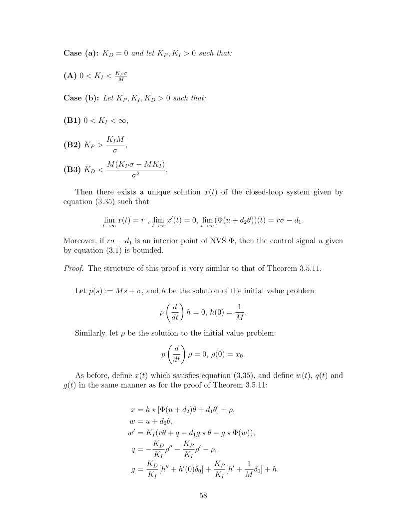
Case (a): KD = 0 and let KP , KI > 0 such that:
(A) 0 < KI <KP σM
Case (b): Let KP , KI , KD > 0 such that:
(B1) 0 < KI <∞,
(B2) KP >KIM
σ,
(B3) KD <M(KPσ −MKI)
σ2,
Then there exists a unique solution x(t) of the closed-loop system given byequation (3.35) such that
limt→∞
x(t) = r , limt→∞
x′(t) = 0, limt→∞
(Φ(u+ d2θ))(t) = rσ − d1.
Moreover, if rσ − d1 is an interior point of NVS Φ, then the control signal u givenby equation (3.1) is bounded.
Proof. The structure of this proof is very similar to that of Theorem 3.5.11.
Let p(s) := Ms+ σ, and h be the solution of the initial value problem
p
(d
dt
)h = 0, h(0) =
1
M.
Similarly, let ρ be the solution to the initial value problem:
p
(d
dt
)ρ = 0, ρ(0) = x0.
As before, define x(t) which satisfies equation (3.35), and define w(t), q(t) andg(t) in the same manner as for the proof of Theorem 3.5.11:
x = h ? [Φ(u+ d2)θ + d1θ] + ρ,
w = u+ d2θ,
w′ = KI(rθ + q − d1g ? θ − g ? Φ(w)),
q = −KD
KI
ρ′′ − KP
KI
ρ′ − ρ,
g =KD
KI
[h′′ + h′(0)δ0] +KP
KI
[h′ +1
Mδ0] + h.
58

Since ρ and h are exponentially decaying functions, q ∈ L2(R+) and g ∈L1α(R+) + Rδ0, for some α < 0. The Laplace transform of g yields
g(s) =1
KI
MKP s+MKI −KDsσ
M(Ms+ σ), where g(0) =
1
σ> 0.
It remains to show that κ, or in the present context KI , satisfies the requiredassumption in each of the cases, but first, a calculation of f(g) must be performed.Again, let
f(g) = infω∈R∗
Re
(g(iω)
iω
),
= infξ∈R+
(ζ(ξ)) .
Note that ξ = ω2 > 0. After some algebraic computations, the following be-comes the equation to be minimized:
ζ(ξ) =1
KI
−M2KI +MKPσ −KDσ2
M3ξ +Mσ2.
Case (a): Let KD = 0, and (A) hold. The third term in the numerator disap-pears. By condition (A), KP and KI must be chosen such that −MKI +KPσ > 0.Hence, the function ζ is always positive, and approaches 0 as ξ becomes arbitrarilylarge. The assumption (3.31) is satisfied with f(g) = 0.
Case (b): Let KD > 0, such that (B1), (B2) and (B3) hold. Under a similarargument as case (a), ζ is positive and ζ → 0 as ξ →∞.
Hence all the required assumptions are satisfied, and Theorem 3.5.10 can beapplied. By the same arguments used at the end of Theorem 3.5.11, the conclusionsof this corollary follow.
59

3.7 Other Forms of Control of Hysteretic Sys-
tems
While the work presented in this thesis is focused on the PID control of hystereticsystems, there has been some control work done outside of this area. A briefoverview of other methods of control applied to hysteretic systems will be presentedhere. The modeling of the hysteretic system may vary from paper to paper, andmay include models not mentioned in the modelling section. Several papers areconcerned with specific applications such as the control of magnetostrictives. Thefocus here is on the control method rather than the hysteresis model, and on theresults achieved (for example, stability and tracking).
3.7.1 Optimal Control
The optimal control problem is well known in the literature. Suppose there area set of differential equations that govern the dynamics of a system. The systemis subject to some inputs, and there are certain optimization criteria that needto be met. The optimal control law is the solution that satisfies the optimizationcriteria while at the same time minimizing a cost functional that is chosen basedon design parameters. For a physical example, consider the well-known invertedpendulum and cart system. There is a pendulum that is free to swing about anaxis of rotation, attached to a cart that can exhibit motion on a one dimensionaltrack. The control can accelerate the cart back and forth. Given an initial angle ofthe pendulum and starting reference point on the track, the optimization criteriarequires the system to balance the pendulum upright, while bringing the cart toa desired origin point. The state-space formulation considers four states: positionand velocity of each of the pendulum (angular quantities in this case) and the cart.The cost function is chosen to be some combination of those four quantities.
In [3], a general system is introduced that can contain hysteretic componentsmodeled by the Preisach model. They find viscosity solutions to the derivedHamilton-Jacobi-Bellman equation, which are solutions that can have points wherethe solution is not differentiable, but still satisfies the system in an appropriatesense. The value function is shown to be bounded. The same concept is evaluatedby the same author while considering the play operator and the Prandtl-Ishlinskiioperator in [2]. An example of a special case of optimal control, linear quadraticregulator, can be found in [31], applied to a hysteretic system.
3.7.2 Sliding Mode Control
Contrary to many other control theory formulations, the control law produced bysliding mode control is not continuous. The control switches between different
60
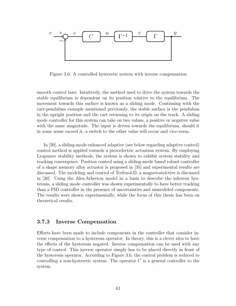
Figure 3.6: A controlled hysteretic system with inverse compensation
smooth control laws. Intuitively, the method used to drive the system towards thestable equilibrium is dependent on its position relative to the equilibrium. Themovement towards this surface is known as a sliding mode. Continuing with thecart-pendulum example mentioned previously, the stable surface is the pendulumin the upright position and the cart returning to its origin on the track. A slidingmode controller for this system can take on two values, a positive or negative valuewith the same magnitude. The input is driven towards the equilibrium, should itin some sense exceed it, a switch to the other value will occur and vice-versa.
In [20], a sliding-mode enhanced adaptive (see below regarding adaptive control)control method is applied towards a piezoelectric actuation system. By employingLyapunov stability methods, the system is shown to exhibit system stability andtracking convergence. Position control using a sliding-mode based robust controllerof a shape memory alloy actuator is proposed in [35] and experimental results arediscussed. The modeling and control of Terfenol-D, a magnetostrictive is discussedin [30]. Using the Jiles-Atherton model as a basis to describe the inherent hys-teresis, a sliding mode controller was shown experimentally to have better trackingthan a PID controller in the presence of uncertainties and unmodeled components.The results were shown experimentally, while the focus of this thesis has been ontheoretical results.
3.7.3 Inverse Compensation
Efforts have been made to include components in the controller that consider in-verse compensation to a hysteresis operator. In theory, this is a clever idea to havethe effects of the hysteresis negated. Inverse compensation can be used with anytype of control. This inverse operator simply has to be placed directly in front ofthe hysteresis operator. According to Figure 3.6, the control problem is reduced tocontrolling a non-hysteretic system. The operator C is a general controller to thesystem.
61
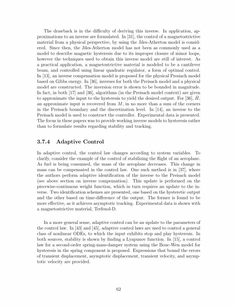
The drawback is in the difficulty of deriving this inverse. In application, ap-proximations to an inverse are formulated. In [31], the control of a magnetostrictivematerial from a physical perspective, by using the Jiles-Atherton model is consid-ered. Since then, the Jiles-Atherton model has not been as commonly used as amodel to describe magnetic hysteresis due to its improper closure of minor loops,however the techniques used to obtain this inverse model are still of interest. Asa practical application, a magnetostrictive material is modeled to be a cantileverbeam, and controlled using linear quadratic regulator, a form of optimal control.In [13], an inverse compensation model is proposed for the physical Presiach modelbased on Gibbs energy. In [36], inverses for both the Preisach model and a physicalmodel are constructed. The inversion error is shown to be bounded in magnitude.In fact, in both [17] and [36], algorithms (in the Preisach model context) are givento approximate the input to the hysteresis to yield the desired output. For [36], H,an approximate input is recovered from M , in no more than a sum of the cornersin the Preisach boundary and the discretization level. In [14], an inverse to thePreisach model is used to construct the controller. Experimental data is presented.The focus in these papers was to provide working inverse models to hysteresis ratherthan to formulate results regarding stability and tracking.
3.7.4 Adaptive Control
In adaptive control, the control law changes according to system variables. Toclarify, consider the example of the control of stabilizing the flight of an aeroplane.As fuel is being consumed, the mass of the aeroplane decreases. This change inmass can be compensated in the control law. One such method is in [37], wherethe authors perform adaptive identification of the inverse to the Preisach model(see above section on inverse compensation). This update is performed on thepiecewise-continuous weight function, which in turn requires an update to the in-verse. Two identification schemes are presented, one based on the hysteretic outputand the other based on time-difference of the output. The former is found to bemore effective, as it achieves asymptotic tracking. Experimental data is shown witha magnetostrictive material, Terfenol-D.
In a more general sense, adaptive control can be an update to the parameters ofthe control law. In [43] and [45], adaptive control laws are used to control a generalclass of nonlinear ODEs, to which the input exhibits stop and play hysteresis. Inboth sources, stability is shown by finding a Lyapunov function. In [15], a controllaw for a second-order spring-mass-damper system using the Bouc-Wen model forhysteresis in the spring component is proposed. Expressions that bound the errorsof transient displacement, asymptotic displacement, transient velocity, and asymp-totic velocity are provided.
62

Chapter 4
Simulations
Computations were performed using MATLAB R© to visualize and simulate some ofthe theory presented. Three hysteresis operators were considered: backlash, elastic-plastic and Preisach operators. As an application, one can consider the trackingof a certain signal (for example, constants, ramps, sinusoids etc.) by an actuatorthat exhibits hysteresis. Originally, Simulink R© was considered in performing thesesimulations however the programming of the Preisach model in Simulink provedto be a challenge. Instead, all of the simulations were performed in MATLAB R©
using a Runge-Kutta fourth order fixed-step ODE solver. The code is available inAppendix B.
4.1 System Description
Recall that the equations that govern the closed-loop system (3.10) - (3.15) are:
e(t) = r(t)− y(t),
u(t) = KP e(t) +KI exp(-εt)
∫ t
0
exp(ετ)e(τ)dτ,
v(t) = Φ(u(t)),
y′(t) = Mv(t)− σy(t),
where Φ represents the hysteresis operator. Refer to Figure 3.4, where G(s) = Ms+σ
.Since this is in fact a closed loop, the entire system can be rewritten as a singleequation, dependent on r(t) and y(t). This equation becomes
y′(t) = −σy(t) +MΦ
[KP (r(t)− y(t)) +KI exp(-εt)
∫ t
0
exp(ετ) (r(τ)− y(τ)) dτ
].
(4.1)
63

As mentioned above, the fourth-order Runge-Kutta numerical scheme is used.Note that equation (4.1) is written in the form y′(t) = f(t, y). Given yn, time tnand timestep h, the method to obtain yn+1 is the following,
k1 = f(tn, yn),
k2 = f(tn +1
2h, yn +
1
2hk1),
k3 = f(tn +1
2h, yn +
1
2hk2),
k4 = f(tn + h, yn + hk3),
k =1
6(k1 + 2k2 + 2k3 + k4)
yn+1 = yn + hk
tn+1 = tn + h.
A weighted average of the slopes k, considered at four different points varyingfrom tn to tn+1 is used to compute the next input value. Since the chosen methodwas an explicit scheme, a relatively small timestep was used. In all simulations thetimestep never exceeded h = 0.01s. The integral in Equation (4.1) is computed bya simple trapezoidal rule. This was chosen for the sake of computational simplicity.Finally, the history of the input u(t) in calculating k1 to k4 was chosen to not havean affect on another. To clarify, the input history used to calculate k1 to k4 is thesame. Only the last value of the input u(t) differed according to the definitions ofthe coefficients.
The numerical scheme was entirely self-written. Despite the superiority of thebuilt-in techniques available in MATLAB R©, an issue arose with the need to accessthe solution in previous timesteps as the solution was being computed. The outputfunction, y, was provided only at the end of the computation. Accessing previoustimesteps that the hysteresis operator required as the solution was being solvedproved to be a challenge. Regardless of whether or not this was possible throughmodifying the code, it was much quicker to implement a self-written solver.
4.2 Implementation of Hysteresis Operators
The implementation of the hysteresis operators is discussed in the following section.Both the backlash and the elastic operators are programmed to work very quickly,while the Preisach model being a much more complex and difficult model to im-plement, took longer to run, but less than thirty seconds to produce a ten-secondlong simulation on a dual 1.66 GHz Processor.
64

4.2.1 Backlash Operator and Elastic-Plastic Operator
Using the notation provided in its definition, recall that the backlash operatortakes the parameters ξ and h (denoted by bfac in the code) in addition to the inputhistory to determine its current value. The initial value is given by the parameterξ. The lagging factor h represents a dead zone, that the input must first overcomein order to see a change in the output. Upon close inspection, only the currentvalue of the input, as well as the two previous timesteps (rather than the entireinput history) are required. The need for the previous timesteps, is to determineif the input changes direction (from increasing to decreasing or vice versa). Shouldthe input change direction, the current interval would no longer be monotone. Anew interval must begin, that is, i = i + 1, ti = t, and Bh,ξ(u(ti)) is updated toBh,ξ(u(t)). The function bh is programmed exactly as it is defined.
The elastic-plastic operator is programmed in the same fashion. The code usesthe variable efac rather than h, since h is used for the timestep length. The onlydifference compared to the backlash operations was the need for the value of u(ti)in addition to Eh,ξ(u(ti)). Similar to the latter value, u(ti) is fed through the systemas an input and an output that changes only to u(t) should it change direction.The function eh was straightforward to program.
4.2.2 Preisach Operator
First, a gridsize and a saturation value usat of the input is chosen (recall assump-tion (A4)). Together, the two parameters determine the size of the array (2round( usat
gridsize), round( usat
gridsize) required to represent the Preisach plane. The top
right and bottom right portions are always 0, as they are not part of the Preisachplane. The grid is rotated compared to the original definition given in Section 2.3.This change facilitated the input of the Preisach plane into a matrix (see Figure 4.1).
At each time step, u(t) is provided. The cells affected by the boundary aremodified, and the corresponding cells that switch their relays are updated. Forexample, Figure 4.1 represents the an initialized Preisach plane with usat = 10 andgridsize = 1, where the input has been increased from u = 0 to u = 5. The planeand the boundary are both drawn onto the matrix. The model allows for cells totake values other than +1 and −1. Should the boundary traverse a cell, a fractionalvalue dependent on the amount of area in each of the +1 or the −1 regions is con-sidered. See Figure 4.2, the input has been monotonically increased from u = 0, tou = 7, then monotonically decreased to u = 2.5.
The weight function used is based on experimental data of Terfenol-D, a magne-tostrictive material. This data was obtained by Sina Valadkhan [39]. The methoddescribed previously where the Preisach plane is subdivided into square-shaped cellswhere a constant value is assumed over each cell is used. A detailed explanation of
65
Figure 4.1: MATLAB R© Preisach Plane at u = 5 (from u = 0)
Figure 4.2: MATLAB R© Preisach Plane: u = [0, 7, 2.5]
66

Figure 4.3: Preisach Major Loop with Terfenol-D Data
this weight function can be found in [39]. The weight function is a matrix of thesame size as the grid for the Preisach plane, which is then multiplied cell by cellwith the Preisach plane for a given input history. The sum of the entries of theresultant matrix is multiplied by the area of each grid. This value is the output ofthe Preisach model at that timestep. A major loop of the hysteresis can be foundin Figure 4.3. The reader is referred to Section 1.4 of [25] for an alternate numericalimplementation of the Preisach model.
4.3 Results
While the theory presented in this thesis does not cover the stability and trackingof ramps and sinusoids, their simulation is presented here to demonstrate the ef-fectiveness of a PI controller for these applications. The stability results found inSection 3.4 provide a range of parameters for which stability is guaranteed. Sincethe aim was to use a practical PI controller, the parameter ε was chosen to be smallto mimic a pure integral controller. It is shown however in Section 3.6 that for afirst order system, the conditions that had to be satisfied for asymptotic trackingwere
0 < KI <KPσ
Mand KP > 0.
67

Figure 4.4: Weight Function from Terfenol-D Data
The parameters σ = M = 1 were used in performing the simulations. Therequired conditions became 0 < KI < KP , KP > 0. The performance becamebetter for larger values of KI and KP provided that the necessary conditions weresatisfied. With practical application however, these parameters are limited by themaximum output of an actuator. It will be seen that these conditions are notnecessary, but only sufficient for stability.
4.3.1 Tracking a Constant Reference Signal
Backlash and Elastic-Plastic Operators
A reference signal of r(t) = 1 was tracked with the backlash and elastic-plasticoperators acting on the controller. In Figure 4.5, both the backlash factor and theelastic-plastic factor were set to 3 with 0 initial condition. The controller parameterswere chosen to be KP = 10, and KI = 5. In comparison to the controller actingwith no hysteresis, an overshoot is produced with the backlash operator. Thenature of the backlash operator is that the output is a delayed version of the input.When a larger control effort is required, the system must wait until the backlash isovercome. This delay in control effort causes the system to drift past the desiredvalue. The elastic-plastic operator has a limit in terms of control effort that can beexerted, resulting in the slower response seen in Figure 4.5.
Should the conditions be violated, the system may still be stable. The effect
68
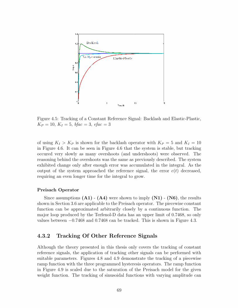
Figure 4.5: Tracking of a Constant Reference Signal: Backlash and Elastic-Plastic,KP = 10, KI = 5, bfac = 3, efac = 3
of using KI > KP is shown for the backlash operator with KP = 5 and KI = 10in Figure 4.6. It can be seen in Figure 4.6 that the system is stable, but trackingoccured very slowly as many overshoots (and undershoots) were observed. Thereasoning behind the overshoots was the same as previously described. The systemexhibited change only after enough error was accumulated in the integral. As theoutput of the system approached the reference signal, the error e(t) decreased,requiring an even longer time for the integral to grow.
Preisach Operator
Since assumptions (A1) - (A4) were shown to imply (N1) - (N6), the resultsshown in Section 3.6 are applicable to the Preisach operator. The piecewise constantfunction can be approximated arbitrarily closely by a continuous function. Themajor loop produced by the Terfenol-D data has an upper limit of 0.7468, so onlyvalues between −0.7468 and 0.7468 can be tracked. This is shown in Figure 4.3.
4.3.2 Tracking Of Other Reference Signals
Although the theory presented in this thesis only covers the tracking of constantreference signals, the application of tracking other signals can be performed withsuitable parameters. Figures 4.8 and 4.9 demonstrate the tracking of a piecewiseramp function with the three programmed hysteresis operators. The ramp functionin Figure 4.9 is scaled due to the saturation of the Preisach model for the givenweight function. The tracking of sinusoidal functions with varying amplitude can
69
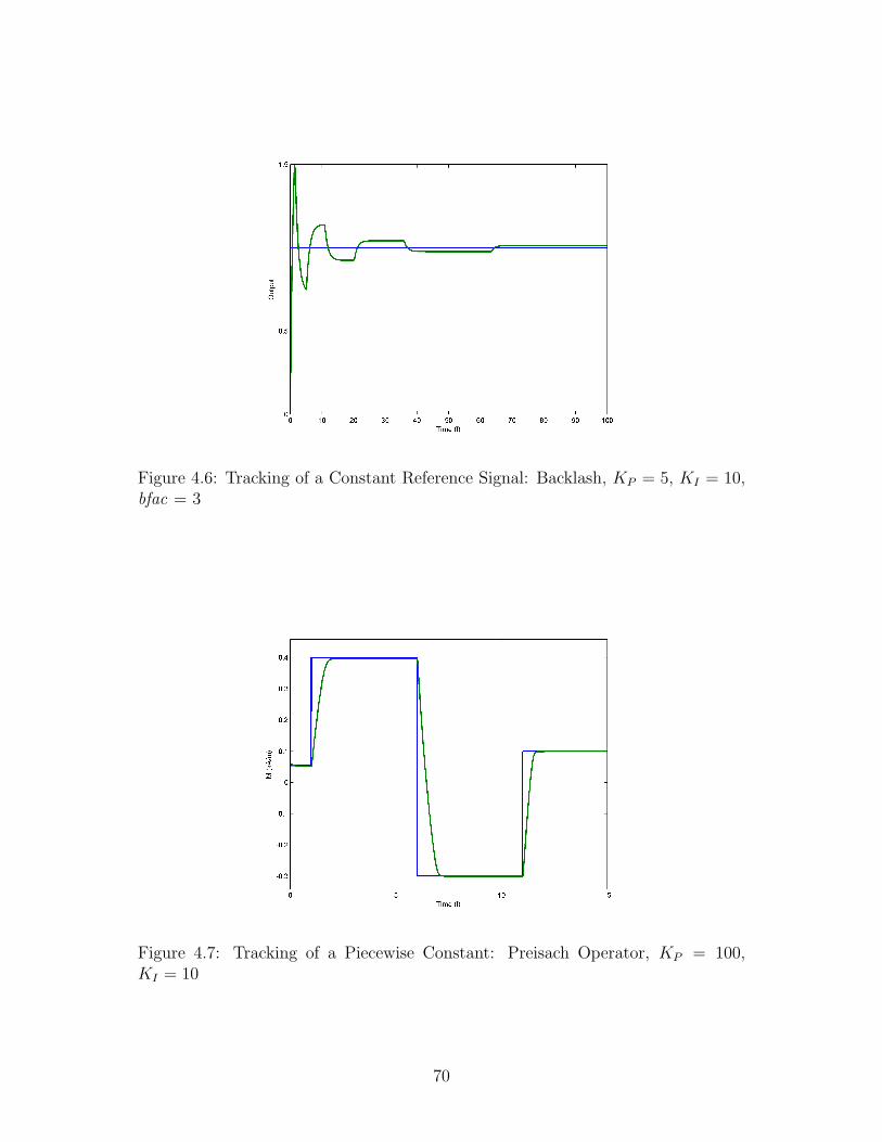
Figure 4.6: Tracking of a Constant Reference Signal: Backlash, KP = 5, KI = 10,bfac = 3
Figure 4.7: Tracking of a Piecewise Constant: Preisach Operator, KP = 100,KI = 10
70

Figure 4.8: Tracking of a Piecewise Ramp Function: Backlash and Elastic PlasticOperators, KP = 10, KI = 5
be seen in Figures 4.10 and 4.11.
71

Figure 4.9: Tracking of a Piecewise Ramp Function: Preisach Operator, KP = 100,KI = 10
Figure 4.10: Tracking of a Sinusoidal Function with Varying Amplitude: Backlashand Elastic Plastic Operators, KP = 20, KI = 10, r(t) = 0.2(5− t) sin(0.4t)
72
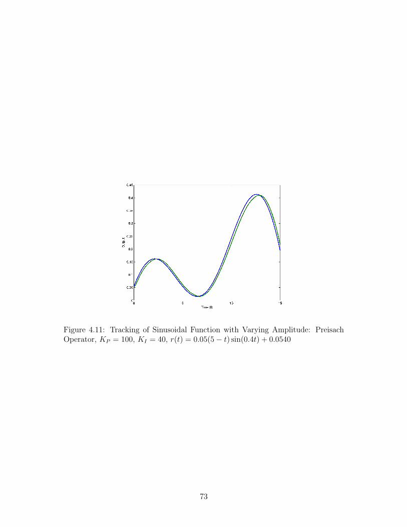
Figure 4.11: Tracking of Sinusoidal Function with Varying Amplitude: PreisachOperator, KP = 100, KI = 40, r(t) = 0.05(5− t) sin(0.4t) + 0.0540
73

Chapter 5
Conclusions and Future Work
In this thesis the control of systems with hysteresis was mathematically investi-gated. A review of hysteresis models was presented including a detailed formu-lation of the Preisach, backlash and elastic-plastic models. An overview of someof the other control methods employed to solve this control problem were discussed.
The control of two similar hysteretic systems has been the focus of this thesis.The first system whose output exhibited hysteretic effects, used a PI controller totrack a reference signal. A BIBO-stability property is shown for continuous signals,and the tracking of a constant signal was shown to be asymptotic. In particular,a bound on the time to reach an arbitrarily small error was found. The originalplant is extended to include a first-order system, and stability is shown for a rangeof parameters. Some simulations were performed on this first-order system.
The second system described the PID control of a second-order system. Theinput to the second-order system was modeled to include hysteresis. The trackingfor a constant reference signal was shown to be asymptotic. The results were thenverified for a first order system. Both systems included hysteresis described by twodifferent sets of assumptions. The assumptions for each of these systems were com-pared, and the assumptions used for the first system was found to be essentially asubset of the those used in the second system.
Possible avenues of future work include extending the results for both systemsto linear systems of arbitrary order. Such an extension would allow for bettermodelling of the actuator. Experimental results suggest that this bound is onlya sufficient condition for stability. Alternative theory could be investigated thatwould guarantee stability and tracking for a larger range of parameters.
74

APPENDICES
75

Appendix A
Proofs and Details
Detailed calculations/details and proofs that were omitted in other sections arepresented here.
A.1 Existence and Uniqueness Proof
The reasoning behind defining the following conditions may not be intuitive, butwill become more apparent in subsequent theorems as to why they were definedin that manner. Logemann breaks his findings into successive theorems, which areeach small steps to the final product. As a result, an existence uniqueness proof willbe provided for a more general system, than that of Theorem 3.5.9. The pertinentsystem is:
x′(t) = (F (u))(t), t > α, (A.1)
x(t) = w(t), t ∈ [0, α], (A.2)
where α ≥ 0 and w ∈ C([0, α]), (if α = 0, then C([0, α]) = R). Assume thatF : C(R+)→ L1
loc(R+) is causal and satisfies (H1) and (H2) where:
(H1) For all a ≥ 0 and v ∈ C([0, a]), there exist δ > 0, γ > 0, and a functionf : [0, γ]→ R+, with f(0) = 0, continuous, such that for all ε ∈ (0, γ].
∫ a+ε
a
|(F (v1))(τ)− (F (v2))(τ)|dτ ≤f(ε) maxτ∈[a,a+ε]
|v1(τ)− v2(τ)|,
for all v1, v2 ∈ C(w; δ, ε)
where B(v; δ, ε) := p ∈ C([0, α + ε]) : p|[0,α] = v, maxt∈[α,α+γ]
|p(t) − v(α)| ≤ δ. This
was defined earlier in Equation (3.23) to be the ε - long extensions of v(t) from α,
76

Figure A.1: Depicting the set B(w; δ, ε)
that are within δ of v(α). This set is depicted in Figure A.1. An element of theset B(v; δ, ε) must be identical to the function v from [0, α] and continuous, within(and including) the boundary of shaded box from (α, α + ε].
The second hypothesis is:
(H2) For all a > 0 and v ∈ C([0, a)), there exists c > 0 such that
∫ t
0
|(F (v))(τ)|dτ ≤ c(1 + maxτ∈[0,t]
|v(τ)|), for all t ∈ [0, a).
The existence and uniqueness claim is as follows:
Lemma A.1.1. For every α ≥ 0 and every w ∈ C([0, α]), there exists a unique so-lution x of (A.1), defined on a maximal interval [0, tmax) with tmax > α. Moreover,if tmax <∞, then
lim supt→tmax
|x(t)| =∞.
Proof. First, existence and uniqueness will be established on a small interval, thenuniqueness will be established on the maximal solution, then finally it will be shownthat if tmax <∞ then the solution becomes unbounded.
Step 1. Existence and uniqueness on a small interval.
77

The aim here is to define an operator that has a fixed point, which is a solutionto Equation (A.1). If the operator is a contraction mapping, then the fixed pointmust be unique, and hence existence and uniqueness can be established on a smallinterval. First, the desired operator, acting on y ∈ C([0, α + ε]) is:
(Γε(y))(t) =
w(t), t ∈ [0, α]
w(α) +∫ tα(F (y))(τ)dτ, t ∈ (α, α + ε],
with the metric d(v1, v2) = maxτ∈[α,α+ε]
|v1(τ)− v2(τ)|. Since the range of the functions
in C(w; δ, ε) on [α, α + ε] is a closed set, then (B(w; δ, ε), d) is a complete metricspace. It remains to show that for small enough ε ∈ (0, γ], Γε acting on B(w; δ, ε)is a contraction map. As a result, the following two properties must be shown.
1) Γε(B(w; δ, ε)) ⊂ B(w; δ, ε).
2) There exists 0 < λ ≤ 1 that for every v1, v2 ∈ B(w; δ, ε),
d(Γε(v1)), (Γε(v2))) ≤ λd(v1, v2).
For the first condition, consider the definition of Γε. Given v ∈ B(w; δ, ε), it isclear that Γε(v) = w on [0, α] and that it is continuous on [0, α + ε]. It remainsto show that for small enough ε, Γε(v) does not escape the δ-bound. Defining thefollowing function facilitates the next calculation.
w(t) =
w(t), t ∈ [0, α]
w(α), t ∈ (α, α + ε].
It is clear that w belongs to B(w; δ, ε). Considering t ∈ [α, α + ε], an estimationyields:
78
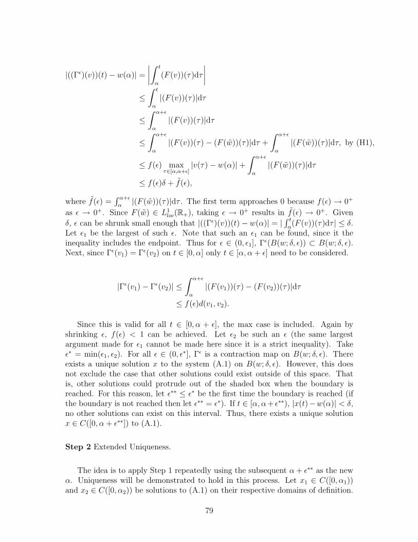
|((Γε)(v))(t)− w(α)| =∣∣∣∣∫ t
α
(F (v))(τ)dτ
∣∣∣∣≤∫ t
α
|(F (v))(τ)|dτ
≤∫ α+ε
α
|(F (v))(τ)|dτ
≤∫ α+ε
α
|(F (v))(τ)− (F (w))(τ)|dτ +
∫ α+ε
α
|(F (w))(τ)|dτ, by (H1),
≤ f(ε) maxτ∈[α,α+ε]
|v(τ)− w(α)|+∫ α+ε
α
|(F (w))(τ)|dτ
≤ f(ε)δ + f(ε),
where f(ε) =∫ α+ε
α|(F (w))(τ)|dτ . The first term approaches 0 because f(ε) → 0+
as ε → 0+. Since F (w) ∈ L1loc(R+), taking ε → 0+ results in f(ε) → 0+. Given
δ, ε can be shrunk small enough that |((Γε)(v))(t)− w(α)| = |∫ tα(F (v))(τ)dτ | ≤ δ.
Let ε1 be the largest of such ε. Note that such an ε1 can be found, since it theinequality includes the endpoint. Thus for ε ∈ (0, ε1], Γε(B(w; δ, ε)) ⊂ B(w; δ, ε).Next, since Γε(v1) = Γε(v2) on t ∈ [0, α] only t ∈ [α, α + ε] need to be considered.
|Γε(v1)− Γε(v2)| ≤∫ α+ε
α
|(F (v1))(τ)− (F (v2))(τ)|dτ
≤ f(ε)d(v1, v2).
Since this is valid for all t ∈ [0, α + ε], the max case is included. Again byshrinking ε, f(ε) < 1 can be achieved. Let ε2 be such an ε (the same largestargument made for ε1 cannot be made here since it is a strict inequality). Takeε∗ = min(ε1, ε2). For all ε ∈ (0, ε∗], Γε is a contraction map on B(w; δ, ε). Thereexists a unique solution x to the system (A.1) on B(w; δ, ε). However, this doesnot exclude the case that other solutions could exist outside of this space. Thatis, other solutions could protrude out of the shaded box when the boundary isreached. For this reason, let ε∗∗ ≤ ε∗ be the first time the boundary is reached (ifthe boundary is not reached then let ε∗∗ = ε∗). If t ∈ [α, α+ ε∗∗), |x(t)−w(α)| < δ,no other solutions can exist on this interval. Thus, there exists a unique solutionx ∈ C([0, α + ε∗∗]) to (A.1).
Step 2 Extended Uniqueness.
The idea is to apply Step 1 repeatedly using the subsequent α+ ε∗∗ as the newα. Uniqueness will be demonstrated to hold in this process. Let x1 ∈ C([0, α1))and x2 ∈ C([0, α2)) be solutions to (A.1) on their respective domains of definition.
79
Let β := minα1, α2. Claim that x1 = x2 on [0, β). Seeking a contradiction, define:
α∗ := inft ∈ [0, β) : x1(t) 6= x2(t) < β,
That is, α∗ is the last point on which the functions x1, x2 are equal. Letx(t) = x1(t) = x2(t) on [0, α∗]. Apply Step 1 again on α∗, so that there existsε such that 0 < ε < β−α∗, where there exists a unique solution x on C([0, α∗+ ε]),contradicting the definition of α∗.
Step 3 Existence of a maximal solution.
If Steps 1 and 2 are applied successively, then a unique maximal solution isobtained. Formally, let T be the set of all τ > α s.t. there exists a solution xτ
to (A.1) on the interval [0, τ). From Step 1, T 6= 0. Let tmax := sup T and definex : [0, tmax) → R by setting x(t) = xτ (t) for t ∈ [0, τ) where τ ∈ T. Since thisapplies to all τ ∈ T, then this is the maximal solution of (A.1). Uniqueness followsfrom Step 2.
Step 4 If tmax <∞, x is unbounded.
This is the last claim of Lemma A.1.1. It will be shown via a contrapositiveproof. Consider x bounded on [0, t1) where t1 <∞. Integrating A.1 yields:
x(t) = x(α) +∫ tα(F (x))(τ)dτ, for all t ∈ [α, t1)
By(H2), there exists c > 0 such that,
∫ t
α
|(F (x))(τ)|dτ ≤ c(1 + supτ∈[0,t1]
|x(τ)|) <∞,
so F (x) ∈ L1([0, t1]), and limt→t1
x(t) exists and is finite. Step 1 can be applied.
However, since t1 was arbitarily chosen, this argument works for all t1 ∈ (0,∞).Therefore tmax =∞.
A.2 Showing (3.25) satisfies Lemma A.1
The system in (3.25) will be shown to satisfy (H1) and (H2), and that there isno finite escape time (that is from Lemma A.1, x must be bounded locally). LetF : C(R+)→ L1
loc(R+) be defined by
80
F (v) := κ(ρ− η − (G Φ)(v))
To show that F satisfies (H1). Let a ≥ 0, and v ∈ C([0, a]).∫ a+ε
a
|(F (v1))(τ)− (F (v2))(τ)|dτ =
∫ a+ε
a
|κ(t)(G(Φ(v1)− Φ(v2)))(τ)|dτ
≤ ‖κ‖L∞(R+)
∫ a+ε
a
|κ(t)(G(Φ(v1)− Φ(v2)))(τ)|dτ
by Holder’s inequality, using the function itself 1
≤√ε ‖κ‖L∞(R+) ‖G‖ ‖(Φ(v1)− Φ(v2))‖L2([a,a+ε])
≤ ε ‖κ‖L∞(R+) ‖G‖ ‖(Φ(v1)− Φ(v2))‖C([a,a+ε]) , by (N3)
≤ ελ1 ‖κ‖L∞(R+) ‖G‖ ‖(v1 − v2)‖C([a,a+ε])
Assumption (H1) holds with
f(ε) := ελ1 ‖κ‖L∞(R+) ‖G‖.
To establish (H2), let a > 0, v ∈ C([0, a)). For t ∈ [0, a),
∫ t
0
|(F (v))(τ)|dτ ≤ ‖κ‖L∞(R+)
∫ t
0
|ρ− η(τ)− ((G Φ)(v))(τ)|dτ,
≤ ‖κ‖L∞(R+) [ρt+
∫ t
0
|η(τ)|dτ +
∫ t
0
|(G(Φ(v)))(τ)|dτ ],
≤ ‖κ‖L∞(R+) [ρa+
∫ a
0
|η(τ)|dτ +
∫ t
0
|(G(Φ(v)))(τ)|dτ ].
Considering only the last term:
∫ t
0
|(G(Φ(v)))(τ)|dτ = ‖G(Φ(v)) · 1‖L1[0,t]
, using Holder’s inequality
≤ ‖G(Φ(v))‖L2[0,t]‖1‖L2
[0,t]
≤√t
(∫ t
0
|(G(Φ(v)))(τ)|2dτ
) 12
,
taking the supremum and factoring out the terms of the integral,
≤ t ‖G‖ maxτ∈[0,t]
|(Φ(v))(τ)|, by (N4) and t ≤ a,
≤ a ‖G‖ β(1 + maxτ∈[0,t]
|v(τ)|)
81
Since maxτ∈[0,t]
|v(τ)| > 0, from the above two sets of inequalities:
∫ t
0
|(F (v))(τ)|dτ ≤ ‖κ‖L∞(R+) [ρa+
∫ a
0
|η(τ)|dτ + a ‖G‖ β(1 + maxτ∈[0,t]
|v(τ)|)],
≤ ‖κ‖L∞(R+) [ρa+
∫ a
0
|η(τ)|dτ + a ‖G‖ β] · (1 + maxτ∈[0,t]
|v(τ)|).
The operator F satisfies (H2) with
c := ‖κ‖L∞(R+) [ρa+∫ a
0|η(τ)|dτ + a ‖G‖ β].
There exists a unique solution x to A.1 defined on a maximal interval [0, tmax).It remains to show that x does not have finite escape time, that is, x is boundedlocally. Let t1 > 0 be an arbitrary time. Integrating (3.25) for t ∈ [0, t1) yields:
x(t) = x(0) +
∫ t
0
[κ(τ)(ρ− η(τ) + (G(Φ(x)))(τ))]dτ .
However, the bound on maxσ∈[0,t]
|x(σ)| will be considered in place of the usual |x(t)|.
This will be more useful since (N4) yields x back in this form, and the proof relieson an application of Gronwall’s Lemma. Making an estimate using the same toolsas seen previously in this proof:
maxσ∈[0,t]
|x(σ)| ≤ |x(0)|+‖κ‖L∞(R+) [ρt+
∫ t
0
|η(τ)|dτ+
∫ t
0
|(G(Φ(u)))(τ)|dτ ], for all t ∈ [0, t1).
(A.3)
Estimating the last term (and applying (N4) in the second last step) yields:
∫ t
0
|(G(Φ(x)))(τ)|dτ ≤√t
(∫ t
0
|(G(Φ(x)))(τ)|2dτ
) 12
,
≤√t1 ‖G‖
(∫ t
0
maxσ∈[0,τ ]
|(Φ(x))(σ)|2dτ
)1/2
≤√t1 ‖G‖
(∫ t1
0
maxσ∈[0,τ ]
(1 + |x(σ)|)2dτ
)1/2
≤√
2t1 ‖G‖(∫ t1
0
maxσ∈[0,τ ]
(1 + |x(σ)|2)dτ
)1/2
.
82
The last step used the inequality 2a2 +2b2 ≥ (a+b)2 +(a−b)2 ≥ (a+b)2. Next,let x(t) := max
σ∈[0,t]|x(σ)|. Since t1 is fixed, there exists constants β1 and β2 (simply
by equating components) such that
x(t) ≤ β1 + β2
(∫ t
0
(1 + (x2(τ)))dτ
)1/2
.
Thus,
x2(t) ≤
(β1 + β2
(∫ t
0
(1 + x2(τ))dτ
)1/2)
≤ 2β21 + 2β2
2
(∫ t
0
(1 + x2(τ))dτ
)≤ 2β2
1 + 2β22t1 + 2β2
2
∫ t
0
x2(τ)dτ, for all t ∈ [0, t1).
Applying Gronwall’s Lemma:
x2(t) ≤ (2β21 + 2β2
2t1) exp (2β22t1), for all t ∈ [0, t1).
But since t1 was chosen arbitrarily, this argument holds for t1 ∈ (0,∞), so x isbounded locally. Hence x does not have finite escape time.
A.3 Leibniz’s Rule for Convolution Differentia-
tion
Here, Leibniz’s integral rule will be applied to the differentiation of a convolution.Let g and h be functions defined on the right-half real line, and let f(τ, t) =g(τ)h(t− τ).
d
dt(g(t) ? h(t))
=d
dt
(∫ t
0
g(τ)h(t− τ)dτ
)=d
dt
(∫ t
0
f(τ, t)dτ
)
Leibniz’s rule states:
83

∂
∂z
∫ b(z)
a(z)
f(x, z)dx =
∫ b(z)
a(z)
∂f
∂zdx+ f(b(z), z)
∂b
∂z− f(a(z), z)
∂a
∂z,
so from above:
d
dt(g(t) ? h(t))
=f(t, t) + 0 +
∫ t
0
g(τ)h′(t− τ)dτ
=g(t)h(0) + g(t) ? h′(t)
=g(t) ? h(0)δ0 + g(t) ? h′(t)
but since convolution is commutative:
d
dt(g(t) ? h(t))
=d
dt(h(t) ? g(t))
=h(t) ? g(0)δ0 + h(t) ? g′(t)
A.4 Left Half Complex Plane Poles → Exponen-
tially Decaying Functions
A brief justification of the poles of a second-order transfer function having negativereal part→ exponentially decays is given here. This result can be readily extendedto higher order systems. It can be verified that:
h(s) =1
ms2 + cs+ k.
Note that the coefficients of the polynomial in the denominator of h(s) are real.The transfer function of ρ has the same denominator, so the exact same argumentcan be applied. This implies that the roots of p(s) := ms2 + cs+ k are either real,or occur in complex conjugates. By the fundamental theorem of algebra, h(s) canbe written as:
h(s) =1m
(s− a1)(s− a2),
where in general a1, a2 ∈ C. Since p(s) is a second degree real coefficient polynomial,either the roots are both strictly real, or are complex conjugates. Suppose all ofa1, a2 are real. Then there exists a unique partial fraction decomposition, such that:
84

h(s) =A1
s− a1
+A2
s− a2
such that A1, A2 ∈ R. By linearity of the Laplace transform, h(t) is the sum of theinverse Laplace transforms of each of the terms above.
L−1(h(s)) = h(t) = A1ea1t + A2e
a2t
Knowing that a1, a2 < 0 it is clear that h exponentially decays as t→∞. Con-sider the other case, where a1, a2 are complex conjugates. Hence, the polynomial(s− a1)(s− a2) = (s2 − (a1 + a2)s + a1a2) would have real coefficients. Again, bypartial fraction decomposition, there exists a unique B1, B2 ∈ R such that
h(s) =B1s+B2
s2 − (a1 + a2)s+ a1a2
,
whose inverse Laplace transform would be h(t) = f(t)eRe(a1)t, where f(t) is abounded oscillatory function (a sum of sine and cosine functions). Again by theHurwitz condition, Re(ai) < 0 for i = 1, 2, therefore h exponentially decays ast → ∞. Therefore if the poles of h(s) are Hurwitz, then h decays exponentiallyand hence h ∈ L2
α(R+). Because of the form of h, any linear combination of itsderivatives must also be exponentially decaying.
85

Appendix B
MATLAB R© Code
The code used to produce the simulations will be presented here. The following isthe code used for the backlash model.
function [y,binc] = backlashfast(u1,u2,u3,curbinc,bfac)
%u1 = present u, u2 = u one time step ago,
%u3 = u one time step before u2
%Initial operator value.
y = bh(bfac,u1,curbinc);
if sign(u1-u2) ~= sign(u2-u3)
binc = y;
else
binc = curbinc;
end
%When u ceases to be monotone,
%the next subinterval in the partition
%begins.
end
function output = bh(h,v,w)
output = max(v-h,min(v+h,w));
%Defines the bh function needed to define the backlash operator.
end
The elastic-plastic operator is defined similarly.
86

%Defined structurally the same as the fast backlash operator.
function [y,einc,uinc] =...
elasticplasticfast(u1,u2,u3,cureinc,curuinc,efac)
y = eh(efac,u1 - curuinc + cureinc);
if sign(u1-u2) ~= sign(u2-u3)
einc = y;
uinc = u1;
else
einc = cureinc;
uinc = curuinc;
end
function output = eh(h,u)
output = min(h,max(-h,u));
end
The Preisach model required several functions. The function buildlinesegmentsidentified the locations of all the line segments that form the boundary. The func-tion findbound found all the relevant points that make up the boundary from agiven input.
function [v,boundaryout] =...
preisachtestweight(u,usat,boundaryin,weight)
%v,boundaryout
%a is the distance from the bottom of the
%cell to where the boundary is
%b is 1 if a had to be modified
%(i.e. the rounding function put a and the
%boundary in two different cells)
%c is a fix in the case of boundary = usat, or -usat
%initialize plane
gridsize = 0.5;
%note, gridsize must divide usat
%(i.e. usat/gridsize must be a natural number)
relsize = round(usat/gridsize);
plane = zeros(relsize*2,relsize);
for i=1:1:relsize
87

for j=1:1:i
plane(i,j) = -1;
plane(relsize*2-i+1,j) = 1;
end
plane(i,i) = -0.5;
plane(relsize*2-i+1,i)=0.5;
end
if abs(u(end)) < usat
%initialize weighting
%if new corner emerges, or a corner is erased....
if size(boundaryin,2)>1
if sign(boundaryin(end) - boundaryin(end-1)) ~=...
sign(u(end) - boundaryin(end)) || abs(u(end)) >= abs(boundaryin(end-1))
boundary = findbound(u,usat);
else
boundary = [boundaryin(1:end-1),u(end)];
end
else
boundary(1) = min(usat,max(-usat,u(end)));
if size(u,2) > 1
boundary(1) = min(usat,max(-usat,u(end-1)));
end
if sign(boundary(1))==...
-sign(u(end)-boundary(1)) && abs(boundary(1))~=usat
boundary(2) = u(end);
end
end
lineseg = buildlinesegments(boundary);
a=0;
b=0;
c=0;
boundaryout = boundary;
%offset for boundary
if abs(boundary) == usat
c = 1;
end
%Start editing the plane:
%cls for current line segment
corners = zeros(size(plane));
for cls = 0:1:size(lineseg,1) - 1
88
%LOCATE CORNERS
if lineseg(end-cls,3)/gridsize ~=...
floor(lineseg(end-cls,3)/gridsize)
locy = relsize - floor(lineseg(end-cls,4)/gridsize);
locx = floor(lineseg(end-cls,3)/gridsize)+1;
corners(locy,locx) = corners(locy,locx) + 1;
end
end
for cls = 0:1:size(lineseg,1) - 1
%find the sign of y2-y1
incdec = sign(lineseg(end-cls,4)-lineseg(end-cls,2));
%if there is no change, then the boundary is complete
%(i.e. we’ve hit the
%0 slope part of the boundary, note that this might not always occur
if incdec == 0
if a~=1 && a~=0
if term == 1
plane(starty-i+b,stopx) = 2*a - a^2;
else
plane(starty+i-b,stopx) = a^2 - 1;
end
end
break
end
%
diffx = lineseg(end-cls,1)/gridsize -...
floor(lineseg(end-cls,1)/gridsize);
b = 0;
%Consider two seperate cases,
%where xmin does not fall on an edge of the
%cell, and one that does
if diffx ==0
%xmin touches the edge of a cell
a = (lineseg(end-cls,2))/gridsize - ...
floor((lineseg(end-cls,2))/gridsize);
else
%xmin does not touch the edge of a cell
a = -incdec*diffx + (lineseg(end-cls,2))/gridsize -...
floor(lineseg(end-cls,2)/gridsize);
end
89

if a > 1;
a = a-1;
b = 1;
end
if a < 0;
a = a + 1;
b=1;
end
%y2-y1 < 0
if incdec == -1
startx = floor(lineseg(end-cls,1)/gridsize) + 1;
stopx = floor(lineseg(end-cls,3)/gridsize) + 1;
starty = relsize - floor(lineseg(end-cls,2)/gridsize);
stopy = relsize - floor(lineseg(end-cls,4)/gridsize);
%Build the in between points to the corners
for i = 1+ceil(diffx):1:stopx-startx
plane(starty + i -1 - b+c,startx + i - 1) = a^2 - 1;
plane(starty + i -b,startx + i -1) = 2*a-a^2;
%Rewrite cells:
if starty+i-1-b > relsize + 1
for j = 1:1:starty+i-1-b - relsize
plane(starty + i - 1 - b - j, startx + i - 1) = -1;
end
end
if starty+i-1-b < relsize - 1
for j = 1:1:relsize - (starty+i-1-b) - 1
plane(starty + i - b + j, startx + i - 1) = 1;
end
end
end
%Corners: (can only handle 1 per cell, for now...)
if lineseg(end-cls,3)/gridsize -...
floor(lineseg(end-cls,3)/gridsize)~=...
0 && lineseg(end-cls,4) - lineseg(end-cls-1,4) ~=0
diffx1 = lineseg(end-cls,3)/gridsize -...
floor(lineseg(end-cls,3)/gridsize);
diffx2 = ceil(lineseg(end-cls,3)/gridsize) -...
lineseg(end-cls,3)/gridsize;
%oa and ob determine the cells in the same column
%as the corner cell
%that need to be changed
90

oa = 0; ob = 0;
if ceil(lineseg(end-cls,4)/gridsize) -...
lineseg(end-cls,4)/gridsize - diffx1 >= 0
a1 = ceil(lineseg(end-cls,4)/gridsize) -...
lineseg(end-cls,4)/gridsize - diffx1;
a2 = ceil(lineseg(end-cls,4)/gridsize) -...
lineseg(end-cls,4)/gridsize;
b1 = a2;
if ceil(lineseg(end-cls,4)/gridsize) -...
lineseg(end-cls,4)/gridsize - diffx2 >= 0
b2 = ceil(lineseg(end-cls,4)/gridsize) -...
lineseg(end-cls,4)/gridsize - diffx2;
else
b2 = 0; ob = 1;
diffx2 = b1;
end
else
a1 = 0; oa = 1;
a2 = ceil(lineseg(end-cls,4)/gridsize) -...
lineseg(end-cls,4)/gridsize;
diffx1 = a2;
b1 = a2;
if ceil(lineseg(end-cls,4)/gridsize) -...
lineseg(end-cls,4)/gridsize - diffx2 >= 0
b2 = ceil(lineseg(end-cls,4)/gridsize) -...
lineseg(end-cls,4)/gridsize - diffx2;
else
b2 = 0; ob = 1;
diffx2 = b1;
end
end
negarea = (a1 + a2)/2*diffx1 + (b1 + b2)/2*diffx2;
plane(stopy,stopx) = 1 - 2*negarea;
if stopy ==1
plane(stopy, stopx) = (oa*(1 -(ceil(lineseg(end-cls,3)/gridsize) -...
lineseg(end-cls,3)/gridsize) -diffx1)^2 + ob*(1-...
(lineseg(end-cls,3)/gridsize -...
floor(lineseg(end-cls,3)/gridsize)) - diffx2)^2) - 1;
else
plane(stopy-1,stopx)=(oa*(1-(ceil(lineseg(end-cls,3)/gridsize)-...
lineseg(end-cls,3)/gridsize) -diffx1)^2 + ob*(1-...
(lineseg(end-cls,3)/gridsize -...
floor(lineseg(end-cls,3)/gridsize)) - diffx2)^2) - 1;
91
end
if stopy-1-b > relsize + 1
for j = 1:1:stopy-1-b - relsize
plane(stopy - j - 1, stopx) = -1;
end
end
if stopy-1-b < relsize - 1
for j = 1:1:relsize - (stopy-1-b) - 1
plane(stopy + j, stopx) = 1;
end
end
end
end
%y2-y1 > 0
if incdec == 1
startx = floor(lineseg(end-cls,1)/gridsize) + 1;
stopx = floor(lineseg(end-cls,3)/gridsize) + 1;
starty = relsize - floor(lineseg(end-cls,2)/gridsize);
stopy = relsize - floor(lineseg(end-cls,4)/gridsize);
%Build the in between points to the corners
for i = 1+ceil(diffx):1:stopx-startx
plane(starty - i + b,startx + i - 1) = a^2-1;
plane(starty + 1 - i + b, startx + i - 1) = 2*a - a^2;
%Rewrite cells:
if starty-i + b > relsize + 1
for j = 1:1:starty-i+b-relsize
plane(starty - i + b - j, startx + i - 1) = -1;
end
end
if starty-i+b < relsize
for j = 1:1:relsize-(starty-i+b)-1
plane(starty - i + b + j + 1, startx + i - 1) = 1;
end
end
end
%Corners: (can only handle 1 per cell, for now...)
if lineseg(end-cls,3)/gridsize -...
floor(lineseg(end-cls,3)/gridsize)~=...
0 && lineseg(end-cls,4) - lineseg(end-cls-1,4) ~=0
92
diffx1 = lineseg(end-cls,3)/gridsize -...
floor(lineseg(end-cls,3)/gridsize);
diffx2 = ceil(lineseg(end-cls,3)/gridsize) -...
lineseg(end-cls,3)/gridsize;
%oa and ob determine the cells
%in the same column as the corner cell
%that need to be changed
oa = 0; ob = 0;
if lineseg(end-cls,4)/gridsize -...
floor(lineseg(end-cls)/gridsize) - diffx1 >= 0
a1 = lineseg(end-cls,4)/gridsize - diffx1 -...
floor(lineseg(end-cls,4)/gridsize);
a2 = lineseg(end-cls,4)/gridsize -...
floor(lineseg(end-cls,4)/gridsize);
b1 = a2;
if lineseg(end-cls,4)/gridsize -...
floor(lineseg(end-cls,4)/gridsize) - diffx2 >= 0
b2 = lineseg(end-cls,4)/gridsize - diffx2 -...
floor(lineseg(end-cls,4)/gridsize);
else
b2 = 0; ob = 1;
diffx2 = b1;
end
else
a1 = 0; oa = 1;
a2 = lineseg(end-cls,4)/gridsize -...
floor(lineseg(end-cls,4)/gridsize);
diffx1 = a2;
b1 = a2;
if lineseg(end-cls,4)/gridsize -...
floor(lineseg(end-cls,4)/gridsize) - diffx2 >= 0
b2 = lineseg(end-cls,4)/gridsize - diffx2 -...
floor(lineseg(end-cls,4)/gridsize);
else
b2 = 0; ob = 1;
diffx2 = b1;
end
end
posarea = (a1 + a2)/2*diffx1 + (b1 + b2)/2*diffx2;
plane(stopy,stopx) = 2*posarea - 1;
if stopy == size(plane,1)
plane(stopy,stopx) = 1-...
(oa*(1-(ceil(lineseg(end-cls,3)/gridsize) -...
93

lineseg(end-cls,3)/gridsize) -diffx1)^2 + ob*(1-...
(lineseg(end-cls,3)/gridsize -...
floor(lineseg(end-cls,3)/gridsize)) - diffx2)^2);
else
plane(stopy+1,stopx) = 1-...
(oa*(1-(ceil(lineseg(end-cls,3)/gridsize)-...
lineseg(end-cls,3)/gridsize) -diffx1)^2 + ob*(1-...
(lineseg(end-cls,3)/gridsize -...
floor(lineseg(end-cls,3)/gridsize)) - diffx2)^2);
end
if stopy-1-b > relsize + 1
for j = 1:1:stopy-1-b - relsize
plane(stopy - j, stopx) = -1;
end
end
if stopy-1-b < relsize - 1
for j = 1:1:relsize - (stopy-1-b) - 1
plane(stopy + j + 1, stopx) = 1;
end
end
end
end
term = incdec;
end
%Fix the borders
for i = 1:1:usat/gridsize
if plane(i,i)<=-1
plane(i,i) = -0.5;
end
if 0<=plane(i+1,i) && plane(i,i)~=-0.5
plane(i,i) = plane(i,i) + 0.5;
if i > 1
plane(i-1,i) = 0;
end
end
if corners(i,i)~=0 && plane(i,i) <=0
plane(i,i) = plane(i,i)+ 0.5;
end
94

if plane(end-i+1,i) >=1
plane(end-i+1,i) = 0.5;
end
if 0>= plane(end-i,i) && plane(end-i+1,i)~= 0.5
plane(end-i+1,i) = plane(end-i+1,i) -0.5;
if i > 1
plane(end-i+2,i) = 0;
end
end
v = sum(sum(plane.*weight));
end
else
v = sum(sum(weight))*sign(u(end));
boundary(1) = usat*sign(u(end));
boundaryout = boundary;
end
function boundary = findbound(u,usat)
%Finds the information necessary for the Preisach boundary
[val,ind] = max(abs(u));
if val > usat
boundary(1) = usat*sign(u(ind));
else
boundary(1) = sign(u(ind))*val;
end
minmax = sign(u(ind));
unew = u(ind:end);
k=2;
while max(size(unew))>1
if minmax == 1
[val,ind] = min(unew);
if abs(val) > usat
boundary(k) = -usat;
else
boundary(k) = val;
end
k=k+1;
unew = unew(ind:end);
minmax=minmax*-1;
end
95
if minmax== -1
[val,ind]=max(unew);
if abs(val) > usat
boundary(k) = usat;
else
boundary(k) = val;
end
k=k+1;
unew = unew(ind:end);
minmax=minmax*-1;
end
if size(unew,2) > 1
if unew(1) == unew(2)
unew = unew(2:end);
k = k-1;
end
end
end
if size(boundary,2)>1
if boundary(end)==boundary(end-1)
boundary = boundary(1:end-1);
end
end
end
function lineseg = buildlinesegments(boundary)
%lineseg is a matrix carrying details about the line segments:
%column 1: xmin, column 2: y at xmin, column 3: xmax,
%column 4: y at xmax
%initialize the line segments:
lineseg = zeros(size(boundary,2),4);
lineseg(1,1) = 0;
lineseg(1,2) = 0;
lineseg(1,3) = 10;
lineseg(1,4) = 0;
%The first two lines don’t satisfy
%the "-1", "+1" properties since they
%deal with the 0 boundary
lineseg(2,1) = 0;
lineseg(2,2) = boundary(1);
lineseg(2,3) = abs(boundary(1));
lineseg(2,4) = 0;
96
lineseg(1,1) = lineseg(2,3);
lineseg(1,2) = lineseg(2,4);
for i = 3:1:size(boundary,2)+1
%Build line segment matrix according to boundary
%See Drawings
lineseg(i,1) = 0;
lineseg(i,2) = boundary(i-1);
if boundary(i-1)-boundary(i-2)>0
%Increasing
lineseg(i,3) = (lineseg(i-1,3) -...
lineseg(i-1,4) + lineseg(i,2))/2;
lineseg(i,4) = (lineseg(i-1,4) -...
lineseg(i-1,3) + lineseg(i,2))/2;
else
%Decreasing
lineseg(i,3) = (lineseg(i-1,4) +...
lineseg(i-1,3) - lineseg(i,2))/2;
lineseg(i,4) = (lineseg(i-1,4) +...
lineseg(i-1,3) + lineseg(i,2))/2;
end
for j=i:-1:2
lineseg(j-1,1)=lineseg(j,3);
lineseg(j-1,2)=lineseg(j,4);
end
end
check = 0;
i=1;
while check ~=1
if lineseg(i,1) ==lineseg(i,3)
lineseg = [lineseg(1:i-1,:);lineseg(i+1:end,:)];
i = i-1;
end
if i == size(lineseg,1)
check = 1;
end
i=i+1;
end
The procedure that ran the ode4 Runge-Kutta solver was identical for all threehysteresis operators. Only the code for the backlash operator is presented here.Running the code for thee other operators would simply require a change in eachplace the backlash function is called and the inputs to each function.
97

function [time,y] = ...
ode4backlashfast(Kp,Ki,M,sigma,h,timesteps,bfac,Xi,r)
y = zeros(1,timesteps);
y(1) = 0;
y(2) = 0;
u = zeros(1,timesteps);
u(1) = 0;
u(2) = 0;
e = zeros(1,timesteps);
e(1) = r(0) - y(1);
e(2) = r(h) - y(2);
v = zeros(1,timesteps);
time = 0:h:h*timesteps-h;
t = 0;
curbinc = Xi;
epsilon = 0.001;
cumerror = h*(e(1) + e(2))/2;
k1 = M*bh(bfac,Kp*r(0),Xi);
k2 = -sigma*(0.5*h*k1) + M*bh(bfac,Kp*(r(0.5*h) - 0.5*k1*h) +...
Ki*(0.25*h*(r(0.5*h) + r(0) - 0.5*h*k1)),Xi);
k3 = -sigma*(0.5*h*k2) + M*bh(bfac,Kp*(r(0.5*h) - 0.5*k2*h) +...
Ki*(0.25*h*(r(0.5*h) + r(0) - 0.5*h*k1)),Xi);
k4 = -sigma*(h*k3) + M*bh(bfac,Kp*(r(h) - h*k3) +...
Ki*0.5*(r(0.5*h) + r(0) - h*k1),Xi);
for i=3:1:timesteps
y(i) = y(i-1) + h*(k1+2*k2+2*k3+k4)/6;
e(i) = r(t) - y(i);
cumerror = cumerror + h*(exp(epsilon*t)*e(i) +...
exp(epsilon*(t-h))*e(i-1))/2;
u(i) = Kp*(e(i)) + Ki*exp(epsilon*-t)*cumerror;
k1 = -sigma*y(i) +...
M*backlashfast(u(i),u(i-1),u(i-2),curbinc,bfac);
u(i) = Kp*(r(t+0.5*h) - y(i) - 0.5*k1*h) + ...
Ki*exp(-epsilon*(t+0.5*h))*(cumerror + ...
0.25*h*(exp(epsilon*(t+0.5*h))*(r(t+0.5*h) ...
- y(i) -0.5*h*k1)+exp(epsilon*t)*(r(t) - y(i))));
k2 = -sigma*(y(i) + 0.5*k1*h) +...
M*backlashfast(u(i),u(i-1),u(i-2),curbinc,bfac);
u(i) = Kp*(r(t+0.5*h) - y(i) - 0.5*k2*h) +...
Ki*exp(-epsilon*(t+0.5*h))*(cumerror +...
0.25*h*(exp(epsilon*...
(t+0.5*h))*(r(t+0.5*h) - y(i)-...
98

0.5*h*k1)+exp(epsilon*t)*(r(t) - y(i))));
k3 = -sigma*(y(i) + 0.5*k2*h) +...
M*backlashfast(u(i),u(i-1),u(i-2),curbinc,bfac);
u(i) = Kp*(r(t+h) - y(i) - h*k3) +...
Ki*exp(-epsilon*(t+h))*(cumerror +...
0.5*h*(exp(epsilon*(t+h))*(r(t+h) - y(i) -h*k1)+...
exp(epsilon*t)*(r(t) - y(i))));
k4 = -sigma*(y(i) + k3*h) +...
M*backlashfast(u(i),u(i-1),u(i-2),curbinc,bfac);
%Rewrite u(i) to be what we expected it to be originally
u(i) = Kp*e(i) + Ki*exp(epsilon*-t)*cumerror;
[void,binc] = backlashfast(u(i),u(i-1),u(i-2),curbinc,bfac);
curbinc = binc;
v(i-1) = backlashfast(u(i),u(i-1),u(i-2),curbinc,bfac);
t = t+h;
%i
end
v(i) = backlashfast(u(i),u(i-1),u(i-2),curbinc,bfac);
y(end) = y(end-1) + h*(k1+2*k2+2*k3+k4)/6;
99
References
[1] K.K. Ahn and N.B. Kha. Modeling and control of shape memory alloy actu-ators using Preisach model, genetic algorithm and fuzzy logic. Mechatronics,18:141–152, 2008. 23
[2] F. Bagagiolo. Dynamic programming for some optimal control problems withhysteresis. Nonlinear Differential Equations and Applications NoDEA, 9:149–174, 2002. 60
[3] F. Bagagiolo. Viscosity solutions for an optimal control problem with Preisachhysteresis nonlinearities. ESAIM: Control, Optimization and Calculus of Vari-ations, 10:271–294, 2004. 60
[4] M. Brokate and J. Sprekels. Phase transitions and hysteresis. Springer-Verlag,1994. 4, 8, 13, 18, 23, 24, 25
[5] G.S. Choi, Y.A. Lim, and G.H. Choi. Tracking position control of piezoelectricactuators for periodic reference inputs. Mechatronics, 12:669–684, 2002. 23
[6] M.L. Corradini, G. Orlando, and G. Parlangeli. A VSC (variable structurecontrol) approach for the robust stabilization of nonlinear plants with uncertainnonsmooth actuator nonlinearities - a unified framework. IEEE Transactionson Automatic Control, 54:807 – 813, 2004.
[7] R. Curtain, H. Logemann, and O. Staffans. Stability results of Popov-typefor infinite-dimensional systems with applications to integral control. Proc.London Math. Soc., 86:779–816, 2003.
[8] R. Curtain and H. Zwart. An Introduction to Infinite-Dimensional LinearSystems Theory. Springer, 1995. 21, 22, 50, 51
[9] C.A. Desoer and M. Vidyasagar. Feedback Systems: Input-Output Properties.Academic Press, 1975. 21, 35, 36, 37, 51
[10] D. Flynn, H. McNamara, P. OKane, and A. Pokrovskii. Application of thePreisach model in soil-moisture hysteresis. Preprint.
[11] R. Gorbet. Control of Hysteresis systems with Preisach Representations. PhDthesis, University of Waterloo, 1997. 8
100
[12] R. Gorbet, K. Morris, and D. Wang. Passivity-based stability and control ofhysteresis in smartactuators. IEEE Transactions on Control Systems Technol-ogy, 9:5–16, January 2001. 8
[13] A. Hatch, R. Smith, and T. De. Model development and control design forhigh speed atomic force microscopy. SPIE Conference, San Diego, 2004. 62
[14] C. Hu and X. Zhang. Closed-loop control system of piezoceramic actuatorswith improved Preisach model. Proceedings of the 7th World Congress onIntelligent Control and Automation, pages 7385 – 7388, 2008. 23, 62
[15] F. Ikhouane, V. Maosa, and J. Rodellar. Adaptive control of a hystereticstructural system. Automatica, 41:225–231, 2005. 62
[16] F. Ikhouane and J. Rodellar. A linear controller for hysteretic systems. IEEETransactions on automatic control, 51:340–344, February 2006. 22
[17] R. V. Iyer, X. Tan, and P.S. Krishnaprasad. Approximate inversion of thePreisach hysteresis operator with application to control of smart actuators.IEEE Transactions on automatic control, 50:798–810, June 2005. 10, 62
[18] B. Jayawardhana, H. Logemann, and E. Ryan. PID control of second-ordersystems with hysteresis. International Journal of Control, 81:1331–1342, 2008.4, 7, 20, 22, 38, 42, 52, 53, 57
[19] D.C. Jiles and D.L. Atherton. Theory of ferromagnetic hysteresis. Journal ofMagnetism and Magnetic Materials, 61:48–60, 1986.
[20] H.C. Liaw, B. Shirinzadeh, and J. Smith. Sliding-mode enhanced adaptivemotion tracking control of piezoelectric actuation systems for micro/nano ma-nipulation. IEEE Transactions on Control Systems Technology, 16:826–833,July 2008. 61
[21] H. Logemann and A. Mawby. Low-gain integral control of infinite-dimensionalregular linear systems subject to input hysteresis. Birkh 2001. 47
[22] H. Logemann and E. Ryan. Systems with hysteresis in the feedback loop:Existence, regularity and asymptotic behaviour of solutions. ESAIM: Control,Optimisation and Calculus of Variations, 9:169–196, 2003. 22
[23] H. Logemann, E. Ryan, and I. Shvartsman. Integral control of infinite-dimensional systems in the presence of hysteresis: an input-ouput approach.ESAIM: Control, Optimisation and Calculus of Variations, 13:458–483, 2007.38, 42, 45, 46, 47
[24] H. Mabie and F. Ocvirk. Mechanisms and Dynamics of Machinery. JohnWiley and Sons, third edition, 1975. viii, 1, 2
101

[25] I. Mayergoyz. Mathematical Models of Hysteresis and their Applications. El-sevier, 2003. 8, 67
[26] Kirsten Morris. Introduction to Feedback Control. Harcourt/Academic Press,2001. 21, 35
[27] A. Naylor and G. Sell. Linear operator theory in engineering and science. Holt,Rinehart and Winston, Inc., 1971. 28
[28] JinHyoung Oh and Dennis Bernstein. Semilinear Duhem model for rate-independent and rate-dependent hysteresis. IEEE: Transactions on AutomaticControl, 50:631–645, May 2005. 18
[29] JinHyoung Oh and Dennis Bernstein. Piecewise linear identification for therate-independent and rate-dependent Duhem hysteresis models. IEEE: Trans-actions on Automatic Control, 52:576–582, March 2008. 18
[30] W. Panusittkorn and P. Ro. Modeling and control of a magnetostrictive toolservo system. Journal of Dynamic Systems, Measurement and Control, Trans-actions of the ASME, 130(3):031003, May 2008. 61
[31] R. Smith. Inverse compensation for hysteresis in magentostrictive transducers.Mathematical and Computer Modelling, 33:285–298, 2001. 60, 62
[32] R. Smith. Smart Material Systems: Model Development. SIAM, 2005. 1, 18
[33] R. Smith and M. Dapino. A homogenized energy model for the direct magne-tomechanical effect. IEEE Transactions on Magnetics, pages 1944–1957, Aug2006. viii, 16, 17
[34] R. Smith, S. Seelecke, M. Dapino, and Z. Ounaies. A unified model for hys-teresis in ferroic materials. Smart Structures and Materials, 5049:88–99, 2003.16
[35] G. Song, V. Chaudhry, and C. Batur. Precision tracking control of shapememory alloy actuators using neural networks and a sliding-mode based robustcontroller. Smart Materials and Structures, 12(2):223–231, April 2003. 61
[36] X. Tan and J. Baras. Modeling and control of hysteresis in magnetostrictiveactuators. Automatica, 40:1469–1480, 2004. 10, 62
[37] X. Tan and J. Baras. Adaptive identification and control of hysteresis in smartmaterials. IEEE Transactions on automatic control, 50:827–839, June 2005.62
[38] X. Tan, J. Baras, and P.S. Krishnaprasad. Control of hysteresis in smartactuators with applications to micro-positioning. Systems and Control Letters,54:483–492, 2005.
102
[39] S. Valadkhan. Modeling of magnetostrictive materials. Master’s thesis, Uni-versity of Waterloo, 2004. 18, 65, 67
[40] S. Valadkhan. Nanopositioning Control Using Magnetostrictive Materials. PhDthesis, University of Waterloo, 2007. 8, 18
[41] S. Valadkhan, K. Morris, and A. Khajepour. Stability and robust control ofhysteretic systems. Robust and Nonlinear Control, to appear, 2008. viii, 3, 8,13, 20, 23, 24, 25, 27, 29, 30, 31, 32, 42
[42] S. Valadkhan, K. Morris, and A. Shum. Load-dependent hysteresis of magne-tostrictive materials. Proceedings of SPIE, 2007. 17
[43] Q. Wang and C. Su. Robust adaptive control of a class of nonlinear systems in-cluding actuator hysteresis with Prandtl-Ishlinskii presentations. Automatica,42:859–867, 2006. 62
[44] K. Yoshida. Functional Analysis and its Application. Springer-Verlag, 1971.
[45] J. Zhou, C. Wen, and Y. Zhang. Adaptive backstepping control of a classof uncertain nonlinear systems with unknown backlash-like hysteresis. IEEETransactions on automatic control, 49:1751–1757, October 2004. 62
[46] K. Zhou, J. Doyle, and K. Glover. Robust and Optimal Control. Prentice-Hall,1996.
103