kyle becker2009
TRANSCRIPT

8/12/2019 Kyle Becker2009
http://slidepdf.com/reader/full/kyle-becker2009 1/73
IV
OPTIMIZING DEFENSIVE ALIGNMENTS IN BASEBALL THROUGH INTEGER
PROGRAMMING AND SIMULATION
by
KYLE WILLIAM BECKER
B.S., Kansas State University, 2009
A THESIS
Submitted in partial fulfillment of the requirements for the degree
MASTER OF SCIENCE
Department of Industrial Engineering
College of Engineering
KANSAS STATE UNIVERSITY
Manhattan, Kansas
2009
Approved by:
Major Professor
Todd Easton

8/12/2019 Kyle Becker2009
http://slidepdf.com/reader/full/kyle-becker2009 2/73
V
Abstract
Baseball is an incredibly complex game where the managers of the baseball teams have
numerous decisions to make. The managers are in control of the offense and defense of a team.
Some managers have ruined their teams’ chances of a victory by removing their star pitcher too
soon in a game or leaving them in too long; managers also choose to pinch hit for batters or
pinch run for base runners in order to set up a “favorable match-up” such as a left handed pitcher
versus a right handed batter. This research’s goal is to aid managers by providing an optimal
positioning of defensive players on the field for a particular batter.
In baseball, every ball that is hit onto the field of play can be an out if the fielders are
positioned correctly. By positioning the fielders in an optimal manner a team will directly
reduce the number of runs that it gives up, which increases the chances of a win.
This research describes an integer program that can determine the optimal location of
defensive players. This integer program is based off of a random set of hits that the player has
produced in the past. The integer program attempts to minimize the expected costs associated
with each hit where the cost is defined by a penalty (single, double or triple) or benefit (out) of
the person’s hit. By solving this integer program in Opl Studio 4.2, a commercial integer
programming software, an optimal defensive positioning is derived for use against this batter.
To test this defense against other standard defenses that teams in the MLB currently use,
a simulation was created. This simulation uses Derek Jeter’s actual statistics; including his 2009
regular season hit chart. The simulation selects a hit at random according to his hit chart and
determines the outcome of the hit (single, double, out, double play, etc.). Once this simulation is
complete a printout shows the batter’s statistics; including his average and slugging percentage.

8/12/2019 Kyle Becker2009
http://slidepdf.com/reader/full/kyle-becker2009 3/73
VI
By comparing the optimized defensive alignment with some commonly used major
league alignments, it can be shown that this optimal alignment would decrease Jeter’s average by
nearly 13% and decrease his slugging by 35%. It is my opinion that managers should use this
tool to help them win more games. These defenses can be seamlessly implemented by any coach
or team.

8/12/2019 Kyle Becker2009
http://slidepdf.com/reader/full/kyle-becker2009 4/73
IV
Table of Contents
List of Figures ............................................................................................................................... VI
List of Tables ............................................................................................................................. VIII
Dedication ..................................................................................................................................... IX
CHAPTER 1 – Introduction ........................................................................................................... 1
1.1 Research Motivation .............................................................................................................. 4
1.2 Research Contributions .......................................................................................................... 5
1.3 Thesis Outline ........................................................................................................................ 5
CHAPTER 2 – Background Information ....................................................................................... 7
2.1 Baseball Terminology ............................................................................................................ 7
2.2 Dynamics of Baseball ............................................................................................................ 8
2.3 Optimization in Sports ......................................................................................................... 10
2.3.1 Team Optimization ........................................................................................................ 11
2.4 Scheduling Theory ............................................................................................................... 14
2.4.1Scheduling Theory Cases .............................................................................................. 15
2.4.2 Mathematical Elimination ............................................................................................ 16
2.4.3 Predicting March Madness ........................................................................................... 17
2.5 Simulation ............................................................................................................................ 18
2.5.1 Real World Applications of Simulation ....................................................................... 19
2.6 Integer Programming ........................................................................................................... 20
2.7 Available Baseball Data ...................................................................................................... 21
CHAPTER 3 – Integer Program ................................................................................................... 23
3.1 Decision Variables ............................................................................................................... 23

8/12/2019 Kyle Becker2009
http://slidepdf.com/reader/full/kyle-becker2009 5/73
V
3.2 Assumptions and Rules ........................................................................................................ 24
3.3 Average, Slugging Percentage, and Runs IP ....................................................................... 26
3.3.1 Objective Functions ...................................................................................................... 27
3.3.2 Constraints ................................................................................................................... 30
3.4 Computational Results ......................................................................................................... 32
CHAPTER 4 – Baseball Simulation ............................................................................................. 35
4.1 General Framework ............................................................................................................ 35
4.1.1 Assigning Defensive Alignments ................................................................................. 38
4.1.1 Generating Random Numbers ....................................................................................... 38
4.1.1 Hits and Outcomes ........................................................................................................ 41
4.1.1 Movement of Runners................................................................................................... 45
4.2 Veracity of Model ............................................................................................................... 46
4.2.1 Batting Average Test .................................................................................................... 46
4.2.2 Slugging Percentage Test .............................................................................................. 47
4.2.3 Runs Scored Test .......................................................................................................... 48
4.2 Optimizing Defensive Alignments ..................................................................................... 49
4.3.1 Batting Average Models ............................................................................................... 50
4.3.2 Slugging Percentage Models......................................................................................... 53
4.3.3 Runs Scored Models ..................................................................................................... 56
CHAPTER 5 – Continued Research ............................................................................................. 58
5.1 Future Research .................................................................................................................. 58
5.1.1 Run Reduction Model ................................................................................................... 59
References Or Bibliography ......................................................................................................... 61

8/12/2019 Kyle Becker2009
http://slidepdf.com/reader/full/kyle-becker2009 6/73
VI
List of Figures
Figure 1.1: Crisco-Greenwald Batting Cage Study…………………………………………..…9
Figure 1.2: Batted ball Speeds…………………………………………………………………..1 0
Figure 2.7: Derek Jeter Hit Chart………………………………………………………………..2 1
Figure 3.1: Field Diagram……...………………………………………………………………..23
Figure 3.3: Complete IP Model..……………………………………………………………….. 27
Figure 3.3.1a: BAIP Benefit Matrix…...………………………………………………………..28
Figure 3.3.1b: SPIP Benefit Matrix…...…………………………………………….…………..29
Figure 3.4: Optimal OPL studio output and baseball defense…..………..……………………..33
Figure 3.5: Optimal OPL studio output and baseball defense…..………..……………………..34
Figure 4.1a: BA and SLG Flow Chart…………………………..………..……………………..37
Figure 4.1b: Game Flow Chart…………..………………………..……..……………………..37
Figure 4.1.3: Distance Calculation………………………………..………..…………………..41
Figure 4.1.4: Example 1 hit……………………………………..………..……………………..42
Figure 4.1.5: Distance Calculation.……………………………..………..……………………..42
Figure 4.1.6: Example 2 hit……………………………………..………..……………………..44
Figure 4.1.7: Distance Calculation.……………………………..………..……………………..44
Figure 4.2.1: Batting Average t-test ……………………………..………..……………………..47
Figure 4.2.2: Slugging Percentage t-test ……………………………..…...……………………..48
Figure 4.3: Baseball Alignments………………………………..………..……………………..49
Figure 4.3.1a: Base vs Deep t-test …….……………………………..…...……………………..51
Figure 4.3.1b: Base vs BAIP t-test …….……………………...……..…...……………………..52
Figure 4.3.1c: Base vs SPIP t-test …….……………………………..…...………….…………..52

8/12/2019 Kyle Becker2009
http://slidepdf.com/reader/full/kyle-becker2009 7/73
VII
Figure 4.3.2a: Base vs Deep t-test …….……………………………..…...……………………..54
Figure 4.3.2b: Base vs BAIP t-test …….…………………...………..…...……………………..55
Figure 4.3.2c: Base vs SPIP t-test..…….…………………...………..…...……………………..55

8/12/2019 Kyle Becker2009
http://slidepdf.com/reader/full/kyle-becker2009 8/73
VIII
List of Tables
Table 2.3: Giambi vs. Replacements ............................................................................................ 12
Table 4.1a: Jeter’s Spray Chart .................................................................................................... 39
Table 4.2: Derek Jeter’s Statistics ................................................................................................ 46
Table 4.3.1: BA Comparison........................................................................................................ 51
Table 4.3.2: SP Comparison ......................................................................................................... 54
Table 4.3.3: Run Reduction Analysis........................................................................................... 57

8/12/2019 Kyle Becker2009
http://slidepdf.com/reader/full/kyle-becker2009 9/73
IX
Dedication
This thesis is dedicated to my parents, who instilled in me a passion to play baseball to
the best of my ability.

8/12/2019 Kyle Becker2009
http://slidepdf.com/reader/full/kyle-becker2009 10/73
1
CHAPTER 1 - Introduction
Since the beginning of time people have tried to create an advantage over another group
of people; whether it is in combat or in business. In 1942, the Nazi war machine had nearly
conquered all of Europe and was ready to lay siege to the Russian city of Stalingrad. However, it
was in for a surprise that only the native Russians knew about. This was the harsh Soviet winter.
That winter created an advantage that could not be overcome by the Germans, and that battle
remains one of the turning points of WWII. This incredible advantage over any opponent has
allowed the Russians to remain unconquered in the modern history.
Businesses also attempt to create advantages over other companies within the same
market. In the late 1800’s and early 1900’s, America was dominated by monopolies. John D.
Rockefeller, considered by many as the wealthiest man in the history of the United States, had
absorbed nearly all of the oil refineries in the Ohio area [Brittain, (1992)]. By absorbing these
other oil refineries, or simply by keeping his prices lower than the competition, Rockefeller
crushed his opponents. In 1877 Standard Oil was born, instantly controlling all facets of oil
production and transport. Two years after its creation, Rockefeller was indicted on charges of
monopolizing the oil trade. This run initial run in with the law would only be the tip of the
iceberg for his court battles. In fact, Rockefeller had so much power that in 1890 the
government passed the Sherman anti-trust act; the main goal of this law was to control unions.
However, it was instrumental in the break-up of Standard Oil, by limiting the power of trusts
[Becker, (1994)]. The government finally was able to control this massive monopoly, and in
1911 Standard Oil was reduced to 34 smaller companies, once again allowing competition to be
reborn in the American oil industry.

8/12/2019 Kyle Becker2009
http://slidepdf.com/reader/full/kyle-becker2009 11/73
2
In less serious instances, people also strive for advantages in sports. The easiest way to
create an advantage in professional sports is to generate the largest amount of money. When a
team generates more money than other organizations they are able to collect more talented
players. Clearly the teams with the most talent win the most. Since people are naturally drawn
to winners, this creates a viscous cycle. This cycle may be seen by examining the amount of
revenue generated by the New York Yankees as compared to the Kansas City Royals. In 2008
the Yankees brought in $302 million dollars; while the Royals managed $117 million dollars
[Forbes (2009)]. With this incredible amount of money being generated every year the Yankees
no longer need to develop their own talent, they simply purchase proven talent.
Coaching strategy also creates an advantage for one team over another. The Boise State
Broncos played the Oklahoma Sooners in the 2007 Fiesta Bowl; this game would be the first to
showcase a team from a smaller conference against a traditional power. Boise State was a 7½
point underdog; however, the point spread seemed even larger when examining the teams on
paper. In 2006 the average weight of the Oklahoma offensive line was 290 lbs, while the Boise
State defensive line was 268 lbs [Scouts.com, (2009)]. With their team severely overmatched
skill wise, the coaches at BSU resorted to beating the Sooners with their play calling. Labeled
by many as two of the greatest calls ever, in the final play of regulation Boise State executed a
hook and ladder to perfection. In overtime to win the game BSU executed another “trick” play
to perfection, the statue of liberty, for a two point conversion.
Not all advantages are ethical; in 2001 a severely over matched New England Patriots
team used illegal methods to gain an upper hand on the St. Louis Rams [ESPN (2009)]. The
Patriots actually taped one of the Rams’ practices so they would know the Rams’ plays and the
order of them in the upcoming Super Bowl. Having this advantage enabled the Patriots to upset
8/12/2019 Kyle Becker2009
http://slidepdf.com/reader/full/kyle-becker2009 12/73
3
the Rams 20-17. It is my opinion that this Super Bowl victory should have an asterisk placed by
it.
People not only use technology to gain the upper hand; they also use medical tools. The
past 20 years in baseball is slowly being questioned due to the recent revelation that several of
the game’s better players were using steroids. Although steroids do not help a person develop
better hand-eye coordination, they do provide some added benefits that help an average player
become extraordinary. By taking steroids pitchers are able to throw the ball harder; Steroids also
help batters hit the ball further and with more force.
While some people strive for an unfair advantage, fair advantages do exist in sports. One
of the most powerful fair advantages that a team can have is its home atmosphere. A fan base
can easily swing the momentum within a game; this atmosphere can also destroy an opposing
team’s confidence.
Once a game of baseball begins, the most influential people become the managers. These
two men are the only people that can fairly win or lose a game, manipulating their team’s lineup
so that it will perform well or poorly. The managers control every aspect of the game, and if
they are managing correctly they create their own fair advantage. Joe Torre, one of the most
successful managers of any era, led the 1998 New York Yankees to an incredible 114-48 record
[MLB.com2, (2009)]. He also has led two different teams to the League Championship Series.
His ability to manage a team’s ego, while making the correct moves during the game, led to his
dominance in both the American and National league.
By changing the alignment of the fielders, coaches can create their own fair advantage.
Since the beginning of baseball, managers have tried to position their players to reduce the
number of runs a team scores. One common idea about positioning is that generally in the late

8/12/2019 Kyle Becker2009
http://slidepdf.com/reader/full/kyle-becker2009 13/73

8/12/2019 Kyle Becker2009
http://slidepdf.com/reader/full/kyle-becker2009 14/73
5
always in the right place, then he will never need to move. I played against roughly the same
competition nearly all of my baseball life. By using prior knowledge I was able to decrease the
number of potential extra base hits.
The motivating factor behind this thesis is to determine an optimal defensive alignment
for baseball players. The prior knowledge used in this case is a combination of hit charts as well
as common statistics; such as the number of strike outs, walks, and home runs.
1.2 Research Contributions
This thesis focuses on optimizing the positioning of baseball players around common
goals such as the reduction of a player’s batting average or slugging percentage. The tools that
are being used to achieve these goals are specialized integer programs, and stochastic simulation.
By utilizing simulation the model’s effectiveness can be tested against a base defense
that is currently accepted as the norm. The simulation runs through a season’s worth of plate
appearances. The simulation also uses real data that has been collected over several seasons.
Derek Jeter of the New York Yankees was selected as the first player to test this model on. Jeter
was an obvious choice since he has power to all fields while he also has the ability to hit for a
high average.
The defensive alignments created by the IP’s were effective in reducing Derek Jeter’s
batting average and slugging percentage in a statistically significant manner. This thesis also
found that the late innings “doubles prevent” defense decreases a player’s slugging percentage.
1.3 Thesis Outline
Chapter 2 provides a lot of the background information that is crucial in following the
ideas and data presented later in this thesis. This chapter provides the basics of baseball. It also

8/12/2019 Kyle Becker2009
http://slidepdf.com/reader/full/kyle-becker2009 15/73
6
presents some of the higher level uses of operations research in sports. Descriptions and
examples of simulation as well as integer programming are discussed. The chapter concludes
with some comments regarding available data of how specific Major League players play the
game.
Chapter 3 provides the basic information about the integer programs(IP) that were used to
minimize a player’s offensive success. The three IP’s created minimize the batting average,
slugging percentage, and runs scored by a player. The chapter discusses how the three IP’s were
created and the solutions that were produced by them.
Chapter 4 focuses on the simulation used to judge the effectiveness of a defense. From a
high level a defensive alignment is first uploaded into a model along with a hitter’s spray chart.
The model then runs the simulation for a certain number of innings or games. Once the
simulation has reached the desired number of innings or games, the number of hits are tallied; as
well as the player ’s average and slugging percentage. The defense’s effectiveness is directly
measured by its ability to decrease either average or slugging percentage.
Chapter 5 includes a conclusion to the research that has been completed. This chapter
also provides further research that can be built upon this thesis.

8/12/2019 Kyle Becker2009
http://slidepdf.com/reader/full/kyle-becker2009 16/73
7
CHAPTER 2 - Background Information
The following chapter contains information that is relevant to the research that was
conducted. A large amount of information presented in this chapter deals with different aspects
of baseball, such as equipment advantages. This chapter also presents different ways people
within sports have used optimization techniques. The application of sports scheduling is briefly
touched on at a high level. The chapter concludes with an introduction of stochastic simulation,
integer programming, and data readily available for baseball players.
2.1 Baseball Terminology
Baseball is one of the most complex games in sports. Baseball itself has a rule book that
is several hundred pages long [MLB.com1, (2009)]. The game of baseball has several terms that
are critical to understand before this research is presented. A baseball field is composed of four
bases, which a batter is attempting to reach. The dimensions of a baseball field are standard and
arranged in a diamond, each baseball is linearly 90 feet from the previous base, and the pitcher’s
mound is 60’ 6” from home base.
Baseball is a nine inning game; each of these innings is composed of three outs. If the
reader is unfamiliar with the dialogue and play of baseball, it would be beneficial for the reader
to watch a few games to become accustomed with the game due to its complexity.
Baseball statistics have fascinated fans for years. Two of the most important statistics to
the baseball world are slugging percentage and batting average . A player’s batting average is
found by taking the total number of hits and dividing it by the number of plate appearances. It
is also important to note that batting average cannot be over 1.000. It is an extraordinary feat if
a player is able to hit over .350, generally an above average batter will hit around .300. An
8/12/2019 Kyle Becker2009
http://slidepdf.com/reader/full/kyle-becker2009 17/73
8
example of a batting average calculation would be if a player his one single, two doubles, a
triple, two home runs, and makes 14 outs then his batting average would be 6/20=.300.
Slugging percentage is calculated in a similar manner. However, the calculation
multiplies the number of bases represented by a hit, by that hit itself and dividing this total by
the number of plate appearances. Slugging percentage must be below 4.000, and for a good
power hitter a slugging percentage of .500 would be expected. The example’s slugging
percentage would be calculated as [(1*1)+(2*2)+(1*3)+(2*4)]/20= .800.
2.2 Dynamics of Baseball
A considerable amount of research has been conducted in regards to baseball. This
research varies anywhere from simply explaining the flight paths of a baseball, to which players
benefit the teams the most. The first major topic of discussion in this thesis is the impact of the
equipment and pitch selection to the game, and what benefits these have.
When a baseball is struck below the centerline of the ball it travel upwards; the important
factor is how it is hit. If the ball is hit during the batter’s upswing then this swing creates a
tremendous amount of top spin which causes the ball to travel about 150’ before it is either
caught or lands on the ground. The balls that travel the furthest are the balls that are struck either
on an even plane or while the bat is still in its slight downswing. These balls fly with backspin,
allowing air to travel underneath the ball generating even more lift. Thus a successful homerun
hitter will strike the ball below the centerline, which will give him the best chance of a homerun.
Certain pitches a pitcher throws can actually increase the chances of a home run. If the
pitcher throws a curve ball, then there is an increased chance of a home run due to the spin
generated by the ball. Also since the ball is coming in at an angle it is easier to hit the ball under
the centerline. With this being said it would make more sense to throw curve balls or sliders,

8/12/2019 Kyle Becker2009
http://slidepdf.com/reader/full/kyle-becker2009 18/73
9
both pitches with a considerable amount of topspin, to hitters that don’t possess home run power.
This is expected to produce more lazy pop flies.
Since the beginning of baseball, the MLB has forced its players to use only wood bats,
while college teams have the choice of either wood or aluminum. It has been a common thought
that aluminum bats hit balls harder than wood bats do. This thought has been tested in a recent
study Crisco-Greenwald Batting Cage Study (2002). The study used a wood bat that was the
same weight and length as an aluminum bats. The resultant ball speeds after impact are shown in
figure 1.1.
Figure 1.1: Crisco-Greenwald Batting Cage Study
The major question is why does this happen if the bats have the same weight? The first
answer is due to the fact that an aluminum bat may be swung at a faster speed since its center of
mass is closer to a batter ’s hands than a wood bat [Russell (2003)]. With the bat’s center of mass
being closer to the batter’s hands, the moment of is inertia decreased, allowing the bat to be
swung faster. The faster a bat is swung, the faster a ball leaves that bat.
The second major reason an aluminum bat hits a ball harder is something called a
“trampoline” effect. The trampoline effect is exactly what it sounds like; a ball actually sinks
into the wall of an aluminum bat, and then is shot off of the bat by the rebound of the aluminum

8/12/2019 Kyle Becker2009
http://slidepdf.com/reader/full/kyle-becker2009 19/73
10
wall. When this same impact is observed by a ball hitting a wooden bat, the ball is the object
that does most of the compacting. While the ball is compacting it is losing most of its energy in
the process. This loss of energy is evident in figure 1.2, notice the blue dots trump the brown
dots on every speed. These are the dots that represent the ball speeds from an aluminum hit.
Figure 1.2: Batted ball Speeds
It is quite evident that as the speed of impact increases the trampoline effect of an
aluminum bat crushes the wooden bat. This shows that in fact yes, a ball does travel further and
faster if struck by an aluminum bat. After examining these graphs it clear to see that there is a
distinct advantage to using aluminum over wood. It also shows that MLB players should not be
allowed to use aluminum bats for the safety of the players in the field, and fans in the stands.
2.3 Optimization in Sports
Run production in baseball is a team’s major goal. Organizations have tried to increase
their own team’s production while limiting their opponent’s production. This section displays
Blue dots represent
aluminum bat hits
Brown dots represent
wood bat hits
8/12/2019 Kyle Becker2009
http://slidepdf.com/reader/full/kyle-becker2009 20/73
11
the different techniques that managers have used in order to build a team that can produce more
runs.
2.3.1 Team Optimization
Michael M. Lewis wrote Moneyball (2003), which tracks the story of the Oakland
Athletics. This team was riddled by a tiny budget, but through the use of statistical analysis, they
were able to amass several winning seasons in a row. By using unconventional methods, the
Oakland A’s would draft on purely numbers rather than the player ’s appearance or mannerisms.
By making the draft purely objective instead of subjective, the A’s were not fooled by players
who could be talented. They solely drafted or traded for the players that already possessed the
talent to play at the highest level in baseball.
The Oakland General Manager, Billy Beane, examined hitting statistics such as on-base
percentage and slugging percentage, which he felt were key to a productive offense in baseball.
By doing this Beane was able to purchase players that were just coming into their prime. He also
traded for players that had left their prime, but could still produce for the amount of money that
they were asking. A simple statistic that was studied is called “Runs Created” where: Runs
Created= (Hits+Walks) * Total Bases/(At Bats + Walks)
This equation was created by Bill James, a baseball statistician. The model predicts the
number of runs a team would score given its walks, singles, doubles, triples, and home runs. By
looking at the past rosters a GM can actually construct his team around this equation to try and
create an optimal offense for the upcoming season.
The best example of Beane using this equation is the case of the trade of Jason Giambi to
the Yankees. Giambi was coming off of an all star campaign, which saw him have the highest

8/12/2019 Kyle Becker2009
http://slidepdf.com/reader/full/kyle-becker2009 21/73
12
on-base percentage in the American League. Beane knew that Giambi would be asking for a lot
of money, money which the A’s simply could not afford.
At the end of the 2001 season Beane let Giambi go, and instead of searching for one
player to replace Giambi, they purchased three players that together would be able to fill the
shoes of Giambi without costing the organization a fortune. Jason Giambi’s contract in 2001
with the Yankees was for an astonishing $120 million dollars for seven years [AP Online,
(2001)].
The first option for replacing Giambi was Giambi’s younger brother Jeremy. However
this option was not as beneficial as Beane had hoped, so once again they let a Giambi go and
traded for Scott Hatteberg, who proved to be quite useful as a first baseman. The statistics for
the 2002 season are shown in table 2.3, though the average and slugging percentage of the three
players is considerably lower, the other statistics are fairly similar. Aging slugger David Justice
was also purchased to provide the missing power within the middle of the A’s lineup.
Table 2.3: Giambi vs. Replacements

8/12/2019 Kyle Becker2009
http://slidepdf.com/reader/full/kyle-becker2009 22/73
13
Also shown in the table 2.3 is the decline in the productivity of Jason Giambi. Beane
also saw this coming; he was able to unload a player before he had no use for him. Steadily
Giambi’s numbers were declining, and instead of wasting money on a player who was declining
he unloaded him.
Over Giambi’s seven years with the Yankees he was able to hit over .300 once, and that
came in his very first year. In fact, for most of Giambi’s tenure with the Yankees he was booed
and generally not liked. It also should be noted that Giambi’s decline in production also forced
the New York Yankees to purchase another first baseman, Mark Texiera in 2008 for $180
million dollars over 8 years [MLB.com
3
, (2009)]. This trade appears has worked out very well
for the Yankees since in Texiera’s first year with the team, they won the World Series.
Another piece of literature that describes optimization in baseball is the Baseball
Economist, written by JC Bradbury. This book explains several different approaches for looking
at players and teams. The book discusses the different statistics that traditionally have been
regarded as unimportant when in fact the teams and players that excel in these areas tend to be
very good. These statistics include slugging percentage and on base percentage. Both of these
show the worth of a player to a team. The better a line-up is organized around its players with a
high slugging percentage, the more runs the lineup should produce.
This book also uses statistics to prove the worth of a player, by breaking down the
player’s salary versus the statistics of that player. Take for instance Alex Rodriguez; he is
currently the highest paid player in baseball. Rodriguez’s offensive statistics are very
impressive; he has one of the highest slugging percentages in MLB while also having one of the
largest on base percentages. Though his worth to his team is extremely high, does it warrant the
largest contract in the history of baseball?

8/12/2019 Kyle Becker2009
http://slidepdf.com/reader/full/kyle-becker2009 23/73
14
The Baseball Economist examines a player ’s worth by using a function called MRP, or
marginal revenue product. This function examines the amount of money that a player brings into
his team’s marginal revenue. The MRP calculation requires three steps:
1. Estimate the dollar value of a win to a team
2. Estimate the contribution of a player to winning, accounting for the quality and
quantity of play
3. Convert the player contribution to wins from Step 2 into dollars using the estimates
from Step 1, which should approximate a player’s MRP.
This calculation uses averages for both runs scored and average team revenue. For the
2005 season the MRP used $109 million dollars as its baseline for revenue for a team that is
.500. Thus, the value for the offense is exactly half of that or $54.5 million dollars. It also uses
the average for the amount of runs generated over a season, and uses it as a bonus. For example
Nomar Garciaparra in 2005 produced .75 more runs than the average player per game. This
translates into a bonus of $100,000 which is added to ($54.5 * .0401) to equal $2.28 million
dollars or the worth of Garciaparra. The .0401 is the decimal of plate appearances Garciaparra
had for the Cubs in 2005. In 2005 Garciaparra was paid $8,250,000 dollars, judging by his MRP
this was a poor investment [Baseballcube.com(2009]. The MRP value that is calculated for each
player is publicly known. This value is being used to judge players by everyone from a fantasy
baseball participant to an actual baseball GM.
2.4 Scheduling Theory
Scheduling theory involves allocating resources for a certain process. Scheduling theory
is an essential part of manufacturing; it allows a company to allocate resources based on a certain

8/12/2019 Kyle Becker2009
http://slidepdf.com/reader/full/kyle-becker2009 24/73
15
forecast [Parker (1996)]. Just as in manufacturing scheduling theory is key to ordering games so
that a conference or league can maximize its revenue. By making sure that the most fan
attractive games are not on the same weekend, a conference can guarantee that it maximizes its
television audience. This exposure can enable a conference to secure a larger contract in the
future.
Scheduling can also have a major impact on the championships at the end of the year for
a conference. In 2007, the Universities of Kansas and Missouri played each other on the final
game of the season. Each team was ranked inside the BCS top 4 in football, with Kansas being
undefeated and Missouri having only one loss. The impact scheduling has on this scenario is
that neither team beat a team in the AP top 25 the entire year, which allowed both teams to
achieve amazing records without actually deserving the high rankings. Thus, their schedules
allowed for an abnormally high ranking without any justification.
2.4.1 Sports Scheduling Theory Cases
Sports scheduling’s impact on a team’s season is based solely on the fact that teams can
have schedule advantages or disadvantages [Kendall, Knust, Ribeiro, Urrutia (2009)]. These
advantages include more home games than away games. Many teams call this an advantage due
to less travel and a team is expected to play better at home due to their own fans cheering for
them. This is such an advantage that a team actually paid for a game to be moved.
In 2002, the University of Tennessee had a very difficult road SEC schedule, in an
attempt to create more home games; Tennessee asked the NCAA to allow them to move one of
their non-conference games to Tennessee in exchange for $2.3 million dollars [Gagliardi (2009)].
This buyout to Wyoming was the largest buyout in the history of the NCAA. The reasoning for
Tennessee is simple, the more home games a team has the more money a team generates. These
8/12/2019 Kyle Becker2009
http://slidepdf.com/reader/full/kyle-becker2009 25/73
16
home games not only help the university itself, but also Knoxville, the city where the University
of Tennessee is located. For instance every Tennessee home game generates nearly $3.1 million
dollars for the city [Fox, Hill (2004)].
One other advancement in the field of scheduling theory is the examination of the
Traveling Tournament Problem (TTP) [Easton, Nemhauser, Trick, (2001)]. This problem
examines both home/away feasibility as well as attempting to minimize the total traveling
distance for a schedule. The problem itself has been transferred into covering MLB schedules;
though it can be used for any sports scheduling aspect in which the goal is to eliminate large road
trips for teams.
The TTP is defined as follows:
Input: A set of n teams, an n by n integer distance matrix; l , u є Zn+ with l≤u.
Output: A double round robin tournament on the n teams such that
-The length of every home stand and road trip is between l and u inclusive,
and
-The total distance traveled by the teams is minimized.
The parameters l and u are lower and upper bounds on the amount of “stands” a team
may have. For example if l = 1 and u =3, a team could have a homestand of one series followed
by a road trip of at most three series. Numerous researchers have studied this problem [Trick
(2003), Wright (2006)].
2.4.2 Mathematical El imination
Besides being able to develop productive schedules, optimization can also be used to
describe the playoff contentions for a given team. A model created by Cheng and Steffy [2007]
examined the 2004 playoff picture in the NHL. A team was actually mathematically eliminated a

8/12/2019 Kyle Becker2009
http://slidepdf.com/reader/full/kyle-becker2009 26/73
17
day before it was announced nationally, more importantly they were able to say a team had
already qualified for the playoffs two weeks before it was publically known. This fact is crucial
for teams; it allows them to rest players since the team has already gained a playoff spot.
The model takes a worst case scenario for team k . These three statements happen in
succession. First, team k will lose the remaining games on its schedule. Next all of the teams
within its conference will win their remaining games, and finally they will win them by overtime
fashion. Overtime games are key in hockey; they allow a team to gain an extra point per win, so
instead of two points per win they will receive three. Cheng and Steffy then examined the
maximum number of points that team k can have and still be eliminated.
2.4.3 Predicting March Madness
Just as in Major League Baseball, College Basketball is a multi-billion dollar business.
Sports’ betting is also popular with respect to the NCAA Tournament at the end of the year.
This end of the year tournament generates millions of betting pools, with every participant
attempting to fill out their bracket correctly.
Recently a Georgia Tech professor, Joel Sokol, has created a computer model that has shown
to be very accurate at predicting the winner of March Madness. The model takes a look at three
questions:
1. Who have you played?
2. Where did you play the game?
3. What was the outcome?
By examining these three questions for each game, the teams are then ranked and a
simulation plays the entire tournament. Two years ago the formula accurately picked all of the

8/12/2019 Kyle Becker2009
http://slidepdf.com/reader/full/kyle-becker2009 27/73
18
final four teams, as well as picking the correct champion; the University of Kansas. It also was
able to pick the correct champion last year in North Carolina [Montalbano (2008)].
2.5 Simulation
The term simulation was coined during the Second World War. Scientists that were
working on the Manhattan Project, the team responsible for the Atomic Bomb, were attempting
to determine the amount of uranium to put into the bomb. They realized that with the correct
amount of uranium the bomb would be a complete success. However, the material was so
expensive that the government could not afford to purchase enough to run multiple tests [Faith,
(2007)]. Conversely, if there was not enough material the bomb would not function correctly.
In order to accurately estimate the amount of material to gather, Richard Feynman asked
the people coming into the facility to flip a coin every day. By modeling this random event he
then was able to understand how the neutrons would be emitted from splitting an atom. By
examining this event the team was able to create a bomb without actually needing to build
several bombs.
This style of simulation is commonly referred to as Monte Carlo Simulation, since it
seems like gambling; for which Monte Carlo is famous. It also garnered this term due to the way
it was invented since several of the physicists felt that they were gambling.
With the invention of the computer came a new type of simulation. This style of
simulation relies heavily on a mathematical model to power it. The computer generates a
random number and inserts this into a mathematical model to produce some sort of an output.
By analyzing this output, researchers can use statistical analysis to generate conclusions.

8/12/2019 Kyle Becker2009
http://slidepdf.com/reader/full/kyle-becker2009 28/73
19
2.5.1 Real World Applications of Simulation
The applications of simulation in today’s world are nearly endless. Simulation has
impacted both the business side of industry as well as different service aspects of everyday life.
Within industry, especially manufacturing, continuous improvement is a major key to staying
ahead of the curve. Simulation is assisting in continuous improvement by assuring continuous
verification of the processes, which leads to better decisions. Better decisions imply reduction in
time and costs as well as systems with high quality [Klingstam and Olsson, (2000)].
The service industry depends highly on maximizing the number of customers served over
a certain amount of time. Simulation is used widely in this industry as a way of eliminating long
lines during peak hours of business. Within the airline industry this is key. At the Amsterdam
International Airport, simulation is being used to show where the peak hours occur and how to
combat this amount of traffic with more employees [Verbraeck and Valentin, (2002)].
Recently simulation has been very beneficial to the biomedical field. Doctors and
scientists are now able to model the growth of cells through different simulations, and they are
able to examine their lifespans [Payne, (1998)]. Once the doctors examine a healthy cell they
then move on to those with cancer or other disease, in order to get a better understanding of the
disease and how to treat it.
Similarly, doctors have also been using simulation to examine the functions of the human
brain [Olsen, (2006)]. They have shown that modeling 10,000 neurons in a human brain, a small
fraction of the total number, produces over a terabyte of information. With this massive amount
of data, researchers and doctors will need major advancements in computing to accurately model
the human brain.

8/12/2019 Kyle Becker2009
http://slidepdf.com/reader/full/kyle-becker2009 29/73
20
2.6 Integer Programming
Integer Programming is simply a separate branch of mathematical problem solving.
Integer programming was introduced by George Dantzig in 1951 [Begel and Blelloch (1998)].
Integer programming problems are classified as an NP -Hard problem [Karp (1972)]. These
types of problems are composed of an objective function attempting to either minimize costs or
maximize benefits. This objective function is modeled by decision variables. These variables
also describe the problems constraints; which limit the problem. Generally the problems are in
the following format:
maximize Σ ni=1 ci xi
subject to Σ ni=1a ji xi ≤b j for all j=1…m
xi ≥0 and integer for all j=1…n.
After the models are formed a solution space is then created. This space is then cut down
by the constraints given. The solution generated will have integer values for the variables.
Generally these are people or resources that cannot be broken down. The most common method
for solving IP’s is called Branch and Bound. This method could take exponential time to solve
an IP.
Due to its integer solutions, IP has several applications throughout the world today. The
most impressive use of IP formulations that I have seen is with respect to Artificial Intelligence
(AI) [Vossen, Ball, Lotem, Nau (1999)]. Researchers showed that through the minimization of
planning processes, an IP could actually help solve an AI planning problem.

8/12/2019 Kyle Becker2009
http://slidepdf.com/reader/full/kyle-becker2009 30/73
21
2.7 Available Baseball Data
Since the creation of baseball statistics have been tallied to determine which players are
the “best”. However this data has been extremely difficult to find until now. The internet
provides a wealth of baseball knowledge. Every statistic that is being kept in today’s baseball
can be seen in real time on the internet. This thesis has chosen to use Derek Jeter, and shown in
figure 2.7 is his hit chart. This hit chart plays a critical role in the data used for this research.
d= double
f= fly out
g= ground out
h=home run
s= single
t= triple
Figure 2.7: Derek Jeter Hit Chart [MLB.com4 (2009)]
The breakdown of hits in this hit chart is fairly simple. Notice how in the infield there
are several lowercase “g’s.” These denote a ground out at that space, meaning that the fielder
picked up the ball at the location of the “g” and threw Jeter out. The “f’s” scattered throughout
the hit chart denote a fly out. The singles hit by Jeter are denoted with an “s.” These hits may be
found all over the hit chart due to Jeter’s ability to bunt, these are located down the third base
line, to the singles up the middle. The doubles and triples are denoted by either a “d” or a “t”.
The majority of Jeter’s doubles are hit to rightfield and this season Jeter had no triples. Finally,

8/12/2019 Kyle Becker2009
http://slidepdf.com/reader/full/kyle-becker2009 31/73
22
Jeter hit 12 home runs, these are denoted by an “h”, and the majority of these as well are in
rightfield.
The flaws in this hit chart are fairly obvious; notice how there is a belt of singles in the
outfield about standard depth. Of course these singles aren’t all hit at the same depth, most of
these were probably low line drives or ground balls that made it through the infield and they
were picked up at this depth by the outfielder. When describing these hits it is nearly impossible
to say what they were, also it is impossible to decide where they first hit the ground. This data is
also dependent upon where the defender was playing when they fielded the ball.
This chart also shows the results of defenses that Jeter has faced this past year. For the
majority of the singles that made it either just through the infield or were still in the infield; the
defense created those hits. These hits would include the balls up the third baseline. It is safe to
assume that these are bunts, meaning that the third baseman was playing in a back position
allowing Jeter the opportunity to bunt his way on. Also several of the shallow pop flies in short
right field were probably bloop hits, which the second baseman was unable to track down.

8/12/2019 Kyle Becker2009
http://slidepdf.com/reader/full/kyle-becker2009 32/73
23
CHAPTER 3 - Integer Program of Baseball Optimal Defense
This research develops the first integer program to optimize the player locations of a
defense to reduce a baseball batter’s success. This success is defined by three different measures,
the player’s batting average, slugging percentage and the estimated runs scored per inning. This
chapter discusses how this integer program is modeled and some computational analysis of the
results.
3.1 Decision Variables
Clearly there are an infinite number of baseball defenses. In order to develop an integer
program, the baseball field is gridded into a depth set D and a width set W . For this research, the
depth set is D={1,…,11}, while the width set W ={1,…,19}. Figure 3 depicts this grid system.
Figure 3.1: Field Diagram

8/12/2019 Kyle Becker2009
http://slidepdf.com/reader/full/kyle-becker2009 33/73
24
This grid system simplifies how baseball is modeled. Instead of player ’s starting at on/or
any of the infinite areas on the field, they are placed at the center of the region denoted by a
system of coordinates. Also, with respect to the ball that is hit into the field of play, it lands in
the middle of the square that its coordinates denote.
A manager’s decision when placing a player in the field is what grid location should each
player play? Thus, let xij= 1 if a player is playing at grid location i,j and 0 if not for all i є D and
j є W . For instance, if a manager places his first basemen at i=3 and j=2, then that player’s
location would look like x32=1, and means that a defensive player starts the at bat playing at
position 3,2, which would be a first baseman playing deep in the infield and not guarding the
line.
An interesting phenomenon occurred with just these decision variables. Several players
were assigned to nearly the same position as each player could receive some benefit from
playing the same ball. To avoid having the model allow more than one player to play a ball, new
set of variables was added. Let yijk = 1 if a player located in position i, j plays the hit k and 0 if
not for all i є D, j є W, k є K . The set K denotes all possible hits within the model. This yijk
variable is a crucial part of the objective function as well as the constraints. More on this
variable is discussed in detail later in Section 3.3.1.
3.2 Assumptions and Rules
This IP has several assumptions based around the game of baseball. The assumptions
also apply to the simulation discussed in chapter 4. Below are the assumptions:
1. A batter will hit according to his hit chart.
2. Hits can be classified by speed, location and type of hit, with each of these sets
having separate partitions. For instance, the infield has speeds 1 to 6, location is

8/12/2019 Kyle Becker2009
http://slidepdf.com/reader/full/kyle-becker2009 34/73
25
contained within the sets D from i=1 to i=3 and W and type of hit is either in the
air or on the ground. Thus the infield accumulates 684 hits. The outfield also has
speeds 1 to 6, and the sets D from i=4 to i=11, and W . However, unlike the
infield the outfield only has a ball hit in the air. Thus the number of hits to the
outfield is 912. The hit set K includes 1596 hits.
3. A hit will always be worth the same amount, i.e. a single in the top of the first
inning is the same benefit as a single in the bottom of the ninth.
4. A defensive player will be able to make an out as long as they can reach the ball;
the out is not dependent on the player’s throwing ability.
5. A defensive player will have a uniform error rate that is not dependent on the ball
that is hit to them; i.e. if a ball of high difficulty is hit to them they will have the
same probability of success as a routine play.
6. The advancement of the runners is not dependent on the throwing ability of the
outfield, or the speed of the runner.
7. The balls that are hit into a space on the grid are played at the center of that space.
8. The bases are empty when creating the benefit matrix.
The IP also needed rules to govern the placement of the players in both the infield and the
outfield. The first rule was there must be four infielders and three outfielders at all times. The
second rule was that only one player may play the ball at a time. This rule was key in order to
reduce the defense from double counting a benefit by having multiple players play a ball.

8/12/2019 Kyle Becker2009
http://slidepdf.com/reader/full/kyle-becker2009 35/73
26
3.3 Average, Slugging Percentage
The two integer programs created for this thesis have various goals. The first IP’s goal
centers on reducing the batting average for a player. The second’s goal minimizes the slugging
percentage of a player.
The Batting Average Integer Program (BAIP), seeks to reduce a player ’s batting average.
This simply means that all hits have equal weights; therefore it is expected that the defensive
players will be put in positions that most frequently receive hits.
The Slugging Percentage Integer Program (SPIP) focuses on minimizing a player’s
slugging percentage. The objective coefficients for this IP reflect the added weights for the
different hits. The expected placement of players reflects these weights, meaning that the players
play in positions to reduce the amount of extra base hits.
The formulation of all of the IP’s is shown in figure 3.3.
Minimize ∑iєD∑ jєW ∑k єH ck pk yijk
Subject to∑i=1
11 ∑ j=1
19 yijk =1 for all kєK (1)
∑i=1
11
∑ j=1
19
xij ≥ yijk for all kєK (2)∑i=1
3 ∑ j=1
19 xij=4 (3)
∑i=411
∑ j=119 xij=3 (4)
∑i=13 ∑ j=1
4 xij=1 (5)
∑i=13 ∑ j=4
9 xij=1 (6)
∑i=13 ∑ j=10
16 xij=1 (7)
∑i=13 ∑ j=16
19 xij=1 (8)
∑i=411
∑ j=16 xij=1 (9)
∑i=411
∑ j=6 12 xij=1 (10)
∑i=411
∑ j=1219 xij=1 (11)
xij є {0,1}, for all iєD for all jє W (12)
yijk є {0,1} for all iєD for all jє W for all kєK (13)
Figure 3.3: Complete IP Model

8/12/2019 Kyle Becker2009
http://slidepdf.com/reader/full/kyle-becker2009 36/73

8/12/2019 Kyle Becker2009
http://slidepdf.com/reader/full/kyle-becker2009 37/73
28
Figure 3.3.1a: BAIP Benefit Matrix
Figure 3.3.1a shows the benefit matrix for the hit described by the example. This figure
is showing the matrix for the batting average reduction IP. The hit is placed within the lower
area of the out region. With a hit occurring at this area the two positions directly behind the ball
and to the left and right will record an out. With the speed being two, the only two other
positions on the grid left to receive a zero benefit would be those one depth behind the ball and
to the left and right, these areas are also circled. If any other player plays this ball, then the
outcome will be a hit.
The SPIP objective function contains a benefit matrix that is far more complex. This
benefit matrix is tailored after the calculation of a player’s slugging percentage. Thus, the values

8/12/2019 Kyle Becker2009
http://slidepdf.com/reader/full/kyle-becker2009 38/73
29
in the matrix take on the actual values they represent in the slugging percentage calculations; i.e.
a single equals one, a double equals two, a triple equals three, and an inside the park homerun
equals four.
Therefore the hit discussed in the example will have a benefit matrix with several more
values. Shown in figure 3.3.1b is the benefit matrix that corresponds to the example, notice how
the values change as the outfielders are closer to the placement of the ball.
Figure 3.3.1b: SPIP Benefit Matrix
The SPIP benefit matrix also has some areas that need to be explained in more detail.
The ball is still landing in the same area. The two other circles correspond to locations that are

8/12/2019 Kyle Becker2009
http://slidepdf.com/reader/full/kyle-becker2009 39/73
30
given a worse benefit than the area behind them. This is the case simply because I feel that the
ball will get past the fielder if he is in this location, resulting in a double. One interesting feature
of this benefit matrix is the number of fours, or inside the park home runs. Because of the hit
placement, no infielder has enough time or arm strength to run back and field the ball, while still
being able to hold the batter to a triple.
These IP’s are all driven by a dominance property. This property forces the IP to choose
the player with the best benefit. For instance, the IP will choose a player with a benefit of zero to
play a ball over a player with a benefit of four because this incurs the minimum contribution to
the objective value.
3.3.2 Constraints
The constraints for these two IP’s fulfill two purposes. The first limits the number of
players that can play a ball to one. These constraints are key to ensure that only one person is
receiving the benefit of making an out. The second purpose the constraints ensure is that there
will be four infielders and three outfielders; and that these players will be spaced in reasonable
locations.
The constraint set (1), ∑i=111
∑ j=119 yijk =1 for all kєK , states that for each hit, exactly one
person plays the ball. This constraint does not say that every one of these hits will be an out; just
that some player will eventually pick up the ball and make a play, which may be an inside the
park home run.
The second set of constraints, ∑i=111
∑ j=119
xij ≥ yijk for all kєK , eliminates a player from
playing a ball if that player did not start in that position. For instance, if xij=0, then no player is
in position ij. Thus, no player can play hit k from a starting position of ij. Consequently, yijk =0.

8/12/2019 Kyle Becker2009
http://slidepdf.com/reader/full/kyle-becker2009 40/73
31
Constraint (3) provides the basic defensive set up for modern baseball. This constraint
ensure that there are four infielders by summing over i=1 to i=3, or the infield depths and
summing over the entire width set. These three levels represent an infielder playing on the grass,
in the middle of the dirt, and then finally with their heels on the outfield grass.
While constraint set (4) acts in the same manner as constraint (3), it instead builds the
outfield by ensuring that in fact there will be three fielders by summing over i=4 to i=11, or the
outfield depths; and then once again summing over the entire width set. This set takes the
outfielders from just outside of the infield grass, to the “warning” track.
After creating the two basic “baseball” constraints, the final seven constraints place a
fielder in a general width, while allowing the fielder to be any depth also long as it complies with
the first two constraints. For example, constraint set (5) restricts the placement of the first
baseman to an area represented by the infield depth; and j=1 to j=3. This constraint will allow
the first baseman to play anywhere within this area, it will also allow him to make it back to first
base to field a throw.
The middle infield is covered by constraint sets (6) and (7). Constraint (6) places the
second baseman in the infield range and from j=4 to j=10. Constraint (7) controls the placement
of the short stop, generally the most versatile player in the infield. The positioning range for him
is from j=10 to j=16 . The final infield is constraint (8), allowing the third baseman to start from
j=15 to j=19.
The final three constraints are constructed in the same manner except they take into
account the outfield positions. For instance constraint (10); which places a centerfielder in the
depth of i=4 to i=11 and the width j=5 to j=12. This constraint allows the centerfielder to be

8/12/2019 Kyle Becker2009
http://slidepdf.com/reader/full/kyle-becker2009 41/73
32
right behind second base, or standing on the warning track, while giving him the freedom to
occupy either gap or to play straight up.
Though these constraints seem to be too tight on a defensive alignment, notice that a shift
still may be performed. This shift also is not limited to one style of batter; the middle infield has
the ability to move all of the way behind second base if need be. This allows the defense to play
a shift first invited to defend Ted Williams, and subsequently adapted to Barry Bonds.
3.4 Computational Results
The IPs were able to be solved in just over 45 seconds on a PC computer with an Intel
core i7 2.67 GHz processor with 3 Gb of RAM. Thus, these integer programs are not too
difficult to solve.
The optimal defenses that the IP’s produced are similar to the standard baseball defense.
The BAIP defense was able to achieve an optimal objective function value of 0. 278; which is a
reduction of .039, or 12.3%, from Jeter’s lifetime average. This value corresponds to the
expected player’s batting average.
The matrix shown in figure 3.4 corresponds to the defense was generated by the BAIP.
The ones in the matrix signify a player is actively playing that location; while a zero means that a
player is not playing that position. The infield defense is playing their normal width positions,
however for the most part the fielders are playing in the back positions. The outfield is also
playing a shift, with the defenders favoring the rightside.

8/12/2019 Kyle Becker2009
http://slidepdf.com/reader/full/kyle-becker2009 42/73
33
[[0 0 0 0 0 0 0 0 0 0 0 0 0 0 0 0 0 0 0] i=1
[0 0 1 0 0 0 0 0 0 0 0 0 1 0 0 0 0 0 0][0 0 0 0 0 0 0 1 0 0 0 0 0 0 0 0 1 0 0][0 0 0 0 0 0 0 0 0 0 0 0 0 0 0 0 0 0 0][0 0 0 0 0 0 0 0 0 0 0 0 0 0 0 0 0 0 0] i=5
[0 0 0 0 0 0 0 0 0 0 0 0 0 0 0 0 0 0 0][0 0 0 0 0 0 0 0 0 0 0 0 0 0 0 1 0 0 0][0 0 0 1 0 0 0 0 1 0 0 0 0 0 0 0 0 0 0][0 0 0 0 0 0 0 0 0 0 0 0 0 0 0 0 0 0 0][0 0 0 0 0 0 0 0 0 0 0 0 0 0 0 0 0 0 0] i=10 [0 0 0 0 0 0 0 0 0 0 0 0 0 0 0 0 0 0 0]];
j=1 5 10 15
Figure 3.4: Optimal OPL studio output and baseball defense
The SPIP produced the exact same defense as the BAIP; with a couple of exceptions.
SPIP forced the rightfielder to move up one space, the first baseman moved back to allow him
the cover more ground. Finally, the short stop moved back also to cover both the third base-
short stop hole, and also to pick up the balls hit up the middle. The optimal objective function
value for Jeter’s expected slugging percentage was 0.2999, which was reduced an amazing
.1591, or 34.7% from his lifetime value. The fielders again are playing a slight shift to combat
Jeter’s ability to hit to the opposite field. Figure 3.5 displays both the optimal output as well as
the player placement on the field.

8/12/2019 Kyle Becker2009
http://slidepdf.com/reader/full/kyle-becker2009 43/73
34
[[0 0 0 0 0 0 0 0 0 0 0 0 0 0 0 0 0 0 0] i=1
[0 0 0 0 0 0 0 0 0 0 0 0 0 0 0 0 0 0 0][0 0 1 0 0 0 0 1 0 0 0 0 1 0 0 0 1 0 0][0 0 0 0 0 0 0 0 0 0 0 0 0 0 0 0 0 0 0][0 0 0 0 0 0 0 0 0 0 0 0 0 0 0 0 0 0 0] i=5
[0 0 0 0 0 0 0 0 0 0 0 0 0 0 0 0 0 0 0][0 0 0 0 0 0 0 0 0 0 0 0 0 0 0 1 0 0 0][0 0 0 0 0 0 0 0 1 0 0 0 0 0 0 0 0 0 0][0 0 0 1 0 0 0 0 0 0 0 0 0 0 0 0 0 0 0] [0 0 0 0 0 0 0 0 0 0 0 0 0 0 0 0 0 0 0] i=10 [0 0 0 0 0 0 0 0 0 0 0 0 0 0 0 0 0 0 0]];
j=1 5 10 15
Figure 3.5: Optimal OPL studio output and baseball defense
In order to determine the real-world effectiveness of these defenses a simulation is
needed. This simulation is the focus of the next chapter.

8/12/2019 Kyle Becker2009
http://slidepdf.com/reader/full/kyle-becker2009 44/73
35
CHAPTER 4 - Baseball Simulation
This chapter focuses on the simulation created to examine the effectiveness of the
different defenses that are currently being used in MLB and the defenses generated by the
different IPs. A major aspect of any simulation is using the power of random numbers to
represent life events. The random numbers generated by this simulation represent the hits in a
baseball game, since a batter hits these hits with a certain probability.
This chapter will discuss two different simulations that are terminated by different
conditions. The first simulation is carried out the same as a regular baseball game. This
simulation is used to see how many runs a defense would give up during a game. The second is
based solely around a player’s at bats during a season. This simulation shows how well a
defense can reduce a player’s batting average and a player’s slugging percentage.
4.1 General Framework
The flow of information through the simulation can be broken down into three main
areas. The first is the input of data into the simulation. Next the program simulates a random hit
and consequences of this hit with respect to the defense. The final section reports all relevant
data.
The user begins by loading a defense into the system; including error rates, speeds, and
the iєD and jєW locations of the fielders. Next the user inputs a player’s hit probabilities.
Observe that the field is again assigned grid locations similar to the method used in Chapter 3.
Once the simulation has loaded the necessary data, it begins.

8/12/2019 Kyle Becker2009
http://slidepdf.com/reader/full/kyle-becker2009 45/73
36
The simulation generates a random number which corresponds to a certain hit, walk,
strikeout, or home run. Any hit has a location i,j, a speed s, and a hit description; whether the hit
is in the air or on the ground. The outcome of this hit is then examined based on the defense that
was loaded. Finally, the simulation moves the runners according to the type of hit, which is
called the advancement of runners. An example of this movement would be a short line drive to
rightfield with a runner on first resulting in runners at the corners for a normal defense.
In order for the simulation to report season statistics and game statistics, two different
models were created. This simulation and general baseball model was created in Microsoft
Visual C. These two programs have about 4200 lines of code. The flowcharts for each of these
models may be found in figures 4.1a and 4.1b.
One model represents a game scenario, with the simulation running through 40 games.
The bases are cleared after 3 outs, and total runs are tallied per game. The second model is
concerned only with examining a defense’s ability in limiting a batter’s batting average and
slugging percentage. It simulates this hitter for an entire season of plate appearances, for Jeter
these average 615.
Once either simulation completes the time duration, it prints out any data that the user
wants; i.e. amount of runs, batting average, slugging percentage, and the different amounts of
each hit. The simulation then replicates this for a desired number of iterations in order to
generate data for statistical analysis.

8/12/2019 Kyle Becker2009
http://slidepdf.com/reader/full/kyle-becker2009 46/73
37
Begin Simulation
Load defensive
alignments,
speeds, and error
rates
Generate hit, SO,
BB, HR based on
probabilities
Advance runners
accordingly, update
statistics, includinginnings, runs, and
outs
While
inningouts<=2
Report the amountof runs and hits that
the offense had over
9 innings
Yes
Check
inningouts
Inningouts>2
No
While inning<9
Yes
No
Analyze hit
against defense
End Simulation
Check innings
Innings = 9
Innings < 9
Begin Simulation
Load defensive
alignments,
speeds, and error
rates
Generate hit, SO,
BB, HR based on
probabilities
Report the batting
average and
slugging percentage
over a season’s
amount of at bats
End Simulation
If atbats <
season at bats
No
Yes
Analyze hit
against defense
Update statistics;
ie BA and SLG
Load batter’s hit
probabilities
Load batter’s hit
probabilities
Figure 4.1a: BA and SLG Flow Chart Figure 4.1b: Game Flow Chart

8/12/2019 Kyle Becker2009
http://slidepdf.com/reader/full/kyle-becker2009 47/73
38
4.1.1 Assigning Defensive Ali gnments
The only way to limit a team’s offensive production is by getting three outs, thus the
proper alignment of a defense for a batter is crucial. The defenses created for this simulation
have been optimized to provide the best possible set up for three different outcomes. These
different outcomes are minimizing a batter’s run production, minimizing the batting average, or
slugging percentage for a single player.
By attempting different defenses, the user can decrease a player’s batting average, and
reduce a player’s slugging percentage. Both of these goals may produce a different defensive
alignment since these statistics are calculated by giving hits different benefits.
A defense is uploaded by first inputting the locations of the seven defensive players.
Each player’s speed, which ranges from 1 to 6, must also be included along with his error rate.
This speed indicates how far a player can range laterally and vertically. For this simulation, an
error rate is assumed to be .025 for all players, but this can be changed for each position.
4.1.2 Generating Random H its
In order to generate a batter ’s hit accurately; the hit must be completely random. This is
achieved by initially generating a random number using the rand () function from C’s compiler.
This number is divided by the maximum number C generates, which creates a random number
between 0 and 1. After creating a random number, it is then inputted into a certain distribution
that describes a player ’s hit chart.
The player’s hit distribution used for this research is from Derek Jeter’s 2009 hit chart.
Derek Jeter was a natural selection since his batting ability allows him to hit to all fields. Also
Jeter is a very recognizable player and I have a general desire to see the highly paid Yankees
8/12/2019 Kyle Becker2009
http://slidepdf.com/reader/full/kyle-becker2009 48/73
39
perform worse. To describe how a hit is generated from a uniform 0,1 number, consider the
following example.
Assume the simulation generates a random number of .351. This number is tested against
the probability that Jeter strikes out .13, walks .10, or hits a home run .02. Since .352>.25, Jeter
didn’t strike out, walk or hit a homerun. If the number had been .24, Jeter would have smashed a
ball over the outfield wall.
Since Jeter did not walk, strike out, or hit a home run, a new random number is generated
indicating a ball that the defense must play. This random number, say .752, corresponds to the
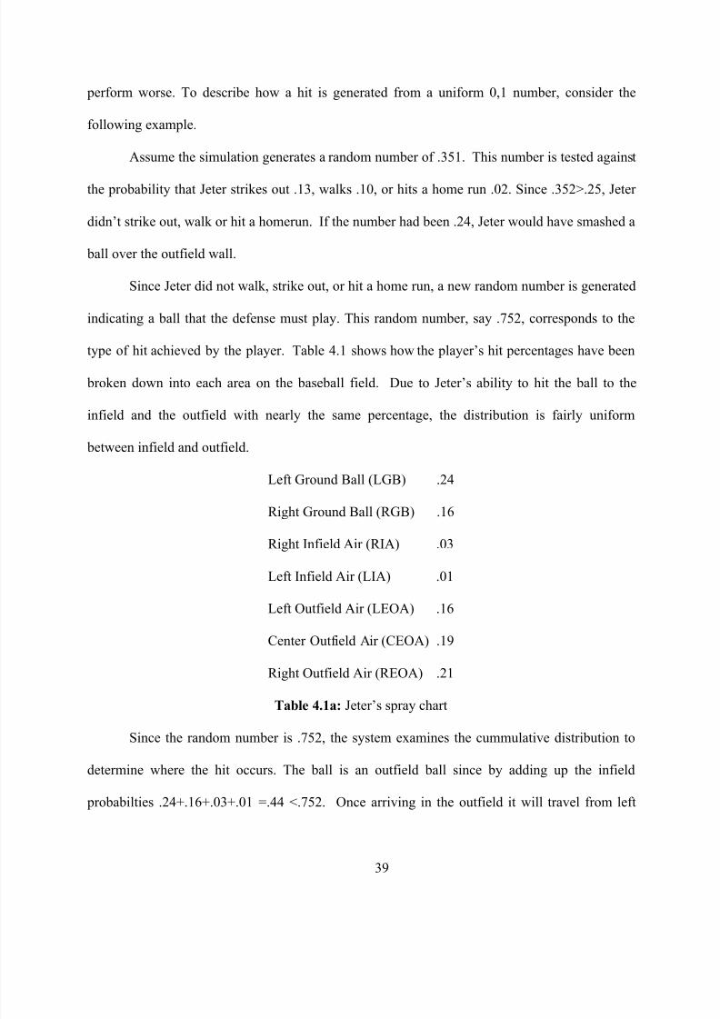
type of hit achieved by the player. Table 4.1 shows how the player’s hit percentages have been
broken down into each area on the baseball field. Due to Jeter’s ability to hit the ball to the
infield and the outfield with nearly the same percentage, the distribution is fairly uniform
between infield and outfield.
Left Ground Ball (LGB) .24
Right Ground Ball (RGB) .16
Right Infield Air (RIA) .03
Left Infield Air (LIA) .01
Left Outfield Air (LEOA) .16
Center Outfield Air (CEOA) .19
Right Outfield Air (REOA) .21
Table 4.1a: Jeter’s spray chart
Since the random number is .752, the system examines the cummulative distribution to
determine where the hit occurs. The ball is an outfield ball since by adding up the infield
probabilties .24+.16+.03+.01 =.44 <.752. Once arriving in the outfield it will travel from left

8/12/2019 Kyle Becker2009
http://slidepdf.com/reader/full/kyle-becker2009 49/73
40
field into center since the left field probability brings this probalility to .16+.44=.60. The hit was
not to right field since .60+.19=.79 > .752. Therefore the hit must be corresponding to
centerfield.
Now that the ball is known to be hit someplace in centerfield, the location and type of hit
must be determined. These calculations assume a uniformity in player depth. First, for each i
row, the probability increases by .02375 = .19/(11-4+1) uniformly over the space. Therefore the
hit is being played on the sixth row up in centerfield, or i=10. This is found by dividing the
remaining probability by the amount of incease per row; .152/.02375=6.4. Notice that this is
then the seventh largest depth in the outfield, because any number between 0 and 1 would be
assigned i=4.
The j location can be found similarly. There are 19 width locations in the outfield and 6
are assigned to left and rightfield and 7 are assigned to centerfield. So the probability of any
given width is 1/7 = .1428. To determine the j location divide the remainder by 1/7, which is
.4/(1/7) = 2.8. Therefore, the j location is the third width in the centerfield or j=9.
Finally, a speed must be determined. Since there are 6 speeds, the probability of any
speed is 1/6. Thus, the speed in this case follows a similar logic to the other cases and is derived
by taking .8/(1/6) = 4.8. Thus, the speed is assigned to speed 5.
Therefore, the random number .752 results in a ball that is hit to the location i=10 j=9,
and speed = 5. Thus, this hit went to the right of straight away center close to the warning track.
It is most likely a lazy pop fly and results in an out. However, if the center fielder was playing
the left field gap, then Jeter or any player would have a triple. In conclusion, the location for
each hit gerenated is a tedious procedure for an individual, but easy for a computer.

8/12/2019 Kyle Becker2009
http://slidepdf.com/reader/full/kyle-becker2009 50/73
41
4.1.3 H its and Outcomes
In order for this simulation to act like a true defense, the defense needs to think like a
baseball team. For this to happen, a “distance” measurement was created so that the defense
could choose the correct player to play the ball every time. Also this “distance” measurement
forces only one player to play the ball. The player’s “distance” is calculated by determining the
distance from the player’s starting position to where the ball is being played.
The formula for this distance is found by subtracting the player’s i and j distances from
hit’s i and j locations. However, if the player’s depth is less than the hit’s depth, or the bal l has
been hit over a player’s head; then he is penalized and the distance to the hit’s i location is
doubled. The distances are then compared for each hit, and the player with the least amount of
distance plays the ball. Shown in figure 4.1.3 is the formula that is used by the simulation to
accurately field a ball hit to a player:
dist=(i player -ihit )2+( j player -jhit )
2 for all ihit≤i player
dist=(i player -2*ihit )2+( j player -*jhit )
2 for all ihit>i player
Figure 4.1.3: Distance Calculation
The hits and outcomes decision area within the model was one of the most crucial, and
difficult to model. This area contained about 1,000 lines of code. This code described the
different scenarios that a defense would play against a batter. These scenarios labeled each hit
with a multiple different titles. The true actions of this code are better explained through a
couple of examples shown below:
A ball is hit at the coordinates 6,3 with a speed of 2. If a rightfielder is playing at the i,j
coordinates 7,4, with a speed of 5, and an error rate of .025 and the centerfielder is playing at the
coordinates 8,10 with a speed of 5 and error rate of .025.; the following hits may occur with

8/12/2019 Kyle Becker2009
http://slidepdf.com/reader/full/kyle-becker2009 51/73
42
some probability. This scenario is shown in figure 4.1.4 with the player locations and the ball
location.
Figure 4.1.4: Example 1 hit
First, the simulation will decide which player will play the ball. Shown in figure 4.1.5 is
the distance calculation for this hit. Equation (1) shows the calculation for the rightfielder’s
distance; while equation (2) shows the centerfielder’s distance. It is trivially shown that the
rightfielder will play the ball.
(7-6)2+(4-3)
2=2 (1)
(8-6)2+(10-3)
2=53 (2)
Figure 4.1.5: Distance Calculation
After determining which outfielder plays the ball, it is now important to decide whether
the hit is an error or not. In this case, the fielder is close to where the ball lands and should make

8/12/2019 Kyle Becker2009
http://slidepdf.com/reader/full/kyle-becker2009 52/73
43
the out or be charged with an error. A random number is generated using the rand() function
again and divided by the maximum number within C . This is then compared to the defensive
player’s error rate. If the random number is less than the error rate then the hit will result in an
error; for a rightfield error the hit type is ROAERROR, where ROA stands for right outfield air.
If the random number is greater than the error rate, then the ball is played by the defense
according to a series of rules.
If the rightfielder can make an out on the play then the resulting hit type will be
ROAOUT, if not then the resultant hit type could be a ROASINGLE, ROADOUBLE or
ROATRIPLE. If the rightfielder is playing in the right-center gap then the ball rolls all the way
to the wall; resulting in an ROATRIPLE. If the rightfielder starts deep, near the warning track,
then the player would play the ball in front of him and hold the runner to a single, ROASINGLE.
Another example would be using a ball hit in the infield near the hole by the shortstop
and third baseman. The ball has a hit location of 2,16 , with a speed of 2. This ball is hit
relatively slow and in the hole. The fielders are located at 2,18, and 3, 14. This scenario is
shown in figure 4.1.6, and the distance calculation is made in figure 4.1.7.

8/12/2019 Kyle Becker2009
http://slidepdf.com/reader/full/kyle-becker2009 53/73
44
(2-2)2+(17-16)
2=1 (1)
(3-2)
2
+(14-16)
2
=5 (2)
Figure 4.1.6: Example 2 hit Figure 4.1.7: Distance Calculation
By once again performing the distance calculation the lowest distance was 1. This
corresponds to the calculation shown in figure 4.1.7, equation (1). This distance is for the third
baseman to make the play. Once he has been chosen it is time to decide if he makes an error. If
his error rate is .025, and the error calculation relays .005; then the output would be an error on
the third baseman, or left infield error (LIERROR).
If the third baseman is playing in line with the ball than it becomes a routine play that he
makes easily. However, if he is playing close to the line and up on the grass, than there is no
way that he can make the play and throw the runner out at first, causing the hit to be a single.
With the placement of the ball, there is no way that it can be anything more than a single; that is
unless Manny Ramirez is playing left field.

8/12/2019 Kyle Becker2009
http://slidepdf.com/reader/full/kyle-becker2009 54/73
45
4.1.4 MOVEMENT OF RUNNERS
The movement of runners in baseball is a key aspect of the game. Rarely do the base
runners simply go base to base, and the simulation must reflect this unique feature of the game.
Depending upon a hit, a base runner may take multiple bases. To effectively implement these
ideas an intense case by case analysis is created. Approximately 1,000 lines of code enabled for a
fairly exhaustive set of situations to be analyzed. How this code functions is best described by
the next two examples.
Assume there is a base runner on first base, and there is a ball hit into right field, and the
outcome is a ROASINGLE. This ball will directly result in the runner on first advancing to third
base due to this throw being a long throw. However if this hit type had either been a
LOASINGLE, leftfield air single, or COASINGLE, centerfield air single, then the runner will
stop at second base since these throws to third are considerably shorter.
Another determining factor on the movement of runners is the number of outs in an
inning. If there is a runner on second with one out and a pop fly is hit, semi-shallow in the
outfield so that they are unable to tag up; then this runner will stay at the base. However if there
are two outs and the same scenario occurs, then it is likely that the runner will score easily since
he will be running once contact is made. This advancement of runners is accounted for in each
simulation model.

8/12/2019 Kyle Becker2009
http://slidepdf.com/reader/full/kyle-becker2009 55/73
46
4.2 Veracity of Model
It can be shown through statistics that the numbers produced through this simulation are
very accurate. Shown in table 4.2 are Derek Jeter’s season and lifetime batting averages and
slugging percentages.
Slg BA
0.430 0.314
0.405 0.291
0.481 0.324
0.552 0.349
0.481 0.339
0.480 0.311
0.421 0.2970.450 0.324
0.471 0.292
0.450 0.309
0.483 0.343
0.452 0.322
0.408 0.300
0.465 0.334
Lifetime 0.459 0.318
Table 4.2: Derek Jeter’s Statistics
The validity of the model is tested against these statistics. The comparison method
chosen is the paired t -test. This test includes a test of the p-value, which will test whether the
means are equal. It also includes a 95% confidence interval, if there is not a statistical difference
in the means, then this interval will include zero. The testing was conducted in Minitab 15.
4.2.1 Batting Average Test
Derek Jeter’s lifetime batting average is .317, as shown in table 4.2. This is an average
over 14 seasons; while the simulation was run for 50 seasons to comply with the Central Limit

8/12/2019 Kyle Becker2009
http://slidepdf.com/reader/full/kyle-becker2009 56/73
47
Theorem approximation. Shown in figure 4.2.1 are the results from the t -test performed between
the 50 simulated seasons with a base defense and the real statistics of Derek Jeter.
Two-Sample T-Test and CI: REAL BA, BASEBA
Two-sample T for REAL BA vs BASEBA
N Mean StDev SE Mean
REAL BA 14 0.3178 0.0190 0.0051
BASEBA 50 0.3088 0.0215 0.0030
Difference = mu (REAL BA) - mu (BASEBA)
Estimate for difference: 0.00895
95% CI for difference: (-0.00329, 0.02118)
T-Test of difference = 0 (vs not =): T-Value = 1.51 P-Value = 0.144 DF = 23
Figure 4.2.1: Batting Average t -test
The first area of comparison is the average values for Jeter’s batting average within the
two samples. His lifetime batting average is .317, which is nine points higher than his average
through the simulation. However, this difference is minimal since the players and stadiums that
he is playing against are held static. The standard errors of the means are also extremely close,
this allows the initial assumption of the means being equal to be drawn.
One of the strongest areas of comparison is a creation of a confidence interval of the
means. The t -test created a 95% confidence interval, and again if the confidence interval
includes zero then we may conclude that we fail to reject the null hypothesis that the means are
the same.
The final area of testing that was considered was the p-value. If the p-value is above .05
then once again we fail to reject the hypothesis that the means are different. For this t -test the p-
value was .144, which corresponds to the failure to reject the hypothesis.
4.2.2 Slugging Percentage Test
The comparison methods and testing are the same for testing the slugging percentage.
Again we tested the means to ensure through a t -test they were not different. Derek Jeter’s
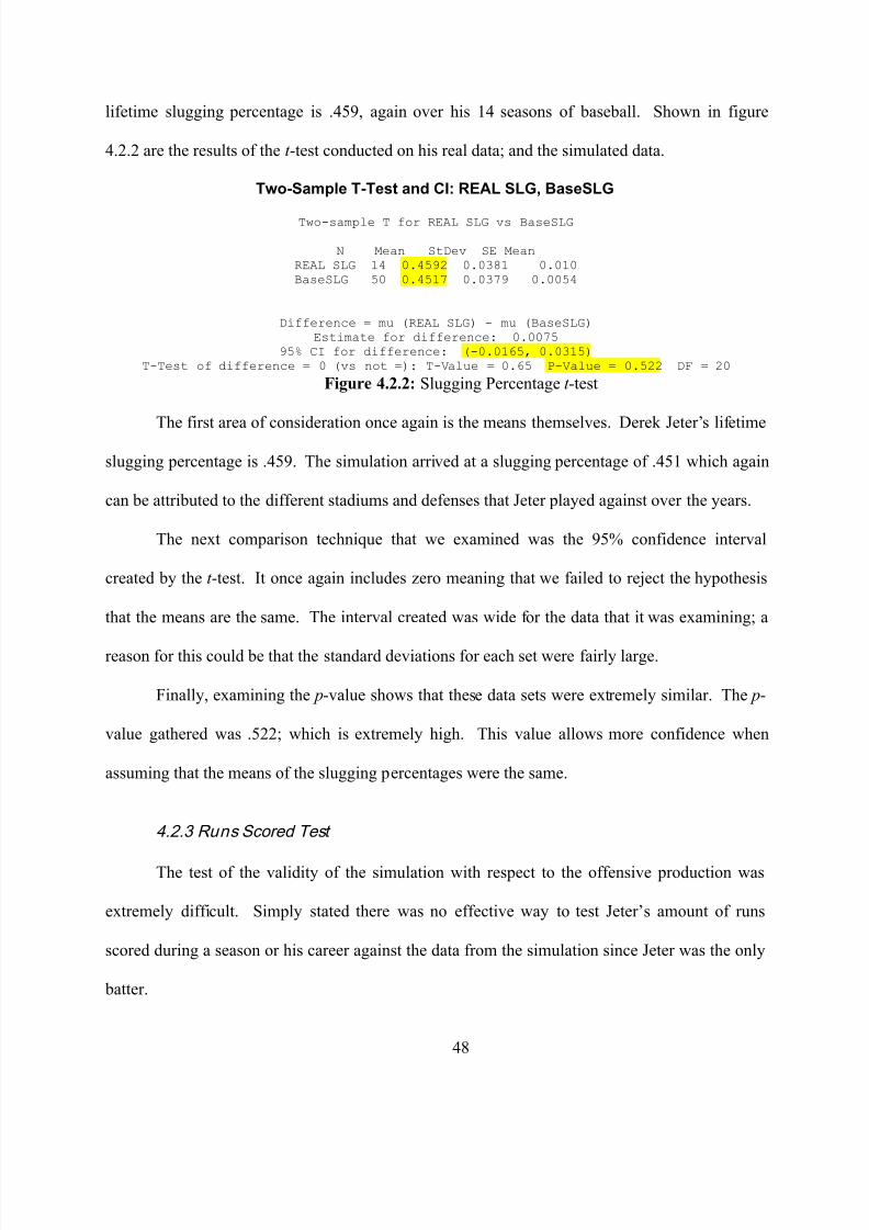
8/12/2019 Kyle Becker2009
http://slidepdf.com/reader/full/kyle-becker2009 57/73
48
lifetime slugging percentage is .459, again over his 14 seasons of baseball. Shown in figure
4.2.2 are the results of the t -test conducted on his real data; and the simulated data.
Two-Sample T-Test and CI: REAL SLG, BaseSLG
Two-sample T for REAL SLG vs BaseSLG
N Mean StDev SE Mean
REAL SLG 14 0.4592 0.0381 0.010
BaseSLG 50 0.4517 0.0379 0.0054
Difference = mu (REAL SLG) - mu (BaseSLG)
Estimate for difference: 0.0075
95% CI for difference: (-0.0165, 0.0315)
T-Test of difference = 0 (vs not =): T-Value = 0.65 P-Value = 0.522 DF = 20
Figure 4.2.2: Slugging Percentage t -test
The first area of consideration once again is the means themselves. Derek Jeter’s lifetime
slugging percentage is .459. The simulation arrived at a slugging percentage of .451 which again
can be attributed to the different stadiums and defenses that Jeter played against over the years.
The next comparison technique that we examined was the 95% confidence interval
created by the t -test. It once again includes zero meaning that we failed to reject the hypothesis
that the means are the same. The interval created was wide for the data that it was examining; a
reason for this could be that the standard deviations for each set were fairly large.
Finally, examining the p-value shows that these data sets were extremely similar. The p-
value gathered was .522; which is extremely high. This value allows more confidence when
assuming that the means of the slugging percentages were the same.
4.2.3 Runs Scored Test
The test of the validity of the simulation with respect to the offensive production was
extremely difficult. Simply stated there was no effective way to test Jeter’s amount of runs
scored during a season or his career against the data from the simulation since Jeter was the only
batter.

8/12/2019 Kyle Becker2009
http://slidepdf.com/reader/full/kyle-becker2009 58/73
49
With that being said it is fair to conclude that his run production is accurate due to his
batting average and slugging percentage being represented accurately. Both of these statistics
are correlated to the number of runs a team produces. Thus we can assume that the modeled
simulation is correct when approximating Derek Jeter’s career batting statistics.
4.3 Optimizing Defensive Alignments
The results for each piece of the simulation were incredibly positive. The test for the
different simulations was whether the defenses generated by OPL studio were statistically
different than the base defense shown in sections 4.2.1 and 4.2.2. These two sections explain
why these the base defense may be used as real life and may provide better outcomes. Shown in
figure 4.3 are the different alignments that are being tested.
Base Defense “Doubles Prevent”
BAIP alignment SPIP alignmentFigure 4.3: Baseball Alignments

8/12/2019 Kyle Becker2009
http://slidepdf.com/reader/full/kyle-becker2009 59/73
50
4.3.1 Batting Average Models
The first model created by OPL studio was generated by an IP named BAIP. This IP
aimed to generate a defense that would produce a defense that would reduce a player’s batting
average. For the test it was given Derek Jeter’s batting statistics from 2009. Shown in table
4.3.1 is a comparison of the batting averages generated using the base defense, a “Doubles
Prevent” defense, and the two OPL studio defenses.
BASEBA DeepBA BAIPBA SPIPBA
0.283 0.300 0.276 0.281
0.281 0.298 0.250 0.274
0.294 0.344 0.269 0.291
0.319 0.302 0.297 0.311
0.280 0.305 0.242 0.243
0.305 0.310 0.253 0.283
0.290 0.337 0.312 0.273
0.322 0.341 0.285 0.310
0.363 0.324 0.320 0.322
0.317 0.334 0.285 0.277
0.293 0.337 0.334 0.295
0.289 0.296 0.274 0.289
0.330 0.308 0.296 0.271
0.290 0.340 0.237 0.250
0.303 0.298 0.317 0.309
0.316 0.326 0.267 0.290
0.290 0.331 0.287 0.281
0.296 0.300 0.273 0.288
0.327 0.319 0.305 0.303
0.348 0.340 0.321 0.331
0.309 0.340 0.299 0.289
0.334 0.334 0.340 0.353
0.323 0.349 0.296 0.280
0.285 0.290 0.263 0.2960.311 0.295 0.331 0.286
0.318 0.318 0.277 0.266
0.325 0.341 0.291 0.299
0.271 0.305 0.280 0.292
0.292 0.297 0.285 0.284
0.312 0.320 0.291 0.298

8/12/2019 Kyle Becker2009
http://slidepdf.com/reader/full/kyle-becker2009 60/73
51
0.301 0.334 0.285 0.291
0.317 0.314 0.262 0.272
0.304 0.323 0.285 0.257
0.325 0.341 0.307 0.318
0.357 0.330 0.333 0.344
0.328 0.373 0.319 0.302
0.314 0.323 0.305 0.285
0.314 0.303 0.306 0.289
0.279 0.274 0.268 0.279
0.296 0.286 0.278 0.261
0.343 0.328 0.324 0.302
0.317 0.314 0.267 0.288
0.332 0.327 0.292 0.262
0.325 0.341 0.264 0.265
0.326 0.308 0.304 0.315
0.309 0.336 0.290 0.2970.291 0.323 0.302 0.312
0.277 0.300 0.251 0.258
0.286 0.277 0.277 0.292
0.283 0.284 0.299 0.288
Average 0.309 0.318 0.289 0.290
Table 4.3.1: BA Comparison
All four defensive strategies had fairly similar numbers. In order to compare the defenses
against the base defense, we once again used Minitab 15. The test of choice was the t -test and
the results from the first t -test; a test of the batting averages produced between the base defense
and the “Doubles Prevent” defense is shown in figure 4.3.1a. The r est of the t -tests follow this
initial test.
Two-Sample T-Test and CI: BASEBA, DeepBA
Two-sample T for BASEBA vs DeepBA
N Mean StDev SE Mean
BASEBA 50 0.3088 0.0215 0.0030
DeepBA 50 0.3183 0.0211 0.0030
Difference = mu (BASEBA) - mu (DeepBA)
Estimate for difference: -0.00950
95% CI for difference: (-0.01794, -0.00105)
T-Test of difference = 0 (vs not =): T-Value = -2.23 P-Value = 0.028 DF = 97
Figure 4.3.1a: Base vs. Deep t -test

8/12/2019 Kyle Becker2009
http://slidepdf.com/reader/full/kyle-becker2009 61/73
52
The results from this test reveal that in fact the batting average is not the same from the
base defense to the late innings “Doubles Prevent” defense. Even more, this defense will
increase a batter’s batting average, by examining the means, the batting average was raised by 10
points. With the confidence interval not including zero, we reject the hypothesis of the means
being equal. This theory is completely supported by the p-value being less than .05 at a value of
.028. Thus the standard defense will hold a player’s batting average lower.
Two-Sample T-Test and CI: BASEBA, BAIPBA
Two-sample T for BASEBA vs BAIPBA
N Mean StDev SE Mean
BASEBA 50 0.3088 0.0215 0.0030
BAIPBA 50 0.2893 0.0247 0.0035
Difference = mu (BASEBA) - mu (BAIPBA)
Estimate for difference: 0.01949
95% CI for difference: (0.01030, 0.02868)
T-Test of difference = 0 (vs not =): T-Value = 4.21 P-Value = 0.000 DF = 96
Figure 4.3.1b: Base vs BAIP batting averageThis t -test revealed that the OPL studio defense generated to lower a player’s batting
average is in fact different than a normal defense. This defense has a mean batting average about
20 points lower than the base defense. This t -test revealed that the confidence interval again
does not include zero and so we reject the hypothesis of the means being equal. The p-value
supports this claim with it being less than .05 at .000. This defense completely fulfilled its
objective of lowering a player’s batting average.
Two-Sample T-Test and CI: BASEBA, SPIPBA
Two-sample T for BASEBA vs SPIPBA
N Mean StDev SE Mean
BASEBA 50 0.3088 0.0215 0.0030
SPIPBA 50 0.2898 0.0222 0.0031
Difference = mu (BASEBA) - mu (SPIPBA)
Estimate for difference: 0.01908
95% CI for difference: (0.01041, 0.02775)
T-Test of difference = 0 (vs not =): T-Value = 4.37 P-Value = 0.000 DF = 97
Figure 4.3.1c: BASE vs SPIP batting average

8/12/2019 Kyle Becker2009
http://slidepdf.com/reader/full/kyle-becker2009 62/73
53
The t -test in this case proved that the SPIP provides a statistically better defense in
regards to batting average. The means are different by about 20 points and the confidence
interval does not include zero.
4.3.2 Slugging Percentage Models
The slugging percentage models are tested in the same fashion as the batting average
models. Since the base defense produced such a statistically similar slugging percentage then we
can use this as the real defense that plays against Jeter. Shown in table 4.3.2 are the collective
slugging percentages for each of the defense when run in a simulation.
BaseSLG DeepSLG BAIPSLG SPIPSLG
0.402 0.398 0.452 0.414
0.400 0.362 0.460 0.364
0.422 0.451 0.459 0.401
0.473 0.403 0.499 0.454
0.416 0.420 0.412 0.378
0.405 0.378 0.445 0.372
0.436 0.437 0.473 0.494
0.471 0.463 0.549 0.448
0.549 0.448 0.523 0.4880.448 0.413 0.458 0.446
0.463 0.501 0.520 0.521
0.450 0.406 0.486 0.435
0.500 0.391 0.442 0.482
0.426 0.443 0.387 0.363
0.454 0.405 0.507 0.491
0.432 0.438 0.449 0.385
0.400 0.410 0.451 0.423
0.450 0.398 0.506 0.452
0.495 0.439 0.473 0.474
0.509 0.441 0.503 0.464
0.439 0.418 0.444 0.454
0.499 0.459 0.589 0.548
0.496 0.470 0.438 0.440
0.392 0.356 0.491 0.415
0.450 0.395 0.456 0.501
0.484 0.411 0.460 0.444

8/12/2019 Kyle Becker2009
http://slidepdf.com/reader/full/kyle-becker2009 63/73
54
0.499 0.489 0.491 0.456
0.394 0.384 0.475 0.432
0.384 0.328 0.418 0.414
0.460 0.400 0.447 0.450
0.439 0.441 0.464 0.428
0.435 0.378 0.406 0.394
0.480 0.447 0.468 0.476
0.482 0.453 0.500 0.446
0.495 0.406 0.539 0.527
0.487 0.507 0.505 0.463
0.439 0.409 0.454 0.477
0.481 0.401 0.471 0.490
0.408 0.366 0.430 0.410
0.418 0.360 0.423 0.414
0.490 0.423 0.495 0.506
0.508 0.464 0.471 0.4320.443 0.410 0.412 0.425
0.453 0.440 0.427 0.396
0.488 0.420 0.496 0.461
0.464 0.418 0.501 0.454
0.400 0.425 0.503 0.479
0.430 0.418 0.448 0.408
0.426 0.404 0.471 0.401
0.423 0.353 0.510 0.494
Average 0.452 0.418 0.471 0.446
Table 4.3.2: SP Comparison
The slugging percentages shown in the table look fairly similar. In order to get a better
feel for which defenses reduce a batter’s slugging percentage the best, a t -test of the data was
performed once again. The results of this test are shown throughout the rest of the section.
Two-Sample T-Test and CI: BaseSLG, DeepSLG
Two-sample T for BaseSLG vs DeepSLG
N Mean StDev SE MeanBaseSLG 50 0.4517 0.0379 0.0054
DeepSLG 50 0.4180 0.0376 0.0053
Difference = mu (BaseSLG) - mu (DeepSLG)
Estimate for difference: 0.03372
95% CI for difference: (0.01872, 0.04872)
T-Test of difference = 0 (vs not =): T-Value = 4.46 P-Value = 0.000 DF = 97
Figure 4.3.2a: Base vs. Deep Slugging Percentage
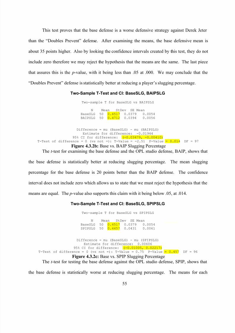
8/12/2019 Kyle Becker2009
http://slidepdf.com/reader/full/kyle-becker2009 64/73
55
This test proves that the base defense is a worse defensive strategy against Derek Jeter
than the “Doubles Prevent” defense. After examining the means, the base defensive mean is
about 35 points higher. Also by looking the confidence intervals created by this test, they do not
include zero therefore we may reject the hypothesis that the means are the same. The last piece
that assures this is the p-value, with it being less than .05 at .000. We may conclude that the
“Doubles Prevent” defense is statistically better at reducing a player’s slugging percentage.
Two-Sample T-Test and CI: BaseSLG, BAIPSLG
Two-sample T for BaseSLG vs BAIPSLG
N Mean StDev SE Mean
BaseSLG 50 0.4517 0.0379 0.0054
BAIPSLG 50 0.4712 0.0394 0.0056
Difference = mu (BaseSLG) - mu (BAIPSLG)
Estimate for difference: -0.01944
95% CI for difference: (-0.03479, -0.00410)
T-Test of difference = 0 (vs not =): T-Value = -2.51 P-Value = 0.014 DF = 97
Figure 4.3.2b: Base vs. BAIP Slugging PercentageThe t -test for examining the base defense and the OPL studio defense, BAIP, shows that
the base defense is statistically better at reducing slugging percentage. The mean slugging
percentage for the base defense is 20 points better than the BAIP defense. The confidence
interval does not include zero which allows us to state that we must reject the hypothesis that the
means are equal. The p-value also supports this claim with it being below .05, at .014.
Two-Sample T-Test and CI: BaseSLG, SPIPSLG
Two-sample T for BaseSLG vs SPIPSLG
N Mean StDev SE Mean
BaseSLG 50 0.4517 0.0379 0.0054
SPIPSLG 50 0.4457 0.0431 0.0061
Difference = mu (BaseSLG) - mu (SPIPSLG)
Estimate for difference: 0.00606
95% CI for difference: (-0.01005, 0.02217)
T-Test of difference = 0 (vs not =): T-Value = 0.75 P-Value = 0.457 DF = 96
Figure 4.3.2c: Base vs. SPIP Slugging PercentageThe t -test for testing the base defense against the OPL studio defense, SPIP, shows that
the base defense is statistically worse at reducing slugging percentage. The means for each

8/12/2019 Kyle Becker2009
http://slidepdf.com/reader/full/kyle-becker2009 65/73
56
defense are around 6 points apart. The confidence intervals include zero which allows us to state
that we fail to reject the hypothesis that the means are equal. The p-value also supports this
claim with it being above .05, at .457. Thus there is insignificant evidence to rule which defense
is better with respect to slugging percentage.
4.3.3 Run Reducti on Test
The final piece of a good defense is its ability to limit run production. The simulation
results for all four defenses in terms of run reduction are shown in table 4.3.3. The defenses
were judged on their ability to limit runs per game. Also special consideration was taken when
judging a defense’s ability to keep a large run total down.
BaseRUN DeepRUN BAIPRUN SPIPRUN
3 2 4 6
1 3 1 3
4 8 4 5
4 9 5 8
1 1 7 5
4 4 2 5
1 0 1 5
4 4 5 8
2 4 2 4
6 4 4 5
1 1 2 1
4 1 3 4
3 3 3 1
2 0 1 3
0 0 1 8
2 2 3 2
2 2 4 5
2 0 4 2
3 3 5 4
1 1 2 2
1 2 2 4
1 3 3 3
3 3 4 9
3 8 7 9

8/12/2019 Kyle Becker2009
http://slidepdf.com/reader/full/kyle-becker2009 66/73
57
Average Runs
Maximum Runs
4 5 4 17
8 3 13 2
1 1 0 5
4 4 5 4
2 5 3 8
3 2 1 7
2 9 2 4
10 6 7 7
2 4 5 9
3 6 4 2
1 3 1 1
6 0 2 3
2 0 0 3
0 5 0 2
7 2 5 7
4 5 3 61 0 3 1
0 7 2 5
3 3 5 6
4 6 3 13
19 8 15 10
4 3 4 1
7 1 8 1
0 0 0 4
7 1 2 1
3.306122 3.204082 3.591837 4.897959
19 9 15 17
Table 4.3.3: Run Reduction AnalysisAfter examining both the runs allowed per game and the maximum runs allowed it
appears that the “Doubles Prevent” defense does the best job of limiting offense. It was able to
reduce the runs much better than any of the other defenses. The two OPL defenses struggled
reducing the amount of runs given up, which is surprising since they were able to reduce both the
batting average and the slugging percentage. The discussion of a run reduction IP is in section
5.1.1.

8/12/2019 Kyle Becker2009
http://slidepdf.com/reader/full/kyle-becker2009 67/73
58
Chapter 5 Continuing Research
Baseball is a very lucrative game, and with the popularity increasing, it should continue
to be in the future. This thesis laid the ground work for a very interesting and productive area of
research in this field. The models and IP’s associated with this thesis show how complex
baseball is. However, more importantly they show that baseball may be modeled, and modeled
effectively at that.
This thesis proved that the best defense to play is not one that is currently being used, but
one that was created by an IP. This defense reduced a batter’s batting average. If a team desires
to reduce a player’s slugging percentage, then they should also use a non-traditional defense.
5.1 Future Research
The models mentioned in this work are just starting blocks for future research. The first
area that can be expanded on is the use of the pitcher, not only for defense, but in terms of pitch
selection and fatigue. Currently MLB.com not only has hit charts available, but there is an equal
amount of information relating to the pitchers; including how fatigue affects their ability to
locate a pitch.
By integrating a pitcher into the simulation a user will actually see how a manager can
impact a game. A pitcher could start out the game with a variable representing them, and as the
game wore on; or as they became tired or the offense was hitting better this variable would
decrease, similar to real life. Once this variable dropped below a preset value, then a manager
could actually call to the bullpen to bring in a reliever.
With respect to offense, an IP and a simulation must not only be able to create and test a
defense for one player, but for an entire team. The IP portion of this would be similar to the

8/12/2019 Kyle Becker2009
http://slidepdf.com/reader/full/kyle-becker2009 68/73

8/12/2019 Kyle Becker2009
http://slidepdf.com/reader/full/kyle-becker2009 69/73
60
In actuality this could be tailored to a specific situation. For instance, in the early innings
of a National League game, a single with two outs by the 8 th batter would have a small penalty
because he is unlikely to score since the pitcher is up next. In contrast, having the third batter in
the lineup get a single in this situation greatly increases the probability of a run being scored.
By creating the benefit matrices for each situation, the IP will be able to adapt its
defensive setup to the situation, which should dramatically reduce the number of runs allowed by
a team. Forward thinking teams should take advantage of this research and be the first to jump
on this bandwagon before it becomes a common practice.

8/12/2019 Kyle Becker2009
http://slidepdf.com/reader/full/kyle-becker2009 70/73
61
References
AP ONLINE (2001). “A’s OK Jason Giambi’s No-Trade Clause”.
http://www.highbeam.com/doc/1P1-47714259.html. 2009.
Baseballcube.com (2009). Nomar Garciaparra’s Career Statistics and Contracts.
http://www.thebaseballcube.com/Salaries/G/Nomar-Garciaparra.shtml. 2009.
Brittain, B. (1992). All the Money in the World, HarperCollins Publishers.
Becker, A. D. (1994). The Sherman Antitrust Act,
http://www.stolaf.edu/people/becker/antitrust/statutes/sherman.html.2009.
Begel, A., Blelloch, G. (1998). Algorithms in the Real World. Lecture #10 Linear Programming.
http://74.125.47.132/search?q=cache:_y_WOjMArcJ:www.cs.cmu.edu/afs/cs/project/psci
co-guyb/294/classtes/all/10.ps+history+integer+programming&cd=1&hl=
en&ct=clnk&gl=us. (2009).
Cheng, E., Steffy D. E. (2007). Clinching and Elimination of Playoff Berth in the
NHL.International Journal of Operations Research Vol. 5, No. 3, 187-192 (2008)
Crisco, J.J., Greenwald, R.M., Blume, J.D. , Penna, L.H. (2002). "Batting Performance of
Wood and Metal Baseball Bats," Med. Sci. Sports Exerc., 34(10), 1675-1684 (2002)
8/12/2019 Kyle Becker2009
http://slidepdf.com/reader/full/kyle-becker2009 71/73
62
Easton, K., Nemhauser, G., Trick, M. (2001) The Traveling Tournament Problem: Description
and Benchmarks, in: Proceedings CP'01, Lecture Notes in Computer Science 2239,
Springer, 580-585.
Faith, C. (2007). Way of the Turtle. McGraw Hill Books. New York, NY.
Fox, Hill (2004). Generating the Knoxville economy.
Gagliardi, R. (2009). “Orange Back Out of Game with UW.” Wyoming Tribune Eagle.
Hanna, W. T. (1972). A Simulation of the Human Heart Function. Biophysical Journal , Volume
13, Issue 7, Pages 603-621.
Karp R.M. (1972). "Reducibility Among Combinatorial Problems". in R. E. Miller and J. W.
Thatcher (editors). Complexity of Computer Computations. New York: Plenum. pp. 85 –
103.
Kendall, G., Knust, S., Ribeiro, C.C., Urrutia, S. (2010) Scheduling in Sports: An Annotated
Bibliography, Computers and Operations Research 37, 1-19.
Klingstam, P., Olsson, B.G. (2000). Application of Simulation for Manufacturing Processes
Improvements: Using Simulation Techniques for Continuous Process Verification in
Industrial System Development. Winter Simulation Conference.

8/12/2019 Kyle Becker2009
http://slidepdf.com/reader/full/kyle-becker2009 72/73
63
MLB.com1 (2009). Official Baseball Rules. Mlb.com. 2009
MLB.com2 (2009). Winningest Managers of the previous decade. Mlb.com. 2009
MLB.com3 (2009). Texeira Signs Record Contract. Mlb.com. 2009
MLB.com4 (2009). Derek Jeter Hit Chart (2009). Mlb.com. 2009
Montalbano, E. (2008). “Computer Ranking System picks NCAA Tournament Final Four.”
IDG News Service. 2009.
Olsen, S. (2006). Blueprinting the Human Brain. http://news.cnet.com/Blueprinting-the-human-
brain/2100-11393_3-6071061.html. 2009.
Overton, M. L. (1997). Linear Programming. Draft for Encyclopedia Americana
December 20, 1997.
Parker, R. G. (1996). Deterministic Scheduling Theory. Taylor & Francis inc.
Payne, D. (1998). “Cell Simulator Brings Biochemistry to Life.” Chemistry and Industry.
December 21, 1998.

8/12/2019 Kyle Becker2009
http://slidepdf.com/reader/full/kyle-becker2009 73/73
Russell, D.A. (2003). “Why Aluminum Bats Perform Better Than Wood.”
http://paws.kettering.edu/~drussell/bats-new/alumwood.html. 2009.
Shenoy, G.V. (1998). Linear Programming: Methods and Applications. New AGF
International,1998.
Trick, M (2003). Integer and Constraint Programming Approaches for Round Robin
Tournament Scheduling. In E. Burke and P. De Causmaecker, editors, Practice and
Theory of AutomatedTimetabling IV , volume 2740 of Lecture Notes in Computer Science,
pages 63{77. Springer Berlin / Heidelberg.
Verbraeck, A., Valentin, E. (2002). Transportation Spplications of Simulation: Simulation
Building Blocks for Airport Terminal Modeling. Proceedings of the 34th conference on
Winter simulation: exploring new frontiers.
Vossen, T., Ball, M., Lotem, A., Nau, D. (1999). On the Use of Integer Programming Models in
AI Planning.
Wright, M.B. (2006). Scheduling Fixtures for Basketball New Zealand. Computers &
Operations Research, 33:1875{1893,