kirchhoff–love shell theory based on tangential

Computational Mechanics (2019) 64:113–131https://doi.org/10.1007/s00466-018-1659-5

ORIG INAL PAPER

Kirchhoff–Love shell theory based on tangential differential calculus

D. Schöllhammer1 · T. P. Fries1

Received: 28 May 2018 / Accepted: 14 November 2018 / Published online: 29 November 2018© The Author(s) 2018

AbstractThe Kirchhoff–Love shell theory is recasted in the frame of the tangential differential calculus (TDC) where differentialoperators on surfaces are formulated based on global, three-dimensional coordinates. As a consequence, there is no needfor a parametrization of the shell geometry implying curvilinear surface coordinates as used in the classical shell theory.Therefore, the proposed TDC-based formulation also applies to shell geometries which are zero-isosurfaces as in the level-setmethod where no parametrization is available in general. For the discretization, the TDC-based formulation may be usedbased on surface meshes implying element-wise parametrizations. Then, the results are equivalent to those obtained based onthe classical theory. However, it may also be used in recent finite element approaches as the TraceFEM and CutFEM whereshape functions are generated on a background mesh without any need for a parametrization. Numerical results presentedherein are achieved with isogeometric analysis for classical and new benchmark tests. Higher-order convergence rates in theresidual errors are achieved when the physical fields are sufficiently smooth.

Keywords Shells · Tangential differential calculus · TDC · Isogeometric analysis · IGA · Manifolds

1 Introduction

The mechanical modeling of shells leads to partial differen-tial equations (PDEs) on manifolds where the manifolds arecurved surfaces in the three-dimensional space. An overviewin classical shell theory is given, e.g., in [4,9,32,44,45]or in the textbooks [1,5,41,49]. When modeling physicalphenomena on curved surfaces, definitions for geometricquantities (normal vectors, curvatures, etc.) and differen-tial surface operators (gradients, divergence, etc.) are keyingredients. These quantities may be either defined based ontwo-dimensional, curvilinear local coordinates living on themanifold or on global coordinates of the surrounding, three-dimensional space.

In the first case, the curved surface is parametrizedby two parameters, i.e., there is a given map from thetwo-dimensional parameter space to the three-dimensional

B D. Schö[email protected]://www.ifb.tugraz.at

T. P. [email protected]://www.ifb.tugraz.at

1 Institute of Structural Analysis, Graz University ofTechnology, Lessingstr. 25/II, 8010 Graz, Austria

physical space, see Fig. 1a. For the definition of geometri-cal quantities and surface operators, co- and contra-variantbase vectors and Christoffel-symbols naturally occur. It isimportant to note that a parametrization of a surface is notunique, hence, there are infinitely many maps which result inthe same curved surface. Obviously, the physical modelingmust be independent of a concrete parametrization, whichsuggests the existence of a parametrization-free formulation.

In the second case, the geometric quantities and surfaceoperators are based on global coordinates as done in the tan-gential differential calculus (TDC) [15,25,28]. Then, amodelmay also be defined even if a parametrization of a curved sur-face does not exist, for example, when it is a zero-isosurfaceof a scalar function in three dimensions following the level-set method [21,22,39,43]. When the physical modeling isbased on the TDC, i.e., on global coordinates, it is applicableto surfaces which are parametrized or not. In this sense, theTDC-based approach is more general than approaches basedon local coordinates. Models based on the TDC are found invarious applications, see [16–18,22] for scalar problems suchas heat flow and [20,31] for flow problems on manifolds. Inthe context of structure mechanics, this approach is used in[29] for curved beams, in [25,26,28] for membranes, and in[27] for flat shells embedded in R3.

123

http://crossmark.crossref.org/dialog/?doi=10.1007/s00466-018-1659-5&domain=pdf

http://orcid.org/0000-0002-9285-5561

http://orcid.org/0000-0003-1210-1557

114 Computational Mechanics (2019) 64:113–131

(a) (b) (c) (d)

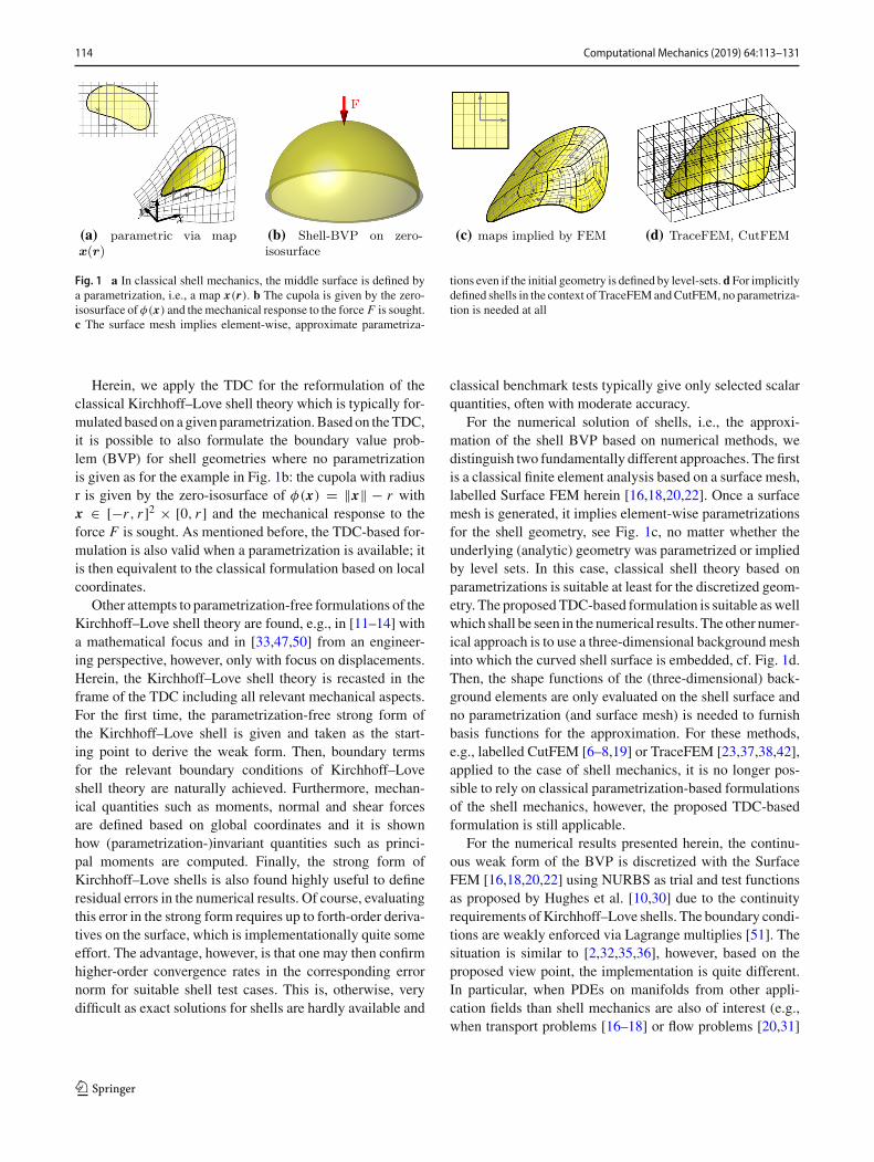
Fig. 1 a In classical shell mechanics, the middle surface is defined bya parametrization, i.e., a map x(r). b The cupola is given by the zero-isosurface of φ(x) and themechanical response to the force F is sought.c The surface mesh implies element-wise, approximate parametriza-

tions even if the initial geometry is defined by level-sets.d For implicitlydefined shells in the context of TraceFEMandCutFEM, no parametriza-tion is needed at all

Herein, we apply the TDC for the reformulation of theclassical Kirchhoff–Love shell theory which is typically for-mulated based on a given parametrization.Based on theTDC,it is possible to also formulate the boundary value prob-lem (BVP) for shell geometries where no parametrizationis given as for the example in Fig. 1b: the cupola with radiusr is given by the zero-isosurface of φ(x) = ‖x‖ − r withx ∈ [−r , r ]2 × [0, r ] and the mechanical response to theforce F is sought. As mentioned before, the TDC-based for-mulation is also valid when a parametrization is available; itis then equivalent to the classical formulation based on localcoordinates.

Other attempts to parametrization-free formulations of theKirchhoff–Love shell theory are found, e.g., in [11–14] witha mathematical focus and in [33,47,50] from an engineer-ing perspective, however, only with focus on displacements.Herein, the Kirchhoff–Love shell theory is recasted in theframe of the TDC including all relevant mechanical aspects.For the first time, the parametrization-free strong form ofthe Kirchhoff–Love shell is given and taken as the start-ing point to derive the weak form. Then, boundary termsfor the relevant boundary conditions of Kirchhoff–Loveshell theory are naturally achieved. Furthermore, mechan-ical quantities such as moments, normal and shear forcesare defined based on global coordinates and it is shownhow (parametrization-)invariant quantities such as princi-pal moments are computed. Finally, the strong form ofKirchhoff–Love shells is also found highly useful to defineresidual errors in the numerical results. Of course, evaluatingthis error in the strong form requires up to forth-order deriva-tives on the surface, which is implementationally quite someeffort. The advantage, however, is that one may then confirmhigher-order convergence rates in the corresponding errornorm for suitable shell test cases. This is, otherwise, verydifficult as exact solutions for shells are hardly available and

classical benchmark tests typically give only selected scalarquantities, often with moderate accuracy.

For the numerical solution of shells, i.e., the approxi-mation of the shell BVP based on numerical methods, wedistinguish two fundamentally different approaches. The firstis a classical finite element analysis based on a surface mesh,labelled Surface FEM herein [16,18,20,22]. Once a surfacemesh is generated, it implies element-wise parametrizationsfor the shell geometry, see Fig. 1c, no matter whether theunderlying (analytic) geometry was parametrized or impliedby level sets. In this case, classical shell theory based onparametrizations is suitable at least for the discretized geom-etry. The proposedTDC-based formulation is suitable aswellwhich shall be seen in the numerical results. The other numer-ical approach is to use a three-dimensional background meshinto which the curved shell surface is embedded, cf. Fig. 1d.Then, the shape functions of the (three-dimensional) back-ground elements are only evaluated on the shell surface andno parametrization (and surface mesh) is needed to furnishbasis functions for the approximation. For these methods,e.g., labelled CutFEM [6–8,19] or TraceFEM [23,37,38,42],applied to the case of shell mechanics, it is no longer pos-sible to rely on classical parametrization-based formulationsof the shell mechanics, however, the proposed TDC-basedformulation is still applicable.

For the numerical results presented herein, the continu-ous weak form of the BVP is discretized with the SurfaceFEM [16,18,20,22] using NURBS as trial and test functionsas proposed by Hughes et al. [10,30] due to the continuityrequirements ofKirchhoff–Love shells. The boundary condi-tions are weakly enforced via Lagrange multiplies [51]. Thesituation is similar to [2,32,35,36], however, based on theproposed view point, the implementation is quite different.In particular, when PDEs on manifolds from other appli-cation fields than shell mechanics are also of interest (e.g.,when transport problems [16–18] or flow problems [20,31]

123

Computational Mechanics (2019) 64:113–131 115

on curved surfaces are considered), there is a unified andelegant way to handle this by computing surface gradientsapplied to finite element shape functions which simplifiesthe situation considerably. In that sense one may shift sig-nificant parts of the implementation needed for shells to theunderlying finite element technology and recycle this in othersituations where PDEs on surfaces are considered.

We summarize the advantages of the TDC-based formula-tion of Kirchhoff–Love shells: (1) the definition of the BVPdoes not need a parametrization of the surface (though it canalso handle the classical situation where a parametrizationis given), (2) the TDC-based formulation is also suitablefor very recent finite element technologies such as Cut-FEM and TraceFEM (though the typical approach basedon the Surface FEM or IGA is also possible and demon-strated herein), (3) the implementation is advantagous infinite element (FE) codes where other PDEs on manifoldsare considered as well due to the split of FE technology andapplication. From a didactic point of view, it may also beadvantageous that troubles with curvilinear coordinates (co-and contra-variance, Christoffel-symbols) are avoided in theTDC-based approach where surface operators and geometricquantities are expressed in tensor notation.

The outline of the paper is as follows: In Sect. 2, impor-tant surface quantities are defined, and an introduction to thetangential differential calculus (TDC) is given. In Sect. 3,the classical linear Kirchhoff–Love shell equations understatic loading are recast in terms of the TDC. Stress resultantssuch asmembrane forces, bendingmoments, transverse shearforces and corner forces are defined. In Sect. 4, implemen-tational aspects are considered. The element stiffness matrixand the resulting system of linear equations are shown. Theimplementation of boundary conditions based on Lagrangemultipliers is outlined. Finally, in Sect. 5, numerical resultsare presented. The first example is a flat shell embedded inR3, where an analytical solution is available. The second and

third example are parts of popular benchmarks as proposedin [2]. In the last example, a more general geometry withoutanalytical solution or reference displacement is considered.The error is measured in the strong form of the equilibriumin order to verify the proposed approach and higher-orderconvergence rates are achieved.

2 Preliminaries

Shells are geometrical objects, where one dimension is sig-nificantly smaller compared to the other two dimensions. Inthis case, the shell can be reduced to a surfaceΓ embedded inthe physical spaceR3. In particular, the surface is a manifoldof codimension 1. Let the surface be possibly curved, suffi-ciently smooth, orientable, connected and bounded by ∂Γ .There are two alternatives for defining the shell geometry.

One is through a parametrization, i.e., a (bijective) mapping

x(r) : Ω → Γ (1)

from the parameter space Ω ⊂ R2 to the real domain Γ ⊂

R3. The other approach is based on the level-set method.

Then, a level-set function φ(x) : R3 → Rwith x ∈ Ω ⊂ R3

exists and the shell is implicitly given by

Γ = {x : φ(x) = 0 ∀ x ∈ Ω} . (2)

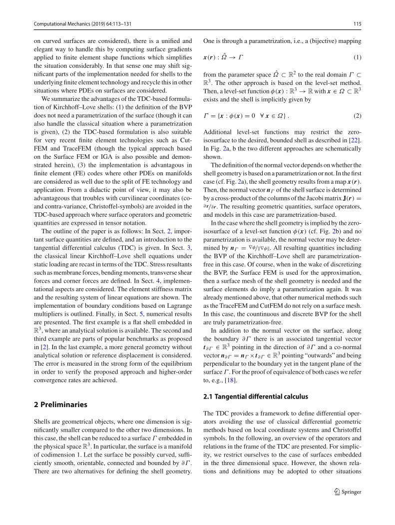
Additional level-set functions may restrict the zero-isosurface to the desired, bounded shell as described in [22].In Fig. 2a, b the two different approaches are schematicallyshown.

Thedefinitionof the normal vector depends onwhether theshell geometry is based on aparametrization or not. In thefirstcase (cf. Fig. 2a), the shell geometry results from amap x(r).Then, the normal vector nΓ of the shell surface is determinedby a cross-product of the columns of the Jacobimatrix J(r) =∂x/∂ r. The resulting geometric quantities, surface operators,and models in this case are parametrization-based.

In the casewhere the shell geometry is implied by the zero-isosurface of a level-set function φ(x) (cf. Fig. 2b) and noparametrization is available, the normal vector may be deter-mined by nΓ = ∇φ/‖∇φ‖. All resulting quantities includingthe BVP of the Kirchhoff–Love shell are parametrization-free in this case. Of course, when in the wake of discretizingthe BVP, the Surface FEM is used for the approximation,then a surface mesh of the shell geometry is needed and thesurface elements do imply a parametrization again. It wasalready mentioned above, that other numerical methods suchas the TraceFEM and CutFEM do not rely on a surface mesh.In this case, the countinuous and discrete BVP for the shellare truly parametrization-free.

In addition to the normal vector on the surface, alongthe boundary ∂Γ there is an associated tangential vectort∂Γ ∈ R

3 pointing in the direction of ∂Γ and a co-normalvector n∂Γ = nΓ × t∂Γ ∈ R

3 pointing “outwards” and beingperpendicular to the boundary yet in the tangent plane of thesurfaceΓ . For the proof of equivalence of both caseswe referto, e.g., [18].

2.1 Tangential differential calculus

The TDC provides a framework to define differential oper-ators avoiding the use of classical differential geometricmethods based on local coordinate systems and Christoffelsymbols. In the following, an overview of the operators andrelations in the frame of the TDC are presented. For simplic-ity, we restrict ourselves to the case of surfaces embeddedin the three dimensional space. However, the shown rela-tions and definitions may be adopted to other situations

123


Fig. 2 Examples of boundedsurfaces Γ embedded in thephysical space R3: a explicitlydefined surface with a map x(r),b implicitly defined surface witha master level-functionφ(x) = 0 (yellow) and slavelevel-set functions ψi for theboundary definition (gray)

(a) (b)

accordingly (e.g., curved lines embedded in 2D or 3D). Anintroduction from amoremathematical point of view is givenin [15,25,31].

Orthogonal projection operator P

The orthogonal projection operator or normal projector P ∈R3×3 is defined as

P = I − nΓ ⊗ nΓ . (3)

The operator ⊗ is the dyadic product of two vectors. Thenormal projector P projects a vector v onto the tangent spaceTPΓ of the surface. Note that P is idempotent (P · P = P),symmetric (P = Pᵀ) and obviously in the tangent space TPΓ

of the surface, i.e., P · nΓ = nᵀΓ · P = 0).

The projection of a vector field v : Γ → R3 onto the

tangent plane is defined by

vt = P · v ∈ TPΓ (4)

where vt is tangential, i.e. vt ·nΓ = 0. The double projectionof a second-order tensor function A(x) : Γ → R

3×3 leadsto an in-plane tensor and is defined as

At = P · A · P ∈ TPΓ , (5)

with the properties At = P·At ·P and At ·nΓ = nᵀΓ ·At = 0.

Tangential gradient of scalar functions

The tangential gradient ∇Γ of a scalar function u : Γ → R

on the manifold is defined as

∇Γ u(x) = P(x) · ∇u(x) , ∇Γ u(x) ∈ R3×1 , x ∈ Γ (6)

where ∇ is the standard gradient operator in the physicalspace and u is a smooth extension of u in a neighbourhoodU of the manifold Γ . Alternatively, u is given as a functionin global coordinates u(x) : R3 → R and only evaluated atthe manifold u|Γ = u.

For parametrized surfaces defined by the map x(r), and agiven scalar function u(r) : Ω → R, the tangential gradientcan be determinedwithout explicitly computing an extensionu using

∇Γ u(x(r)) = J(r) · G(r)−1 · ∇ru(r) , (7)

with J(r) = ∂x/∂ r ∈ R3×2 being the Jacobi matrix, G =

Jᵀ · J is the metric tensor or the first fundamental form andthe operator ∇r is the gradient with respect to the referencecoordinates. The components of the tangential gradient aredenoted by

∇Γ u =⎡⎣

∂Γx u

∂Γy u

∂Γz u

⎤⎦ , (8)

representing first-order partial tangential derivatives. Animportant property of ∇Γ u is that the tangential gradient ofa scalar-valued function is in the tangent space of the surface∇Γ u ∈ TPΓ , i.e., ∇Γ u · nΓ = 0. When using the SurfaceFEM to solve BVPs on surfaces, one may use Eq. (7) tocompute tangential gradients of the shape functions. If, onthe other hand, TraceFEM or CutFEM is used, one may useEq. (6).

Tangential gradient of vector-valued functions

Consider a vector-valued function v(x) : Γ → R3 and apply

to each component of v the tangential gradient for scalars.This leads to the directional gradient of v defined as

∇dirΓ v(x) = ∇dir

Γ

⎡⎣u(x)

v(x)

w(x)

⎤⎦ =

⎡⎣

∂Γx u ∂Γ

y u ∂Γz u

∂Γx v ∂Γ

y v ∂Γz v

∂Γx w ∂Γ

y w ∂Γz w

⎤⎦ . (9)

Note that the directional gradient is not in the tangent spaceof the surface, in general. A projection of the directionalgradient to the tangent space leads to the covariant gradient

123


of v and is defined as

∇covΓ v = P · ∇dir

Γ v , (10)

which is an in-plane tensor, i.e.,∇covΓ v ∈ TPΓ . The covariant

gradient often appears in the modelling of physical phenom-ena onmanifolds, i.e., in the governing equations. In contrastthe directional gradient appears naturally in product rules ordivergence theorems on manifolds.

In the following, partial surface derivatives of scalarfunctions are denoted as ∂Γ

xi u or uΓ,i with i = 1, 2, 3. Par-

tial surface derivatives of vector or tensor components aredenoted as vdiri, j for directional and vcovi, j for covariant deriva-tives with i, j = 1, 2, 3.

Tangential gradient of tensor functions

For a second-order tensor function A(x) : Γ → R3×3, the

partial directional gradient with respect to xi is defined as

∇dirΓ ,iA = ∂A

∂Γxi

=⎡⎣

∂Γxi A11 ∂Γ

xi A12 ∂Γxi A13

∂Γxi A21 ∂Γ

xi A22 ∂Γxi A23

∂Γxi A31 ∂Γ

xi A32 ∂Γxi A33

⎤⎦ , (11)

with i = 1, 2, 3. The directional gradient of the tensor func-tion is then defined as

∇dirΓ A =

(∇dir

Γ ,1A ∇dirΓ ,2A ∇dir

Γ ,3A)

. (12)

The covariant partial derivative is determined by project-ing the partial directional derivative onto the tangent space

∇covΓ ,iA = P · ∇dir

Γ ,iA · P . (13)

Second-order tangential derivatives

Next, second-order derivatives of scalar functions are con-sidered. The directional second order gradient of a scalarfunction u is defined by

{Hedir}i j (u(x)) = ∂Γ , dirx j

(∂Γxi u(x)

) = udir, j i

=⎡⎣

∂Γxxu ∂Γ

yxu ∂Γzxu

∂Γxyu ∂Γ

yyu ∂Γzyu

∂Γxzu ∂Γ

yzu ∂Γzzu

⎤⎦ = ∇dir

Γ (∇Γ u(x))

(14)

where Hedir is the tangential Hessian matrix which is notsymmetric in the case of curved manifolds [15], i.e., udir,i j =udir, j i . For the case of parametrized surfaces and a given scalarfunction in the reference space, the tangential Hessianmatrixcan be determined by

Hedir(u) = ∇dirΓ (Q · ∇ru)

= [Q,r · ∇ru Q,s · ∇ru

] · Qᵀ

+ Q · ∇r (∇ru) · Qᵀ(15)

where Q = J · G−1, and Q,ri denotes the partial tangentialderivative of Q with respect to ri . The covariant counterpartis

Hecov(u) = ∇covΓ (∇Γ u) = P · ∇dir

Γ (∇Γ u) = P · Hedir(u) .

(16)

In contrast toHedir,Hecov is symmetric and an in-plane tensor[48]. In the special case of flat surfaces embedded in R

3 thedirectional and covariant Hessian matrix are equal.

Tangential divergence operators

The divergence operator of a vector-valued function v(x) :Γ → R

3 is given as

divΓ v(x) = tr(∇dir

Γ v(x))

= tr(∇cov

Γ v(x))

, (17)

and the divergence of a matrix or tensor function A(x) :Γ → R

3×3, is

divΓ A(x) =⎡⎣divΓ [A11, A12, A13]divΓ [A21, A22, A23]divΓ [A31, A32, A33]

⎤⎦ . (18)

Note that divΓ A is, in general, not a tangential vector. Itwould only be tangential if the surface is flat and A is anin-plane tensor.

Weingarten map and curvature

The Weingarten map as introduced in [15,31] is defined as

H = ∇dirΓ nΓ = ∇cov

Γ nΓ (19)

and is related to the second fundamental form in differentialgeometry. TheWeingarten map is a symmetric, in-plane ten-sor and its two non-zero eigenvalues are associated with theprincipal curvatures

κ1,2 = − eig(H) . (20)

The minus in Eq. (20) is due to fact that the Weingarten mapis defined with the “outward” unit normal vector instead ofthe “inward” unit normal vector, which leads to positive cur-vatures of a sphere. The third eigenvalue is zero, because H

123


Fig. 3 Osculating circles (blue, red) and eigenvectors (t1, t2, nΓ ) ofH at point P on a surface embedded in R3. (Color figure online)

is an in-plane tensor. The corresponding eigenvectors t1, t2and nΓ are perpendicular as H is symmetric. In Fig. 3, theosculating circleswith the radii ri = 1/κi and the eigenvectorsat a point P are shown.

The Gauß curvature is defined as the product of the prin-cipal curvatures K = ∏2

i=1 κi and the mean curvature isintroduced as � = κ1 + κ2 = tr(H).

Divergence theorems in terms of tangential operators

The divergence theorem or Green’s formula for a scalar func-tion f ∈ C1(Γ ) and a vector valued function v ∈ C1(Γ )3

are defined as in [13,15]

∫Γ

f · divΓ v dΓ = −∫

Γ

∇Γ f · v dΓ

+∫

Γ

� f (v · nΓ ) dΓ

+∫

∂Γ

f v · n∂Γ ds. (21)

The term with the mean curvature � is vanishing if thevector v is tangential, then v · nΓ = 0. In extension toEq. (21), Green’s formula for second order tensor functionsA ∈ C1(Γ )3×3, is

∫Γ

v · divΓ A dΓ = −∫

Γ

∇dirΓ v : A dΓ

+∫

Γ

� v · (A · nΓ ) dΓ

+∫

∂Γ

v · (A · n∂Γ ) ds (22)

where ∇dirΓ v : A = tr(∇dir

Γ v · Aᵀ). In the case of in-planetensors, e.g.,At = P·At ·P, the termwith themean curvature� vanishes due toAt ·nΓ = 0 and we also have∇dir

Γ v : At =∇cov

Γ v : At .

3 The shell equations

In this section, we derive the linear Kirchhoff–Love shelltheory in the frame of tangential operators based on aglobal Cartesian coordinate system. We restrict ourselves toinfinitesimal deformations, which means that the referenceand spatial configuration are indistinguishable. Furthermore,a linear elasticmaterial governed byHooke’s law is assumed.As usual in the Kirchhoff–Love shell theory, the transverseshear strains and the change of curvature in the materiallaw are neglected, which restricts the model to thin shells(tκmax 1).

With these assumptions, an analytical pre-integrationwithrespect to the thickness leads to stress resultants such asnormal forces and bending moments. The equilibrium instrong form is then expressed in terms of the stress resul-tants. Finally, the transverse shear forces may be identifiedvia equilibrium considerations.

3.1 Kinematics

The middle surface Γ of the shell is a sufficiently smoothmanifold embedded in the physical space R3. A point on themiddle surface is denoted as xΓ ∈ Γ ⊂ R

3 and may beobtained explicitly or implicitly, see Sect. 2. With the unit-normal vector nΓ a point in the domain of the shell Ω ofthickness t is defined by

x = xΓ + ζnΓ (23)

with ζ being the thickness parameter and |ζ | ≤ t/2. Alterna-tively, if themiddle surface is defined implicitlywith a signeddistance function φ(x) the domain of the shell Ω is definedby

Ω ={x ∈ R

3 : |φ(x)| ≤ t

2

}. (24)

In this case the middle surface Γ is the zero-isosurface ofφ(x), see Eq. (2). The displacement field uΩ of a pointP(xΓ , ζ ) in the shell continuum Ω takes the form

uΩ(xΓ , ζ ) = u(xΓ ) + ζw(xΓ ) (25)

with u(xΓ ) = [u, v, w]ᵀ being the displacement field ofthe middle surface andw(xΓ ) being the difference vector, asillustrated in Fig. 4.

Without transverse shear strains, the difference vector w

expressed in terms of TDC is defined as in [13]

w(xΓ ) = −[∇dir

Γ u + (∇dirΓ u)ᵀ

]· nΓ

= H · u − ∇Γ (u · nΓ ).(26)

123


Fig. 4 Displacements uΩ, uand w of the shell

As readily seen in the equation above, the difference vectorw is tangential. Alternatively, the difference vector w mayalso be re-written in terms of partial tangential derivatives ofu and the normal vector nΓ

w(xΓ ) = H · u − ∇Γ (u · nΓ ) = −⎡⎣udir,x · nΓ

udir,y · nΓ

udir,z · nΓ

⎤⎦ (27)

Consequently, the displacement field of the shell continuumis only a function of the middle surface displacement u, theunit normal vector nΓ and the thickness parameter ζ .

The linearised, in-plane strain tensor εΓ is defined by thesymmetric part of the directional gradient of the displacementfield uΩ , projected with P [26]

εΓ (xΓ , ζ ) = P · 12

[∇dir

Γ uΩ + (∇dirΓ uΩ)ᵀ

]· P

= P · εdirΓ · P= 1

2

[∇covΓ uΩ + (∇cov

Γ uΩ)ᵀ]

.

(28)

Finally, the whole strain tensor may be split into a membraneand bending part, as usual in the classical theory

εΓ = εΓ ,M(u) + ζεΓ ,B(w) , (29)

with

εΓ ,M = 1

2(∇cov

Γ u + (∇covΓ u)ᵀ) ,

εΓ ,B = −⎡⎣ucov,xx · nΓ ucov,yx · nΓ ucov,zx · nΓ

ucov,yy · nΓ ucov,zy · nΓ

sym ucov,zz · nΓ

⎤⎦ .

Note that in the linearised bending strain tensor εΓ ,B, theterm (∇dir

Γ u)ᵀ · H is neglected as in classical theory [45,Remark 2.2] or [49]. The resulting membrane and bendingstrain in Eq. (29) are equivalent compared to the classical the-ory, e.g., [1]. In the case of flat shell structures as consideredin [27] the membrane strain is only a function of the tan-gential displacement ut = P · u and the bending strain onlydepends on the normal displacement un = u · nΓ , whichsimplifies the whole kinematic significantly. Moreover, thenormal vector nΓ is then constant and the difference vectorsimplifies to w(xΓ ) = −∇Γ un .

3.2 Constitutive equation

As already mentioned above, the shell is assumed to be lin-ear elastic and, as usual for thin structures, plane stress ispresumed. The in-plane stress tensor σΓ is defined as

σΓ (xΓ , ζ ) = P · [2μεΓ + λtr(εΓ )I] · P (30)

= P ·[2μεdirΓ + λtr(εdirΓ )I

]· P (31)

where μ = E2(1+ν)

and λ = Eν(1−ν2)

are the Lamé constants

and εdirΓ is the directional strain tensor from Eq. (28). Withthis identity the in-plane stress tensor can be computed onlywith the directional strain tensor

εdirΓ = εdirΓ ,M(u) + ζεdirΓ ,B(w),

with

εdirΓ ,M = 1

2(∇dir

Γ u + (∇dirΓ u)ᵀ),

εdirΓ ,B = −⎡⎣udir,xx · nΓ

12 (udir,yx + udir,xy) · nΓ

12 (udir,zx + udir,xz) · nΓ

udir,yy · nΓ12 (udir,zy + udir,yz) · nΓ

sym udir,zz · nΓ

⎤⎦ ,

which is from an implementational point of view an advan-tage, because covariant derivatives are not needed explicitly.In comparison to the classical theory, the in-plane stresstensor expressed in terms ofTDCdoes not require the compu-tation of themetric coefficients in thematerial law.Therefore,the resulting stress tensor does not hinge on a parametriza-tion of the middle surface and shell analysis on implicitlydefined surfaces is enabled.

3.2.1 Stress resultants

The stress tensor is only a function of the middle sur-face displacement vector u, the difference vector w(u) andthe thickness parameter ζ . This enables an analytical pre-integration with respect to the thickness and stress resultantscan be identified. The following quantities are equivalent tothe stress resultants in the classical theory [1,45], but theyare expressed in terms of the TDC using a global Cartesiancoordinate system.

123


The symmetric moment tensor mΓ is defined as

mΓ =∫ t/2

−t/2

ζσΓ (u, ζ ) dζ = t3

12σΓ (εΓ ,B)

= P · mdirΓ · P , (32)

results in the components

[mdir

Γ

]11

= − DB (udir,xx + νudir,yy + νudir,zz) · nΓ ,

[mdir

Γ

]22

= − DB (udir,yy + νudir,xx + νudir,zz) · nΓ ,

[mdir

Γ

]33

= − DB (udir,zz + νudir,xx + νudir,yy) · nΓ ,

[mdir

Γ

]12

= − DB1−ν2 (udir,yx + udir,xy) · nΓ ,

[mdir

Γ

]13

= − DB1−ν2 (udir,zx + udir,xz) · nΓ ,

[mdir

Γ

]23

= − DB1−ν2 (udir,zy + udir,yz) · nΓ ,

where DB = Et3

12(1−ν2)is the flexural rigidity of the shell.

The moment tensor mΓ is symmetric and an in-plane ten-sor. Therefore, one of the three eigenvalues is zero and thetwo non-zero eigenvalues of mΓ are the principal bend-ing moments m1 and m2. The principal moments are inagreement with the eigenvalues of the moment tensor in theclassical setting, see [1]. For the effective normal force tensornΓ we have

nΓ =∫ t/2

−t/2

σΓ (u, ζ ) dζ = tσΓ (εΓ ,M)

= P · ndirΓ · P, (33)

with the components

[ndirΓ

]11

= DM

[udir,x + ν(vdir,y + wdir

,z )],

[ndirΓ

]22

= DM

[vdir,y + ν(udir,x + wdir

,z )],

[ndirΓ

]33

= DM

[wdir

,z + ν(udir,x + vdir,y )],

[ndirΓ

]12

= DM

[1−ν2 (udir,y + vdir,x )

],

[ndirΓ

]13

= DM[ 1−ν

2 (udir,z + wdir,x )

],

[ndirΓ

]23

= DM

[1−ν2 (vdir,z + wdir

,y )],

where DM = Et1−ν2

. Similar to the moment tensor, the twonon-zero eigenvalues of nΓ are in agreement with the effec-tive normal force tensor expressed in local coordinates. Note

that for curved shells this tensor is not the physical normalforce tensor. This tensor only appears in the variational for-mulation, see Sect. 4. The physical normal force tensor nrealΓ

is defined by

nrealΓ = nΓ + H · mΓ (34)

and is, in general, not symmetric and also has one zeroeigenvalue. The occurrence of the zero eigenvalues in mΓ ,nΓ and nrealΓ is due to fact that these tensors are in-plane tensors, i.e. mΓ · nΓ = nᵀ

Γ · mΓ = 0 . Thenormal vector nΓ is the corresponding eigenvector to thezero eigenvalue and the other two eigenvectors are tangen-tial.

3.3 Equilibrium

Based on the stress resultants from above, one obtains theequilibrium for a curved shell in strong form as

divΓ nrealΓ + nΓ divΓ (P · divΓ mΓ ) + H · divΓ mΓ = − f ,

which converts to

divΓ nΓ + nΓ divΓ (P · divΓ mΓ ) + 2H · divΓ mΓ

+ [∂xΓi H] jk[mΓ ]ki = − f ,

(35)

with f being the load vector per area on the middle sur-face Γ . A summation over the indices i, k = 1, 2, 3 hasto be performed. The obtained equilibrium does not relyon a parametrization of the middle surface but is, oth-erwise, equivalent to the equilibrium in local coordinates[1,49]. From this point of view, the reformulation of thelinear Kirchhoff–Love shell equations in terms of the TDCmay be seen as a generalization, because the requirementof a parametrized middle surface is circumvented. Withboundary conditions, as shown in detail in Sect. 3.3.2, thecomplete fourth-order boundary value problem (BVP) isdefined.

Based on the equilibrium in Eq. (35), the transverse shearforce vector q is defined as

q = P · divΓ mΓ . (36)

Note that in the special case of flatKirchhoff–Love structuresembedded inR3 the divergence of an in-plane tensor is a tan-gential vector, as already mentioned in Sect. 2.1. Therefore,the definition of the transverse shear force vector in [27] isin agreement with the obtained transverse shear force vectorherein.

123


3.3.1 Equilibrium in weak form

The equilibrium in strong form is converted to a weak formby multiplying Eq. (35) with a suitable test function v andintegrating over the domain, leading to

−∫

Γ

v · {divΓ nΓ + nΓ divΓ (P · divΓ mΓ ) + 2H · divΓ mΓ

+ [∂xΓi H] jk[mΓ ]ki } dΓ =

∫Γ

v · f dΓ . (37)

With Green’s formula from Sect. 2.1, we introduce the con-tinuous weak form of the equilibrium:

Find u ∈ V : Γ → R3 such that

a(u, v) = 〈F, v〉 ∀ v ∈ V0 , (38)

with

a(u, v) =∫

Γ

∇dirΓ v : nΓ − εdirΓ ,B(v) : mΓ dΓ ,

〈F, v〉 =∫

Γ

f · v dΓ −∫

∂ΓN

∇dirΓ (v · nΓ ) · (mΓ · n∂Γ )

− 2(H · v) · (mΓ · n∂Γ ) − v · (nΓ · n∂Γ )

− (v · nΓ ) (P · divΓ mΓ · n∂Γ ) ds.

The corresponding function spaces are

V = {u : Γ → R3 | u ∈ H1(Γ )3 : u, j i · nΓ ∈ L2(Γ )3}

(39)

V0 = {v ∈ V(Γ ) : v|∂ΓD = 0} (40)

where ∂ΓD is the Dirichlet boundary and ∂ΓN is the Neu-mann boundary. The advantage of this procedure is that theboundary terms naturally occur and directly allow to considerfor mechanically meaningful boundary conditions.

3.3.2 Boundary conditions

As well known in the classical Kirchhoff–Love shell theory,special attention needs to be paid to the boundary condi-tions. In the following, the boundary terms of the weak formin Eq. (38) are rearranged in order to derive the effectiveboundary forces.

Using Eqs. (34) and (26), we have

−∫

∂ΓN

∇dirΓ (v · nΓ ) · (mΓ · n∂Γ ) − 2(H · v) · (mΓ · n∂Γ )

− v · (nΓ · n∂Γ ) − (v · nΓ ) (P · divΓ mΓ · n∂Γ ) ds

=∫

∂ΓN

v · (nrealΓ · n∂Γ ) + w(v) · (mΓ · n∂Γ )

+ (v · nΓ ) · (P · divΓ mΓ · n∂Γ ) ds. (41)

As already mentioned above, the difference vector w is atangential vector. Consequently, the difference vector at theboundary may be expressed in terms of the tangential vectorst∂Γ and n∂Γ

w(v) = [H · v − ∇Γ (v · nΓ )] · n∂Γ︸︷︷︸ωt∂Γ

t∂Γ

+ [H · v − ∇Γ (v · nΓ )] · t∂Γ︸︷︷︸ωn∂Γ

n∂Γ

(42)

where ωt∂Γ= ωt∂Γ

t∂Γ may be interpreted as rotation alongthe boundary and ωn∂Γ

= ωn∂Γn∂Γ is the rotation in co-

normal direction, when the test function v is interpreted asa displacement, see Fig. 5a. Analogously to the differencevector, the expressions nrealΓ · n∂Γ and mΓ · n∂Γ in Eq. (41)are decomposed in a similar manner

nrealΓ · n∂Γ = (nrealΓ · n∂Γ ) · t∂Γ︸︷︷︸pt∂Γ

t∂Γ

+ (nrealΓ · n∂Γ ) · n∂Γ︸︷︷︸pn∂Γ

n∂Γ ,(43)

mΓ · n∂Γ = (mΓ · n∂Γ ) · n∂Γ︸︷︷︸m t∂Γ

t∂Γ

+ (mΓ · n∂Γ ) · t∂Γ︸︷︷︸mn∂Γ

n∂Γ .(44)

Next, the term pnΓ = P · divΓ mΓ · n∂Γ represents theresultant force in normal direction. In Fig. 5b the forces andbending moments along a curved boundary are illustrated.

Inserting these expressions in Eq. (41), the integral alongthe Neumann boundary simplifies to

∫∂ΓN

v · (pt∂Γ

t∂Γ + pn∂Γn∂Γ + pnΓ nΓ

)

+ ωt∂Γm t∂Γ

+ ωn∂Γmn∂Γ

ds .

(45)

As discussed in detail, e.g., in [1], the rotation in co-normaldirectionωn∂Γ

is already prescribedwith v|∂Γ . Therefore, theterm ωn∂Γ

mn∂Γis expanded and with integration by parts we

obtain∫∂ΓN

ωn∂Γmn∂Γ

ds =∫

∂ΓN

−∇Γ (v · nΓ ) · t∂Γ mn∂Γ

+ H · v · t∂Γ mn∂Γds

=∫

∂ΓN

(v · nΓ ) · (∇Γ mn∂Γ· t∂Γ

)(46)

+ H · v · t∂Γ mn∂Γds

− (v · nΓ )mn∂Γ

∣∣−C+C

123


(a) (b)

Fig. 5 Decomposition of the difference vector w, in-plane normal forces nrealΓ · n∂Γ and bending moments mΓ · n∂Γ along the boundary ∂Γ interms of t∂Γ and n∂Γ : a rotations at the boundary, b normal force tensor and bending moments at the boundary

where +C and −C are points close at a corner C . The newboundary term are theKirchhoff forces or corner forces. Notethat if the boundary of the shell is smooth, the corner forcesvanish. Finally, the integral over the Neumann boundary inEq. (38) is expressed in terms of the well-known effectiveboundary forces and the bendingmoment along the boundary

∫∂ΓN

v · (pt∂Γ

t∂Γ + pn∂Γn∂Γ + pnΓ nΓ

)

+ ωt∂Γm t∂Γ

ds − (v · nΓ )mn∂Γ

∣∣−C+C

(47)

with:

pt∂Γ= pt∂Γ

+ (H · t∂Γ ) · t∂Γ mn∂Γ, (48)

pn∂Γ= pn∂Γ

+ (H · t∂Γ ) · n∂Γ mn∂Γ, (49)

pnΓ = pnΓ + ∇Γ mn∂Γ· t∂Γ . (50)

The obtained effective boundary forces and moments arein agreement with the given quantities in local coordinates[1,49]. The prescribeable boundary conditions are the conju-gated displacements and rotations to the effective forces andmoments at the boundary

pt∂Γ⇐⇒ u · t∂Γ = u t∂Γ

,

pn∂Γ⇐⇒ u · n∂Γ = un∂Γ

,

pnΓ ⇐⇒ u · nΓ = unΓ ,

m t∂Γ⇐⇒ ωt∂Γ

= [H · u − ∇Γ (u · nΓ )] · n∂Γ ,

= −[(∇dir

Γ u)ᵀ · nΓ

]· n∂Γ .

In Table 1, common support types are given. Other bound-ary conditions (e.g., membrane support, etc.) may be derived,with the quantities above, accordingly.

4 Implementational aspects

The continuous weak form is discretized using isogeometricanalysis as proposed by Hughes et al. [10,30]. The NURBS

patch T is the middle surface of the shell and the elementsτi (i = 1, . . . , nElem) are defined by the knot spans of thepatch. The mesh is then defined by the union of the elementsΓ = ⋃

τ∈Tτ .

There is a fixed set of local basis functions {Nki (r)} of

order k with i = 1, . . . , nk being the number of con-trol points and the displacements {ui , vi , wi } stored at thecontrol points i are the degrees of freedom.Using the isopara-metric concept, the shape functions Nk

i (r) are NURBS oforder k. The surface derivatives of the shape functions arecomputed as defined in Sect. 2 , similar as in the SurfaceFEM [16,18,20,22] using NURBS instead of Lagrange poly-nomials as ansatz and test functions. The shape functionsof order k ≥ 2 are in the function space V , see Eq. (39).In fact, the used shape functions are in the Sobolev spaceHk(Γ )3 ⊂ V iff k ≥ 2.

The resulting element stiffness matrix KElem is a 3 × 3block matrix and is divided into a membrane and bendingpart

KElem = KElem,M + KElem,B . (51)

The membrane part is defined by

KElem,M = t∫

Γ

Pib · [K]bj dΓ (52)

[K]k j = μ(δk jNΓ,a · NΓ ᵀ

,a + NΓ, j · NΓ ᵀ

,k ) + λNΓ,k · NΓ ᵀ

, j ,

(53)

summation over a and b. The matrix K is determined bydirectional first-order derivatives of the shape functions N .One may recognize that the structure of the matrix K is sim-ilar to the stiffness matrix of 3D linear elasticity problems.For the bending part we have

[KElem,B]i j = DB

∫Γ

nin j K dΓ (54)

K = (1 − ν)Ncov,ab · Ncovᵀ

,ab + νNcov,cc · Ncovᵀ

,dd . (55)

123


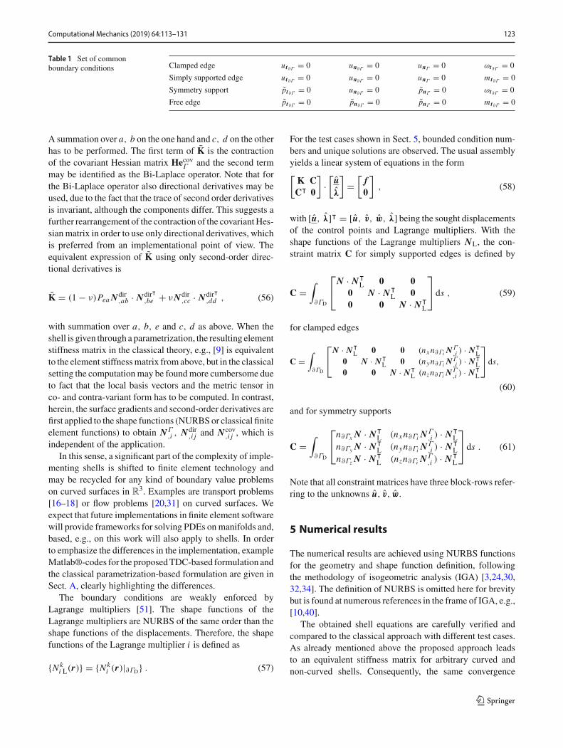
Table 1 Set of commonboundary conditions Clamped edge u t∂Γ

= 0 un∂Γ= 0 unΓ = 0 ωt∂Γ

= 0

Simply supported edge u t∂Γ= 0 un∂Γ

= 0 unΓ = 0 m t∂Γ= 0

Symmetry support pt∂Γ= 0 un∂Γ

= 0 pnΓ = 0 ωt∂Γ= 0

Free edge pt∂Γ= 0 pn∂Γ

= 0 pnΓ = 0 m t∂Γ= 0

A summation over a, b on the one hand and c, d on the otherhas to be performed. The first term of K is the contractionof the covariant Hessian matrix HecovΓ and the second termmay be identified as the Bi-Laplace operator. Note that forthe Bi-Laplace operator also directional derivatives may beused, due to the fact that the trace of second order derivativesis invariant, although the components differ. This suggests afurther rearrangement of the contraction of the covariantHes-sianmatrix in order to use only directional derivatives, whichis preferred from an implementational point of view. Theequivalent expression of K using only second-order direc-tional derivatives is

K = (1 − ν)PeaNdir,ab · Ndirᵀ

,be + νNdir,cc · Ndirᵀ

,dd , (56)

with summation over a, b, e and c, d as above. When theshell is given through a parametrization, the resulting elementstiffness matrix in the classical theory, e.g., [9] is equivalentto the element stiffnessmatrix from above, but in the classicalsetting the computationmay be foundmore cumbersome dueto fact that the local basis vectors and the metric tensor inco- and contra-variant form has to be computed. In contrast,herein, the surface gradients and second-order derivatives arefirst applied to the shape functions (NURBSor classical finiteelement functions) to obtain NΓ

,i , Ndir,i j and Ncov

,i j , which isindependent of the application.

In this sense, a significant part of the complexity of imple-menting shells is shifted to finite element technology andmay be recycled for any kind of boundary value problemson curved surfaces in R

3. Examples are transport problems[16–18] or flow problems [20,31] on curved surfaces. Weexpect that future implementations in finite element softwarewill provide frameworks for solving PDEs onmanifolds and,based, e.g., on this work will also apply to shells. In orderto emphasize the differences in the implementation, exampleMatlab®-codes for the proposedTDC-based formulation andthe classical parametrization-based formulation are given inSect. A, clearly highlighting the differences.

The boundary conditions are weakly enforced byLagrange multipliers [51]. The shape functions of theLagrange multipliers are NURBS of the same order than theshape functions of the displacements. Therefore, the shapefunctions of the Lagrange multiplier i is defined as

{Nki L(r)} = {Nk

i (r)|∂ΓD} . (57)

For the test cases shown in Sect. 5, bounded condition num-bers and unique solutions are observed. The usual assemblyyields a linear system of equations in the form[K CCᵀ 0

]·[uλ

]=

[f0

], (58)

with [u, λ]ᵀ = [u, v, w, λ] being the sought displacementsof the control points and Lagrange multipliers. With theshape functions of the Lagrange multipliers NL, the con-straint matrix C for simply supported edges is defined by

C =∫

∂ΓD

⎡⎣N · Nᵀ

L 0 00 N · Nᵀ

L 00 0 N · Nᵀ

L

⎤⎦ ds , (59)

for clamped edges

C =∫

∂ΓD

⎡⎣N · Nᵀ

L 0 0 (nxn∂Γi NΓ,i ) · Nᵀ

L0 N · Nᵀ

L 0 (nyn∂Γi NΓ,i ) · Nᵀ

L0 0 N · Nᵀ

L (nzn∂Γi NΓ,i ) · Nᵀ

L

⎤⎦ ds,

(60)

and for symmetry supports

C =∫

∂ΓD

⎡⎣n∂Γx N · Nᵀ

L (nxn∂Γi NΓ,i ) · Nᵀ

Ln∂Γy N · Nᵀ

L (nyn∂Γi NΓ,i ) · Nᵀ

Ln∂Γz N · Nᵀ

L (nzn∂Γi NΓ,i ) · Nᵀ

L

⎤⎦ ds . (61)

Note that all constraint matrices have three block-rows refer-ring to the unknowns u, v, w.

5 Numerical results

The numerical results are achieved using NURBS functionsfor the geometry and shape function definition, followingthe methodology of isogeometric analysis (IGA) [3,24,30,32,34]. The definition of NURBS is omitted here for brevitybut is found at numerous references in the frame of IGA, e.g.,[10,40].

The obtained shell equations are carefully verified andcompared to the classical approach with different test cases.As already mentioned above the proposed approach leadsto an equivalent stiffness matrix for arbitrary curved andnon-curved shells. Consequently, the same convergence

123


Fig. 6 Definition of flat shell problem

properties as shown, e.g., in [9,32] are expected. In the fol-lowing, the results of the convergence analyses of a flat shellembedded in R

3, the Scordelis-Lo roof, and the pinchedcylinder test (part of the shell obstacle course proposed byBelytschko et al. [2]) are shown. Furthermore, a new testcase with a challenging geometry is proposed which featuressmooth solutions enabling higher-order convergence rates.These rates are confirmed in the residual error as no analyticsolution exists, see Sect. 5.4. Other examples (e.g., pinchedhemispherical shell, shells of revolution, etc.) have been con-sidered but are omitted here for brevity.

In the convergence studies, NURBS patches with differ-ent orders and numbers of knot spans in each direction areemployed. This is equivalent to meshes with higher-orderelements and n = {2, 4, 8, 16, 32} elements per side areused. The orders are varied as p = {2, 3, 4, 5, 6}.

5.1 Flat shell embedded inR3

Following a similar rationale as in [27], as a first test case,we consider a simple quadrilateral, flat shell with the normalvector nΓ = [−1/4, −√

3/2,√3/4]ᵀ in R

3, see Fig. 6. Theshell is simply supported at all edges. For verification, the

Fig. 7 Displacement u of arbitrarily orientated flat shell, scaled by twoorders of magnitude a front view, b rotated view

load vector f is split into tangential f t and normal fn loads.The tangential loads are obtained with the method of man-ufactured solution for a given displacement field ut (x) =[ [1, 1]ᵀ · 1/4 · sin(πr) sin(πs)] ◦ χ−1. In normal direction,a sinusoidal load fn(x) = [−DB sin(πr) sin(πs)] ◦ χ−1

is applied to the shell. Herein, χ is an affine mappingfunction (rigid-body rotation) from the horizontal param-eter space to the real domain. An analytic solution forthe normal displacements is easily obtained with un(x) =[−(sin(πr) sin(πs))/(4π4)

]◦χ−1, [46]. The shell is definedwith L = 1 and the thickness is set to t = 0.01. The mate-rial parameters are: Young’s modulus E = 10000 and thePoisson’s ratio ν = 0.3.

In Fig. 7, the solution of the shell is illustrated. Thedisplacements are scaled by two orders of magnitude. Thecolours on the deformed surface indicate the Euclidean normof the displacement field ‖u‖.

The results of the convergence analysis are shown in Fig.8. The curves are plotted as a function of the element size 1/n

(which is rather a characteristic length of the knot spans). Thedotted lines indicate the theoretical optimal order of conver-gence. In Fig. 8a, the relative L2-error of the primal variable(displacements) is shown.Optimal higher-order convergencerates O(p + 1) are achieved. In the figures Fig. 8b–d, the

123


(a) (b)

(c) (d)

Fig. 8 Convergence results for the rotated flat shell. a Relative L2-norm of displacements u. b Relative L2-norm of normal forces nrealΓ . c RelativeL2-norm of bending momentsmΓ . d Relative L2-norm of transverse shear forces q

relative L2-errors of the normal forces (membrane forces),bending moments and transverse shear forces are plotted.For all stress resultants the theoretical optimal orders ofconvergence are achieved. It is clear that the same resultswere obtained if the results are computed for the purely two-dimensional case as, e.g., in [9].

5.2 Scordelis-Lo roof

The Scordelis-Lo roof is a cylindrical shell and is supportedwith two rigid diaphragms at the ends. The shell is loadedby gravity forces, see Fig. 9. The cylinder is defined withL = 50, R = 25 and the angle subtended by the roof isφ = 80◦. The thickness of the shell is set to t = 0.25. Thematerial parameters are: Young’s modulus E = 4.32 × 108

and the Poisson’s ratio ν = 0.0. In contrast to the first exam-

123


Fig. 9 Definition of Scordelis-Lo roof problem

ple, the maximum vertical displacement uz,max is comparedwith the reference solution uz,max,Ref = 0.3024 as given inreference [2].

In Fig. 10a, the numerical solution of the Scordelis-Loroof is illustrated. The displacements are magnified by oneorder of magnitude.

In Fig. 10b, the convergence of the maximum displace-ment uz,max is plotted up to polynomial order of p = 6 as afunction of the element (knot span) size. It is clearly seen thatthe expected results are achieved, with increasing accuracyfor higher-order NURBS. Due to the lack of a more accuratereference solutions, it is not useful to show these results ina double-logarithmic diagram as usual for error plots. Thestyle of presentation follows those of many other referencessuch as, e.g., in [2,9,32].

5.3 Pinched cylinder

The next test case is a cylindrical shell pinched with twodiametrically opposite unit loads located within the mid-dle of the shell, see Fig. 11. The cylinder is defined withL = 600, R = 300. The thickness is set to t = 3. The mate-rial properties are: Young’s modulus E = 3 × 106 and thePoisson’s ratio ν = 0.3. The reference displacement at theloading points are uRef = 1.82488 × 10−5 as given in refer-ence [2]. Due to symmetry only one eighth of the geometryis modelled.

In Fig. 12a, the numerical solution of the pinched cylinderis illustratedwith scaled displacements by a factor of 5×106.

(a)

(b)

Fig. 10 a Displacement field of the Lo-Scordelis roof scaled by oneorder of magnitude, b normalized convergence of reference displace-ment uz,max,Ref = 0.3024

As in the example before, in Fig. 12b, the convergence toa normalized reference displacement as a function of the ele-ment size is plotted. The results converge with the expectedbehaviour as shown in [9,32]. It is noted that due to the singu-larity in some mechanical quantities due to the single force,higher-order convergence rates are not possible here. How-ever, the improvement for increasing the order of theNURBSis still seen in the figure. An additional grading of the ele-ments in order to better resolve the singularity would havefurther improved the situation but is omitted here.

5.4 Flower shaped shell

As a last example, a more complex geometry is considered,which enables smooth mechanical fields and thereby enableshigher-order convergence rates. The geometry of the middlesurface is given with

123


Fig. 11 Definition of the pinched cylinder problem

xΓ (r , s) =⎡⎣

(A − C) cos(θ)

(A − C) sin(θ)

1 − s2

⎤⎦ (62)

with:

r , s ∈ [−1, 1] , A = 2.3 , B = 0.8

θ(r) = π(r + 1)

C(r , s) = s[B + 0.3 cos(6θ)](63)

and illustrated in Fig. 13. Below the figure, the boundaryconditions and material parameters are defined. The middlesurface of the shell features varying principal curvatures andcurved boundaries.

The curved boundaries are clamped and the correspondingconditions (from Table 1) have to be properly enforced. Ananalytical solution or reference displacement is not available.Therefore, the error is measured in the strong form of theequilibrium from Eq. (35) and may be called residual error.In particular, the residual error is the summed element-wiserelative L2-error

εrel,residual =nElem∑i=1

εL2,rel,τi

ε2L2,rel,τ =∫Γ

{divΓ nΓ + nΓ divΓ (P · divΓ mΓ )

+2H · divΓ mΓ + [∂xΓi H] jk [mΓ ]ki + f

}2

dΓ

∫Γ

f 2 dΓ.

(64)

(a)

(b)

Fig. 12 Pinched cylinder: a displacement u of one eighth of the geome-try (scaled by a factor of 5×106),bnormalized convergence of referencedisplacement uRadial,Ref = 1.82488 × 10−5 at loading points

The computation of the residual error requires the evaluationof fourth-order surface derivatives. It is noteworthy that theimplementation of these higher-order derivatives is not with-out efforts. For example, recall that mixed directional surfacederivatives are not symmetric. That is, there are 34 = 81partial fourth-order derivatives. Nevertheless, if the displace-ment field is smooth enough this error measure is a suitablequantity for the convergence analysis.

In Fig. 14a, the deformed shell is illustrated. The displace-ment field is scaled by one order of magnitude. In Fig. 14b,the results of the convergence analysis are plotted. Due tothe fact that fourth-order derivatives need to be computed,at least fourth-order shape functions are required. The the-oretical optimal order of convergence is O(p − 3) if thesolution is smooth enough. One may observe that higher-order convergence rates are achieved, however, rounding-offerrors and the conditioning may slightly influence the con-vergence. Nevertheless, the results are excellent also given

123


Fig. 13 Definition of flower shaped shell problem

the fact that higher-order accurate results for shells (given indouble-logarithmic error plots) are the exception.

The stored elastic energy at the finest level with a polyno-mial order p = 8, which may be seen as an overkill solution,is e = 1.7635958±1×10−7 kN m. This stored elastic energymay be used for future benchmark tests, without the need toimplement fourth-order derivatives on manifolds.

6 Conclusions and outlook

The linear Kirchhoff–Love shell theory is reformulated interms of the TDC using a global Cartesian coordinate systemand tensor notation. The resulting model equations apply toshell geometries which are parametrized or not. For example,a parametrizationmay not be availablewhen shell geometriesare implied by the level-set method. Because the TDC-basedformulation holds in both cases, it may be seen as a gen-eralization to the classical shell theory which is based onparametrizations and curvilinear coordinates.

The TDC-based strong form is used as the starting pointto consistently obtain the weak form including all boundarytermswell-known in the Kirchhoff–Love theory.Mechanicalstress-resultants such as moments, normal and shear forcesare defined in global coordinates. Furthermore, the strongformmaybeused in the numerical results to compute residualerrors and thus enable convergence analyses evenwithout theknowledge of exact solutions which, for shells, are scarce.

For the discretization, the Surface FEM is used withNURBS as trial and test functions. That is, an isogeometricapproach is chosen due to continuity requirements. In thiscase, the presence of a surface mesh (i.e., a NURBS patch),

(a)

(b)

Fig. 14 Flower shaped shell: a displacement u of flower shaped shell(scaled by one order of magnitude), b residual error εrel,residual

implies a parametrization and although the involved equa-tions and the resulting implementations vary significantly, itis seen that the classical, parametrization-based and the pro-posed TDC-based formulation are equivalent. For a genericfinite element framework enabling various implementationsfor PDEs on manifolds (in addition to only shells), the TDC-based approach is benefitial, because surface gradients ofshape functions may be computed beforehand and are inde-pendent of the application.

The numerical results confirm higher-order convergencerates. As mentioned, based on the residual errors, a frame-work for the verification of complex test cases is presented.There is a large potential in the parametrization-free refor-mulation of shell models, because the obtained PDEsmay bediscretizedwith new finite element techniques such as Trace-FEMor CutFEMbased on implicitly defined surfaces. In thiscase, neither the problem statement nor the discretization isbased on a parametrization.

123


Acknowledgements Open access funding provided byGrazUniversityof Technology.

Open Access This article is distributed under the terms of the CreativeCommons Attribution 4.0 International License (http://creativecommons.org/licenses/by/4.0/), which permits unrestricted use, distribution,and reproduction in any medium, provided you give appropriate creditto the original author(s) and the source, provide a link to the CreativeCommons license, and indicate if changes were made.

A Element stiffness matrix

In order to clarify the implementation, we give theMatlab�-code of the routine which evaluates the element contributionto the matrix and right hand side.

Using TDC, the input contains the shape function dataand normal vectors evaluated at the integration points plusthe material parameters, see Code 1. Note that the first- and

second-order surface derivatives are included in the shapefunction data, i.e., ∇Γ Ni (x j ) and Hecov(Ni (x j )) wherei = 1, . . . , n refers to the n shape functions in the currentelement (knot span) and x j with j = 1, . . . , m to integra-tion points. The computation of these quantities is part of thestandard finite element technology provided by the imple-mentation and is independent of the application to shells.

When curvilinear coordinates are used, the input containsshape function data, integration points, material parametersplus the coordinates of the control points of the correspond-ing element, see Code 2. Note that the included derivatives ofthe shape functions are the derivatives w.r.t. reference coordi-nates, i.e., ∇rN (r). As a first step, the covariant base vectorsand the metric tensor in co- and contra-variant form need tobe calculated at each integration point and in the next step,the element stiffness matrix and the element load vector arecomputed.

123

http://creativecommons.org/licenses/by/4.0/

http://creativecommons.org/licenses/by/4.0/


References

1. Basar Y, Krätzig WB (1985) Mechanik der Flächentragwerke.Vieweg+Teubner Verlag, Braunschweig

2. Belytschko T, Stolarski H, Liu WK, Carpenter N, Ong JSJ (1985)Stress projection for membrane and shear locking in shell finiteelements. Comput Methods Appl Mech Eng 51:221–258

3. Benson DJ, Bazilevs Y, HsuMC, Hughes TJR (2010) Isogeometricshell analysis: the Reissner–Mindlin shell. Comput Methods ApplMech Eng 199:276–289

4. BischoffM, Bletzinger KU,WallWA, RammE (2004)Models andfinite elements for thin-walledstructures, chapter 3. In: Encyclope-dia of computational mechanics. Wiley, Chichester

5. Blaauwendraad J, Hoefakker JH (2014) Structural shell analysis.Solid mechanics and its applications, vol 200. Springer, Berlin

6. Burman E, Claus S, Hansbo P, Larson MG, Massing A (2015)CutFEM: discretizing geometry and partial differential equations.Int J Numer Methods Eng 104:472–501

7. Burman E, Elfverson D, Hansbo P, Larson MG, Larsson K (2018)Shape optimization using the cut finite element method. ComputMethods Appl Mech Eng 328:242–261

8. Cenanovic M, Hansbo P, Larson MG (2016) Cut finite elementmodeling of linear membranes. Comput Methods Appl Mech Eng310:98–111

9. Cirak F, Ortiz M, Schröder P (2000) Subdivision surfaces: a newparadigm for thin-shell finite-element analysis. Int J Numer Meth-ods Eng 47(12):2039–2072

10. Cottrell JA, Hughes TJR, Bazilevs Y (2009) Isogeometric analysis:toward integration of CAD and FEA. Wiley, Chichester

11. DelfourMC,Zolésio JP (1994) Shape analysis via oriented distancefunctions. J Funct Anal 123:129–201

12. Delfour MC, Zolésio JP (1995) A boundary differential equationfor thin shells. J Differ Equ 119:426–449

13. Delfour MC, Zolésio JP (1996) Tangential differential equationsfor dynamical thin shallow shells. J Differ Equ 128:125–167

14. Delfour MC, Zolésio JP (1997) Differential equations for linearshells comparison between intrinsic and classical. In: Advancesin mathematical sciences: CRM’s 25 years (Montreal, PQ, 1994),Vol. 11 of CRM proceedings and lecture notes, Providence, RhodeIsland

15. Delfour MC, Zolésio JP (2011) Shapes and geometries: metrics,analysis, differential calculus, and optimization. SIAM, Philadel-phia

123


16. Demlow A (2009) Higher-order finite element methods and point-wise error estimates for elliptic problems on surfaces. SIAM JNumer Anal 47:805–827

17. Dziuk G (1988) Finite elements for the beltrami operator on arbi-trary surfaces: chapter 6. Springer, Berlin, pp 142–155

18. Dziuk G, Elliott CM (2013) Finite element methods for surfacePDEs. Acta Numer 22:289–396

19. Elfverson D, Larson MG, Larsson K (2018) A new least squaresstabilized Nitsche method for cut isogeometric analysis. ArXiv e-prints ArXiv:1804.05654

20. Fries TP (2018) Higher-order surface FEM for incompressibleNavier-Stokes flows on manifolds. Int J Numer Methods Fluids88:55–78. https://doi.org/10.1002/fld.4510

21. Fries TP, Omerovic S, Schöllhammer D, Steidl J (2017) Higher-order meshing of implicit geometries—part I: integration andinterpolation in cut elements. Comput Methods Appl Mech Eng313:759–784

22. Fries TP, SchöllhammerD (2017)Higher-ordermeshing of implicitgeometries—part II: approximations on manifolds. Comput Meth-ods Appl Mech Eng 326:270–297

23. Grande J, Reusken A (2016) A higher order finite element methodfor partial differential equations on surfaces. SIAM 54:388–414

24. GuoY, RuessM, Schillinger D (2017) A parameter-free variationalcoupling approach for trimmed isogeometric thin shells. ComputMech 59:693–715

25. Gurtin ME, Murdoch IA (1975) A continuum theory of elasticmaterial surfaces. Arch Ration Mech Anal 57:291–323

26. Hansbo P, Larson MG (2014) Finite element modeling of a lin-ear membrane shell problem using tangential differential calculus.Comput Methods Appl Mech Eng 270:1–14

27. Hansbo P, Larson MG (2017) Continuous/discontinuous finite ele-ment modelling of Kirchhoff plate structures inR3 using tangentialdifferential calculus. Comput Mech 60:693–702

28. Hansbo P, Larson MG, Larsson F (2015) Tangential differentialcalculus and the finite element modeling of a large deformationelastic membrane problem. Comput Mech 56:87–95

29. Hansbo P, Larson MG, Larsson K (2014) Variational formulationof curved beams in global coordinates. Comput Mech 53:611–623

30. Hughes TJR, Cottrell JA, Bazilevs Y (2005) Isogeometric analysis:CAD, finite elements, NURBS, exact geometry and mesh refine-ment. Comput Methods Appl Mech Eng 194:4135–4195

31. JankuhnT,OlshanskiiMA,ReuskenA (2017) Incompressible fluidproblems on embedded surfaces modeling and variational and for-mulations. ArXiv e-prints arXiv:1702.02989

32. Kiendl J, BletzingerK-U, Linhard J,Wüchner R (2009) Isogeomet-ric shell analysis with Kirchhoff–Love elements. Comput MethodsAppl Mech Eng 198:3902–3914

33. Lebiedzik C (2007) Exact boundary controllability of a shallowintrinsic shell model. J Math Anal Appl 335:584–614

34. Nguyen VP, Anitescu C, Bordas SPA, Rabczuk T (2015) Isogeo-metric analysis: anoverviewandcomputer implementation aspects.Math Comput Simul 117:89–116

35. Nguyen-Thanh N, Valizadeh N, Nguyen MN, Nguyen-Xuan H,Zhuang X, Areias P, Zi G, Bazilevs Y, Lorenzis L, De RabczukT (2015) An extended isogeometric thin shell analysis basedon Kirchhoff–Love theory. Comput Methods Appl Mech Eng284:265–291

36. Nguyen-Thanh N, Zhou K, Zhuang X, Areias P, Nguyen-XuanH, Bazilevs Y, Rabczuk T (2017) Isogeometric analysis of large-deformation thin shells using RHT-splines for multiple-patchcoupling. Comput Methods Appl Mech Eng 316:1157–1178

37. Olshanskii MA, Reusken A (2017) Trace finite element methodsfor PDEs on surfaces. In: Lecture notes in computational scienceand engineering, vol 121, pp 211–258

38. Olshanskii MA, Xu X (2017) A trace finite element method forPDEs on evolving surfaces. SIAM 39:A1301–A1319

39. Osher S, FedkiwRP (2003)Level setmethods anddynamic implicitsurfaces. Springer, Berlin

40. Piegl L, Tiller W (1997) The NURBS book (monographs in visualcommunication), 2nd edn. Springer, Berlin

41. Radwanska M, Stankiewicz A, Wosatko A, Pamin J (2017) Plateand shell structures. Wiley, Chichester

42. Reusken A (2014) Analysis of trace finite element methods forsurface partial differential equations. IMA J Numer Anal 35:1568–1590

43. Sethian JA (1999) Level set methods and fast marching methods,2nd edn. Cambridge University Press, Cambridge

44. Simo JC, Fox DD (1989) On a stress resultant geometricallyexact shell model—part I: formulation and optimal parametriza-tion. Comput Methods Appl Mech Eng 72:267–304

45. Simo JC, Fox DD, Rifai MS (1989) On a stress resultant geomet-rically exact shell model—part II: the linear theory; computationalaspects. Comput Methods Appl Mech Eng 73:53–92

46. Timoshenko S, Woinowsky-Krieger S (1959) Theory of plates andshells, 2nd edn. McGraw-Hill Book Company Inc, New York

47. van Opstal TM, van Brummelen EH, van Zwieten GJ (2015)A finite-element/boundary-element method for three-dimensional,large-displacement fluid structure-interaction. Comput MethodsAppl Mech Eng 284:637–663

48. Walker SW (2015) The shapes of things: a practical guide to differ-ential geometry and the shape derivative. Advances in design andcontrol. SIAM, Philadelphia

49. Wempner G, Talaslidis D (2002) Mechanics of solids and shells:theories and approximations. CRC Press, Boca Raton

50. Yao PF (2009) On shallow shell equations. Discret Contin DynSyst Ser S 2:697–722

51. ZienkiewiczO, TaylorR, Zhu JZ (2013) The finite elementmethod:its basis and fundamentals, 7th edn. Elsevier, Oxford

Publisher’s Note Springer Nature remains neutral with regard to juris-dictional claims in published maps and institutional affiliations.

123

http://arxiv.org/abs/ArXiv:1804.05654

https://doi.org/10.1002/fld.4510

http://arxiv.org/abs/arXiv:1702.02989

kirchhoff–love shell theory based on tangential

Documents