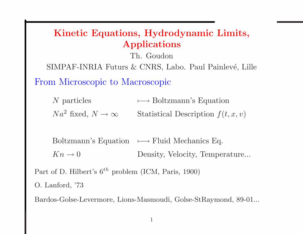
Kinetic Equations, Hydrodynamic Limits,Applications

Th. Goudon

SIMPAF-INRIA Futurs & CNRS, Labo. Paul Painleve, Lille

From Microscopic to Macroscopic

N particles 7−→ Boltzmann’s Equation

Na2 fixed, N → ∞ Statistical Description f(t, x, v)

Boltzmann’s Equation 7−→ Fluid Mechanics Eq.

Kn→ 0 Density, Velocity, Temperature...

Part of D. Hilbert’s 6th problem (ICM, Paris, 1900)

O. Lanford, ’73

Bardos-Golse-Levermore, Lions-Masmoudi, Golse-StRaymond, 89-01...

1

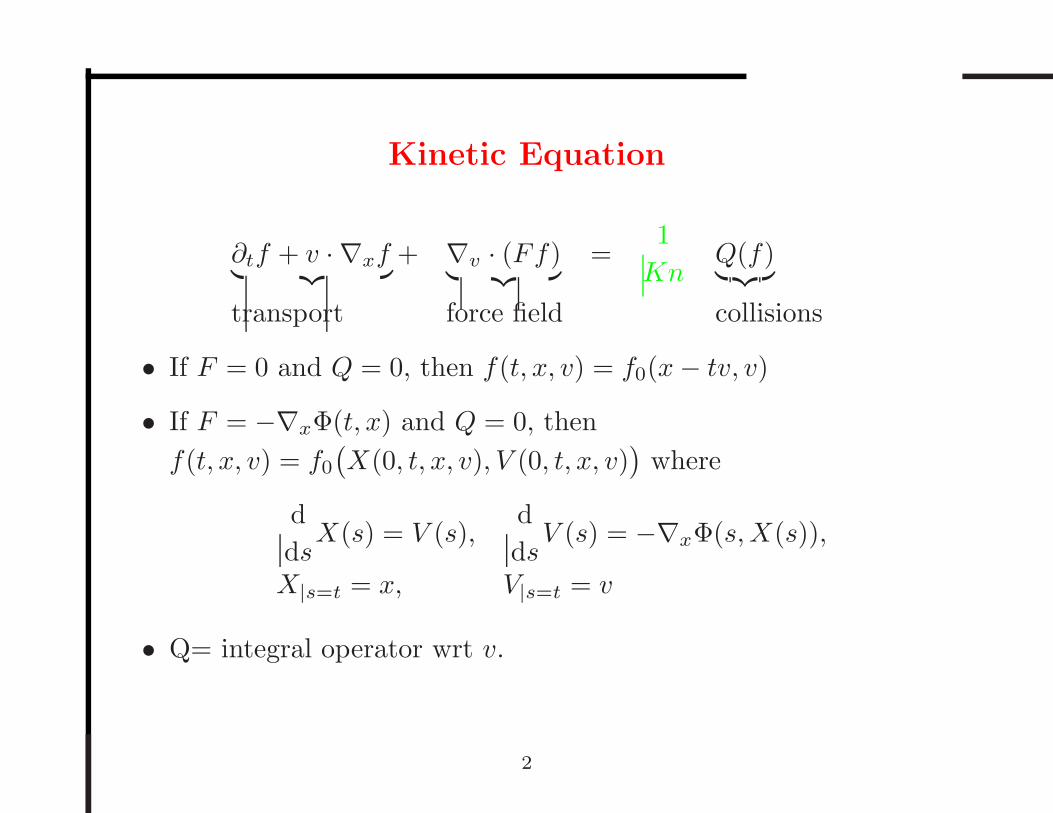
Kinetic Equation

∂tf + v · ∇xf︸ ︷︷ ︸

+ ∇v · (Ff)︸ ︷︷ ︸

=1

KnQ(f)︸ ︷︷ ︸

transport force field collisions

• If F = 0 and Q = 0, then f(t, x, v) = f0(x− tv, v)

• If F = −∇xΦ(t, x) and Q = 0, then

f(t, x, v) = f0(X(0, t, x, v), V (0, t, x, v)

)where

d

dsX(s) = V (s),

d

dsV (s) = −∇xΦ(s,X(s)),

X|s=t = x, V|s=t = v

• Q= integral operator wrt v.

2

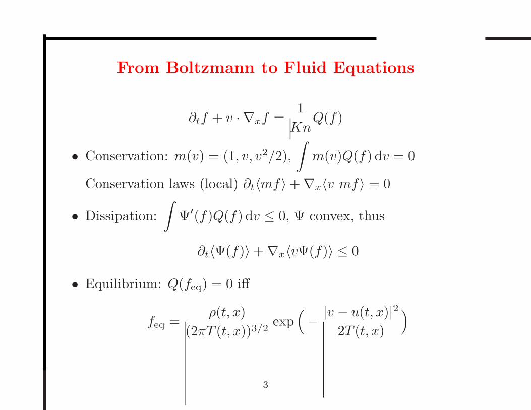
From Boltzmann to Fluid Equations

∂tf + v · ∇xf =1

KnQ(f)

• Conservation: m(v) = (1, v, v2/2),

∫

m(v)Q(f) dv = 0

Conservation laws (local) ∂t〈mf〉 + ∇x〈v mf〉 = 0

• Dissipation:

∫

Ψ′(f)Q(f) dv ≤ 0, Ψ convex, thus

∂t〈Ψ(f)〉 + ∇x〈vΨ(f)〉 ≤ 0

• Equilibrium: Q(feq) = 0 iff

feq =ρ(t, x)

(2πT (t, x))3/2exp

(

− |v − u(t, x)|22T (t, x)

)

3

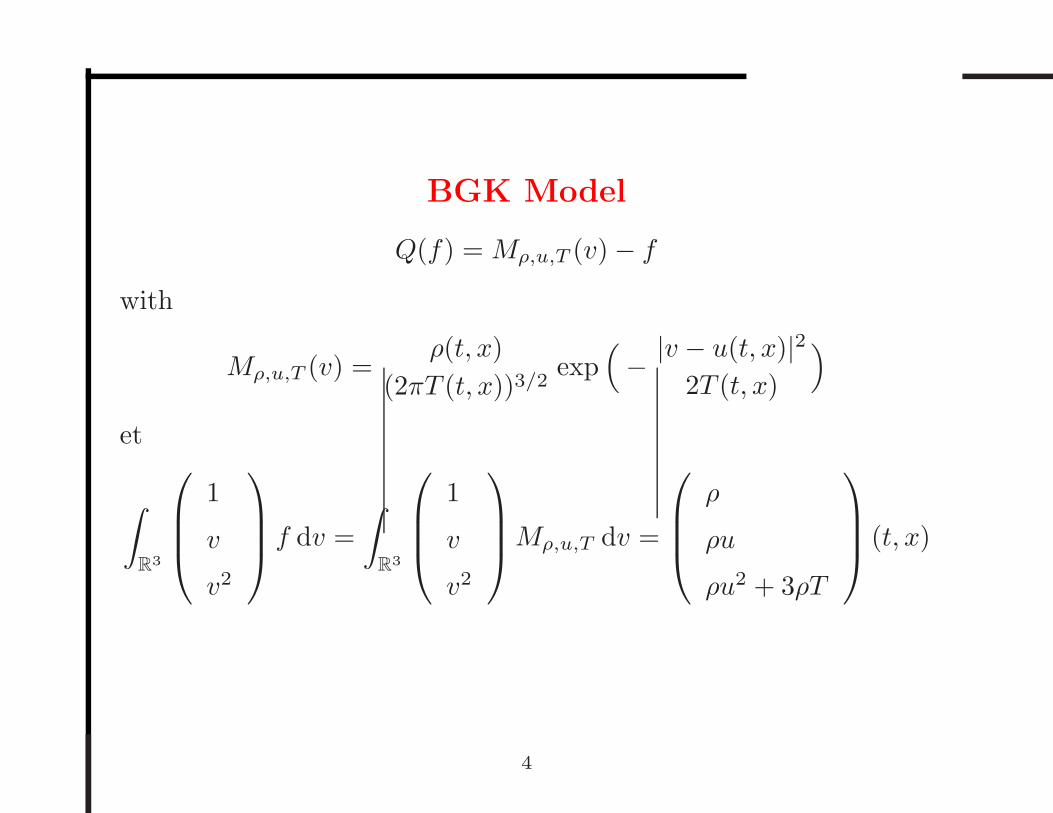
BGK Model

Q(f) = Mρ,u,T (v) − f

with

Mρ,u,T (v) =ρ(t, x)

(2πT (t, x))3/2exp

(

− |v − u(t, x)|22T (t, x)

)

et

∫

R3

1

v

v2

f dv =

∫

R3

1

v

v2

Mρ,u,T dv =

ρ

ρu

ρu2 + 3ρT

(t, x)

4

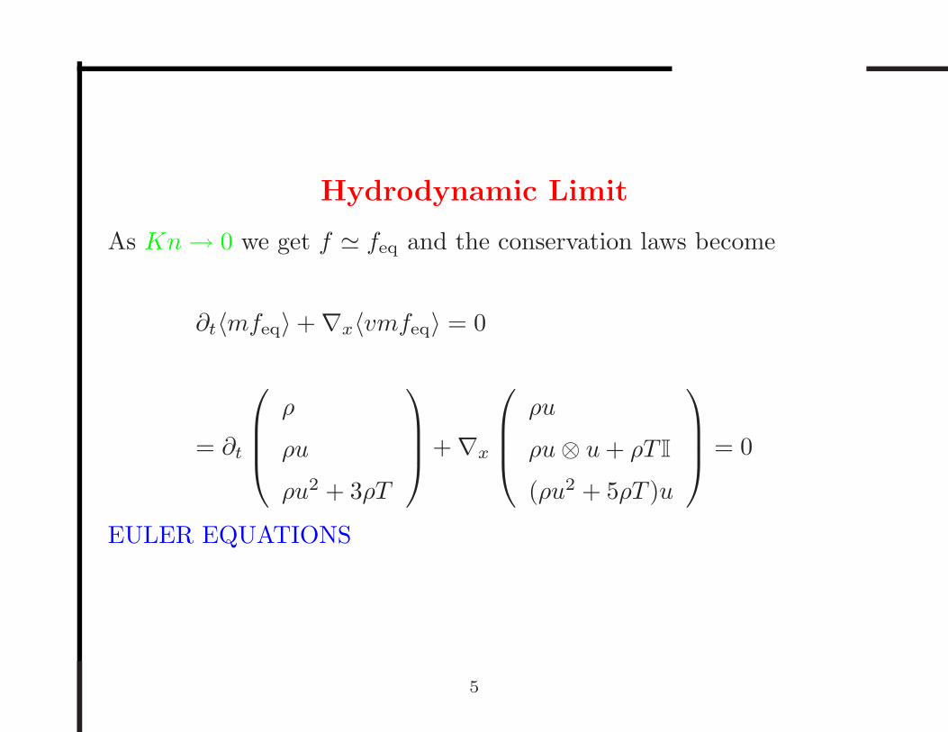
Hydrodynamic Limit

As Kn→ 0 we get f ≃ feq and the conservation laws become

∂t〈mfeq〉 + ∇x〈vmfeq〉 = 0

= ∂t

ρ

ρu

ρu2 + 3ρT

+ ∇x

ρu

ρu⊗ u+ ρT I

(ρu2 + 5ρT )u

= 0

EULER EQUATIONS

5

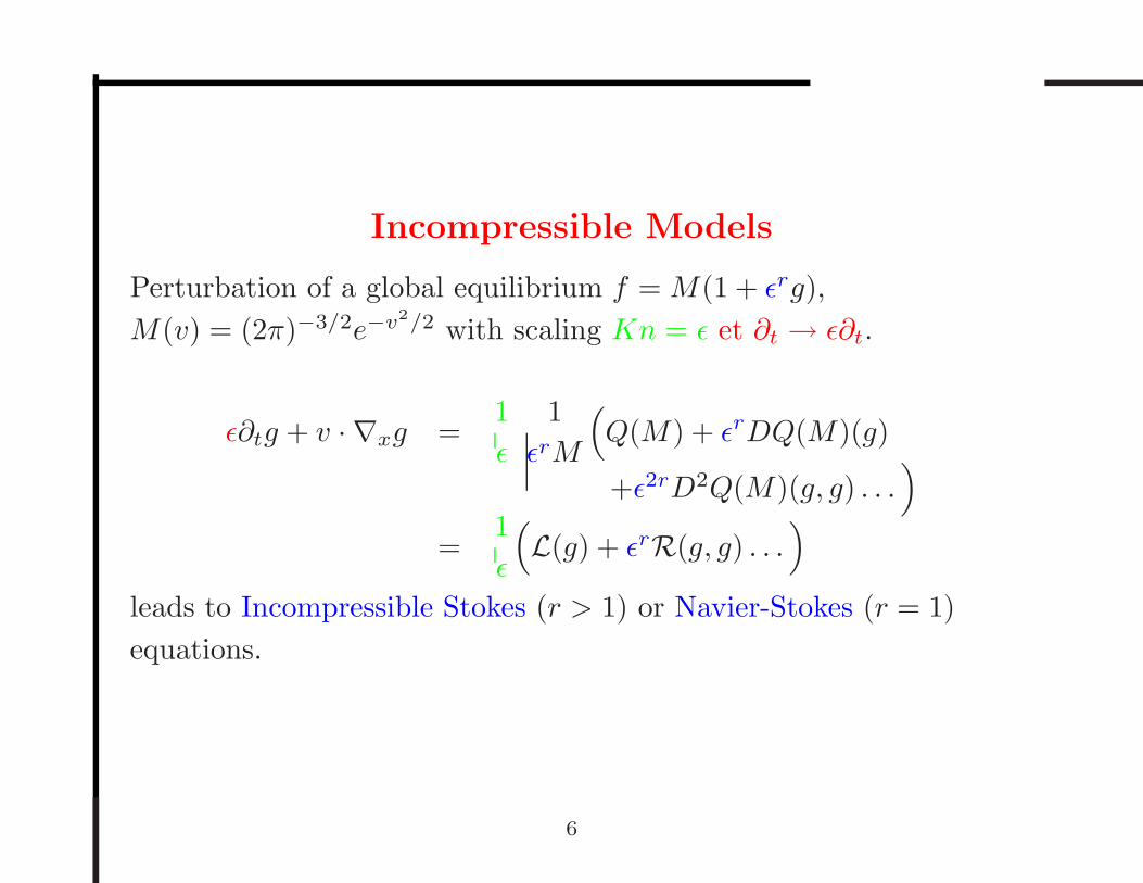
Incompressible Models

Perturbation of a global equilibrium f = M(1 + ǫrg),

M(v) = (2π)−3/2e−v2/2 with scaling Kn = ǫ et ∂t → ǫ∂t.

ǫ∂tg + v · ∇xg =1

ǫ

1

ǫrM

(

Q(M) + ǫrDQ(M)(g)

+ǫ2rD2Q(M)(g, g) . . .)

=1

ǫ

(

L(g) + ǫrR(g, g) . . .)

leads to Incompressible Stokes (r > 1) or Navier-Stokes (r = 1)

equations.

6

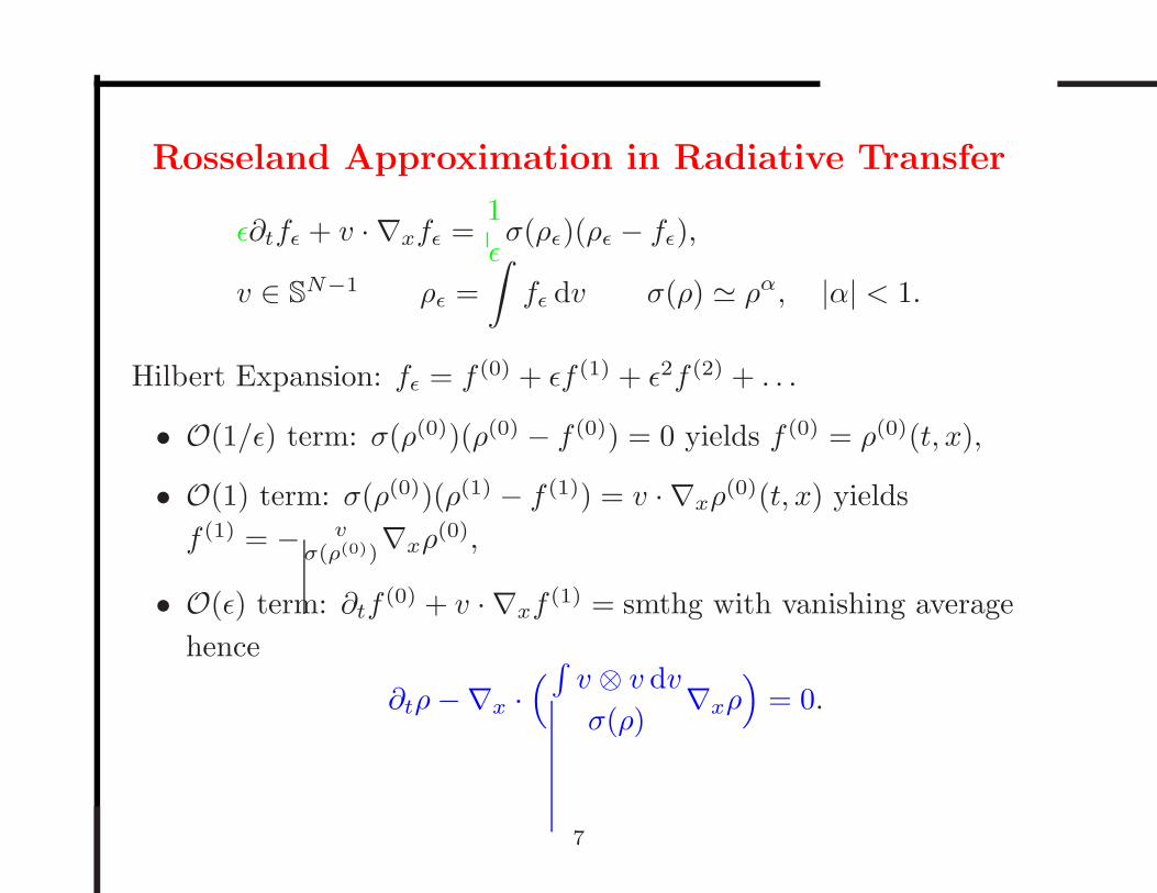
Rosseland Approximation in Radiative Transfer

ǫ∂tfǫ + v · ∇xfǫ =1

ǫσ(ρǫ)(ρǫ − fǫ),

v ∈ SN−1 ρǫ =

∫

fǫ dv σ(ρ) ≃ ρα, |α| < 1.

Hilbert Expansion: fǫ = f (0) + ǫf (1) + ǫ2f (2) + . . .

• O(1/ǫ) term: σ(ρ(0))(ρ(0) − f (0)) = 0 yields f (0) = ρ(0)(t, x),

• O(1) term: σ(ρ(0))(ρ(1) − f (1)) = v · ∇xρ(0)(t, x) yields

f (1) = − vσ(ρ(0))

∇xρ(0),

• O(ǫ) term: ∂tf(0) + v · ∇xf

(1) = smthg with vanishing average

hence

∂tρ−∇x ·(

∫v ⊗ v dv

σ(ρ)∇xρ

)

= 0.

7

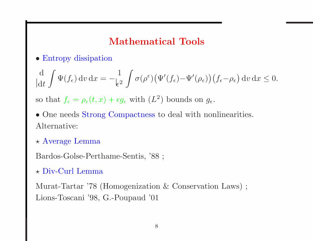
Mathematical Tools

• Entropy dissipation

d

dt

∫

Ψ(fǫ) dv dx = − 1

ǫ2

∫

σ(ρǫ)(Ψ′(fǫ)−Ψ′(ρǫ)

)(fǫ−ρǫ

)dv dx ≤ 0.

so that fǫ = ρǫ(t, x) + ǫgǫ with (L2) bounds on gǫ.

• One needs Strong Compactness to deal with nonlinearities.

Alternative:

⋆ Average Lemma

Bardos-Golse-Perthame-Sentis, ’88 ;

⋆ Div-Curl Lemma

Murat-Tartar ’78 (Homogenization & Conservation Laws) ;

Lions-Toscani ’98, G.-Poupaud ’01

8

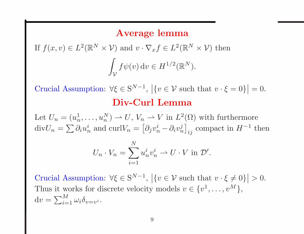
Average lemma

If f(x, v) ∈ L2(RN × V) and v · ∇xf ∈ L2(RN × V) then∫

V

fψ(v) dv ∈ H1/2(RN ).

Crucial Assumption: ∀ξ ∈ SN−1,∣∣v ∈ V such that v · ξ = 0

∣∣ = 0.

Div-Curl Lemma

Let Un = (u1n, . . . , u

Nn ) U , Vn V in L2(Ω) with furthermore

divUn =∑∂iu

in and curlVn =

[∂jv

in −∂iv

jn

]

ijcompact in H−1 then

Un · Vn =N∑

i=1

uinv

in U · V in D′.

Crucial Assumption: ∀ξ ∈ SN−1,∣∣v ∈ V such that v · ξ 6= 0

∣∣ > 0.

Thus it works for discrete velocity models v ∈ v1, . . . , vM,dv =

∑Mi=1 ωiδv=vi .

9

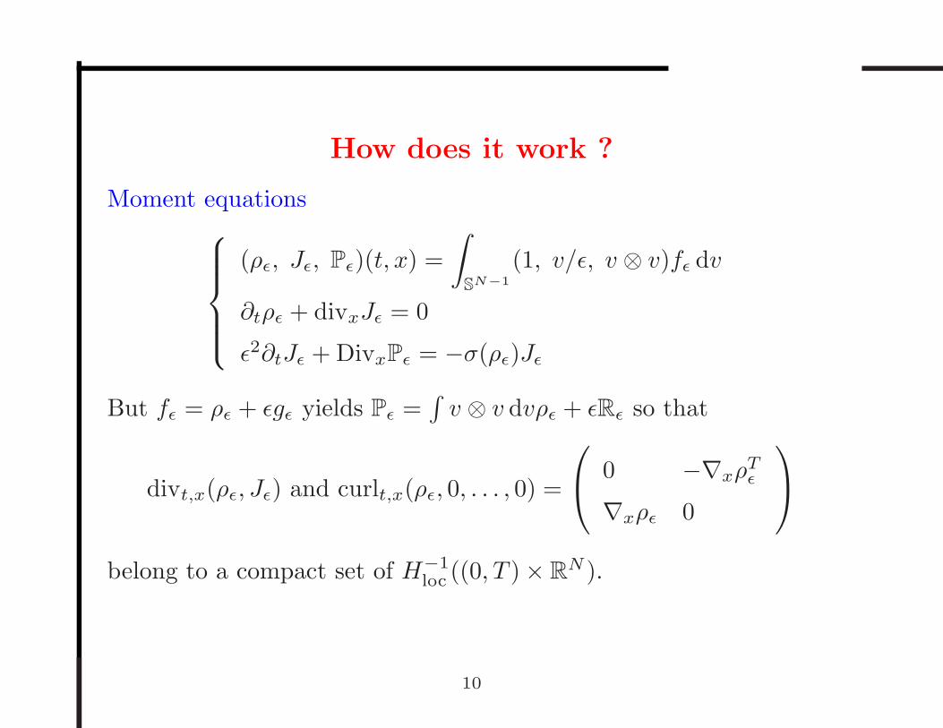
How does it work ?

Moment equations

(ρǫ, Jǫ, Pǫ)(t, x) =

∫

SN−1

(1, v/ǫ, v ⊗ v)fǫ dv

∂tρǫ + divxJǫ = 0

ǫ2∂tJǫ + DivxPǫ = −σ(ρǫ)Jǫ

But fǫ = ρǫ + ǫgǫ yields Pǫ =∫v ⊗ v dvρǫ + ǫRǫ so that

divt,x(ρǫ, Jǫ) and curlt,x(ρǫ, 0, . . . , 0) =

0 −∇xρ

Tǫ

∇xρǫ 0

belong to a compact set of H−1loc ((0, T ) × R

N ).

10

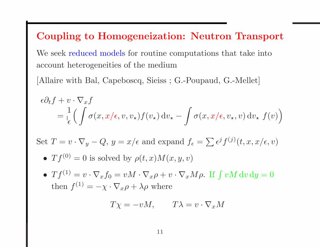
Coupling to Homogeneization: Neutron Transport

We seek reduced models for routine computations that take into

account heterogeneities of the medium

[Allaire with Bal, Capeboscq, Sieiss ; G.-Poupaud, G.-Mellet]

ǫ∂tf + v · ∇xf

=1

ǫ

(∫

σ(x, x/ǫ, v, v⋆)f(v⋆) dv⋆ −∫

σ(x, x/ǫ, v⋆, v) dv⋆ f(v))

Set T = v · ∇y −Q, y = x/ǫ and expand fǫ =∑ǫjf (j)(t, x, x/ǫ, v)

• Tf (0) = 0 is solved by ρ(t, x)M(x, y, v)

• Tf (1) = v · ∇xf0 = vM · ∇xρ+ v · ∇xMρ. If∫vM dv dy = 0

then f (1) = −χ · ∇xρ+ λρ where

Tχ = −vM, Tλ = v · ∇xM

11

Eventually, we get

∂tρ−∇x · (D(x)∇xρ− U(x)ρ) = 0,

D(x) =

∫ ∫

v ⊗ χ(x, y, v) dv dy, U(x) =

∫ ∫

vλ(x, y, v) dv dy

Convection term related to the space dependance of the

equilibrium function.

Degond-G.-Poupaud, 2003 ;

Chalub-Markowich-Perthame-Schmeiser, 2004

Treatment of the homogeneization aspect relies on double scale

technics∫

Ω

uǫψ(x, x/ǫ) dx −−−→ǫ→0

∫

(0,1)N

∫

Ω

Uψ(x, y) dxdy

12

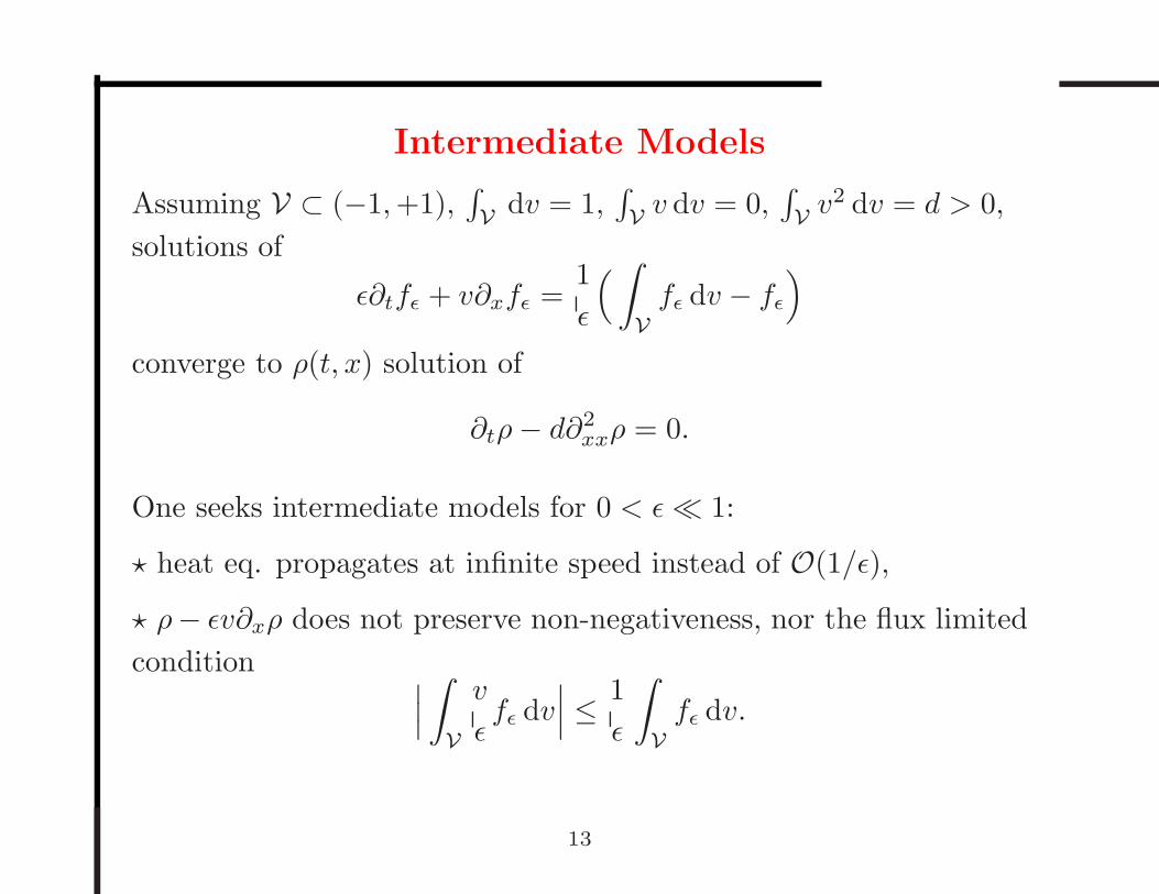
Intermediate Models

Assuming V ⊂ (−1,+1),∫

Vdv = 1,

∫

Vv dv = 0,

∫

Vv2 dv = d > 0,

solutions of

ǫ∂tfǫ + v∂xfǫ =1

ǫ

( ∫

V

fǫ dv − fǫ

)

converge to ρ(t, x) solution of

∂tρ− d∂2xxρ = 0.

One seeks intermediate models for 0 < ǫ≪ 1:

⋆ heat eq. propagates at infinite speed instead of O(1/ǫ),

⋆ ρ− ǫv∂xρ does not preserve non-negativeness, nor the flux limited

condition∣∣∣

∫

V

v

ǫfǫ dv

∣∣∣ ≤ 1

ǫ

∫

V

fǫ dv.

13

Minimum Entropy Principle Closure

The Moment System

∂tρǫ + divxJǫ = 0

ǫ2∂tJǫ + DivxPǫ = −Jǫ

is closed by imposing [Levermore ’97]

Pǫ =

∫

V

v2f⋆ǫ dv

where f⋆ǫ minimizes

∫

V

f ln f dv, with

∫

V

(1, v/ǫ)f dv = (ρǫ, Jǫ)

One obtains an hyperbolic system Pǫ = ρǫψ(ǫJǫ/ρǫ) which is

globally well-posed for small enough initial data, and consistent to

the diffusion eq. as ǫ goes to 0. [Coulombel-Golse-G.’06]

14

Astrophysics

Diffusion regimes might lead to singularity phenomena!

Vlasov-Poisson-Fokker-Planck Equation

ǫ∂tf + v · ∇xf −∇xΦ · ∇vf =1

ǫ∇v · (vf + ∇vf)

=1

ǫ∇v · (M∇v(f/M))

with M(v) = (2π)−N/2 e−v2/2 coupled to ∆Φ = ρ

For small ǫ’s, we guess [Chandrasekhar, 1943] f ≃ ρ(t, x)M(v)

where ρ satisfies

∂tρ−∇x · (∇xρ+ ρ∇xΦ) = 0, ∆Φ = ρ

Smoluchowski eq (or Keller-Segel in biology)

Competition between diffusion and Ricatti’s like behavior

∂tρ−∇xΦ · ∇xρ = ρ∆xΦ = ρ2

15

2D Case

Threshold phenomena: If∫

R2 ρ20 < M⋆ then global existence of

“smooth” solutions, If∫

R2 ρ20 > M⋆, formation of Dirac mass in

finite time.

Beckner, Carlen-Loss estimate (’92): Let ρ ≥ 0 and∫

R2 ρ dx = 1

then

−4

∫

R2

∫

R2

ρ(x)ρ(y) ln(|x− y|)dy dx ≤ C∗ + 2

∫

R2

ρ ln(ρ) dx.

Entropy estimate

d

dt

∫

R4

fǫ

(ln(fǫ)+

v2

2+Φǫ

)dv dx ≤ − 4

ǫ2

∫

R4

∣∣∇v

√

fǫ/M∣∣2M dv dx.

Global convergence ǫ→ 0 in the subcritical case [G.’06].

Numerics based on DG methods [Gamba-G.-Proft]

16

Fluid/Particles Flows

Applications: Rocket Propulsors, Diesel Engines, Steel Production

Processes...

∂tf + v · ∇xf −∇xU · ∇vf + ∇v · ((u− v)f) = ∆vf

Modeling discussions: Viscosity, Incompressibiliy,

Coagulation-fragmentation...

Identification of Relevant Parameters and Asymptotic Regimes:

e. g. Stokes settling time ≪ observation time leads to

Hydrodynamic Limits, but the regime also depends on ρp/ρg...

Turbulent Flows

Given u with high and fast random variations

Behavior of lim...

⟨f⟩

? [G.Poupaud 04]:

Diffusion-convection/Convection/Fokker-Planck

17

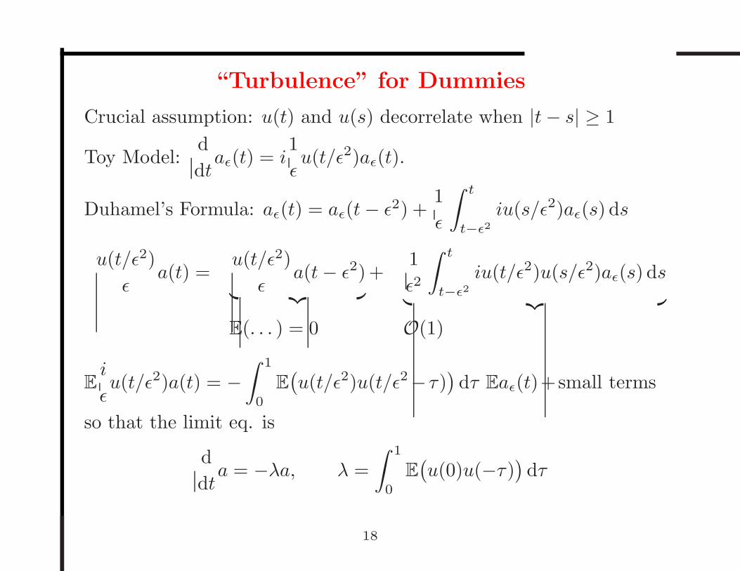
“Turbulence” for Dummies

Crucial assumption: u(t) and u(s) decorrelate when |t− s| ≥ 1

Toy Model:d

dtaǫ(t) = i

1

ǫu(t/ǫ2)aǫ(t).

Duhamel’s Formula: aǫ(t) = aǫ(t− ǫ2) +1

ǫ

∫ t

t−ǫ2iu(s/ǫ2)aǫ(s) ds

u(t/ǫ2)

ǫa(t) =

u(t/ǫ2)

ǫa(t− ǫ2)

︸ ︷︷ ︸

+1

ǫ2

∫ t

t−ǫ2iu(t/ǫ2)u(s/ǫ2)aǫ(s) ds

︸ ︷︷ ︸

E(. . . ) = 0 O(1)

Ei

ǫu(t/ǫ2)a(t) = −

∫ 1

0

E(u(t/ǫ2)u(t/ǫ2−τ)

)dτ Eaǫ(t)+small terms

so that the limit eq. is

d

dta = −λa, λ =

∫ 1

0

E(u(0)u(−τ)

)dτ

18

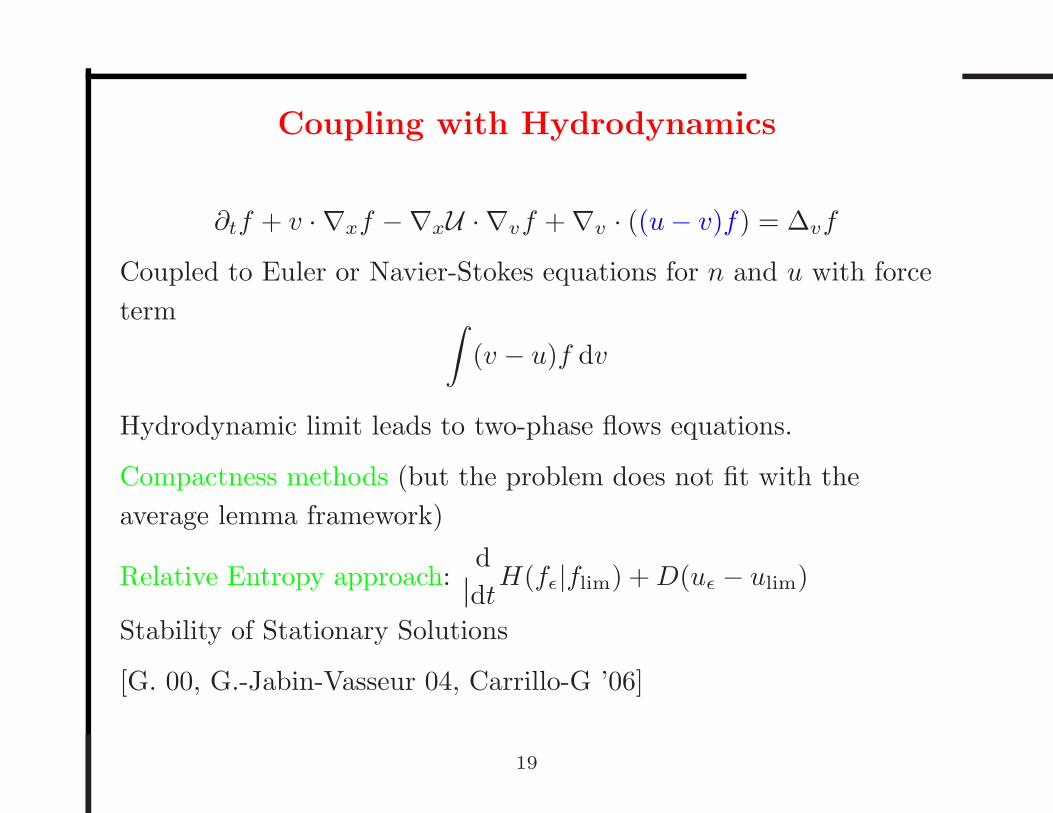
Coupling with Hydrodynamics

∂tf + v · ∇xf −∇xU · ∇vf + ∇v · ((u− v)f) = ∆vf

Coupled to Euler or Navier-Stokes equations for n and u with force

term ∫

(v − u)f dv

Hydrodynamic limit leads to two-phase flows equations.

Compactness methods (but the problem does not fit with the

average lemma framework)

Relative Entropy approach:d

dtH(fǫ|flim) +D(uǫ − ulim)

Stability of Stationary Solutions

[G. 00, G.-Jabin-Vasseur 04, Carrillo-G ’06]

19

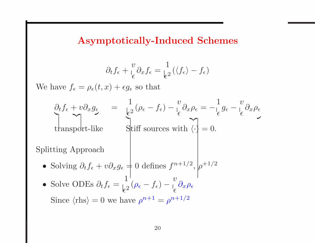
Asymptotically-Induced Schemes

∂tfǫ +v

ǫ∂xfǫ =

1

ǫ2(〈fǫ〉 − fǫ)

We have fǫ = ρǫ(t, x) + ǫgǫ so that

∂tfǫ + v∂xgǫ︸ ︷︷ ︸

=1

ǫ2(ρǫ − fǫ) −

v

ǫ∂xρǫ = −1

ǫgǫ −

v

ǫ∂xρǫ

︸ ︷︷ ︸

transport-like Stiff sources with 〈·〉 = 0.

Splitting Approach

• Solving ∂tfǫ + v∂xgǫ = 0 defines fn+1/2, ρ+1/2

• Solve ODEs ∂tfǫ =1

ǫ2(ρǫ − fǫ) −

v

ǫ∂xρǫ

Since 〈rhs〉 = 0 we have ρn+1 = ρn+1/2

20

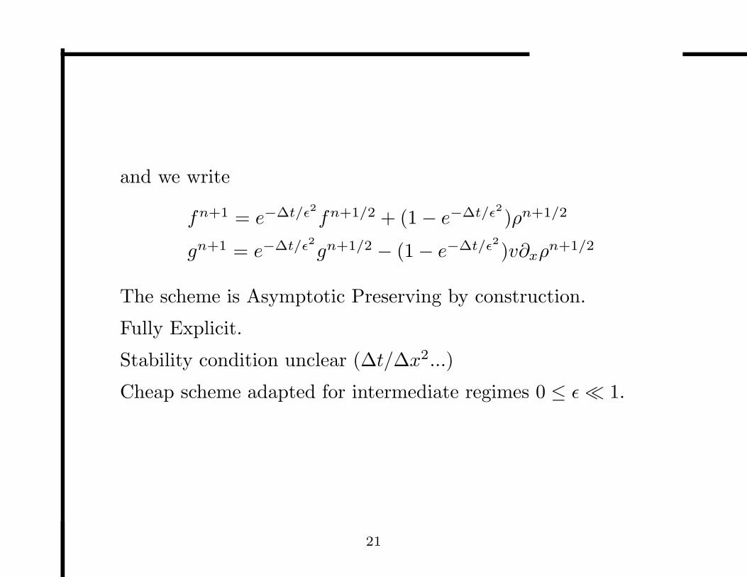
and we write

fn+1 = e−∆t/ǫ2fn+1/2 + (1 − e−∆t/ǫ2)ρn+1/2

gn+1 = e−∆t/ǫ2gn+1/2 − (1 − e−∆t/ǫ2)v∂xρn+1/2

The scheme is Asymptotic Preserving by construction.

Fully Explicit.

Stability condition unclear (∆t/∆x2...)

Cheap scheme adapted for intermediate regimes 0 ≤ ǫ≪ 1.

21

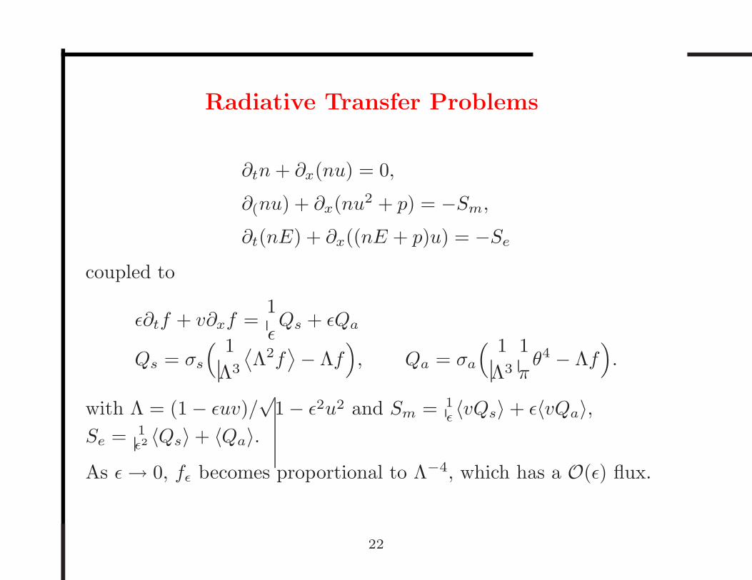
Radiative Transfer Problems

∂tn+ ∂x(nu) = 0,

∂(nu) + ∂x(nu2 + p) = −Sm,

∂t(nE) + ∂x((nE + p)u) = −Se

coupled to

ǫ∂tf + v∂xf =1

ǫQs + ǫQa

Qs = σs

( 1

Λ3

⟨Λ2f

⟩− Λf

)

, Qa = σa

( 1

Λ3

1

πθ4 − Λf

)

.

with Λ = (1 − ǫuv)/√

1 − ǫ2u2 and Sm = 1ǫ 〈vQs〉 + ǫ〈vQa〉,

Se = 1ǫ2 〈Qs〉 + 〈Qa〉.

As ǫ→ 0, fǫ becomes proportional to Λ−4, which has a O(ǫ) flux.

22

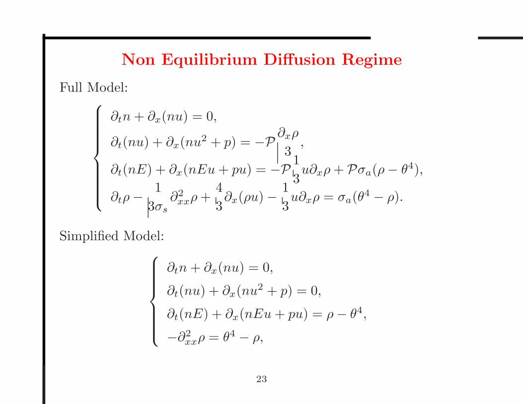
Non Equilibrium Diffusion Regime

Full Model:

∂tn+ ∂x(nu) = 0,

∂t(nu) + ∂x(nu2 + p) = −P ∂xρ

3,

∂t(nE) + ∂x(nEu+ pu) = −P 1

3u∂xρ+ Pσa(ρ− θ4),

∂tρ−1

3σs∂2

xxρ+4

3∂x(ρu) − 1

3u∂xρ = σa(θ4 − ρ).

Simplified Model:

∂tn+ ∂x(nu) = 0,

∂t(nu) + ∂x(nu2 + p) = 0,

∂t(nE) + ∂x(nEu+ pu) = ρ− θ4,

−∂2xxρ = θ4 − ρ,

23

Questions are related to the effects of the Energy Exchanges on the

features of the usual Euler system:

- Smoothing effects on the shock profile [Lin-Coulombel-G. ’06]

- Stability questions (of constants, of shocks profiles...)

- Asymptotic problems [G.-Lafitte ’06]

- Numerical Experiments

24