2/4/2005

Hydrodynamic Self Consistent Field Theory:Viscoelastic Microphase Separation

of Diblock Copolymers

David M. Hall LANL T-11 & UCSB Dept. of PhysicsSanjoy Banerjee UCSB, Dept. Chemical EngineeringTurab Lookman LANL Theoretical Division

Hydrodynamic Self Consistent Field Theory:Viscoelastic Microphase Separation

of Diblock Copolymers

HSCFT Overview• HSCFT extends Self Consistent Field Theory to non-equilibrium, hydrodynamic flows

SCFT Diblock Thermodynamic

Model

SCFT Diblock Thermodynamic

Model

“Two Fluid”Hydrodynamic

Model

“Two Fluid”Hydrodynamic

Model

Chemical Potential Gradients

Monomer Concentrations

LTELoop

10−12 −10−9 sec 10−3 −102 sec

Constitutive EquationConstitutive Equation

2/4/2005

Diblock Thermodynamic Model

• Mean field Free Energy

• Local thermal equilibrium conditions

• Monomer concentrations matched by steepest ascent

• Non-equilibrium chemical potentials

F = E − T(SJ + SA + SB )

δFδωA

=nkTV

˜ φ A − φ[ ]= 0 δFδωB

=nkTV

˜ φ B − (1− φ)[ ]= 0

µ = v0δFδφ

=kTN

χN 1− 2φ( )+ ωB −ωA[ ]

ω in +1 = ω i

n + λ δFδω i

˜ φ A =1Q

dsqq+0f∫

Q =1V

drq r,s( )∫ q+ r,s( )

∂q∂s

=Nb2

2d∇2q −ωq

˜ φ B =1Q

dsqq+f1∫

EnkT

= +1V

dr∫ Nχφ 1− φ( )

SA

nk= −

1V

dr∫ ρJ lnq + φωA( )

SB

nk= −

1V

dr∫ ρJ lnq+ + 1−φ( )ωB( )

SJ

nk= +

1V

dr∫ ρJ lnρJ

2/4/2005

Two Fluid Hydrodynamic Model

• Incompressibility

• Monomer Conservation

• Relative Velocity Force Balance

• Momentum Conservation

∇ ⋅ v = 0

∂tφ = −∇ ⋅ φvA( )

w =1

ζ φ( )−φ 1− φ( )∇µ[ ]+ a φ( )∇ ⋅ σ (n )

ρ∂tv = −φ∇µ + ∇ ⋅ σ (n ) − ∇p

v = φvA + 1− φ( )vB

ζ φ( )=ζ Aζ B

ζ A + ζ B

a φ( )= 1− φ( )αA − φαB

α i =ζ i

ζA + ζ B

ζ i = φ N /Ne( )ζ 0i

w = vA − vB

2/4/2005

Linear Maxwell Constitutive Equations

• Shear stress evolution

• Bulk stress evolution

• Concentration dependant moduli

• Stress relaxation times

∂tσ b( i) = −σ b

(i) /τ b(i) φ( )+ K ( i) φ( ) ∇ ⋅ vT( )δ

∂tσ S( i) = −σ S

(i) /τ S(i) φ( )+ G( i) φ( )κT

GA φ( )= G0Aφ 2 K A φ( )= K0

Aθ φ − f( )K B φ( )= K0

Bθ f − φ( )GB φ( )= G0B 1− φ( )2

τ S(i) φ( )= τ S

( i) τ b(i) φ( )= τ b

( i)

κTij = ∂ivT

j + ∂ jvTi −

2D

∇ ⋅ vT( )

vT = αA vA + αB vB

σ (n ) = σ bA + σ b

B + σ SA + σ S

B

2/4/2005

Results• 2D morphology vs. time• W and V curves are most useful for tracking important events• Micro-phase separation consists of three distinct stages

– Early stage has exponential growth– Intermediate stage characterized by rapid transition to defect filled morphology– Late stage characterized by long, slow process of defect reduction and annihilation

events• After very long times, morphologies approach equilibrium states• Length of exponential growth phase has a simple functional form in f• Shearing flows and bulk flows are both important.• Each entropy component has two distinct decay times.• 3D structures are highly defect filled, but correlate well with phase diagram.• Euler characteristics are most useful quantity for classifying 3D structures.• Viscoelastic phase separation occurs much as it does for blends, but with a more

structured network• Junction densities grow exponentially, and are expelled from each phase as it separates.• Viscoelastic phase separation in 3D

2/4/2005

2/4/2005

Time evolution of Morphology vs. f, 2D

f = 0.30

f = 0.35

f = 0.25

f = 0.50

f = 0.45

f = 0.40

time

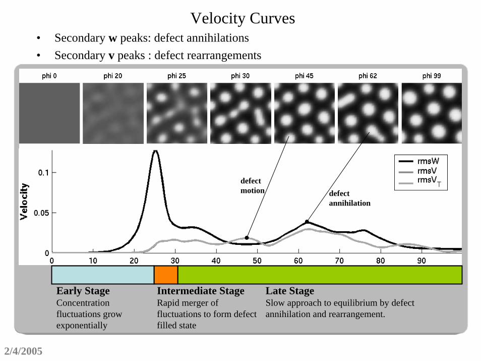
Velocity Curves• Secondary w peaks: defect annihilations• Secondary v peaks : defect rearrangements

defectmotion defect

annihilation

Early StageConcentration fluctuations grow exponentially

Late StageSlow approach to equilibrium by defect annihilation and rearrangement.

Intermediate StageRapid merger of fluctuations to form defect filled state

2/4/2005

Phase Separation Time vs. f• Structure growth time diverges as f approaches the ODT

twmax ∝1

f − f0( )α 1− f − f0( )α

Giτ i = 0.100f0 = 0.222α =1.30

tmax(w )

f

Giτ i = 0.001f0 = 0.235α =1.00

2/4/2005

Phase Separation Movies, 2D

2/4/2005

QuickTime™ and a decompressor

are needed to see this picture.

f = 0.30

QuickTime™ and a decompressor

are needed to see this picture.

f = 0.40

QuickTime™ and a decompressor

are needed to see this picture.

f = 0.35

f = 0.45 f = 0.50

Minority Block Morphology vs. Time, 3Df = 0.25

f = 0.30

f = 0.35

f = 0.50

2/4/2005

2/4/2005

Equilibrium Phase Diagram

A B C D

f

Nχ

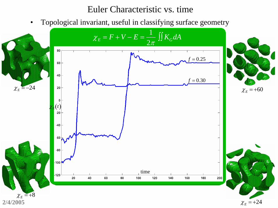
Euler Characteristic vs. time• Topological invariant, useful in classifying surface geometry

2/4/2005 χE = +24

χE = +60χE = −24

χE = +8

χE t( )

time

f = 0.30

f = 0.25

χE = F + V − E =1

2πKGdA∫∫

2/4/2005

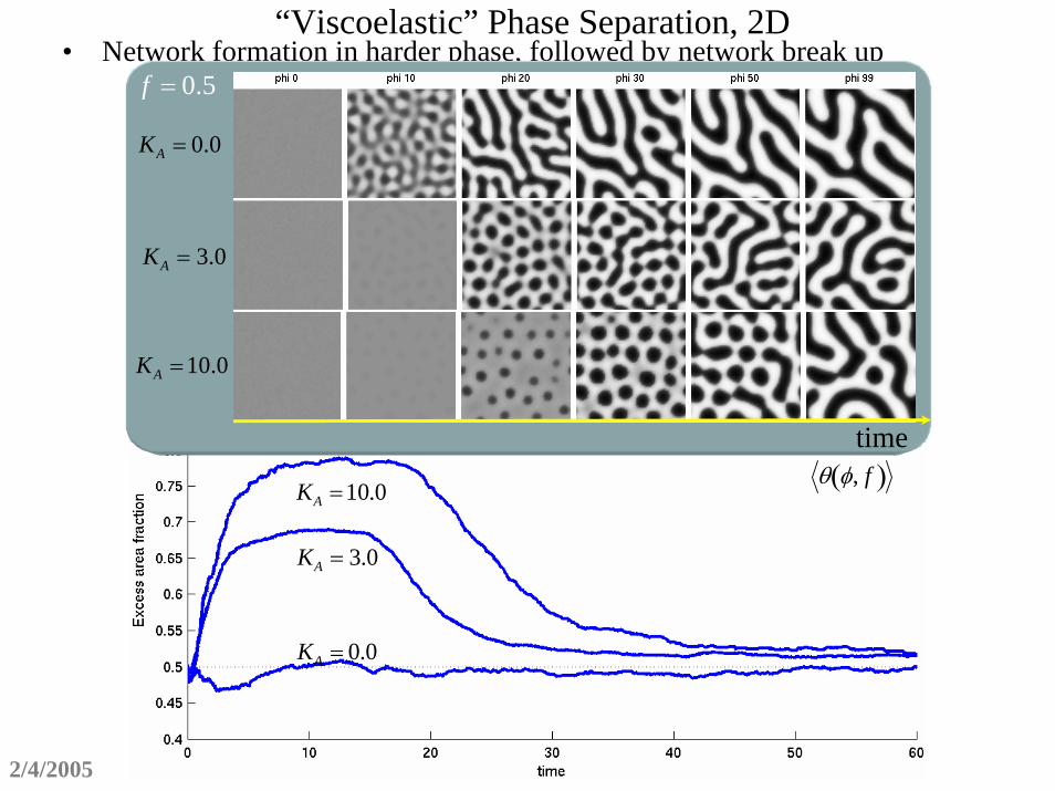
“Viscoelastic” Phase Separation, 2D

KA = 3.0

KA =10.0

KA = 0.0

• Network formation in harder phase, followed by network break up

θ φ, f( )

KA = 3.0

KA =10.0

KA = 0.0

f = 0.5

time

2/4/2005

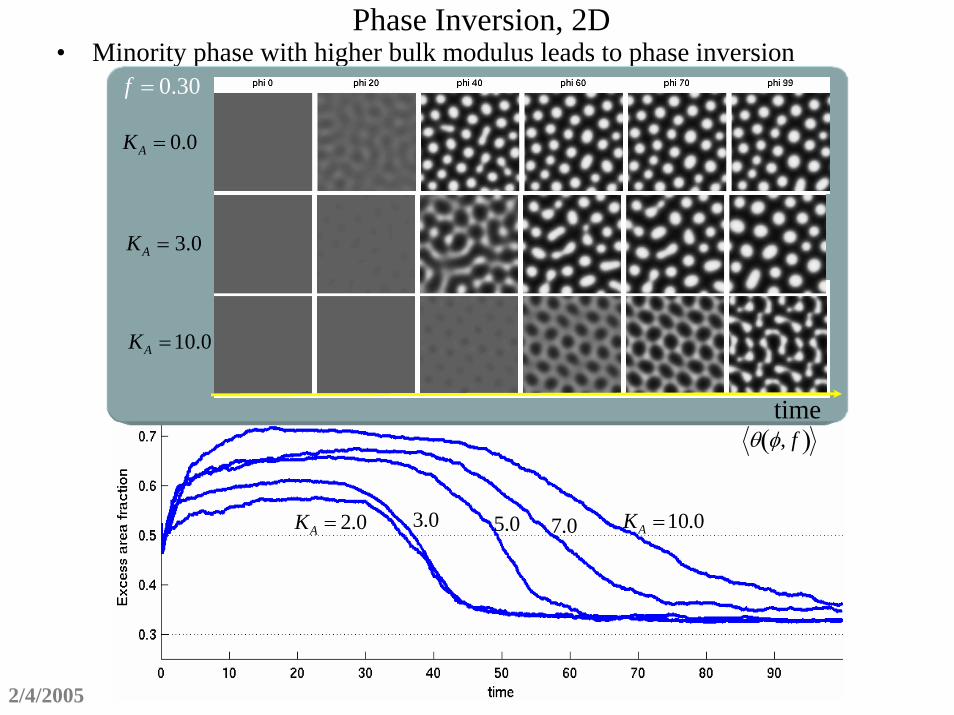
Phase Inversion, 2D• Minority phase with higher bulk modulus leads to phase inversion

3.0 KA =10.0KA = 2.0 5.0 7.0

θ φ, f( )

KA = 3.0

KA =10.0

KA = 0.0

f = 0.30

time

Viscoelastic Phase Separation,3D

f = 0.30KA = 5.0

f = 0.25KA = 5.0

f = 0.30KB = 5.0

f = 0.30

2/4/2005

EVF and Euler Curves, 3D Visco.

f = 0.30KA = 5.0

f = 0.30KB = 5.0

f = 0.25KA = 5.0

Evf vs. time

f = 0.30KA = 5.0

Euler Characteristic vs. time

2/4/2005

2/4/2005

Viscoelastic Phase Separation Movies, 3Df = 0.30 f = 0.30 KA = 5.0 f = 0.30 KB = 5.0

QuickTime™ and a decompressor

are needed to see this picture.

QuickTime™ and a decompressor

are needed to see this picture.

QuickTime™ and a decompressor

are needed to see this picture.

f = 0.25 KA = 5.0

AB Junction Densities vs. Time, 2DKA = 0.0,KB = 0.0

φ

ρJ

KA =10.0,KB = 0.0

φ

ρJ

2/4/2005

AB Junction Distribution vs. Time

1−< ρJ

2ψ 2 ><ψ 2 >

ψ ≡ φ − f

KA =10.0KA = 0.0

KA =10.0

KA = 0.0

ρJψ

AB Junction BiasA

B

2/4/2005

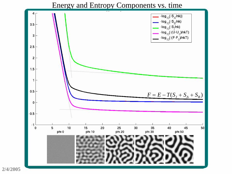
Energy and Entropy Components vs. time

F = E − T(SJ + SA + SB )

2/4/2005

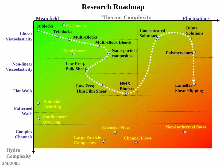
Research RoadmapMean field Fluctuations

LinearViscoelasticity

Non-linearViscoelasticity

Thermo-Complexity

Hydro Complexity

Complex Channels

Patterned Walls

Diblocks

Multi-BlocksMulti-Block Blends

Nano-particlecomposites

Flat Walls

Tri-blocksDilute Solutions

Polymersomes

Low Freq.Bulk Shear

Low Freq.Thin Film Shear

ConcentratedSolutions

Dendrimers

Confinement Ordering

EpitaxialOrdering

Extrusive Flow Non-isothermal flows

LamellarShear Flipping

Cyclomers

Channel FlowsLarge ParticleComposites

HMXBinders

2/4/2005

Future Research Directions• Examine more complex thermodynamic models

– Multi-block copolymers– Copolymer Blends– Particle, Block Nano-composites– Copolymer solutions, Polymersomes– Highly branched copolymers– Thermal fluctuations: Monte-Carlo sampling of partition function

• Examine more complex hydrodynamic flows:– Shearing flows: thin film shear and bulk shear flows– Verify shear flipping phenomenon?– Phase separation in presence of complex boundaries– Patterned Boundaries– Secondary flows in pressure driven channel simulations

• Extend ability to measure bulk material properties– Material strength vs. various deformations

• Automate adjustment of cell size to minimize external pressure effects

2/4/2005

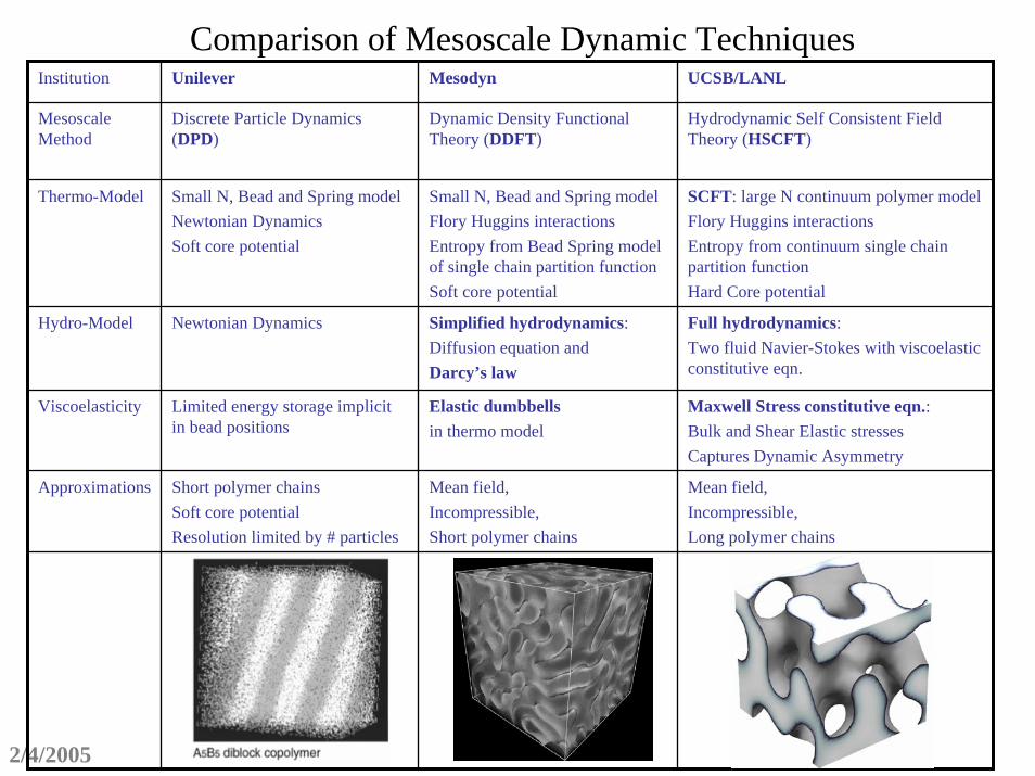
Comparison of Mesoscale Dynamic TechniquesInstitution Unilever Mesodyn UCSB/LANL

Mesoscale Method

Discrete Particle Dynamics (DPD)

Dynamic Density Functional Theory (DDFT)

Hydrodynamic Self Consistent Field Theory (HSCFT)

Thermo-Model Small N, Bead and Spring modelNewtonian DynamicsSoft core potential

Small N, Bead and Spring modelFlory Huggins interactionsEntropy from Bead Spring model of single chain partition functionSoft core potential

SCFT: large N continuum polymer modelFlory Huggins interactionsEntropy from continuum single chain partition functionHard Core potential

Hydro-Model Newtonian Dynamics Simplified hydrodynamics:Diffusion equation andDarcy’s law

Full hydrodynamics: Two fluid Navier-Stokes with viscoelastic constitutive eqn.

Viscoelasticity Limited energy storage implicit in bead positions

Elastic dumbbells in thermo model

Maxwell Stress constitutive eqn.:Bulk and Shear Elastic stressesCaptures Dynamic Asymmetry

Approximations Short polymer chainsSoft core potentialResolution limited by # particles

Mean field,Incompressible,Short polymer chains

Mean field,Incompressible,Long polymer chains

2/4/2005

Peak wave number vs. Time• Spinodal decomposition:

– early on, a single wave number is selected to grow,– high freqs create too much area, – low freqs take more time to develop– Self similar exponential growth means the peak q should stay about the same…– At the transition, structures sharpen up, so high frequencies should appear.– In the late stages, as defects work themselves out, the structures become somewhat

more coarse,– so there should be so shift toward lower peak freq.

2/4/2005

Microphase-Microphase Transitions• Examine transitions between microphases in 3D as the temperature is changed.

• Sphere-Cylinder, Cylinder-Gyroid, Gyroid-Lamellae• Sphere-Gyroid, Sphere-Lamellae• Cylinder-Lamellae• And the reverse of all of these!

• Are the forward and reverse paths the same? Or is there some sort of morphological hysteresis?

• How does the rate of quenching affect all these transitions?• Can this process be used to form novel/useful structures?• Use Euler characteristics as well as other topological invariants to quantify

phase changes.

2/4/2005

Validation by Grid-Size Refinement• Show that the simulation results do not change as the grid point resolution is

increased, for a fixed set of parameters (lx, etc.)

2/4/2005

Effect of periodicity vs. Domain Size• Determine what size is necessary for measured quantities to be independent of

lx, ly, lz• For example tmax(w) seems to stabilize after lx=6 or so?

2/4/2005

Runtime vs. Number of Processors• Measure parallelizability of the algorithm.• Determine the optimal number of Grendels processors to use for a run of a

given size.

2/4/2005

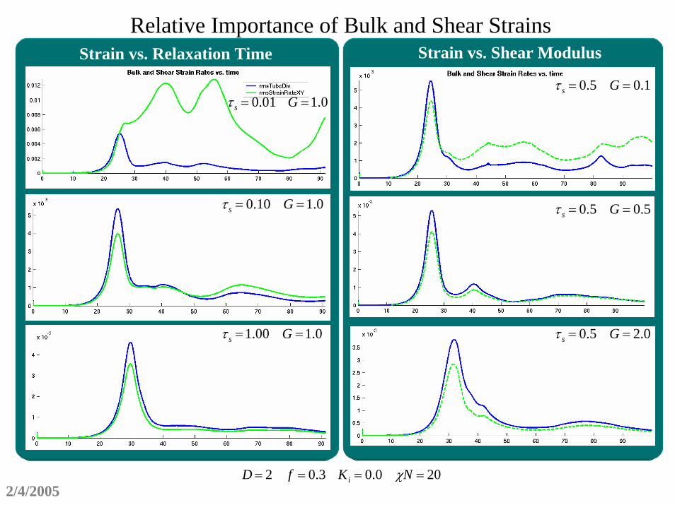
Relative Importance of Bulk and Shear Strains

τ s = 0.01 G =1.0

τ s = 0.10 G =1.0

τ s =1.00 G =1.0

τ s = 0.5 G = 0.1

τ s = 0.5 G = 0.5

τ s = 0.5 G = 2.0

Strain vs. Relaxation Time Strain vs. Shear Modulus

D = 2 f = 0.3 Ki = 0.0 χN = 202/4/2005