kinematic modeling, identification, and control of robotic …
TRANSCRIPT

KINEMATIC MODELING, IDENTIFICATION, AND
CONTROL OF ROBOTIC MANIPULATORS

THE KLUWER INTERNATIONAL SERIES IN ENGINEERING AND COMPUTER SCIENCE
ROBOTICS: VISION, MANIPULATION AND SENSORS
Consulting Editor
Takeo Kanade
Other books in the series:
Robotic Grasping and Fine Manipulation, M. Cutkosky ISBN 0-89838-200-9
Shadows and Silhouettes in Computer Vision, S. Shafer ISBN 0-89838-167-3
Perceptual Organization and Visual Recognition, D. Lowe ISBN 0-89838-172-X
Three Dimensional Machine Vision, T. Kanade ISBN 0-89838-188-6
Robotic Object Recognition Using Vision and Touch, P. Allen ISBN 0-89838-245-9

KINEMATIC MODELING, IDENTIFICATION, AND
CONTROL OF ROBOTIC MANIPULATORS
Henry W. Stone
Carnegie-Mellon University
~
" KLUWER ACADEMIC PUBLISHERS
Boston/Dordrecht/Lancaster

Distributors for North America: Kluwer Academic Publishers 101 Philip Drive Assinippi Park Norwell, MA 02061, USA
Distributors for the UK and Ireland: Kluwer Academic Publishers MTP Press Limited Falcon House, Queen Square Lancaster LA11RN, UNITED KINGDOM
Distributors outside North America: Kluwer Academic Publishers Group Distribution Centre P.O. Box 322 3300 AH Dordrecht, THE NETHERLANDS
Library of Congress CataIoging-in-Publication Data
Stone, Henry W. Kinematic modeling, identification, and control
of robotic manipulators.
(Kluwer international series in engineering and computer science; SECS 29. Robotics)
Based on the author's dissertation-Carnegie Mellon University, 1986.
Bibliography: p. Includes index. 1. Robotics. 2. Manipulators (Mechanism) I. Title.
II. Series: Kluwer international series in engineering and computer science; SECS 29. III. Series: Kluwer international series in engineering and computer science. Robotics. TH211.S76 1987 629.8'92 87-3122
ISBN-13: 978-1-4612-9193-0 e-ISBN-13: 978-1-4613-1999-3 DOl: 10.1007/978-1-4613-1999-3
Copyright 1987 by Kluwer Academic Publishers Softcover reprint of the hardcover 1st edition 1987 All rights reserved. No part of this publication may be reproduced, stored in a retrieval system, or transmitted in any form or by any means, mechanical, photocopying, recording, or otherwise, without written permission of the publisher, Kluwer Academic Publishers, 101 Philip Drive, Assinippi Park, Norwell, Massachusetts 02061.

TO GRETCHEN

Table of Contents
Preface xvii Acknowledgements xix 1. Introduction 1
1.1. Overview 1 1.2. Motivation 2 1.3. Dissertation Goals and Contributions 4 1.4. Dissertation Outline 5
2. Review of Robot Kinematics, Identification, and Con- 7 trol
2.1. Overview 7 2.2. Coordinate Frame Kinematic Models 7
2.2.1. Denavit-Hartenberg Model 10 2.2.2. Whitney-Lozinski Model 15
2.3. Models of Revolute Joint Manipulators 17 2.4. Modeling Assumptions 19 2.5. Kinematic Identification 21 2.6. Kinematic Control 25 2.7. Conclusions 28
3. Formulation of the S-Model 31 3.1. Overview 31 3.2. S-Model 31 3.3. Computing S-Model Parameters 38 3.4. Conclusions 41
4. Kinematic Identification 43 4.1. Overview 43 4.2. Kinematic Features 44

viii TABLE OF CONTENTS
4.3. S-Model Identification 4.3.1. Overview
4.3.1.1. Feature Identification 4.3.1.2. Link Coordinate Frame Specification 4.3.1.3. S-Model Parameter Computation 4.3.1.4. Denavit-Hartenberg Parameter Extraction
4.3.2. Feature Identification 4.3.2.1. Plane-of-Rotation Estimation 4.3.2.2. Center-of-Rotation Estimation 4.3.2.3. Line-of-Translation Estimation
4.3.3. Link Coordinate Frame Specification 4.3.4. S-Model Parameters 4.3.5. Denavit-Hartenberg Parameters
4.4. Conclusions 5. Inverse Kinematics
5.1. Overview 5.2. Newton-Raphson Algorithm 5.3. Jacobi Iterative Method 5.4. Performance Evaluation 5.5. Comparative Computational Complexity 5.6. Conclusions
6. Prototype System and Performance Evaluation 6.1. Overview 6.2. System Overview 6.3. Sensor System
6.3.1. Description 6.4. Generating Features 6.5. Measuring Performance
6.5.1. One-Dimensional Grid 6.5.2. Two-Dimensional Grid 6.5.3. Three-Dimensional Grid
6.6. Kinematic Performance Evaluation 6.6.1. One-Dimensional Performance Evaluation 6.6.2. Two-Dimensional Performance Evaluation 6.6.3. Three-Dimensional Performance Evaluation
6.7. Conclusions 7. Performance Evaluation Based Upon Simulation
45 45 46 46 46 47 47 49 59 65 67 70 71 78 79 79 80 83 87 90 94
97 97 98
101 102 106 111 112 115 117 120 132 135 138 141 145

TABLE OF CONTENTS
7.1. Overview 7.2. A Monte-Carlo Simulator
7.2.1. Evaluating Kinematic Performance 7.2.2. Design Model Control 7.2.3. Signature-Based Control
7.3. Simulator Verification 7.4. Results
7.4.1. Encoder Calibration Errors 7.4.2. Machining and Assembly Errors 7.4.3. Sensor Measurement Errors 7.4.4. Number of Measurements 7.4.5. Effect of Target Radius
7.5. Conclusions 8. Summary and Conclusions
8.1. Introduction 8.2. Summary and Contributions 8.3. Suggestions for Future Research
Appendix A. Primitive Transformations Appendix B. Ideal Kinematics of the Puma 560
B.l. Forward Kinematics B.2. Inverse Kinematics
Appendix C. Inverse Kinematics C.l. Newton-Raphson Computations C.2. Jacobi Iterative Computations
Appendix D. Identified Arm Signtaures Appendix E. Sensor Calibration
E.l. Calibration Rods E.2. Slant Range Compensation
Appendix F. Simulator Components F.l. Robot Manufacturing Error Model F.2. Simulator Input Parameters
Appendix G. Simulation Results G.l. Encoder Calibration Errors G.2. Machining and Assembly Errors
ix
145 147 147 150 154 157 160 160 163 165 167 169 171 175 175 175 180
183 185 185 186 189 189 190 191 193 193 194 199 199 201
205 205 208

x
C.3. Sensor Measurement Errors CA. Number of Measurements C.S. Target Radius
REFERENCES Index
TABLE OF CONTENTS
211 213 216 219 223

List of Figures
Figure 2-1: Two Arbitrary Cartesian Coordinate Frames 9 Figure 2-2: Denavit-Hartenberg Parameters for a Revolute 12
Joint. Figure 2-3: Denavit-Hartenberg Parameters for a Prismatic 13
Joint. Figure 3-1: S-Model Parameters for a Revolute Joint 3"4 Figure 3-2: S-Model Parameters for a Prismatic Joint 35 Figure 4-1: Indexing Joint i to Generate a Plane-of-Rotation 51
and a Center-of-Rotation Figure 4-2: Initial Approximation to the Plane-of-Rotation 57
Using Three Mutually Distant Target Measurements
Figure 4-3: Flow Chart of the Repeated Linear Least- 60 Squares Algorithm for Estimating the Plane-ofRotation
Figure 4-4: Flow Chart of the Repeated Linear Least- 64 Squares Algorithm for Estimating the Centerof-Rotation
Figure 4-5: Coordinate Frame Construction for a Revolute 68 Joint
Figure 4-6: Coordinate Frame Construction for a Prismatic 69 Joint
Figure 5-1: Physical Interpretation of the Jacobi Iterative 85 Algorithm
Figure 6-1: Hardware Configuration 99 Figure 6-2: Arm Signature Identification System and Puma 100
560 Robot. Figure 6-3: GP-8-3D Sonic Digitizer Components 102

xii LIST OF FIGURES
Figure 6-4: Sensor Configuration and Orientation 104 Figure 6-5: Fixture for Attaching Target Point 6 to Link 6 107 Figure 6-6: Approximate Signature Configuration for the 108
Puma 560 Figure 6-7: Flow Chart of the Algorithm for Collecting Tar- 110
get Point Measurements Figure 6-8: Measuring the Performance of a Puma 560 with 113
a Catheto- meter Figure 6-9: Spring-Loaded Pen Assembly Attached to the 116
Puma 560's End-Effector Figure 6-10: Ranky Sensor Jig for Measuring End-Effector 118
Position and Orientation Figure 6-11: Residuals: Normal to Plane and Radial Ooint 123
6) Figure 6-12: Histogram Plots of the Residuals for the Plane- 124
of-Rotation Estimates for Joints 1 through 6 Figure 6-13: Histogram Plots of the Residuals for the 125
Circ1e-of-Rotation Estimates for Joints 1 through 6
Figure 6-14: An Identified Plane-of-Rotation 126 Figure 6-15: Approximate Location of Lines 1 thrmo\1h 6 133 Figure 6-16: Relative Location of Two-Dimensional Grid 136 Figure 7-1: Definition and Location of Points in the Simu- 148,
lated Three- Dimensional Grid Touching Task Figure 7-2: Location of Physical Base Coordinate Frame of 153
the Puma 560 as Defined by the Kinematic Simulator Model without Manufacturing Errors
Figure 7-3: Simulated and Experimental Performance as a 159 Function of Errors in W A,C '(a) X Axis Line (b) Y Axis Line (c) Z Axis Line
Figure 7-4: Radial Position Error Standard Deviations as a 161 function of ae
Figure 7-5: Radial Position Error Standard Deviation as a 164 Function of 0p and 00'
Figure 7-6: Radial Position Error Standard Deviation as a 166 Function of the Measurement Noise Factor k
LIST OF FIGURES xiii
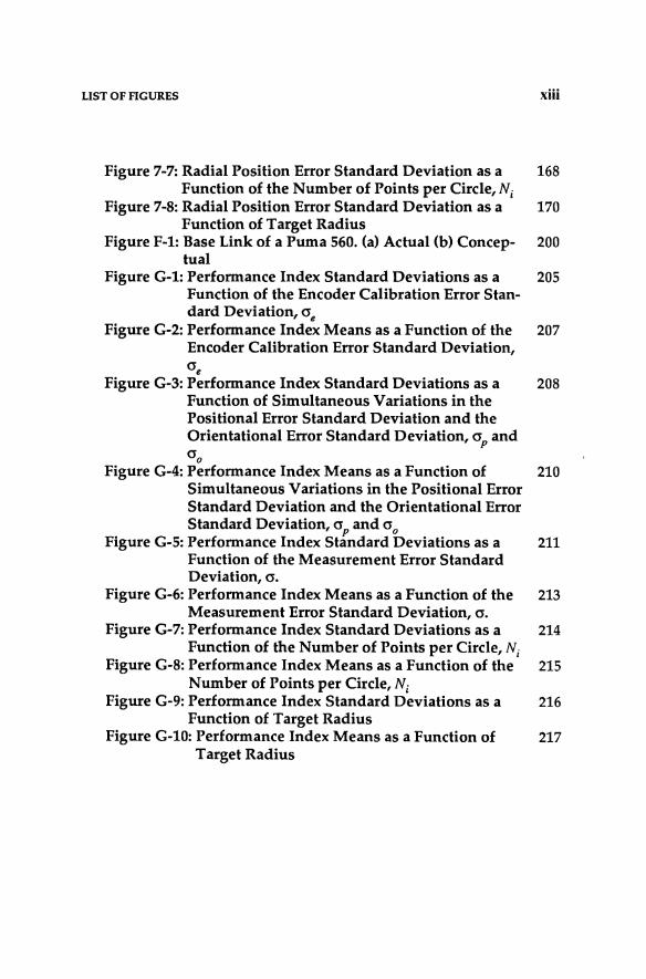
Figure 7-7: Radial Position Error Standard Deviation as a 168 Function of the Number of Points per Circle, Nj
Figure 7-8: Radial Position Error Standard Deviation as a 170 Function of Target Radius
Figure F-1: Base Link of a Puma 560. (a) Actual (b) Concep- 200 tual
Figure G-1: Performance Index Standard Deviations as a 205 Function of the Encoder Calibration Error Stan-dard Deviation, <Je
Figure G-2: Performance Index Means as a Function of the 207 Encoder Calibration Error Standard Deviation, <Je
Figure G-3: Performance Index Standard Deviations as a 208 Function of Simultaneous Variations in the Positional Error Standard Deviation and the Orientational Error Standard Deviation, <Jp and <Jo
Figure G-4: Performance Index Means as a Function of 210 Simultaneous Variations in the Positional Error Standard Deviation and the Orientational Error Standard Deviation, <Jp and <Jo
Figure G-5: Performance Index Standard Deviations as a 211 Function of the Measurement Error Standard Deviation, <J.
Figure G-6: Performance Index Means as a Function of the 213 Measurement Error Standard Deviation, <J.
Figure G-7: Performance Index Standard Deviations as a 214 Function of the Number of Points per Circle, N j
Figure G-8: Performance Index Means as a Function of the 215 Number of Points per Circle, Nj
Figure G-9: Performance Index Standard Deviations as a 216 Function of Target Radius
Figure G-10: Performance Index Means as a Function of 217 Target Radius

List of Tables
Table 4-1: Target Point Correspondence 52 Table 5-1: Typical Convergence Behavior of the Newton- 89
Raphson Algorithm Table 5-2: Typical Convergence Behavior of the Jacobi 89
Iterative Algorithm Table 5-3: Computational Complexity of the Closed-Form 90
Inverse Kinematic Model of the Puma 560 Robot Table 5-4: Computational Complexity of One Iteration of 91
the Newton- Raphson Algorithm Table 5-5: Computational Complexity of One Iteration of 92
the Jacobi Iterative Algorithm Table 5-6: Execution Times of the Motorola 68020 with a 92
68881 Floating Point Co-Processor (12-MHz Clock)
Table 6-1: Puma 560 Target Point Nominal Radii 107 Table 6-2: Unimate Puma 560 Denavit-Hartenberg 120
Kinematic Parameters Table 6-3: Identified Arm Signature Parameters 121 Table 6-4: Sample Variances and Standard Deviations of 126
the Normal and Radial Residuals Table 6-5: Orientational and Positional Accuracy of the 130
Identified Planes-of-Rotation and Centers-ofRotation Corresponding to the Arm Signature of Robot 1
Table 6-6: Line Length Errors 132 Table 6-7: Line Coordinates Measured Relative to Base 133
Coordinate Frame Table 6-8: Two-Dimensional Grid Touching Task Perfor- 137
mance Summary Using the Design Model

xvi LIST OF TABLES
Table 6-9: Two-Dimensional Grid Touching Task Perfor- 137 mance Summary Using the Signature Model
Table 6-10: Three-Dimensional Grid Touching Task Per- 139 formance Summary for Robot 3
Table 6-11: Three-Dimensional Grid Touching Task Per- 140 formance Summary for Robot 5
Table 7-1: Positions of Three-Dimensional Grid Vertices 149 Table 7-2: Nominal Design Kinematic Parameters for a 152
Puma 560 Table 7-3: Propagation of Identification and Control Errors 155 Table D-1: Identified Arm Signature Parameters 191 Table F-1: Offset Transformation Matrix Parameters 202

Preface
The objective of this dissertation is to advance the state-of-the-art in the
kinematic modeling, identification, and control of robotic manipulators with
rigid links in an effort to improve robot kinematic performance.
The positioning accuracy of commercially-available industrial robotic
manipulators depends upon a kinematic model which describes the robot
geometry in a parametric form. Manufacturing error in the machining and
assembly of manipulators lead to discrepancies between the design
parameters and the physical structure. Improving the kinematic perfor
mance thus requires the identification of the actual kinematic parameters of
each individual robot. The identified kinematic parameters are referred to as
the arm signature.
Existing robot kinematic models, such as the Denavit-Hartenberg
model, are not directly applicable to kinematic parameter identification. In
this dissertation we introduce a new kinematic model, called the 5-Model,
which is applicable to kinematic parameter identification, and use it as the
foundation for our development of a general technique for identifying the
kinematic parameters of any robot with rigid links.
The objective of our 5-Model identification algorithm is to estimate the
S-Model kinematic parameters from a set of mechanical features which are
inherent to the manipulator. Each revolute joint possesses two such features

xviii PREFACE
and each prismatic joint possesses one. These features contain the essential
information to model completely the kinematics of a manipulator. The initial
step of the algorithm involves the explicit identification of the feature
parameters. Each feature is identified in an independent procedure and is
based upon measurements of the three-dimensional Cartesian positions of
target points mounted on each of the links of the manipulator. A relatively
simple and systematic method for collecting these measurements is one of
the practical advantages of our approach. The identified feature parameters
are then used to establish the positions and orientations of Cartesian coor
dinate frames fixed relative to each link of the manipulator in accordance
with the definition of the 5-Model. The parameters of the 5-Model are then
computed from the estimated link coordinate frame locations. Finally, the
Denavit-Hartenberg parameters for the manipulator are extracted from the
identified 5-Model parameters.
We have implemented a complete prototype arm signature identifica
tion system and have applied it to identify the signatures and control the
end-effector of seven Unimation/Westinghouse Puma 560 robots. Evalua
tion of the experimental results has demonstrated consistent and significant
improvements in the kinematic performance of all the robots tested.

Acknowledgements
I would like to express my sincere thanks to Professor Arthur
C. Sanderson, my thesis advisor, for his guidance, encouragement, and
patience during my many years at CMU. His thorough reading and con
structive criticism have greatly improved this work. In addition, I am grate
ful for the financial support which he has made available. I thank Professors
Bruce H. Krogh, Friedrich B. Prinz, and Marc H. Raibert for their reading of
the dissertation and their suggestions which have also contributed to im
proving this work. I thank Dr. Gene Bartel for his assistance in developing
the sensor system and associated hardware utilized in our laboratory experi
ments.
Special thanks go to my colleagues, Lee Weiss, Vassilios Tourassis, and
Pradeep Khosla with whom I have had numerous and informative discus
sions, and general commiseration sessions. I would also like to thank my
office mates of late, Nancy Cornelius and Dave Simon, and Angie and Joel
Ferguson , Bill Birmingham, and Ben Motazed for their support and
friendship.
A very special thanks to my parents whom have given me their love
and encouragement.
Finally, and most importantly, I wish to express my love and apprecia
tion to my wife, Gretchen, for her immeasureable patience, encouragement,
and support. Without her this dissertation would not have been possible.

KINEMATIC MODELING, IDENTIFICATION, AND
CONTROL OF ROBOTIC MANIPULATORS

1.1. Overview
Chapter 1
Introduction
This dissertation describes the development of a general technique for
identifying kinematic parameters of serial link robotic manipulators and for
improving their kinematic performance. The research described here ad
dresses three problems in robot kinematics: modeling, parameter identification,
and control. Accurate robot kinematic models are needed to improve the
positioning and orienting accuracy of commercially available robotic
manipulators. The strong inter-relationships between the parameters of cur
rently formulated kinematic models makes it extremely difficult to apply
and guarantee the convergence of standard parameter estimation techniques
such as least-squares. Thus, kinematic models which simplify the identifica
tion process are needed. Kinematic models of manipulators with revolute
joints are inherently nonlinear and identification algorithms must be capable
of accurately identifying the nonlinear kinematic parameters. Since the iden
tified models will not possess closed-form inverse solutions, new methods
for designing and implementing robot kinematic control algorithms must be
developed, which incorporate the identified kinematic parameters, to im
prove robot kinematic performance.
This introduction discusses the significance of these problems and the
motivation for the research (in Section 1.2), and highlights goals and con
tributions (in Section 1.3). The introduction closes with an outline of the
dissertation (in Section 1.4).

2 INTRODUCTION
1.2. Motivation
Robotic manipulators are articulated open chains of serially connected
links. An n degree-of-freedom (OOF) manipulator has n independent joints
and n+l links. The i th joint connects the i-l th and i th links and has one
degree-of-freedom. The joints can either be prismatic or revolute. Actuation
of a prismatic joint translates the link along the joint axis, while actuation of a
revolute joint rotates the link about the joint axis. The base link, Link 0, is
rigidly attached to a mounting surface and the end-effector, Link n, is free to
move in accordance with the actuation of the n joints. Industrial
manipulators are currently used primarily as positioning devices (e.g., for
pick and place operations). In these applications, accuracy of the Cartesian
position and orientation of the end-effector is the control objective.
The design and implementation of robot manipulators require plan
ning of the desired trajectory, followed by analysis of the kinematic and
dynamic characteristics to develop a control system [1B}. Trajectory planners
operate in one of two modes depending upon whether the robot is
programmed with respect to a coordinate frame or programmed in a move
and-teach scenario. When they are programmed with respect to a coordinate
frame, heuristics are applied to compute temporal sequences of the end
effector's Cartesian position and orientation from high-level task descrip
tions. In a move-and-teach scenario, curve-fitting algorithms are used to
compute a joint space trajectory from a series of manually-recorded robot
configurations. Kinematic control, which is the solution of the inverse
kinematic problem (IKP), computes the set of joint positions from the desired
Cartesian position of the end-effector. Dynamic control computes the control
forces and/or torques, which are required to produce the motion specified
by the joint space trajectories. The performance of robotic manipulators
depends upon all three of these factors. This dissertation focuses upon the
INTRODUCTION 3
kinematic modeling, identification, and control of industrial robotic
manipulators for improved positioning accuracy. The design and analysis of
trajectory planners and dynamic controllers are beyond the scope of this
disserta tion.
Kinematic models are required for the analysis and design of robot
controllers. Kinematic models describe the static relationships between the
joint positions and the Cartesian position and orientation of the end-effector.
These relationships are usually expressed in terms of parametric relations
among joint positions and orientations [5,20,26,32]. Increasing the number
of revolute joints in a manipulator dramatically increases the complexity of
the kinematics. The physical interpretation and systematic structure of the
Denavit-Hartenberg model [5] have led to its widespread use in robot control.
The inverse kinematic problem described above uses the parametric
kinematic model to compute the required joint positions for positioning of
the robot arm.
Conventional robot positioning systems rely on the kinematic model to
predict the end-effector position and orientation when only the joint posi
tions are known. Whereas sensory feedback techniques are more appealing,
the real-time measurement of the end-effector's position and orientation is
impractical. In practice, engineers neglect gear backlash, friction, link com
pliance, encoder resolution, joint wobble, and manufacturing errors in for
mulating a kinematic robot model. Standard practice in robot control is to
use the kinematic parameters specified in the robot manufacturer's design,
rather than the actual kinematic parameters that emerge from the manufac
turing process. This approach simplifies the modeling task and facilitates
the implementation of ideal inverse kinematic algorithms for control. In par
ticular, use of an idealized model leads to a closed-form inverse kinematic
solution. This dissertation describes a method for identifying the kinematic

4 INTRODUCTION
parameters of robotic manipulators, evaluates an implementation of the
method, and considers the overall improvement in end-effector positioning
and orienting accuracy.
In the past, positioning errors introduced by the mismatch between the
actual kinematics and the kinematic model have been overshadowed by
more fundamental inadequacies of robotic systems. Over the past decade,
however, marked improvements have been made in the accuracy, reliability,
and dynamic performance of robots. There now exists a need to develop
kinematic control algorithms to improve robot performance [23]. The fact
that engineers often program robots in a move-and-teach mode, thereby cir
cumventing the kinematic controller, to increase positioning accuracy reaf
firms this realization and provides further motivation for this dissertation.
Interest in the kinematic modeling problem has led to the analysis of
kinematic modeling errors and a number of schemes have been proposed for
their identification [4,8, 13, 14, 15,30,31]. Most of these schemes have not
been implemented and evaluated.
1.3. Dissertation Goals and Contributions
This dissertation describes the development of new kinematic robot
models and kinematic parameter identification algorithms for the design of
controllers to improve robot kinematic performance. These models and al
gorithms have been implemented and evaluated on standard industrial
robots. The effects of manufacturing errors upon robot kinematic behavior
and the design of kinematic control algorithms for industrial robots have
been analyzed using simulation tools and compared with experimental
results.
This dissertation contributes to four areas of robotics:

INTRODUCTION
• Kinematic Modeling used for the analysis and design of robot controllers. Our research in this area has led to the development of a new robot kinematic model, called the S-Model, which is directly applicable to the kinematic parameter identification problem.
• Identification of robot kinematic parameters. Our research in this area has led to the development of a practical kinematic parameter identification algorithm called the S-Model identification algorithm.
• Kinematic Performance Evaluntion for the assessment and specification of robot kinematic accuracy.
• Kinematic Control for the design and evaluation of recursive control algorithms for robotic manipulators.
5
We anticipate that our research will impact both the mechanical design and
manufacture of robots and the implementation of advanced control al
gorithms for industrial manipulators. We have shown that implementation
of our proposed identification and control algorithms can increase robot per
formance and thereby expand the range of robotic applications.
1.4. Dissertation Outline
This dissertation is organized as follows. In Chapter 2, we review
robot kinematics, identification, and control. In Chapter 3, we introduce the
new kinematic model, the S-Model, and derive its relationship to the
Denavit-Hartenberg model. Then, in Chapter 4, we apply the S-Model to
formulate the robot arm signature identification algorithm. In Chapter 5, we
describe two algorithms for solving the inverse kinematic problem and
evaluate both their computational complexity and numerical accuracy. The
software and hardware implementation of the S-Model identification algo
rithm and the subsequent control performance evaluation is presented in
Chapter 6. In Chapter 7 we use Monte-Carlo simulation techniques to
evaluate the statistical performance properties of the S-Model identification

6 INTRODUCTION
algorithm. Chapters 3 through 7, which highlight our research, are the major
contributions of this dissertation. Finally, in Chapter 8, we summarize our
contributions and identify areas for further research.

2.1. Overview
Chapter 2
Review of Robot Kinematics, Identification, and Control
In this chapter, we review the formulation of robot kinematic models
and establish robot kinematic control as a framework for the development of
the dissertation. The fundamental problem in the development of robot
kinematic models is the use of geometric and trigonometric principles to
systematically specify the relative positions and orientations of robot joints.
Approaches to this problem are reviewed in this chapter. Standard terminol
ogy is used throughout the dissertation.
2.2. Coordinate Frame Kinematic Models
Coordinate frame kinematic models are based, conceptually, upon the
assignment of Cartesian coordinate frames fixed relative to each of the links.
The spatial transformation between two consecutive link coordinate frames
is a function of the position of the joint which connects the two links
together. In robotics, the (4x4) homogeneous transformation matrix intro
duced by Denavit and Hartenberg [5] and later adopted by Pieper [201 and
Paul [18] has become the most common approach to describing these spatial
transformations. A general homogeneous transformation matrix has the
form

8 REVIEW OF ROBOT KINEMATICS, IDENTIFICATION, AND CONTROL
r Ox ax
p, 1 ny Oy a y Py
Dz Oz 8z pz
0 0 0 1
(2.1)
or, in terms of its vector components,
[~ where
It =
0 =
"it =
is =
11 "It ~l 0 0
[nx ny nz]T
[ox 0y Oz]T
[ax ay az]T
[Pxpypz]T
,and
(2.2)
(2.3)
(2.4)
(2.5)
(2.6)
Consider the two arbitrary cartesian coordinate frames depicted in
Figure 2-1. If the matrix1 C defines the spatial transformation from coor
dinate frame 1 to coordinate frame 2, then the unit direction vectors it, 0, and
"it specify the orientation of the X, Y, and Z axes of coordinate frame 2 in
terms of coordinate frame 1, respectively. The vector is specifies the position
of the origin of coordinate frame 2 with respect to coordinate frame 1.
The (3x3) orthogonal rotation matrix R(3x3) formed by it, 0, and "it is the
orientational component of (2.1) and is is the translational component of (2.1).
The coordinates of a point P in frame 1, Xl = [Xl YI Zl l]T, expressed in terms
of its coordinates relative to coordinate frame 2, x2 = [l2 h z2 l]T, is
lUppercase boldface letters (e.g., Tj and Sj ) denote (4x4) homogeneous transformation matrices.

REVIEW OF ROBOT KINEMA ncs, IDENTIFICA nON, AND CONTROL
y 1
Frame 1 X
1
Z 2
X 2
Figure 2-1: Two Arbitrary Cartesian Coordinate Frames
Frame 2
9
(2.7)
The homogeneous transformation matrix (2.1) has a variety of mathematical
properties which are used extensively in robotics and are presented in [18].
The transformation between any two cartesian coordinate frames can
always be decomposed into a combination of primitive transformations.
Using Paul's notation, the six primitive transformations are
• Trans(x, 0, 0) - Translate x units along the X axis.
• Trans( O,y, 0) - Translate y units along the Y axis .
• Trans( 0, 0, z) - Translate z units along the Z axis.
• Rot(x, e) - Rotate theta degrees about the X axis.
• Rot(y, 9) - Rotate theta degrees about the Yaxis.
• Rot(z, 9) - Rotate theta degrees about the Z axis.

10 REVIEW OF ROBOT KINEMATICS, IDENTIFICATION, AND CONTROL
Paul's notation will be used throughout this dissertation. The elements of
the primitive transformations are evaluated in Appendix A to indicate their
structure.
2.2.1. Denavit-Hartenberg Model
The Denavit-Hartenberg model [5]
(2.8)
has become the standard robot kinematic model because of its physical inter
pretation, strict definition, and multiplicative structure. In (2.8), the (4x4)
homogeneous transformation matrix Til defines the position and orientation
of a coordinate frame fixed relative to the last link (n th link or end-effector)
of a manipulator with respect to a coordinate frame fixed relative to the base
of the manipulator. Conceptually, the right-hand side of (2.8) describes the
spatial relationships between coordinate frames fixed relative to each of the
manipulator links. The Denavit-Hartenberg link coordinate frames, 'l'l for
;=1, ... ,n , are specified such that the forward transformation matrices Ai are
prescribed by
Ai = Ai(qi) = Rot (z,9i)Trans (0, 0, di)Trans (ai,O,O) (2.9) Rot (x, C1.i ) •
The input parameters to the model (2.8) are the n generalized joint coor
dinates qi' The generalized coordinates are used to represent the joint posi
tions without explicitly specifying the physical nature of the joint (i.e.,
whether revolute or prismatic). Expanding (2.9) yields
2Uppercase script letters (e.g., '1i and Si ) denote the symbolic name of a cartesian coordinate system.
REVIEW OF ROBOT KINEMATICS, IDENTIFICATION, AND CONTROL 11
cosei - sinei cos a; sinei sina;
ai sinei ~ 00,9, 1
sinei cosei cosa; - COSSi sma; Ai 0 sin a; d i
(2.10) cosa;
0 0 0 I
In (2.9), the transformation Aj from coordinate frame '1i-l to coordinate frame
'1i is a function of the four Denavit-Hartenberg parameters, 9j , d j , aj , and a?
An n degree-of-freedom manipulator requires the specification of 4'n
parameters, n of which are the controllable joint positions. Geometrically,
the link length, a j , is the length of the common normal between the joint i
and joint i+l axes. The link twist, Clj , is the angle between the joint i and
joint i+ 1 axes measured in the plane perpendicular to the common normal to
the joint axes. The parameter 9 j is the angle, measured in the plane perpen
dicular to the joint i axis, between the joint axis common normals of the i-l th
and i th link. The fourth parameter, d j , is the linear displacement between
the intersections of the link i-l and i axis common normals with the joint i
axis. Figures 2-2 and 2-3 illustrate the physical definition of these parameters
for both revolute and prismatic joints, respectively.
The characteristics of the Denavit-Hartenberg model are immediate
consequences of the Denavit-Hartenberg convention applied to specify the
link coordinate frames. The Denavit-Hartenberg convention follows from a
geometrical analysis of the spatial relationships between consecutive joint
axes. The Denavit-Hartenberg convention specifies the following link coor
dinate frame assignments:
• The Z axis of coordinate frame '1i-l must be parallel to the joint i axis.
3Lowercase letters (e.g., djand I3j) denote scalar parameters.

12 REVIEW OF ROBOT KINEMATICS, IDENTIFICATION, AND CONTROL
Figure 2-2: Denavit-Hartenberg Parameters for a Revolute Joint. Reprinted with permission [18].
• The origin of coordinate frame 'li-l must lie on the joint i axis at the intersection point of the common normal between the joint i-l and joint i axes, and the joint i axis.
• The X axis of coordinate frame 'li-l must be parallel to the common normal between the joint i-l and joint i axes. The positive direction of the X axis points towards the joint i axis.
• The Y axis of coordinate frame ~-l is defined by the vector cross product of the Z axis unit direction vector with the X axis unit direction vector .
• If the joint i and joint i+ 1 axes intersect, the point of intersection is the origin of the 'li-l coordinate frame.

REVIEW OF ROBOT KINEMATICS, IDENTIFICATION, AND CONTROL 13
Figure 2-3: Denavit-Hartenberg Parameters for a Prismatic Joint. Reprinted with permission [18].
• If the joint i and joint i+ 1 axes are parallel the origin of the coordinate frame, 'Ii-I is chosen so that the joint distance d i+l for the next link is equal to zero.
• The origin of the base link coordinate frame, '1Q ' coincides with the origin of the link 1 coordinate frame '1i. .
• The origin of the last coordinate frame, ~ , coincides with the origin of the next to last coordinate frame ~-l .
These assignments guarantee the functional form of the Denavit-Hartenberg
model in (2.8). By using different conventions to specify the link coordinate

14 REVIEW OF ROBOT KINEMA TICS, IDENTIFICATION, AND CONTROL
frames, alternative kinematic models with the same multiplicative structure
as in (2.8) can be formulated. For robots with rigid links and single degree
of-freedom joints, the model in (2.8) is exact.
For a revolute joint, the generalized coordinate qj is the joint i position aj
and the three parameters, d j , aj, and aj are constants. For a prismatic joint, qj
is the joint i position d j and the three parameters aj , aj, and a j are constants.
In practice, the joint encoders of a manipulator are typically calibrated such
that the encoder outputs match the Denavit-Hartenberg joint positions (i.e.,
aj for a revolute joint and d j for a prismatic joint). Without this calibration,
constant offsets must be introduced to specify the difference between the
joint positions measured by the encoder and the joint positions defined by
the Denavit-Hartenberg model. When all of the joint positions are zero, we
say that the manipulator is in the Denavit-Hartenberg Zero Configuration.
From a modeling point of view, the Denavit-Hartenberg model has at
least one potential disadvantage. It can be demonstrated [15,30] that for
some manipulator geometries the definition of the parameter d j may cause
elements of the Aj matrices to be '~xtremely large and hence ill-conditioned.
We have observed such ill-conditione"a Ai matrices with very large elements
in our identification of real robot kinematic model parameters. This situa
tion can lead to numerical instabilities depending upon the application and
the available numerical precision. The ramifications of potentially ill
conditioned transformation matrices upon the kinematic parameter iden
tification problem are discussed in Chapter 4.
The Denavit-Hartenberg parameters are defined according to a concep
tual model of the kinematics rather than a purely physical model. Thus, the
link coordinate frames 'Ii may be located at a point external to the physical
links of the manipulator. This is often the case for manipulators with near
parallel consecutive joint axes.

REVIEW OF ROBOT KINEMATICS, IDENTIFICATION, AND CONTROL 15
2.2.2. Whitney-Lozinski Model
In formulating an approach to the kinematic identification problem,
Whitney and Lozinski [30] use the model
where
Wj = Wj(qj) = Rot(y,Oj)Trans(O,Yj,Zj)Rot(z,"'j)
Rot(y,Oj)Rot(x,'I'j) ,
(2.11)
(2.12)
to describe the rigid body geometric component of the kinematics4. The final
three transformations in (2.12) constitute a general Roll-Fitch-Yaw (RPY)
rotational transformation. Expanding (2.12) yields
Ox Ox ax Px
Dy Oy ay Py Wi = Dz Oz 8z pz
(2.13)
0 0 0 1
where
nx = cosOjCOS"'jcosOj - sin OJ sin ° , (2.14)
fly = sin "'jCOS OJ , (2.l5)
nz = -sin OJ cos "'jCOS OJ - cos OJ sin OJ • (2.16)
Ox == cos OJ [cos "'j sin OJ sin 'l'j- sin "'j cos 'l'j] + sin OJ [cos OJ sin 'l'j] , (2.17)
0, = sin "'jsin OJ sin 'l'j + cos "'jcos'l'j , (2.18)
Oz = -sin OJ [cos "'jsin OJ sin 'l'j-sin"'jCOS 'l'j] + cos OJ [cos 0jsin'l'j] , (2.19)
4The complete model used by Whitney and Lozinski for identification also contains a non-geometric component.

16 REVIEW OF ROBOT KINEMATICS, IDENTIFICATION, AND CONTROL
ax = cos 9 i [cos CPi sin 0i cos 'Vi + sin CPi sin 'Vi] + sin 9j [cos OJ cos 'V) , (2.20)
ay = sinCPisinOicos'Vi - cosCPisin'Vi , (2.21)
az - - sin 9i [cos CPisin gicoS 'Vi + sin CPi sin 'Vi] + cos 9j [cos gicos 'Vi] , (2.22)
Px = zi sin9i , (2.23)
Py E Yi ,and (2.24)
Pz = Zicos 9j (2.25)
In (2.12), the transformation Wj from coordinate frame '1i-l to coordinate
frame '1i is a function of the six parameters, 9j , Yj' Zj , CPj, 0i' and 'Vi. An n
degree-of-freedom manipulator requires the specification of 6·n parameters,
n of which are the controllable joint positions. In contrast to the Denavit
Hartenberg model which requires four parameters per joint, the model in
(2.11) is a non-minimum realization requiring six parameters per joint.
For a revolute joint, the generalized coordinate qj is the joint i position 9i
and the five parameters, Yi' zi' CPi' 0i' and 'Vi are constants. For a prismatic
joint, qi is the jOint i position Yi and the five parameters 9i , zi ' CPi' 0i ' and 'Vi
are constants. For a prismatic joint, the parameter 9i can be arbitrarily set to
zero. Like (2.8), the model in (2.11) is exact for robots with rigid links and
perfect joints. With two additional parameters for each link transformation
matrix, the model in (2.11) conceptually introduces a greater degree of
flexibility in assigning the locations of the link coordinate frames Wi. This
flexibility is reflected in the rules applied to specify the locations of the link
coordinate frames, '1i:
• The Y axis of the link coordinate frame '1i-l must be parallel to the joint i axis in the direction defined by the positive sense of the rotation or translation of the i th joint.
• The origin of the coordinate frame '1i-l must lie on the joint i axis.

REVIEW OF ROBOT KINEMATICS, IDENTIFICATION, AND CONTROL
• The Z axis of the link coordinate frame 'Ti-l must point in the direction such that the origin of coordinate frame 'Ii lies in the plane formed by the Y and Z axis of coordinate frame 'Ii-I when joint i is in its zero position .
• The origin of coordinate frame ~ lies on the joint n axis.
17
The parameters of the model (2.11) have no real physical significance.
Consequently, the model (2.11) lacks the apparent elegance of the Denavit
Hartenberg model. The expression (2.12) for the link transformation matrix
Wi is considerably more complex than the link transformation matrix Ai in
(2.10).
2.3. Models of Revolute Joint Manipulators
In contrast to coordinate frame kinematic models, the models introduced
for rotary manipulators by Mooring [15], Sugimoto and Duffy [25], and Suh
and Radcliffe [26] find their roots in the theory of screws [2]. These models
possess the same multiplicative structure as in (2.8) and (2.11). The Cartesian
position and orientation of the end-effector with respect to the base coor
dinate frame is specified by the transformation matrix
(2.26)
where the constant matrix t,! is the location of the end-effector when all of
the joint positions are zero. For the model (2.26), the zero configuration can
be associated with any arbitrary physical configuration of the manipulator.
The simplest approach is to let the zero positions of the joints correspond
directly to the physical joint encoder readings. In the literature [15], the
homogeneous transformation matrices Di are called displacement matrices
and are functions of the joint positions

18 REVIEW OF ROBOT KINEMA TICS, IDENTIFICATION, AND CONTROL
(2.27)
A displacement matrix specifies the spatial transformation undergone by a
point when it is rotated about an axis in space. The general form of the
displacement matrix is
u;ve + ce uxuyve - uzse uxuz ve + uyse d14
UxUyve + Uzse U;ve + ce uyuz ve - uxse d24 (2.28) Di uxuzve - uyse uyuzve + uxse u;ve + ce d34
0 0 0 1
where
(2.29)
(2.30)
(2.31)
and djk is the (j,k) element of the displacement matrix D, s( e) = sin e j ,
c(e) =cose j, and V(e) = l-cose j • The matrix D j is parameterized by the
six components, ux' uy , Uz 'Px' Py , and Pz of the vectors Uj and Pi' In (2.26),
the unit direction vector Ui points along the joint i axis of rotation and is
referenced with respect to an arbitrarily located base coordinate frame. The
vector Pi specifies the location of an arbitrary point on the joint i axis with
respect to the base frame. Together the two vectors, ui and Pj , locate the
joint axis in space.

REVIEW OF ROBOT KINEMATICS, IDENTIFICATION, AND CONTROL 19
2.4. Modeling Assumptions
The accuracy of a mathematical model of a manipulator is detennined
by the validity of the assumptions upon which it is fonnulated. These as
sumptions are introduced to insure the tractability of the modeling task. In
practice, however, these assumptions are not always satisfied. For robot
control, the resulting inaccuracies give rise to discrepancies between the
predicted and actual end-effector position. The kinematic models reviewed
in Sections 2.2 and 2.3 are based upon the following seven assumptions:
• Link compliance is negligible (A-I).
• Gear train compliance is negligible (A-2).
• Motor-bearing wobble is negligible (A-3).
• Gear backlash is negligible (A-4).
• Link deformation, due to such environmental effects as temperature variations, is negligible (A-5).
• Encoder resolution is infinite (A-6).
• The kinematic parameters of the actual manipulator are known exactly (A-7).
The difference between the predicted and the actual end-effector posi
tions can be reduced by ensuring the validity of underlying modeling as
sumptions. Reduction of this error is critical to improving the kinematic
performance of robotic manipulators. Two approaches are commonly taken
to reduce manipulator-model mismatch. The model can be expanded to
incorporate previously unmodeled features or the manipulator can be
modified to more closely resemble the desired model. For the kinematic
modeling and control of robots, a combination of these approaches appears
to be reasonable.

20 REVIEW OF ROBOT KINEMATICS, IDENTIFICATION, AND CONTROL
The complexity in modeling link compliance, gear train compliance,
bearing wobble, gear backlash, gear friction, link deformation, and encoder
resolution suggests that to incorporate these features into a kinematic model
would be impractical, if not infeasible. Furthermore, since an extremely
wide range of mechanical components are used in the design of manipulator
drive mechanisms, there is little hope that a general model or set of models
could be developed to adequately describe these effects for an arbitrary
manipulator. Commercially, a case by case analysiS of these effects on each
individual manipulator after it is manufactured would be too costly.
Recent advances in robot actuator and sensor technology and com
posite materials for robotic applications improve the validity of many of
these assumptions. Determination of the actual kinematic parameters is a
different issue. Manufacturing errors introduce errors between the actual
kinematic parameters and the design parameters. Unfortunately for many
industrial robots, economic reality precludes the further reduction of
manufacturing tolerances. It thus becomes essential to expand the kinematic
model to account for these manufacturing errors. We must identify either
the manufacturing errors or the actual kinematic parameters. The identifica
tion algorithm developed in this dissertation employs the latter approach.
The observation that the actual kinematic parameters of a manipulator can
vary significantly from the design parameters due to the presence of
manufacturing errors is the principal motivation for the development of this
dissertation. The dissertation relies on Assumptions (A-I) - (A-6).

REVIEW OF ROBOT KINEMA TICS, IDENTIFICATION, AND CONTROL 21
2.5. Kinematic Identification
The goal of a kinematic identification algorithm is to identify the
parameters of a kinematic model which describe the actual position and
orientation of the end-effector in terms of the measured joint positions, and
which incorporates the geometrical variations in the structure caused by
manufacturing errors. Several identification algorithms have been proposed
in the literature [4, 13, 14, 15,30], but to our knowledge only the algorithm
proposed by Whitney and Lozinski [30] has been actually implemented and
evaluated.
The algorithm developed by Whitney and Lozinski is designed to iden
tify both geometric and nongeometric parameters. The geometric
parameters correspond to the kinematic parameters of a rigid body descrip
tion of the robot while the nongeometric parameters represent compliance,
gear transmission errors, and backlash. The model (2.11), presented in Sec
tion 2.2.2, constitutes their description of the geometrical portion of the com
plete robot model. The mathematical form of the non-geometrical com
ponent is derived separately from experiments performed on the robot. The
non-geometrical model maps measured joint positions into actual joint posi
tions. In the example cited, the gear transmission error for one of the joints is
modeled as a sinusoid. The geometrical and non-geometrical models are
combined to form the complete robot kinematic model.
In this approach, a theodolite is used to measure the position of the
robot's end-effector corresponding to various joint configurations. Ad
ditional parameters are introduced into the robot model in order to relate the
Cartesian position of the end-effector to the angular coordinates of the
theodolite. For instance, the coordinates defining the position and orien
tation of the theodolite, relative to the robot, must be included into the new

22 REVIEW OF ROBOT KINEMATICS, IDENTIFICATION, AND CONTROL
model. The model parameters are estimated by minimizing the cost function
(2.32)
... ... where zi is the vector of measured theodolite angular readings, f (ai • ell) is the
vector of predicted theodolite angular readings, ai is the vector of joint en-...
coder readings, ell is the vector of model parameters, and n is the number of
configurations at which measurements are made. A nonlinear least-squares
numerical search algorithm is applied to minimize (2.32).
The authors have implemented their algorithm and have applied it to
improve the kinematic performance of a Puma 560 robot. Twenty eight
geometric parameters and eight non-geometric parameters were identified
using 60 sets of theodolite readings. It appears, however, that in order for
the numerical search to converge, certain parameters within the original
model had to be set to predefined values. Nevertheless substantial improve
ments in performance were obtained. For instance, in one particular case the
relative positioning error of the end-effector was reduced from 4.8 mm to .3
mm.
The identification algorithm developed by Whitney and Lozinski has
several disadvantages.
• The nonlinear minimization algorithm used to estimate the model parameters is not necessarily guaranteed to converge.
• The process of measuring the position of the end-effector is extremely time-consuming and requires a highly skilled operator.
• Analytic models of the non-geometric errors must be developed for each individual robot.
• There is no mechanism for determining at which joint configurations the end-effector's position should be measured to obtain the best estimates.

REVIEW OF ROBOT KINEMA TICS, IDENTIFICATION, AND CONTROL
• Separate procedures must be used to establish a length standard since a theodolite only measures angular displacements.
23
Further analysis and evaluation will be required to fully assess the
capabilities and limitations of this approach.
Mooring [15] has proposed a method for identifying the kinematic
parameters of a revolute joint manipulator using the model (2.26). The basis
for his algorithm lies in the form of the transformation matrix 0i in (2.28). If
the position of joint i is zero, the transformation matrix 0i becomes the
identity matrix regardless of the values of it or p in (2.28). This property
provides a mechanism to partially decouple the identification problem. If,
with the exception of joint i, the positions of all the joints are zero, then the
matrix Tn will be equal to the matrix 0i'
The first step of the identification procedure is to move all joints to
their zero positions. Then, the positions of three points on the end-effector
must be measured and the position of an arbitrary fourth point computed.
The measured positions are combined to form the matrix of measured posi-
tions,
xI,1 XI,2 xI,3 xI,4
YI,I YI,2 YI,3 YI,4 Xl
Zl,l Zl,2 Zl,3 zl,4 (2.33)
1 1 1
After rotating joint i to another position, the positions of the three pOints on
the gripper again are measured, the position of the fourth point is computed,
and the matrix X2 analogous to (2.33) is formed. The eight measurements
correspond to the positions of the same four physical points on the end
effector and thus

24 REVIEW OF ROBOT KINEMA TICS, IDENTIFICATION, AND CONTROL
(2.34)
Since only joint i has a nonzero position, OJ in (2.34) is equivalent to I for j * i and
(2.35)
The elements of 0; in (2.35) can be applied to solve for the kinematic model
parameters (i.e., the elements of the vectors it and p). The process is then
repeated for each of the remaining joints.
The scheme presented in [15] has neither been implemented nor
evaluated using either simulated data or real data. A variation of this
scheme was tested using simulated data and was shown to identify the
robot's true kinematic parameters within "acceptable limits" in [15].
However, this paper did not discuss whether or not the simulated end
effector measurements were corrupted with measurement noise and/or how
measurement noise effects the accuracy of the identified parameters. Further
analysis is required before a judgement as to its potential for improving the
kinematic performance of robots can be made. The development of a sensor
system which can accurately measure the positions of the three points on the
robot's end-effector over a large volume appears to be a major factor in
determining the feasibility and practicality of this approach.

REVIEW OF ROBOT KINEMATICS, IDENTIFICATION, AND CONTROL 25
2.6. Kinematic Control
The kinematic control problem focuses upon the computation of the
joint positions required to locate the end-effector at a desired Cartesian posi
tion and orientation. Since feedback, which requires the measurement of the
Cartesian position and orientation of the end-effector, is often infeasible, we
must implement open-loop feedforward control. In the design of feedforward
control algorithms for industrial robots, we must address the trade-off be
tween algorithm complexity and controller performance. Since the control
algorithms for robots are derived directly from the forward kinematic model,
their complexity increases as the complexity of the forward kinematic model
increases. Incorporating the effects of manufacturing errors into a kinematic
model will lead to increased robot performance at the expense of controller
complexity.
The design of kinematic control algorithms for industrial robots in
volves:
• Formulation of a kinematic model
• Inversion of the forward kinematic model
• Implementation of the inverse kinematic algorithms.
This straightforward approach leads to a relatively simple control algorithm
provided that the initial kinematic model possesses a simple structure.
Kinematic models with closed-form inverses are defined as simple structures.
The fact that relatively few of the possible manipulator configurations pos
sess a closed-form inverse kinematic model has had a strong influence upon
the mechanical design and kinematic modeling of robotic manipulators. For
instance, basic geometrical features, such as parallel or perpendicular joint
axes, are incorporated into the mechanical design of a robot to guarantee the

26 REVIEW OF ROBOT KINEMATICS, IDENTIFICATION, AND CONTROL
existence of a simply-structured kinematic model. In the design of con
trollers for these robots, it is conveniently assumed that the manipulator has
been manufactured with negligible machining and assembly errors. For high
precision applications, the failure of this assumption often accounts for the
observed end-effector positioning errors.
The most difficult task in the design of kinematic control algorithms
has been the formulation of the inverse model. If the Denavit-Hartenberg
formulation is applied to model the kinematics, the backward multiplication
technique of Paul [18] can be applied to derive the inverse kinematics of
simply-structured manipulators. Paul's backward multiplication technique
has contributed significantly to the widespread appeal of the Denavit
Hartenberg formulation. Consider the model in (2.8) where the elements of
the matrix T /I' the desired position and orientation of the end-effector, are
known. Premultiplying both sides of (2.8) yields
(2.36)
The left-hand side of (2.36) is a function of the unknown joint position qI and
known elements of T /I. (The inverse of the homogeneous transformation
matrix Al can be expressed analytically in closed form.) The objective in
Paul's technique is to symbolically expand both sides of (2.36) and to equate
elements on the left-hand side which involve qI with elements on the right
hand side which are independent of the remaining joint positions. The
resulting set of equations are then solved to determine the joint position qI.
The next step uses the solution qI to evaluate the left-hand side of (2.36)
which thus becomes a matrix of known constants. Similarly, by premul
tiplying (2.36) by the inverse of Az 1 we obtain
(2.37)

REVIEW OF ROBOT KINEMATICS, IDENTIFICATION, AND CONTROL 27
The situation is analogous to that in (2.36). The left-hand side of (2.37) is
now only a function of the unknown position q2 and known constants.
Matrix element equality is then employed to isolate and solve for q2' This
procedure is repeated to sequentially solve for the remaining unknown jOint
positions. For revolute joints, the equations involving qj are trigonometric.
The arc tangent function which has two arguments, the ordinate y, and the
abscissa x should be used to solve for qj as opposed to the arc sine or ilrc
cosine functions. The accuracy of the arc tangent function is uniform over its
full range of definition [18]. Based upon the sign of its arguments, the arc
tangent function returns an angle in the interval-1t to 1t.
The premultiplication procedure described above will require
modification if two or more of the joint axes are parallel. For instance, if the
joints i and i+l are parallel, the sum of the two joint positions qj and qj+i
must first be determined in one step followed by determination of either qi or
qj+1 in the following step. Hence, after solving for qi-I' we expand
(2.38)
-I -I The elements of Aj+I"Aj will be a function of the sum (qj + qj+I)' After
solving for this sum, other elements of (2.38) can be used to solve for the
individual joint positions.
Most manipulators with revolute joints, especially anthropomorphic
manipulators, can reach a desired end-effector location in one of several
distinct joint configurations. The Puma 560, which has six revolute joints,
has, in general, eight distinct solutions. The multiplicity of inverse kinematic
solutions for a given end-effector location can be easily computed using
Paul's technique. However, since the model (2.8) does not account for the
mechanical joint limitations, not all the multiple solutions are physically ach-

28 REVIEW OF ROBOT KINEMATICS, IDENTIFICATION, AND CONTROL
ievable. The ability to reach a particular joint configuration can only be
determined after the solution has been evaluated.
We indicated in Section 2.4 that kinematic models of increasing com
plexity and accuracy are needed to improve robot positioning performance.
Since these models will not have closed-form inverses, numerical algorithms
must be applied to solve the inverse kinematic problem. Application of
these algorithms gives rise to such issues as the rate of convergence, conver
gence to a global versus a local minimum, and the feasibility of real-time
implementation.
2.7. Conclusions
In this chapter, we have reviewed robot kinematic modeling, identifica
tion, and control techniques, and established a framework in which to
present our research contributions.
We introduced the concept of coordinate frame kinematic models (based
upon the conceptual notion of fixing Cartesian coordinate frames to the
various links of a robot). The analytiC properties and physical interpretation
of the Denavit-Hartenberg model which has become widely used in both
industry and academia for modeling robot kinematics were discussed. The
model used by Whitney and Lozinski [30J and the displacement matrix model
used to model the kinematics of revolute joint manipulators were also
presented. We then delineated the engineering assumptions upon which
these models are formulated. We reviewed the kinematic parameter iden
tification algorithms proposed by Whitney and Lozinski [30J and Mooring
[15J, and outlined some of practical problems with each of these approaches.
Finally, we formulated the robot kinematic control problem and reviewed
the Backward Multiplication Technique developed by Paul [18J.

lEVIEW OF ROBOT KINEMATICS, IDENTIFICATION, AND CONTROL
In this dissertation, we:
• Develop (in Chapter 3) a new robot kinematic model, called the S-Model, whose analytic properties and conceptual formulation make it directly amenable to identification.
• Develop (in Chapter 4) the S-Model identification algorithm which can be applied to identify the kinematic parameters of any robotic manipulator with rigid links.
• Synthesize and evaluate (in Chapter 5) two methods for inverting identified arm signature models.
• Develop (in Chapter 6) a prototype arm signature identification system and apply it to significantly improve the performance of several standard robotic manipulators.
• Evaluate and compare Chapter 7 the statistical performance of the design model based and signature-based approach to robot kinematic control.
29

3.1. Overview
Chapter 3
Formulation of the S-Model
In this chapter, we introduce the formulation and properties of a new
kinematic model for describing robot kinematics. This kinematic model,
which we call the S-Model, was designed to facilitate kinematic parameter
identification. This model can be applied to model the kinematics of all
robotic manipulators which satisfy assumptions (A-I) through (A-7) (refer to
Chapter 2).
3.2. S-Model
Like the Denavit-Hartenberg model, the S-Model is a general method
of describing and characterizing kinematics of robotic manipulators. In the
S-Model, the matrix
(3.1)
defines the position and orientation of a coordinate frame fixed relative to
the last link of a manipulator with respect to a coordinate frame fixed rela
tive to the base link. The general transformation matrices, Hi' in (3.1) are (4x4)
homogeneous transformation matrices. The Hi and Sn matrices in (3.1) arc
analogous to the Ai and Tn matrices of the Denavit-Hartenberg model in
(2.8). The symbolic name Si signifies the ith link coordinate frame defined by

32 FORMULATION OF THE S-MODEL
the S-Model. The transformation matrix, Bi , describes the relative transfor
mation between the Si-l and Si coordinate frames (measured with respect to
the Si-l coordinate frame). In the S-Model, six parameters, ~i ' di ' iij , ~ , 'Yj ,
and bi , define the transformation matrix
Bj = Rot(z'~i)Trans(O,O,di)Trans(ii,O,O)Roi(x,o.i)
Rot (z, 'Yi )Trans (0, 0, b i)
Expanding (3.2) yields
nx Ox sin~i sina;. bi sin~i sina;. + 3i COS~i 1 ny Oy - COS~i sin a;. - bi COS~i sina;. + 3i sin~i
sina;. Sin'Yi sina;. C0S"fi cosa;. b, COS~ + ~ j 0 0 0
where
nx - cos ~ i cos 'Yi - sin ~ . cos (X. si,n 'Y. , I I I
ny = sin ~ i cos 'Yi + cos ~.cos(X.sin 'Y' , I I, I
Ox - -cos ~isin 'Yi - sin ~i cos (Xi cos 'Yi ,and
0y - - sin ~i sin 'Yi + cos ~icOS (Xicos'Yi
(3.2)
(3.3)
(3.4)
(3.5)
(3.6)
(3.7)
To specify the S-Model for an n degree-of-freedom manipulator thus re
quires 6'n parameters.
To insure that the manipulator's kinematics can be modeled by (3.1),
we introduce an S-Model convention to define the allowable locations of the
link coordinate frames. Because each link transformation matrix is specified
by six parameters rather than by four, the S-Model convention is less restric
tive than the Denavit-Hartenberg convention.
The following four aSSignments, which are a subset of the Denavit-

FORMULATION OF THE S-MODEL 33
Hartenberg convention reviewed in Section 2.2.1, specify the locations of the
S-Modellink coordinate frames:
• The Z axis of the link coordinate frame, Sj-l ' must be parallel to the joint i axis in the direction defined by the positive sense of the rotation or translation of the i th joint.
• The origin of the coordinate frame, Sj-l ' must lie on the joint i axis.
• The Z axis of the last coordinate frame, Sn' is parallel to the Z axis of the next to the last coordinate frame, Sn-l'
• The origin of the last coordinate frame, Sn ' lies on the joint n-l axis.
There are two fundamental distinctions between the Denavit
Hartenberg link coordinate frames, 'Ii ' and the S-Model link coordinate
frames, Sj. First, in contrast to the origin of 'Ii which is fixed, the location of
the origin of Sj on the joint i+l axis is arbitrary. Second, the direction of the X
axis of Sj must only be orthogonal to the Z axis. The arbitrary location of the
origin of Sj along the joint axis and the arbitrary orientation of the X axis of Si
provide an infinite number of link coordinate frames, So through Sn ' which
satisfy the 5-Model convention.
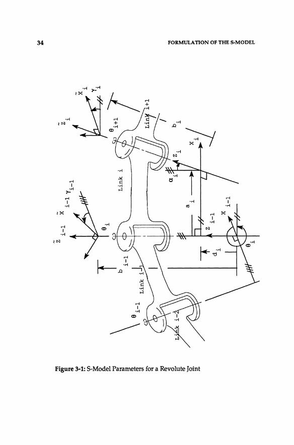
The transformation matrix, Bj , can be formulated from the geometry of
either Figure 3-1 or Figure 3~2. In Figures 3-1 and 3-2, we apply the S-Model
convention to define a pair of link coordinate frames, Sj_l and Sj. For com
parison, we also depict the Denavit-Hartenberg coordinate frames 'Ii-I and 'Ii . The angle Yj is defined as the angular displacement between the X axes of
the Denavit-Hartenberg coordinate frame 'Ii and the S-Model coordinate
frame Sj. The parameter b j is defined as the linear displacement between the
origins of the Denavit-Hartenberg coordinate frame 'Ii and the 5-Model1ink
coordinate frame Sj' If the displacement is in the direction of the Z axis of
joint i, then Yj is positive.
34 FORMULA nON OF THE S·MODEL
Figure 3-1: 5-Model Parameters for a Revolute Joint

FORMULA nON OF THE S-MODEL 35
Figure 3-2: S-Model Parameters for a Prismatic Joint

36 FORMULATION OF THE S·MODEL
The transformation matrix, Bi , specifies the spatial transformation be
tween the Sj_I and Sj link coordinate frames for both prismatic and revolute
joints. From Figure 3-1 and the definitions of 'Yj , b j , and Aj , the transfor
mation matrix, Bj , is the product
Bj = Rot (z'-Yi-I )Trans (0, O,-bH HRot(z, 9j )Trans (0, 0, d j )
Trans (ai' O,O)Rot (x, (Xi) ]Rot(z, 'Y)Trans(O,O, bj) . (3.8)
The first transformation, Rot (z'-Yj_I ), aligns the orientation of the axes of
coordinate frames Sj_I and '1i-I The second transformation,
Trans(O,O,-bi-I)' translates the origin of Sj_I so that it coincides with the
origin of the Denavit-Hartenberg coordinate frame '1i-I . The four bracketed
transformations define the Denavit-Hartenberg matrix Aj • (The parameters
9j , dj , aj , and (Xj are the Denavit-Hartenberg parameters for link i.) These
four transformations transform coordinate frame 'Ii-I to the Denavit
Hartenberg coordinate frame '1i. In analogy with the first two transfor
mations, the cascade Rot (z, Yj )Trans (0, 0, b j) transforms the Denavit
Hartenberg coordinate frame '1i to the S-Modellink coordinate frame Sj •
By combining terms according to the rules of homogeneous transfor
mations [18], Bj in (3.8) simplifies to
Bi = Rot(z,9i-Yi_l)Trans(0,O,di-bi_l)Trans(ai'0,0)
Rot (X, (Xj)Rot (z,-Yj)Trans(O, 0, b)
Since (3.2) and (3.8) are equivalent,
R. = 9· - '11. 1 1-'1 I '1-
d. = d. - b· I ' I I 1-
(3.9)
(3.10)
(3.11)
where the joint rotational offset, Yi' and the joint translational offset, b j , are
constant parameters.

FORMULATION OF THE S·MODEL 37
If joint i is revolute, ~j is a function of the joint position OJ and the
remaining five parameters, dj , i j , ~ , Yj , and bj , are constants. If joint i is
prismatic, dj is a function of the joint position dj and the remaining five
parameters, ~j , i j , a; , Yi' and b i ' are constants. For a manipulator with
revolute joints, the four Denavit-Hartenberg parameters are extracted from
the six 5-Model parameters according to
(3.12)
(3.13)
(3.14)
(3.15)
According to the Denavit-Hartenberg model, the link transformation
matrix
Aj = Aj(qj) == Rot(z,Oj)Trans(O,O,dj)Rot(x,exj ) , (3.16)
for a prismatic joint and the parameter aj , is by definition zero. This con
dition is guaranteed by requiring that the axis of the prismatic joint, joint i,
be chosen to intersect with the joint i+l axis, as illustrated in Figure 2-3.
Thus, the location of the coordinate frame '1f-l is constrained even more for a
prismatic joint than for a revolute joint. This is not the case in the 5-Model.
From Figure 3-2, it is, in general, impossible to model the spatial transfor
mation between the 5j- 1 and 5j link coordinate frames by the general trans
formation matrix in (3.2) with the parameter i j set to zero. Thus, if we were
to apply the relations (3.12) - (3.15), the computed Denavit-Hartenberg
parameter aj would be nonzero. The parameters OJ, d j , aj , and exj obtained
in this way for a prismatic joint are called the modified Denavit-Hartenberg
parameters. In the modified model, the origin of the coordinate frame '1i-l is

38 FORMULATION OF THE 5-MODEL
arbitrary. In Chapter 4, we present a method for determining the true
Denavit-Hartenberg parameters for manipulators with prismatic joints.
3.3. Computing S-Model Parameters
In this section, we apply the backward multiplication technique [18] to
derive the closed-form expressions for the 5-Model parameters, ~i ' di ' ai '
n;, 'Yi' and b i , in terms of the elements of the general transformation matrix
Bi ·
The transformation matrix Bi is given by
o ~
o
Px 1 Py
pz 1
(3.17)
where the individual elements are known. Premultiplying (3.2) by
ROll (z, ~i) yields
Rot-l (z'~i)'Bi = Trans(O,O,di)Trans(ii,O,O)Rot(x,n;)
Rot(z, 'Yi)Trans(O,O, b i ) , (3.18)
which when expanded becomes
COS~i Sin~i 0 0
- sin~i cos~ 0 0
0 0 1 0 Bi
0 0 0 1

FORMULATION OF THE S·MODEL 39
COSYi - SinYi 0 8i
COSa; sinYi cosa; COSYi - sina; - bi sina;
sina; SinYi sinYi cosa; bi cosa;. + di (3.19)
0 0 0 1
An expression for ~i is obtained by equating the (1,3) elements in (3.19)
(3.20)
From (3.20), we obtain the two solutions
-a ~i = atan-" and
ay (3.21)
~i = ax
atan- . -ay (3.22)
which differ by 180 degrees. If both ax and ay are zero, the i th and i+ 1 th joint
axes are parallel and the parameters ~i and Yi are redundant. When this
situation occurs, we can arbitrarily set ~i to zero. Thus,
~i = 0 (3.23)
when ax=ay=O. The rotational parameter ii; can be expressed in terms of Pi by equating the (2,3) and (3,3) elements in (3.19). The expressions are
(3.24)
(3.25)
Having computed Pi using either (3.21) or (3.22), the unique solution for ~
obtained from (3.24) and (3.25), is

40 FORMULATION OF THE S-MODEL
(3.26)
Two expressions involving 1i and ~i can also be obtained from (3.19). Equat
ing the (1,1) and (1,2) elements in (3.19) yields
(3.27)
(3.28)
Using (3.27), (3.28), and ~i ' the unique solution for 1i is
(3.29)
The solution for i\ is obtained by equating the (1,4) elements in (3.19). Thus,
Equating the (2,4) elements in (3.19) yields
from which we obtain the solution
__ -P.xsin~i + PyCOS~i bi
sinai
bj = 0
(3.30)
(3.31)
if sinaj=O . (3.32)
Finally, equating the (3,4) elements in (3.19) and rearranging, yields the solu
tion for (Ii ' namely
(3.33)

FORMULATION OF TIlE S-MODEL 41
In chapter 4, we apply the solutions (3.21), (3.26), (3.29), (3.30), (3.32),
and (3.33) in formulating the S-Model identification algorithm.
3.4. Conclusions
The S-Model described in this chapter offers several advantages for the
development of a kinematic identification algorithm:
• The flexibility in assigning link coordinate frames leads to a simple, efficient, and accurate algorithm for identifying the location of the S-Modellink coordinate frames Sj for i =<>, ... ,n-l
• The Denavit-Hartenberg model parameters may be extracted from the S-Model parameters according to (3.12) - (3.15)
The development of a kinematic identification algorithm using these prin
ciples is described in the next chapter.

4.1. Overview
Chapter 4
Kinematic Identification
The goal of a kinematic identification algorithm is to identify the
parameters of a kinematic model which describes the actual position and
orientation of the end-effector in terms of the measured joint positions, and
which incorporates the geometrical variations in the structure caused by
manufacturing errors. Either the Denavit-Hartenberg model or the S-Model
are adequate to provide an exact description of the actual robot kinematics.
Identification of these parametric models, however, requires detailed con
sideration of the structure of the models as well as an adequate procedure to
measure robot configurations. Because of manufacturing errors, all exact
kinematic models will possess non-simple structures leading to more com
plex control algorithm design and implementation tasks.
While the Denavit-Hartenberg model is specified by a minimum num
ber of parameters, it possesses a rigid structure and is not amenable to direct
identification. The term "rigid" signifies that all the parameters and com
ponents to the model are precisely defined and are unique. In contrast, the
S-Model is directly applicable to kinematic identification. The relationships
in (3.12) - (3.15) provide a mechanism for calculating the Denavit-Hartenberg
parameters from the identified S-Model parameters.
In Section 4.2, we describe the intrinsic properties of mechanical joints,

44 KINEMATIC IDENTIFICATION
referred to as the kinematic features. Then, in Section 4.3, we develop the
S-Model identification algorithm.
4.2. Kinematic Features
The objective of S-Model Identification is to estimate the S-Model
kinematic parameters from a set of 2nr+np mechanical features inherent to
the manipulator, where nr is the number of revolute joints and np is the
number of prismatic joints. (The number of degrees-of-freedom n=nr+np ).
The two features of a revolute joint are called the center-of-rotation and the
plane-of-rotation, and the feature of a prismatic joint is called the
line-of-translation.
These features are derived from basic geometric considerations of the
joints. The locus of a point rotating about an axis is a circle lying in a plane,
called the plane-of-rotation and the normal to this plane is a vector which is
parallel to the axis of rotation. The center of the circle is a point, called the
center-of-rotation which lies on the axis of rotation. When joint i-1 of a
manipulator is rotated, any point which is fixed relative to the i th link
defines a plane-of-rotation and a center-of-rotation, under the assumption
that the positions of joints 1 through i-2 remain fixed. We associate this
plane-of-rotation and center-of-rotation with the (i-1) th joint and the i th link.
The line-of-translation is a feature of a prismatic joint. When a point is
displaced linearly, its trajectory is a straight line which is parallel to the
vector which indicates the direction of the displacement. For a manipulator,
any point which is fixed relative to link i defines a line-of-translation when
joint i-I is moved, under the assumption that the positions of joints 1 through
i-2 remain fixed.

KINEMATIC IDENTIFICATION 45
4.3. S-Model Identification
4.3.1. Overview
The approaches to solving the manipulator kinematic parameter iden
tification problem discussed in Chapter 2 all propose to identify the
kinematic parameters directly and explicitly from a set of observed measure
ments, typically the position and/or orientation of the end-effector. Since
the kinematics of any manipulator with at least one revolute joint will be
nonlinear, such a direct method inevitably leads to a nonlinear minimization
problem. In contrast, the S-Model identification algorithm is an indirect
method of identification which leads naturally to a separation of the iden
tification problem into a set of independent, less complex minimization
problems.
In this section, we describe our solution to the kinematic parameter
identification problem. The detailed formulation and implementation are
presented in subsequent sections. The 5-Model identification algorithm in
cludes four steps:
1. Feature identification
2. Link coordinate frame specification
3. S-Model parameter computation
4. Denavit-Hartenberg parameter extraction

46 KINEMATIC IDENTIFICATION
4.3.1.1. Feature Identification
In the first step, feature identification the kinematic features are iden
tified from measurements of the Cartesian position of targets physically at
tached to the robots links. The positions of these targets, relative to an
independent fixed coordinate frame, vary as the manipulator changes its
configuration. During data collection the manipulator is programmed to
move through a sequence of jOint configurations. At each configuration the
position of a target is measured. The kinematic features are described
analytically by an algebraic equation, and the coefficients of these equations
are the feature parameters which are estimated.
4.3.1.2. Link Coordinate Frame Specification
The second step in our identification algorithm is link coordinate frame
specification. If the manipulator configuration is known in terms of the joint
positions a set of link coordinate frames which satisfy the S-Model conven
tion (in Section 3.2) may be defined. By collecting target measurements and
identifying the parameters of the kinematic features which correspond to
this same manipulator configuration, we can readily establish a valid set of
S-Modellink coordinate frames. Then, we can apply the estimated feature
parameters to construct and evaluate the elements of the matrices Sj in (3.1).
4.3.1.3. S-Model Parameter Computation
The third step, S-Model parameter computation applies the application of
the inverse kinematic parameter relationships developed in Section 3.3. The
elements of the general transformation matrices Bj , which are the arguments
to these inverse relationships, are a function of the transformation matrices Sj
determined in the previous step. Identifying the S-Model parameters re
quires straightforward numerical evaluation.

KINEMATIC IDENTIFICATION 47
4.3.1.4. Denavit-Hartenberg Parameter Extraction
In the fourth and final step, Denavit-Hartenberg parameter extraction the
relationships developed in Section 3.2 are applied to determine the
manipulators Denavit-Hartenberg kinematic parameters from the identified
S-Model parameters.
The procedure for varying the configuration of the manipulator in or
der to obtain the necessary measurements of the target positions and the
analytic techniques for solving for the estimated feature parameters are
presented in Section 4.3.2. In Section 4.3.3, we introduce the rules for es
tablishing valid S-Model link coordinate frames and constructing the
matrices Sj. Evaluation of the general transformation matrices and the S
Model parameters are described in Section 4.3.4 with special attention given
to the determination of the first and last link parameters. Finally, in Section
4.3.5, we review the procedure for extracting the Denavit-Hartenberg
parameters and introduce the notion of a pseudo Denavit-Hartenberg model
to account for physical alignment constraints.
4.3.2. Feature Identification
Identifying a plane-of-rotation and a center-of-rotation is conceptually
straightforward. Imagine an arbitrary target point fixed relative to link i+1.
When joint i is rotated, this target point traces a circle in space. The plane in
which the circle lies is, by definition, a plane-of-rotation. The coeffic~ents of
the equation of this plane can be estimated from a curve fit of m measured
Cartesian positions of the target along the circle corresponding to m different
positions of joint i. (It is assumed that all Cartesian measurements are made
with respect to the sensor frame). The center of the traced circle, defined by
its thr~imensional Cartesian coordinates, is the center-of-rotation. We can

48 KINEMATIC IDENTIFICATION
extract the coordinates of the center-of-rotation from an estimate of the
parameters of the equation for the traced circle. Identifying a line-of
translation is also straightforward. When joint i is translated, the target point
traces a line in space. The parameters of the line, which constitute the
line-of-translation, can be estimated by fitting the measured target locations to
the equation of a line.
In practice, the target point may be a physical location on the i+l st link
or a location of a point on a body which is attached rigidly to link i+l. We
will refer to the target point attached to link i+l as the i th target point or as
target point i. The flexibility in choosing the location of the target point is
another important advantage of our approach. For a revolute joint, the
nominal radius of the target point to the jOint axis can be controlled to ac
commodate the sensor system constraints and to enhance feature estimate
accuracy. We will return to the issue of enhancing estimate accuracy once
we have formulated and presented solutions to the feature parameter es
timation problem.
Identifying a plane-of-rotation and a center-of-rotation from a set of
points in three dimensions corresponds to the problem of fitting such points
to a circle. In this problem, the parameters to be identified are the coor
dinates of the center of the circle, the circle's radius, the unit normal vector to
the plane in which the circle lies, and the coordinates of n points lying on the
circle corresponding to each of the n measured points. Given the measured
positions of the target points, PI ' P2' ... 'Pn we wish to minimize the
function
(4.1)
subject to the constraints

KINEMATIC IDENTIFICATION 49
IIXj - jJlj2 - ,2 = 0 , (4.2)
(4.3)
11011 - 1 = 0 , (4.4)
and minimized with respect to the 3·n + 7 scalar parameters contained within
p, a, r, Xl' XZ , ••• ,X". The vector p defines the Cartesian position of the
center of the circle, the vector a defines the unit vector normal to the plane in
which the circle lies, r is the radius of the circle, and the vectors xi for i= 1,2, ... ,n define the Cartesian position of n points on the circle. This
constrained minimization problem can be transfonned into an equivalent
unconstrained minimization problem using LaGrange's technique. The solu
tion is then given by the solution to a set of 5·n + 8 simultaneous nonlinear
algebraic equations in the same number of unknowns. The additional 2·n + 1
unknowns are LaGrange multipliers. In practice, the minimization of (4.1)
becomes an extremely difficult problem to solve when the number of
measurements, as in our implementation, is on the order of 50 to 100. In
Sections 4.3.2.1 and 4.3.2.2, the problem of identifying the plane-of-rotation
and center-of-rotation is separated into two independent problems. The
combination of the two solutions is both realistically and intuitively pleasing.
4.3.2.1. Plane-of-Rotation Estimation
We present two methods for fitting the measured target positions of a
revolute joint to a plane. Our objective is to minimize the sum of the perpen
dicular distances between the measurements and the estimated plane. The
solution to this minimization problem yields the coefficients which define an
estimated plane-of-rotation. The first method [1], is based on an error
measure divided by its average gradient and uses an eigenvalue solution.
The second method approximates the solution of the desired minimization

50 KINEMATIC IDENTIFICATION
problem by the repeated application of a linear least-squares regression. In
formulating the latter, we rely heavily upon our a priori knowledge of and
control over the generation of the target positions. We have incorporated
both algorithms into our 5-Model identification algorithm. In Chapter 6 we
demonstrate experimentally that for measurements obtained using an
ultrasonic sensor system, the performance of these two algorithms is iden
tical (Le., the same feature parameters are obtained). For sensor systems
with different noise properties and/or physical constraints upon the
measurable target locations, the two algorithms may yield differences in per
formance. The linear least-squares solution is easier to implement in
software. The eigenvalue solution is analytically exact.
While measuring the poSition of the ; th target, joints 1 through ;-1 are
required to be in their corresponding signature configuration positions.
Joints ;+1 to n, on the other hand, can be positioned arbitrarily. Through
independent control of the manipulators joints, joint i is then sequentially
indexed to m different positions, qi,j for j = I, ... ,m. These positions should
be uniformly spaced about the physical range of motion of joint i. To later
maintain a correct sense of rotation, it is assumed that the positions qi,j are
ordered such that qi,j < qi,j+l' as illustrated in Figure 4-1. Thus, the interval
between successive joint positions
(4.5)
where q~ and q~ are the corresponding minimum and maximum limits
for joint i, respectively. At each successive configuration, the Cartesian posi
tion of the i th target, denoted by the column vector Pj=[xj'Yj,Zj]T , is
measured with respect to the sensor frame. The correspondence between the
manipulator configurations and the target position measurements is listed in
Table 4-1.

KINEMATIC IDENTIFICATION
• P ,p • 4 ' 3 '. i, , ;/P 2 ~ . ,
\ . , \ , I I \ , , , \ , . ' ~ ......... ~----:--- ... ..,,/
", \ \ : ,' ......... ", \ ~ : " ... , \ I , , , \ , , ,
, \ , , I " \ ~ : " , \ I , " e P.: \~:,' max J: \" ---1t-----li--------------~--------------------
I ,I' , II \ , , I \ , , , \
\ : \ \ \" : \ \
'......... ; \ '\ Joint Axis
51
....... , \ " ··.-L ___ ~_--- .. \ Out of Page , . \ , . \
: \ " ~ ~--'!. , • P
• m-l
Figure 4-1: Indexing Joint i to Generate a Plane-of-Rotation and a Center-of-Rotation
The normal form for the equation of plane is
Ax + By + Cz + D = 0 , (4.6)
where the coefficients A, B, C, and D are the parameters to be identified. We
chose as the measure of error between the measured target position and the
plane the function
~(x,y,z) = Ax + By + Cz + D
~(x,y,z) q,Te = eTc!> (4.7)

52 KINEMATIC IDENTIFICATION
Table 4-1: Target Point Correspondence
Manipulator Configuration Measured Target Position
Pl =[xl Yl zl ]T
P2=[.xz Yz z2]T
• • • • • •
p.= [x· y. J J J
z.]T J
• • • • • •
pn=[xn Yn z ]T n
where
<P = [x y z l]T , (4.8)
and
e = [A B C D]T (4.9)
are the augmented information vector and parameter vector, respectively.
At a point on the plane, the error function ~(x,y,z) is zero. It is also observed
that the magnitude of the error function increases at points farther away
from the plane. For points close to the plane, the error function is propor
tional to the perpendicular distance from the point to the plane. The con
stant of proportionality is the reciprocal of the magnitude of the gradient of
~(x,Y, z). The magnitude of the error is

KINEMATIC IDENTIFICATION
Using the m measured target positions, Pi,i' the aggregate error is
where
m
4> = I,(CIHlh . 1 J J r-
53
(4.10)
(4.11)
(4.12)
Minimizing the sum of the squares of the perpendicular distances between
the measured target points and the plane is equivalent to minimizing :::
under the constraint that the average magnitude of the gradient of the error
function at the measured target points, Pi,i' for j= 1, ... ,m, is unity. The
squared magnitude of the gradient of the error is
(V~)2 == (a~)2 + (~}2 + (a~)2 = aT'P9 ax ay az (4.13)
where 'P is the (4x4) diagonal matrix Diag [1 1 1 0]. Since 'P is constant, the
constraint requiring that the. mean-squared gradient of ~ equal unity is
equivalent to setting (4.13) equal to one,
9 T'P9 = 1 . (4.14)
We thus seek the parameter vector 9 that minimizes (4.11) subject to the
constraint (4.14). Using LaGrange multipliers, the solution to this con
strained minimization is given by the solution to the generalized eigenvalue
problem [24]
4>9 = A'P9 , (4.15)
where A is a scalar. Using (4.11) and (4.15), the aggregate error :::=Am.

54 KINEMATIC IDENTIFICATION
Therefore, the desired set of parameters are given by the eigenvector cor
responding to the smallest eigenvalue. The singularity of 'II precludes the
direct application of typical eigenvalue methods to solve (4.15). To solve
(4.15), we first partition it into the form
LX·2 J LXjYj L XjZj LXj A
LYjXj LY[ L YjZj LYj B
L ZjXj L ZjYj L z·2 l LZj C
LXj LYj L Zj m D
1 0 0 0 A
0 1 0 0 B
A- 0 0 1 0 C (4.16)
0 0 0 0 D
where summations from j = 1 to m are indicated by the symbol L. The scalar
equation defined by the bottom row in (4.16) yields the solution for the
parameter D, namely,
m m m
D = A L Xj + B L Yj + C L z·
j=l j=l j=l )
m (4.17)
= - (Ai + By + Cz)
where X, y, and z are the sample means of the x, y, and z coordinates,
respectively. Substituting solution (4.17) into the upper 3x3 matrix equation
in (4.16) yields the well defined standard eigenvalue problem

KINEMATIC IDENTIFICATION
r E -2 XjXj - m X
E YjXj - m xy
E ZjXj - m xz
E XjYj - m yx '<" -2 ..., YjYj - m Y
L ZjYj - m yz
55
E XjZj - m :: 1 r A 1 E YjZj - m Z Y B
L ZjZj - m z2 C
II. (4.18) "I [CAB 1
which can be solved using any number of methods, such as the Q-R algo
rithm [10]. The estimated plane-of-rotation defined by the parameter vector
e is given by the eigenvector corresponding to the smallest eigenvalue Ak
which comprises a solution to (4.18) and D obtained from (4.17).
Algorithms for solving eigenvalue problems are relatively complex and
may be costly to implement in software. As an alternative method of solving
the desired minimization problem, we have developed an algorithm which
uses repeated application of a linear least-squares regression. Formally, this
algorithm provides an approximate solution rather than the exact solution to
(4.18) and (4.17). Our experiments (in Chapter 6), however, have
demonstrated that for our system the two solutions are essentially identical.
The formulation and performance of this algorithm is based upon the follow
ing assumptions:
• The standard deviation in the measurements of the target's Cartesian position is several orders of magnitude (Le., typically> 3) less than the nominal distance between the target and the axis-ofrotation (Le., the nominal target radius) (B-l).
• The measured target positions correspond to joint positions uniformly distributed between the upper and lower limits of the joints travel (B-2).
• The manipulators revolute joints have at least 180 degrees of travel (B-3).

56 KINEMATIC IDENTIFICATION
Ensuring that assumptions (B-1) and (B-2) are satisfied is a simple matter and
nearly all industrial robotic manipulators satisfy assumption (B-3) in order to
have sufficient dexterity and reach.
The general equation for a plane (4.6) can be rewritten as
Z = Ex + Fy + G = ella. (4.19)
where
ell = [x Y I]T • (4.20)
and
a = [E F G]T (4.21)
are defined. to be the information vector and the parameter vector, respec
tively. The Z coordinate is defined. to be the output of (4.19). A simple
regreSSion of z on x, y, and 1 corresponds to a minimization of the the sum of
the squared. errors in the z coordinate, namely
m m m :s = L~· = ~ (z-z.)2 = L (eIITa-z.)2
. 1 'J. J • 1 J J= r- r-
(4.22)
The well known closed form solution [24] for the minimization of (4.22) is
where
CIJ = [eIIl cj)z ••••• eIIm]T •
Z = [zl ~ ••..• zm]T •
(4.23)
(4.24)
(4.25)
The (3x3) correlation matrix ClJT CIJ is composed of sums of products of x, y,
and 1. The application of (4.22) assumes that the X and Y coordinates are

KINEMATIC IDENTIFICATION 57
independent variables and measured without error. Consequently, the
closer the plane-of-rotation is to being parallel with the Z axis the farther the
solution (4.23) is from the true plane-of-rotation. We avoid this problem by
transforming the data to a new coordinate frame in which the measured
target positions lie essentially in the X-V plane. Assumption (B-l) insures
that the measured data closely fits a plane. Then, by applying the linear
least-squares solution (4.23), we are effectively minimizing the sum of the
perpendicular errors to the plane-of-rotation. The required transformation
can be computed using three of the m measured target positions. These three
positions uniquely define an initial approximation to the plane-of-rotation.
The initial approximation is formed using the three measured positions
which are mutually most distant from one another. We denote them by P k '
PI ' and Pm. Further, we require that the corresponding joint positions
satisfy qi,k < qi,l < qi,m in order to preserve the sense of rotation. Figure 4-2
illustrates the coordinate frame Co formed by these points.
z sensor
z
y
\rEr:;ot.----_ X
X
sensor
P 1
Figure 4-2: Initial Approximation to the Plane-of-Rotation Using Three Mutually Distant Target Measurements

58 KINEMATIC IDENTIFICATION
The X axis is parallel to the line joining jJ k and jJ I ; the Z axis is perpendicular
to this line and the line joining jJ k ; and jJ m ' and the Y axis completes the
orthogonal system The origin of Co is coincident with the origin of the
sensor frame. Thus, the homogeneous transformation matrix defining the
transformation between the sensor frame and Co is
R [~ ~] (4.26)
where
n PI-Pk
= IPI-Pk l
(4.27)
a (PI-Pk)x(Pm -Pk)
= I (PI-Pk)x(Pm -Pk)1
(4.28)
and
() = axn . (4.29)
The transformed measurements are computed according to
for j=l • ... • m (4.30)
and are then used in (4.23) to obtain the first estimate, e=e~, for the plane
of-rotation with respect to coordinate frame CoS. The standard coefficients
AO, BO, Co, and DO can then be computed. The coefficients are transformed
back into the sensor frame via [A Be D]T =RT[AO BO CO DO]T , since R
represents a pure rotation. The nr unit normal vectors to the estimated
plane-of-rotations which will be used in the next section are
SThe superscript "0" indicates that the associated parameters are measured with respect to coordinate frame CO-

KINEMATIC IDENTIFICATION 59
[Aw Bw CW]T (4.31)
where
(4.32)
In general, since the estimated plane-of-rotation will not be exactly parallel to
the X-V plane of Co ' the desired minimization problem may not be ade
quately solved. To improve upon the estimate 9 1 we repeatedly transform
the measured target positions and apply the least-squares solution (4.23). At
the i th iteration, the transformation matrix R=Ri is computed using the
estimated normal to the plane-of-rotation (4.31) obtained from the previous
iteration. In (4.26), the Z axis unit direction vector zt is then given by the i th
normal estimate (4.31) while the X and Y axis unit direction vectors it and -0
are chosen arbitrarily. When the difference between consecutive estimates of
the plane-of-rotation becomes negligible, the algorithm terminates. Figure
4-3 is a flowchart of the repeated linear least-squares estimation algorithm. In
practice, when assumptions (B-1), (B-2), and (B-3) are satisfied, only a few
iterations e.g., 2 - 4, are required.
4.3.2.2. Center-of-Rotation Estimation
The center-of-rotation feature physically corresponds to the position of
an arbitrary point which lies on the joint axis of rotation. In this section, we
present an algorithm for estimating the Cartesian position of one such point.
We then apply the estimate, in Section 4.3.3, to formulate a kinematic model.
Ideally, the target positions Pi.i (in Section 4.3.2.1), in addition to lying
on a plane, should also lie on a circle in space. The point defined by the
center of this circle naturally satisfies the criteria for a center-of-rotation fea
ture even though it may be impossible to determine to which physical point
on the joint axis and/or on the manipulator this point corresponds. An

60
compute
(Eqns 4.27, 4.28, 4.29) Form R (Eqn 4.26)
KINEMATIC IDENTIFICATION
+ Solve for Parameters
(Eqn 4.23)
compute Plane-of-Rotation
Normal Vector -.:>. a (Eqn 4.31)
-.:>. -.:>. Select nand 0
Mutually Perpendicular -.:>.
with a
Figure 4-3: Flow Chart of the Repeated Linear Least-Squares Algorithm for Estimating the Plane-of-Rotation

KINEMATIC IDENTIFICATION 61
estimate for the Cartesian coordinates of the center-of-rotation, with respect
to the sensor frame, are obtained by fitting the measured target positions Pi,}
, for j= 1, ... ,m, to the equation of a circle. Our objective in this estimation
problem is to minimize the sum of the perpendicular distances between the
measured and the estimated circle. Unfortunately, a method analogous to
the average gradient constraint algorithm used in Section 4.3.2.1 cannot be
applied to solve this minimization problem. Therefore, we take the same
approach as in Section 4.3.2.1 to develop an algorithm based upon repeated
application of a linear least-squares regression. In other words, it is assumed
that (B-l), (B-2), and (B-3) are satisfied.
The standard fonn for the equation of circle is
(x-gf + (y_h)2 = il , (4.33)
where g and h are the X and Y coordinates of the center, respectively, and r is
the radius. While a circle can lie in three dimensions, it only spans two
dimensions. In the fonn (4.33), the Z coordinate of the center is thus im
plicitly zero. To apply (4.33) or a variation thereof, we must project the
measured target positions which will, in general, span three dimensions to
an appropriate two-dimensional subspace. From our previous discussions in
Section 4.2, the required subspace is defined by the corresponding estimated
plane-of-rotation. Furthennore, since (4.33) is represented to lie in the X-V
plane, a transformation of coordinates is also necessary. If the appropriate
coordinate frame transformation is applied to the data first, the subsequent
projection onto the subspace becomes trivial.
The new coordinate frame is denoted by C. The transformation be
tween the sensor frame and Cis defined by the homogeneous transformation
matrix

62 KINEMATIC IDENTIFICATION
R [~ <1i o ~l (4.34)
where the vector a is the unit normal vector to the estimated plane of rota
tion (4.31) and the parameters A, B, C, and D are obtained using either of the
methods in Section 4.3.2.1. The unit direction vectorsn and 0 can be chosen
arbitrarily so long as n, 0, and a form an orthogonal right-handed coordinate
system. The target positions are transformed according to
for j= 1, ... ,m. (4.35)
The Z coordinate of the center-of-rotation in frame Cis
D (4.36)
(A2+ B2+C2)1/2
Since the X-Y plane of C is parallel to the estimated plane-of-rotation, the X
and Y coordinates of p/ constitute the projection of the target positions.
The equation of a circle (4.33) can be rewritten as
w == i2 + y2 = Ax + By + C = cjl8 , (4.37)
where
cp = [x y 1 f (4.38)
and
8 = [A B C]T (4.39)
are the information vector and the parameter vector, respectively. The out
put of (4.37) is the squared distance between a point on the circle and the
origin. A simple regression of w on x, y, and 1 corresponds to the minimiza
tion of

KINEMATIC IDENTIfICATION
m
- = L~' . I 'J J=
63
m = ~ (CllS-W)2
FI
(4.40)
the sum of the squared errors in the output, w. The solution is identical to
(4.23) with Z replaced by the column vector W containing the elements
wj=xf + yf. In general, minimizing (4.40) is not the same as minimizing the
sum of the squared perpendicular distances between the measurements and
the circle, unless the origin of the coordinate frame and the circle are coin
cident. Following the approach taken in the previous section, we repeatedly
apply the linear solution (4.23) and a transformation of coordinates. At the i
th iteration, we translate the X and Y components of the originally projected
measurements t; by
i Xj = i
Yj =
x Xj -
x Yj -
gi-l
hi- l
(4.41)
(4.42)
where gj-l and hi-I are the estimated coordinates of the center-of-rotation
computed during the i-I th iteration. By repeatedly translating the original
data during each iteration, the origin of the circle in the translated frame
approaches zero (i.e., approaches the origin of the frame). The solution (4.23)
using x; and Y; thus approaches the solution to the desired minimization
problem. Figure 4-4 is a flow chart of the repeated linear least-squares algo
rithm for estimating the center-of-rotation. The vector defining the center-of
rotation for joint i in coordinate frame cis [g h zc]T. The center-of-rotation
in sensor coordinates is
(4.43)
where R is defined in (4.34). The set of nr center-of-rotation vectors are used
in Section 4.3.3 to construct a kinematic model of the manipulator.

64
~ • p
m ~
a
• compute Z c
(Eqn 4.36)
Select nand 0
KINEMATIC IDENTIFICATION
* * Xj - Xj - sumq
• * Y j - Y - sumh
2 • Wj _ Xj + Yj
G Figure 4-4: Flow Chart of the Repeated Linear Least-Squares Algorithm
for Estimating the Center-of-Rotation

KINEMATIC IDENTIFICATION 65
4.3.2.3. Line-of-Translation Estimation
Prismatic joints are characterized by a single kinematic feature, their
line-of-translation. This feature is defined by two components - a unit direc
tion vector indicating the orientation of the line and a vector indicating the
position of an arbitrary point on the line.
The standard form for the equation of line in 3-dimensions is
X-Xo Y-Yo z-zo = = a -b- c (4.44)
where xo ' Yo' and Zo are the coordinates of a point on the line. Analogous to
our approaches taken in Sections 4.3.2.1 and 4.3.2.2, we seek the line (4.44)
which minimizes the sum of the squared perpendicular distances between it
and the measured target positions. It is relatively simple to prove that the
best fit line, in this sense, must pass through the mean of the measurements
Pj (i.e., the center of gravity). Hence, the parameter vector
1 m "0 = - L po , mOl } }=
(4.45)
where "o=[xo Yo zo]T. We then subtract the mean from the set of measure
ments to simplify our problem to that of determining the orientation of the
line. The standardized measurements are denoted by pr To determine the
best estimate for a, b, and c, we apply the principal axis method [3,6]. The
vector v = [a b c JT under the condition that v Tv = 1 represents the unit
direction vector defining the orientation of the line (4.44). It also represents
the unit normal vector to the plane ax+by+cz=O. The perpendicular dis
tance between such a plane and the point p/ is dj=vTp/. Consider the
plane which maximizes the sum of the squares of the distances dj' The idea
behind the principal axis method is that the line normal to the plane im-

66 KINEMATIC IDENTIFICATION
plicitly minimizes the sum of the squares of the distances between it and the
points TIt Hence, we seek the parameters t/ which maximize the error
function
m
.... = ~ d·2 I-J )=1
m
= 4, (t/Tp!)2 = t/TMt/ )=1
(4.46)
where M is the covariance matrix of the standardized measurements. The
vector t/ which maximizes (4.46) is the normalized eigenvector of M cor
responding to the maximum eigenvalue of M. This normalized eigenvector
is not uniquely defined. The two possible solutions differ in sign (Le., they
point in opposite directions). In Section 4.3.3, we require that the vector t/
indicate the direction of positive joint translation. According to assumption
(B-1), the dot product
tIT (Pm - PI) IPm - PII
(4.47)
between the vector t/ and unit direction vector pointing from the measure
ment PI to Pm should have a magnitude of approximately 1. The sign of
(4.47) indicates whether the t/ points in the positive or negative direction of
travel. If (4.47) is negative, t/ is multiplied by -1.
We apply the np line-of-translation feature estimates, along with the nr
plane-of-rotation and center-of-rotation feature estimates, in the following
section to specify the position and orientation of a set of S-Modellink coor
dinate frames. From these link coordinate frames, we formulate a complete
manipulator kinematic model and identify the Denavit-Hartenberg
kinematic parameters.

KINEMATIC IDENTIFICATION 67
4.3.3. Link Coordinate Frame Specification
In Step 2, we apply the identified features to specify the location of the
S-Modellink coordinate frames which satisfy the S-Model convention (in
Section 3.2). We compute the n+l matrices
for i=O, ... ,n (4.48)
to define the positions and orientations of the S-Model link coordinate
frames and an end-effector coordinate frame with respect to the sensor coor
dinate frame. In (4.48), P is a constant homogeneous transformation matrix
representing the spatial transformation from the sensor coordinate frame to
the manipulator base coordinate frame So. Placement of the sensor system
relative to the manipulator is arbitrary, at least from the analytical point-of-
view. The set of n constant matrices Sj describes the kinematics of the
manipulator in the signature configuration. In Section 4.3.5, we generalize this
constant model to incorporate the entire joint space.
In Figure 4-5, we illustrate the construction of Sj when joint i+l is
revolute.The position and orientation of the i th link coordinate frame is
specified by the identified joint i+l features. By definition
Si [~ (4.49)
The unit direction vector aj is the unit normal vector to the estimated plane
of-rotation of the i+l th joint. The direction of either the X axis, defined by nj ,or the Y axis, defined by OJ, is arbitrary in the S-Model (in Section 3.2). Any
method for selecting and orthogonalizing these vectors can be applied. We
choose the unit direction vector nj to be

68
z
y
KINEMATIC IDENTIFICATION
Identified lane-of-Rotation
oint i+l)
Sensor Coordinate Frame
Figure 4-5: Coordinate Frame Construction for a Revolute Joint
iti = Pi+l.l - Pi+l.c (4.50).
IPi+l.l - Pi+l,c I
where Pi+l.l is the location of the first target position for joint i+l projected
onto the plane-of-rotation. For convenience, we have used the first target
position. The Y axis direction vector 0i is the cross product of the Z and X
axis unit direction vectors ai and 1\ ' respectively. The origin of the link i
coordinate frame Pi is the center-of-rotation Pi+l.c. When computing ai from
the plane-of-rotation, the positive sense of ai must correspond with the posi
tive sense of rotation of the i+l th joint.
In Figure 4-6, we illustrate the construction of Si for a prismatic joint.
The unit direction vector ai in (4.49) is the unit direction vector to the es-

KINEMATIC IDENTIFICATION
y
~~----"'X Identified Line-of-Translation
(Joint i+l)
{ X Y Z Sensor Coordinate Frame
z
Figure 4-6: Coordinate Frame Construction for a Prismatic Joint
69
timated line-of-translation of the i+l th joint. Hence, ai=v where v is defined
in Section 4.3.2.3. It is essential that the positive sense of ai corresponds with
the positive sense of translation of the i+l th joint. Again, the direction of
either the X axis, defined by ni , or the Y axis, defined by 0i' is arbitrary. To
avoid additional computations, we choose ni to be either of the two eigen
vectors previously computed in Section 4.3.2.3 which correspond to the two
smallest eigenvalues. The Y axis direction vector 0i is the cross product of
the Z and X axis unit direction vectors ai and ni ,respectively. Unlike a
revolute joint, a prismatic joint does not have a unique axis. In general then,
the origin of the i th link coordinate frame is arbitrary. For convenience,
however, we define Pi to be the mean of the measurements It defined in
Section 4.3.2.3.

70 KINEMA TIC IDENTIFICATION
The matrix 5/1 represents the position and orientation of the end
effector with respect to the end-effector coordinate frame. There are no
features associated with this frame since the end-effector is assumed to have
zero degrees of freedom. The end-effector in this sense refers to the face
plate or mounting flange attached to the last joint. For convenience, the
end-effector coordinate frame 5/1 is defined to be cOrrlcident with the n-l th
link coordinate frame when the manipulator is the signature configuration (i.e.,
5/1= 5/1_1)'
These simple construction methods are applied to evaluate the ele
ments of the n+l matrices 5 j which are then used to compute the S-Model
parameters.
4.3.4. S-Model Parameters
In Step 3, we compute the transformation matrices Bj from the 5 j
matrices according to (3.1) and (4.48)
B· -1
Sj I Sj_1
B· -1 p-1 P S. = 5j-l I I
B· ~1
5· for i=l ..... n (4.51) = 5 j_ 1 I I
We then apply Paul's backward multiplication technique [18] to compute the
six constant transformation matrix parameters ~j' dj , aj , ~'Yj' and b j from
Bj • The expressions for these parameters in terms of the elements of Hj were
derived in Section 3.3 and are repeated here for clarity and completeness.
They are

KINEMATIC IDENTIFICATION 71
[ 0 when a =a =0 x y
l3i = (4.52)
-ax otherwise atan-
ay
a sin 13· - aycos l3i ~ atan x I (4.53) =
az
-0 cos 13· - 0 sin 13· Yi = atan x I y I (4.54)
nxcosl3i + nysinl3i
ai = Pxcosl3i + pysin l3i (4.55)
f -Pxsin l3i + Pycosl3i
if sini\ ~ 0
b· = sini\ (4.56) I
0 if sini\=O
di = Pz - bicosi\ , (4.57)
where
nx Ox ax Px
ny Oy ay Py (4.58) Bi nz Oz az pz
0 0 0 1
4.3.5. Denavit-Hartenberg Parameters
In the fourth and final step of our identification algorithm, we extract
the Denavit-Hartenberg parameters from the 5-Model parameters to model
the kinematics of the manipulator over the entire joint space. The physical
position of a joint, as measured by the joint encoders, may not coincide with

72 KINEMATIC IDENTIFICATION
the value of the joint position as defined in the Denavit-Hartenberg model. . d offset The constant offset between these two measurements is enoted by qj . In
terms of the signature configuration, q~ffset is
(4.59)
where ~ is the encoder measured signature configuration position of joint i
and qf is the corresponding Denavit-Hartenberg position of joint i computed
according to (3.12) for a revolute joint or (3.13) for a prismatic joint. The
Denavit-Hartenberg model parameters, qj=9j for a revolute joint and qj=dj
for a prismatic joint, defined in (2.9) are thus
(4.60)
The parameters 9j and d j are functions of the controllable and measurable
position <L. With the exception of 91 or d 1, the remaining (3·n)-1 constant
Denavit-Hartenberg parameters are computed according to (3.12) - (3.15).
For manipulators with prismatic joints, these are actually the modified
Denavit-Hartenberg parameters (Le, the parameter a j for a prismatic joint is
nonzero). In most applications, determination of the true Denavit
Hartenberg parameters is not necessary. However, if they are required,
slight modifications must be made to the identified S-Model.
The Denavit-Hartenberg parameters of manipulators with prismatic
joints can be obtained using the following method. For expository purposes,
we will describe the method for a manipulator with n-l revolute joints and
one prismatic joint. Let joint i denote the prismatic joint. Our objective is to
implicitly redefine the location of the link coordinate frame Sj_1 depicted in
Figure 3-2. Altering the location of Sj_1 will naturally affect the computation
of the S-Model parameters for link i-l. The new location of the coordinate
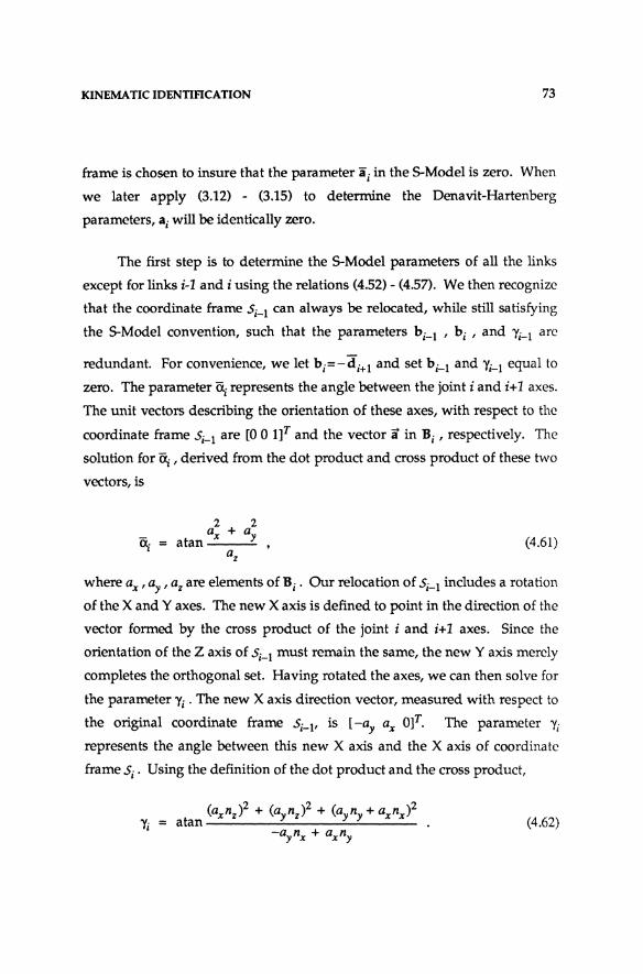
KINEMATIC IDENTIFICATION 73
frame is chosen to insure that the parameter ai in the S-Model is zero. When
we later apply (3.12) - (3.15) to determine the Denavit-Hartenberg
parameters, ai will be identically zero.
The first step is to determine the S-Model parameters of all the links
except for links i-1 and i using the relations (4.52) - (4.57). We then recognize
that the coordinate frame Si-} can always be relocated, while still satisfying
the S-Model convention, such that the parameters bi- 1 ' bi ' and 1i-l are
redundant. For convenience, we let bi=-dj+1 and set bi-} and 1j-l equal to
zero. The parameter ~ represents the angle between the joint i and i+ 1 axes.
The unit vectors describing the orientation of these axes, with respect to the
coordinate frame Si-l are [0 0 If and the vector it in Bj ,respectively. The
solution for ~ , derived from the dot product and cross product of these two
vectors, is
(4.61)
where ax' ay ' az are elements of Bj . Our relocation of Si-l includes a rotation
of the X and Y axes. The new X axis is defined to point in the direction of the
vector formed by the cross product of the joint i and i+ 1 axes. Since the
orientation of the Z axis of Sj_l must remain the same, the new Y axis merely
completes the orthogonal set. Having rotated the axes, we can then solve for
the parameter 1i . The new X axis direction vector, measured with respect to
the original coordinate frame Si-l' is [-ay ax Of. The parameter 1i
represents the angle between this new X axis and the X axis of coordinate
frame Si. Using the definition of the dot product and the cross product,
(4.62)

74 KINEMATIC IDENTIFICATION
The new Si-l coordinate frame is, in fact, the Denavit-Hartenberg link
coordinate frame 'Ii-I in Figure 3-2. Furthermore, the transformation be
tween Si-2 and Si is independent of the physical location of Si-l' This trans
formation is defined by the matrix product
Bi_IBi = Rot(z'~i_l )Trans(O,O,di_1 )Trans(ii"':I'O,O)
Rot (x, ~-l )Rot(z, 'Vi-I )Trans (0,0, b i_1 )Rot(z, ~i)
Trans(O,O,di)Trans(ii,O,O)Rot(x,~)Rot(z,ri)
Trans (0, 0, bi) , (4.63)
which is derived from (3.2). Setting b.=-d. 1 and'll. l=b. l=a.=O in (4.63) 1 1+ 1,- 1- 1
and rearranging yields
Rot (z, ~i-l )Trans (0, 0, d i-l )Trans (ai-I' 0, 0)
(4.64)
The left-hand side of (4.64) can be evaluated using the parameters iii and 'Vi
obtained from (4.61), (4.62), and (4.54), and the known matrices Bi-l and Bi .
Conversely, the right-hand side of (4.64) is a function of the unknown
parameters ~i-l ' di-l ' a i- 1 ' ~-1 ' ~i ' and d i · Upon comparison, the
right-hand side of (4.64) is functionally identical to that of the general trans
formation matrix in (3.2). Applying the appropriate substitutions to (4.52) -
(4.57), the solutions for the six the remaining unknown S-Model parameters
are:
~i-l
when a =a =0 x y
(4.65)

KINEMATIC IDENTIFICATION
i ~1
-a atan~
ay
-oxcosPi-l - 0ySinPi-l Pi = atan . '
nxcosPi-l + n" sm Pi-I
ai-I = PxcosPi_l + pysinPi_I '
-PxsinPi-l + pycosPi-l
sin~1
o
75
otherwise
(4.66)
(4.67)
(4.68)
if sin Dr-I * 0
(4.69)
(4.70)
where n" ' ny , nz ' 0" ' 0, ' az ' a" ' a, ' and az are the elements of the matrix defined by the left-hand side of (4.64). When two or more consecutive joints
are prismatic, the corresponding 5-Model link coordinate frames should be
relocated such that their origins coincide. Solutions for the nonzero S-Model
parameters, analogous to those in (4.65) - (4.70), can then be derived.
The Denavit-Hartenberg parameters 01 and d l are functions of the S
Model parameters 'Yo and bo ' respectively. In principle, 'Yo and bo can be
computed from the elements of the matrix Bo' From (4.51), however, Bo is
undefined since neither 5_1 nor equivalently S_1 is defined in our identifica
tion algorithm. Fortunately, 01 and d1 are not essential for the kinematic
modeling and control of manipulators. We circumvent the problem by
modifying the model in (2.8). We replace the matrix Til by Til to represent
the poSition and orientation of the nth link coordinate frame in terms of the

76 KINEMATIC IDENTIFICATION
identified S-Model base coordinate frame So' To distinguish between the
modified model and the original Denavit-Hartenberg model in (2.8), we ex-
press Tn as
Tn = Ar A2· .. · ·An = [Rot(z, -yo)Trans(O,O,-bo)]Tn (4.71)
where the matrix ~ ~ (ql) has the functional form of (2.9), and
Ai = Ai(iL) fori=2, ... ,no We replace ql by
(4.72)
for a revolute joint and
(4.73)
for a prismatic joint. We call the model in (4.71) the pseudo Denavit
Hartenberg model. Even though the parameters Yn and bn are not required
to formulate the pseudo Denavit-Hartenberg model in (4.71), we compute all
of the S-Model parameters in the third step of our identification procedure.
The parameters Yn and bn may be required to invert (4.71).
The model (4.71) describes the spatial relationship between a coor
dinate frame attached to the base of the manipulator and a coordinate frame
attached to the end-effector as a function of the joint positions as defined by
the joint encoders. Robot kinematic models, such as (2.8), (3.1), and (4.71),
only describe the internal kinematics of the device. The location of the link
coordinate frames with respect to physical points or surfaces on the mechani
cal linkages, is not specified by these models. In particular, the physical

KINEMATIC IDENTIFICATION 77
location of the base frame and the end-effector frame are unknown. In prac
tice, most robot manufacturers select the parameters of the design model so
as to insure that the base frame and end-effector frame coincide with certain
physical features of the base and end-effector <e.g., machined bosses or the
surface of a mounting flange). This, in principle, allows the users to
precisely locate the manipulator in a workcell and to program the robot
motions in terms of absolute coordinates. This approach to robot program
ming and control has numerous disadvantages.
The preferred approach is to generate task descriptions and control
programs which are independent of the manipulator. All motions of the
end-effector are referenced to an arbitrary coordinate frame called the task
coordinate frame. Prior to executing the task, the robot is taught the location
of the task coordinate frame. Thus, in the practical implementation of robot
tasks the absolute physical locations of the base frame and end-effector coor
dinate frames are not necessary.
The location of targets 1 and n, in the 5-Model identification algorithm,
determines where the base and end-effector coordinate frames lie. Their
location and the location of the remaining n-2 targets has, conceptually, no
affect upon identified internal kinematics of the manipulator. If, however,
the application demands that the robot be positioned in a particular refer
ence frame, the relationship between the base and end-effector frame must
be specified with respect to the physical device. This is accomplished by
mounting targets 1 and n at predefined locations which satisfy the necessary
physical constraints.

78 KINEMATIC IDENTIFICATION
4.4. Conclusions
The S-Model identification algorithm possesses the following features
for accurate kinematic parameter estimation and robot modeling:
• Since the 5-Model is an exact kinematic description, the estimated model approaches the ideal model as the measurement noise is reduced to zero. Simulation experiments have demonstrated this property of the model.
• The sensor system for measuring the position of the target point is independent of the robotic manipulator and eliminates the need for sophisticated fixturing and accurate placement of the manipulator. Acoustic and optical sensor systems for this application are commercially available.
• Placement of the target points on the robot is essentially arbitrary and requires only minor fixturing.
• Simple linear least-squares algorithms are applied to estimate the parameters. Solving a huge nonlinear minimization problem, as proposed by Whitney and Lozinski [30], is thus eliminated.
• One can calculate the standard Denavit-Hartenberg parameters from the 5-Model parameters.
• The effects of measurement noise upon the estimated parameters can be reduced by increasing either the number of target locations measured per circle (line) or the nominal target radius (for revolute joints).
• The approach leads to a robust algorithm for identifying the kinematic structure of all n degree-of-freedom robotic manipulators.
• The systematic structure of the algorithm leads to efficient and practical implementations requiring little or no operator interaction (as demonstrated by our implementation described in Chapter 6).

5.1. Overview
ChapterS
Inverse Kinematics
The inverse kinematic problem requires the solution of a set of n
coupled nonlinear equations. Since arm signature models do not possess
closed-form inverse kinematics, numerical methods must be applied to solve
the nonlinear equations. In this chapter, we describe two algorithms for
solving the inverse kinematic problem. The first algorithm, based upon
Newton's method, was originally proposed by Khosla, et al. [12]. We have
applied this algorithm in our hardware implementation and evaluation of
arm signature identification. The second algorithm is the Jacobi iterative
algorithm applied specifically to the inversion of signature models. In the
context of this dissertation, we consider the implementation of the inverse
kinematic equations to be synonymous with the robot's kinematic control
algorithms. Used by themselves to position the end-effector, the inverse
kinematic equations correspond to an open-loop control structure. Closed
loop or sensory feedback techniques are more appealing but the real-time
measurement of the end-effector's position and orientation is, in general,
impractical with current technologies. In this chapter, the term kinematic
control will be used instead of the term inverse kinematics.
80 INVERSE KINEMATICS
5.2. Newton-Raphson Algorithm
The kinematics of serially-connected robotic manipulators can be
described by the multiplicative matrix model
(5.1)
where the Ki matrix can be expressed as
if joint i is revolute (5.2)
or
if joint i is prismatic. (5.3)
The constant homogeneous transformation matrix ~ defines the constant
component of the transformation from the link i-l coordinate frame to the
link i coordinate frame. The matrix Tn defines the position and orientation of
the end-effector in terms of a coordinate frame fixed relative to the base of
the manipulator.
For kinematic control, our objective is to determine the joint coor
dinates 'f which correspond to the desired end-effector position and orien-• tation Tn=Tn. When the nonlinear equations in (5.1) are solved iteratively by
the Newton-Raphson algorithm [12], the solution at the (k+1) th iteration is
(504)
where J(qk) is the manipulator Jacobian evaluated at qk. The vector r; k
represents the differential translation and rotation between the position and
orientation of the desired end-effector location T: and the predicted end
effector location corresponding to q k= [q~ q~ ... q~]T defined in (5.1). The

INVERSE KINEMATICS 81
differential translation and rotation vector "8 k is defined in terms of the base
coordinates in (5.1). Any set of rotation angles with a predefined sequence of
rotations (e.g., Eu1er angles, roll-pitch-yaw, and Cartesian x-y-z) can be used
to define the rotational components of "8 k. The choice only affects the for
mu1ation of the manipulator Jacobian. Expressions for the manipulator
Jacobian in terms of the elements of the Ki matrices for different definitions
of "8 k are presented in [7, 18].
The Newton-Raphson algorithm (5.4) converges in theory when the
difference, Til (qk+l)_T: ' becomes zero. In practice, two approaches can be
taken to assess convergence. In the first, the algorithm is assumed to con
verge when each element of the above difference has reached a user
prescribed threshold. The second approach assumes that the algorithm has
converged when each component of the incremental change in the solution is
less than the resolution of the corresponding joint encoder. The latter ap
proach is easier to implement and takes into account the physical1imitations
of the device itself.
Application of numerical methods to solve the inverse kinematic
problem gives rise to the following issues:
• Selection of an initial estimate
• Rate of convergence
• Convergence to the desired solution
• Presence of singularities
Selection of an initial estimate, in our application, is relatively simple. Since
the robot design and identified signature models are nearly identical in
terms of predicting end-effector position and orientation, we apply the
design model to initialize qo. Our initial estimate qO is then the inverse

82 INVERSE KINEMATICS
solution of the design model evaluated at the desired end-effector location • Tn' The number of iterations required for (5.4) to converge is directly related
to the accuracy of the initial estimate. Since the initial estimate obtained
from the design model is close to the true solution, we require only a few
iterations. In our experimental evaluation of the Newton-Raphson algorithm
we have found that the algorithm converges to the true solution within 2-3
iterations.
Fully articulated manipulators, such as the Puma 560, possess multiple
inverse kinematic solutions. These multiple solutions differ by such physical
characteristics as the right and left shoulder configurations of the Puma 560.
For kinematic models with closed-form inverses, a parameter to specify the
unique characteristics of a desired solution can be incorporated explicitly
into the inverse algorithm. This approach, however, does not apply to
kinematic models without closed-form inverse solutions. Consequently, the
issue arises as to how to insure that the iterative solution converges to the
desired solution. Since our initial estimate, which is derived from a closed
form inverse model, is close to the true solution, we select the initial estimate
to be of the configuration of the desired solution.
The Newton-Raphson algorithm has two practical disadvantages.
First, it requires the evaluation of the inverse Jacobian at each iteration. In
version of the Jacobian matrix is a major contributor to its computational
complexity. If the desired end-effector position T: corresponds to a joint
configuration which is close to being degenerate, the algorithm in (5.4) be
comes numerically unstable (Le., the Jacobian matrix becomes singular).
Degenerate or near-degenerate configurations can almost always be avoided
by modifying the robot trajectory planner. This approach often reduces
manipulator dexterity and programmability, thereby limiting the range of
applications to which the robot can be applied. Second, the Newton-

INVERSE KINEMATICS 83
Raphson algorithm requires a significant number of multiplications, ad
ditions, and trigonometric function calls at each iteration (refer to Section
5.5). Computationally intensive operations include generation of the
Jacobian elements, and evaluation of (5.1) and the elements of 8 k. The
Newton-Raphson algorithm is more computationally complex than the
closed-form inverse solution typically applied to kinematic control.
5.3. Jacobi Iterative Method
The extent to which arm signature identification and control is applied
to improve robot positioning performance will, in part, be determined by the
computational complexity of the signature control algorithm. In this section,
we apply the Jacobi iterative algorithm to invert arm signature models as an
alternative to the computationally complex Newton-Raphson algorithm. In
contrast to the Newton-Raphson algorithm, the Jacobi iterative algorithm
explicitly incorporates the knowledge of both the robot design and the sig
nature models.
We introduce the following notation. Let the forward kinematics, ac
cording to the design model, be denoted by T,!=Fd(ct) and the inverse
kinematic model by q=F~l<T,!). Similarly, let the forward kinematics, ac
cording to the signature model, be denoted by ~=Fs(q) and the inverse
kinematic model by q=F~l~). Finally, let
(5.5)
Our objective is to determine the joint coordinates if so that Fs{q·) is • equal to the desired end-effector position and orientation Til (i.e., to compute
it =F~l (T:». We premultiply both sides of (5.5) by [Fs(q)r1 and the result
by the design model Fd(q) to obtain

84 INVERSE KINEMATICS
(5.6)
By applying the inverse design kinematic model relationships F~l (cD to both
sides of (5.6), we obtain the fixed point equation
(5.7)
We thus seek the joint coordinates if which are the fixed point of the right
hand side of (5.7) [9]. According to the Jacobi iterative algorithm, we can
obtain a solution by iterating the right-hand side of (5.7). The Jacobi iterative
algorithm is
(5.8)
which is initialized by setting if= F~l(T:). We select the initial estimate to be
of the configuration of the desired solution as we did for the Newton
Raphson algorithm.
The algorithm (5.8) has a relatively simple physical interpretation. In
Figure 5-1, we represent the end-effector positions and orientations defined
by the matrices Fs(qk), Fd(qk), and T: by three generic vectors in six dimen
sions. The vector denoted by Ak in Figure 5-1 represents the difference be
tween the solution at the k th iteration and the desired solution, measured in
Cartesian space. Analytically, Ak is the product
(5.9)
contained in (5.8) and is the error term which drives the algorithm towards
the solution. The new Cartesian position and orientation

INVERSE KINEMATICS 85
Figure 5-1: Physical Interpretation of the Jacobi Iterative Algorithm
(5.10)
in (5.8) is then input to the inverse design kinematic model to compute the
new solution qk+l. At each iteration, the location 1* is translated and rotated
by the same amount as the error between the desired and signature model
end-effector locations. Implicitly, the algorithm searches for the end-effector
location 1* corresponding to T: such that
-1 k -1· Fd (T ) = Fa (T,.) . (5.11)
In the Jacobi algorithm, the design model Fd(qk) and the signature model
Fs(qk) must both be expressed in terms of the same physical base coordinate
frame as illustrated by the common origin in Figure 5-1.
We have applied this algorithm in simulation to invert signature

86 INVERSE KINEMATICS
models. Our simulations demonstrate that the algorithm in (5.8) converges
to the true solution if if the product
(5.12)
is close to the identity matrix. The matrix P (en is the transfonnation be
tween the end-effector position and orientation predicted by the design and
the signature models. Since robot manufacturing errors are small in com
parison with the physical dimensions of the robot, the mappings between the
joint and Cartesian spaces defined by the two models will, in practice, be
similar. Hence, for joint configurations qk in the vicinity of if, the model
mismatch (5.12) will vary only slightly in comparison to the workspace of the
manipulator (e.g., for the Puma 560, typical values for the model mismatch
are on the order of 0.5 mm and 0.1 degrees).
Henrici [9] has shown that the Jacobi iterative algorithm is guaranteed
to converge if the function on the right-hand side of (5.7) is a continuous
contraction mapping. While we cannot prove that this function is a con
tinuous contraction mapping due to the analytic complexity of the design
and signature models and the inverse design model, the simulations il
lustrate the fact that the Jacobi iterative algorithm has a linear rate of conver
gence and that the Newton-Raphson algorithm has a quadratic rate of con
vergence. We assume that the algorithm has converged when all the com
ponents of the incremental change in the solution are less than the resolution
of their corresponding joint encoder. In all of our simulations, the Jacobi
iterative algorithm converged to the solution (within the limits of the Puma
560 joint encoders) within at most 9 iterations while the Newton-Raphson
algorithm required 3-4 iterations to converge to an equally accurate solution.
The algorithm in (5.8) requires matrix multiplication, evaluation of the

INVERSE KINEMATICS 87
closed-form inverse of a homogeneous transformation matrix, and the evalua
tion of the inverse design model. Since homogeneous transformation
matrices are orthogonal, their closed-form inverses are written by inspection.
Even though the Newton-Raphson algorithm requires fewer iterations than
the Jacobi iterative algorithm to converge, our simulations indicate that the
reduced number of iterations may not offset their additional complexity.
Computationally, the Newton-Raphson and Jacobi Iterative algorithm are
both significantly more complex than the closed-form inverse model for a
Puma 560. In Sections 5.4 and 5.5, we evaluate the comparative performance
and real-time applicability of the Newton-Raphson and Jacobi Iterative al
gorithms. The computational complexity, the rate of convergence, and the
effects of reduced precision computation upon the performance of these al
gorithms will be among the features to be compared.
5.4. Performance Evaluation
Our evaluation of the performance of the Newton-Raphson algorithm
(5.4) and the Jacobi Iterative algorithm (5.8) consists of comparing their rates
of convergence and the effects of reduced precision computation. The con
vergence of the control algorithms depends upon the overall mismatch be
tween the design and signature models and the desired end-effector position
and orientation. In simulation, we applied both algorithms to numerically
invert identified arm signature models of a perfectly manufactured Puma
560 robot (i.e., the manufacturing errors are assumed zero). The identified
arm signature models of the Puma 560 were obtained from a simulator
(described in Chapter 7). With this second simulator, we identified arm
signatures of varying accuracy.
Each control algorithm was used to invert three different signature
models for n different desired end-effector locations (i.e., the input to the

88 INVERSE KINEMATICS
control algorithm}. The three signature models span a wide range in ac
curacy as determined by the magnitude of simulated measurement noise.
The n end-effector locations are chosen to span the full range of the Puma
560's workspace. At each iteration of each algorithm, we compute the error
/}"k with respect to the base coordinates. The orientational component of the
error is expressed in terms of Euler angles. We also compute the radial
position error as the Euclidean norm of the X, Y, and Z axis translational
errors. The four translational errors and three rotational errors were com
puted during each iteration of the two algorithms for the three signature
models and the various end-effector locations.
For all cases tested, the behavior of the two algorithms was qualita
tively equivalent. As the accuracy of the identified signature model in
creased the number of iterations required by both algorithms to converge
decreased. In all but a few cases, the three orientational and four trans
lational measures of the error term /}"k converged asymptotically. The dif
ference between the solutions obtained using single precision arithmetic ver
sus double precision arithmetic was insignificant6. Tables 5-1 and 5-2 list the
components of the error between the desired end-effector location and the
end-effector location computed using the solution at each iteration for the
Newton-Raphson algorithm and the Jacobi Iterative algorithm, respectively.
Table 5-1 illustrates the quadratic convergence of the Newton-Raphson
algorithm as compared to the linear convergence of the Jacobi algorithm in
Table 5-2. In this example, the Jacobi algorithm required nine iterations to
converge while the Newton-Raphson algorithm required only four. The
errors listed in Tables 5-1 and 5-2 were computed using the same identified
60ur simulations were conducted on a Digital Equipment Corporation VAX 11/780 and implemented in the C Programming Language.
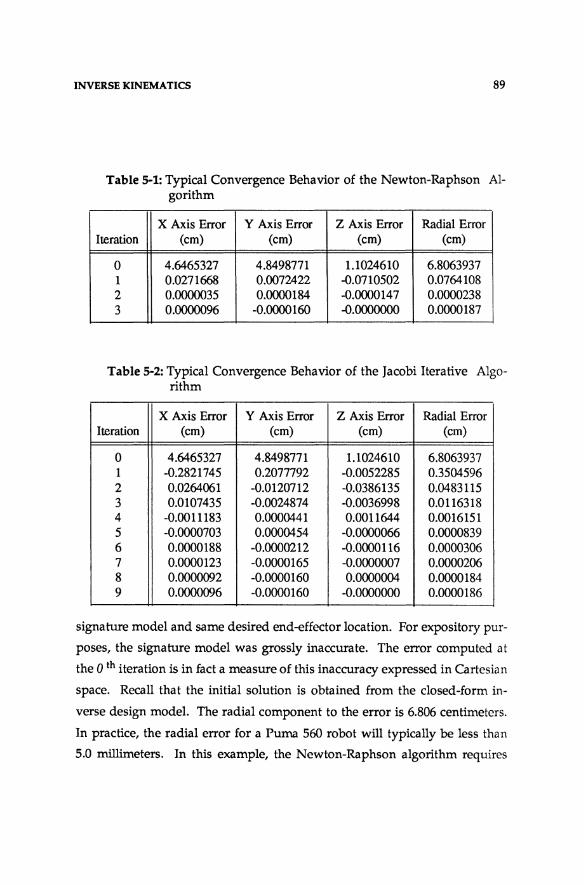
INVERSE KINEMATICS 89
Table 5-1: Typical Convergence Behavior of the Newton-Raphson Algorithm
X Axis Error Y Axis Error Z Axis Error Radial Error Iteration (em) (em) (em) (em)
0 4.6465327 4.8498771 1.1024610 6.8063937 1 0.0271668 0.0072422 -0.0710502 0.0764108 2 0.0000035 0.0000184 -0.0000147 0.0000238 3 0.00000% -0.0000160 -0.0000000 0.0000187
Table 5-2: Typical Convergence Behavior of the Jacobi Iterative Algorithm
X Axis Error Y Axis Error Z Axis Error Radial Error Iteration (em) (em) (em) (em)
0 4.6465327 4.8498771 1.1024610 6.8063937 1 -0.2821745 0.2077792 -0.0052285 0.3504596 2 0.0264061 -0.0120712 -0.0386135 0.0483115 3 0.0107435 -0.0024874 -0.0036998 0.0116318 4 -0.0011183 0.0000441 0.0011644 0.0016151 5 -0.0000703 0.0000454 -0.0000066 0.0000839 6 0.0000188 -0.0000212 -0.0000116 0.0000306 7 0.0000123 -0.0000165 -0.0000007 0.0000206 8 0.0000092 -0.0000160 0.0000004 0.0000184 9 0.0000096 -0.0000160 -0.0000000 0.0000186
signature model and same desired end-effector location. For expository pur
poses, the signature model was grossly inaccurate. The error computed at
the 0 th iteration is in fact a measure of this inaccuracy expressed in Cartesian
space. Recall that the initial solution is obtained from the closed-form in
verse design model. The radial component to the error is 6.806 centimeters.
In practice, the radial error for a Puma 560 robot will typically be less than
5.0 millimeters. In this example, the Newton-Raphson algorithm requires

90 INVERSE KINEMATICS
approximately 2 iterations to converge while the Jacobi algorithm requires
approximately 3-5 iterations. Based upon the results of numerous simula
tions, we conclude that both algorithms are numerically stable and extremely
robust.
In the next section, we analyze the computational complexity of the
Newton-Raphson and Jacobi Iterative algorithm and assess their real-time
applicability.
5.5. Comparative Computational Complexity
The computations required by the closed-form inverse design model
(in Appendix B) for a Puma 560 are outlined in Table 5-3.
Table 5-3: Computational Complexity of the Closed-Form Inverse Kinematic Model of the Puma 560 Robot
Variable atan2 sin cos + x -r-91 2 0 0 3 2 1
93 I I 1 5 5 1
923 1 1 1 4 6 0
92 0 0 0 1 0 0
94 1 0 1 3 7 0
95 1 0 1 2 5 0
96 I 0 1 7 15 0
Total 7 2 5 25 40 2
The first column indicates the joint position or sum of joint positions to
which the operations correspond. Similarly, the computations required by

INVERSE KINEMATICS 91
one iteration of the Newton-Raphson algorithm and one iteration of the
Jacobi Iterative algorithm for a Puma 560 are outlined in Tables 5-4 and 5-5,
respectively.
Table 5-4: Computational Complexity of One Iteration of the NewtonRaphson Algorithm
Step sin cos + x I
I 6 6 172 266 0
2 0 0 12 0 0
3 0 0 6 9 0
4 0 0 27 36 0
5 0 0 0 0 0
6 0 0 45 45 15
7 0 0 6 0 0
8 0 0 0 0 0
Total 6 6 268 356 15
The Newton-Raphson algorithm and the Jacobi algorithm are described in
terms of a sequence of steps. The eight steps of the Newton-Raphson algo
rithm and the six steps of the Jacobi algorithm are defined in Appendix C.
The total number of operations for one iteration of each algorithm are also
listed in the tables. The total complexity of each algorithm is obtained by
multiplying these totals by an upper bound for the number of iterations
required for convergence. The most computationally intensive step in the
Newton-Raphson algorithm is the evaluation of the inverse jacobian. The
majority of the computations involved in this task actually pertain to
evaluating the forward signature model.

92 INVERSE KINEMATICS
Table 5-5: Computational Complexity of One Iteration of the Jacobi Iterative Algorithm
Step sin cos atan2 + x ~
1 6 6 0 0 0 0
2 0 0 0 154 236 0
3 0 0 0 22 50 0
4 0 0 0 6 9 0
5 0 0 0 54 72 0
6 2 5 7 25 40 2
Total 8 11 7 261 407 2
The execution times of the Motorola 68020 microprocessor hard ware
instructions with a 68881 floating point co-processor are listed in Table 5-6
[16, 17].
Table 5-6: Execution Times of the Motorola 68020 with a 68881 Floating Point Co-Processor (12-MHz Clock)
Function Time (J.l.S)
Multiply 9.42
Add 7.75
Divide 12.08
Square Root 12.25
Sine 35.92
Cosine 35.92
Arc Tangent 36.92
The times listed in Table 5-6 are based upon a 12 megahertz clock frequency.
INVERSE KINEMATICS 93
These floating point operation times, including the times required to load
and store the operand, are used to estimate the time required to compute the
inverse kinematic solution. The execution times of the 68020/68881 are rep
resentative of the computational capabilities of microprocessors currently
being applied to robot control. The estimated computation time for the
closed-form inverse model is 1.1 ms. In contrast, the Newton-Raphson algo
rithm requires 17.77 ms (assuming three iterations to converge) and the
Jacobi algorithm requires 33.99 ms (assuming five iterations to converge).
The cycle time for the Puma 560 is 28.0 ms7 corresponding to a sample
rate of 39 Hz. During each cycle, the trajectory planner inputs an end
effector location to the kinematic controller which must then compute the
inverse solution and output the result to the various joint servo controllers.
The estimates indicate that the Newton-Raphson is implementable in real
time using commercially-available hardware whereas the Jacobi Iterative al
gorithm is not. The Newton-Raphson algorithm is computationally more
efficient than the Jacobi Iterative algorithm in terms of a direct single proces
sor implementation. However, the Jacobi algorithm does have a potential
advantage over the Newton-Raphson algorithm. The evaluation of the for
ward signature model in Step 1 of the Jacobi algorithm involves numerous
operations which can be performed in parallel. With the proper hardware,
significant reductions in the computation time can be realized. A cursory
examination suggests that the time required to perform the operations con
tained in steps 1 through 5 of the Jacobi Iterative algorithm can be reduced
by a factor four yielding a total computation time of approximately 12.6 ms.
This is not the case for the Newton-Raphson algorithm where the evaluation
of the forward signature model must be performed sequentially to provide
7 A recent update to the Puma 560 controller includes an 8 ms cycle time.

94 INVERSE KINEMATICS
the intermediate results necessary for computing the elements of the inverse
Jacobian matrix.
5.6. Conclusions
In this chapter, two numerical algorithms for solving the inverse
kinematic problem have been presented, namely, the Newton-Raphson algo
rithm and Jacobi Iterative algorithm. The results of numerous simulations,
indicate that both algorithms are numerically stable and extremely robust.
In our experiments, we have found that the Newton-Raphson algorithm con
verges to the true solution within 2-3 iterations while the Jacobi Iterative
algorithms typically converges within 7-9 iterations.
Computationally, the Newton-Raphson and Jacobi Iterative algorithm
are both significantly more complex than the closed-form inverse model. In
fact, the closed-form inverse solution is applied in both cases to provide the
initial estimate with which to begin. Based upon a serially programmed
single processor architecture, the Jacobi Iterative algorithm requires sig
nificantly more computation time than does the Newton-Raphson algorithm.
Based upon the execution times of the Motorola 68020 microprocessor with a
68881 floating point co-processor the Newton-Raphson solution takes ap
proximately 17.77 ms to compute and the Jacobi Iterative solution takes ap
proximately 33.99 ms. Since the cycle time of a Puma 560 robot is 28.0 ms,
the Newton-Raphson algorithm is implementable in real-time using
commercially-available hardware.
The Jacobi Iterative algorithm has two distinct advantages over the
Newton-Raphson algorithm. First, it is easier to program. The Newton
Raphson algOrithm, for instance, requires separate algorithms just to invert
the 6x6 manipulator jacobian. Second, the Jacobi Iterative algorithm involves

INVERSE KINEMATICS 95
numerous operations which can be performed in parallel which, with the
proper processor architecture, could significantly reduce the overall com
putation time. A rough estimate suggests a total computation time of ap
proximately 12.6 ms which is less than the Newton-Raphson algorithm. The
recent development of customized processors for robotic applications is ex
pected to further reduce the computation time.
In the next chapter, we demonstrate both the feasibility and practicality
of arm signature identification and control by applying the S-Model iden
tification and Newton-Raphson algorithms in proof-of-concept hardware ex
periments to improve the performance of seven Puma 560 robots.

Chapter 6
Prototype System and Performance Evaluation
6.1. Overview
In order to demonstrate the feasibility and evaluate the performance of
the identification and control algorithms, we have developed a complete
prototype system. This prototype arm signature system has been applied to
identify and control seven Westinghouse/Unimation Puma 560 robots. 8.
The Puma 560 is a six degree of freedom robot with revolute joints. Evalua
tion of the arm signature-based control showed consistent improvement of
accuracy in several standard tasks.
In this chapter, we describe the hardware/software implementation of
the identification and control algorithms and describe the evaluation of
kinematic performance.
8Puma is a trademark of the Weslinghouse/Unimation Corporation

98 PROTOTYPE SYSTEM AND PERFORMANCE EVALUA nON
6.2. System Overview
Figure 6-1 illustrates the configuration of the hardware components in
the implementation. Figure 6-2 is photograph of the system with the target
sparker for Joint 6 mounted in the bar on the end-effector. The sensor array,
described in Section 6.3.1, is a rigid fixture which supports four ultrasonic
microphones. In the figure, the microphones are labeled as A, B, C, and
D. The sensor array also supports to calibration rods indicated by the two
sets of parallel lines which intercept with microphones Band
D. Microphones A, B, and C form an approximate right triangle with vertex
at microphone B. The sensor array is mounted on a wall such that the active
volume of the sensor array and the workspace of manipulator which is
mounted on a table coincide. The sensor array in combination with the
GP-8-3D sonic digitizer are used to measure the straight line distances be
tween the microphones and the target points attached to the robot. These
measurements, called slant ranges, are then used to determine the Cartesian
position of the target points based upon triangulation. The ultrasonic
digitizer is interfaced to the Puma Controller using an RS-232 serial line
which is itself interfaced to a V AX 11/780 using another RS-232 serial line.
The software which controls the Puma 560 during the collection of the
raw target slant ranges is implemented on the Puma's Val II Controller and
is written in the Val II programming language [27,28]. This program is
initially downloaded from the V AX 11/780 which maintains current versions
of all the system software and provides permanent storage for all experimen
tal data. The software which implements the slant range compensation and
target triangulation algorithms (Appendix E.2) is written in the C program
ming language to run under the Unix9 operating system on the Digital
9Unix is a trademark of AT&T Bell Laboratories, Murray Hill, NJ.

PROTOTYPE SYSTEM AND PERFORMANCE EVALUATION
UNIMATE CONTROLLER
PDP 11/73
RS-232
Sensor Array
Upload/Download Line
RS-232
Figure 6-1: Hardware Configuration
99
VAX 11 780
(UNIX)
RS-232
Teach Pendant

100 PROTOTYPE SYSTEM AND PERFORMANCE EV ALUA TION
Figure 6-2: Arm Signature Identification System and Puma 560 Robot.
Used with permission from the Robotics Institute at Carnegie-Mellon University, copyright 1987. Photo taken by Mary Jo Dowling.

PROTOTYPE SYSTEM AND PERFORMANCE EVALUATION 101
Equipment Corporation VAX 11/780 [11]. The slant range measurements
are thus collected by the VAL II controller and then uploaded to the VAX
11/780. The software which implements the feature parameter estimation
and computes the signature parameters is also written in the C programming
language and runs on the VAX 11/780. Once identified, the arm signature is
stored for future use to control the manipulator.
The closed-form inverse kinematics of the Puma 560 (refer to Appendix
B.2) and the Newton-Raphson algorithm (in Section 5.2) are implemented in
the C programming language on the VAX 11/780. We apply both the
closed-form inverse kinematic model and Newton-Raphson algorithm to
solve for the joint configurations corresponding to desired Cartesian loca
tions of the end-effector and to control the robot in a variety of tasks. The
tasks used to analyze manipulator kinematic performance and the in
strumentation required to obtain the pertinent measurements are described
in Section 6.5.
6.3. Sensor System
The sensor system measures the three-dimensional positions of targets
attached to the robot arm. We use an ultrasonic source (sparker) for each
target and an array of four ultrasonic range detectors to estimate target posi
tions. Each detector measures time-of-flight independently from the target
and computes an estimated range. Knowing the geometry of the detector
configuration the three-dimensional coordinates of the point may be es
timated.

102 PROTOTYPE SYSTEM AND PERFORMANCE EVALUA nON
6.3.1. Description
The GP-8-3D Sonic Digitizer (manufactured by the Science Accessories
Corporation) is an ultrasonic range sensing system which computes range
measurements based upon the time of flight of an ultrasonic wave emitted
from a source to a set of receiving microphones [22]. The primary com
ponents of the GP-8-3D Sonic Digitizer are
• A controller
• A multiplexer
• Four ultrasonic piezo-electric transducers (microphones)
• Eight emitters (sparkers)
The interconnection of these components is illustrated in Figure 6-3.
Parallel Interface
Power;., ;4~--~----~~
123456
Sparkers
Figure 6-3: GP-8-3D Sonic Digitizer Components
The controller, equipped with an RS-232 serial port, can be interfaced to a
PROTOTYPE SYSTEM AND PERFORMANCE EVALUATION 103
host computer to allow for remotely-controlled digitizing and data acquisi
tion. In our application, the host computer is the PDP 11/73 in the Puma 560
Controller. Using the multiplexer, the range measurements to anyone of
eight different sparkers can be obtained. The GP-8-3D controller has four
input channels, one for each microphone. When requested to digitize, the
GP-8-3D initiates a control signal which simultaneously triggers the desired
sparker to spark and resets four counters.
When the sound wave emitted by the sparker reaches a microphone a
level detector is triggered, and the time of flight is recorded. The velocity of
sound at ambient temperature is used to compute the estimated range from
the time-of-flight and the computed slant ranges are then transmitted to the
Puma 560 Controller via the RS-232 serial line.
Our sensor system utilizes five sparkers and four microphones. For
identification purposes, the sparkers are numbered 1 through 5 and the
microphones are labeled A through D. Sparker 5 represents the target
sparker which is attached to each of the links of the manipulator during the
identification process. The remaining sparkers and the microphones are
mounted at fixed locations relative to one another as illustrated in Figure 6-4.
The locations of microphones A, B, and C define the sensor plane. The sensor
system is mounted on a wall such that the sensor plane is perpendicular to
the ground and the line joining microphones A and C is approximately
horizontal. In our implementation, the distances between microphones A
and B, Band C, and A and C are nominally 143.0 cm, 143.0 cm, and 203.0 cm,
respectively. The active volume of the sensor array depicted in Figure 6-4 is
a cube approximately 143.0 cm on a side with vertices at microphones A, B,
andC.
The Cartesian coordinates of the target sparker, Sparker 5, obtained

104 PROTOTYPE SYSTEM AND PERFORMANCE EV ALUA nON
Sparker 2
Z Axis
Out of Page
Lower Calibration Rod
Figure 6-4: Sensor Configuration and Orientation
Vertical
t
through triangulation, are referenced to a Cartesian coordinate frame im
plicitly defined by the location of Microphones A, B, and C. This reference
frame is the Sensor Coordinate Frame depicted in Figure 6-4. Its origin coin
cides with the acoustic zero point of Microphone C. The Y axis is directed
along the line joining the acoustic zero points of Microphones C and B. The Z
axis is perpendicular to and out of the plane defined by the acoustic zero
points of Microphones A, B, and C. The X axis, formed by the vector cross
product of the Y and Z axis unit direction vectors, completes the orthogonal
set.
The GP-8-3D ean measure slant ranges between 30 em and 250 em with
a resolution of .01 cm. The accuracy of the computed slant ranges, however,
varies significantly, depending upon the environmental operating con
ditions. The speed at which sound travels in air is primarily a function of

PROTOTYPE SYSTEM AND PERFORMANCE EVALUA nON 105
temperature, humidity, altitude, frequency, barometric pressure, and air
flow. The speed of sound is particularly sensitive to variations in tempera
ture (1281.4.4 cm/secrF at 70.0 OF). For instance, if the actual temperature
of the air between a microphone and the sparker is 69.0 OF instead of the
assumed 70.0 OF, the GP-8-3D would measure a 150.0 em slant range as
155.79 cm. In general, differences between the actual and nominal operating
conditions produce a difference between the actual and nominal speed of
sound and hence, reduce the accuracy of the computed slant ranges. The use
of multiple sparkers and a special sensor array design enable us to compen
sate the slant range measurements taken by the GP-8-3D for variations in the
speed of sound (refer to Appendix E). This greatly increases the Cartesian
accuracy of the overall sensor system.
Following the compensation procedure described in Appendix E, the
final estimates for the three primary slant ranges sl ' s2 ' and s3 representing
the distances between the target sparker and Microphones A, B, and C,
respectively, are applied to determine the Cartesian coordinates of the target.
Upon triangulating, the X, Y, and Z coordinates of the target are computed
according to
x rcos(e) + rtan 2(e) cos (e) - y
= tane (6.1)
(wB C)2 + (83)2 - (82)2 Y =
2WB,C (6.2)
z = "';(83)2 -Xl-y2 (6.3)
where
(wA,a2 + (83)2 - (81)2 r =
2WA,C (6.4)

106 PROTOTYPE SYSTEM AND PERFORMANCE EVALUATION
cos (9) (wA,c)2 + (wB,cY - (w A,B)2
(6.5) = 2wACw BC . ,
tan (9) (1 - cos 2(9»2
(6.6) = cos (9)
and wA,B' wB•C ' and wA•C are the distances between Microphones A and B, B
and C, and A and C, respectively. The coordinate relations (6.1) - (6.3) can be
simplified if the triangle fonned by Microphones A, B, and C is a perfect
right triangle.
6.4. Generating Features
The 5-Model Identification algorithm leads to an efficient and well
defined method for collecting measurements. We sequentially attach a
sparker to each link of the Puma robot to implement the target points
described in Section 4.3.2. The fixtures used to attach the sparker to a link
are simple both in design and construction. For example, consider the fix
ture illustrated in Figure 6-5 which supports the sparker to Link 6 im
plementing Target Point 6. The two requirements for this fixture are that it be
rigid and that the distance between the sparker and the Joint 6 axis be ap
proximately equal to R6 ' where R6 depends upon the active volume of the
sensor system. We call R j the nominal radius of target point i. The nominal
radii for the six target points in our implementation are listed in Table 6-1.
In general, increasing the nominal radii increases the accuracy of the
identified planes-of-rotation.
We begin the measurement process by positioning the manipulator in
the desired signature configuration using a teach pendant. Conceptually, the
signature configuration can be any arbitrary configuration. However, in
practice, the signature configuration may depend upon the characteristics of

PROTOTYPE SYSTEM AND PERFORMANCE EVALUATION
Rectangular Aluminum Bar (Brazed to Aluminum Plate)
~~~~j Mounting Screws
Link 6 Face Plate
107
Sparker in Brass Sleeve
Figure 6-5: Fixture for Attaching Target Point 6 to link 6
Table 6-1: Puma 560 Target Point Nominal Radii
Target Point Nominal Radius (em)
1 40.87
2 41.62
3 43.71
4 33.30
5 45.13
6 33.30
the sensor system. In our implementation, we must insure that the lines of
sight between the target sparker and the three Microphones A, B, and C
remain unobstructed. Requirements such as this may also affect the design
of the mounting fixtures and the selection of the target point's positions with
respect to the links. The signature configuration we have selected is il
lustrated in Figure 6-6.The angular positions of the joints which define the
signature configuration are measured and recorded. We denote the sig
nature configuration by the vector q"= [q~,q;, ... ,q~]T. In Figure 6-6, q S is
nominally [155.0 179.0 178.00.00.0 O.O]T.

108 PROTOTYPE SYSTEM AND PERFORMANCE EVALUA nON
Figure 6-6: Approximate Signature Configuration for the Puma 560
We independently and incrementally vary the position of each joint of
the manipulator such that the six target points generate circular trajectories
in space. At each fixed configuration of the manipulator, we measure and
record the set of seven slant ranges required to determine the Cartesian
position of the target sparker. To further improve the estimates of measured
target positions, we measure and record several sets (typically 10-20) of
seven slant ranges at each configuration. Random fluctuations in the
measured slant ranges are then reduced through averaging.
The measured target positions represent sample points on the
generated circular trajectories. Six sets of points are obtained, each set cor
responding to the trajectory of a distinct target point. The measured target
positions will be used to identify 12 kinematic features, six planes-of-rotation
and six centers-of-rotation, which are then applied to construct the set of

PROTOTYPE SYSTEM AND PERFORMANCE EVALUATION 109
S-Modellink coordinate frame transformation matrices Si for i=l, ... ,6. To
identify the manipulator's kinematic parameters, the matrices Si must
represent the position and orientation of a set of S-Model link coordinate
frames when the manipulator is in the specified signature configuration.
Consequently, while taking measurements of the i th target's position, joints
1 - i-1 must remain in their respective signature configuration positions (Le.,
ql =q~, q2=q~, ... , qi-l =q~-l)' The positions of joints i+1 - 6 have no effect
upon the position of the i th target point since it is assumed to be rigidly
attached to the i th link., Joints i+1 - 6 are positioned so as not to limit the
motion of joint i or obstruct the lines of sight between the target and the
sensor array.
We have established a systematic method for indexing the configura
tion of the manipulator to insure that the previous conditions are satisfied.
Figure 6-7 is a flow chart indicating the sequence of operations in this
method. Measurements of the position of Target Point 6 are first qbtained,
followed successively by those of Target Points 5, 4, 3, 2, and 1. In Figure 6-7,
Ni denotes the number of distinct positions of joint i at which the position of
target i is measured and Nallg denotes the number of slant range measure
ments averaged at each target position. Increasing Ni typically increases the
accuracy of the estimated feature parameters. In Section 6.5 we explore the
relationship between Ni and the arm signature accuracy. We have identified
signatures using as few as five measurements per circle and as many as 100.
Each identified arm signature is based upon
6
L 7Nallg-Ni i=l
(6.7)
raw slant range measurements. For instance, if Ni=l00 for i=l, ... ,6 and
Nallg = 10, then 42,000 slant range measurements will be required. We are
able to obtain these measurements using the hardware in Figure 6-1 in ap-

110 PROTOTYPE SYSTEM AND PERFORMANCE EVALUATION
max max q ,q
1 2
w , w , w
min q 6
max q
6
A,B B,C A,C
Place robot in Signature Configuration
Place joints i, i+1, •.• , 6
in desired arbitrary configuration
k - 0, 1, ••• , N
q ....... q + j j
max min (qj -q )/N-1
j i
Figure 6-7: Flow Chart of the Algorithm for Collecting Target Point Measurements

PROTOTYPE SYSTEM AND PERFORMANCE EV ALUA nON 111
proximately 1 1/2 hours. This includes the time required to manually switch
the target sparker from one target point fixture to the next. The algorithm
described in Figure 6-7 is implemented in the VAL II programming lan
guage.
6.5. Measuring Performance
We have devised three methods for measuring manipulator kinematic
performance and have applied these methods to evaluate the performance of
the seven Puma 560 robots. Each method has an associated task which is
performed by the robot. These are
• The one-dimensional grid touching task
• The two-dimensional grid touching task
• The three-dimensional grid touching task
During these tasks, the manipulator is programmed to sequentially position
its end-effector at the vertices of a one-, two-, or three-dimensional grid
defined with respect to the workspace coordinate frame. At each of the grid
points, the actual relative position of the end-effector with respect to the
workspace coordinate frame is measured. Measurements of the end
effector's position, with respect to the robot's base coordinate frame cannot
be obtained since the physical location of the base frame has not been deter
mined in the signature analysis. The Cartesian positioning accuracy of a
robot with respect to a workspace coordinate frame is most useful in applica
tions.
The Puma is initially taught three arbitrary points to define a
workspace coordinate frame. The corresponding joint configurations are
denoted by the vectors "if1, "if2, and "if3• These configurations are recorded by

112 PROTOTYPE SYSTEM AND PERFORMANCE EV ALUA nON
the Puma Controller. The position and orientation of the end-effector, with
respect to the base coordinate frame for each of these configurations, are
computed using the appropriate forward kinematic model (Le., either the
signature model or the design model). The origin of the workspace coor
dinate frame is defined to be coincident with the position of the end-effector
at Point 1. The X axis is parallel to the line joining the end-effector's position
at Points 1 and 2. The Z axis is normal to the plane defined by the position of
the end-effector at Points 1, 2, and 3. Finally, the Y axis completes the
orthogonal set. Using this procedure, it is relatively easy to align the
workspace coordinate frame with a desired physical coordinate frame such
as that defined by the surface of a table.
Our objective is to measure positioning errors resulting from the mis
match between the actual and identified kinematics and the actual and
design kinematics. The positioning errors which occur while a robot is in
motion are both a function of the kinematic errors and the dynamic control
system errors. Consequently, measurements of the end-effector's positions
are taken only when the manipulator is stationary in specified fixed con
figuration. The Puma's steady-state joint positioning errors are typically
within ± I encoder count (± .005 degrees) of the desired positions.
6.5.1. One-Dimensional Grid
The objective in the one-dimensional grid touching task is to determine
the accuracy with which the robot can displace its end-effector. The robot is
programmed to touch two points in space. The location of these points is
specified in terms of Cartesian coordinates and defined with respect to a
previously taught workspace coordinate frame. Conceptually, these points
represent the endpoints of a traced line. We attach a pushpin to the end
effector and measure the actual distance between the tip of the pin at the two
points with a cathetometer. Figure 6-8 illustrates the measurement process.

PROTOTYPE SYSTEM AND PERFORMANCE EVALUATION 113
Figure 6-8: Measuring the Performance of a Puma 560 with a Cathetometer
Used with permission from the Robotics Institute at Carnegie-Mellon University, copyright 1987. Photo taken by Mary Jo Dowling.

114 PROTOTYPE SYSTEM AND PERFORMANCE EVALUATION
A cathetometer is an instrument used to measure the differences of
levels and changes from a horizontal or vertical line. It consists of a tele
scope mounted on the carriage of a linear translational stage. The axis of the
telescope and the axis of the translational stage are perpendicular. The car
riage can be positioned and clamped in an approximate position and then
finely adjusted using a micrometer-screw. A vernier scale, which can be
read through a separate viewing microscope, measures the relative displace
ment of the carriage. A small leveling instrument is also mounted on the
carriage. The entire stage and carriage assembly can be rotated about the
axis of the stage and clamped at any desired position. The base which
supports the assembly has adjustable feet for leveling the telescope. Our
cathetometer has a range of 1.2 m and a resolution of 0.05 mm (.002 in.).
The axis of the cathetometer is brought into parallel with the line join
ing the two endpoints through a series of iterative adjustments in the posi
tion and orientation of the cathetometer. During this procedure, the robot is
programmed to move back and forth between the endpoint locations. Fol
lowing each move, a machinist's rule and square are used to determine the
approximate normal distance between the endpoint locations and the
cathetometer axis. Small misalignments of the cathetometer have a negli
gible effect upon the accuracy of our measurements. Once aligned, the ac
tual measurement is taken and recorded.
In an experiment, we perform the grid touching task twice, once with
the ideal parameters and once with the arm signature parameters. In both
cases, we use the same physical workspace coordinate frame and endpoint
locations. The procedure for specifying the workspace coordinate frame and
the endpoint locations must be performed twice since the physical location
of the base coordinate frame for the two models will, in general, differ.
PROTOTYPE SYSTEM AND PERFORMANCE EVALUATION 115
Relative end-effector positioning errors are a function of the magnitude
of the displacement and the location of the line within the workspace of the
robot. These errors tend to increase as the robot approaches full extension
and as the magnitude of the displacement increases. In the experiments
conducted, we utilize large displacements between the endpoints to increase
the observability of the errors. Furthermore, to evaluate the robots perfor
mance over its entire workspace, pairs of endpoint locations are selected
which span the majority of the robot's workspace. For convenience, the lines
formed by the endpoints are approximately aligned with the axes of the ideal
model's base coordinate frame.
6.5.2. Two-Dimensional Grid
We evaluated the performance of six of the Puma 560 robots with a
two-dimensional grid touching task. During this task, the manipulator was
programmed to sequentially position its end-effector at the vertices of a two
dimensional grid defined with respect to a workspace coordinate frame. The
workspace coordinate frame is taught using the same procedure as in the
one-dimensional case. The grid plane is nominally aligned with the surface
of the table upon which the robot is mounted and a custom-designed,
spring-loaded pen is attached to the robot's end-effector. The pen assembly,
illustrated in Figure 6-9, is adjusted to insure that the pen tip just hits the
surface of the table when the end-effector reaches a vertex. The positions of
the end-effector (i.e., the pen point) are recorded on a piece of mylar affixed
to the surface of the table. In practice, a set of approach points are also
defined to insure that the pen generates points on the mylar and not lines.
The approach locations are defined to be 3.0 em above (relative to the table's
surface) the vertex locations. The robot is programmed to first position the
end-effector at an approach point. At a reduced speed, the end-effector then
moves to the corresponding vertex point, generating a spot on the mylar,

116 PROTOTYPE SYSTEM AND PERFORMANCE EVALUATION
"1I1d
Figure 6-9: Spring-Loaded Pen Assembly Attached to the Puma 560's End-Effector
Used with permission from the Robotics Institute at Carnegie-Mellon University, copyright 1987. Photo taken by Mary Jo Dowling.

PROTOTYPE SYSTEM AND PERFORMANCE EV ALUA TION 117
followed by a return move to the approach point. The speed is temporarily
increased during motions between successive approach points.
A machinist's rule is applied to measure the relative positional devia
tions in the grid points. Features of interest are the perpendicularity of the
lines defined by the vertices, line straightness, and line length. The advan
tage of this approach is that the positional errors in two dimensions can be
analyzed. Qualitatively, it is then easy to determine whether the arm sig
nature model provides improved kinematic performance as compared to the
ideal model. The disadvantage is that the physical size of the pen tip and the
resolution of the rule severely limits the accuracy with which the errors can
be measured. Only an approximate quantitative description of the robot's
performance was obtained.
6.5.3. Three-Dimensional Grid
A challenging task for analyzing the kinematic performance of a
manipulator is the three-dimensional grid touching task. The Puma is in
itially taught three arbitrary points to define a workspace coordinate frame.
During this task, the manipulator is programmed to sequentially position its
end-effector at the vertices of a three-dimensional grid defined with respect
to the workspace coordinate frame. Again, the workspace coordinate frame
is taught using the same procedure as in the one-dimensional case. At each
of the grid points, the actual position and orientation of the end-effector are
measured. To obtain these measurements, we constructed a measurement
system using a Ranky sensor jig [211 and a Bridgeport milling machine. The
Ranky sensor jig, illustrated in Figure 6-10, consists of three mutually or
thogonal plates of steel oriented to form the inner corner of a box. Three
precision dial gauges are mounted in each plate. The axes formed by the
intersections of the three plates define the jig's Cartesian coordinate frame as
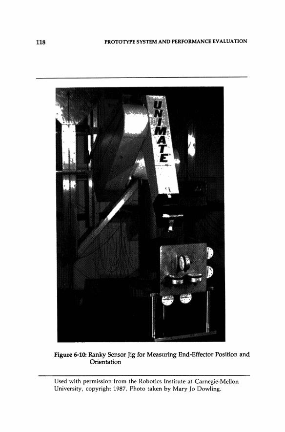
118 PROTOTYPE SYSTEM AND PERFORMANCE EVALUATION
Figure 6-10: Ranky Sensor Jig for Measuring End-Effector Position and Orientation
Used with permission from the Robotics Institute at Carnegie-Mellon University, copyright 1987. Photo taken by Mary Jo Dowling.

PROTOTYPE SYSTEM AND PERFORMANCE EVALUATION 119
indicated in Figure 6-10. A similar box comer, made of an aluminum alloy,
is affixed to the end-effector. It too has an associated coordinate frame im
plicit to its shape. The objective is to place the cube on the end-effector into
the jig so as to deflect the nine dial gauges. From the measured deflections
and the known placement of the gauges, one can determine the position and
orientation of the end-effector relative to the sensor jig.
We mounted the sensor jig on the bed of a three-axis milling machine
equipped with linear optical encoders. The jig can thus be displaced ac
curately over a large volume. A set of approach points are defined to insure
that the test cube does not damage the dial gauge stems by hitting them
sideways. In addition, the retraction of the test cube from the jig permits
indexing of the machine bed. The robot is programmed to first position the
end-effector at an approach point. At a reduced speed, the end-effector then
moves to the corresponding vertex point, deflecting the nine dial gauges.
The end-effector remains at the vertex point while the dial gauges are read
and the measurements are recorded. The end-effector then returns to the
approach point and the sensor jig is translated to the next vertex point. The
speed is temporarily increased during motions between successive approach
points. The dial gauges have a resolution of 0.001 in. The accuracy of our
sensor jig is 0.001 in. in position and 0.01 degree in orientation. In the
experimental results which follow, the grid size was 25 cm x 25 cm x 60 cm.
The measured set of dial gauge deflections are uploaded to the VAX 11/780
and stored. Separate software, residing on the VAX 11/780, processes the
grid touching measurement data and tabulates indices of kinematic perfor
mance. Grid line perpendicularity, line straightness, and line length are the
primary features of interest.
The three-dimensional grid touching experiments were conducted in
the Civil Engineering Department Machine Shop at Carnegie-Mellon Univer-
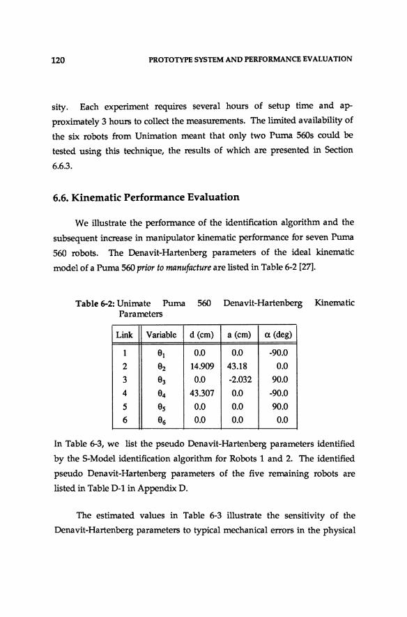
120 PROTOTYPE SYSTEM AND PERFORMANCE EV ALUA nON
sity. Each experiment requires several hours of setup time and ap
proximately 3 hours to collect the measurements. The limited availability of
the six robots from Unimation meant that only two Puma 560s could be
tested using this technique, the results of which are presented in Section
6.6.3.
6.6. Kinematic Performance Evaluation
We illustrate the performance of the identification algorithm and the
subsequent increase in manipulator kinematic performance for seven Puma
560 robots. The Denavit-Hartenberg parameters of the ideal kinematic
model of a Puma 560 prior to manufacture are listed in Table 6-2 [27].
Table 6-2: Unimate Puma 560 Denavit-Hartenberg Kinematic Parameters
Link Variable d (cm) a (cm) a (deg)
I 91 0.0 0.0 -90.0 2 92 14.909 43.18 0.0 3 93 0.0 -2.032 90.0 4 94 43.307 0.0 -90.0 5 9s 0.0 0.0 90.0 6 96 0.0 0.0 0.0
In Table 6-3, we list the pseudo Denavit-Hartenberg parameters identified
by the S-Model identification algorithm for Robots 1 and 2. The identified
pseudo Denavit-Hartenberg parameters of the five remaining robots are
listed in Table D-1 in Appendix D.
The estimated values in Table 6-3 illustrate the sensitivity of the
Denavit-Hartenberg parameters to typical mechanical errors in the physical

PROTOTYPE SYSTEM AND PERFORMANCE EVALUATION 121
Table 6-3: Identified Arm Signature Parameters
Name Link Variable 9o//set (deg) d (em) a (em) ex (deg)
1 91 110.308 -20.678 -0.005 -90.066
2 92 79.977 11,210.213 7.607 -0.217
3 93 -79.483 -11,194.978 -2.039 90.519 Robot 1
4 94 -0.296 43.278 -0.001 -90.007
5 9s -0.497 -0.018 0.002 89.990
6 96 -89.081 10.300 0.000 0.000
1 91 110.849 -20.428 -0.023 -90.013
2 92 63.467 2,783.580 19.084 -0.803
3 93 -63.276 -2,768.574 -2.028 90.134 Robot 2
4 94 0.328 43.299 -0.009 -89.991
5 8s -0.126 -0.054 0.007 89.969
6 86 -89.517 10.273 0.000 0.000
manipulator. For instance, the values of ~ and d3 in Table 6-3 indicate that
the joint 2 and joint 3 axes are slightly out of parallel. Customarily, this is
referred to as the convergence angle problem. When these axes are slightly out
of parallel, their common normal lies extremely far from the physical
manipulator (refer to Figure 2-2). Since the origin of the Denavit-Hartenberg
Link 2 coordinate frame is defined by the intersection of the joint 2 axis and
this common normal, it too lies extremely far from the physical manipulator.
The parameters d2 and ~, which are opposite in sign and nearly equal in
magnitude, represent the translation out to and back from the link 2 coor
dinate frame, respectively. The dramatic differences between the identified
and the ideal parameters arise from small manufacturing errors.
The error committed in positioning and orienting the robot end
effector is a measure of the cumulative accuracy of the kinematic parameters

122 PROTOTYPE SYSTEM AND PERFORMANCE EVALUATION
upon which the control algorithms are based. For the parameters identified
in Table 6-3, the cumulative accuracy can also be measured by determining
the mean square errors between the Cartesian target positions and the iden
tified features. Intuitively, as the overall accuracy of the identified signature
increases these errors decrease.
In Section 4.3.2.1, our estimate of a plane-of-rotation feature minimizes
the sum of the squares of the perpendicular errors between the target posi
tions and the plane. Similarly, in Section 4.3.2.2, our estimate of a circle of
rotation minimizes the sum of the squares of the perpendicular errors be
tween the projected target positions and the circle. The algorithms presented
in Sections 4.3.2.1 and 4.3.2.2, for minimizing these functions, are implicitly
based upon the assumption that the measurement errors (i.e., the residual
errors) are random and normally distributed. In Figure 6-11, we have
plotted the residual errors in fitting a plane and a circle to the measured
Cartesian positions of Target Point 6 corresponding to the identified sig
nature of Robot 1 listed in Table 6-3. The perpendicular errors between the
target's positions and the identified plane (i.e., the normal residuals) are
indicated by asterisks. The circles represent the perpendicular errors be
tween the projected target positions and the identified circle (i.e, the radial
residuals). These errors are plotted as a function of the measurement num
ber. (The measurement number corresponds to the index i in Figure 4-1.)
The behavior of the residuals in Figure 6-11, as a function of the measure
ment number, is typical of the behavior of the residuals which correspond to
the remaining identified signatures in Table D-1. The lack of any significant
systematic trends in the normal and radial residuals leads us to assume that
the target position errors are random. Furthermore, we have observed that
the distributions of the residual errors are closely approximated by the nor
mal distribution. To illustrate, Figures 6-12 and 6-13 contain the histograms
of the twelve sets of residual errors corresponding to the identified arm

PROTOTYPE SYSTEM AND PERFORMANCE EVALUATION
E' 0.04 ~
~ ~ 0.03
~ 0.02
0.01
-0.02
-0.03
-0.04
Normal Residuals
Radial Residuals
123
Measurement Number
Figure 6-11: Residuals: Normal to Plane and Radial (Joint 6)
signature of Robot 1. The sample variances and standard deviations of these
residuals are listed in Table 6-4.
The essential aspect of a plane-of-rotation is its angular orientation.
The accuracy of the angular orientation of an identified plane-of-rotation is a
function of the accuracy of the target measurements, the number of measure
ments Nj , and the nominal radius of the target point. In Section 4.3.2.1, we
applied simple linear regression techniques to estimate the parameters E, F,
and G in (4.19) which define the identified plane-of-rotation. The physical
interpretation of these parameters is illustrated in Figure 6-14. It is noted that

124 PROTOTYPE SYSTEM AND PERFORMANCE EVALUA nON
30 r 1 Joint 1 5 I Joint 2
~ .. !
~ ~ ~ Ii;;
5
35 ~ Joint 4 30
j 25
Joint 3
5
0
5
-D.5 0.2 0.4 ReBidUldIl (mm)
~
! Joint 5 Joint 6
5
0
Figure 6-12: Histogram Plots of the Residuals for the Plane-of-Rotation Estimates for Joints 1 through 6

PROTOTYPE SYSTEM AND PERFORMANCE EVALUATION 125
I 25 I I Joint 1 Joint 2
5 5
0 0
5
~.I 0.1
~ ~ 35
f Joint 3 f Joint 4 u; u;
5
0
5
~ ~
l or: Joint 5 ~ Joint 6 1
Figure 6-13: Histogram Plots of the Residuals for the Circle-of-Rotation Estimates for Joints 1 through 6

126 PROTOTYPE SYSTEM AND PERFORMANCE EV ALUA TION
Table 6-4: Sample Variances and Standard Deviations of the Normal and Radial Residuals
Nonnal Residuals Radial Residuals Joint Variance Stdev Variance Stdev
(cm 2) (cm) (cm 2) (cm)
1 0.000187 0.0137 0.000133 O.oI15
2 0.000848 0.0291 0.000329 0.0181
3 0.001437 0.0379 0.000202 0.0142
4 0.000114 0.0107 0.000416 0.0204
5 0.000142 0.0119 0.000090 0.0095
6 0.000230 0.0152 0.000230 0.0152
z
y
x
Figure 6-14: An Identified Plane-of-Rotation
during the final iteration of the repeated least-squares algorithm, the es
timated parameters E and F, in the model (4.19), will be approximately zero.
If the residual errors ~j , in (4.22), are independent with zero mean and

PROTOTYPE SYSTEM AND PERFORMANCE EVALUATION 127
variance O'~, then the estimate e (4.23) will be unbiased [29]. Furthermore,
the variance of e will be
(6.8)
where ~ is defined in (4.24). Expanding (6.8) yields n
O'~LY'J VAR(E)
2 j=l - O'E = n n n (6.9)
LX'~LY'~ - [LX'Y']2 . 1 J. 1 J and J= J= j=l
n
O'~LX'J VAR(F) 2 j=l
- O'F = n n n
:L,X'~:L,Y'~ - [:L,£'Y']2 . 1 J. 1 J
J= J= j=l
(6.10)
where X'j and Y'j represent the original Xj and Yj minus their respective means
(i.e., X'j=xrx andY'j=YrY). The estimated variances ofE and F are computed
according to (6.9) and (6.10) with O'~ replaced by the sample variance of the
normal residuals.
A variation in the parameter E corresponds to an angular variation in
the slope of the plane parallel with the X axis. Similarly, a variation in the
parameter F corresponds to an angular variation in the slope of the plane
parallel with the Y axis. When the parameters E and F are small (i.e., much
less than 1.0) and their variances are also small, the variances (6.9) and (6.10)
represent the variances of the angular orientation of the plane with respect to
the X and Y axes, expressed in units of rad 2• The standard deviations of the
estimates E and F, O'E and O'F' provide a physically meaningful measure of
the orientational accuracy of the estimated plane-of-rotation. These standard
deviations translate into confidence intervals which can be compared with

128 PROTOTYPE SYSTEM AND PERFORMANCE EVALUATION
manufacturing tolerances to determine whether an identified signature is
likely to be more or less accurate than the robot's design model. If the
standard deviation in the orientational accuracy of the planes-of-rotation are
significantly greater than the orientational accuracy with which the robot can
be manufactured, then it is highly probable that the identified signature will
actually degrade the performance of the robot.
For many robots, the expressions (6.9) and (6.10) can be simplified due
to the symmetry of the target measurements in the X-Y plane. For instance,
consider a joint which has 360 degrees of rotation. The X and Y coordinates
of the target's positions, with respect to the coordinate frame indicated in
Figure 6-14, lie essentially on a circle of radius R i • According to the
methodology outlined in Section 4.3.2.1, these points are equally spaced
along the circle's circumference. Consequently, the covariance of the X and
Y coordinates of the measurements is zero. Therefore, the term 41 ~j9'j in
(6.9) and (6.10), equals zero. Furthermore, it can be readily shown that the
sums Lj:1~; and 4=19'; are equal to nR2i /2.0. The variance in the angular
orientation of the plane is, in this case, the same in all directions and equal to
2 Rin
(6.11)
We are thus 95 percent confident that the true angular orientation of the
plane lies within ± 2o'lj radians of the estimated orientation. The expression
(6.11) for the variance is intuitively pleasing. As the accuracy of the
measurements decrease the accuracy of the estimate decreases; as the
nominal radius of the increases the accuracy of the estimate increases; and as
the number of measurements increases the accuracy of the estimate in
creases. Most importantly, The expression (6.11) provides a simple
mechanism for determining how to select the identification parameters nand

PROTOTYPE SYSTEM AND PERFORMANCE EVALUATION 129
Ri given the accuracy of a proposed sensor system and the manufacturing
tolerances of the robot.
In general, for a joint with less than 360 degrees of rotation, the
variance in the angular orientation of the estimated plane-of-rotation varies
with the direction within the plane. The maximum occurs in the direction in
which the projection of the measurements onto the plane has the least
variance. If, for instance, the minimum and maximum limits on the motion
of a joint are 0 degrees and 270 degrees, respectively, then the maximum
variance in angular orientation of the estimated plane-of-rotation will occur
in the direction of 315 degrees. The exact value for the maximum variance
can be computed using (6.9). However, for joints with at least 180 degrees of
rotation, we have determined experimentally that the maximum variance is
closely approximated by
2 2 an
as '" (6.12) 2 R j n (.OO244X - .344)
where X represents the joint range of motion in degrees. The expression
(6.12) is a conservative approximation.
Table 6-5 lists the variances and standard deviations of the angular
orientation of the identified planes-of-rotation corresponding to the iden
tified arm signature of Robot 1, listed in Table 6-3. For Joint 6, the orien
tation of the identified plane-of-rotation is accurate to within ±.0074deg.
Similar results are obtained for the remaining signatures listed in Table D-l.
It is apparent that the orienta tiona I accuracies of the identified planes-of
rotation are significantly greater than the machining and assembly accuracies
with which commercially available robots are manufactured. Such ac
curacies may be on the order of hundredths of a degree or more.

130 PROTOTYPE SYSTEM AND PERFORMANCE EV ALUA nON
Table 6-5: Orientational and Positional Accuracy of the Identified Planes-of-Rotation and Centers-of-Rotation Corresponding to the Arm Signature of Robot 1
Feature Estimate Accuracy Joint Plane-of-Rotation Center -of-Rotation
0"1) (deg) O"c(cm)
1 .002937 .00176
2 .007397 .00335
3 .008514 .00250
4 .003204 .00356
5 .004149 .00184
6 .003699 .00176
The essential aspect of a center-of-rotation is its position relative to a
joint axis. The accuracy of the position of an identified center-of-rotation is a
function of the accuracy of the target positions measured relative the joint
axis. Since the origin of an S-Modellink coordinate frame is permitted to lie
anywhere on the joint axis, errors in the identified position of a center-of
rotation in the direction of the joint axis, have no effect upon the accuracy of
the identified kinematic parameters. In Section 4.3.2.2, we applied simple
linear regression techniques to estimate the parameters A, B, and C which
define the identified circle-of-rotation. The parameters A and B are linearly
related to the X and Y coordinates of the center-of-rotation. Unfortunately,
since the errors in measuring w (4.37), are dependent upon x and y, a deriva
tion of the variances of the estimates of the parameters A and B analogous to
that for the parameters E and F is impossible.
We have applied Monte-Carlo simulation techniques to empirically

PROTOTYPE SYSTEM AND PERFORMANCE EVALUATION 131
determine the relationship between the variance in the estimated coordinates
of the center-of-rotation, the variance in the measurements, the range of mo
tion of the joint, and the number of measurements. In these simulations, we
have assumed that the errors in the measurements of the target point coor
dinates, Xj and Yj , are independent and normally distributed with zero mean
and variance a2 I(2x2)' Furthermore, it is assumed that the target radius is
much larger than the measurement noise, as would be the case in practice.
The simulation experiments demonstrate that the radial residuals (i.e., the
errors in w) are essentially characterized by a normal distribution. For joints
with 360 degrees of rotation, the variances in the estimated coordinates of the
center-of-rotation are equal while for joints with less than 360 degrees of
rotation, these variances will differ. For our purposes, we characterize the
accuracy of the coordinates of the estimated center-of-rotation by the max
imum variance, denoted by 0';. The relationship between the variance 0';, the
number of measurements, and the range of motion of the joint is found to be
2 2 O'r
0' c ... -n"""( .'""00""2:"::2':'9 X=---.'""3"""13~) , (6.13)
where a; is the variance of the radial residuals and X is the range of motion
of the joint measured in degrees. The accuracy of an estimated center-of
rotation can be increased by either increasing the accuracy of the sensor
system or increasing the number of measurements.
Table 6-5 lists the positional accuracies of the identified centers-of
rotation for the arm signature of Robot 1. The positional accuracy of the
identified Joint 6 center-of-rotation is ±O.OO176 cm. Again, this exceeds the
machining tolerances with which commercially available robots are
manufactured. The accuracies of the identified features of Robots 2 through
7 are essentially the same as those for Robot 1. In the following sections, we

132 PROTOTYPE SYSTEM AND PERFORMANCE EV ALUA nON
demonstrate that the identified ann signatures of Robots 1 through 7 are
indeed more accurate than the design model by applying them to improve
the kinematic performance of all seven robots.
6.6.1. One-Dimensional Performance Evaluation
We have applied the one-dimensional grid touching task to evaluate
the kinematic performance of Robot 1, both with and without arm signature
identification. Table 6-6 lists a sampling of results obtained in this task.
Table 6-6: Line Length Errors
Desired Design Model Signature Model
Line Length
(em) Length Error Length Error
(em) (em) (em) (em)
1 60.0 59.470 -0.530 59.959 -0.050
2 50.0 50.350 0.350 49.875 -0.125
3 60.0 59.710 -0.290 59.940 -0.060
4 50.0 60.325 0.325 49.895 -0.105
5 60.0 59.375 -0.625 59.960 -0.040
6 60.0 59.725 -0.275 59.955 -0.045
Lines 1 and 4 are nominally aligned with the robot's X axis; Lines 2 and 5 are
nominally aligned with the robot's Y axis; and Lines 3 and 6 are nominally
aligned with the robot's Z axis. The locations of Lines 1 through 6, relative to
the base of the robot, are depicted in Figure 6-15. The approximate coor
dinates of the Lines 1 through 6 are listed in Table 6-7. (Note that the X-V
plane of the base coordinate frame indicated in Figure 6-15 is coincident with
the surface of the table to which the robot is mounted. Fonnally, the X-V
plane of the base coordinate frame is parallel with the Joint 2 axis.)

PROTOTYPE SYSTEM AND PERFORMANCE EVALUATION 133
Figure 6-15: Approximate Location of Lines 1 through 6
Table 6-7: Line Coordinates Measured Relative to Base Coordinate Frame
Line X Coordinate Y Coordinate Z Coordinate
(em) (em) (em)
1 - 58.0 3.0
2 8.0 - 38.0
3 8.0 73.0 -4 - 8.0 38.0
5 -58.0 - 3.0
6 -73.0 8.0 -
The results listed. in Table 6-6 indicate that the identified arm signature
134 PROTOTYPE SYSTEM AND PERFORMANCE EV ALUA nON
model significantly improves the Cartesian displacement accuracy of the
Puma 560. Similar results have been obtained throughout the robot's
workspace. From these results, we can further illustrate that the arm sig
nature model is cumulatively more accurate than the design model.
If we assume that the design model accurately represents the kinematic
structure of Robot 1, we can apply it to predict the displacement error
generated by using the signature model for control. For instance, consider
Line 1. According to the signature model, the desired Cartesian position and
orientation of the end-effector at the beginning and end of the line cor
respond to the two joint configurations
711=[-48.062 -200.056 56.300 0.241 -36.208 41.812]T
and
712=[-102.706 -199.448 54.660 1.880 -35.392 -14.207f ,
respectively. Using the design model, configurations 711 and 712 correspond
to the two Cartesian end-effector positions (-32.047, 57.957, -56.562) and
(28.519,59.118, -56.555), respectively. The predicted displacement of the end
effector is thus 60.577 cm and the predicted displacement error is 0.577 cm.
This compares with the actual measured displacement error of -0.050 cm. On
the other hand, if we assume that the signature model accurately represents
the kinematic structure of Robot 1, we can apply it to predict the displace
ment error generated by using the design model for control. According to
the design model, the desired Cartesian position and orientation of the end
effector at the beginning and end of the line corresponds to the two joint
configura tions
71 1 = [-48.106 -200.029 56.287 0.0 -36.258 41.894]T
and
712=[-102.385 -197.951 50.4860.0 -32.534 -12.385]T ,
PROTOTYPE SYSTEM AND PERFORMANCE EVALUATION 135
respectively. Using the signature model, configurations 7/1 and 7/2 cor
respond to the two Cartesian end-effector positions (-31.019, 57.813, -57.300)
and (28.394, 57.065, -57.245), respectively. The predicted displacement of the
end-effector is thus 59.418 cm and the predicted displacement error is -0.582
em. This error compares with the actual measured displacement error of
-0.530 em. In this case and others, the signature model is clearly a better
predictor of displacement errors than the design model. Therefore, the sig
nature model is cumulatively more accurate than the design model.
6.6.2. Two-Dimensional Performance Evaluation
We have applied the two-dimensional grid touching task to evaluate
the kinematic performance of Robots 2 through 7. Figure 6-16 illustrates the
position and orientation of the grid relative to the robot's base as viewed
from above the table. The X and Y axes of the grid were nominally aligned
with the X and Y axes of the robot's base coordinate frame. The grid spans
60 cm in the X direction and 15 em in the Y direction. The grid contains 62
uniformly spaced points (i.e., vertices). The desired X and Y axis spacings
were both 5.0 cm.
The features used to measure the performance of a robot are line
length, line straightness and grid perpendicularity. Ideally, the end
effector's position would have coincided with the intersection points of Lines
Xl,X2,X3,X4 and Lines Yl,n, ... ,Y13, indicated in Figure 6-16. In reality,
the grid lines are neither parallel, perpendicular, nor straight. We denote the
actual grid lines by Xl·,X2·,X3·,X4· and Yl.,n·, ... ,Y13. The line xi" is
defined to be the line which passes through the actual recorded points (l,i)
and (l3,i). Similarly, the line Y/ is defined to be the line which passes
through the actual recorded points G,1) and (j,4). The actual length of line xi" is the distance between points (l,i) and (l3,i). The actual length of line Y/ is

136 PROTOTYPE SYSTEM AND PERFORMANCE EVALUATION
• Indicates Vertex
Point
Base
Xl X2 X3 X4
Yl Y2 Y3 Y4 YS Y6 Y7 Y8 Y9 YlO Yll Yl2 Y13
Figure 6-16: Relative Location of Two-Dimensional Grid
the distance between points (j,l) and (j,4). For each line, we also measure the
normal deviation of the intermediate points. The maximum normal devia
tion provides a measure of the straightness (i.e., the curvature) of the grid
line. The perpendicularity of the grid is determined by measuring the length
of the grid diagonals (i.e., the distances between actual points (1,1) and (13,
4), and points (13,1) and (1,4».
Tables 6-8 and 6-9 are a summary of the results obtained in the two
dimensional grid touching task. Table 6-8 pertains to the case where the
design model is applied to control the position and orientation of the end
effector and Table 6-9 pertains to the case where the signature model is
applied to the control the end-effector. The columns labeled X Line Length
Error and Y Line Length Error represent the maximum deviation in line length

PROTOTYPE SYSTEM AND PERFORMANCE EVALUATION 137
Table 6-8: Two-Dimensional Grid Touching Task Performance Summary Using the Design Model
X Line YLine Maximum Diagonal 1 Diagonal 2
Robot Length Length Normal Length Length Error Error Deviation Error Error
1
2
3
4
5
6
(em) (em) (em) (em) (em)
0.100 -0.575 0.150 -0.495 -0.320
0.075 -0.150 0.050 -0.170 -0.070
0.150 0.300 0.075 0.480 0.105
0.050 -0.750 0.025 -0.095 0.005
-0.075 0.350 0.075 -0.695 0.230
-0.125 0.950 0.125 0.755 0.705
Table 6-9: Two-Dimensional Grid Touching Task Performance Summary Using the Signature Model
X Line YLine Maximum Diagonal 1 Diagonal 2
Robot Length Length Normal Length Length Error Error Deviation Error Error (em) (em) (em) (em) (em)
1 -0.050 -0.050 0.025 -0.020 0.005
2 0.050 -0.050 - 0.030 -0.095
3 0.075 0.075 0.025 0.105 0.030 4 0.075 -0.025 - -0.080 -0.095
5 0.050 -0.100 - -0.045 -0.070
6 -0.025 0.050 0.025 0.030 0.105
among the sets of lines Xl·,Xt,X3·,X4· and Yl·,n·, ... ,Y13·, respectively.
The column labeled Maximum Normal Deviation represents the maximum of
the set of 4 maximum normal deviations for lines Xl·,X2·,X3·,X4·. (Since the
lines Yl·, n", ... ,Y13· are only 15 cm long, the observed normal deviations
are negligible.)

138 PROTOTYPE SYSTEM AND PERFORMANCE EVALUATION
A comparison of the results in Table 6-8 with the results in Table 6-9
again indicates that use of the identified signature model to control the end
effector's Cartesian position and orientation leads to a general improvement
in the kinematic performance of all 6 robots. Unfortunately, due to the
limited accuracy with which these specific measurements were obtained, it is
difficult to state with any accuracy by what factor the performance has in
creased.
6.6.3. Three-Dimensional Performance Evaluation
We have applied the three-dimensional grid touching task to evaluate
the kinematic performance of Robots 3 and 5. The X and Y axes of the grid
were nominally aligned with the X, Y, and Z axes of the robot's base coor
dinate frame. The grid spans 60 cm in the X direction, 25 cm in the Y
direction, and 25 cm in the Z direction. The range in the Y and Z directions
was limited by the throw of the corresponding two axes of the milling
machine. The grid contains 63 uniformly spaced points (i.e., vertices). The
desired X, Y, and Z axis spacings were 10.0 em, 12.5 cm, and 12.5 em, respec
tively.
The features used to measure the performance of a robot are line
length, line straightness, grid line perpendicularity, radial deviation, and
orientational deviation. In analogy to the two-dimensional grid, the three
dimensional grid contains 9 lines nominally parallel with the X axis, 21 lines
nominally parallel with the Y axis, and 21 lines nominally parallel with the Z
axis. The actual lines are defined by the corresponding pairs of points along
the grid's border. In Tables 6-10 and 6-11, we summarize thirteen measured
indices which describe the relative improvements in the kinematic perfor
mance of Robots 3 and 5, respectively. The last column in each of these tables
lists the performance improvement factor which is the ratio of the error

PROTOTYPE SYSTEM AND PERFORMANCE EV ALUA nON 139
Table 6-10: Three-Dimensional Grid Touching Task Performance Summary for Robot 3
Description Design Signature Improvement Model Model Factor
Maximum Normal Deviation from a Line 0.071 0.023 3.09
Parallel with the X Axis
Maximum Normal Deviation from a Line 0.023 0.006 3.83
Parallel with the Y Axis
Maximum Normal Deviation from a Line 0.019 0.007 2.71
Parallel with the Z Axis
Magnitude of Line Length Error for 0.055 0.077 0.71
Line Parallel with the X Axis
Magnitude of Line Length Error for 0.096 0.016 6.00
Line Parallel with the Y Axis
Magnitude of Line Length Error for 0.027 0.013 2.08 Line Parallel with the Z Axis
Deviation from Perpendicular between -1.040 -0.096 10.83 X Axis and Y Axis Grid Lines
Deviation from Perpendicular between -0.278 0.229 1.21 Y Axis and Z Axis Grid Lines
Deviation from Perpendicular between -0.505 -0.238 2.12
Z Axis and X Axis Grid Lines
Relative Orientational Deviation about 0.153 -0.038 4.00 X Axis at Vertex 4
Relative Orientational Deviation about -0.157 0.038 4.14 Y Axis at Vertex 4
Relative Orientational Deviation about -0.067 -0.027 2.50 Z Axis at Vertex 4
committed when the arm signature model is used for control to the error

140 PROTOTYPE SYSTEM AND PERFORMANCE EV ALUA nON
Table 6-11: Three-Dimensional Grid Touching Task Performance Summary for Robot 5
Description Design Signature Improvement Model Model Factor
Maximum Normal Deviation from a Line 0.066 0.023 2.87
Parallel with the X Axis
Maximum Normal Deviation from a Line 0.022 0.006 3.67
Parallel with the Y Axis
Maximum Normal Deviation from a Line 0.038 0.009 3.98
Parallel with the Z Axis
Magnitude of Line Length Error for 0.139 0.182 0.76
Line Parallel with the X Axis
Magnitude of Line Length Error for 0.110 0.016 6.88
Line Parallel with the Y Axis
Magnitude of Line Length Error for 0.079 0.026 3.04
Line Parallel with the Z Axis
Deviation from Perpendicular between -0.974 -0.077 12.65
X Axis and Y Axis Grid Lines
Deviation from Perpendicular between 0.365 0.226 1.62
Y Axis and Z Axis Grid Lines
Deviation from Perpendicular between 0.271 -0.160 1.69
Z Axis and X Axis Grid Lines
Relative Orientational Deviation about 0.172 0.000 -X Axis
Relative Orientational Deviation about -0.086 -0.005 16.0
Y Axis
Relative Orientational Deviation about -0.041 -0.014 3.01
Z Axis
committed when the design model is used for control. The improvement
factors range between 0.71 and 16.0.

PROTOTYPE SYSTEM AND PERFORMANCE EVALUATION 141
6.7. Conclusions
In this chapter, we have described our hardware/software implemen
tation of a complete prototype arm signature identification system and have
applied this system to improve the positioning accuracy of seven Puma 560
robots. This system incorporates an ultrasonic range sensor to measure the
three-dimensional Cartesian positions of target sparkers placed on the
rooot's links. The S-Model identification algorithm uses the target position
measurements to first identify a set of robot kinematic features and then
combines the information contained therein to identify the robot's Denavit
Hartenberg kinematic parameters. This algorithm leads to an efficient
method for collecting measurements. Using our prototype system,
thousands of measurements can be obtained in less than one hour. The use
of our prototype system to increase the performance of actual robots
demonstrates that the S-Model identification algorithm is both feasible and
practical.
A key issue in the design of an arm signature identification system is
the selection and/or design of a sensor system. Our sensor system incor
porates a commercially available ultrasonic range sensor to measure the
three-dimensional Cartesian positions of target sparkers placed on the
robot's links. A unique sensor array design and specialized slant range
compensation algorithms are used to obtain ultrasonic range measurements
which are significantly more accurate (by a factor of 10-50) than accuracies
which can be obtained using the commerCially available system itself.
For arm signature identification, the ad van tages of using our ultrasonic
sensor system design are:
• The sensor array can be easily calibrated.

142 PROTOTYPE SYSTEM AND PERFORMANCE EV ALUA TION
• The fixtures required to attach the target sparkers to the robot are extremely simple to manufacture and there placement with respect to the links is essentially arbitrary. This avoids the need for elaborate and costly fixturing.
• The sensor system can be easily interfaced to a host computer (typically the robot controller) which can coordinate the digitizing operation while simultaneously controlling the robots motions.
• The ultrasonic emission characteristics of the sparkers are such that they can be modeled as infinitely small point sources. The sparkers are thus ideally suited for implementing the target points used in the 5-Model identification algorithm.
• The sparkers and the microphones remain stationary during the measurement process. This is, for instance, in contrast to optical devices which would customarily require an elaborate positioning system to enable the detector to track and locate the position of a target. A voiding the tracking problem leads to a simple, efficient, and relatively inexpensive sensor system.
• The sensor system has a large dynamic range with high resolution. The active volume is a cube approximately 1.5 meters in length and the Cartesian positioning accuracy is on the order of ± 0.02 em.
• The speed at which range measurements can be acquired and the Cartesian positions of the target can be determined enables high sampling rates (on the order of 4 measurements/sec) to be achieved.
• The configuration of the sensor array and the two calibration rods are fixed and independent of the target sparker. Thus, the measurements for identifying the arm signatures of a variety of robots can be obtained without reconfiguring or recalibrating the sensor array.
• Remote range sensing eliminates the need to position detectors within close proximity to the target and avoids the problems associated with contact sensing.
• The ability to increase the target radii provides a mechanism for increasing arm signature accuracy.

PROTOTYPE SYSTEM AND PERFORMANCE EV ALUA TION
• The operation of the sensor system can be completely automated thus eliminating the need for a highly skilled operator.
143
We have devised three methods for evaluating manipulator kinematic
performance in which the Puma is programmed to position its end-effector
at the vertices of a one-, two-, or three-dimensional grid. At each of the grid
vertices, the actual relative position of the end-effector is measured.
In the one-dimensional grid touching task, the relative position of the
end-effector is measured with a cathetometer. The tip of a pin, attached to
the end-effector is sighted through the telescope of the cathetometer. The
task is performed twice, once using signature based control and once using
the design kinematic model for control. The relative improvement in perfor
mance is then determined. With signature-based control, the end-effector
positioning accuracy of one Puma 560 robot was increased by as much as a
factor of 10.0. The lowest increase in performance for this same robot was a
factor 2.8.
In the two-dimensional grid touching task, the workspace coordinate
frame is aligned with the surface of a table and a custom-designed, spring
loaded pen is attached to the robot's end-effector. The positions of the end
effector are recorded when the pen touches the mylar surface. A machinist's
rule is applied to measure the relative positional deviations in the grid
points. Features of interest are the perpendicularity of the lines defined by
the vertices, line straightness, and line length. The measured performance of
six Puma 560 robots using design model based control and signature-based
control are listed in Tables 6-8 and 6-9, respectively. These tables describe
the general improvement in the performance of all six robots.
In the three-dimensional grid touching task, a jig is mounted on the
table of a three-axis milling machine. As the robot approaches a desired

144 PROTOTYPE SYSTEM AND PERFORMANCE EVALUATION
target point, the precision test cube attached to its end-effector deflects the
nine dial gauges within the jig. The relative Cartesian position and orien
tation of the end-effector is computed based upon the measured deflections
and the known geometry of the gauge array. The three instrumented axes of
the milling machine are used to accurately position the jig in three dimen
sions. The robot is programmed to position its end-effector at 63 vertex
points within a rectangular grid coinciding with the position of the jig. This
technique has been applied to measure and evaluate the performance of two
Puma 560 robots, the results of which are listed in Tables 6-10 and 6-11. As
in the previous two methods, the performance of these robots was sig
nificantly increased by using the identified kinematic parameters for control.
The performance improvement factors listed in Tables 6-10 and 6-11 range
between 1.21 and 16.0, with but two exceptions.
The improvements are not as large as one might expect based upon the
feature estimate accuracy predictions listed in Table 6-5. The disparity is
believed to be caused by the presence of small biases in the individual range
measurements, and this appears to be the limiting factor in the performance
of our prototype system. In order to obtain additional improvements in
manipulator kinematic performance, alternative sensor systems may be
necessary.

Chapter 7
Performance Evaluation Based Upon Simulation
7.1. Overview
In this chapter, we consider the statistical performance of robot posi
tion control methods, and discuss the origin of robot positioning errors. In
conventional design-model robot control, the robot design model is used as a
basis for kinematic control. In this case, manufacturing errors contribute
most to robot positioning errors. In arm signature-based robot control (5-
Model), the correct arm signature model eliminates kinematic errors due to
manufacturing. In this case, robot performance is limited by sensor errors
which contribute to inaccuracy of the identified arm Signature model.
Experimental studies of D-Model and S-Model control were described
in the previous chapter. In those studies, the S-Model control showed con
sistent performance improvement, and demonstrated accuracy approaching
limits predicted by the joint encoder resolution. In this chapter, we analyze
the origin of this improvement, and quantify the requirements of an arm
signature identification system in terms of the underlying sensor perfor
mance.
D-Model control performance depends upon the manufacturing
process which determines the actual geometry of the robot. Since manufac
turing error vary randomly from one robot to another, the performance of an
146 PERFORMANCE EV ALUA TlON BASED UPON SIMULATION
arbitrarily chosen robot has a random component. The statistical parameters
which characterize a robot's positioning accuracy are related to the statistical
parameters which characterize the manufacturing error probability distribu
tion functions. Unfortunately, the complexity of robot kinematics prevents
us from analytically deriving this relationship.
In this chapter, we apply Monte-Carlo simulation techniques to gain
insight into the relationship between manufacturing error and the perfor
mance of a design model controller. A kinematic model of a Puma 560 robot
which directly incorporates manufacturing errors as parameters has been
developed for our analysiS and is described in Section 7.2.2. The results of
our analysis are presented in Section 7.4.1 and 7.4.2, and bring to light some
of the major disadvantages of the design model control approach.
The performance of S-Model control is dictated by the presence of er
rors in the arm signature identification process and not by the presence of
manufacturing errors. Errors are introduced into the identification process
by the sensor system and must be analyzed to determine if the performance
of the robot is improved relative to the performance obtained by Controller
D. In this chapter, we analyze the relationship between target measurement
errors and Controller 5 performance using simulation tpethods.
This chapter is organized as follows. In Section 7.2, we describe the
structure of our Monte-Carlo simulator and test its validity in Section 7.3.
Then, in Sections 7.4.1 and 7.4.2, we explore the relationship between the
performance of the D-Model controller and the two types of manufacturing
errors referred to as encoder calibration errors and machining and assembly
errors. Sections 7.4.3 - 7.4.5 discuss the relationships between the perfor
mance of the S-Model controller and the target measurement accuracy, the
number of measurements, and the length of the target radii, respectively.

PERFORMANCE EVALUATION BASED UPON SIMULA nON 147
Finally, in Section 7.5, the issue as to whether or not S-Model control im
proves robot end-effector positioning accuracy is resolved.
7.2. A Monte-Carlo Simulator
In this section, we describe a Monte-Carlo simulation of a robot under
either D-control or S-control and analyze the effects of the various error
sources on resulting perfonnance.
The performance evaluation of these two controllers is complicated by
the nonlinear robot kinematics, the nonlinearities of the S-Model identifica
tion algorithm, and the presence of error sources. Random errors are intro
duced into both the manufacturing and identification processes. This reality
forces us to develop a Monte-Carlo simulator to conduct a statistical evalua
tion. Because of the variability of robot designs, development of a general
purpose Monte-Carlo simulator was impractical. Thus, to complement our
hardware experimentation, we have evaluated the kinematic performance of
the Puma 560 robot with both design model based control and signature
based control. In doing so, we have established a methodology to evaluate
the kinematic perfonnance of all robots.
7.2.1. Evaluating Kinematic Performance
The three-dimensional grid touching task is used in simulation to
evaluate the kinematic perfonnance of the Puma 560 with alternative con
troller designs. The grid contains twelve vertices, labeled 1 through 12,
whose approximate positions, relative to the robot, are indicated in Figure
7-1. The desired positions of the vertices, measured with respect to the base
coordinates of an ideal Puma 560 are listed in Table 7-1. The desired orien
tation of the end-effector is the same for all twelve vertices. The orientational

148 PERFORMANCE EVALUA nON BASED UPON SIMULATION
Robot Base Coordinate Frame
z
,-----~--------
y
T
~ 30 em
Figure 7-1: Definition and Location of Points in the Simulated ThreeDimensional Grid Touching Task
relationship between the robot's base coordinate frame and the end-effector's
coordinate frame is specified by the transformation Rot(y, 180.0)Rot(z, 90.0).
Vertices 1 through 8 define four lines parallel to the X axis (Lines 1,4,5, and
8) each 60.0 cm long, four lines parallel to the Y axis (Lines 2, 3, 6, and 7) each
30.0 cm long, and four lines parallel to the Z axis (Lines 9, 10, 11, and 12)
each 50.0 em long. The four vertices 9 through 12 are the midpoints of lines
1,4, 5, and 8, respectively.
Six types of positioning and orienting errors are used to measure and
evaluate robot performance.
1. Linear Displacement Errors - These errors are defined as the difference between the actual and desired lengths of various grid lines. Sixteen linear displacement errors are considered, twelve

PERFORMANCE EVALUA nON BASED UPON SIMULA nON
Table 7-1: Positions of Three-Dimensional Grid Vertices
Cartesian Position Point X Y Z
(em) (em) (em)
1 -30.0 40.0 30.0 2 30.0 40.0 30.0 3 -30.0 70.0 30.0 4 30.0 70.0 30.0 5 -30.0 40.0 80.0 6 30.0 40.0 80.0 7 -30.0 70.0 80.0 8 30.0 70.0 80.0 9 0.0 40.0 30.0
10 0.0 70.0 30.0 11 0.0 40.0 80.0 12 0.0 70.0 80.0
corresponding to the errors between the actual and desired lengths of Lines 1 through 12 and the four corresponding to the errors between the actual and desired lengths of the diagonal lines defined by Vertices, 1 and 4,2 and 3, 5 and 8, and 6 and 7.
2. Normal Deviation Errors - These errors are defined as the normal distance between the end-effector's position at one of the midpoint vertices and the line joining the two actual positions of the end-effector at the lines' endpoints. These errors represent a measure of line straightness. For each of the Lines, 1,4, 5, and 8, a normal deviation error is computed.
3. Radial Displacement Errors -- These errors are defined as the radial distances between the actual and desired positions of the end-effector. Errors at Vertices 1,4,5, and 8 are computed.
4. Absolute Orientational Errors - These errors are defined as the angular deviation between the actual and desired orientations of the end-effector. Absolute orientational errors are computed at Vertices 1,4,5,8.
5. Relative Orientational Errors - Each of these errors are defined as the angular deviation between the actual orientation of the end-
149

150 PERFORMANCE EVALUATION BASED UPON SIMULATION
effector at a specified vertex and the orientation of the endeffector at the grid origin (i.e., Vertex 1).
6. Line Perpendicularity Errors - The X-Y Line Perpendicularity Error is the angular deviation between Line 1 and Line 3, minus 90 degrees. Similarly, the angular deviations between Lines 3 and 8 and Lines 8 and 1 are the Y-Z and Z-X Line Perpendicularity Errors, respectively.
A total of thirty-four positioning and orienting errors are computed
during each experiment (i.e., simulated event) within a simulation run in
order to measure the robot's kinematic performance. Each error represents
an index of performance and each simulation consists of 500 experiments.
Following the completion of each simulation, we compute the mean,
variance, and standard deviation of each performance index. Different sets
of input parameters are specified in each simulation. To analyze the effects
of manufacturing errors upon the performance of the D-Model controller, the
input parameters are the manufacturing error variances while to analyze the
performance of the S-Model controller, the input parameters are the nominal
target radii Rj , number of points per circle N j , and etc.
7.2.2. Design Model Control
The performance of the D-Model controller is a direct reflection of the
manufacturing errors. To simulate the performance, we have developed a
kinematic simulator model of the Puma 560. The model
• T6 = Ko·KI·~·K3·K4·K5·Kt; (7.1)
where
Ko = Trans (£1' ez, £3) Rot (x,£~ Rot (y, £5) Trans (0.0, O.O,xl)
Rot (x, £~ Rot (y,~) Rot (z, £8) (7.2)

PERFORMANCE EVALUATION BASED UPON SIMULA nON 151
KI = Rot (z,OI) Trans (0.0, 0.0, E9) Rot (x, EIO) Rot (y,En )
Trans (£12,O.O,~Rot(X,E13 +x3) Trans (0.O,O.O,x4)
Rot (z'£IJ (7.3)
Kz = Rot (z, 0Z) Trans (0.0, 0.0, £IS + xS) Rot (x, EI~
Rot (y, £17) Trans (E18 + x6' 0.0, 0.0) Rot (x, E19)
Rot (y,Ezo) Rot (z, EzI) (7.4)
~ = Rot (z, °3) Trans (0.0, 0.0, EzZ> Rot (x, Ez3) Rot (y, EzJ
Trans (x" + EzS,x8 + £z6,x9 + Ez7) Rot (x,xlO + EzS>
Rot(y'Ez9)Rot(z,~o) (7.5)
K4 = Rot (z, OJ Trans (E31' O.O,xn + ~z) Rot (x,xl2 +£33)
Rot (z'£3J (7.6)
Ks = Rot (z, 0s) Trans (0.0, 0.0, ~s> Rot (x,x13 + ~~
Trans (£37,O.O,xI~ Rot(z'~8) (7.7)
~= Rot (z, 9~ Trans (0.0, 0.0, xIS + ~9) (7.8)
incorporates both the nominal mechanical design specifications and the
manufacturing errors as parameters. The homogeneous transformation
matrix T~ defines the position and orientation of a coordinate frame fixed
relative to the end-effector with respect to a coordinate frame fixed relative
to the base. The parameters, XI' x2' .•. ,xIS' represent the nominal mechani
cal design specifications while the parameters, EI' £2' ... '~9' represent the
manufacturing errors. The angular positions of joints 1 through 6, as
measured by the respective joint encoders, are denoted by °1 through °6,
respectively. The transformations comprising the matrix Ko describe the
actual physical structure of the base link while the matrices KI, Kz, ... , K6
describe the actual physical structure of Links 1, 2, ... , 6, respectively, for a
particular robot. A derivation of the model (7.1) is presented in Appendix
F.l.

152 PERFORMANCE EVALUATION BASED UPON SIMULATION
The values of the nominal design parameters for the Puma 560, xl - XIS'
are listed in Table 7-2.
Table 7-2: Nominal Design Kinematic Parameters for a Puma 560
Value Parameter
(em) (deg)
Xl 58.500 -Xz 8.900 -X3 - -90.0 X4 17.750 -Xs 2.500 -X6 43.180 -X7 -2.032 -Xs -33.320 -X9 -5.341 -
XlO - 90.0 X11 10.050 -XIZ - -90.0 Xl3 - 90.0 Xl4 4.445 -XIS 1.270 -
When the manufacturing errors are zero, the model (7.1) is nearly equivalent
to the Denavit-Hartenberg model (2.8) where the ideal Denavit-Hartenberg
parameters are listed in Table 6-2. The difference is caused by the fact that,
in (7.1), we consider the base frame to be located at the lower end of Link 0
(i.e., coincident with the surface to which the robot would normally be
mounted) as indicated in Figure 7-2. To compare (7.1) with (2.8) the ideal
Denavit-Hartenberg parameter d l is 67.4 cm - - the desired distance between
the bottom surface of the base and the Joint 2 axis.
The values listed in Table 7-2 where obtained from a cursory examina
tion of the mechanical structure of a Puma 560 and not from an exhaustive
study of the actual manufacturing process. Such a study is beyond the scope

PERFORMANCE EVALUATION BASED UPON SIMULATION
z
x Axis
Out of Page
153
Figure 7-2: Location of Physical Base Coordinate Frame of the Puma 560 as Defined by the Kinematic Simulator Model without Manufacturing Errors
of this dissertation. It is believed that the model (7.1) is sufficiently complex
and realistic enough to provide insight into the expected performance of a
Puma 560 whose kinematics are affected by random manufacturing errors.
In simulation, the manufacturing errors are generated using standard
random number generators. Gaussian distributions are used to model the
variations in manufacturing errors from one robot to another. It is assumed
that all manufacturing errors have zero mean.
The manufacturing errors £1' ez, .. , '~9 are divided into three
categories; positional errors, orientational errors, and encoder calibration errors.
For convenience, it is assumed that errors within a category have the same
variance. The variance of the errors in the positional error category is
measured in cm2 and is denoted by a;. The variances of the errors in the
remaining two categories are measured in der and are denoted by a; and a; ,respectively. Our experience with Puma 560 robots suggests that the orien
tational errors introduced during the calibration of the joint encoders are

154 PERFORMANCE EVALUATION BASED UPON SIMULATION
significantly greater than the orientational errors committed during machin
ing and assembly thus the need for two separate orientational error
variances.
7.2.3. Signature-Based Control
Simulating the performance of the S-Model controller is complicated by
the need to simulate the identification process. Arm signature identification
in combination with signature-based control proceeds through a sequence of
five steps. Table 7-3 lists the inputs, the outputs, and the potential sources of
errors for each of these steps. The table indicates how the input errors
propagate through the identification algorithm to produce end-effector
positioning and orienting errors. The outputs of a step are affected by both
the errors of that step and the errors of previous steps. Previous errors are
thus input errors to the current step. The error sources listed in Steps 1 and 2
are specific to our sensor system. In practice, by interchanging simulator
modules, alternative sensor systems can be analyzed.
Since it would be impractical to simulate all of the errors listed in Table
7-3 and interpret the results, our primary objective has been to evaluate on
the effect of sensor errors (i.e., the errors which affect the accuracy of the
target measurements) on the performance of the S-Model Controller. In our
simulation of the Puma 560, we have considered only the sensor errors
which most strongly affect the measurement of the target loci. These include
slant range errors and sensor system calibration errors.
The S-Model identification algorithm is applied, in simulation, to iden
tify the kinematic parameters of a perfectly manufactured Puma 560 robot in
the presense of slant range errors and sensor system calibration errors. The
assumption that the actual robot has no manufacturing errors merely
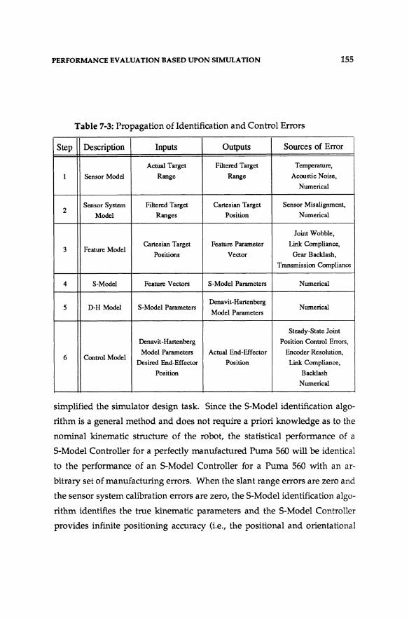
PERFORMANCE EV ALUA TION BASED UPON SIMULA nON 155
Table 7-3: Propagation of Identification and Control Errors
Step Description Inputs Outputs Sources of Error
Actual Target Filtered Target Temperature.
1 Sensor Model Range Range Acoustic Noise.
Numerical
2 Sensor System Filtered Target Cartesian Target Sensor Misalignment.
Model Ranges Position Numerical
Joint Wobble.
Cartesian Target Feature Parameter Link Compliance. 3 Feature Model
Positions Vector Gear Backlash.
Transmission Compliance
4 S-Model Feature Vectors S-Model Parameters Numerical
5 D-H Model S-Model Parameters Denavit-Hartenberg
Numerical Model Parameters
Steady-State Joint
Denavit-Hartenberg Position Control Errors.
6 Control Model Model Parameters Actual End-Effector Encoder Resolution.
Desired End-Effector Position Link Compliance.
Position Backlash
Numerical
simplified the simulator design task. Since the S-Model identification algo
rithm is a general method and does not require a priori knowledge as to the
nominal kinematic structure of the robot, the statistical performance of a
S-Model Controller for a perfectly manufactured Puma 560 will be identical
to the performance of an S-Model Controller for a Puma 560 with an ar
bitrary set of manufacturing errors. When the slant range errors are zero and
the sensor system calibration errors are zero, the S-Model identification algo
rithm identifies the true kinematic parameters and the S-Model Controller
provides infinite positioning accuracy (i.e., the positional and orienta tiona 1

156 PERFORMANCE EVALUATION BASED UPON SIMULATION
deviation between the desired and actual location of the end-effector is zero
for all points within the workspace of the Puma 560).
In order to initiate the simulator, a variety of input parameters must be
specified such as the true locations of the target points with respect to the
links, and the spatial transformation between the sensor coordinate frame
and the robot base coordinate frame. A list of the input parameters and the
values used in our simulation experiments are included in Appendix F.2.
These values coincide with our hardware implementation of the 5-Model
identification algorithm and our prototype system.
We highlight the sequence of computational tasks performed by the
simulator. First, the Puma 560 design model is used to compute the actual
locations of the target points with respect to the sensor coordinate frame.
Then, the actual slant ranges are computed based upon the known positions
of the microphones. Next, zero mean gaussian noise is added to each of the
slant ranges. The standard deviation of this noise depends upon the range.
The linear approximation
o = 9.6432e-SX + 0.003 (7.9)
models the relationship between the noise standard deviation, 0, and the
range, X. In (7.9), 0 and X are measured in centimeters. The corrupted slant
ranges are also quantized to two decimal places to simulate the limited
resolution of the GP-8-30. Using these corrupted slant ranges, the 5-Model
identification algorithm is applied to determine the robot's arm signature.
This procedure is repeated 500 times producing SOD arm signatures. The
Newton-Raphson algorithm is then applied to control the actual Puma 560
robot in performing the grid touching task described in Section 7.2.1 based
upon each of the identified signatures. Finally, the means, variances, and
standard deviations of the thirty four performance indices are computed and
tabulated for later analysis.
PERFORMANCE EVALUATION BASED UPON SIMULATION 157
7.3. Simulator Verification
The goal in verifying the simulator is to demonstrate that is produces
realistic and reliable data. Our simulator id divided into two independent
parts, one which deals with the performance of a D-Model Controller and
one which deals with the performance of an S-Model Controller. The
verification of each these parts can be performed independently.
In verifying the former part we would like to demonstrate that the
statistical performance of a D-Model Controller predicted by the simulator is
consistent with the statistical performance of actual Puma 560 robots which
utilize design model based control. To accomplish this task, we would nor
mally want to vary one or more of the input parameters to both the physical
system and the simulator, monitor the outputs of both the physical system
and the simulator, and then compare the two. Unfortunately in our case,
there are no parameters of the real system which can be varied so as to effect
the performance of the robot. Manufacturing errors are physically em
bedded and fixed within the physical structure of each robot. Furthermore,
we cannot realistically compare the statistical performance of only seven
robots with that of the simulator since a sample size of seven can hardly be
considered statistically meaningful. Although the observed performance of
the seven Puma 560 robots is consistent with the performance distributions
predicted by the simulator additional studies would be required to
rigorously verify the manufacturing error model (7.1).
Verification of the sensor error model and simulated signature iden
tification process is more easily accomplished. Experiments were conducted
in which the calibrated distance, WA,c ' between Microphones A and C (refer
to Appendix E) is intentionally misaligned. The alignment errors ranged
from -1.0 to 1.0 em. While alignment errors of this magnitude are unlikely in

158 PERFORMANCE EVALUATION BASED UPON SIMULATION
practice, their use ensures that the measured variations in the performance of
a robot is statistically significant in comparison to the variability due to other
random errors. In the laboratory, the alignment errors are produced by
modifying the calibration data used by the triangulation algorithms. For
each of eleven different alignment errors we identify the arm signature of
one of the robot's in the laboratory and apply the signatures to control the
position and orientation of the end-effector. The one-dimensional grid
touching task is performed in several times and a cathetometer is used to
measure the performance. The analogous experiments are conducted in
simulation.
The simulated and experimentally measured performance of the Puma
560 is plotted as a function of the error in WA,c in Figure 7-3. In Figure 7-3,
performance is measured in terms of line length error. Line length errors for
three lines are shown: one parallel to the base X axis which is 60.0 cm long,
one parallel to the Y axis which is 40.0 cm long, and one parallel to the Z axis
which is 50.0 cm long. The simulated performance curves represent the
mean performance and the vertical bars (i.e., confidence intervals) delineate
the 3 standard deviation confidence bands [29]. These results confirm that
the simulator produces realistic and reliable data. The experimentally
measured performance curves lie within the confidence intervals of the
simulated performance curves over most of the range in WA,c' It is only for
extreme errors in WA c that the correspondence between the simulator and
the actual performance differ significantly. In practice, such extreme align
ment errors would not occur.

PERFORMANCE EV ALUA TION BASED UPON SIMULATION 159
e-~
g ILi -S r -a
" .s -a
e-~ .. £ -S ~ " -a
" :5
"[ .... .. £ -S r -a
~
0.6 Measured Simulated
-0.4
-0.6
W(A,C) Error (em)
0.8
0.6 Measured Simulated
-0.2
-0.4 '~, * -0.6 '¢"
-0.8 '¢
W(A,C) Error (em)
0.6 ~"
0.4 Measured Simulated
-0.6
W(A,C) Error (em)
Figure 7-3: Simulated and Experimental Performance as a Function of Errors in WA c (a) X Axis Line (b) Y Axis Line (c) Z Axis Line '

160 PERFORMANCE EV ALUA nON BASED UPON SIMULA nON
7.4. Results
Our analysis of the statistical effect of manufacturing errors and iden
tification errors upon end-effector positioning accuracy is divided into five
sections. In Section 7.4.1, we consider the effects of encoder calibration er
rors upon the performance of the D-Model Controller. The effects of machin
ing and assembly errors upon the performance of the D-Model Controller are
discussed in Section 7.4.2. Section 7.4.3 discusses the relationship between
the performance of the S-Model Controller and the sensor system accuracy.
The relationship between the number of measurements and the performance
of the S-Model Controller is described in Section 7.4.4. Section 7.4.5
describes the relationship between the target radii and the performance of
the S-Model Controller.
7.4.1. Encoder Calibration Errors
The procedure for calibrating the joint encoders of a Puma 560 can
often lead to significant encoder calibration errors. These errors result in
fixed biases between the actual and measured positions of the joints. Five
simulations were conducted using model (7.1) to evaluate the effect of ran
dom encoder calibration errors upon robot performance. In these simula
tions, the positional error standard deviation and orientational error stan~
dard deviation were 00=.01 em and 0p=.Ol deg, respectively. The standard
deviation of the encoder calibration error 0e was varied from 0.1 deg to 0.5
deg. The statistical variations in the performance indices of 500 simulated
robots are plotted as a function of 0e in Appendix G.
The standard deviations of all 34 performance indices are seen to in
crease linearly as the standard deviation of the encoder calibration errors
increase. To illustrate, the radial position errors at Vertices 1,4,5, and 8 are

PERFORMANCE EVALUATION BASED UPON SIMULATION 161
l' ~ e CI)
~ ... ,a "'Ci
&!
0.50
0.45
0.40
0.35
0.30
0.25
0.20
0.15
0.10
0.05
0.00 0.10 0.15
at Vertex 1 at Vertex 4 at Vertex 5 atVert&x8
0.20 0.25 0.30 0.35
.+ .El
_x
0.40 0.45 0.50 Encoder sro (deg)
Figure 7-4: Radial Position Error Standard Deviations as a function of (Jt
plotted as a function of (Jt in Figure 7-4. From Figure 7-4, it is also observed
that the rate at which different index standard deviations increase varies.
For instance, the standard deviation of the Vertex 1 radial position error
increases 1.4 times faster than that at Vertex 4. It is believed that the
variability in the rate at which the the performance index standard devia
tions increase as the encoder calibration error standard deviation increases is
partly due to the variability in robot performance over the workspace.
Robots with revolute joints, particularly those with revolute joints in the
positioning system (i.e., the first three joints), tend to amplify joint position
ing errors. Roughly speaking, the amplification factors are the effective radii
between the axes where the errors occur and the end-effector. Thus, as a
robot extends its reach the various amplification factors tend to increase. In
design model control, encoder calibration errors translate into joint position-

162 PERFORMANCE EV ALUA nON BASED UPON SIMULA nON
ing errors. Thus, we would expect robot kinematic performance to decrease
as the desired end-effector position approaches the outer limits of the robot's
workspace. Figure 7-4 and the remaining plots in Appendix G clearly sup
port this hypothesis. The standard deviation of the radial error at Vertices 4
and 8 are .299 cm and .282 cm, respectively, while the standard deviation of
the radial error at Vertices 1 and 5 are .225 cm and .202 cm, respectively -
when a;=O.3deg. From Table 7-1 we see that Vertices 4 and 8 lie near the
maximum reach of the Puma 560 while Vertices 1 and 5 lie relatively close to
the base of the robot.
There is another important feature of the effect of manufacturing errors
upon performance which is not apparent from the plots in Appendix G.
Even though the simulated manufacturing errors have zero mean, the means
of the performance indices are nonzero. In fact for certain performance
indices, the indices' mean values may be larger than their standard devia
tions. Furthermore in some cases, the index means vary linearly with the
encoder calibration error standard deviation. Examples of this are illustrated
in Figure G-2.
The mean value of the Line 11 line length error decreases from 0.0268
cm to 0.0038 cm as ae increases from 0.1 deg to 0.5 deg. Other index mean
values may even change sign. Robot kinematics, especially those of the
Puma 560, are highly nonlinear and coupled. As is often the case for non
linear systems, the expected value of the system output, in this case robot
performance, is both a function of the mean and standard deviation of the
input noise. These results are in direct contradiction to the analytic results
derived by Wu [32]. Our results indicate that in the presense of zero-mean
gaussian random manufacturing errors the expected positioning accuracy of
an arbitrary robot will be nonzero. While a reduction in manufacturing
errors will tend to increase robot positioning accuracy, this approach by itself

PERFORMANCE EVALUATION BASED UPON SIMULATION 163
will not necessarily eliminate the expected positioning errors inherent to
robots which utilize a design model control strategy.
7.4.2. Machining and Assembly Errors
To evaluate the effect of positional and orientational machining and
assembly errors upon robot performance, five more simulations were per
formed. In these simulations, the standard deviations of the positional and
orientational errors, CIp and CIo were varied simultaneously from 0.01 cm and
0.Q1 deg to 0.05 cm and 0.05 deg, respectively, while the encoder calibration
error standard deviation, CIe ' was fixed to 0.1 deg. The standard deviations
of the 34 performance indices are plotted in Appendix G as a function of CIp
and CIo' These sample standard deviations are based upon the performance
of 500 robots.
The variations in the performance index standard deviations in these
simulations are quite different from those in Section 7.4.1. For instance,
consider Figure 7-5 where the radial position error standard deviations at
Vertices 1, 4, 5, and 8 are plotted as a function of CIp and CIo' In contrast to
Figure 7-4, the relationships shown in Figure 7-5 are distinctly nonlinear.
Similar nonlinear relationships are exhibited by the remaining performance
index standard deviations in Figure G-3. Except for the Vertex 1 and Vertex
4 absolute orienta tiona I error standard deviation, the performance index
standard deviations all increase monotonically as CIp and CIo increase. Fur
thermore, the slopes of all 34 curves increase monotonically.
In further contrast to the curves in Figure 7-4, the curves in Figure 7-5
do not all diverge from one another. For example, as CIp and CIo increase the
difference between the variability in the radial positioning error at Vertex 1
and at Vertex 5 decreases from 0.0224 to 0.0138. In some cases the curves
may even intersect as shown in Appendix G.

164
E' ~
e fI) .. ~
LIj -,!! -c &!
0.15
0.14
0.13
PERFORMANCE EVALUA nON BASED UPON SIMULA nON
at Vertex 1 at Vertex 4 at Vertex 5 at Vertex 8
0.12
0.11
,EJ- - •• '
-- - - - - -~.~.~.~~ ... "'~ ~.+., ..
0.10
0.09
0.0&010
Figure 7-5: Radial Position Error Standard Deviation as a Function of C1p and C10 "
The variations in the performance index means as a function of C1p and
C10 are much more predictable than when as a function of C1e" As C1p and C10
increase, all of the performance index means increase monotonically. Plots
of the performance index means as a function of C1p and C10 are presented in
Figure G-4. For Controller D, the presence of positional and orientational
manufacturing errors leads to an average decrease in end-effector position
ing accuracy.
The effect of positional and orientational manufacturing errors on the
variability of end-effector positioning accuracy is more complex than that for
encoder calibration errors as evidenced by the nonlinear relationships in
Figure 7-5. However, the effect of these manufacturing errors upon the

PERFORMANCE EVALUATION BASED UPON SIMULATION 165
expected end-effector positioning accuracy of a robot is much more simple
than for the effect due to encoder calibration errors. Finally, the sensitivity of
the performance index standard deviations to simultaneous variations in (Jp
and (fo is less than the sensitivity of the performance index standard devia
tions to variations in (fe'
7.4.3. Sensor Measurement Errors
Equations (6.12) and (6.13) describe the relationship between feature
estimate accuracy and the sensor system accuracy, (f, as well as the iden
tification parameters, Nj and Rj • Unfortunately, the effect of feature estimate
accuracy upon the performance of an S-Model Controller cannot be derived
analytically. Therefore, the simulator described in Section 7.2.3 was applied
to empirically determine the qualitative relationship between measurement
noise standard deviation, (f, and the expected performance of a Puma 560
robot which uses signature-based control. Six separate simulations were
conducted each using a different values of (f in (7.9), to identify the robot's
arm signature. In each simulation, the value of (f was computed according to
(7.9) and then multiplied by a factor k ranging from 1.0 to 10.0.
The standard deviations of the 34 performance indices as function of k
are plotted in Appendix G. The plot of the Radial Position Error standard
deviation is reproduced below in Figure 7-6. The standard deviations of all
the performance indices increase linearly with the noise measurement factor.
The more inaccurate the sensor system is the more inaccurate the identified
Signatures are and hence the greater the variability in the performance of the
5-Model Controller. The significance of these results is that the sensitivity of
the performance of the S-Model Controller to variations in sensor system
accuracy is consistent with the relationships (6.12) and (6.13) which govern
the feature estimate accuracy. The orientational accuracy of the estimated

166
E' .!:!. e II) .. g LI.j
i " &!
PERFORMANCE EV ALUA TION BASED UPON SIMULATION
0.25
at Vertex 1 .El at Vertex 4
at Vertex 5
- - - -- at Vertex 8
0.10
Figure 7-6: Radial Position Error Standard Deviation as a Function of the Measurement Noise Factor k
planes-of-rotation (6.12) and the positional accuracy of the estimated centers
of-rotation (6.13) are both directly proportional to the measurement noise
standard deviation. Feature estimate accuracy has a direct impact upon the
performance of an S-Model Controller.
Nineteen of the Performance indices are defined such that they can
take on any real value (e.g., the various Line Length Error indices). Using
S-Model control the mean values of these nineteen indices are all zero which
is in strong contrast to the effect which manufacturing errors have upon the
performance of the D-Model Controller. The significance of this is that on
the average we can expect the S-Model identification algorithm to correctly
identify the true kinematic parameters of a robot and thus eliminate end
effector positioning errors. For the remaining 15 perfonnance indices, the
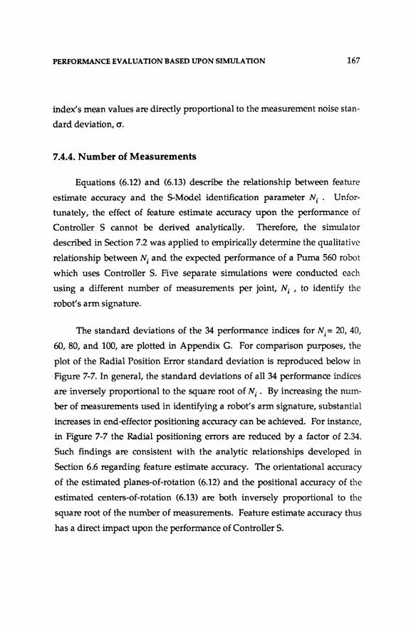
PERFORMANCE EVALUATION BASED UPON SIMULATION 167
index's mean values are directly proportional to the measurement noise stan
dard deviation, cr.
7.4.4. Number of Measurements
Equations (6.12) and (6.13) describe the relationship between feature
estimate accuracy and the S-Model identification parameter Ni . Unfor
tunately, the effect of feature estimate accuracy upon the performance of
Controller S cannot be derived analytically. Therefore, the simulator
described in Section 7.2 was applied to empirically determine the qualitative
relationship between Ni and the expected performance of a Puma 560 robot
which uses Controller S. Five separate simulations were conducted each
using a different number of measurements per joint, Ni ' to identify the
robot's arm signature.
The standard deviations of the 34 performance indices for Ni= 20,40,
60, 80, and 100, are plotted in Appendix G. For comparison purposes, the
plot of the Radial Position Error standard deviation is reproduced below in
Figure 7-7. In general, the standard deviations of all 34 performance indices
are inversely proportional to the square root of Ni . By increasing the num
ber of measurements used in identifying a robot's arm signature, substantial
increases in end-effector positioning accuracy can be achieved. For instance,
in Figure 7-7 the Radial positioning errors are reduced by a factor of 2.34.
Such findings are consistent with the analytic relationships developed in
Section 6.6 regarding feature estimate accuracy. The orientational accuracy
of the estimated planes-of-rotation (6.12) and the positional accuracy of the
estimated centers-of-rotation (6.13) are both inversely proportional to the
square root of the number of measurements. Feature estimate accuracy thus
has a direct impact upon the performance of Controller S.

168
e-~
e (/) .. 2 Lij -.!! "b
~
PERFORMANCE EVALUATION BASED UPON SIMULATION
0.055
0.050 , at Vertex 1 , at Vertex 4 , _ .. - _ ... , at Vertex 5 0.045 , - - - ---, at Vertex 8 , - - ---,
0.040 , , 's
0.035 "-
0.030
0.025
0.020 -+ ---------.. -+- . ---. ------. + ~ ~--~~- - - - - ~ 0.015 ----+
0.010 +--~--.,.--.....,--.....,r----r---'T"""---r---., 20 30 40 50 60 70 80 90 100
NumptslClrcle
Figure 7-7: Radial Position Error Standard Deviation as a Function of the Number of Points per Circle, Ni
Consider again the nineteen performance indices which are defined
such that they can take on any real value. Using signature-based control the
mean values of these nineteen indices are all zero (Le., negligible in com
parison with the corresponding standard deviations) which is in strong con
trast to the effect which manufacturing errors have upon the performance of
D-Model Control. On the average we can expect the S-Model identification
algorithm to correctly identify the true kinematic parameters of a robot and
thus eliminate end-effector positioning errors. For the remaining 15 perfor
mance indices, the index's mean values are inversely proportional to the
square root of Ni as illustrated in Appendix G.

PERFORMANCE EV ALUA TION BASED UPON SIMULATION 169
7.4.5. Effect of Target Radius
In this section, we apply the simulator used in the previous section to
analyze the relationship between end-effector positioning accuracy and the
target radii. Naturally, the values of certain target radii will have greater
impact upon the overall performance of the robot than will others. Since it
would be impractical to simulate all the possible combinations of the values
of the six target radii and interpret the results, we have limited our analysis
to the situation in which all the target radii are equal. Thus in each simula
tion, Rl = R2= ... = R6= R/IOm. Five simulations were performed in which
the value of Rnom is varied between 30.0 cm and 50.0 em. The standard
deviations of the 34 performance indices as a function of R/IOm are plotted in
Appendix G. The plot of the Radial Position Error standard deviations is
reproduced in Figure 7-8.
While the parameter Ni has an effect upon both the accuracy of the
identified planes-of-rotation and centers-of-rotation, the parameter R/IOm only
effects the accuracy of the planes-of-rotation. Taken independently, Ni and
Rnom are both inversely proportional to the accuracy of the identified planes
of-rotation. From the findings in the previous section we might thus expect
that increasing Rnom would have less of an overall effect upon the perfor
mance index standard deviations than does Ni • However, from Figure 7-8
and the plots in Appendix G this is not the case. The curves in Figure 7-8 are
approximated more closely by an inverse square relationship rather than by
an inverse relationship. The cumulative accuracy of an identified arm Sig
nature appears to be more sensitive to orientational errors than poSitional
errors. This could be explained by the fact that orientational errors, espe
cially those involved in the description of a manipulators positional subsys
tem, not only propagate into orientational errors at the end-effector but they
are also transformed and amplified into positional errors at the end-effector.

170
i' .a e II)
~ t:
1£.1 -~ ~
0.060
0.04
0.03
0.025
0.020
0.015
, , , , , , , , ,
PERFORMANCE EVALUATION BASED UPON SIMULATION
at Vertex 1
- -- - --- - _. at Vertex 4
- - - - - -- at Vertex 5
------ at Vertex 8 , " " '0..
" "
.+- .
Figure 7-8: Radial Position Error Standard Deviation as a Function of Target Radius
The amount of amplification being proportional to the lengths of the links
and the configuration of the robot.
The variations in Rnom have no effect upon the mean values of the
standard deviations of the performance indices which are defined over all
the real numbers. As in the previous section, the mean values for these 19
performance indices are zero. For the remaining 15 performance indices, the
indices' mean values are, in general, inversely proportional to R!'m as il
lustrated in Appendix G.
These findings suggest that the best strategy for increasing signature
accuracy is to first increase the target radii followed by increases in the
number of measurements. The cost of increasing the number of measure-

PERFORMANCE EVALUATION BASED UPON SIMULATION 171
ments is the increased time required to obtain all the target measurements.
This cost is incurred during the identification of each individual signature.
In contrast, the cost associated with increasing Rnom is simply the reconstruc
tion of a set of target mounting fixtures. This cost has only to be incurred
once since a single set of fixtures can be applied to all robots of the same
model.
7.5. Conclusions
In this chapter, we have formulated a methodology by which to
evaluate and compare the statistical performance of a conventional design
model-based kinematic controller and a signature-based kinematic con
troller. The design model controller incorporates the robot kinematic
parameters obtained from the mechanical design specifications. In contrast,
the signature-based controller incorporates the robot kinematic parameters
estimated by the S-Model identification algorithm. Furthermore, we have
applied this methodology to evaluate and compare the statistical perfor
mance of these two controllers when applied to control the joint positions of
a Puma 560 robot. This work complements our experimental evaluation of
the performance of seven Puma 560 robots which was described in Chapter
6.
Our methodology utilizes Monte-Carlo simulation techniques for the
generation of end-effector positioning and orienting error distributions. The
evaluation of the performance of the D-Model Controller, requires the for
mulation of a robot kinematic model which explicitly incorporates the
manufacturing errors as parameters. A kinematic model of a Puma 560 robot
with manufacturing errors was developed and serves to illustrate how such
a model could be developed for other robots. The performance of the S
Model Controller depends upon the types of the errors introduced into the

172 PERFORMANCE EVALUATION BASED UPON SIMULATION
arm signature identification process and not upon the presense of robot
manufacturing errors. Having developed a model of our ultrasonic sensor
system, we simulated the arm signature identification process using a Puma
560 robot and applied the identified signatures to control the robot in per
forming a series of standardized tasks. The positioning and orienting ac
curacy of the end-effector is used to evaluate of how well S-Model Controller
performed. This approach can be applied to analyze the statistical perfor
mance of the 5-Model Controller for any robot with any type of sensor sys
tem by interchanging simulator modules. In Section 7.3, we devised experi
ments to verify that our simulator produced realistic and reliable results.
In Sections 7.4.1 and 7.4.2, we applied our Monte-Carlo simulator to
investigate the relationship between encoder calibration errors and robot
performance, and the relationship between machining and assembly errors
and robot performance, respectively. From this investigation we have dis
covered that
• The performance indices standard deviations increase linearly with the standard deviation of the encoder calibration errors.
• The performance indices standard deviations increase nonlinearly and monotonically with simultaneous changes in the standard deviations of the positional and orientational manufacturing errors.
• The performance of a D-Model Controller is more sensitive to encoder calibration errors than to the positional and orientational manufacturing errors.
• The expected performance of a D-Model Controller is a function of both the means and standard deviations of the manufacturing errors.
In practice then, the average performance of a robot using design model
based control will be less than perfect. This finding clearly supports our

PERFORMANCE EVALUATION BASED UPON SIMULATION 173
claim that arm signature identification techniques are needed to improve
end-effector positioning and orienting accuracy.
In Sections 7.4.3 - 7.4.5, we have also applied our Monte-Carlo
simulator to understand the relationships which govern the performance of
an S-Model Controller. Specifically, we were interested in the relationships
between the sensor system accuracy, the identifier parameters N j and R j , and
the end-effector positioning accuracy. We have found that,
• The performance indices' standard deviations are directly proportional to the sensor measurement error standard deviation <J and that this relationship is consistent with the analytic relationships between <J and the measures of feature estimate accuracy derived in Section 6.6.
• The performance indices' standard deviations are inversely related to the square root of the number of measurements, N j and that this relationship is consistent with the analytic relationships between Nj and the measures of feature estimate accuracy derived in Section 6.6.
• The performance indices standard deviations are inversely related to the square of the target radii.
• The performance of an S-Model Controller is more sensitive to orientational identification errors than to positional identification errors.
• The expected performance of an 5-Model Controller depends only upon the expected value of the measurement errors.
The identifier parameters, N j and R j , provide a simple mechanism for in
creasing the accuracy of the identified arm signatures and hence the perfor
mance of an 5-Model Controller by a predetermined amount. Conversely,
then can be used to reduce the need for extremely accurate sensor systems to
measure the targets positions. Finally, the 5-Model identification algorithm
and control approach will, on the average, provide perfect end-effector

174 PERFORMANCE EV ALUA TION BASED UPON SIMULATION
positioning and orienting accuracy in the presense of zero-mean target
measurement errors. The elimination of biases in the expected performance
of a robot is a important advantage of the our approach.

ChapterS
Summary and Conclusions
8.1. Introduction
In this chapter, we summarize (in Section 8.2) our contributions and
identify (in Section 8.3) areas for future research.
8.2. Summary and Contributions
In this section, we review and enumerate the contributions of the dis
sertation. Our research and contributions lie in three areas: robot kinematic
modeling, robot kinematic parameter identification, and robot kinematic control.
We proceed through the development of the dissertation.
In Chapter 2, we reviewed robot kinematic modeling, identification,
and control techniques, and established a framework in which to present our
research contributions. The fundamental problem in the development of
robot kinematic models is the use of geometric and trigonometric principles
to systematically specify the relative positions and orientations of robot
jOints. The goal of a kinematic identification algorithm is to identify the
parameters of a kinematic model which describe the actual position and
orientation of the end-effector in terms of the measured joint positions, and
which incorporates the geometrical variations in the structure caused by
manufacturing errors . The kinematic control problem focuses upon the
computation of the joint positions required to locate the end-effector at a
desired Cartesian position and orientation.

176 SUMMARY AND CONCLUSIONS
In Chapter 3, we introduced the formulation and properties of a new
model for describing the kinematic structure of any robotic manipulator with
rigid links. This kinematic model, which we call the S-Model, is designed
to facilitate kinematic parameter identification. Like the Denavit-Hartenberg
model, which has had widespread application to robot control, the S-Model
is conceptually based upon the assignment of Cartesian coordinate frames
fixed relative to each of the liI1ks. The S-Model possesses three important
features which make it directly applicable to kinematic identification. First,
there is a considerable amount of flexibility in assigning the locations of the
link coordinate frames. Second, the locations of the link coordinate frames
are independent of the locations of the other link coordinate frames. And
third, the Denavit-Hartenberg parameters can be easily extracted from the
S-Model parameters.
In Chapter 4, we formulated the S-Model identification algorithm
which can be applied to identify the kinematic parameters of any robot with
rigid links. The objective of S-Model identification is to estimate the S-Model
kinematic parameters from a set of 2nr+np kinematic/mechanical features
inherent to the manipulator, where nr is the number of revolute joints and np
is the number of prismatic joints. The kinematic features of a revolute joint
are a plane-of-rotation and a center-of-rotation, and the kinematic feature of
prismatic joint is a line-of-translation. The S-Model identification algorithm
consists of four steps. The first step involves the explicit identification of the
robot's kinematic features from measurements of the Cartesian position of
targets placed on the robot's links. In the second step, the identified features
are used to establish the positions and orientations of the S-Modellink coor
dinate frames with respect to the sensor coordinate frame. In the third step,
the elements of the S-Modellink transformation matrices are evaluated and
used to solve for the 6'n S-Model parameters. Finally, in the fourth step, the
robot's Denavit-Hartenberg parameters are determined. The advantage of

SUMMARY AND CONCLUSIONS 177
the 5-Model identification algorithm is that it decouples the robot kinematic
identification problem into a set of simpler identification problems which
can be solved using standard linear regression techniques.
In Chapter 5, we presented two algorithms for inverting general arm
signature models and compared both their numerical performance and com
putation complexity. The inverse kinematic problem requires the solution of
a set of n coupled nonlinear equations. The first algorithm is based upon
Newton's method and the second algorithm is the Jacobi iterative algorithm
applied specifically to the inversion of signature models.
In Chapter 6, we developed a complete prototype arm signature iden
tification system and applied it improve the performance of seven Puma 560
robots. This system incorporates an ultrasonic range sensor (described in
Section 6.3) to measure the three-dimensional Cartesian positions of the tar
get sparkers placed on the robors links. The relative Cartesian positioning
accuracy of the sensor system is approximately ± 0.02 em. The general
characteristics of the sensor design and the overall system design, which
exploits averaging over many sensor readings, offer numerous advantages
for arm signature identification. In this chapter, we also applied the
prototype system to improve the kinematic performance of seven Puma 560
robots. Three methods were devised to evaluate manipulator kinematic per
formance during which the Puma is programmed. to position its end-effector
at the vertices of a one-, two-, or three-dimensional grid. At each of the grid
vertices, the actual relative poSition of the end-effector is measured. In the
three-dimensional case, the actual relative orientation of the end-effector is
also measured. For these robots, relative end-effector positioning and orient
ing accuracy was improved on the average by a factor of 5-10.
In Chapter 7, we considered the statistical performance of robot posi-
178 SUMMARY AND CONCLUSIONS
tion control methods, and discussed the origin of robot positioning errors. In
conventional design-model robot control, manufacturing errors contribute
most to robot positioning errors. With arm signature-based robot control,
robot performance is limited by sensor errors which contribute to the in
accuracy of the identified arm signature model. Monte-Carlo simulation
techniques have been applied to study the relationship between the perfor
mance of design model control and manufacturing errors and the relation
ship between the performance of signature-based control and target
measurement errors.
We believe that the contributions of this dissertation are:
• The design (in Chapter 3) of a new robot kinematic model for describing the relationship between the Cartesian position and orientation of the end-effector and the robot base coordinate frame as a function of the joint positions and a set of fixed kinematic parameters. In contrast to other models, our model called the S-Model is directly applicable to the kinematic identification problem. The analytic relationship between S-Model and the Denavit-Hartenberg Model is also derived.
• The identification (in Chapter 4) of the three mechanical/kinematic features of robotic manipulators. The plane-of-rotation and center-of-rotation features describe the behavior of revolute joints and the line-of-translation feature describes the behavior of prismatic joints. These features inherently describe the kinematic structure of a robot and provide a foundation for the design of the S-Model kinematic parameter identification algorithm.
• The development (in Chapter 4) of a general and practical technique for identifying the kinematic parameters of any robotic manipulator with rigid links. The technique, called the S-Model identification algorithm, uses measurements of the Cartesian position of targets placed on the robot's links and in the absence of measurement noise will identify the true kinematic parameters of a robot including the geometrical variations in the structure caused by robot manufacturing errors.

SUMMARY AND CONCLUSIONS
• The fonnulation of the Newton-Raphson and Jacobi Iterative algorithm (in Chapter 5) for solving the inverse kinematics problem for robots with non-simple kinematic structures. The convergence properties of both algorithms have been studies and compared based upon simulation results. The computational burden of both algorithms is also assessed. The Newton-Raphson algorithm is applied (in Chapter 6) to control the end-effector of several Puma 560 robots using identified ann signature parameters .
• The implementation of a complete prototype ann signature identification system. This prototype system has been applied (in Chapter 6) to improve robot end-effector positioning accuracy. The contributions derived from the implementation are:
• The design (in Chapter 6) of an ultrasonic range sensing system to measure the three-dimensional positions of targets attached to the links of the robot. The targets are implemented by an ultrasonic source (sparker) and an array of four ultrasonic range detectors are used to measure the time-of-flight of the emitted ultrasonic wave.
• The identification of the arm signatures of seven Puma 560 robots.
• The introduction of three methods for evaluating robot kinematic performance. These methods, referred to as the one-, two-, and three-dimensional grid touching tasks, provide a practical means for evaluating robot kinematic performance using relatively inexpensive equipment.
• The comparative evaluation of the actual perfonnance of the Puma 560 robots using design model based control and signature-based control. As anticipated the identified arm signatures significantly improved the performance of all seven robots in comparison to their perfonnance with design model based control.
• The demonstration of the applicability and practicality of the S-Model identification algorithm towards improving robot end-effector positioning and orienting accuracy.
• The fonnulation of general methodology (in Chapter 7) for
179

180 SUMMARY AND CONCLUSIONS
evaluating and comparing the statistical performance of robots using design model based control and signature-based control. The methodology is based upon the use of Monte-Carlo simulation techniques to generate end-effector positioning and orienting errors arising from the presence of either robot manufacturing errors or measurement errors in the kinematic parameter identification process. This formulation included:
• The development (in Chapter 7) of a technique for modeling the kinematics of robots with manufacturing errors. We apply this technique to a Puma 560 and use the resulting model to analyze the effects (in Sections 7.4.1 and 7.4.2) of random manufacturing errors upon end-effector poSition accuracy .
• The evaluation and comparison (in Chapter 7) of the statistical performance of a Puma 560 robot using design model based control and signature-based control. The evaluation leads to design guidelines for specifying the signature identification parameters (Le., the target radii and the number of measurements) and the accuracy of the sensor system used to obtain the target measurements.
8.3. Suggestions for Future Research
We suggest the following research directions to extend the contribu
tions of this dissertation:
• The development of alternative sensor systems for measuring the three-dimensional positions of the targets attached to the robot's links. The performance of the S-Model identification algorithm is limited by the accuracy of the sensor system. The ultrasonic sensor system used in our prototype system is believed to have an accuracy of approximately ± 0.02 em. This estimate of the accuracy was obtained indirectly, however, since the physicallocations of the reference surfaces of the microphones are impossible to specify. We suspect that there are in fact small biases in the individual range measurements but have been unable to derive a method for identifying them. Methods for measuring and/or
SUMMARY AND CONCLUSIONS
identifying the biases in such systems are needed to further improve the accuracy of identified arm signatures using ultrasonic range measurements. The presence of such biases eventually lead to bias errors in the estimated target positions and hence limit the accuracy of the identified signatures.
• The development of techniques for modeling and identifying the kinematics of robots with compliance.
• The development of customized and systematically-organized algorithms to reduce the computational requirements for the online implementation of the Newton-Raphson and Jacobi Iterative Iterative algorithms.
• The development of special purpose hardware for implementing kinematic control algorithms to reduce the overall controller sampling rate. As mentioned in Chapter 5 a significant percentage of the computations required by the Jacobi Iterative algorithm can be performed in parallel. Computer architectures specifically designed to exploit this structure and/or the structure of other kinematic inversion algorithms would be of great interest to the robotics community.
181
We believe that progress in these directions will extend the contributions of
this dissertation thus leading to further improvements in robot kinematic
performance and will hopefully expand the range of robotic applications.

Appendix A
Primitive Transformations
The six primitive homogeneous transformations matrices are
1 0 0 x 0 1 ° 0
Trans(x, 0, 0) 0 ° 1 0 0 0 0 1
1 0 0 0 0 1 0 Y
Trans(O, y, 0) 0 ° 1 0 0 0 0
1 0 0 ° 0 1 0 0 Trans(O, 0, z) 0 0 1 z
0 ° 0 1
1 0 ° ° 0 cose - sine ° Rot(x, e) 0 sine cos9 0 0 0 0 1

184 PRIMITIVE TRANSFORMATIONS
cose 0 sine 0 0 1 0 0
Rot(y, e) = - sine 0 cose 0
0 0 0 1
cose - sine 0 0 sine cose 0 0
Rot(z, e) 0 0 1 0 0 0 0 1

AppendixB
Ideal Kinematics of the Puma 560
The following sections list the forward and inverse kinematic relations
for Puma 560 robot assuming negligible manufacturing errors (i.e., the ideal
kinematics). A derivation of the inverse kinematics can be found in [19]10.
B.1. Forward Kinematics
The forward kinematics of the Puma 560 robot are defined by the
matrix
T6
where
n" =
ny =
nz
OX =
llx Ox ax Px
lly Oy a y Py
llz Oz ~ pz
0 0 0 1
C1 [C23 (C4CSC6 - S4S6) - SZ3SSC6] -
S1 [S4CSC6 + C4S6]
S1 [C23 (C4CSC6 - S4S6) - SZ3SSC6] + C1 [S4CSC6 + C4S6]
-S23(C4CSC6-S4S6) - C23SSC6
C1 [-C23 (C4CSS6 + S4C6) + S23SSS6]
(B.1)
(B.2)
(BJ)
(BA)
l(}yne derivation in [19] contains two errors which have been oorrected in the above equations.

186 IDEAL KINEMATICS OF THE PUMA 560
SI [-S4CSS6 + C4C6 ] (B.5)
0y SI [-C23 (C4CSS6 + S4C6) + S23SSS6] + C1 [-S4CSS6 + C4C6 ] (B.6)
OZ -S23 (C4CSS6 + S4C6) + C23SSS6 (B.7)
ax CI(C23C4SS+S23CS) - SIS4SS (B.8)
ay SI (C23C4SS + S23CS) + C1S4SS (B.9)
az = -S23C4SS + C23CS (B.IO)
Px = C1 (d4S23 + a3C23 + a2C2) - d3S 1 (B.ll)
Py SI (d4S23 + a3C23 + a2C2 ) + d3C 1 (B.l2)
Pz = -( -d4C23 + ~S23 + a2S2 ) (B.l3)
Si' Ci , Sij' and Cij refer to sin9i , cos9i , sin (9i+9j ) ,and cos (9i+9), respec
tively.
B.2. Inverse Kinematics
The inverse kinematics of the Puma 560, in tenns of the known ele
ments of T6 in (B.1), are
d tan -I 3
(r12 - dl)l!2 (B.l4)
93 (B.l5)
if 9s > 0
(B.l8)

IDEAL KINEMATICS OF THE PUMA S60 187
9S _lC4 [C23 (axCl + aySl) - az S23]
(B.19) = tan + S23 (axCl + aySl ) + azC23
S4[-axS1 + ayC1]
S23(ax C1 + ayS 1) + azC23
96 _l-CS {C4 [C23 (ox C1 +OySl )-ozS231+
= tan -S4 [C23 (oxCl +OySl )-ozS23]
S4[-oxS 1 + 0yCl ]}
+ 0 +
+ SS{S23(Ox C 1+0y S 1)+OzC23 } (B.20)
+ C4 [-ox S 1+0yC1]
where
'I 2 2 1/2 (px + Py) , (B.21)
72 = 2 2 ~ 2 2 (PxCl +PySl) + Pz - 4 - ~ - a2 (B.22)
and
2 2 2;; 73 = 4a2a3 + 4a2 4 (Constant) (B.23)
When 9s=0, the manipulator becomes degenerate. Both the Joint 4 and JOint
6 axes are then aligned. In this case, either 94 or 96 can be chosen arbitrarily.

AppendixC
Inverse Kinematics
C.l. Newton-Raphson Computations
Step 1:
Step 2:
Step 3:
Step 4:
StepS:
Step 6:
Step 7:
Step 8:
Evaluate the elements of the manipulator Jacobian, J, using the method described in [18]. In doing so the forward signature model will also be evaluated (i.e., T6 in (5.1)).
Compute the positional and orientational differential matrix, o!:l, with respect to the manipulator's base coor-dinates. The matrix 0ll.k = T~ - T6.
Invert the matrix T6.
Express differential matrix, 0ll.k, in terms of end-effector coordinates. In other words, compute the elements of the matrix 61l.k = [T6r1 0f:lc.
Express differential matrix, 61l.k, in vector form as denoted by '3k [18].
Solve the system of linear equations '3k = J dq where dq:: qk_qk-1. Update solution vector according to q = q + dq
Check if the elements of the vector dqare less than the resolution of the corresponding joint encoders. If all are then terminate, else return to Step 1.

190 INVERSE KINEMATICS
C.2. Jacobi Iterative Computations
Step 1:
Step 2:
Step 3:
Step 4:
Step 5:
Step 6:
Compute the sines and cosines of the six joint positions.
Compute the forward signature model (Le., the elements of the matrix Fs (q~ in (5.8».
Compute the forward design model (Le., the elements of the matrix Fd(q~ in (5.8».
Invert the forward signature model matrix Fs(ii;).
Multiply the matrices Fd(qj), [Fs(q)rl, and T~. Evaluate the inverse kinematics of the design model (refer to Appendix B) using the matrix evaluated in Step 5 as the input.

AppendixD
Identified Arm Signtaures
Table 0-1: Identified Arm Signature Parameters
Name Link Variable 9olls., (deg) d (cm)
I 91 110.308 -20.678
2 92 79.977 11,210.213
3 93 -79.483 -11,194.976 Robot 3
4 94 -0.296 43.278
5 9s -0.497 -0.018
6 96 -89.081 10.300
I 91 109.570 -20.823
2 92 14.786 1,636.110
Robot 4 3 93 -14.883 -1,621.207
4 94 -0.101 43.388
5 9s 0.106 -0.070
6 96 -89.021 10.275
I 91 110.849 -20.428
2 92 63.467 2,783.580
3 93 -63.276 -2,768.574 Robot 5
4 94 0.328 43.299
5 9s -0.126 -0.054
6 96 -89.517 10.273
a (cm) a. (deg)
-0.005 -90.066
7.6071 -0.217
-2.039 90.519
-0.001 -90.007
0.002 89.990
0.000 0.000
-0.037 -89.992
41.707 -0.394
-2.059 90.002
-0.019 -90.036
-0.011 90.023
0.000 0.000
-0.023 -90.013
19.084 -0.803
-2.028 90.134
-0.009 -89.991
0.007 89.969
0.000 0.000
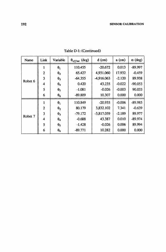
192 SENSOR CAUlJRATlON
Table 0-1: (Continued)
Name Link. Variable 9o//sel (deg) d(cm) a (cm) ex (deg)
1 91 110.455 -20.672 0.013 -89.997
2 92 65.427 4,931.060 17.932 -0.459
Robot 6 3 93 -64.355 -4.916.063 -2.120 89.938
4 94 0.420 43.235 -0.022 -90.053
5 95 -1.081 -0.026 -0.003 90.033
6 96 -89.809 10.307 0.000 0.000
1 91 110.849 -20.935 -0.006 -89.985
2 92 80.179 3,832.102 7.341 -0.639
Robot 7 3 93 -79.172 -3,817.059 -2.189 89.977
4 94 -0.688 43.387 0.010 -89.974
5 95 -1.428 -0.026 0.006 89.994
6 96 -89.771 10.282 0.000 0.000

AppendixE
Sensor Calibration
E.l. Calibration Rods
Two calibration rods are depicted in Figure 6-4. Conceptually, a
calibration rod is an apparatus for securing two sparkers at a known and
fixed distance apart. The nominal distance between these sparkers is 100 cm.
The upper calibration rod contains sparkers 1 and 2, and the lower calibra
tion rod contains sparkers 3 and 4. The upper calibration rod is positioned
such that the tips of sparkers 1 and 2 and the acoustic zero point of
Microphone B are collinear and level. Similarly, the lower calibration rod is
positioned such that the tips of sparkers 3 and 4 and the acoustic zero point
of Microphone D are collinear and level.
These calibration rods provide a means for accurately determining the
speed of sound at a particular instance in time. Assuming that the speed of
sound is constant along the line between Sparker 2 and Microphone Band
along the line between Sparker 4 and Microphone D, the calibration rods
provide a mechanism to accurately estimate the speed of sound at
Microphone Band D. Using the upper calibration rod, the ratio of the speed
of sound at Microphone B to the speed of sound internal to the GP-8-3D, S',
is
(E.1)

194 SENSOR CALIBRATION
= Calibrated distance between sparkers 1 and 2 Measured distance between sparkers 1 and 2
where sl and Sz are the measured slant ranges between Sparker 1 and
Microphone B and Sparker 2 and Microphone B, respectively. The ratios fB
and fD are applied in Section E.2 to compensate the three primary slant range
measurements between the target sparker and Microph<mes A, B, and C.
E.2. Slant Range Compensation
The method we have developed for correcting the slant ranges ob
tained from the GP-8-3D (Le., the raw slant ranges) compensates for both
overall variations in the speed of sound and spatial variations in the speed of
sound. Applying this method, we have achieved relative Cartesian position
ing accuracies on the order of the resolution of the GP-8-3D. The resulting
slant range compensation algorithms are based upon a simplified model of
the operating environment. According to this model,
• The effect of air currents upon the speed of sound is negligible (B-1).
• All variables upon which the speed of sound depends, such as temperature and humidity, vary slowly relative to the time required to gather an individual target measurement (e.g., time constants on the order of minutes) (B-2).
• The temperature of the air within the active region of the sensor varies linearly with vertical height and is constant in the two horizontal directions (B-3).
• The temperature differential between the air at the top and bottom of the sensor's active region is less than 2 OF (B-4).
• The average temperature of the air within the active volume of the sensor is between 65 OF and 75 OF (B-5).
Assumptions (B-1) - (B-5) are consistent with environmental characteristics of
SENSOR CALIBRATION 195
our laboratory at the Robotics Institute of Carnegie-Mellon University. Our
laboratory, originally designed as a computer machine room, is ap
proximately 30 ft x 30 ft with a 12 ft ceiling. Only a small portion of the
laboratory is actually utilized. The room contains a raised floor under which
cooled air from adjacent machine rooms is free to circulate. Due to the lack
of heating or air conditioning vents, the temperature within the room is
governed by the conduction or radiation of heat through the walls to the
adjacent machine rooms. This feature insures that the temperature and
humidity within the room remains relatively constant. Use of the ultrasonic
sensor system for accurate measurements requires attention to these issues.
In practice, robot manufacturers who want to identify the kinematic
parameters of their manipulators as an integral part of the manufacturing
process may enclose the sensor system in a moderately-controlled environ
mental chamber such as that used for testing and qualification.
The relationship between temperature and the speed of sound is ap
proximately linear for small variations in temperature (Le., less than 5 OF).
Thus, according to our model of the environment, the speed at which sound
travels along a straight line between the target sparker and a microphone
(i.e., the line of sight) varies linearly with distance traveled. Thus,
dx - = Jlx + ~2 ' dt
(E.2)
where x=x(t) is the distance traveled by the ultrasonic wave front in time t
(i.e., x(O) =0 at the target), Jl is the rate of change of the speed of sound along
the line of sight, and ~2 is the speed of sound at the microphone. Integrating
(E.2) from time t = 0 to t = t, the actual time of flight, the distance between the
target and microphone

196 SENSOR CALIBRATION
• P2 • x(t) = -[ exp{J1t) - 1] .
Il (E.3)
By definition,
P2-P1 Il = -.-
x(t) (E.4)
where PI is the speed of sound at the target sparker. If the line of sight is
level, then VI = V 2 and the actual slant range x(t) = pl·
Estimates for PI and P2 must be obtained in order to solve (E.3). Using
the upper and lower calibration rods depicted in Figure 6-4, we measure the
speed of sound at two distinct heights (i.e., fB and fD)' Then, based upon the
known relative heights of the microphones and the calibration rods, we
linearly interpolate to estimate the speed of sound at Microphones A, B, and
C. An additional step is required to estimate PI since the height of the target
is initially unknown. The objective of this step is to determine an initial
estimate for the Cartesian coordinates of the target from which an estimate
for its height can be computed. We define the average speed-of-sound ratio
over the active region of the sensor array to be
(E.5)
By multiplying the three raw slant ranges, 81,82' and 83, by (E.5), we compen
sate for overall variations in the speed of sound relative to the nominal value
internal to the GP-8-3D. The compensated slant ranges are used in (6.1) -
(6.6) to compute the initial estimate of the targets Cartesian coordinates. We
then compute the height of the target and linearly interpolate to estimate PI in (E.4).
We apply Jacobi's Iterative algorithm to solve (E.3) for each of the three

SENSOR CALIBRA nON 197
primary slant ranges. The resulting final estimates for the slant ranges are
used in (6.1) - (6.6) to compute the final estimate of the target's Cartesian
coordinates. Our method of compensating the GP-8-3D's slant range
measurements requires that all five sparkers must be sparked at least once to
determine the target's location. Subsequent to the sparking of the sparkers,
the GP-8-3D will transmit twenty slant range measurements to the host com
puter. Only seven of the measurements are used in our algorithms. The
remaining measurements are discarded. In practice, 10-20 sets of slant range
measurements are obtained and statistically averaged to reduce the effects of
random measurement noise inherent in the GP-8-3D.

AppendixF
Simulator Components
F.t. Robot Manufacturing Error Model
To understand the derivation of the model (7.1), consider the task of
manufacturing the actual physical base link of a Puma 560, shown in Figure
F-1.Conceptually, the base link is a cylinder. To manufacture the link, one
end of the cylinder must be machined to a flat surface, the normal of which
should be coincident with the axis of the cylinder. Similarly, the other end
should be machined flat such that the two end surfaces are a desired distance
apart. Then, a bearing race must be mounted within the top of the cylinder
such that the centroid of the bearing is coincident with the end surface and
the axis of the bearing is coincident with the axis of the cylinder. Later on
the base link and Link 1 will be joined. The lower end of Link 1 will contain
the mating portion of the bearing race which is also characterized by an axis
and a centroid. Ideally, during the process the axes and centroids of the two
mating pairs will be perfectly aligned. Similar manufacturing processes can
be envisioned for the remaining links.
Imagine two coordinate frames fixed to the components of the link. Let
the Z axis of the first coordinate frame be coincident with the axis of the
cylinder and let its origin be coincident with the center of the bottom surface
of the cylinder. Let the Z axis of the second coordinate frame be coincident
with the axis of the bearing and let its origin be coincident with the centroid
of the bearing. Kinematically then, a perfectly manufactured base link is

200 SIMULATOR COMPONENTS
(a) (b)
Figure F-l: Base Link of a Puma 560. (a) Actual (b) Conceptual
described by the transformation matrix Trans (0.0, 0.0, 67.4cm). However,
when manufacturing errors are present these two coordinate frames will not
be perfectly aligned. For instance, the bottom surface of the link may not be
precisely perpendicular to the axis of the cylinder. In this case, we can
describe the kinematic structure of the link by the new transformation matrix
Rot (x, £4) Rot (y, £s)Trans(O.O, 0.0, 67.4cm) , (F. 1)
where £1 and Ez represent small random deviations in the orientation of the
machined bottom surface. The machining of the top of the cylinder and the
mounting of the bearing race may lead to similar orientational errors at the
other end of the link. Taking these errors into account (F.l) becomes

SIMULATOR COMPONENTS
Rot (x, £,J Rot (y, £5) Trans (0.0, 0.0, 67.4cm) Rot (x, £~
Rot(y, £.r) •
201
(F.2)
By modifying (F.2) further, to account for possible errors in the length of the
cylinder, errors in locating the center of the base, and errors in calibrating the
joint encoder we arrive at the model (7.2) to describe the actual kinematic
structure of the base link. This same method01ogy has been applied to devel
op the models (7.3) - (7.8) of Links 1 through 6.
F.2. Simulator Input Parameters
This section defines input parameters must be specified in order to
simulate the performance of Controller S. The values for these parameters
which coincide with our prototype arm signature identification system are
also included. Linear parameters are measured in centimeters and angular
parameters are measured in degrees.
The spatial transformation between the sensor coordinate frame and
the robot base coordinate frame is
9Tb = Trans(106.16,56.98,87.82)Rot(z,45.0)
Rot (x,-90.0)Rot (z, 155.0)
Trans(0.O,-20.30,-67.183) . (F.3)
The spatial transformation between the robot base coordinate frame
and the Denavit-Hartenberg Link 0 coordinate frame is
bTO = Trans(0.O,O.O,67.183) (F.4)
Six targets are attached to the robot's links during the identification

202 SIMULATOR COMPONENTS
procedure. By definition, Target i is fixed to Link i. The position of Target i
with respect to the base coordinate frame is specified by the position vector
component of the transformation matrix
(F.5)
where the matrices Aj are the Denavit-Hartenberg link transformation
matrices in (2.9), 0i is the angular position of Joint i , and Ri is the Target i
nominal radius. Values for the nominal target radii are listed in Table 6-l.
The offset transformation matrices
Ojfseti = Trans (0.0, 0.0, zi) . Rot (x, rXi)
for i= 1,2, ... ,6 (F.6)
are defined by the parameters Zj and rXi' The values for these parameters are
listed in Table F-l.
Table F-l: Offset Transformation Matrix Parameters
Parameter Values Transfonnation Zi rXi
(em) (deg)
Offsett 20.300 49.00 Offsetz 33.309 14.47 Offset 3 18.500 -82.25 Offset4 53.531 -180.00 Offsets 3.200 -90.00 Offset 6 10.225 -180.00
When the position of joint i is zero, the offset transformation, Ojfset j , defines
the spatial relationship between the Denavit-Hartenberg Link i-l coordinate
frame and a coordinate frame whose Z axis is coincident the the joint i axis
and whose X axis is directed towards Target point i.

SIMULATOR COMPONENTS 203
The actual distances between the microphones in the sensor array are
WA,B = 143.0 cm, WB•C= 143.0 em, and WA•C= 203.0 em (See Appendix E).

Appendix G
Simulation Results
G.1. Encoder Calibration Errors
The statistical variations in the performance indices of 500 simulated
robots are plotted in Figures G-l and G-2 as a function of CJe • In the plots in
Figure G-l, the vertical axes denote the standard deviation in the respective
performance index. In the plots in Figure G-2, the vertical axes denote the
mean in the respective performance index.
! 0.70
e 0.60 <II
~ 0.50 -s r 0.40 ... ~
Lil. I Lne2 Un. 3 Un.' Un.s Un. 6
! 0.30
e <II 0.25
~ -s r
0.20
... 0.15
~ 0.10
0.0
Lila 7 lila 8 Lile9 Une10 lIIe11 li'le 12
.+
Figure G-l: Performance Index Standard Deviations as a Function of the Encoder Calibration Error Standard Deviation, CJe

206
~ 0.60
e .. 0.50 .. ~ -S 0.40
J ~
0.30
~ 0.50
e 0.45 .. l; 0.40
.Ii 0.35
~ 0.30 .!!
0.25
0.20
0.15
0.05
0·08.10
I 0.70
e 0.60 .. .. .. oli 0.50 11
~ s c:
~ ~ 11 "I:
~ Diagonal 1 Diagonal 2 e Diagonal 3 .. Oiagonal4 ..
~ .g
.+ .~
. -l' . ~ .OK ~
~
.·+1 0.60
at Vertex 1 • .J<l~
at VeflaK 4 .-:.," e atVer\e1t 5 0.50 .tVertex 8 ,j<'" ..
.' -S/ l; ,. oli ,. ,..x ~ 0.40
.i·;" .'" . ,. ~ .;,-,. ~ 0.30 ...... ,. l 0.20
,f
I 0.60 Vertex 1 Vertex 4 ~ Ver.x5 0.50 Vertex 8 ..
-j e ./; III 0.40 - ...;..-.". J ·t;. . ~;" S 0.30 ... .J.y '" .,. ~
1 y;'-t 0.20
... ~;;,; " ,." i 0.10 .,+'
Figure G-l: (Continued)
SIMULATION RESULTS
from Une1 from Une 4 from Une5 from Une8
X-VAx" Y-ZAxeG Z·YAx ..
.+'
...x
Vertex 4 Vertex 5 Vertex 8
. -+- .
.+
+. oX
.oX'
'"
.+ .'+'

SIMULATION RESULTS
:[
I !
-0.08
-0.10
0.08
Encoder S10 (dtlfl)
"5 ---~*.-.--~----x-·-·~i
---a---~---e---~i
} 0.0 ~+'~k-+'::-::~~..,..,,""""""""'=-=-'. ~ ... -0.02
-0.04
-0.06
-0.08
:[ 1.00
j 0.90
! 0.80
i It
Diagonal! Diagonal 2 Diagonal 3 Diagonal 4
alVeftex 1 at Vertex 4 at Vertex 5 at Vertex 8
Encoder S10 (em)
0.06
0.05
0.04
0.14
0.12
·0.06
207
···~·Un~7--+-·----+----- + UneS Lile9 Une10 li'Ie11 Une12
- .......... --. -"- _ ..... _- ....
tomUne, "om Une4 tom lineS rromLine8
x·y Axes V-ZAxes Z·YAxes
B_
_ X··
~.
-.~
_ X-'
--- ----..
_0'
Encoder srD (deg)
Figure G-2: Perfonnance Index Means as a Function of the Encoder Calibration Error Standard Deviation, CJe

208 SIMULATION RESULTS
i j 1.00 .x v.,. 1 i 0.10
V ..... x. .-i V .... x4 ,,' Venex5 ..-..-; i V"'.K5 "p. i Verte.S
Vert .. 8 X'
~ ~ ..-
~ 1 !I ! ! .,+ !I ! .. +., ~ ~ o. .,+' ! It +. 'C 0.10 ~ - - -
Figure G-2: (Continued)
G.2. Machining and Assembly Errors
The statistical variations in the performance indices of 500 simulated
robots are plotted in Figures G-3 and G-4 as a function of (1e' In the plots in
Figure G-3, the vertical axes denote the standard deviation in the respective
performance index. In the plots in Figure G-4, the vertical axes denote the
mean in the respective performance index.
~!O"O e 0.08 <II Is 0.08
.~oli ..... - -s 0.07
... ~., _.£J J 0.06
... ~..: ~ __ 13' - ~
o. __ .:; ,,0-"'.- -
LIne 7 LIn. a
.+ LIn.e •• ' .iii ~:!~ .~.~_/~ LIn.,2 y..:. .....
-.~~' _.IiI- .. '
Figure G-3: Performance Index Standard Deviations as a Function of Simultaneous Variations in the Positional Error Standard Deviation and the Orientational Error Standard Deviation, (1p and (10

SIMULATION RESULTS
! S! III .. ~ -5
J ~
! S! III Is &Ii ~ ~
~ S! III .. ~ ,. .g S ~ is s ~ 0
.l! "t
0.18
0.16
0.14
0.12
0.10
O.DB
O.DB
0.10
0.09
0.135
0.130
0.125
0.1
Ver.x 1 Ver.x 4 Ver"", 5 Veritx8
0.026
0.0Z4
0.022
0.020 ...... ___ ..-
0.018
0.016
0.014
0.22
0.20
0.18
/
/
Figure G-3: (Continued)
X-VAx" V·ZAx •• z·y Axes
Vertex 4 Vertex 5 Vertex 8
209
.+

210
0.09
I 008 : 0.01
! 0.0<
£ 0.05
J DO'
~ 003
0.02
00'
000
-0.01
I 0.09
c:
i 0.08
:; O.O~ .Ii
-S
J 0.06
.~ ...
E' 0.36 ~
j 0.34
:; 0.32
.li ~ 0.30
~ 0.28
0.26
0.24
O.
I ·0 . <> .... : 0" .' ()- ........
lu-.e 1 ! Line 2 line 3 £ line 4
J ...•••. ll~5
.=·~~'oe, __ . - :,..'t"" -.= j _:::.-~ =-_.-<;>-: 0="""_ --
~
---0-0'50.02000;'5 OOJO 0035 004000450050
AllIn Error sro (em deg)
.~! . -)( -' ..
_X-' :I _ ....:::.3 O;~~all ,~
_ _ _ _ o.agonal2 _ - - - Diagonal 3 c: - _. o.agonal4 B _ - - -El.2
_-0---- .j -8-- a
elVertex 1 atVerlex 4 at Vertex 5 at Vertex 8
.+.
1
0.07
0.07
0.06
0.06
0.05
0.0
0.045
0.040
0.035
SIMULATION RESULTS
.. + + .. , ...... +
... + ..... lile7 Lile8 Une9 Lile 10 Un. 11 Lkl.'2
----
...x._X- .. +., : :-::: :r.'.~" + .. ,
__ -B - - - -El--
__ [3- -
. '-. - .. -. .. - .. --- .. - '.
.,+
_-0
0.00 t--~~-....... --'--~-~-~~ 0.OJ5 0.020 0.02S 0.030 003S 0.040 0045 0.050
M.n Error SrD (em, deg)
-C,oz
-0.06
-0.08
X'Y"'eo! y·Z A~e$ Z·XAxes
- - -+ - - -+-- - - + - - --+
Figure G-4: Perfonnance Index Means as a Function of Simultaneous Variations in the Positional Error Standard Deviation and the Orientational Error Standard Deviation, Cfp and Cfo

SIMULATION RESULTS 211
1'1.31 I 0.30
.oX j 0.30 j v-., --v ..... , .. ~ . v-.S _. - Vertex 8
l V_4
l X-V_S . -v_a -.-~.-
I I 0.
a a
~ I .,+ ........ , a ! .'
j +., i ..... + .....
"C II.
Figure G-4: (Continued)
G.3. Sensor Measurement Errors
The statistical variations in the performance indices of 500 simulated
robots are plotted in Figure G-5 and G-6 as a function of N i • In the plots in
Figure G-5, the vertical axes denote the standard deviation in the respective
performance index. In the plots in Figure G-6, the vertical axes denote the
standard deviation in the respective performance index.
__ LIne, ••••• Une2 ____ Llne3 ___ LIne, _ • __ LIneS __ Unoa
__ LM7
... _ ......... Un.a _ ... _ ... Li'leS ___ ""'.'0 _ ...... _ Unen __ LM'2
Figure G-S: Performance Index Standard Deviations as a Function of the Measurement Error Standard Deviation, <T.

212 SIMULATION RESULTS
! 0.30 ! 0.040 X
e e 0.035 ___ from Une 1 ... I/) 0.25
___ Diagonal 1 I/) from Une4 .. Diagonal 2 £I .. from Une5 ,,-
~ ____ Diagonal3 ... ~ 0.030 from Une 8 X' _ _ _ Diagonal 4
oS 0.20 A' .. ~ Ii 0.025
J ~. I ~
0.15 .... ~ ~ .!:
>- /
J ,. . .r' ..
O.
! 0.25 I 0.50
e ___ at Vertex 1 £Ie
0.45 ___ X·YAXN
atV.-rex4 .. - _. Y-ZAx. I/) ____ atV.tex5 ... I/) 0.40 -- -- Z-VAxea !s 0.20
at Vertex 8 ...
! ~ - -- ... P 0.35
j ... ~ 0.15 .+) 0.30
It 0.Z5
0.10 I 0.20 . .x )c(-' -:.,+
0.15 ~. -:.:- .:r .. ... _.,~)f.:'-: ~: .. '
i a !
e xe X I/) ___ V_1 I/) ___ Vertex. ... .. Vet"ex 4 .. _____ VertaxS
~ ___ • Vertex5
~ ___ _ V.texS
- -- Vertex 8 .. 1 ! a a ... ~ 0.10 ~ 0.10
! I ... 0
0.05 .!! II &! 'It
Figure G-S: (Continued)

SIMULATION RESULTS 213
! 0.07 ! 0.40
i i 0.35 __ at Vertex 1
0.06 __ IromUne1 .x _ • ___ alVer1ex4 - _ ... from Une4
0.30 at Vertex 5
.+ .. - --- from UneS " .. = =--_ atVertexS
~ 0.05 - -- from UneS
~ X
.! f
0.04 ~ ~
c!
J 0.00
41.10
No"" STD Faclor
i . .x i 0.45
__ VerIex1 __ Vertex4 .x j ." Ii 0.40
Vertex 4 _. -_. V.tex5 _. -- Vertex 5 )("" ,,".+:1 - - -- Verlex 8
J - -- Vertex 8 • ".. Is 0.30
" ,.. . .!l I X" " I .g 0.25 .g ~ 0.20
!I r:
~ 0.15 ~ ~ ! ... a .!!! ! r! ..:
Figure G-6: Performance Index Means as a Function of the Measurement Error Standard Deviation, cr.
G.4. Number of Measurements
The statistical variations in the performance indices of SOO simulated
robots are plotted in Figure G-7 and G-8 as a function of N j • In the plots in
Figure G-7, the vertical axes denote the standard deviation in the respective
performance index. In the plots in Figure G-8, the vertical axes denote the
standard deviation in the respective performance index.

214 SIMULA nON RESULTS
E' .!!. e .,. !l .Ii -5
J ~ ...
I e .,. .. Q
.ii i ~
'~.
....
Une1 Une2 Una3 Une4 WneS Une6
...... ~ ..... 8 ......... ·.X .-_-. -:. ~ ' ___ . _ __
+- ..... +-. -~-. --: ~
0.05
0.04
0.03
0.02
....
..... '"
0.0120
0.055
0.0
0.025
0.020
0.015
0.01020
, ....
' 't.
....
.... + ...... +
60 70 80 90 100 NumpllJlClrcJe
OIagooal1 Diagonal 2 DIagonal 3 Oiagonal 4
etV.lex 1 stV.tex 4 at Vertex 5 at Vertex 8
I e .,. !l .Ii c: Q .. . ~ " Q
.... + ..... + ...... +
0.010
0.00
0.03
0.02
, "- x...
....
Une7 Uno. Une9 Une10 Une " Una 12
.... ...... :...:.11...:.···.+. ---s- " . -.......... .:. .
from Uoe 1 from Une 4 from Une 5 from Une 8
-X_._.~
. . , :',!f.-. -:-.--: ~ .-. ~--' .. ___ ~
' ...... X
X-YAx" Y·ZAxes Z-Y Axes
'. +: .-.::- ~'-"T'" ."-:-)£._.' _. ~
T ----f
Figure G-7: Performance Index Standard Deviations as a Function of the Number of Points per Circle, Nj

SIMULATION RESULTS 215
I e I/)
! 1 I I ..:
! i ~ j i a
J
I J £ 1 • ! I .a ..:
V.tex 1 vertex 4 vertex 5 v_a
0.020
0.01520
0.01
0.01 ,
, o.OJ 'X ....
0.0
0.0
0.04
0.0320
I e I/)
! 0.
1 0. ,
I --x,
Vertex 4 Vertex 5 Vertex 8
__ atVertex1 •• ~ _ _ alVertex4 ___ . at Vertex 5 ___ alVertexS
Nump/sIClrcle
___ V.,.x4 _ ~ ____ VertalC5 ____ . Vert8x8
'X,
Figure G-8: Performance Index Means as a Function of the Number of Points per Circle, Ni

216 SIMULATION RESULTS
G.S. Target Radius
The statistical variations in the perfonnance indices of 500 simulated
robots are plotted in Figure G-9 and G-IO as a function of Target Radius. In
the plots in Figure G-9, the vertical axes denote the standard deviation in the
respective perfonnance index. In the plots in Figure G-lO, the vertical axes
denote the mean in the respective perfonnance index.
'5 0.01 ,... . ! 0.040
~ o. ~ .Ii 0.05 5 J o.
§
0.03
0.02
u"., ~ 0.0 U".2 -,
~:::~ ~ Uno 5 .Ii 0.030
, Une6 ~
. "¢ .. _ .. "¢. . !I 0.08
-".A § ............ [3. V
". ·X::'_-._ "+ -~-- 1'1 .. " +' - ·::,X'::- - - ~ '. . ..... + ... -.:- .. ..:r 0.010
0.015
, ,
x... -x_
line 7 lin. a Une9 Llno '0 Une11 LSle12
from Une1 Irc:m Une4 from Une5 from Une8
-X_. _. ~
Figure G-9: Perfonnance Index Standard Deviations as a Function of Target Radius
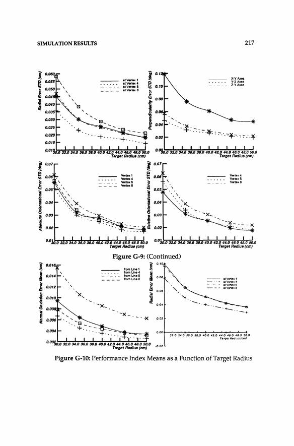
SIMULATION RESULTS
0.03
I ~ O.
~ ! .g a
~ I 0.02 "I:
! J , ! , c: 'x, .g ~ .!!I 0.
~ 0.006 i 0.004
I --_I ~ Vel .. , _5
~ Vel .. 8
! .g a
~ !
I
- .....
X-YAx .. Y-ZAx" Z-V Axel
217
"-l:---.. -. -* : :-.'. -:-liC - - _ • -lIl T···· .. ·T
Vertex 4 VertexS Vertex 8
Figure G-9: (Continued)
lromUn.1 fromUne' from UnaS from Una 8
-x-.-.'X 0.02
liVen •• 1 atV&r1e •• .IVerI.IS ItV",e.,8
o.oot--'--.............. --'-+-....... - .......... --''--...
-0.02
32.0 340 36.0 38.0 "00 42.0 ..... 0 .cG 0 48.0 50.0 T.rset Redlus (em)
Figure G-10: Performance Index Means as a Function of Target Radius

218 SIMULATION RESULTS
I 0.1 I 0.1
I -, j 0.11 V_4 V_4
II _5
1 V_5
ali _8 Vertex a
I I '. ,
I I ~ -! 1 D.H i 00:
Figure G-10: (Continued)

REFERENCES
[1] Agin, G. J. Fitting Ellipses and General Second-Order Curves. Technical Report CMU-RI-TR-81-5, Robotics Institute, Carnegie
Mellon University, Pittsburgh, PA, July, 1981.
[2] Ball, R. S. The Theory of Screws. Cambridge University Press, Cambridge, MA, 1900.
[3] Ballard, D. H. and Brown, C. M. Computer Vision. Prentice Hall, Englewood Cliffs, NJ, 1982.
[4] Chen, J., Wang, C. B., and Yang, C. S. Robot Positioning Accuracy Improvement through Kinematic
Parameter Identification. In the Proceedings of the Third Canadian CAD/CAM in Robotics
Conference, pages 4.7-4.12. June, 1984. Toronto, Canada.
[5] Denavit, J. and Hartenberg, R. S. A Kinematic Notation for Lower-Pair Mechanisms Based on Matrices. Journal of Applied Mechanics 77(2):215-221, June, 1955.
[6] Duda, R. O. and Hart, P. E. Pattern Classification and Scene Analysis. John Wiley and Sons, New York, 1973.
[7] Goldenberg, A. A., Benhabib, B., and Fenton, R. G. A Complete Generalized Solution to the Inverse Kinematics of Robots. Journal of Robotics and Automation RA-1(l):14-20, March, 1985.
[8] Hayati, S. and Mirmirani, M. Puma 600 Robot Arm Geometric Calibration. In The First IEEE International Conference on Robotics. March 13, 1984. Atlanta, GA.

220 REFERENCES
[9] Henrici, P. Essentials of Numerical Analysis, with Pocket Calculator Demonstrations. John Wiley and Sons, New York, 1982.
[10] Isaacson, E. and Keller, J. B. Analysis of Numerical Methods. John Wiley and Sons, New York, 1966.
[11] Kernighan, B. W. and Ritchie, D. M. The C Programming Language. Prentice-Hall, Englewood Cliffs, NJ, 1978.
[12] Khosla, P. K., Neuman, C. P., and Prinz, F. B. An Algorithm for Seam Tracking Applications. The International Journal of Robotic: Research 4(1):27-41, Spring, 1985.
[13] Kirchner, H. O. K., Gurumoorthy, B., and Prinz, F. B. A Perturbation Approach to Robot Calibration. Technical Report CMU-RI-TR-85-9, Robotics Institute, Camegie
Mellon University, Pittsburgh, PA, April, 1985.
[14] Mooring, B. W. The Effect of Joint Axis Misalignment on Robot Positioning Accuracy. In the Proceedings of the International Computers in Engineering
Conference, pages 151-155. ASME, New York, August, 1983. Chicago, IL.
[15] Mooring, B. W. and Tang, G. R. An Improved Method for Identifying the Kinematic Parameters in a
Six Axis Robot. In the Proceedings of the International Computers in Engineering
Conference, pages 79-84. ASME, New York, August, 1984. Las Vegas, NV.
[16] Motorola Incorporated. MC68020 32 Bit Microprocessor User's Manual Prentice Hall, Englewood Cliffs, NJ, 1985.
[17] Motorola Incorporated. MC68881 Floating-Point Coprocessor User's Manual Prentice Hall, Englewood Cliffs, NJ, 1985.
[18] Paul, R. P. Robot Manipulators: Mathematics, Programming, and Control. The MIT Press, Cambridge, MA, 1981.

REFERENCES 221
[19] Paul, R. P., Shima no, S., and Mayer, G. E. Kinematic Control Equations for Simple Manipulators. IEEE Transactions on Systems, Man, and Cybernetics SMC-11(6):449-455,
June, 1981.
[20] Pieper, D. L. The Kinematics of Manipulators under Computer Control. Artifical Intelligence Laboratory Memo AIM-72, Department of Com
puter Science, Stanford University, Stanford, CA, 1968.
[21] Ranky, P. G. Test Method and Software for Robot Qualification. The Industrial Robot 11(2):111-115, June, 1984.
[22J GP-8-3D Sonic Digitizer Operator's Manual Science Accessories Corporation, Southport, CN, 1985.
[23J Stauffer, R. N. Robot Accuracy. Robotics Today 7(2):43-49, April, 1985.
[24J Strang, G. Linear Algebra and Its Applications. Academic Press, New York, 1980.
[25J Sugimoto, K. and Duffy, J. Application of Linear Algebra to Screw Systems. Mechanism and Machine Theory 17(1):73-83, 1982.
[26J Suh, C. and Radcliffe, C. W. Kinematics and Mechanism Design. John Wiley and Sons, New York, 1978.
[27] Unimate Puma Mark II 500 Series Equipment Manual 398U1 Unimation Incorporated, Danbury, CN, 1985.
[28J Val II Programming Language Unimation Incorporated, Danbury, CN, 1985.
[29] Weisberg, S., Applied Linear Regression. John Wiley and Sons, New York, 1980.

222 REFERENCES
[30} Whitney, D. E. and Lozinski, C. A Industrial Robot Calibration Methods and Results. In the Proceedings of the International Computers in Engineering
Conference, pages 92-100. ASME, New York, August, 1984. Las Vegas, NV.
[31} Whitney, D. E., DeFazio, T. L., Gustavson, R. E., Rourke, J. M., Seltzer, D. 5., Edsall, A c., Lozinski, C. A, and Kenwood, G. J. Short-Term and Long-Term Robot Feedback: Multi-Axis Sensing,
Control and Updating. In the Proceedings of the Eleventh Conference on Production Research and
Technology, pages 147-152. Carnegie-Mellon University, Pittsburgh, PA, May, 1984.
[32} Wu, C. The Kinematic Error Model for the Design of Robot Manipulators. In the Proceedings of the American Control Conference, pages 497-502.
San Francisco, CA, June, 1983.

Index
Absolute Orientational Errors 149 Accuracy 177 Assembly Errors 163,175,208
Backlash 19
Backward Multiplication Technique 26 Ball, R. S. 17
Calibration - Sensor 193 Calibration Rods 193 Cartesian Coordinates 81
Cathetometer 114 Center-of-Rotation 44, 176
Center-of-Rotation Estimation 59 Chen 21 Compliance 19 Computational Complexity 90 Control 25 Convergence 88
Convergence Angle 121
Denavit, J. 7 Denavit-Hartenberg Model 10,176 Denavit-Hartenberg Parameters 10,71
Denavit-Hartenberg Zero Configuration 14 Design Model Control 150 Displacement Matrix 17 Displacement Matrix Model 17
Duffy,J. 17
Encoder Calibration Errors 153,160,205 Encoder Resolution 19
Error Propagation 154 Euler Angles 81
Feature Estimate Accuracy 129 Feature Generation 106
Feature Identification 46,47 Fixed Point 84
Forward Kinematics 185 Friction 20
Gear Transmission Error 21 General Transformation Matrix 31
Goldenberg 81 GP-8-3D Sonic Digitizer 98, 102, 194
Grid Touching 111
Hartenberg, R. S. 7 Henrici 86
Henrici, P. 84 Homogeneous Transformation Matrix 7
Identification 21,45 Identified Arm Signatures 120, 191 Inverse Kinematics 79, 186
Jacobi Iterative Algorithm 79, 83, 190
Khosla, Pradeep K. 79 Kinematic Control 25,79,175
Kinematic Features 44 Kinematic Identification 21,43,175
Kinematic Modeling 175 Kinematic Performance 147 Kirchner 21
Line Perpendicularity Errors 150 Line-of-Translation 44,65,176
Linear Displacement Errors 149 Link Coordinate Frames 46, 67 Link Deformation 19
Lozinski, C. A. 15
Machining Errors 163,175,208

224
Manufacturing Error Model 199 Manufacturing Errors 175
Modified Denavit-Hartenberg Model 37 Monte-CarloSimulation 130,147,178
Mooring, B. W. 17
Mooring, Ben 14,21
Newton-Raphson Algorithm 79,80,189
Normal Deviation Errors 149
Number of Measurements 167,213
One-Dimensional Grid Touching 111, 112, 132
Open-Loop Control 79
Orientational Errors 153
Paul, R. P. 7 Paul, Richard 81
Pieper, D. L. 7
Plane-of-Rotation 44, 176
Plane-of-Rotation Estimation 49
Positional Errors 153
Primative Transformations 183
Principal Axis Method 65 Prototype System 97,177
Puma 560 120,185
Radcliffe, C. W. 17
Radial Displacement Errors 149
Ranky Sensor Jig 117 Relative Orientational Errors 150
Roll-Pitch-Yaw 15,81
RotateX 183
RotateY 183
RotateZ 183
RPY 15
S-Model 31,176
S-Model Identification 45
S-Model Parameters 38,46, 70
Screws 17
Sensor Coordinate Frame 104
Sensor Array 98,104
Sensor Calibra tion 193
Sensor Measurement Errors 165,211
Sensor Plane 103
Sensor System 101 Signature Configuration 67,107
Signature Control 79
Signature-Based Control 154 Simulation 199,205
INDEX
Slant Range Compensation 105,194
Slant Ranges 98
Sonic Digi tizer 102
Sugimoto, K. 17
Suh, C. 17
Target Radius 106,169,216
Theory of Screws 17
Three-Dimensional Grid Touching 111, 117, 138
Time-of-Flight 101
Translate X 183
Translate Y 183
Translate Z 183
Two-Dimensional Grid Touching 111,115,135
V AX 11 /780 98
Whitney, D. E. 15
Whitney, Daniel 14,21
Whitney-Lozinski Model 15
Wobble 19
Zero Configuration 14, 17