kinematic and elastostatic design optimisation of the 3 ... · kinematic and elastostatic design...

Modeling, Identification and Control, Vol. 30, No. 2, 2009, pp. 39–56, ISSN 1890–1328

Kinematic and Elastostatic Design Optimisation ofthe 3-DOF Gantry-Tau Parallel Kinematic

Manipulator

Ilya Tyapin 1 Geir Hovland 2

1School of Information Technology and Electrical Engineering, The University of Queensland, Brisbane, Queens-land, 4001, Australia. E-mail: [email protected]

2Department of Engineering, Mechatronics Group, University of Agder, N-4898 Grimstad, Norway. E-mail:[email protected]

Abstract

One of the main advantages of the Gantry-Tau machine is a large accessible workspace/footprint ratiocompared to many other parallel machines. The Gantry-Tau improves this ration further by allowing achange of assembly mode without internal link collisions or collisions between the links and end-effector.The reconfigurable Gantry-Tau kinematic design obtained by multi-objective optimisation according tothis paper gives the following features: 3-D workspace/footprint ratio is more than 3.19, lowest Cartesianstiffness in the workspace is 5N/µm and no link collisions detected. The optimisation parameters arethe support frame lengths, the actuator positions and the robot’s arm lengths. The results comparisonbetween the evolutionary complex search algorithm and gradient-based method used for the Gantry-Taudesign in the past is also presented in this paper. The detailed statics model analysis of the Gantry-Taubased on a functionally dependency is presented in this paper for the first time. Both the statics model andcomplex search algorithm may be applied for other 3-DOF Hexapods without major changes. The existinglab prototype of the Gantry-Tau was assembled and completed at the University of Agder, Norway.

Keywords: parallel manipulator, statics, design optimisation.

1 Introduction

A generalised parallel kinematic manipulator (PKM)is a closed-loop kinematic chain mechanism where theend-effector is linked to the base by several indepen-dent kinematic chains, (Merlet, 2000). It may consistof redundant mechanisms with more actuators than thenumber of controlled degrees of freedom of the end-effector. The study of PKMs has been an active re-search field in robotics and mechanical design for along time and different parallel mechanism with speci-fied number and type of DOF have been proposed. Inthe late 1980s a new field of applications and researchwas developed by (Clavel, 1988), who put the focus on

lower mobility parallel mechanism. The Delta robotpresented by Clavel was a base for a large range ofmachines dedicated to high-speed applications but be-cause of small workspace in relation to footprint andlimited number of degrees of freedom the robot cannot be used as a general purpose manipulator. Pier-rot proposed a 6-DOF fully-parallel robot HEXA. TheHEXA robot, (Pierrot et al., 1992) and (Uchiyamaet al., 1990), is an extension of the Delta mechanismhaving 6 DOFs but because the workspace/footprintratio and tilting angles are small this robot has also alimited capability compared to serial manipulators.

The Tau family of parallel kinematic manipulatorswas invented by ABB Robotics, see (Brog̊ardh, 2000).

doi:10.4173/mic.2009.2.1 c© 2009 Norwegian Society of Automatic Control

http://dx.doi.org/10.4173/mic.2009.2.1

Modeling, Identification and Control

Figure 1: A variant of 3-2-1 link structure mounted onthree quide ways.

The Gantry-Tau PKM makes use of the non-symmetricTau structure that is based on clustering the linksmounted on the actuated arms in the configuration 3-2-1. The different possibilities of Tau structures are pre-sented in (Brog̊ardh and Gu, 2002). The link structure3-2-1 is shown in Fig. 1, where the six links supportonly axial forces. Tool forces (represented by Fh) inthe figure, generate forces and torques on the manip-ulated platform (in the figure a shaft), which are fullysupported by axial forces in the six links. The linkstructure 3-2-1 gives the best opportunities to adaptthe PKM to the specific application requirements. Thehigh stiffness is obtained by the redundant replacementof the linear actuator M1 and position of the link L1;the distance between links can be increased withoutreducing the workspace, it makes a possibility of re-ducing the link forces, especially with respect to thevertical forces on the TCP. The intended applicationsof the Gantry-Tau are high speed machining operationsrequiring a workspace equal to or larger than a typicalserial-type robot’s, but with higher stiffness. However,the robot can also be designed for very fast materialhandling and assembly or for high precision processessuch as laser cutting, water jet cutting and measure-ment.

1.1 Workspace

In order to calculate the workspace one can employdiscretisation methods, geometrical methods or numer-ical methods. For the discretisation method a grid ofnodes with positions and orientations is defined. Thenthe kinematics is calculated for each node and it is

straightforward to verify whether the kinematics canbe solved and to check if joint limits are reached orlink interference occurs. The discretisation algorithmis simple to implement but has some serious drawbacks.It is expensive in computation time and results are lim-ited to the nodes of the grid. One example of this ap-proach is (Dashy et al., 2002). The most common nu-merical methods are based upon the Newton-Raphsonapproach (Whitney, 1969) and its variants. Using ge-ometrical methods the workspace can be calculated asan intersection of simple geometrical objects, (Merlet,2000), for example spheres. The geometric approachto define the Gantry-Tau maximum workspace is pre-sented in this paper.

1.2 Link Collisions

The distance between two geometric objects (lines, seg-ments of lines, rays, surfaces etc.) is defined as the min-imum distance between two points on these objects.Link collisions occur when the distance between twopoints on the links is less than the sum of radii of theselinks. The links of the manipulator are assumed to becylindrical elements.

The link collisions detection methods were pre-sented in (Eberly, 2001), (Merlet and Daney, 2006)and (Teller, 2008), but all use vector cross-products todefine the closest distance between two line segmentsin 3D plane and no functional analysis of the distancefunction in 2D plane was attempted in either (Eberly,2001) and (Teller, 2008). The Gantry-Tau link colli-sions detection presented in (Tyapin, 2009) is based onthe conditional equations (boundaries) search methodand included into the design optimisation scheme pre-sented in this paper. The functional dependency anal-ysis is applied to the condition equations.

1.3 Stiffness

The stiffness is the most important performance spec-ification of parallel kinematic machines. Diment-berg (Dimentberg, 1965) was among the first to usescrew theory to define the stiffness matrix of springsystems in unloaded equilibrium. A stiffness matrixrelates external forces and torques to the linear and an-gular displacements of the joints in the Cartesian space.Since then, the Cartesian stiffness was studied andthere are a lot of calculation methods and algorithmsavailable such as Finite Element Analysis (Pashkevichet al., 2005), virtual joint method (Majou et al., 2004).The stiffness maps of the workspace through JacobianMatrix was established in (Gosselin, 1999), (Bi et al.,2007). The stiffness in X-, Y - and Z-directions werecomputed in (El-Khasawneh and Ferreira, 1999), wherethe minimum and maximum stiffness and directions in

40

Tyapin and Hovland, “Design Optimisation of the 3-DOF Gantry-Tau PKM”

a given configuration were found through the eigenvec-tors analysis. An approach to get the stiffness model ofa tripod-based PKM was presented in (Huang and Mei,2001), where the machine structure is decomposed intotwo substructures: machine frame and parallel mecha-nism.

Two other interesting works considered in our studyare (Li et al., 2002) and (Li and Kao, 2004). The au-thors proposed the conservative congruence transfor-mation (CCT), which represents the stiffness controlbetween the linear Cartesian space at the end-effectorand joint space of a robotic manipulator. In addi-tion, the CCT for the stiffness mapping between thecylindrical space and joint space was presented in (Liet al., 2002) and Jacobian matrix was used to definethe Cartesian stiffness. In (Li and Kao, 2004) CCTwas used to define a kinematic solution for redundantmanipulators. Note that in (Li and Kao, 2004) a newstiffness matrix Kg is defined, which represents thechanges in geometry through the differential Jacobianmatrix, and externally applied forces. In Section 4 ofthis paper, the Kg matrix is not taken into account,since the joint stiffness Kθ dominates for small externalforces.

The closest methods to this paper are presentedin (Pashkevich et al., 2007), (Company et al., 2005)and (Liu et al., 2007). The analytical stiffness mod-elling is presented in (Company et al., 2005), where themethod is based on classical mechanical tools and equa-tions. The application of this method to lower mobilityparallel mechanisms is more difficult than the one forHexapods. For the method in (Company et al., 2005)forces and torques are applied on the endpoint. An-other method is presented in (Pashkevich et al., 2007),where the Jacobian matrices and numerical calcula-tions were used to define the stiffness. In addition, thedesign optimisation is presented in (Pashkevich et al.,2007). The stiffness functional dependency analysis isnot presented in (Pashkevich et al., 2007), (Companyet al., 2005) and (Liu et al., 2007). The randomised op-timal design of PKMs based on control random searchtechnique is presented in Lou et al. (2008), where theeffective regular workspace is introduced. The maindrawback of the method in Lou et al. (2008) is the useof stiffness as the dexterity constraint but not the ob-jective and one objective function based on workspaceis used in Lou et al. (2008). The drawback of the op-timisation algorithm is a lack of ability to reach theglobal optimum if the user is not experienced in thedesign optimisation and can not setup a range of theparameter’s limits. However, the method is good forthe Delta-type PKMs.

Three different approaches to define the Cartesianstiffness of the triangular version of the Gantry-Tau

were used before in (Brog̊ardh et al., 2005), (Williamset al., 2006) and (Hovland et al., 2007). The firstmethod was based on the forward kinematics. Theforward kinematics was required to be calculated innumerical form, but numerical solutions are computa-tionally expensive. The second method was to use theJacobian matrix derived from the inverse kinematicsand matrix inversion. The second method is less com-putational expensive than the first. The third methodwas to use the static matrix and avoid matrix inver-sions to calculate the Cartesian stiffness in (Hovlandet al., 2007). The method presented in this paper isbased on the geometric algebra and functional depen-dency analysis to calculate the static matrix and is anextension of the work in (Hovland et al., 2007). Themain benefit of the static analysis presented in this pa-per is the savings in computational effort. The stiffnessanalysis is developed for the Gantry-Tau but may beused for the other Hexapods with minor changes.

1.4 Multi-Objective Optimisation

The design optimisation may have many objectiveswhich cannot be found numerically and it is a rea-son why most proposed optimal design procedures arefocused on the optimisation of the main characteris-tic of the manipulator, for example, workspace, con-ditioning and stiffness indices, vibration analysis andmanipulability criteria. In Stamper et al. (1997) it isstated that a parallel manipulator with maximum pos-sible workspace may have undesirable characteristicssuch as low stiffness or resonance frequencies, whichmeans that a multi-objective optimisation is needed.The multi-objective design optimisation problem is ex-pressed as follows.

min [ f1(p) , ..., fk(p), fk+1(p) ]

subject to

gi(p) ≤ 0 (1 ≤ i ≤ r)hj(p) = 0 (1 ≤ j ≤ s)pLn ≤ pn ≤ pUn (1 ≤ n ≤ m) (1)

where k is the number of objective functions fk(p), p isa vector of m optimisation parameters, gi(p) and hj(p)are each of the r inequality and s equality problem con-straints, pL and pU are lower and upper limits of theoptimisation parameters. The constraints are consid-ered as a new objective constraints handling functionfk+1(p). Different constraint handling techniques arepresented in Coello (2002).

The most common approach for the constrains han-dling is the use of penalty functions. When using apenalty function, the constraint evaluation is used topenalise an infeasible solution and feasible solutions

41


are favored by the selection process. However, penaltyfunctions have several drawbacks, for example, theyrequire a careful tuning of the penalty factors that ac-curately estimates the level of penalisation.

The complex search method was used for the me-chanical design optimisation in Hansen et al. (2004)and Hansen and Andersen (2001). In Hansen and An-dersen (2001) a mechanical design optimisation of ahydraulically actuated manipulator is presented. Themain objective is minimising the energy consumptionwith side constraints on stability, response time andload dependency. The initial population has 30 de-signs and optimum design is found in 250 iterations.In Hansen et al. (2004) a multi-objective design opti-misation of a servo-robot for a pallets handling is pre-sented. The objectives are the cost and speed. Theaccuracy of the tool point, an expected life of the plan-etary gears and the welded structure, vibrations andthermal conditions of the servo motors are the mainside constraints. Discrete design variables originallyhandled by a mapping technique. The optimum designwas found in 50 iterations with an initial population of10.

In multi-objective optimisation, objectives are notcomparable with respect to their magnitude and valueand may conflict, where some objectives can not be in-creased without a decreasing of others. The result of amulti-objective optimisation is a set of trade-off solu-tions which are considered to be suitable for all objec-tives. In this paper the use of the evolutionary complexsearch algorithm for the PKM’s multi-objective designoptimisation is presented. The optimisation schemeincludes the kinematic, elastostatic properties of themachine and constraint handling based on the penali-sation function.

In Section 2 the kinematic description of the 3-DOF Gantry-Tau parallel kinematic machine is pre-sented. In Section 3 the workspace and unreachableareas caused by the collisions between the manipulatedplatform and support frame are presented. In Section 4a geometric description of the Cartesian stiffness is pre-sented. The parabolic functional dependency methodto calculate the Cartesian stiffness in the Y -directionis presented in Section 4.1. The method to define theCartesian stiffness in the Z-direction is presented inSection 4.2. In Section 4.3 the method for the stiff-ness in the X-direction is presented. In Section 5 the3-DOF Gantry-Tau optimisation problem descriptionand complex search algorithm are presented. In Sec-tions 7 and 6 the results, conclusions and the futureresearch directions are presented.

2 Kinematic Description of the3-DOF Gantry-Tau ParallelKinematic Manipulator

The triangular-link version of the Gantry-Tau kine-matic model is illustrated in Figs. 2, 5 and 8. The 3-DOF Gantry-Tau can be manually reconfigured whileavoiding singularities. As for the basic Gantry-Taustructure, each of the 3 parallel arms (lengths L1, L2

and L3) is controlled by a linear actuator with actua-tion variables q1, q2 and q3. The actuators in Fig. 2 arealigned in the direction of the global X-coordinate.

Figure 2: Triangular-link variant of the Gantry-Taushown in the left-handed configuration for alllink clusters.

Figure 3: The manipulated platform of the Gantry-Taurobot.

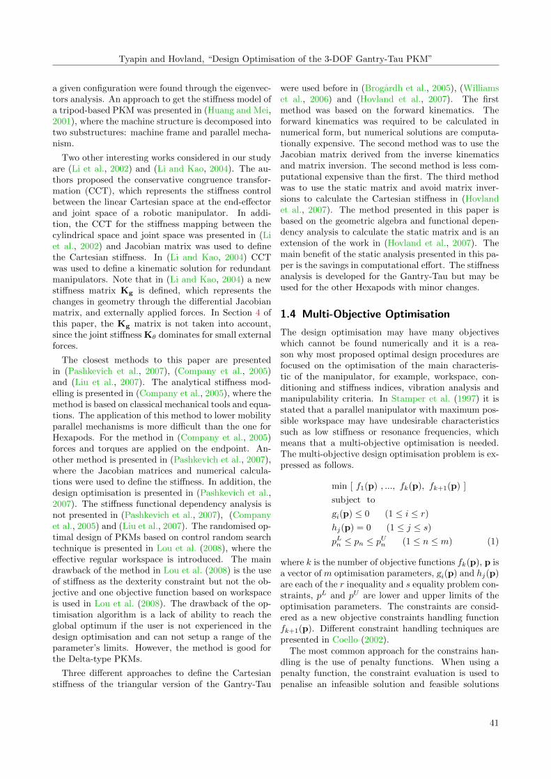
Figs. 3 and 4 show the manipulated platform. Thepoints A, B, C, D, E and F are the link connectionpoints. The arm with one single link connects the actu-ator q1 with platform point F . The arm with two linksconnects actuator q2 with the platform points A andB. The arm with three links connects actuator q3 withthe platform points C, D and E. The triangular pair

42


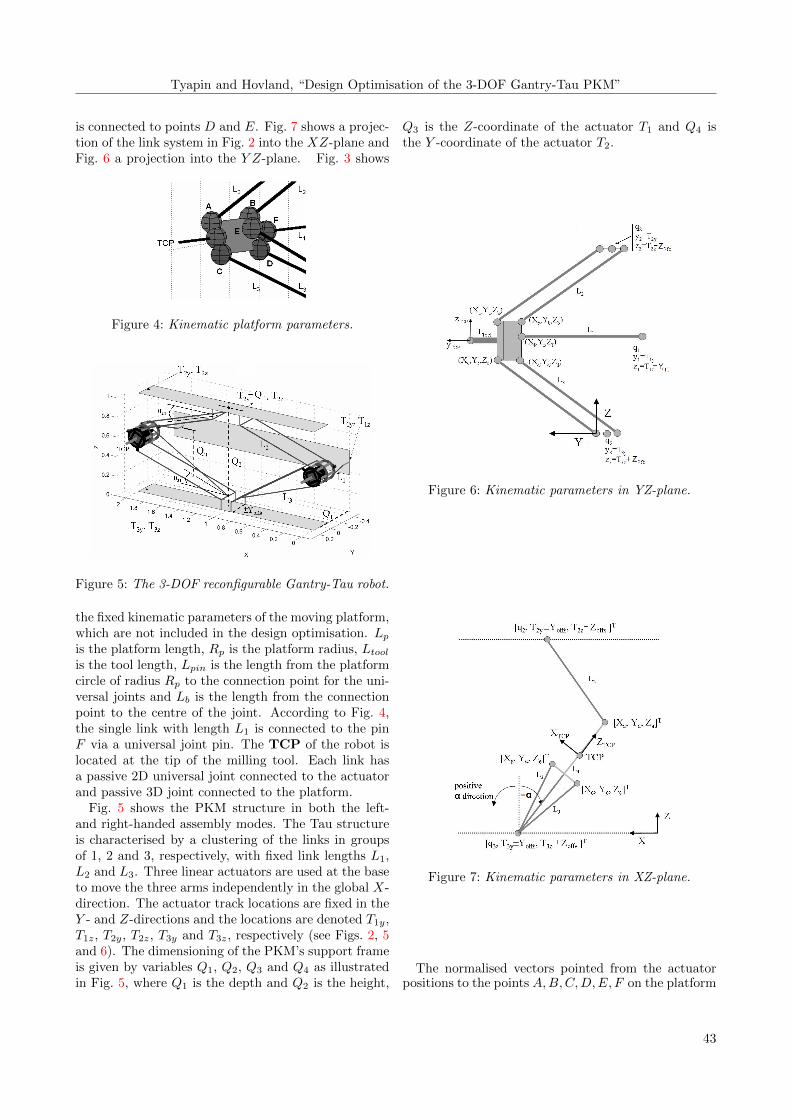
is connected to points D and E. Fig. 7 shows a projec-tion of the link system in Fig. 2 into the XZ-plane andFig. 6 a projection into the Y Z-plane. Fig. 3 shows

Figure 4: Kinematic platform parameters.

Figure 5: The 3-DOF reconfigurable Gantry-Tau robot.

the fixed kinematic parameters of the moving platform,which are not included in the design optimisation. Lpis the platform length, Rp is the platform radius, Ltoolis the tool length, Lpin is the length from the platformcircle of radius Rp to the connection point for the uni-versal joints and Lb is the length from the connectionpoint to the centre of the joint. According to Fig. 4,the single link with length L1 is connected to the pinF via a universal joint pin. The TCP of the robot islocated at the tip of the milling tool. Each link hasa passive 2D universal joint connected to the actuatorand passive 3D joint connected to the platform.

Fig. 5 shows the PKM structure in both the left-and right-handed assembly modes. The Tau structureis characterised by a clustering of the links in groupsof 1, 2 and 3, respectively, with fixed link lengths L1,L2 and L3. Three linear actuators are used at the baseto move the three arms independently in the global X-direction. The actuator track locations are fixed in theY - and Z-directions and the locations are denoted T1y,T1z, T2y, T2z, T3y and T3z, respectively (see Figs. 2, 5and 6). The dimensioning of the PKM’s support frameis given by variables Q1, Q2, Q3 and Q4 as illustratedin Fig. 5, where Q1 is the depth and Q2 is the height,

Q3 is the Z-coordinate of the actuator T1 and Q4 isthe Y -coordinate of the actuator T2.

Figure 6: Kinematic parameters in YZ-plane.

Figure 7: Kinematic parameters in XZ-plane.

The normalised vectors pointed from the actuatorpositions to the points A,B,C,D,E, F on the platform

43


Figure 8: A prototype of the Gantry-Tau with atriangular-mounted link pair built at the Uni-versity of Agder.

Figure 9: Definitions of the variables at the actuatorside for the single link.

are given below.

A = [Ax Ay Az]T B = [Bx By Bz]

T

C = [Cx Cy Cz]T D = [Dx Dy Dz]

T

E = [Ex Ey Ez]T F = [Fx Fy Fz]

T

A = [(axC + azS + dX1) (ay + dY1) (azC − axS + dZ1)]T

B = [(bxC + bzS + dX2) (by + dY2) (bzC − bxS + dZ2)]T

C = [(cxC + czS + dX3) (cy + dY3) (czC − cxS + dZ3)]T

D = [(dxC + dzS + dX4) (dy + dY4) (dzC − dxS + dZ4)]T

E = [(exC + ezS + dX5) (ey + dY5) (ezC − exS + dZ5)]T

F = [(fxC + fzS + dX6) (fy + dY6) (fzC − fxS + dZ6)]T

(2)

where C = cosα, S = sinα, α is the platform ori-entation angle and shown in Fig. 7, dXi = X − Tix,dYi = Y − Tiy, dZi = Z − Tiz, where Tix, Tiy, Tiz arethe coordinates of actuator i for the given TCP posi-

Figure 10: Definitions of the variables at the actuatorside for the double link.

Figure 11: Definitions of the variables at the actuatorside for the triple link.

tions X, Y, Z. [axayaz], [bxbybz], [cxcycz], [dxdydz],[exeyez], [fxfyfz] are the coordinates of the pointsA,B,C,D,E, F in the TCP coordinate frame.

The cosα and sinα equations are given below:

cosα =T3z − Z√

L23m − (Y +My − T3y)2 +

√M2x +M2

z

(3)

sinα =√

1− cos2 α (4)

L3m is the middle length of the triangular-mountedarm 3. M

′

x,M′

y,M′

z are coordinates of a vector from a

midpoint M′

between the triangular link coordinatesC and E on the platform to the actuator position(T3xT3yT3z).

M′

x = Cx +Ex − Cx

2M′

y = Ey M′

z = Cz +Ez − Cz

2

In Figs. 9 - 11 the variables used to define the armmounting on the carts are shown. The drawing to theleft shows the linear actuator variable q1 and the twopassive joint coordinates q1f and q2f for arm 1. In themiddle of the figure, the linear actuator variable q2 isdefined together with the passive joint coordinates q1a,q1b, q2a and q2b for the parallelogram of arm 2. Becauseof the parallelogram, the passive angles are related as

44


follows: q1a = q1b and q2a = q2b. The drawing to theright shows for arm 3 the linear actuator variable q3,the triangular mounted links and the link in parallelwith the plane formed by the triangular links. Becauseof the construction of this arm, the passive joint anglesare related (for a nominal model) as follows: q1c =q1d = q1e and q2c = q2d = q2e. The subscripts a to frefer to the platform connection points A to F , whichare defined in Fig. 4.

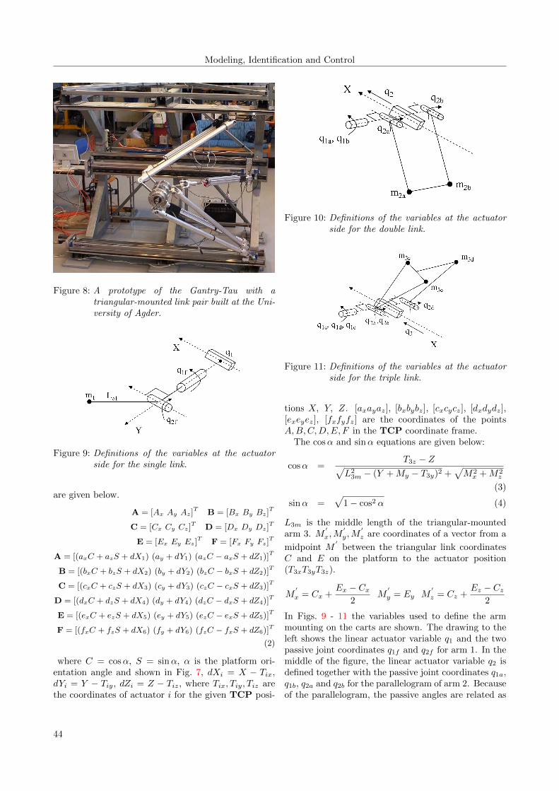
A prototype of the 3-DOF Gantry-Tau with atriangular-mounted link pair built at the University ofAgder, Norway is shown in Fig. 8. The kinematic pa-rameters of the prototype are given below.

Ltool = 0.001 m Lpin = 0.028 m Lb = 0.03 m

Rp = 0.088 m Lp = 0.250 m Yoffs = 0.125 m

L1 = 1 m L2 = 1 m L3 = 1 m Q3 = 0.42 m

Zoffs = 0 Q1 = 0.5m Q2 = 1m Q4 = 0

T1y = −Q1 T1z = Q1 T2y = 0

T2z = Q2 T3y = 0 T3z = 0

T ′1y = T2y + Yoffs T ′1z = T2z − Zoffs

T ′3y = T3y + Yoffs T ′3z = T3z + Zoffs

T ′5y = T3y T ′5z = T3z + Zoffs

T ′2y = T2y − Yoffs T ′2z = T2z − Zoffs

T ′4y = T3y − Yoffs T ′4z = T3z + Zoffs

T ′6y = T1y + Zoffs T ′6z = T1z − Yoffs (5)

where Yoffs and Zoffs are distances from the baseplate to the universal joint in Y - and Z-axis, Tiy Tizare arm actuator positions and T ′iy T

′iz are link actua-

tor positions. X-coordinates of the actuator positionsq1, q2, q3 are defined from general inverse kinematics.

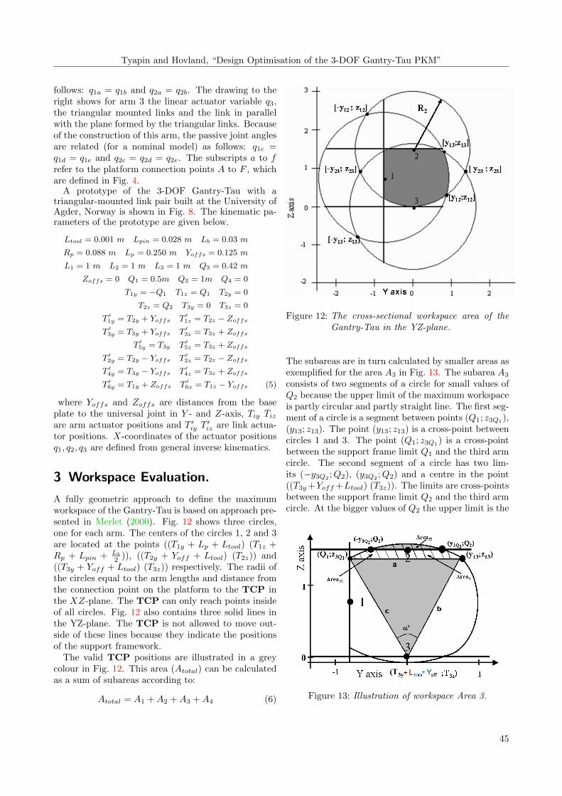
3 Workspace Evaluation.

A fully geometric approach to define the maximumworkspace of the Gantry-Tau is based on approach pre-sented in Merlet (2000). Fig. 12 shows three circles,one for each arm. The centers of the circles 1, 2 and 3are located at the points ((T1y + Lp + Ltool) (T1z +Rp + Lpin + Lb

2 )), ((T2y + Yoff + Ltool) (T2z)) and((T3y + Yoff + Ltool) (T3z)) respectively. The radii ofthe circles equal to the arm lengths and distance fromthe connection point on the platform to the TCP inthe XZ-plane. The TCP can only reach points insideof all circles. Fig. 12 also contains three solid lines inthe YZ-plane. The TCP is not allowed to move out-side of these lines because they indicate the positionsof the support framework.

The valid TCP positions are illustrated in a greycolour in Fig. 12. This area (Atotal) can be calculatedas a sum of subareas according to:

Atotal = A1 +A2 +A3 +A4 (6)

Figure 12: The cross-sectional workspace area of theGantry-Tau in the YZ-plane.

The subareas are in turn calculated by smaller areas asexemplified for the area A3 in Fig. 13. The subarea A3

consists of two segments of a circle for small values ofQ2 because the upper limit of the maximum workspaceis partly circular and partly straight line. The first seg-ment of a circle is a segment between points (Q1; z3Q1

),(y13; z13). The point (y13; z13) is a cross-point betweencircles 1 and 3. The point (Q1; z3Q1

) is a cross-pointbetween the support frame limit Q1 and the third armcircle. The second segment of a circle has two lim-its (−y3Q2

;Q2), (y3Q2;Q2) and a centre in the point

((T3y+Yoff +Ltool) (T3z)). The limits are cross-pointsbetween the support frame limit Q2 and the third armcircle. At the bigger values of Q2 the upper limit is the

Figure 13: Illustration of workspace Area 3.

45


Figure 14: The workspace area of Gantry-Tau machinein the XZ-plane when it is reconfigured towork in both right- and left-handed assemblymodes.

Figure 15: Illustration of the areas where the collisionsbetween the platform and support frame aredetected (grey areas). Square in the middleis the user’s specified workspace.

circle arc between the points (Q1; z3Q1) and (y13; z13).Fig. 14 shows the workspace in the XZ-plane, whichcan be divided into three sections, sections 1 and 3 areoutside of the guide ways and section 2 is between theguide ways.

The collisions between the support frame and ma-nipulated platform reduce the maximum workspace. InFig. 15 the square in the middle defines the user’s spec-ified workspace, where all user’s requirements are met.The areas where the collisions occur are shown in agrey colour. The lengths of these areas ha1, ha2, ha3

and total area AU are expressed as follows.

AU = AU1(ha1) +AU2(ha2) +AU3(ha3) (7)

ha1 = Lp + Ltool (8)

ha2 = R∗p cos(αmin) (9)

ha3 = (

√L2

3 −R∗2p sin2(2π

3) +R∗p cos(

2π

3))R∗p sin(

2π3)

L3

(10)

αmin =π

2− arcsin(

Q2

den) if (Q2 < den) (11)

αmin = 0 if Q2 ≥ den (12)

den =

√L2

3 −R∗2p sin2(2π

3) +R∗p sin(

2π

3) +R∗p (13)

R∗p = Lpin +Rp +Lb2

(14)

where αmin is a minimum possible platform orienta-tion angle for the current design. The first area AU1

is located near the actuator T1 and found as a sum-mary of three geometric objects. The first object isa segment of a circle between points (Q1; z3Q1) and(y1p; z1p). The point (y1p; z1p) is a cross-point be-tween the line y = Q1 − ha1 and circle 3 of the max-imum workspace. The second segment is found be-tween points (Q1; z2Q1) and (y1p;−z1p), where the sec-ond point is a cross-point between circle 2 and liney = Q1 − ha1. The third object (rectangle) is foundbetween points (Q1; z3Q1

), (y1p; z1p), (y1p;−z1p) and(Q1; z2Q1

). Areas AU2 and AU3 are found in a similarway. For more details about the workspace evaluation,link collisions and collisions between the platform andsupport frame refer to Tyapin (2009).

4 Static Analysis.

Figure 16: The Cartesian stiffness in the X-directionas function of the Y- and Z-coordinates.

Let α, β, γ be the TCP orientation angles, li andFi (i = 1, ..., 6) the six PKM link lengths and linkforces. Fx, Fy and Fz are the external Cartesian forces

46


Figure 17: The Cartesian stiffness in the Y-directionas function of the Y- and Z-coordinates.

Figure 18: The Cartesian stiffness in the Z-direction asfunction of the Y- and Z-coordinates.

acting on the TCP. Mx, My and Mz are the externalCartesian torques acting on the TCP. The followingvectors can then be introduced:

X = [X Y Z]T θ = [α β γ]T

F = [Fx Fy Fz]T M = [Mx My Mz]

T

L = [l1 l2 l3 l4 l5 l6]T Fa = [F1 F2 F3 F4 F5 F6]T

The relationship between the TCP forces and the linkforces are.

F =

6∑i=1

Fiui M =

6∑i=1

FiAi × ui (15)

where ui is a unit vector in the direction of link i andAi is a vector pointing from the TCP to the end-pointof link i on the platform. The two equations above canbe rewritten using the 6× 6 statics matrix H.[

FM

]= HFa

[∆X∆θ

]= J∆L (16)

The Jacobian matrix of the PKM relates changesin Cartesian position ∆X and orientation ∆θ withchanges in the link lengths ∆L as shown in Eq. (16)

Figure 19: The Cartesian torsional stiffness in the X-direction as function of the Y- and Z-coordinates.

Figure 20: The Cartesian torsional stiffness in the Y-direction as function of the Y- and Z-coordinates.

(right). In (Gosselin, 1990) the duality between thestatics and the link Jacobian for PKMs is presented,ie.

H−1 = JT

Based on the duality result, the Cartesian stiffness ma-trix K can be derived as a function of the statics matrixas follows.[

FM

]= K

[∆X∆θ

]= HFa = HKL∆L

= HKLJ−1[

∆X∆θ

]= HKLHT

[∆X∆θ

]⇒ K = HKLHT (17)

where KL is a 6×6 diagonal matrix with the individuallink stiffnesses along the diagonal. The matrix KL

is presented in (Hovland et al., 2008). The result inEq. (17) has the benefit that no matrix inversions arerequired to calculate the Cartesian stiffness at X-, Y -and Z-coordinates, including coordinates where H issingular.

47


Figure 21: The Cartesian torsional stiffness in the Z-direction as function of the Y- and Z-coordinates.

Figure 22: Cartesian stiffness in the Y-direction asfunction of the Y-coordinate at fixed X=1.0and Z=0.4.

The elements of the matrix H are the X-, Y - and Z-components of the vectors pointing from the actuatorpositions to the points A,B,C,D,E, F on the platformand X-, Y - and Z- components of the cross-productsof these vectors and vectors pointed from the TCP tothe points A,B,C,D,E, F on the platform, see Fig. 4.The 6× 6 static matrix H is given below.

H =

Ax ... FxAy ... FyAz ... Fz

(A× a)x ... (F× f)x(A× a)y ... (F× f)y(A× a)z ... (F× f)z

(18)

The Y Z functional dependency is applied to find theelements of the static matrix H. Note, that the squaresof the elements are required for the Cartesian stiffness.

Stage 1. In this stage all constants are found. Theconstants are coordinates of the points A...F on theplatform in the TCP coordinate frame, Y - and Z-coordinates of the actuators and link lengths. All these

Figure 23: Cartesian stiffness in the Y-direction asfunction of the Z-coordinate at fixed Y=0.0and X=1.0.

Figure 24: Cartesian stiffness in the Z-direction asfunction of the Y-coordinate at fixed X=1.0and Z=0.3, 0.5, 0.7.

constants are the same for the different Y Z-coordinatesof the TCP.

Stage 2. In this stage Y -coordinate is fixed and Z-coordinate is variable. The upper limit of Z-coordinatedepends on the support frame parameter Q1 and thelower limit is 0. In this paper a calculation algorithmfor the first column of the static matrix is presented.The other 5 columns are found in the same way. Ac-cording to Eqs. (2) and (18),

H11 =ax cosα+ az sinα+X − T ′1x

L2(19)

H21 = ay + Y − T ′1y =C∗∗1a + Y

L2(20)

H31 =az cosα− ax sinα+ Z − T ′1z

L2(21)

where ay, T ′1y, az, ax, T ′1z are constants, C∗∗1a = ay−T ′1yis constant. Index a shows the constants related to thepoint A on the platform. The angle α is expressed as

48


Figure 25: Cartesian stiffness in the Z-direction asfunction of the Z-coordinate at fixed X=1.0and Y=-0.3, 0, 0.3, 0.6.

Figure 26: Cartesian stiffness in the X-direction asfunction of the Y-coordinate at fixed X=1.0and Z=0.3, 0.5, 0.7.

follows.

cosα =T3z − Z√

C′1Y

2 + C′2Y + C

′3

(22)

where C′

1, C′

2, C′

3 are help constants found from Eq. (3).For the fixed Y Eq. (22) is rewritten as follows.

cosα =T3z − Z√

C′′1

sinα =

√1− (T3z − Z)2

C′′1

(23)

According to Eqs. (21) and (23), the element H31 isexpressed as follows.

H31 =az

T3z−Z√C′′1

− ax√

1− (T3z−Z)2

C′′1

+ Z − T ′1zL2

⇒

H31 = C∗∗2a + C∗∗3aZ + C∗∗4a

√C′′2 Z

2 + C′′3 Z + C

′′4

(24)

Figure 27: Cartesian stiffness in the X-direction asfunction of the Z-coordinate at fixed X=1.0and Y=-0.3, 0, 0.3, 0.6.

where

C∗∗2a =T3zaz√C′′1 L2

− T ′1zL2

C∗∗3a = − az√C′′1 L2

+1

L2

C∗∗4a = − axL2

C′′

2 , C′′

3 , C′′

4 are help variables found from Eq. (23).

X − T ′1x =√L22 − (Y − T ′1y)2 − (Z − T ′1z)2 (25)

X − T ′1x =√C′′4aZ

2 + C′′5aZ + C

′′6a (26)

According to Eqs. (23) and (19) the element H11 ofthe static matrix H is given below.

H11 = C∗∗5a + C∗∗6aZ + C∗∗7a

√C′′2 Z

2 + C′′3 Z + C

′′4 +

+√C′′4aZ

2 + C′′5aZ + C

′′6a (27)

C′′

6a =L22 − (Y − T ′1y)2 − T ′21z

L2C′′

5a =2T ′1zL2

C′′

4a =1

L2C∗∗5a =

T3zax√C′′1 L2

C∗∗6a =ax√C′′1 L2

C∗∗7a =azL2

where a simplification for X − T ′1x is given below.

X − T ′1x =√L22 − (Y − T ′1y)2 − (Z − T ′1z)2 (28)

X − T ′1x =√C′′4aZ

2 + C′′5aZ + C

′′6a (29)

Stage 3. In this stage Z-coordinate is fixed and Y -coordinate is variable. The equations for the cosα isexpressed as follows.

cosα =C′′′

1√C′1Y

2 + C′2Y + C

′3

(30)

49


According to Eqs. (21) and (30) an equation for theelement H31 is expresses as follows.

H31 = azC′′′

1

L2

√C′1Y

2 + C′2Y + C

′3

+Z − T ′1zL2

−

− axL2

√1− C

′′′21

C′1Y

2 + C′2Y + C

′3

(31)

H31 =C∗∗∗2a√

C′1Y

2 + C′2Y + C

′3

+ C∗∗∗6a −

−

√C∗∗∗3a Y 2 + C∗∗∗4a Y + C∗∗∗5a

C′1Y

2 + C′2Y + C

′3

(32)

where

C∗∗∗2a =C′′′

1 azL2

C∗∗∗3a =a2xC

′

1

L22

C∗∗∗4a =a2xC

′

2

L22

C∗∗∗5a =a2x(C

′

3 − C′′′2

1 )

L22

C∗∗∗6a =Z − T ′1zL22

According to Eqs. (18) and (2)

H11 =ax cosα+ az sinα+X − T ′1x

L2(33)

X − T ′1x =√L22 − (Y − T ′1y)2 − (Z − T ′1z)2 (34)

X − T ′1x =√C′′′2aY

2 + C′′′3aY + C

′′′4a (35)

The element H11 of the static matrix H is given below.

H11 =C∗∗∗7a√

C′1Y

2 + C′2Y + C

′3

−

−

√C∗∗∗8a Y 2 + C∗∗∗9a Y + C∗∗∗10a

C′1Y

2 + C′2Y + C

′3

+

+√C′′′2aY

2 + C′′′3aY + C

′′′4a (36)

C′′′

4a =L22 − (Z − T ′1z)2 − T

′21y

L22

C′′′

3a =2T ′1yL22

C′′′

2a =1

L22

C∗∗∗7a =C′′′

1 axL2

C∗∗∗8a =a2zC

′

1

L22

C∗∗∗9a =a2zC

′

2

L22

C∗∗∗10a =a2zC

′

3

L22

Stages 4. In this stages the elements H41, H51, H61 ofthe static matrix H are found from the previous stagesas a multiplication of two functional dependencies andnot presented in this paper because of a limited spaceand long equations.

The Cartesian stiffness matrix K is a 6x6 matrix,where the elements k1,1,k2,2 and k3,3 are the stiffnessin the CartesianX-, Y - and Z-directions as functions of

the Y - and Z-coordinates at fixed X-coordinate. Thediagonal elements of the matrix K are given below.

k1,1 = k1H211 + k2H

212 + k3H

213 + k4H

214 + k5H

215 + k6H

216

(37)

k2,2 = k1H221 + k2H

222 + k3H

223 + k4H

224 + k5H

225 + k6H

226

(38)

k3,3 = k1H231 + k2H

232 + k3H

233 + k4H

234 + k5H

235 + k6H

236

(39)

k4,4 = k1H241 + k2H

242 + k3H

243 + k4H

244 + k5H

245 + k6H

246

(40)

k5,5 = k1H251 + k2H

252 + k3H

253 + k4H

254 + k5H

255 + k6H

256

(41)

k6,6 = k1H261 + k2H

262 + k3H

263 + k4H

264 + k5H

265 + k6H

266

(42)

where ki are elements of the matrix KL. The Carte-sian stiffness in the X-, Y -, Z-directions are shown inFigs. 16, 17 and 18. The Cartesian torsional stiffnessare shown in Figs. 19, 20 and 21.

4.1 The Cartesian Stiffness in theY-Direction.

The weakest stiffness for the Gantry-Tau is the stiffnessin the Y -direction when the single link is mounted asin Fig. 8. Increasing the stiffness in the Y -direction isone of the priorities of the stiffness optimisation for theGantry-Tau. The Cartesian stiffness in the Y -directionas a function of the Y -coordinate at fixed X = 1.0 andZ = 0.4 is shown in Fig. 22. The stiffness in the Y -direction are given in Eq. (38). According to Eq. (20),the general equation for the function k2,2 is given be-low.

k2,2 = C∗∗1 Y 2 + C∗∗2 Y + C∗∗3 (43)

C∗∗1 = k1 + k2 + k3 + k4 + k5 + k6

C∗∗2 = k12C∗∗1a + k22C∗∗1b + k32C∗∗1c + k42C∗∗1d +

+k52C∗∗1e + k62C∗∗1f

C∗∗3 = k1C∗∗21a + k2C

∗∗21b + k3C

∗∗21c + k4C

∗∗21d +

+k5C∗∗21e + k6C

∗∗21f

where C∗∗1 , C∗∗2 , C∗∗3 are constants. Eq. (43) is a gen-eral parabolic equation.

The approach presented in this Section reduces acomputation time effort because the stiffness in the Y -direction is found as a parabolic function, where theconstants are calculated before the optimisation starts.The Cartesian stiffness in the Y -direction as a func-tion of the Z-coordinate at fixed Y = 0.0 and X = 1.0is shown in Fig. 23. The stiffness function k2,2(Z) isconstant. The stiffness optimisation process requires amaximisation of the minimum stiffness in a given di-rection. The minimum of the stiffness k2,2(Y ) is found

50


from Eq. (43) and expressed as follows.

k2,2min=

4C∗∗1 C∗∗3 − C∗∗22

4C∗∗1(44)

4.2 The Cartesian Stiffness in theZ-Direction.

The Cartesian stiffness in the Z-direction as a func-tion of the Y -coordinate at fixed X = 1.0 and Z =0.3, 0.5, 0.7 is shown in Fig. 24. The Cartesian stiffnessin the Z-direction as a function of the Z-coordinate atfixed X = 1.0 and Y = −0.3, 0, 0.3, 0.6 is shown inFig. 25.

According to Eqs. (24) and (39), the general equa-tion for the function k3,3 is given below.

k3,3 = C∗∗22 + C∗∗23 Z2 + 2C∗∗2 C∗∗3 Z +

+C∗∗24 (C′′

2 Z2 + C

′′

3 Z + C′′

4 ) +

+2C∗∗2 C∗∗4

√C′′2 Z

2 + C′′3 Z + C

′′4 +

+2C∗∗3 Z√C′′2 Z

2 + C′′3 Z + C

′′4 (45)

where C∗∗2 − C∗∗4 are constants for the given TCPY -coordinate. Due to the additional functions theparabolic functional analysis is not applicable and theCartesian stiffness function is found as a summationof three functions as shown in Eq. (45). The methodpresented in Eq. (45) is suitable for the full range ofthe platform design.

The first derivative of the Eq. (45) is given below.

dk3,3(Z)

dZ= 2C∗∗23 Z + 2C∗∗2 C∗∗3 + C∗∗24 (2C

′′2 Z + C

′′3 ) +

+C∗∗2 C∗∗4 (2C

′′2 Z + C

′′3 ) + 2C∗∗3 (C

′′2 Z

2 + C′′3 Z + C

′′4 )√

C′′2 Z

2 + C′′3 Z + C

′′4

+C∗∗3 Z(2C

′′2 Z + C

′′3 )√

C′′2 Z

2 + C′′3 Z + C

′′4

(46)

The minimum of the Cartesian stiffness in the Z-direction is found from Eq. (46) where the first deriva-tive equals zero or at the boundary of the region. Anal-ysis of these equations shows that the minimum of thestiffness k3,3 is found at fixed X and at the limits ofthe workspace (user’s specified area) on the Y -axis. Z-

coordinate is found by solvingdk3,3(Z)dZ = 0 and both

Z- and Y -coordinates of the minimum are added to theEq. (45).

4.3 The Cartesian Stiffness in theX-Direction.

The Cartesian stiffness in the X-direction as a func-tion of the Y -coordinate at fixed X = 1.0 and Z =

0.3, 0.5, 0.7 is shown in Fig. 26. The Cartesian stiffnessin the Z-direction as a function of the Z-coordinate atfixed X = 1.0 and Y = −0.3, 0, 0.3, 0.6 is shown inFig. 27 and expressed as follows.

k1,1 = k1L22 + k2L

22 + k3L

23 + k4L

23 + k5L

23 +

+k6L21 − k2,2 − k3,3 (47)

The minimum of the Cartesian stiffness in the X-direction is found as a minimum of Eq. (47). However,the minimum of the stiffness in the X-direction is afunction of Y and Z. Analysis of Eqs. (43) and (45)shows that the minimum of the stiffness is found at thelimits of the user specified workspace in the Y - and Z-directions. The minimum of Eq. (47) occurs when k2,2and k3,3 are maximal. The functional analysis showsthat the Cartesian Stiffness in the Y -direction (k2,2)increases significantly faster than k3,3 decreases. In ad-dition, at the Z limits of the user’s specified workspacek3,3 is maximal. The minimum stiffness in the X-direction is found in four cross-points given by Y andZ limits of the user specified workspace.

4.4 Simulations

Figure 28: Links and joints of the existing Gantry-Tauprototype.

The minimum, maximum and average Cartesianstiffness in the X-, Y - and Z-directions of the Gantry-Tau in the entire workspace and the best 70% of theworkspace are given in Table 1. The physical parame-ters of the Gantry-Tau are given in Table 2.

The links and joints of the working Gantry-Tau pro-totype are shown in Fig. 28. Table 3 shows the compu-tational requirements for the four different approacheson the triangular version of the 3-DOF Gantry-TauPKM. The computing time has been normalised to 1for the fourth approach presented in this paper.

The method based on the functional dependency is8250 times faster than the method based on the nu-merical forward kinematics.

5 3-DOF Gantry-Tau DesignOptimisation

The Gantry-Tau multi-objective design optimisationproblem based on the complex search method is ex-

51


Table 1: Cartesian stiffness (N/µm) of the 3-DOFGantry-Tau in the entire workspace and thebest 70 % of the workspace.

Entire workspace X Y ZMinimum 26.59 2.45 19.02Maximum 82.82 50.90 42.29Average 65.49 13.04 26.32

Best 70 percent workspace X Y ZMinimum 60.56 2.45 21.45Maximum 82.82 50.90 42.29Average 72.76 17.48 28.89

Table 2: The Gantry-Tau physical parameters.

Joint weight 1.0kg

Joint stiffness 50 Nµm

Link weight 1.0kg

Link stiffness 232 Nµm

Platform weight 5.0kg

Young’s modulus 70 ∗ 109 Nm2

pressed as follows.

min F(par) = [ fstif (par) fqual(par) fg(par) ]

(48)

Subject to :

QL4 (par) ≤ Q4 ≤ QU4 (par)

QL3 (par) ≤ Q3 ≤ QU3 (par)

LL3 (par) ≤ L3 ≤ LU3 (par)



QL1 (par) ≤ Q1 ≤ ISdthQL2 (par) ≤ Q2 ≤ IShth

where par is a vector of the optimisation parameters.Each optimisation parameter has its upper and lower

Table 3: Static stiffness computation time for four dif-ferent methods.

Method Stiffness,TimeNumerical forward kinematics 8250

Jacobian matrix J 109.9Static matrix H 16.5

Functional dependency 1

limits. The limits of some parameters depend on oth-ers. A detailed limits analysis is presented in Tyapin(2009).

A vector of the optimisation parameters par is givenbelow and described in Section 2.

par = [ Q1 Q2 Q3 Q4 L1 L2 L3 ]

The user’s specifications included into design optimi-sation are the minimum required Cartesian stiffnesslevel kmin, minimum distance between two robot’slinks L∗C , maximum installation space in the X-, Y -and Z-directions ISlth, ISdth and IShth, joint anglesJA, user’s specified workspace in the Y -direction UWa

and in the Z-direction UWb. The objectives vector Fin Eq. (48) includes workspace, collisions, installationspace, statics performances, user’s specifications andexpressed as follows.

fstif (par) =

{kmin

k2,2min(par)

, if kmin > k2,2min(par)

1 , if kmin ≤ k2,2min(par)

}(49)

fqual(par) =IS

AR(par)−AU (par)−∑NUMi=1

δ2i0.7AC(par)

(50)

fg(par) =

r∑i=1

Gi(par)

(51)

AC(par) =

{1 , if link collisions detected0 , if no link collisions

}(52)

where k2,2min(par) is the Cartesian stiffness levelpresented in Section 4.1, AR(par) is the maximumworkspace presented in Section 3, AU (par) is the un-reachable area caused by the collisions between theplatform and support frame presented in Section 3,AC(par) is the link collision parameter and equals 1if collisions are detected or 0 if there are no collisionsfor the current workspace cell, 0.7 is a parameter of thesensitivity and equals the workspace and user’s spec-ified workspace ratio, δ is the workspace integrationparameter, where the minimum workspace cell equalsδ2, NUM is a number of the workspace cells. IS isthe installation space and depends on the parameterQ4. For the positive Q4 the installation space equalsQ2(Q1 +Q4), for negative Q2Q1.

Increasing the Cartesian stiffness in the Y -directionis the main task of the Gantry-Tau statics optimisation.There are some solutions to increase the stiffness. Thefirst solution is reducing the link lengths while supportframe parameters Q1, Q2 are fixed. The second solu-tion is increasing the parameters Q1, Q2 while the linklengths are fixed. The third solution to increase thestiffness is by shifting the Y -position of the actuators

52


T2 and 3. In this paper the Y -position of actuator T2is variable while the actuator T3 position is fixed. Thefourth solution is a change of the distances betweenthe points A and B or E, C and D on the platformas well as the platform length. The last way to in-crease the stiffness in the Y -direction is to increase Q1

while other parameters are fixed. Note, that the sup-port frame parameter Q1 defines the Y -coordinate ofthe actuator T1. The statics objective in Eq. (49) is aratio between the required and minimum stiffness forthe current design, which indicates the level of the ac-ceptance for the given design.

The quality objective in Eq. (50) includes theworkspace, unreachable area, caused by the platformkinematic parameters, installation space and collisionsdetection. The installation space depends on the sup-port frame parameters. The workspace and unreach-able area are the functions of four support frame pa-rameters, individual link lengths and platform kine-matics. In Eq. (50) the maximum workspace AR isreduced by the unreachable areas AU on its bound-aries and summary of the workspace cells, where thecollisions between the links are detected.

The objective function in Eq. (51) keeps the opti-misation parameters (constraints) inside of the limitsand penalise an infeasible constraints. The constraintshandling method is given below.

gi = 0, if ParLi ≤ Parcuri ≤ ParUi(53)

gi =(

ParLi −Parcuri

ParLi

)2, if Parcuri < ParLi (54)

gi =(

Parcuri −ParUiParUi

)2, if Parcuri > ParUi (55)

where Parcuri is a current volume of the parameter i,ParUi is the upper limit of the parameter i, and ParLiis the lower limit of the parameter i.

The complex search method consists of severalstages:

• Generate the initial population of n designs yn. Asa rule of thumb, the size of the initial populationequals m2, where m is a number of the optimisa-tion parameters.

• Objectives are evaluated and the worse and thebest designs are identified as yj and yk respectivelyin each iteration.

• The centroid of the remaining design is found asyc in each iteration.

• The worst design yj is mirrored through the cen-troid yc and a new design is found.

• If the new mirrored through the centroid designcontinues to be the worst design, it is moved to-wards the current best design more or less strongly

depending on how often this had happened in arow.

In Fig. 29 the implementation of the complex searchmethod is shown, when a new design is found as theworst design mirrored through the centroid. The cen-troid yc and a new design yj new are defined as follows.

yc =

∑ni 6=j yi

n− 1yj new = 1.3(yc − yj) + yc (56)

where n is a number of the designs y and yj is the worstdesign. When a new design is found through the bestdesign, some changes are applied.

yc =

∑ni 6=j yi

n− 1ε =

nn0+nrep−1

n00

n0 + nrep − 1

yj new = 0.5(yj + εyc + (1− ε)yk)

where yk is the best design, n0 is a tuning parameter,normally 4− 5, nrep is a number of iterations in a row,where the design yj has been the worse. Parametersn0 and nrep are used to switch the algorithm betweenthe worse and the best designs to find a new one.

Figure 29: Complex search method. The worst designyj is mirrored through centroid yc.

6 Results

The final optimisation design parameters of the 3-DOFGantry-Tau were found using the complex search algo-rithm and gradient-based function fmincon in inte-grated Matlab optimisation toolbox. The optimisationresults obtained in this paper are summarised in Table4 and compared with original design parameters, worseand average designs.

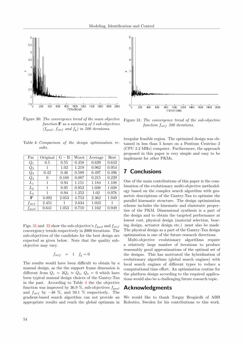
The initial population size is 50 randomised designs.The number of evaluations of the objective functionwas not fixed and optimisation stopped when the dif-ference between the best and worst designs was lessthan 10−3. Fig. 30 shows the convergence trend ofthe main objective function F as a summary of 3sub-objectives (fqual, fstif and fg) in 2000 iterations.

53


Figure 30: The convergence trend of the main objectivefunction F as a summary of 3 sub-objectives(fqual, fstif and fg) in 500 iterations.

Table 4: Comparison of the design optimisation re-sults.

Par Original G− B Worst Average BestQ1 0.5 0.55 0.458 0.639 0.643Q2 1 1.02 1.219 0.962 0.954Q3 0.42 0.46 0.589 0.497 0.496Q4 0 0.168 0.087 0.215 0.229L1 1 0.94 1.151 1.184 1.108L2 1 0.95 0.953 1.038 1.038L3 1 0.94 1.252 1.02 0.976F 3.092 2.053 4.753 2.362 1.949fstif 2.451 1 2.634 1.023 1fqual 0.641 1.053 0.710 1.162 0.949

Figs. 31 and 32 show the sub-objective’s fqual and fstifconvergency trends respectively in 2000 iterations. Thesub-objectives of the candidate for the best design areexpected as given below. Note that the quality sub-objective may vary.

fstif = 1 fg = 0

The results would have been difficult to obtain by amanual design, as the the support frame dimension isdifferent from Q1 = 2Q2 ≈ Q3, Q4 = 0 which havebeen typical manual design choices of the Gantry-Tauin the past. According to Table 4 the the objectivefunction was improved by 36.9 %, sub-objectives fqualand fstif by −48 %, and 59.1 % respectively. Thegradient-based search algorithm can not provide anappropriate results and reach the global optimum in

Figure 31: The convergence trend of the sub-objectivefunction fstif 500 iterations.

irregular feasible region. The optimised design was ob-tained in less than 5 hours on a Pentium Centrino 2(CPU 2.2 MHz) computer. Furthermore, the approachproposed in this paper is very simple and easy to beimplement for other PKMs.

7 Conclusions

One of the main contributions of this paper is the com-bination of the evolutionary multi-objective methodol-ogy based on the complex search algorithm with geo-metric descriptions of the Gantry-Tau to optimise theparallel kinematic structure. The design optimisationscheme includes the kinematic and elaststatic proper-ties of the PKM. Dimensional synthesis is a part ofthe design and to obtain the targeted performance atlowest cost, physical design (material selection, bear-ing design, actuator design etc.) must also be made.The physical design as a part of the Gantry-Tau designoptimisation is one of the future research directions.

Multi-objective evolutionary algorithms requirea relatively large number of iterations to producereasonably good approximations of the optimal set ofthe designs. This has motivated the hybridisation ofevolutionary algorithms (global search engines) withlocal search engines of different types to reduce acomputational time effort. An optimisation routine forthe platform design according to the required applica-tions would also be a challenging future research topic.

Acknowledgments

We would like to thank Torgny Brog̊ardh of ABBRobotics, Sweden for his contributions to this work.

54


Figure 32: The convergence trend of the sub-objectivefunction fqual in 500 iterations.

In addition, we want to acknowledge the support fromthe University of Agder, Norway for providing the re-sources needed to optimise the Gantry-Tau presentedin this paper. The majority of the work presented inthis paper was conducted during the first half of 2008,when I. Tyapin visited the University of Agder.

References

Bi, Z., Lang, S., Zhang, D., Orban, P., and Verner, M.Integrated design toolbox for tripod-based parallelkinematic machines. Journal of Mechanical Design,2007. 129:799–807. doi:10.1115/1.2735340.

Brog̊ardh, T. Design of high performance parallel armrobots for industrial applications. In Proc. of theSymp. Commemorating the Legacy, Works, and Lifeof Sir Robert Stawell Ball Upon the 100th Anniver-sary of A Treatise on the Theory on The Screws.University of Cambridge, Trinity College, 2000 .

Brog̊ardh, T. and Gu, C. Parallel robot development atABB. In Proc. 1st Intl. Coll. of the Collaborative Re-search Centre 562. University of Braunschweig, 2002.

Brog̊ardh, T., Hanssen, S., and Hovland, G.Application-oriented development of parallel kine-matic manipulators with large workspace. In Proc.2nd Intl. Coll. of the Collaborative Research Cen-ter 562:Robotic Systems for Handling and Assembly.Braunschweig, Germany, 2005 pages 153–170.

Clavel, R. Delta, a fast robot with parallel geome-

try. In Intl. Symp. on Industrial Robots. Lausanne,Switzerland, 1988 pages 91–100.

Coello, C. C. Theoretical and numerical constraint-handling techniques used with evolutionary algo-rithms: A survey of the state of the art. Comp.Meth. in Appl. Mech. and Engnrg, 2002. 191((11-12)):1245–1287.

Company, O., Pierrot, F., and Fauroux, J.-C. Amethod for modeling analytical stiffness of a lowermobility parallel manipulator. In IEEE Intl. Conf.on Robotics and Automat. Barcelona, Spain, 2005pages 3232–3237.

Dashy, A., Yeoy, S., Yangz, G., and I.-H.Chery.Workspace analysis and singularity representation ofthree-legged parallel manipulators. In Proc. 7th Intl.Conf. in Control, Automat., Robotics And Vision.Singapore, 2002 pages 962–967.

Dimentberg, F. The screw Calculus and its Applica-tions in Mechanics. Document FTD-HT-23-1632-67,Foreign Technology Division, Wright-Patterson AirForce Base, Ohio, USA, 1965.

Eberly, D. H. 3D game engine design. Morgan Kauf-mann, 2001 page 561.

El-Khasawneh, B. and Ferreira, P. Computation ofstiffness and stiffness bounds for parallel link manip-ulators. In Int. Journal of Machine Tools and Man-ufacture. Elsevier Science Ltd., 1999 pages 321–342.

Gosselin, C. Determination of the workspace of 6-dofparallel manipulators. ASME J. Mech. Des., 1990.112:331–336. doi:10.1115/1.2912612.

Gosselin, C. Stiffness mapping for parallel manipula-tors. IEEE Transactions on Robotics and Automa-tion, 1999. 6(3):377–382. doi:doi:10.1109/70.56657.

Hansen, M. and Andersen, T. A design procedure foractuator control systems using optimization meth-ods. In IEEE The 7th Scandinavian InternationalConference on Fluid Power. 2001 pages 213–221.

Hansen, M., Andersen, T., and Mouritsen, O. Ascheme for handling discrete and continuous designvariables in multi criteria design optimization ofservo mechanisms. In Mechatronics and Robotics.2004 pages 234–245.

Hovland, G., Choux, M., Murray, M., and Brog̊ardh,T. Benchmark of the 3-dof gantry-tau parallel kine-matic machine. In IEEE Intl. Conf. on Robotics andAutomat. Roma, Italy, 2007 pages 535–542.

55

http://dx.doi.org/10.1115/1.2735340

http://dx.doi.org/10.1115/1.2912612

http://dx.doi.org/doi:10.1109/70.56657


Hovland, G., Choux, M., Murray, M., Tyapin, I.,and Brog̊ardh, T. The gantry-tau : Summary oflatest development at ABB, University of Agderand University of Queensland. In 3rd Intl. Collo-quium: Robotic Systems for Handling and Assembly,the Collaborative Research Centre SFB 562. Braun-schweig, Germany, 2008 .

Huang, T. and Mei, J. Stiffness estimation of a tripod-based parallel kinematic machine. In InternationalConference on Robotics and Automation. Seoul, Ko-rea, 2001 pages 3280–3285.

Li, Y., Chen, S.-F., and Kao, I. Stiffness control andtransformation for robotic systems with coordinateand non-coordinate bases. In Intl. Conf. on Roboricsand Automat. Washington, USA, 2002 pages 550–555.

Li, Y. and Kao, I. Stiffness control on redundant ma-nipulators: A unique and kinematically consistentsolution. In Intl. Conf. on Roborics and Automat.New Orleans, USA, 2004 pages 3956–3961.

Liu, H., Ye, C., Wang, H., and Wei, Y. Stiffness anal-ysis and expirement of a parallel kinematic planer.In Proc. of the IEEE International Conference onAutomation and Logistics. Jinan, China, 2007 .

Lou, Y., Liu, G., and Li, Z. Randomized optimal designof parallel manipulators. IEEE Transactions on Au-tomation Science and Engineering, 2008. 5(2):223–233. doi:doi:10.1109/TASE.2007.909446.

Majou, F., Gosselin, C., Wenger, P., and Chablat, D.Parametric stiffness analysis of the orthoglide. InIntl. Symposium on Robotics. 2004 .

Merlet, J.-P. Parallel Robots, page 355. Kluwer Aca-demic Publisher, Solid Mechanics and its Applica-tions, Vol. 74, Dordrecht, Boston, 2000.

Merlet, J.-P. and Daney, D. Leg interference checkingof parallel robots over a given workspace trajectory.In Proc. of the IEEE International Conference onRobotics and Automation. Orlando, Florida, 2006 .

Pashkevich, A., Wenger, P., and Chablat, D. De-sign strategies for the geometric synthesis oforthoglide-type mechanisms. Journal of Mecha-nism and Machine Theory, 2005. 40(8):907–930.doi:10.1016/j.mechmachtheory.2004.12.006.

Pashkevich, A., Wenger, P., and Chablat, D. Kine-matic and stiffness analysis of the Orthoglide, aPKM with simple, regular workspace and homoge-neous performances. In IEEE Intl. Conf. on Roboticsand Automat. Roma, Italy, 2007 pages 549–555.

Pierrot, F., Uchiyama, M., Dauchez, P., and Fournier,A. A new design of a 6-dof parallel robot. In Proc.23rd Intl. Symp. on Industrial Robots. 1992 pages771–776.

Stamper, R., Tsai, L., and Walsh, G. Optimization of athree dof translational platform for well-conditionedworkspace. In Proc. of the Int. Conf. Robotics andAutomation. New Mexico, 1997 pages 3250–3255.

Teller, S. Distance between two line segments in 3D.Geometric tools, http://www.geometrictools.com,1998-2008, 2008 .

Tyapin, I. Multi-objective design optimiation of a classof parallel kinematic machines. In Ph.D Thesis. Bris-bane, Queensland, Australia, 2009 pages 1–266.

Uchiyama, M., Iimura, K., Pierrot, F., Dauchez, P.,Unno, K., and Toyama, O. A new design of a veryfast 6-dof parallel robot. Journal of Robotics andMechatronics, 1990. 2(4):308–315.

Whitney, D. E. Optimum step size control for Newton-Raphson solution of nonlinear vector equations.1969. 14(4):572–574.

Williams, I., Hovland, G., and Brog̊ardh, T. Kinematicerror calibration of the gantry-tau parallel manipu-lator. In IEEE Intl. Conf. on Robotics and Automat.Orlando, 2006 pages 4199–4204.

56

http://dx.doi.org/doi:10.1109/TASE.2007.909446

http://dx.doi.org/10.1016/j.mechmachtheory.2004.12.006

http://creativecommons.org/licenses/by/3.0

kinematic and elastostatic design optimisation of the 3 ... · kinematic and elastostatic design...

Documents