Electro-elastostatic analysis of multiple cracksin an infinitely long piezoelectric strip:a hypersingular integral approach

L. Athanasius, W. T. Ang* and I. SridharSchool of Mechanical and Aerospace Engineering

Nanyang Technological UniversityRepublic of Singapore

Abstract

The problem of an arbitrary number of arbitrarily oriented straightcracks in an infinitely long piezoelectric strip is considered here. Thecracks are acted by suitably prescribed internal tractions and are as-sumed to be either electrically impermeable or permeable. A Green’sfunction which satisfies the conditions on the parallel edges of the stripis derived using a Fourier transform technique and applied to formulatethe electroelastic crack problem in terms of a system of hypersingu-lar integral equations. Once the hypersingular integral equations aresolved, quantities of practical interest, such as the crack tip stress andelectric displacement intensity factors, can be easily computed. Somespecific cases of the problem are examined.

Keywords: electroelasticity, cracks, Green’s function, hypersingularintegral equations

This is a preprint of an article accepted for publication in theEuropean Journal of Mechanics-A/Solids (2010).

* Author for correspondence (W. T. Ang)E-mail: mwtang@ntu.edu.sghttp://www.ntu.edu.sg/home/mwtang/

1

1 Introduction

In recent years, the problem of determining the electro-elastostatic fields

around cracks in an infinitely long piezoelectric strip has been a subject of

considerable interest among many researchers. Most of the works reported in

the literature deal with cracks that have specific geometries and orientations,

such as a single straight crack oriented in a direction that is either parallel

or perpendicular to the edges of the piezoelectric strip.

For mathematical simplicity, many researchers have studied cases in which

the piezoelectric strip is deformed by antiplane shear stress and inplane elec-

trical static loads. For such special cases, Li [6] and Shindo et al [13] applied

a Fourier transform technique to reduce the problem of a straight crack to

solving a Fredholm integral equation, and Li et al [7, 8, 19] derived closed-

form formulae for the electro-elastic field intensity factors and energy release

rates of a pair of collinear cracks. Some other works of related interest in-

clude those of Li and Lee [9] and Kwon and Lee [10] on a straight crack in a

piezoelectric strip of finite length subject to an antiplane deformation.

If the piezoelectric strip is deformed by inplane mechanical and electrical

loads, the problem is more complicated to solve. Particular plane problems

involving piezoelectric strips with relatively simple crack configurations were

solved by Shindo et al [14] and Wang et al [15—18].

The present paper considers the problem of an infinitely long piezoelectric

strip containing an arbitrary number of arbitrarily oriented straight cracks

under mixed mode electro-elastostatic loads. The cracks are assumed to be

either electrically impermeable or permeable. The solution approach here is

to construct an appropriate Green’s function for the governing equations of

linear electroelasticity and use it to reduce the problem under consideration

to solving hypersingular integral equations which describe the conditions on

2

the cracks. The Green’s function which satisfies prescribed conditions on

the edges of the piezoelectric strip is derived with aid of exponential Fourier

transformation. Once the hypersingular integral equations are solved, physi-

cal quantities of interest such as the crack tip stress and electric displacement

intensity factors can be readily computed. The analysis presented here covers

both inplane and antiplane deformations and their coupling. It is applied to

solve some specific cases of the problem under consideration.

Figure 1. A sketch of the problem on the Ox1x2 plane.

2 The problem

With reference to an Ox1x2x3 Cartesian coordinate system, consider an in-

finitely long piezoelectric strip −∞ < x1 <∞, 0 < x2 < h, −∞ < x3 <∞,where h is a given positive constant. The strip contains N arbitrarily ori-

ented straight cracks whose geometries do not change along the x3 axis. The

cracks are denoted by Γ(1), Γ(2), · · · , Γ(N−1) and Γ(N). On the Ox1x2 plane,

3

the tips of the k-th crack Γ(k) are given by (a(k)1 , a

(k)2 ) and (b

(k)1 , b

(k)2 ). Refer to

Figure 1. The cracks do not intersect with one another or the edges x2 = 0

and x2 = h. It is also assumed that the electroelastic deformation of the

cracked piezoelectric strip does not depend on the spatial coordinate x3 and

time.

We are interested in determining the displacements uk(x1, x2) and electric

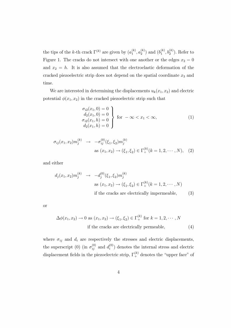
potential φ(x1, x2) in the cracked piezoelectric strip such that

σi2(x1, 0) = 0d2(x1, 0) = 0σi2(x1, h) = 0d2(x1, h) = 0

for −∞ < x1 <∞, (1)

σij(x1, x2)m(k)j → −σ(0)ij (ξ1, ξ2)m(k)

j

as (x1, x2)→ (ξ1, ξ2) ∈ Γ(k)+ (k = 1, 2, · · · , N), (2)

and either

dj(x1, x2)m(k)j → −d(0)j (ξ1, ξ2)m(k)

j

as (x1, x2)→ (ξ1, ξ2) ∈ Γ(k)+ (k = 1, 2, · · · ,N)

if the cracks are electrically impermeable, (3)

or

∆φ(x1, x2)→ 0 as (x1, x2)→ (ξ1, ξ2) ∈ Γ(k)+ for k = 1, 2, · · · , N

if the cracks are electrically permeable, (4)

where σij and di are respectively the stresses and electric displacements,

the superscript (0) (in σ(0)ij and d

(0)i ) denotes the internal stress and electric

displacement fields in the piezoelectric strip, Γ(k)+ denotes the “upper face” of

4

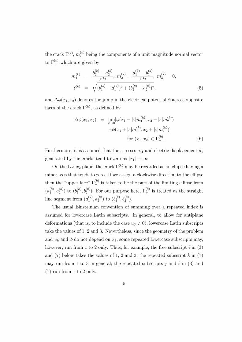
the crack Γ(k), m(k)i being the components of a unit magnitude normal vector

to Γ(k)+ which are given by

m(k)1 =

b(k)2 − a(k)2`(k)

, m(k)2 =

a(k)1 − b(k)1`(k)

, m(k)3 = 0,

`(k) =

q(b(k)1 − a(k)1 )2 + (b(k)2 − a(k)2 )2, (5)

and ∆φ(x1, x2) denotes the jump in the electrical potential φ across opposite

faces of the crack Γ(k), as defined by

∆φ(x1, x2) = limε→0[φ(x1 − |ε|m(k)

1 , x2 − |ε|m(k)2 )

−φ(x1 + |ε|m(k)1 , x2 + |ε|m(k)

2 )]

for (x1, x2) ∈ Γ(k)+ . (6)

Furthermore, it is assumed that the stresses σi1 and electric displacement d1

generated by the cracks tend to zero as |x1|→∞.On the Ox1x2 plane, the crack Γ

(k) may be regarded as an ellipse having a

minor axis that tends to zero. If we assign a clockwise direction to the ellipse

then the “upper face” Γ(k)+ is taken to be the part of the limiting ellipse from

(a(k)1 , a

(k)2 ) to (b

(k)1 , b

(k)2 ). For our purpose here, Γ

(k)+ is treated as the straight

line segment from (a(k)1 , a

(k)2 ) to (b

(k)1 , b

(k)2 ).

The usual Einsteinian convention of summing over a repeated index is

assumed for lowercase Latin subscripts. In general, to allow for antiplane

deformations (that is, to include the case u3 6= 0), lowercase Latin subscriptstake the values of 1, 2 and 3. Nevertheless, since the geometry of the problem

and uk and φ do not depend on x3, some repeated lowercase subscripts may,

however, run from 1 to 2 only. Thus, for example, the free subscript i in (3)

and (7) below takes the values of 1, 2 and 3; the repeated subscript k in (7)

may run from 1 to 3 in general; the repeated subscripts j and ` in (3) and

(7) run from 1 to 2 only.

5

3 Basic equations of electroelasticity

For time independent electroelastic problems, the governing equations for

the displacements uk and electric potential φ in a homogeneous piezoelectric

material are given by

cijk`∂2uk

∂xj∂x`+ e`ij

∂2φ

∂xj∂x`= 0,

ejk`∂2uk

∂xj∂x`− κj`

∂2φ

∂xj∂x`= 0, (7)

where cijk`, e`ij and κi` are the constant elastic moduli, piezoelectric coeffi-

cients and dielectric coefficients respectively.

The constitutive equations relating (σij, dj) and (uk,φ) are

σij = cijk`∂uk∂x`

+ e`ij∂φ

∂x`,

dj = ejk`∂uk∂x`− κjp

∂φ

∂x`. (8)

Following closely the approach of Barnett and Lothe [1], we define

UJ =

½uj for J = j = 1, 2, 3,φ for J = 4,

SIj =

½σij for I = i = 1, 2, 3,dj for I = 4,

CIjK` =

cijk` for I = i = 1, 2, 3 and K = k = 1, 2, 3,e`ij for I = i = 1, 2, 3 and K = 4,ejk` for I = 4 and K = k = 1, 2, 3,−κj` for I = 4 and K = 4,

(9)

so that (7) and (8) may be written more compactly as

CIjK`∂2UK∂xj∂x`

= 0 (I = 1, 2, 3, 4) (10)

6

and

SIj = CIjK`∂UK∂x`

(I = 1, 2, 3, 4; j = 1, 2, 3) (11)

respectively. Note that uppercase Latin subscripts have values 1, 2, 3 and 4.

Summation is also implied for repeated uppercase Latin subscripts running

from 1 to 4. For example, in (11) there is a summation over K from 1 to 4

and a summation over ` from 1 to 2.

Thus, the problem stated in Section 2 can be mathematically posed as

one which requires solving (10) in the region 0 < x2 < h subject to the

conditions

SI2(x1, 0) = 0SI2(x1, h) = 0

¾for −∞ < x1 <∞. (12)

SIj(x1, x2)m(k)j → −S(0)Ij (ξ1, ξ2)m(k)

j

as (x1, x2) → (ξ1, ξ2) ∈ Γ(k)+ (k = 1, 2, · · · , N) for I = 1, 2, 3, (13)

and either

S4j(x1, x2)m(k)j → −S(0)4j (ξ1, ξ2)m(k)

j

as (x1, x2) → (ξ1, ξ2) ∈ Γ(k)+ (k = 1, 2, · · · ,N)

if the cracks are electrically impermeable, (14)

or

∆U4(x1, x2)→ 0 as (x1, x2)→ (ξ1, ξ2) ∈ Γ(k)+ for k = 1, 2, · · · , Nif the cracks are electrically permeable, (15)

where

∆UI(x1, x2) = limε→0[UI(x1 − |ε|m(k)

1 , x2 − |ε|m(k)2 )

−UI(x1 + |ε|m(k)1 , x2 + |ε|m(k)

2 )]

for (x1, x2) ∈ Γ(k)+ . (16)

7

In addition, it is required that SI1 → 0 as |x1|→∞.For the case in which UK are functions of x1 and x2 only, the general

solution of (10) can be written as

UK(x1, x2) = Re4X

α=1

AKαfα(zα), (17)

where Re denotes the real part of a complex number, fα are analytic functions

of zα = x1+ταx2 in the domain of interest, τα are the solutions, with positive

imaginary parts, of the 8-th order polynomial (characteristic) equation

det[CI1K1 + (CI1K2 + CI2K1)τ + CI2K2τ2] = 0 (18)

and AKα are solutions of the homogeneous system

[CI1K1 + (CI1K2 + CI2K1)τα + CI2K2τ2α]AKα = 0. (19)

The characteristic equation (18) admits solutions which occur in pairs of

complex conjugates (Barnett and Lothe [1]).

The generalised stress functions SIj corresponding to (17) are given by

SIj = Re4X

α=1

LIjαf0α(zα), (20)

where the prime denotes differentiation with respect to the relevant argument

and

LIjα = (CIjK1 + ταCIjK2)AKα. (21)

4 Green’s function for a piezoelectric strip

Here we construct a Green’s function ΦKR(x1, x2; ξ1, ξ2) which satisfies the

partial differential equations

CIjK`∂2

∂xj∂x`[ΦKR(x1, x2; ξ1, ξ2)] = δIRδ(x1 − ξ1, x2 − ξ2)

for 0 < x2 < h and 0 < ξ2 < h. (22)

8

and the boundary conditions

ΞI2R(x1, 0; ξ1, ξ2) = 0ΞI2R(x1, h; ξ1, ξ2) = 0

¾for −∞ < x1 <∞, (23)

where δIR is the Kronecker-delta, δ denotes the Dirac-delta function and

ΞIjR(x1, x2; ξ1, ξ2) = CIjK`∂

∂x`[ΦKR(x1, x2; ξ1, ξ2)]. (24)

Guided by the analysis in Clements [3], we take

ΦKR(x1, x2; ξ1, ξ2)

=1

2πRe

4Xα=1

AKαNαS ln(zα − cα)DSR + Φ∗KR(x1, x2; ξ1, ξ2)

for 0 < ξ2 < h, (25)

where

Φ∗KR(x1, x2; ξ1, ξ2)

= − 12πRe

4Xα=1

AKαMαP

4Xβ=1

LP2βNβS ln(zα − cβ)DSR

+1

2π

Z ∞

0

Re4X

α=1

AKαMαP [EPR(u; ξ1, ξ2) exp(iuzα)

−EPR(u; ξ1, ξ2) exp(−iuzα) + FPR(u; ξ1, ξ2)]du, (26)

the overhead bar denotes the complex conjugate of a complex number, i =√−1, EPR(u; ξ1, ξ2) and FPR(u; ξ1, ξ2) are arbitrary functions to be deter-mined, cα = ξ1 + ταξ2, [NαS] is the inverse of [AKα], [MαP ] is the inverse of

[LI2α] and DSR are real constants defined by

4Xα=1

ImLI2αNαSDSR = δIR. (27)

Note that Im denotes the imaginary part of a complex number.

9

From (24), (25) and (26), we obtain

ΞKjR(x1, x2; ξ1, ξ2)

=1

2πRe

4Xα=1

LKjαNαS(zα − cα)−1DSR + Ξ∗KjR(x1, x2; ξ1, ξ2)

for 0 < ξ2 < h, (28)

where

Ξ∗KjR(x1, x2; ξ1, ξ2)

= − 12πRe

4Xα=1

LKjαMαP

4Xβ=1

LP2βNβS(zα − cβ)−1DSR

+1

2π

Z ∞

0

Re4X

α=1

iLKjαMαPu[EPR(u; ξ1, ξ2) exp(iuzα)

+EPR(u; ξ1, ξ2) exp(−iuzα)]du. (29)

It can be shown that (28) and (29) satisfy (22) and the boundary condi-

tions given on the first line in (23). The boundary conditions on the second

line in (23) are fulfilled if

Re4X

α=1

LK2αNαS(x1 + ταh− cα)−1DSR

−Re4X

α=1

LK2αMαP

4Xβ=1

LP2βNβS(x1 + ταh− cβ)−1DSR

+

Z ∞

0

Re4X

α=1

iLK2αMαPu[EPR(u; ξ1, ξ2) exp(iu[x1 + ταh])

+EPR(u; ξ1, ξ2) exp(−iu[x1 + ταh])]du= 0 for −∞ < x1 <∞. (30)

Taking the exponential Fourier transform of both sides of (30) over the

10

interval −∞ < x1 <∞, we find that

u4X

α=1

LK2αMαP exp(iuταh)− LK2αMαP exp(iuταh)EPR(u; ξ1, ξ2)

=4X

α=1

LK2αNαS exp(−iu[cα − ταh])DSR

−4X

α=1

LK2αMαP

4Xβ=1

LP2βNβS exp(−iu[cβ − ταh])DSR. (31)

We can invert (31) as a system of linear algebraic equations to obtain

EPR(u; ξ1, ξ2). The functions EPR(u; ξ1, ξ2) are not well defined at u = 0. It

can be shown that the integrand of the improper integral in (26) is bounded

over the interval 0 < u <∞ if we choose FPR(u; ξ1, ξ2) to be given by

FPR(u; ξ1, ξ2) = EPR(u; ξ1, ξ2)− EPR(u; ξ1, ξ2). (32)

Note that the functions EPR(u; ξ1, ξ2) tend to zero as the width h tends

to infinity (that is, for a piezoelectric half-space x2 > 0).

5 Hypersingular integral formulation

Let Ω be the region bounded by a simple closed curve ∂Ω on the Ox1x2

plane. If the functions UK(x1, x2) and ΦKR(x1, x2; ξ1, ξ2) respectively satisfy

(10) and (22) in Ω then it can be shown that

UR(ξ1, ξ2) =

Z∂Ω

[UI(x1, x2)ΞIjR(x1, x2; ξ1, ξ2)

−ΦIR(x1, x2; ξ1, ξ2)SIj(x1, x2)]nj(x1, x2)ds(x1, x2)for (ξ1, ξ2) ∈ Ω, (33)

where [n1(x1, x2), n2(x1, x2)] is the outward unit normal to Ω at the point

(x1, x2) on the boundary ∂Ω and SIj(x1, x2) and ΞIjR(x1, x2; ξ1, ξ2) are de-

11

fined by (11) and (24) respectively. For further details on the boundary

integral equations in (33), refer to Clements [3], Pan [12] and Garcia et al [4].

If we apply (33) together with the Green’s function ΦKR(x1, x2; ξ1, ξ2)

and the corresponding stress function ΞKjR(x1, x2; ξ1, ξ2) as given by (25),

(26), (28), (29) and (31) to the crack problem stated in Section 2, we obtain

UR(ξ1, ξ2) =NXk=1

ZΓ(k)+

∆UI(x1, x2)m(k)p ΞIpR(x1, x2; ξ1, ξ2)ds(x1, x2)

for 0 < ξ2 < h, (34)

where ∆UI(x1, x2) is as defined in (16). In (34), Γ(k)+ (the “upper face” of the

crack Γ(k)) is taken to be the straight line from (a(k)1 , a

(k)2 ) to (b

(k)1 , b

(k)2 ).

The integration in (34) is only over the crack faces. The integrals over

x2 = 0 and x2 = h vanish because of (12) and (23). Also, note that the far

field condition that SI1 → 0 as |x1|→ 0 is used in deriving (34).

From (11) and (34), we obtain

SKj(ξ1, ξ2) =NXk=1

ZΓ(k)+

∆UI(x1, x2)CKjR`m(k)p

× ∂

∂ξ`[ΞIpR(x1, x2; ξ1, ξ2)]ds(x1, x2)

for 0 < ξ2 < h. (35)

Conditions on the cracks given by (13) and either (14) (for electrically

impermeable cracks) or (15) (for electrically permeable cracks) can be used

to derive a system of hypersingular integral equations containing the un-

known functions ∆UI(x1, x2) for (x1, x2) ∈ Γ(k)+ (k = 1, 2, · · · , N). The

unknown functions can be determined by solving numerically the system of

hypersingular integral equations.

12

5.1 Electrically impermeable cracks

For electrically impermeable cracks, the system of hypersingular integral

equations derived from (13) and (14) is given by

H+1Z−1

χ(q)IK∆U

(q)I (v)

(t− v)2 dv +NXn=1n6=q

+1Z−1

∆U(n)I (v)Λ

(nq)IK (v, t)dv

+NXn=1

+1Z−1

∆U(n)I (v)Ψ

(nq)IK (v, t)dv = −S(0)Kj(X(q)

1 (t), X(q)2 (t))m

(q)j

for − 1 < t < 1, K = 1, 2, 3, 4 and q = 1, 2, · · · , N , (36)

where H denotes that the integral is to be interpreted in the Hadamard

finite-part sense and

∆U(q)I (v) = ∆UI(X

(q)1 (v), X

(q)2 (v)),

Λ(nq)IK (v, t) =

1

4πRe

4Xα=1

QIKrjαm(n)j m

(q)r `(n)

([X(n)1 (v)−X(q)

1 (t)] + τα[X(n)2 (v)−X(q)

2 (t)])2,

Ψ(nq)IK (v, t) =

m(n)j m

(q)r `(n)

4πRe

Z ∞

0

4Xα=1

iuLIjαMαP

×[CKrRs ∂

∂ξs(EPR(u; ξ1, ξ2)) exp(iuZ

(n)α (v))

+CKrRs∂

∂ξs(EPR(u; ξ1, ξ2)) exp(−iuZ(n)α (v))]du

−4X

α=1

LIjαMαP

4Xβ=1

BPKrβ

× 1

([X(n)1 (v)−X(q)

1 (t)] + ταX(n)2 (v)− τβX

(q)2 (t))

2,

13

X(q)1 (v) =

(b(q)1 + a

(q)1 )

2+(b(q)1 − a(q)1 )2

v,

X(q)2 (v) =

(b(q)2 + a

(q)2 )

2+(b(q)2 − a(q)2 )2

v,

Z(q)α (v) = X(q)1 (v) + ταX

(q)2 (v),

χ(q)IK =

1

πRe

4Xα=1

QIKrjαm(q)j m

(q)r `(q)

([b(q)1 − a(q)1 ] + τα[b

(q)2 − a(q)2 ])2

,

QIKrjα = (CKrR1 + ταCKrR2)TIjαR, TIjαS = LIjαNαRDRS,

BPKrβ = (CKrR1 + τβCKrR2)HPβR, HPβR = LP2βNβSDSR. (37)

The numerical method in Kaya and Erdogan [5] can be used to solve (36)

approximately for ∆U(q)I (v) as follows.

Let

∆U(n)P (v) '

√1− v2

JXj=1

ψ(nj)P U (j−1)(v), (38)

where U (j)(x) = sin([j + 1] arccos(x))/ sin(arccos(x)) is the jth order Cheby-

shev polynomial of the second kind and ψ(nj)P are the constants to be deter-

mined.

Substitution of (38) into (36) yields

−JXj=1

jπψ(qj)I χ

(q)IKU

(j−1)(t)

+NXn=1n6=q

JXj=1

ψ(nj)I

+1Z−1

√1− v2U (j−1)(v)Λ(nq)IK (v, t)dv

+NXn=1

JXj=1

ψ(nj)I

+1Z−1

√1− v2U (j−1)(v)Ψ(nq)

IK (v, t)dv

= −S(0)Kj(X(q)1 (t),X

(q)2 (t))m

(q)j (39)

for − 1 < t < 1, K = 1, 2, 3, 4 and q = 1, 2, · · · ,N.

14

Note that (39) contains 4JN unknown constants ψ(nj)P (P = 1, 2, 3, 4;

n = 1, 2, · · · , N ; j = 1, 2, · · · , J). By letting t = cos([2i − 1]π/[2J ]) fori = 1, 2, · · · , J, we can generate a system of 4JN linear algebraic equations

which can be solved for the unknown constants.

5.2 Electrically permeable cracks

From (15), ∆U(q)4 (v) = 0 for −1 < v < 1 and q = 1, 2, · · · , N, if the

cracks are electrically permeable. According to (13), the unknown functions

∆U(q)1 (v), ∆U

(q)2 (v) and ∆U

(q)3 (v) are governed by (36) (with ∆U

(q)4 (v) = 0)

for K = 1, 2, 3 (instead of K = 1, 2, 3, 4). The functions ∆U(q)1 (v), ∆U

(q)2 (v)

and ∆U(q)3 (v) can be approximated using (38) and the unknown constants

ψ(nj)1 , ψ(nj)2 and ψ(nj)3 are given by (39) with ψ(nj)4 = 0 for K = 1, 2, 3 (instead

of K = 1, 2, 3, 4). As before, we can let t = cos([2i− 1]π/[2J ]) for i = 1, 2,· · · , J, to generate a system of 3JN linear algebraic equations to solve for

the unknowns.

6 Stress and electric displacement intensity

factors

For the specific problems considered below in Section 7, we calculate the

stress and electric displacement intensity factors at the tips (a(n)1 , a

(n)2 ) and

(b(n)1 , b

(n)2 ) of the n-th crack Γ(n) defined as follows:

KI(a(n)1 , a

(n)2 ) = lim

t→−1−

r`(n)

2

p−2(t+ 1)(S1j(X(n)

1 (t), X(n)2 (t))m

(n)1

+S2j(X(n)1 (t),X

(n)2 (t))m

(n)2 )m

(n)j ,

KII(a(n)1 , a

(n)2 ) = lim

t→−1−

r`(n)

2

p−2(t+ 1)(S1j(X(n)

1 (t), X(n)2 (t))m

(n)2

−S2j(X(n)1 (t), X

(n)2 (t))m

(n)1 )m

(n)j ,

15

KIII(a(n)1 , a

(n)2 ) = lim

t→−1−

r`(n)

2

p−2(t+ 1)S3j(X(n)

1 (t), X(n)2 (t))m

(n)j ,

KIV (a(n)1 , a

(n)2 ) = lim

t→−1−

r`(n)

2

p−2(t+ 1)S4j(X(n)

1 (t), X(n)2 (t))m

(n)j ,

KI(b(n)1 , b

(n)2 ) = lim

t→1+

r`(n)

2

p2(t− 1)(S1j(X(n)

1 (t), X(n)2 (t))m

(n)1

+S2j(X(n)1 (t), X

(n)2 (t))m

(n)2 )m

(n)j ,

KII(b(n)1 , b

(n)2 ) = lim

t→1+

r`(n)

2

p2(t− 1)(S1j(X(n)

1 (t), X(n)2 (t))m

(n)2

−S2j(X(n)1 (t),X

(n)2 (t))m

(n)1 )m

(n)j ,

KIII(b(n)1 , b

(n)2 ) = lim

t→1+

r`(n)

2

p2(t− 1)S3j(X(n)

1 (t), X(n)2 (t))m

(n)j ,

KIV (b(n)1 , b

(n)2 ) = lim

t→1+

r`(n)

2

p2(t− 1)S4j(X(n)

1 (t), X(n)2 (t))m(n)

j . (40)

Using (35) and (38), we find that (40) gives

KI(a(n)1 , a

(n)2 ) '

r`(n)

2π(χ

(n)P1m

(n)1 + χ

(n)P2m

(n)2 )

JXj=1

ψ(nj)P U (j−1)(−1)

KII(a(n)1 , a

(n)2 ) '

r`(n)

2π(χ

(n)P1m

(n)2 − χ

(n)P2m

(n)1 )

JXj=1

ψ(nj)P U (j−1)(−1),

KIII(a(n)1 , a

(n)2 ) ' −

r`(n)

2πχ

(n)P3

JXj=1

ψ(nj)P U (j−1)(−1)

KIV (a(n)1 , a

(n)2 ) ' −

r`(n)

2πχ

(n)P4

JXj=1

ψ(nj)P U (j−1)(−1)

KI(b(n)1 , b

(n)2 ) '

r`(n)

2π(χ(n)P1m

(n)1 + χ(n)P2m

(n)2 )

JXj=1

ψ(nj)P U (j−1)(+1)

KII(b(n)1 , b

(n)2 ) '

r`(n)

2π(χ

(n)P1m

(n)2 − χ

(n)P2m

(n)1 )

JXj=1

ψ(nj)P U (j−1)(+1),

16

KIII(b(n)1 , b

(n)2 ) ' −

r`(n)

2πχ

(n)P3

JXj=1

ψ(nj)P U (j−1)(+1)

KIV (b(n)1 , b

(n)2 ) ' −

r`(n)

2πχ(n)P4

JXj=1

ψ(nj)P U (j−1)(+1). (41)

7 Specific cases

Some specific cases of the electroelastic crack problem stated in Section 2 are

solved here using the analysis presented in Section 5.

Figure 2. A horizontal electrically impermeable crack in the strip.

Case 1. To check our results against those given in Wang and Noda [18],

we consider the case of a single horizontal straight crack −a < x1 < a, x2 = b,−∞ < x3 <∞, in the infinitely-long piezoelectric strip with electrical polingalong the x2 direction. Note that a > 0 and 0 < b < h.We take the tips of the

crack to be (a(1)1 , a

(1)2 ) = (a, b) and (b

(1)1 , b

(1)2 ) = (−a, b). The crack is assumed

to be electrically impermeable. A geometrical sketch of the problem is given

in Figure 2. In [18], the same problem is formulated in terms of singular

integral equations (that is, by using an approach equivalent to modelling the

crack as a continuous distribution of dislocations).

17

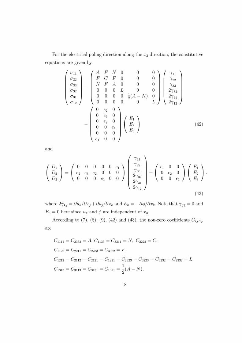
For the electrical poling direction along the x2 direction, the constitutive

equations are given byσ11σ22σ33σ32σ31σ12

=

A F N 0 0 0F C F 0 0 0N F A 0 0 00 0 0 L 0 00 0 0 0 1

2(A−N) 0

0 0 0 0 0 L

γ11γ22γ332γ322γ312γ12

−

0 e2 00 e3 00 e2 00 0 e10 0 0e1 0 0

E1E2E3

(42)

and

D1D2D3

=

0 0 0 0 0 e1e2 e3 e2 0 0 00 0 0 e1 0 0

γ11γ22γ332γ322γ312γ12

+ ²1 0 00 ²2 00 0 ²1

E1E2E3

.(43)

where 2γkj = ∂uk/∂xj+∂uj/∂xk and Ek = −∂φ/∂xk. Note that γ33 = 0 andE3 = 0 here since uk and φ are independent of x3.

According to (7), (8), (9), (42) and (43), the non-zero coefficients CIjKp

are

C1111 = C3333 = A, C1133 = C3311 = N, C2222 = C,

C1122 = C2211 = C2233 = C3322 = F ,

C1212 = C2112 = C2121 = C1221 = C2323 = C3223 = C3232 = C2332 = L,

C1313 = C3113 = C3131 = C1331 =1

2(A−N),

18

C2141 = C1241 = C3243 = C2343 = C4121 = C4112 = C4332 = C4323 = e1,

C1142 = C3342 = C4211 = C4233 = e2,

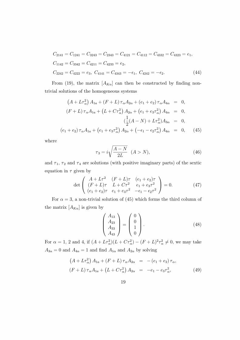
C2242 = C4222 = e3, C4141 = C4343 = −²1, C4242 = −²2. (44)

From (19), the matrix [AKα] can then be constructed by finding non-

trivial solutions of the homogeneous systems¡A+ Lτ 2α

¢A1a + (F + L) ταA2α + (e1 + e2) ταA4α = 0,

(F + L) ταA1a +¡L+ Cτ2α

¢A2α +

¡e1 + e3τ

2α

¢A4α = 0,

(1

2(A−N) + Lτ 2α)A3α = 0,

(e1 + e2) ταA1a +¡e1 + e3τ

2α

¢A2α +

¡−²1 − ²2τ2α¢A4α = 0, (45)

where

τ 3 = i

rA−N2L

(A > N), (46)

and τ 1, τ2 and τ 4 are solutions (with positive imaginary parts) of the sextic

equation in τ given by

det

A+ Lτ 2 (F + L)τ (e1 + e2)τ(F + L)τ L+ Cτ2 e1 + e3τ

2

(e1 + e2)τ e1 + e3τ2 −²1 − ²2τ2

= 0. (47)

For α = 3, a non-trivial solution of (45) which forms the third column of

the matrix [AKα] is given byA13A23A33A43

=

0010

. (48)

For α = 1, 2 and 4, if (A+ Lτ 2α)(L + Cτ2α)− (F + L)2τ2α 6= 0, we may take

A3α = 0 and A4α = 1 and find A1α and A2α by solving¡A+ Lτ2α

¢A1a + (F + L) ταA2α = − (e1 + e2) τα,

(F + L) ταA1a +¡L+ Cτ2α

¢A2α = −e1 − e3τ 2α, (49)

19

in order to construct the first, second and fourth columns of the matrix [AKα].

To compare our results with those in Wang and Noda [18], we use the

following material constants:

A = 12.6× 1010, N = 5.5× 1010, F = 8.41× 1010,C = 11.7× 1010, L = 2.3× 1010,e1 = 17.44, e2 = −6.5, e3 = 23.3,²1 = 150.3× 10−10, ²2 = 130.0× 10−10. (50)

The values of A, N, F , C and L above are in N/m2, e1, e2 and e3 are in

C/m2, and ²1 and ²2 are in C/(Vm).

Figure 3. Plots of KI(a, b)/(σ0√a), CKII(a, b)/(Fσ0

√a) and

CKIV (a, b)/(e3σ0√a) against b/h.

20

Figure 4. Plots of KI(a, b)/(σ0√a) and CKIV (a, b)/(e3σ0

√a) against

CD0/(e3σ0).

In Figure 3, for internal loads on the crack given by S(0)12 = 0, S

(0)22 = σ0,

S(0)32 = 0 and S

(0)42 = 0 (σ0 is a positive constant) and for h/a = 4.0, the

non-dimensionalised crack tip stress intensity factors KI(a, b)/(σ0√a) and

CKII(a, b)/(Fσ0√a) and the non-dimensionalised crack tip electrical dis-

placement intensity factor CKIV (a, b)/(e3σ0√a) are plotted against b/h for

0.10 ≤ b/h ≤ 0.50 and compared with the numerical values given by Wangand Noda in [18]. (Note that KIII(a, b) = 0 for the problem under considera-

tion.) For 0.20 ≤ b/h ≤ 0.50, our plots are almost visually indistinguishableform those obtained using the numerical values of Wang and Noda [18]. For

b/h nearer to 0, there is, however, a small but noticeable difference between

the two sets of values for the intensity factors. Except for b/h smaller than

21

0.20, the numerical values of the intensity factors are observed to converge

to at least 4 significant figures when J in (38) is increased from 5 to 10. For

b/h which is smaller than 0.20, that is, when there is a stronger interaction

between the crack and the edge x2 = 0, convergence to 2 or more significant

figures is observed when we increase J from 10 to 20.

In Figure 4, for the crack under uniform internal loads S(0)12 = 0, S

(0)22 = σ0,

S(0)32 = 0 and S

(0)42 = D0 (σ0 is a positive constant and D0 a non-negative

constant) and for h/a = 4.0 and b/h = 0.50, we plot KI(a, b)/(σ0√a)

and CKIV (a, b)/(e3σ0√a) against the non-dimensionalised electrical load

CD0/(e3σ0) for 0 ≤ CD0/(e3σ0) ≤ 7.0. The plots (obtained using J = 5

in (38)) agree well with the numerical values from Wang and Noda [18].

Case 2. Consider now the case in which the electrical poling is taken to be

along the x3 direction with the constitutive equations given byσ11σ22σ33σ32σ31σ12

=

A N F 0 0 0N A F 0 0 0F F C 0 0 00 0 0 L 0 00 0 0 0 L 00 0 0 0 0 1

2(A−N)

γ11γ22γ332γ322γ312γ12

−

0 0 e20 0 e20 0 e30 e1 0e1 0 00 0 0

E1E2E3

, (51)

22

and

D1D2D3

=

0 0 0 0 e1 00 0 0 e1 0 0e2 e2 e3 0 0 0

γ11γ22γ332γ322γ312γ12

+ ²1 0 00 ²1 00 0 ²2

E1E2E3

.(52)

It follows that the non-zero coefficients CIjKp are

C1111 = A, C2222 = A, C1122 = C2211 = N, C3333 = C,

C1133 = C3311 = C2233 = C3322 = F ,

C1313 = C3113 = C3131 = C1331 = C2323 = C3223 = C3232 = C2332 = L,

C1212 = C2112 = C2121 = C1221 =1

2(A−N),

C3141 = C1341 = C2342 = C3242 = C4131 = C4113 = C4223 = C4232 = e1,

C1143 = C2243 = C4311 = C4322 = e2,

C3343 = C4333 = e3, C4141 = C4242 = −²1, C4343 = −²2. (53)

The homogeneous system in (19) reduces to

(A+1

2(A−N) τ 2α)A1α + (

1

2N +

1

2A)ταA2α = 0,

(1

2N +

1

2A)ταA1α + (

1

2A− 1

2N +Aτ 2α)A2α = 0,¡

L+ Lτ2α¢A3α +

¡e1 + e1τ

2α

¢A4α = 0,¡

e1 + e1τ2α

¢A3α −

¡²1 + ²1τ

2α

¢A4α = 0. (54)

Note that (54) cannot be used to construct [AKα] that is invertible. To

overcome this minor difficulty, a relatively small amount of anisotropy is

introduced into the equations governing u1 and u2. Specifically, we replace

23

C1111 = A in (53) by C1111 = A+ ε, where ε is a selected real number whose

magnitude is very small compared to A. It follows that instead of (54) the

linear algebraic equations for working out AKα are given by

(A+ ε+1

2(A−N) τ 2α)A1α + (

1

2N +

1

2A)ταA2α = 0,

(1

2N +

1

2A)ταA1α + (

1

2A− 1

2N +Aτ 2α)A2α = 0,¡

L+ Lτ2α¢A3α +

¡e1 + e1τ

2α

¢A4α = 0,¡

e1 + e1τ2α

¢A3α +

¡−²1 − ²1τ2α¢A4α = 0. (55)

We can take τ3 = τ4 = i and τ1 and τ2 are two distinct solutions with

positive imaginary parts of the quartic equation

det

µA+ ε+ 1

2(A−N)τ2 (N + 1

2(A−N))τ

(N + 12(A−N))τ 1

2(A−N) +Aτ 2

¶= 0. (56)

Note that (56) cannot yield two distinct solutions with positive imaginary

parts if ε is zero.

From (55), we find that AKa may be chosen to be

A1α = −(N + 1

2(A−N))τα

A+ ε+ 12(A−N)τ 2α

(δα1 + δα2)

A2α = δα1 + δα2, A3α = δα3, A4α = δα4. (57)

The matrix [AKα] as constructed in (57) is invertible if τ1 6= τ 2.

For electrical poling along the x3 direction, we consider the case of two

electrically permeable collinear cracks which are centrally located in the

piezoelectric strip, as studied by Li [7]. Specifically, the cracks lie on the

plane x1 = 0 and their crack tips are given by (a(1)1 , a

(1)2 ) = (0, h/2− d− 2a),

(b(1)1 , b

(1)2 ) = (0, h/2− d), (a(2)1 , a(2)2 ) = (0, h/2 + d) and (b(2)1 , b(2)2 ) = (0, h/2 +

d + 2a), that is, 2a is the length of each of the crack and 2d is the distance

separating the inner crack tips. A geometrical sketch of the problem is given

24

in Figure 5. The electrically permeable cracks are acted upon by uniform

internal loads given by S(0)11 = 0, S

(0)21 = 0 and S

(0)31 = τ0 (τ0 is a positive

constant).

Figure 5. Two electrically permeable collinear cracks centrally located in

the strip.

To obtain some numerical results, the relevant material constants are

taken to be

A = 12.6× 1010, N = 5.5× 1010, F = 5.3× 1010,L = 3.53× 1010, e1 = 17.0, ²1 = 151× 10−10. (58)

The values of C, e2, e3 and ²2 are not given above as they do not play a role

in the computation here.

Using the constants in (58) and J = 5 in (38), we compute the non-

dimensionalised stress intensity factors KIII(0, h/2− d− 2a)/(τ 0√a) (at an

outer tip) and KIII(0, h/2 − d)/(τ 0√a) (at an inner tip) for h/a = 9. In

Figure 6, the non-dimensional stress intensity factors are plotted against d/a

for 0.10 ≤ d/a ≤ 2.40. The values of the stress intensity factors are in goodagreement with those calculated using the analytical formulae given in Li [7].

25

Figure 6. Plots of KIII(0, h/2− d− 2a)/(τ0√a) andKIII(0, h/2− d)/(τ0

√a) against d/a.

Case 3. Consider now three parallel cracks in the infinitely-long piezoelec-

tric strip as sketched in Figure 7. Specifically, the middle crack is of length 2a

and has tips given by (a, h/2) and (−a, h/2). The tips of the crack above themiddle crack are (b, d+ h/2) and (−b, d+ h/2) and those of the crack beloware (b,−d+h/2) and (−b,−d+h/2). The top and bottom cracks have equallength 2b. The uniform internal loads on the electrically impermeable cracks

are given by S(0)12 = 0, S

(0)22 = σ0, S

(0)32 = 0 and S

(0)42 = D0 with D0/σ0 = 10

−10

CN−1 (σ0 and D0 are positive constants). As in Case 1 above, the electrical

poling is in the x2 direction and the material constants of the strip are given

26

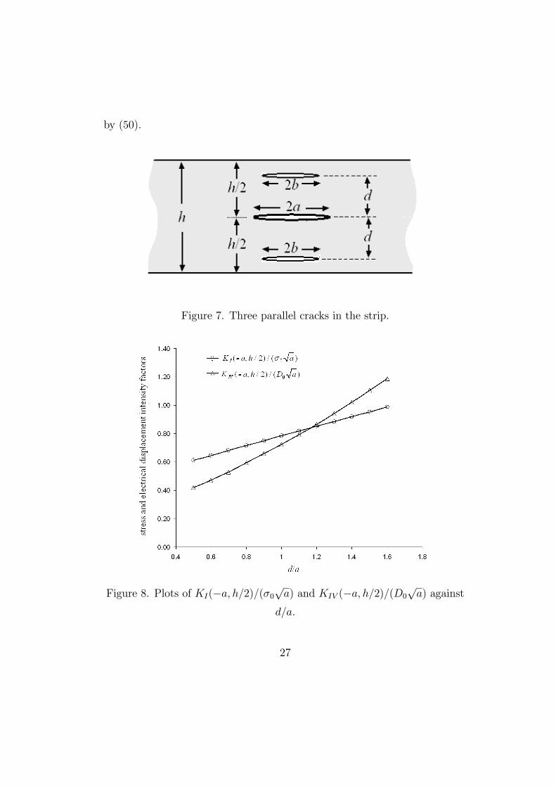
by (50).

Figure 7. Three parallel cracks in the strip.

Figure 8. Plots of KI(−a, h/2)/(σ0√a) and KIV (−a, h/2)/(D0

√a) against

d/a.

27

For h/a = 4 and b/a = 1, plots of the non-dimensionalised stress intensity

factor KI(−a, h/2)/(σ0√a) and the electrical displacement intensity factorKIV (−a, h/2)/(D0

√a) at the tip (−a, h/2) of the middle crack against d/a

for 0.50 ≤ d/a ≤ 1.60 are given in Figure 8.

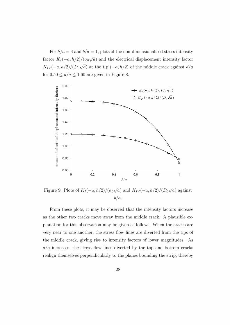
Figure 9. Plots of KI(−a, h/2)/(σ0√a) and KIV (−a, h/2)/(D0

√a) against

b/a.

From these plots, it may be observed that the intensity factors increase

as the other two cracks move away from the middle crack. A plausible ex-

planation for this observation may be given as follows. When the cracks are

very near to one another, the stress flow lines are diverted from the tips of

the middle crack, giving rise to intensity factors of lower magnitudes. As

d/a increases, the stress flow lines diverted by the top and bottom cracks

realign themselves perpendicularly to the planes bounding the strip, thereby

28

interacting more strongly with the tips of the middle crack. It is clear that

the top and bottom cracks have a shielding effect on the middle crack.

The shielding effect can also be observed by altering the half crack length

b of the top and bottom cracks. For h/a = 4 and d/a = 1, the non-

dimensionalised stress intensity factorKI(−a, h/2)/(σ0√a) and the electricaldisplacement intensity factor KIV (−a, h/2)/(D0

√a) at the tip (−a, h/2) of

the middle crack are plotted against b/a for 0 ≤ b/a ≤ 1 in Figure 9. It isobvious that the intensity factors decrease with increasing b/a. Their vari-

ations are quite slow and gradual as b/a increases from 0 to 0.50 and only

start to become more pronounced for b/a > 0.50.

Figure 10. Two inclined cracks and a horizontal crack.

Case 4. Here we study the interaction between two inclined cracks and a

horizontal crack. A geometrical sketch of the problem is given in Figure 10.

Specifically, the horizontal crack lies in the region −a < x1 < a, x2 = h/2,−∞ < x3 < ∞. The tips of the inclined crack on the left are given by(−d+ a cos θ, h/2 + a sin θ) and (−d− a cos θ, h/2− a sin θ) and those of the

29

other inclined crack by (d−a cos θ, h/2+a sin θ) and (d+a cos θ, h/2−a sin θ).The uniform internal loads on the electrically impermeable cracks are given

by S(0)12 = 0, S

(0)22 = σ0, S

(0)32 = 0 and S

(0)42 = D0 with D0/σ0 = 10

−10 CN−1 (σ0

and D0 are positive constants). The electrical poling is in the x2 direction

and the material constants of the strip are given by (50).

Figure 11. Plots of KI(−a, h/2)/(σ0√a) against (d− a)/a.

We examine the effect of the inclined cracks on the mode I stress and elec-

trical displacement intensity factors of the horizontal crack as the distance d

changes. For h/a = 4.0, Figures 11 and 12 give plots of KI(−a, h/2)/(σ0√a)

and KIV (−a, h/2)/(D0√a) respectively against (d − a)/a for 0.50 ≤ (d −a)/a ≤ 3.5 for three different values of the angle θ. As expected, we observethat each of the intensity factors tends to a fixed value for all the three values

of the angle θ, as the distance (d − a)/a increases. For 0 ≤ θ ≤ π/2, the

inclined cracks appear to have a greater influence on the intensity factors of

30

the horizontal crack if the angle θ is smaller. For θ = π/6 and θ = π/3, each

of the intensity factors has a peak value at a particular value of (d− a)/a. Itmay be of some interest to note that the variations of KI(−a, h/2)/(σ0

√a)

with (d− a)/a are qualitatively the same as those of KIV (−a, h/2)/(D0√a).

Figure 12. Plots of KIV (−a, h/2)/(D0√a) against (d− a)/a.

For θ = π/6, KI(−a, h/2)/(σ0√a) is found to be negative when the non-

dimensionalised distance (d−a)/a is smaller than 0.50. This suggests that theinclined cracks may possibly generate a compressive load on the horizontal

crack near its tips. Thus, depending on the angle θ and the distance (d−a)/a,opposite faces of the cracks in Figure 10 may possibly come into contact with

each other near the crack tips. The solution in Section 5 assumes that the

cracks open up completely under the action of suitably prescribed internal

tractions and hence may not be physically valid if crack closure occurs.

31

Figure 13. Plots of KI(−a, h/2)/(σ0√a), KII(−a, h/2)/(σ0

√a) and

KIV (−a, h/2)/(D0√a) against (d− a)/a for θ = π/4.

For either (d−a)/a→∞ or θ = π/2, the mode II crack tip stress intensity

factor of the horizontal crack is zero (since S(0)12 = 0). In general, the presence

of the inclined cracks may, however, cause a mode II deformation at the tips

of the horizontal crack. In Figure 13, for h/a = 4.0 and θ = π/4, the non-

dimensionalised intensity factorsKI(−a, h/2)/(σ0√a), KII(−a, h/2)/(σ0

√a)

and KIV (−a, h/2)/(D0√a) (at the tip (−a, h/2) of the horizontal crack) are

plotted against (d − a)/a for 0.30 ≤ (d − a)/a ≤ 3.5. Note that, as be-

fore, the variation of KI(−a, h/2)/(σ0√a) with (d − a)/a shows the same

qualitative feature as that of KIV (−a, h/2)/(D0√a). For (d− a)/a ≥ 1, the

mode II stress intensity factor KII(−a, h/2)/(σ0√a) is relatively small inmagnitude. The effect of the inclined cracks on KII(−a, h/2)/(σ0

√a) be-

comes more pronounced as the distance (d−a)/a decreases. From Figure 13,

32

it appears that the magnitudes of the intensity factors KI(−a, h/2)/(σ0√a),

KII(−a, h/2)/(σ0√a) andKIV (−a, h/2)/(D0√a) increase rapidly as the cracktip (−a, h/2) of the horizontal crack approaches the inclined cracks.

Case 5. Consider two centrally located parallel cracks of equal length 2a as

sketched in Figure 14. The tips of the first crack are given by (−d, h/2−a) and(−d, h/2+a) and those of the second cracks by (d, h/2−a) and (d, h/2+a).The electrical poling is in the vertical x2 direction. The internal tractions

on the cracks are given by S(0)11 = σ0, S

(0)21 = 0 and S

(0)31 = 0. The cracks are

assumed to be electrically permeable. The influence of the width h of the

strip on the stress and electric displacement intensity factors at the crack

tips is examined here.

Figure 14. Two parallel cracks perpendicular to the strip.

For the case in which the material constants of the strip are given by

(50), numerical values of KI(−d, h/2−a)/(σ0√a), KII(−d, h/2−a)/(σ0√a)and the and CKIV (−d, h/2 − a)/(e3σ0

√a) (non-dimensionalised stress and

electric displacement intensity factors at the crack tip (−d, h/2−a)) are givenin Table 1 for d/a = 0.50 and selected values of h/a. The numerical values of

33

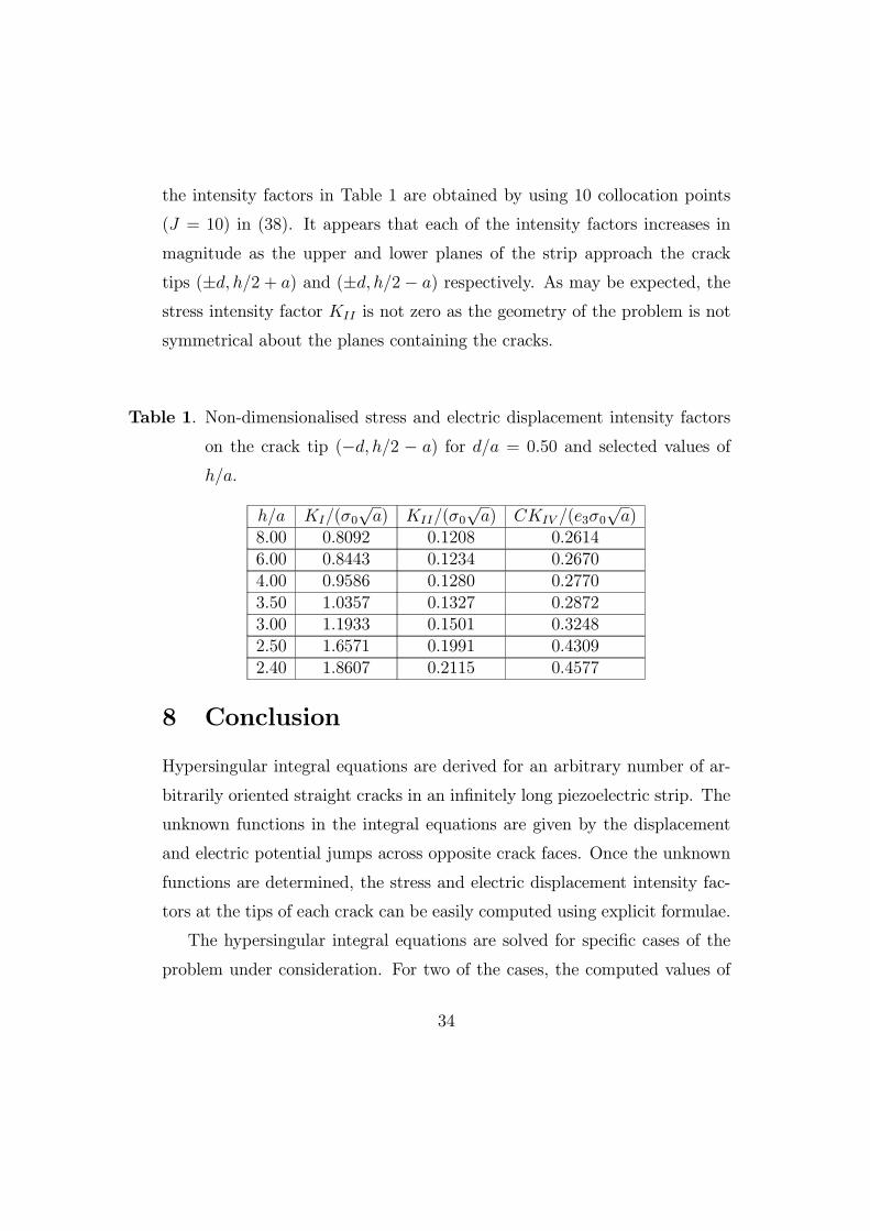
the intensity factors in Table 1 are obtained by using 10 collocation points

(J = 10) in (38). It appears that each of the intensity factors increases in

magnitude as the upper and lower planes of the strip approach the crack

tips (±d, h/2 + a) and (±d, h/2− a) respectively. As may be expected, thestress intensity factor KII is not zero as the geometry of the problem is not

symmetrical about the planes containing the cracks.

Table 1. Non-dimensionalised stress and electric displacement intensity factors

on the crack tip (−d, h/2 − a) for d/a = 0.50 and selected values of

h/a.

h/a KI/(σ0√a) KII/(σ0

√a) CKIV /(e3σ0

√a)

8.00 0.8092 0.1208 0.26146.00 0.8443 0.1234 0.26704.00 0.9586 0.1280 0.27703.50 1.0357 0.1327 0.28723.00 1.1933 0.1501 0.32482.50 1.6571 0.1991 0.43092.40 1.8607 0.2115 0.4577

8 Conclusion

Hypersingular integral equations are derived for an arbitrary number of ar-

bitrarily oriented straight cracks in an infinitely long piezoelectric strip. The

unknown functions in the integral equations are given by the displacement

and electric potential jumps across opposite crack faces. Once the unknown

functions are determined, the stress and electric displacement intensity fac-

tors at the tips of each crack can be easily computed using explicit formulae.

The hypersingular integral equations are solved for specific cases of the

problem under consideration. For two of the cases, the computed values of

34

crack tip stress and electric displacement intensity factors agree well with

those published in the literature, thus verifying the validity of the solution

presented here. The crack tip intensity factors for the other cases which have

not been previously solved exhibit qualitative features which are physically

interesting as well as intuitively acceptable.

It is possible to apply the analysis presented here to a piezoelectric strip

with edge cracks if the method for solving the relevant hypersingular integral

equations is appropriately modified as explained in Nied [11]. More generally,

the hypersingular integral equations for curved cracks can also be derived and

solved numerically as outlined in [2].

References

[1] DM Barnett and J Lothe, Dislocations and line charges in anisotropic

piezoelectric insulators, Physica Status Solidi (b) 67 (1975) 105-111.

[2] YZ Chen, A numerical solution technique of hypersingular integral equa-

tion for curved cracks, Communications in Numerical Methods in Engi-

neering 19 (2003) 645-655.

[3] DL Clements, Boundary Value Problems Governed by Second Order El-

liptic Systems, Pitman, London, 1981.

[4] F Garcia-Sanchez, A Saez and J Dominguez, Anisotropic and piezoelec-

tric materials fracture analysis by BEM, Computers & Structures 83

(2005) 804-820.

[5] AC Kaya and F Erdogan, On the solution of integral equations with

strongly singular kernels, Quarterly of Applied Mathematics 45 (1987)

105-122.

35

[6] XF Li, Electroelastic analysis of an anti-plane shear crack in a piezo-

electric ceramic strip, International Journal of Solids and Structures 39

(2002) 1097-1117.

[7] XF Li, Closed-form solution for a piezoelectric strip with two collinear

cracks normal to the strip boundaries, European Journal of Mechanics-

A/Solids 21 (2002) 981-989.

[8] XF Li and XY Duan, Closed-form solution for a mode III crack at the

mid-plane of a piezoelectric layer, Mechanics Research Communications

28 (2001) 703-710.

[9] XF Li and KY Lee, Electroelastic behavior of a rectangular piezoelectric

ceramic with an antiplane shear crack at arbitrary position, European

Journal of Mechanics-A/Solids 23 (2004) 645-658.

[10] SM Kwon and KY Lee, Analysis of stress and electric fields in a rect-

angular piezoelectric body with a center crack under anti-plane shear

loading, International Journal of Solids and Structures 37 (2000) 4859-

4869.

[11] HF Nied, Periodic array of cracks in a half-plane subjected to arbitrary

loading, ASME Journal of Applied. Mechanics 54 (1987) 642-648.

[12] E Pan, A BEM analysis of fracture mechanics in 2D anisotropic piezo-

electric solids, Engineering Analysis with Boundary Elements 23 (1999)

67-76.

[13] Y Shindo, F Narita and K Tanaka, Electroelastic intensification near

anti-plane shear crack in orthotropic piezoelectric ceramic strip, Theo-

retical and Applied Fracture Mechanics 25 (1996) 65-71.

36

[14] Y Shindo, K Watanabe and F Narita, Electroelastic analysis of a piezo-

electric ceramic strip with a central crack, International Journal of En-

gineering Science 38 (2000) 1-19.

[15] BL Wang and Mai YW, A piezoelectric material strip with a crack

perpendicular to its boundary surfaces, International Journal of Solids

and Structures 39 (2002) 4501-4524.

[16] BLWang and JC Han, Fracture of a finite piezoelectric strip with a crack

vertical to its borders-an exact analysis and applications, International

Journal of Applied Electromagnetics and Mechanics 27 (2007) 87-99.

[17] BL Wang, JC Han and SY Du, New considerations for the fracture

of piezoelectric materials under electromechanical loading, Mechanics

Research Communications 27 (2000) 435-444.

[18] BL Wang and N Noda, Mixed mode crack initiation in piezoelectric

ceramic strip, Theoretical and Applied Fracture Mechanics 34 (2000)

35-47.

[19] XC Zhong and XF Li, Closed-form solution for two collinear cracks in

a piezoelectric strip, Mechanics Research Communications 32 (2005)

401-410.

37