kalman filtersensitivit wity h respect to ... filtersensitivit wity h respect to parametric noises...

K Y B E R N E T I K A — VOLUME 32 ( 1996 ) , NUMBER 3, PAGES 3 0 7 - 3 2 2

KALMAN FILTER SENSITIVITY W I T H R E S P E C T TO P A R A M E T R I C NOISES UNCERTAINTY

N I K O L A M A D J A R O V AND LUDMILA MIHAYLOVA

The influence of the noises uncertainty on the Kalman filter performance is characterized by sensitivity functions. Relationships for computing these functions are derived and used both for synthesizing a Kalman filter with reduced sensitivity (KFRS) and a self-tuning Kalman filter (SKF). The results are illustrated by examples.

1. INTRODUCTION

The influence of the noises uncertainty on the Kalman filter behaviour is widely discussed in li terature [7, 8, 12, 13, 14, 15, 17, 20, 22, 24, 25, 26, 31]. Considerable research has been performed, for example, on the estimation of errors bounds under modeling uncertainty [24, 31], the indirect sensitivity functions that characterize the effect of each parameter variation on the error variance [5, 6], the direct sensitivity functions defined by the state vector derivative with respect to the varying parameter [13, 14], etc. The sensitivity functions can be used both as a quantitative characteristics of the filter sensitivity and in a generalized performance index for synthesizing a robust filter. The degradation of the filter performance depending on the da ta uncertainty is, obviously, closely related to the investigation of the Riccati equation sensitivity to the da ta uncertainty [1, 4, 10].

Different ideas for synthesizing a robust Kalman filter are suggested in [2, 11, 16, 21, 34]. Methods for synthesizing discrete Kalman filters, robust with respect to data outliers are proposed [2, 11]. The problem of continuous robust Kalman filter design is considered for linear systems with parameter uncertainty in both the state and measurement matrices [34]. The covariance of the filter estimation error is guaranteed to be within certain bounds for all admissible uncertainties. Strat ton and Stengel [30] develop a robust filter for predictive wind shear detection with application in aircrafts.

Another group of methods for synthesizing robust Kalman filters is related to presetting the unknown variables within the domains of their possible values. The operations over the unknown values are reduced to operations over the respective domains [23].

An alternative to the approach for synthesizing robust filters is the approach for

308 N. MADJAROV AND L. MIHAYLOVA

synthesizing adaptive filters. The estimation of the state vector in the presence of an a priori uncertainty can be done by means of different adaptive algorithms [7, 20]. The numerical characteristics of the filter innovation process are studied and minimized in most of the algorithms and "whitening" of the innovations is made. The various adaptive filtering methods for unknown noise statistics are divided into four categories [19]: Baysian, maximum likelihood, correlation and covariance matching. Indirect methods for tuning are used in a number of papers [3, 7, 20].

In the present paper the influence of the inaccurate noise covariances on the Kal-man filter performance is characterized by means of sensitivity functions. A Kalman filter with reduced sensitivity is synthesized through augmentation of the estimation error vector by the sensitivity functions. It is shown that the KFRS possesses robust properties in a wide range of variations of the noise covariances. A self-tuning Kalman filter is described using sensitivity functions and the stochastic approximation method. The filter gain is tuned directly. The obtained results are illustrated by examples.

2. PROBLEM STATEMENT

The state vector Xjt € 3£n of a linear discrete-time system

Xjfc+i = Fxk + Gvk (2.1)

is estimated on the observation of the output yk 6 3ftr

Vk = Cxk + wk, (2.2)

where the system noise vk G 3£m and the measurement noise Wk E 3£r are mutually uncorrelated white noises, with covariances Vv and Vw, respectively. Sources of parameter variations in the models (2.1), (2.2) are the noise covariances.

The inaccurate values of the covariances that are the data available for the Kalman filter synthesis will be denoted by Vv and Vw. Single-input, single-output (SISO) stationary systems are considered because the generalization for multi-input, multi-output (MIMO) and nonstationary systems constitutes no major difficulty. The normalization Vk = V^vv

k a n d Wk = y/V^Wk is used where v0. and w^ are

single covariance white noises (Vvo = Vwo = 1). The discrete-time stochastic observer is a linear filter, having the form [9]

xk+1 = Fxk + A'jfc+i (yjt+i - CF£k), (2.3)

where xk is the estimate of the state xk. The estimation error ek = Xk — Xk ls

described by the linear equation

ek+1=Aek+B[v0k,w

0k+1}T, (2.4)

where

A = (I-Kk+iC)F, B= \(I-Kk+lC)Gs/vv%-Kk+ly/vZ],

Kalman Filter Sensitivity with Respect to Parametric Noises Uncertainty 309

rp

I is the identity matrix, nk+1 = [vk,w°.+1} is a generalized white vector noise with single covariance. The variance De>k of the error ek is the Lyapunov equation solution

De,k+i = (/ - Kk+iC) Qk (I - Kk+1C)T + Kk+1VwKT+li (2.5)

where Qk = FDe>kF

T + GVvGT,

Kk+1 is the Kalman filter gain. If the gain A'jk+i is determined from the condition

dtrDeik+1 _ 0, (2.6)

dKk+1

where tr denotes the trace of the matrix, the following relationship holds

A'*+i = QkCT (CQkC

T + V _ ) _ 1 . (2.7)

When the initial noise covariances are inaccurate, i.e. Vv and Vw, the filter coefficient A'jk+i is determined from the "algorithmic" error variance Dek

Deik+1 = (I- Kk+1C) Qk (I - Kk+1C)T + Kk+1VwKTk+1, (2.8)

where _ _ Qk = FDe>kF

T + GVvGT,

Kk+1 = QkCT (CQkC

T + VW)~1. (2.9)

The algorithmic variance differs from the actual variance Deik that is the solution to the equation

De>k+1 = (/ - Kk+1C) Qk (I - Kk+1C)T + Kk+1VwKTk+l, (2.10)

Qk = FDe,kFT + GVvG

T.

The Kalman filter sensitivity with respect to variations in the covariances Vv and V_ is estimated by means of the direct sensitivity functions

.Z = f | , (2.U)

The following stochastic equations are obtained after the differentiation of (2.4) with respect to Vv and V_

4+i =Asvk + ^ = [v°k,0)T, (2.13)

B_ 2V

/V_" The variances of sk and sk are solutions to the Lyapunov equations

Dv,,k+i = U - Kk+1C) (FDlkFT + ^p) (I - Kk+iCf , (2.15)

D1Mi = (I- Kk+iC)FDlkFT(I- Kk+iCf + ^ fc+1 • (2.16)

k*+l=Ask» + -7==[Q,w0k+1}

1 . (2.14)


Example 1. The influence of the inaccurate initial information upon the Kalman filter performance is illustrated by a simple example for the steady-state mode of the filter (Dk+\ = Dk = D and A'jt+i = K). The system is described by the equations

Xk+i = xk + vk, Vv = 2,

Vk = Xk + Wk, Vw = 4.

It is obtained from (2.5) and (2.7)

- 1 De=0.Wv [yJl + AVwVv-

l-\\ = 2 ,

2 [\ + \l + WwVv-1 = 0 . 5 .

For an inaccurately known noise covariance Vw, from (2.8) and (2.9) it follows that

- l

Df 4 1 + 2 1 ^ - 1 , K = 2[ \+\\+2V

The actual error variance De is determined from (2.10) and (2.9) (for Vv and Vw)

De= (6Z 2-4A+2) [K{2-'K)}~1 , K = 2n + \JV+2~V\}j .

1 \

De

\ \

"\ X

LЪe

D e = 2 / e

y

, , -""Jч """"""^r—-—,ИÉ ,

10 V =410 w

v,„

10

Fig. 1.

The variance D™ of the sensitivity function sw is computed from (2.16)

L>" = [Ww\ \ + 2V Ф The graphics of the corresponding variances depending on Vw are shown in Figure 1. For Vw = Vw = 4 all the error variances coincide, i.e. De = De = De. Considerable


deviation of the algorithmic error variance from the actual De is observed for an inaccurate noise covariance Vw, as expected (an effect of the inner filter divergence). As Vw increases, the variance Dw of the sensitivity function sw decreases which conforms to the theory.

3. SYNTHESIS OF A KALMAN FILTER WITH REDUCED SENSITIVITY

A standard approach for synthesizing systems with reduced sensitivity is to include the sensitivity functions in the performance index. The generalized Kalman filter error is further used

e* ocsl , (3.1)

where a and 0 are weighting coefficients as it is assumed that all components of the vectors sv

k and sw are taken with some weights. The quantities referring to the synthesis of the KFRS will be denoted by an asterisk. Putting together (2.4), (2.13) and (2.14), yields that the generalized error (3.1) satisfies the equation

-k+ i — -4 ek + B 'jfc+i> (3.2)

fhere

A* = (I-Kk+1C)F 0 0

0 (I-Kk+1C)F 0 0 o (/ - Kk+1C) F

BĄ

(I-Kk+1C)Gy/VІ~

a(I-Kk+1C) G

0

2y/VZ

•Kk + 1y/Vw

0

-ß Kk+i

2vťV^

In its structure (3.2) is analogous to (2.4). Therefore the following Lyapunov equation holds

D*>k+1=A*D*€tkA*T + B*B*T (3.3)

which is analogous to (2.5) after a respective substitution of the matrices A and B with the matrices A* and B*. It is shown in Appendix 1 that the KFRS has the form

xk+1 = Fxk + K*k+1 (yk+i - CFxk), (3.4)

K*k+1 = Q*kcT (CQICT + v:yx,

Ql = FD*eikFT + GVv*GT,

„,2 p V = V, + V

v v 4VV' w Vw +

414

(3.5)

(3.6)

and the variance D*k is the solution to (2.5), i.e.

D;ik+1 = (l-K*k+1C) (FD*e>kFT + GVvG

T) (l-K*k+1C)T+ K*k+1VwK*kT

1. (3.7)


The actual variance Dk of the error ek is computed from

£>:,k+i=(l-Tk+1c) (FD:>kFT + GVvG

T) (l-Tk+1cf +Tk+1VWTT+1. (3.8)

A compromise between the filter accuracy and robustness can be achieved by an appropriate choosing of the weights a and /? (see Appendix 1).

Example 2 . The method for synthesizing a KFRS is illustrated for the system in Example 1. It is known that Vv = 2 and the accurate noise covariance Vw belongs to the interval [1,10]. The synthesis is performed for two values of Vw : Vw = 1.5 (near to Knin) and 5 (close to the middle of the interval).

Fig. 2.

When Vw = 1.5 it is computed for: - a standard Kalman filter that

= 2 (ì + ^/ì+~2vЛ - i

De =

K = 2\l + yJl + 2Vw ) =0.6667,

^ T 2 K (2 + Vw) - AK + 2 [K (2 - K)]

- ì

that

Kalman filter with reduced sensitivity 1/3 = 2VW = 3, i.e. Vw = 2VW = 3)

D: =

T = 2n + \fl + 2Vl) = 0.5486

T2 (2 + Vw) - AT + 2] [K* (2 - T)] , - 1

D\ being computed from (3.8).

When Vw = 5 (B = 2VW = 10, i.e. V*w = 2VW = lo) the expressions for De,

Dl are the same as in the case above, the new filter gains K = 0.4633, A' = 0.3583


being replaced in them. For the standard Kalman filter when the initial information is accurate

- l i - i K = 2 (1 + y/l + 2Vw) ,De= [K2 (2 + Vw) - AK + 2] [K (2 - K)]' The plots of the variances De, D*, De depending on Vw are shown in Figure 2

and Figure 3. It is seen for this example that the KFRS possesses better performance when Vw is chosen near to Vmin (Figure 2).

'" ' ! ! Í 1 I ! T • - Г —

_'__ ! ! L L l-AìLjgźi

\.Aђ^ў^\..-i-\-\-\

Í^TTІ"TT"І ' - . / . . - . . +. _ . . ¥ i Ą i i

ґ ; ; ' ! • . . . i , І i

Fig. 3.

The generalization of the KFRS synthesis for MIMO systems is performed in the same way. In this case si and s™ are matrices. The generalized error e£ comprises the sensitivity functions of every element in the matrices Vv and Vw. If the matrices are diagonal (for mutually uncorrelated system noises, resp. mutually uncorrelated measurement noises)

ejt

4 = ams ß

(3.9)

_ w where .J« = J j^ l , i = 1,2,. . . .m, sw

k> = J & t , j = 1,2,..

Appendix 1 that V* =Vv + ^ V , " 1 , V;* = V . + ^V^"1 , where

, r. It is shown in

a =

oci

0

0

ß = 0

0

/3r

and the Kalman filter equations (3.4)-(3.8) hold. The weighting matrices a and (3 can be computed according to the same conditions as in the scalar case. When any


noise covariance element is accurately known, then the respective element of a or 0 has to be set to zero.

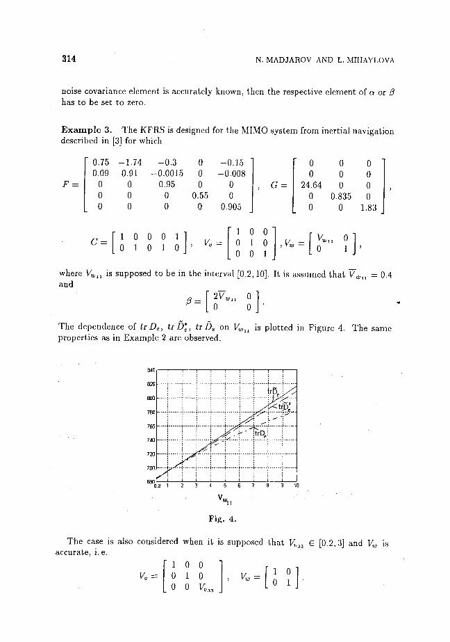
Example 3, The KFRS is designed for the MIMO system from inertial navigation described in [3] for which

F =

0.75 -1.74 0.09 0.91

0 0 0 0 0 0

-0 .3 -0.0015 0.95

0 0

0 0 0

0.55 0

-0.15 -0.008

0 0

0.905

G =

0 0 0 0 0 0

24.64 0 0 0 0.835 0 0 0 1.83

C = 1 0 0 0 1 0 1 0 1 0 , vv =

1 0 0 " 0 1 0 ,vw = 0 0 1

v W l l 0 0 1

where VWll is supposed to be in the interval [0.2,10]. It is assumed that VWll =0 .4 and

" 2VWU 0 0 0 ß

The dependence of tr De, trD*e, tr De on VWll is plotted in Figure 4. The same properties as in Example 2 are observed.

840

820

800

780

760

740

720

700

\ ïfy j/г1

1 Jű<\i —ýľž"\ : sćЛ ^r"

ЧL w" ;4í" - ~\ ' itrDe:

^^ /Ў

0.2 1 2 3 4 5 Є 7

V

Fig. 4.

The case is also considered when it is supposed that VV33 G [0.2,3] and Vw is accurate, i.e.

" 1 0 0 Vv = 0 1 0

0 0 Vv, vw =

1 0 0 1


It is assumed that VV33 = 0.3. A KFRS is synthesized for different matrices a:

a) a = 0 0 0 0 0 0 0 0 0.5

b) a = 0 0 0 0 0 0 0 0 1.5

a =

0 0 0 0 0 0 0 0 3

The plots for these a are shown in Figures 5,6,7 respectively. The KFRS in the case b) Figure 6 is more accurate than the filter in the case a) Figure 5 but for shorter interval.

Fig. 5.

Fig. 6.


Fig. 7.

4. A SELF-TUNING KALMAN FILTER

The Kalman filter gain Kk cannot be analytically computed for unknown noise covariances. It is possible to organize a procedure for direct filter gain self-tuning by the stochastic approximation method [32]

Kk = Kk-i-7k^J[vk{Kk-i)], k=l,2, (4.1)

where j k is a step,

vk = yk -CFxk-i (4.2)

is the innovation process of the filter, J [uk (A'fc_i)] = \vTVk is the performance index that has to be minimized,

w M ^ 0 ] = ^ g - the stochastic gradient. It is assumed that 7^ satisfies the conditions ensuring convergence of the recursive algorithm (4.1) [32], e.g. 7^ = I/k. It is also assumed that the system (2.1)-(2.2) is completely controllable and completely observable.

For MIMO systems the algorithm for self-tuning has the following form

xk = Fxk-i + Kkuk, (4.3)

V I Ы = -\ [{l*{vlCF))Ni>k-i + Ti>k-i (/* {FтCтvk))] , (4.4)

Kk = Kk-i-lk^J[vk{Kk-i)] (4.5)


where 7fc = f- and

Nŕ.fc-i = дK

= E™r

r(I*Vk-i)

Ћ i , f c - l —

fc-1

дKк-i = (l*"ï-i)KГr

(4.6)

(4.7)

are direct sensitivity functions, (A * H)-Kronecker product of the matrices A and B, E™r

r

a n d ^^"-permutat ion matrices [33]. It is supposed that the initial conditions £o, N£,o, T*,o are preset. The relationships (4.6) and (4.7) for computing Nx,k-i and Tf,fc-i are obtained after differentiation of the filter equation (2.3) with respect to the gain Kk-i-

The stochastic approximation convergence is slow and can be considerably improved by well selected initial conditions.

For SISO first order systems the equations (4.4)-(4.7) have the following form

Nx,k-i — Tx,k-i = Vk-i,

VJ(uk) = -CFNx,k-ivk = -CFvk-iVk-

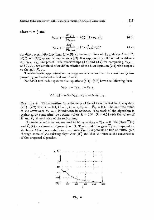
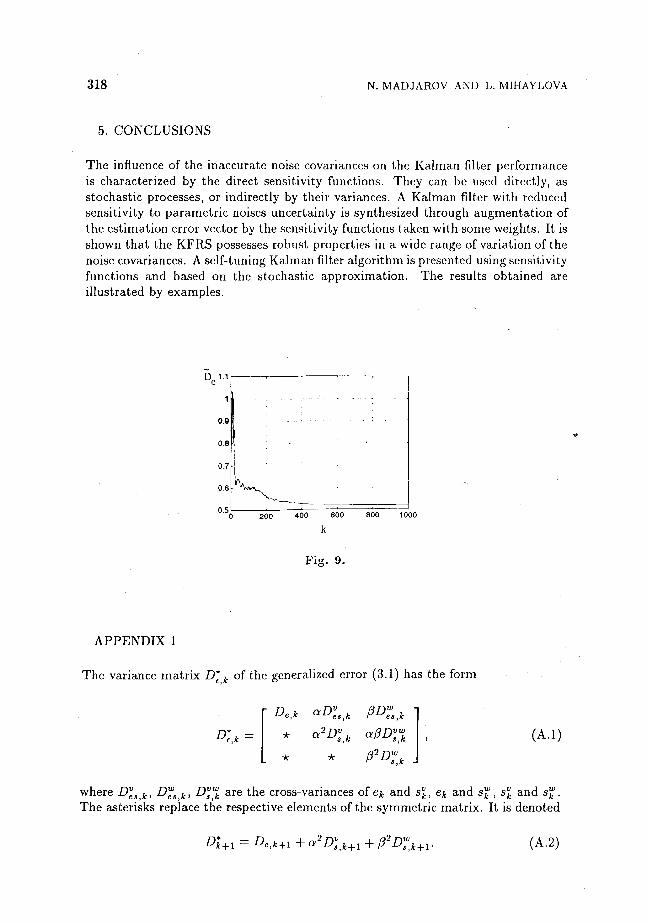
Example 4 . The algorithm for self-tuning (4.3)-(4.7) is verified for the system (2.1)-(2.2) with F = 0.4, G = 1, C = 1, Vv = l,Vw = 0.1. The accurate value of the covariance Vw = 1 is unknown in advance. The work of the algorithm is evaluated by comparing the optimal values K = 0.52, De = 0.52 with the values of K and De at each step of the self-tuning.

The initial conditions are assumed to be XQ = Nx,o = T§to = 0. The plots K(k) and De(k) are shown in Figures 8 and 9. The initial filter gain A'o is computed on the basis of the inaccurate noise covariance Vw. It is possible to find an initial gain through some of the existing algorithms [29] and thus to improve the convergence of the proposed algorithm.

1000

Fig. 8.


5. CONCLUSIONS

The influence of the inaccurate noise covariances on the Kalman filter performance is characterized by the direct sensitivity functions. They can be used directly, as stochastic processes, or indirectly by their variances. A Kalman filter with reduced sensitivity to parametric noises uncertainty is synthesized through augmentation of the estimation error vector by the sensitivity functions taken with some weights. It is shown that the KFRS possesses robust properties in a wide range of variation of the noise covariances. A self-tuning Kalman filter algorithm is presented using sensitivity functions and based on the stochastic approximation. The results obtained are illustrated by examples.

Fig. 9.

APPENDIX 1

The variance matrix D* k of the generalized error (3.1) has the form

D e.Jt

De.k aDves<k pDZ<k

«PD™k

s ,k

'e,f

* <*2D:ìk

* * p2Dls

(A.l)

where Dvs k, Dfa k, DVVJ

k are the cross-variances of ek and sk, ek and S™, sk and sk. The asterisks replace the respective elements of the symmetric matrix. It is denoted

Dî+i = D-,*+i W/ЛVн +ЃЦ?Mi. (A-2)


Taking into account (3.3), (2.5), (2.15), (2.16), (A.l) and after transformations, the following is obtained

fc-DeVl = Ér <

F0De>kFT cxFQDlskF

T ßF0DZ>kFT

* a2F0DlkFT aßF0D^kF

T

* * ß2FoDlkFT _

+

G0VVG0 + Kk+iVwKk+1 GofC70 Kfc+if Ait+i

* * A*+i4TTAT+i .

(A.З)

where FQ = (I — Kk+iC) F and C7o = (I — Kk+iC)G. On the other hand, from (A.2), (2.5), (2.15), (2.16) and after transformations, the following is derived

trD*k+1 = tr * TPT , r< I T/ , a " ^ rfT , v. ( T/ , P \ j^T FQD%Fé + G0 ( Vv + — J Gi + Kk+i \VW + ^ к + l (A.4)

Comparing (A.2), (A.3) and (A.4) yields that

trDlk+1 = trDl+1.

Hence, if the KFRS coefficient Kk+1 is determined from the condition

dtrD" e,k + l

дK 0, (A.5)

jfc+i

the relation (2.7) remains valid, if the covariances

v: = Vv + wv> K = Vw + wv:

(A-6)

are used instead of the covariances Vv and Vw. For the MIMO case (3.9), it is established in the same way that the covariances

V* and V* are formed in the following manner

Г а* 4V,.

0

; + 0 0 _

+ ...+

= vv + \ 'oc\ 0

0 " m .

0

4V„

0

= VV + TV-\(A.7)

where tt! . 0


The diagonal matrix property

VVl ••• 0 - I - 1

0 ••• VVn

is taken into account. Analogously

ß2

V* = V„ + —V~l y

w — УW I . У

W l (A.8)

where

ß = 0 ßr

The inverse matrices Vv~x and V^"1 participate in (A.7) and (A.8) which means

that only inputs and outputs with noises participate in the generalized error (3.9). The choosing of the weighting coefficients (matrices) a and /3 is a matter of a

compromise between the KFRS accuracy and robustness. From (2.4), (2.13) and (2.14) it is seen that the quantities ek, sk and sk, elements of the generalized error (3.1), are solutions to the same type equations, differing from each other by the

input variables. If the error ek and the common sensitivity sk = >k J

have to be

of equal worth in the error (3.1), the weights a and (3 have to be chosen according to the condition

B w k + 1

= в-2VV 0 + в

_ß__ 2VW w

0 o * + i J

that is satisfied if a = 2V;, ß = 2Vw (A.9)

However, the simultaneous accomplishment of conditions (A.9) results in a proportional augmentation (doubling) of the covariances Vv and Vw, because

K = Vv + ^r = 2Vv,

v: = vw + JĹ 4VW

= 2VW

This does not improve the KFRS accuracy. Really, the Riccati equation solution A,,* for Vv = K and Vw = V^and the solution D*ek when Vv* = 2STV and V^ = 2VZ are related to the condition

Dek = 2Detk,

whereas from (2.7) and (3.5) it follows that

- 1 - 1 K*+i = QtCт (CQtCт + V:) = 2QICT (2CQkCт + 2VW) = Kk+i,


i.e. the K F R S gain and the s tandard filter gain coincide. T h a t is why the condition

(A.9) has to be used only as a point of reference for the weights choosing. The same

considerations are valid for MIMO systems.

A C K N O W L E D G M E N T

The present work was supported by the Bulgarian National Fund for Scientific Research under grant TH-478/1994.

(Received October 27, 1994.)

REFERENCES

[1

[2:

[з;

[4;

[5

[6

[7

[s;

[9

[10

[11

[12

[13

[14

[15

[ie;

[17

V. Angelova, N. Christov and P. Petkov: Perturbation and numerical analysis of Kalman filters. Automatics &; Informatics (1993), 5/6, 19-20 (in Bulgarian). K. Birmiwal and J. Shen: Optimal robust filtering. Statist. Decisions 11 (1993), 101-119. B. Carew and P. Belanger: Identification of optimum filter steady-state gain for systems with unknown noise covariances. IEEE Trans. Automat. Control 18 (1973), 6, 582-587. P. Gahinet and A. Laub: Computable bounds for the sensitivity of algebraic Riccati equation. SIAM J. Control Optim. 28 (1990), 6, 1461-1480. R. E. Griffin and A. P. Sage: Large and small scale sensitivity analysis of optimum estimation algorithms. IEEE Trans. Automat. Control 13 (1968), 4, 320-329. R. E. Griffin and A. P. Sage: Sensitivity analysis of discrete filtering and smoothing algorithms. AIAA J. 7(1969), 10, 1890-1897. N.S. Gritsenko et al: Adaptive estimation: a survey. Zarubezhnaya Radioelectronica (1983), 7, 3-27 and (1985), 3, 3-26 (in Russian). A. H. Jazwinski: Stochastic Processes and Filtering Theory. Academic Press, New York 1970. R. E. Kalman: A new approach to linear filtering and prediction problems. Trans. AS ME, J. Basic Engrg. 82D (1960), 34-45. C. Kenney and G. Hewer: The sensitivity of the algebraic and differential Riccati equations. SIAM J. Control Optim. 2S (1990), 1, 50-69. B. Kovacevic, Z. Durovic and S. Glavaski: On robust Kalman filtering. Internat. J. Control 56 (1992), 3, 547-562. D. G. Lainiotis and F. L. Sims: Sensitivity analysis of discrete Kalman filters. Internat. J. Control 12 (1970), 4, 657-669. N. Madjarov and L. Mihaylova: Sensitivity analysis of linear optimal stochastic observers. In: Proc. of the IEEE Internat. Conf. on Systems, Man and Cybernetics, Systems Engineering in the Service of Humans. Le Touquet, France 1993, pp. 482-487. N. Madjarov and L. Mihaylova: Sensitivity of Kalman filters. Automatics &; Informatics (1993), 1/2, 1-18 (in Bulgarian). N. Madjarov and L. Mihaylova: Kalman filters under stochastic uncertainty. In: Proc. of the Tenth Internat. Conf. on Systems Engineering, Coventry 1994, 756-763. C. J. Masreliez and R. D. Martin: Robust Bayesian estimation for the linear model and robustifying the Kalman filter. IEEE Trans. Automat. Control 22 (1977), 3, 361-371. A. I. Matasov: The Kalman-Bucy filter accuracy in the guaranteed parameter estimation problem with uncertain statistics. IEEE Trans. Automat. Control 39 (1994), 3, 635-639.


[is:

[19

[20

[21

[22

[23

[24:

[25

[26

[27

[28

[29

[30

[31

[32

[33

[34

V. Mathews and Z. Xie: A stochastic gradient adaptive filter with gradient adaptive step size. IEEE Trans. Sign. Process. 41 (1993), 6, 2075-2087. R. K.Mehra: Approaches to adaptive filtering. IEEE Trans. Automat. Control 11 (1972), 5, 693-698. A. Moghaddamjoo: Approaches to adaptive Kalman filtering: a survey. Control Theory and Adv. Tech. 5 (1989), 1, 1-18. J.M. Morris: The Kalman filter: A robust estimator for some classes of linear quadratic problems. IEEE Trans. Inform. Theory 22 (1976), 5, 526-534. T. Nishimura: Modeling errors in Kalman filters. In: Theory and Application of Kalman Filtering (C.T. Leondes, ed.), Chapter 4, 1970, AGARDograph No. 139. M. Ogarkov: Methods for Statistical Estimation of Random Processes Parameters. Energoatomizdat, Moscow 1990 (in Russian). R. V. Patel and M. Toda: Bounds on performance of non stationary continuous-time filters under modeling uncertainty. Automatica 20 (1984), 1, 117-120. S. Sangsuk-Iam and T. Bullok: Analysis of continuous-time Kalman filtering under incorrect noise covariances. Automatica 24 (1988), 5, 659-669. S. Sangsuk-Iam and T. Bullok: Analysis of discrete-time Kalman filtering under incorrect noise covariances. IEEE Trans. Automat. Control 35 (1990), 12, 1304-1308. L. L. Scharf and D. L. Alspach: On stochastic approximation and an adaptive Kalman filter. In: Proc. of the IEEE Decision and Control Conference, 1972, pp. 253-257. N. K. Sinha: Adaptive Kalman filtering using stochastic approximation. Electr. Letters 9(1973), 819, 177-178. N. K. Sinha and A. Tom: Adaptive state estimation systems with unknown noise covariances. Internat. J. Systems Sci. 8 (1977), 4, 377-384. D.A. Stratton and R. F. Stengel: Robust Kalman filter design for predictive wind shear detection. IEEE Trans. Aerospace Electron. Systems 29 (1993), 4, 1185-1193. M. Toda and R. V. Patel: Bounds on estimation errors of discrete-time filters under modeling uncertainty. IEEE Trans. Automat. Control 26(1980), 6, 1115-1121. Ya. Z. Tsypkin: Foundations of Informational Identification Theory. Nauka, Moscow 1984 (in Russian). W. Vetter: Matrix calculus operations and Taylor expansions. SIAM Rev. 15 (1973), 2, 352-369. L. Xie and Y. Soh: Robust Kalman filtering for uncertain systems. Systems Control Lett. 22 (1994), 123-129.

Prof. Nikola Madjarov and Dipl. Eng. Ludmila Mihaylova, Faculty of Automatics, Department of Systems and Control, Technical University of Sofia, 1156 Sofia. Bulgaria.

kalman filtersensitivit wity h respect to ... filtersensitivit wity h respect to parametric noises...

Documents