Cool horizons for entangled black holes

Juan Maldacena1 and Leonard Susskind2

1 Institute for Advanced Study, Princeton, NJ 08540, USA

2 Stanford Institute for Theoretical Physics and Department of Physics,Stanford University, Stanford, CA 94305-4060, USA

Abstract

General relativity contains solutions in which two distant black holes are con-nected through the interior via a wormhole, or Einstein-Rosen bridge. These solu-tions can be interpreted as maximally entangled states of two black holes that forma complex EPR pair. We suggest that similar bridges might be present for moregeneral entangled states.

In the case of entangled black holes one can formulate versions of the AMPS(S)paradoxes and resolve them. This suggests possible resolutions of the firewall para-doxes for more general situations.

arX

iv:1

306.

0533

v2 [

hep-

th]

11

Jul 2

013

Contents

1 Introduction 2

2 Einstein Rosen Bridges 3

2.1 AdS Black Holes . . . . . . . . . . . . . . . . . . . . . . . . . . . . . . . . 3

2.2 Cool horizons for entangled black holes . . . . . . . . . . . . . . . . . . . . 6

2.3 Schwarzschild Black Holes . . . . . . . . . . . . . . . . . . . . . . . . . . . 6

2.4 Natural production of entangled black holes in the same spacetime . . . . . 8

2.5 Different bridges for different entangled states . . . . . . . . . . . . . . . . 9

2.6 Bridges for less than maximal entanglement . . . . . . . . . . . . . . . . . 12

2.7 Growth of the Bridge . . . . . . . . . . . . . . . . . . . . . . . . . . . . . . 13

3 ER= EPR 15

3.1 No Superluminal Signals . . . . . . . . . . . . . . . . . . . . . . . . . . . . 16

3.2 No Creation By LOCC . . . . . . . . . . . . . . . . . . . . . . . . . . . . . 16

3.3 Restoring the thermofield state . . . . . . . . . . . . . . . . . . . . . . . . 18

3.4 Messages From Alice to Bob . . . . . . . . . . . . . . . . . . . . . . . . . 18

3.5 Clouds . . . . . . . . . . . . . . . . . . . . . . . . . . . . . . . . . . . . . . 18

3.6 Hawking Radiation . . . . . . . . . . . . . . . . . . . . . . . . . . . . . . . 21

4 Implications for the AMPS paradox 22

4.1 Simple and Complex Operators . . . . . . . . . . . . . . . . . . . . . . . . 22

4.2 A Laboratory Example . . . . . . . . . . . . . . . . . . . . . . . . . . . . . 24

4.3 Comments on flat space AMPS . . . . . . . . . . . . . . . . . . . . . . . . 29

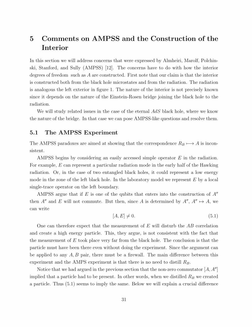
5 Comments on AMPSS and the Construction of the Interior 31

5.1 The AMPSS Experiment . . . . . . . . . . . . . . . . . . . . . . . . . . . . 31

5.2 An AMPSS like experiment for the eternal AdS black hole . . . . . . . . . 32

5.3 Information contained in A and error correction . . . . . . . . . . . . . . . 35

5.4 Linearity . . . . . . . . . . . . . . . . . . . . . . . . . . . . . . . . . . . . . 36

5.5 A Comment on phases . . . . . . . . . . . . . . . . . . . . . . . . . . . . . 37

6 Conclusion 39

A Black hole pair creation in a magnetic field 43

1

1 Introduction

Spacetime locality is one of the cornerstones in our present understanding of physics.

By locality we mean the impossibility of sending signals faster than the speed of light.

Locality appears to be challenged both by quantum mechanics and by general relativity.

Quantum mechanics gives rise to Einstein Podolsky Rosen (EPR) correlations [1], while

general relativity allows solutions to the equations of motion that connect far away regions

through relatively short “wormholes” or Einstein Rosen bridges [2]. It has long been

understood that these two effects do not give rise to real violations of locality. One

cannot use EPR correlations to send information faster than the speed of light. Similarly,

Einstein Rosen bridges do not allow us to send a signal from one asymptotic region to

the other, at least when suitable positive energy conditions are obeyed [3, 4, 5]. This is

sometimes stated as saying that Lorentzian wormholes are not traversable1.

Here we will note that these two effects are actually connected. We argue that the

Einstein Rosen bridge between two black holes is created by EPR-like correlations between

the microstates of the two black holes. This is based on previous observations in [6, 10].

We call this the ER = EPR relation. In other words, the ER bridge is a special kind of

EPR correlation in which the EPR correlated quantum systems have a weakly coupled

Einstein gravity description. It is also special because the combined state is just one

particular entangled state out of many possibilities. We note that black hole pair creation

in a magnetic field “naturally” produces a pair of black holes in this state. It is very

tempting to think that any EPR correlated system is connected by some sort of ER

bridge, although in general the bridge may be a highly quantum object that is yet to be

independently defined. Indeed, we speculate that even the simple singlet state of two spins

is connected by a (very quantum) bridge of this type.

In this article we explain the reasons for expecting such a connection. We also explore

some of the implications of this point of view for the black hole information problem, in its

AMPS(S)[11, 12] form. See [13, 14, 15] for some earlier work and [12] for a more complete

set of references. See [16] for a proposal to describe interiors that is similar to what we

are saying here2.

1This can be shown using the integrated null energy condition [4, 5], which is a correct condition inthe classical theory. It can be violated by a small amount in the quantum theory, but, as far as we know,not by enough to make wormholes traversable. We will assume that wormholes remain un-traversable inthe quantum theory. If this were not true, the ER=EPR connection would be wrong.

2For other work trying to connect two sided black holes with the AMPS paradox see [17].

2

The first point is that two black holes that are far away but connected by an ER

bridge provide an existence proof of a black hole that is maximally entangled with a

second distant system, but which nevertheless has a smooth horizon. On the other hand,

AMPS [11] suggested that the smoothness of the interior will be destroyed once the black

hole becomes entangled with another system; the second system being the radiation in

their case. If an observer collects the radiation, then, with a powerful enough quantum

computer3, she could collapse it into a second black hole which is perfectly entangled with

the first. In addition, by operations solely on her side, she can put the pair of black holes

in the special state that produces the smooth ER bridge. Thus we argue that the action

of a quantum computer on the radiation can produce a state where the horizon is smooth.

Consider the case of two very distant black holes which are entangled in the state that

produces the ER bridge. Bob is stationed at one (the near black hole) and Alice is at the

other (far black hole). Alice has a powerful quantum computer that can act on her black

hole. Then it is possible for Alice to send messages to Bob through the Einstein-Rosen

bridge. Bob cannot receive the messages as long as he is outside his horizon, but as soon

as he passes through the horizon he can receive the messages. If Alice chooses, she can

create a firewall at Bob’s end. The original AMPS experiment can be restated as sending

such a message. We see that actions on the radiation are not innocuous; they can affect

what Bob feels when he falls through the horizon.

In acting with her quantum computer on the radiation, Alice has created a very special

state. What if she does not act on the radiation at all?. A naive picture is that the

radiation would be connected by very quantum ER bridges to itself and also to the black

hole horizon. Thus, whether the black hole horizon is smooth or not depends on how these

quantum bridges connect to form the big classical geometry outside the horizon of the first

black hole. If we trust the equivalence principle, then we would conclude that the bridge

remains big and classical in the interior of the black hole. However, we do not have an

independent argument for its smoothness.

2 Einstein Rosen Bridges

2.1 AdS Black Holes

Einstein-Rosen bridges and their relation with entanglement is most rigorously understood

in the ADS/CFT framework. Consider the eternal AdS-Schwarzschild black hole whose

3We are ignoring possible limits on quantum computation [18].

3

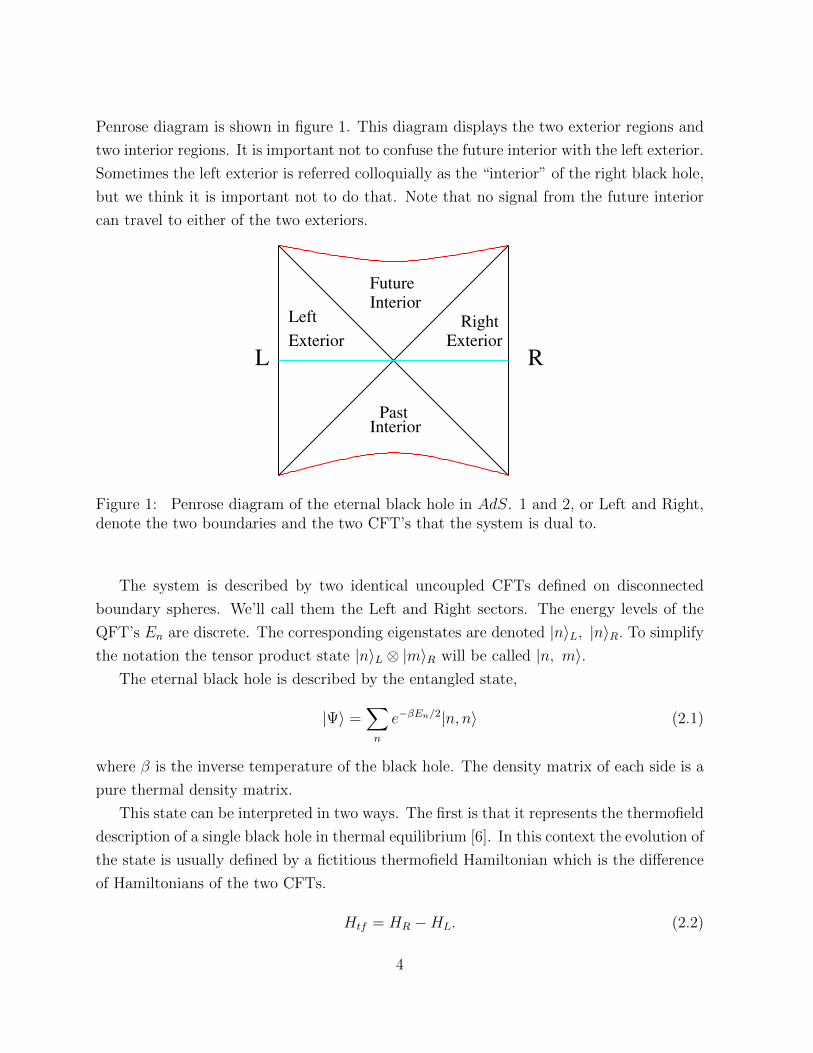
Penrose diagram is shown in figure 1. This diagram displays the two exterior regions and

two interior regions. It is important not to confuse the future interior with the left exterior.

Sometimes the left exterior is referred colloquially as the “interior” of the right black hole,

but we think it is important not to do that. Note that no signal from the future interior

can travel to either of the two exteriors.

InteriorFuture

Past Interior

L R

Left

ExteriorRight

Exterior

Figure 1: Penrose diagram of the eternal black hole in AdS. 1 and 2, or Left and Right,denote the two boundaries and the two CFT’s that the system is dual to.

The system is described by two identical uncoupled CFTs defined on disconnected

boundary spheres. We’ll call them the Left and Right sectors. The energy levels of the

QFT’s En are discrete. The corresponding eigenstates are denoted |n〉L, |n〉R. To simplify

the notation the tensor product state |n〉L ⊗ |m〉R will be called |n, m〉.The eternal black hole is described by the entangled state,

|Ψ〉 =∑n

e−βEn/2|n, n〉 (2.1)

where β is the inverse temperature of the black hole. The density matrix of each side is a

pure thermal density matrix.

This state can be interpreted in two ways. The first is that it represents the thermofield

description of a single black hole in thermal equilibrium [6]. In this context the evolution of

the state is usually defined by a fictitious thermofield Hamiltonian which is the difference

of Hamiltonians of the two CFTs.

Htf = HR −HL. (2.2)

4

The thermofield hamiltonian (2.2) generates boosts which are translations of the usual

hyperbolic angle ω. One can think of the boost as propagating upward on the right side

of the Penrose diagram, and downward on the left. The state (2.1) is an eigenvector of

Htf with eigenvalue zero, and is therefore boost invariant. The thermofield doubling of

the Hilbert space and the introduction of Htf is a trick for facilitating the calculation of

correlation functions for a system composed of a single copy. In this interpretation there

is only one asymptotic region and one black hole in a thermal state.

The second interpretation of the eternal black hole is that it represents two black holes

in disconnected spaces with a common time [7, 8, 9, 10]. We will refer to the disconnected

spaces as sheets. The degrees of freedom of the two sheets do not interact but the black

holes are highly entangled with an entanglement entropy equal to the Bekenstein Hawking

entropy of either black hole. We say that these black holes are “maximally” entangled4.

In this second interpretation the state (2.1) is represents two black holes at a particular

instant of time t = 0. In this interpretation, the time evolution is upward on both sides

with Hamiltonian

H = HR +HL. (2.3)

The state (2.1) is not an eigenvector of H. Its evolution is given by,

|Ψ(t)〉 =∑n

e−βEn/2e−2iEnt|n, n〉. (2.4)

where |n〉 is the CPT conjugate of the state |n〉.Although the state is not time-translation invariant, the individual density matrices

on either side are time-independent thermal density matrices as before. Matrix elements

of operators that depend only on one side do not depend on time. Though the total

entanglement does not depend on time, we will see that more detailed properties of this

entanglement do depend on time. The time dependence is also evident from the Penrose

diagram where one sees that the global geometry does not have an invariance under a time

isometry that shifts both asymptotic times to the future.

The entanglement has a geometric manifestation. Even though the two black holes

exist in separate non-interacting worlds, their geometry is connected by an Einstein-Rosen

bridge. The entanglement is represented by identifying the bifurcate horizons, and filling

in the space-time with interior regions behind the horizons of the black holes.

4Note that the density matrix is the thermal density matrix and not the identity matrix. By a slightabuse of language, we will still call these states “maximally entangled”.

5

2.2 Cool horizons for entangled black holes

The entangled black holes described by the Penrose diagram in figure 1 have no firewalls,

and an observer who falls through the horizon does not feel anything special. But it is

easy to change this. Let’s expand the system to include an observer Alice who lives on the

left boundary of the Penrose diagram, and can control the boundary conditions. We can

think of her as living asymptotically far away on the sheet containing the left black hole.

Alice can send message into the bulk by manipulating the boundary condition on the left

boundary.

Bob, on the other hand, lives in the bulk. He starts out on the right exterior region

and may or may not cross the horizon. It it is obvious from the Penrose diagram that

Alice cannot send a message to Bob as long as Bob does not cross the horizon of his black

hole.

If Bob does cross the horizon he can receive a message from Alice if Alice sends it early

enough (we postpone what early enough means until section 3.4). If Alice chooses, she can

send a deadly message from a point very near the lower left corner of the diagram. For

example she may shoot in a very high energy shock wave that will propagate upward to the

right very close to Bob’s horizon. This firewall has no effect on anyone outside the horizon

of Bob’s black hole, but it kills anything that passes through the horizon. Its effects also

decays exponentially as we move forwards in time along the horizon on the right.

Evidently the answer to the question—Does Bob’s black hole have a firewall?—is that

it depends on what Alice does.

One can also consider one-sided black holes in AdS. A one-sided black hole is modeled

by a single copy of AdS. In this case, we can also send a shock wave as above, by sending

in a shock wave in addition to the infalling matter. The shock wave should be timed so

that it does not escape from the black hole but lies just inside the horizon.

2.3 Schwarzschild Black Holes

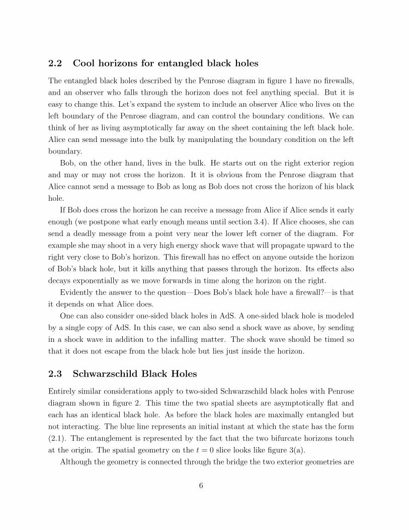
Entirely similar considerations apply to two-sided Schwarzschild black holes with Penrose

diagram shown in figure 2. This time the two spatial sheets are asymptotically flat and

each has an identical black hole. As before the black holes are maximally entangled but

not interacting. The blue line represents an initial instant at which the state has the form

(2.1). The entanglement is represented by the fact that the two bifurcate horizons touch

at the origin. The spatial geometry on the t = 0 slice looks like figure 3(a).

Although the geometry is connected through the bridge the two exterior geometries are

6

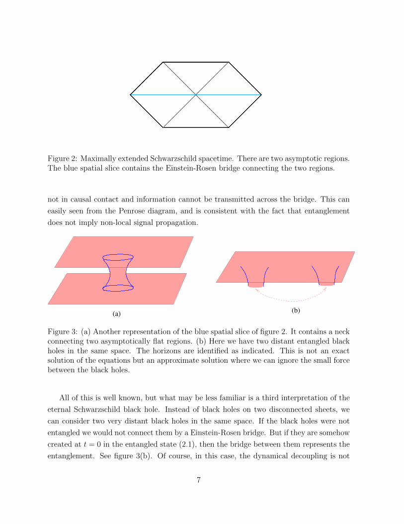
Figure 2: Maximally extended Schwarzschild spacetime. There are two asymptotic regions.The blue spatial slice contains the Einstein-Rosen bridge connecting the two regions.

not in causal contact and information cannot be transmitted across the bridge. This can

easily seen from the Penrose diagram, and is consistent with the fact that entanglement

does not imply non-local signal propagation.

(a)(b)

Figure 3: (a) Another representation of the blue spatial slice of figure 2. It contains a neckconnecting two asymptotically flat regions. (b) Here we have two distant entangled blackholes in the same space. The horizons are identified as indicated. This is not an exactsolution of the equations but an approximate solution where we can ignore the small forcebetween the black holes.

All of this is well known, but what may be less familiar is a third interpretation of the

eternal Schwarzschild black hole. Instead of black holes on two disconnected sheets, we

can consider two very distant black holes in the same space. If the black holes were not

entangled we would not connect them by a Einstein-Rosen bridge. But if they are somehow

created at t = 0 in the entangled state (2.1), then the bridge between them represents the

entanglement. See figure 3(b). Of course, in this case, the dynamical decoupling is not

7

exact, but if the black holes are far apart it is a good approximation. Note that the

black holes in 3(b) can be separated by a large distance. But an observer just outside one

horizon would be separated by a small spatial distance from an observer just outside the

other horizon, at least at t = 0.

We will imagine that Bob is stationed at one black hole which we will consider to be

the near black hole. Alice is far away at the far black hole. Near and far are of course

interchangeable but we will look at the system through Bob’s perspective. As long as Bob

and Alice stay outside their respective black hole horizons, communication between them

can only take place through the exterior space. This requires a long trip which cannot be

short-circuited by the Einstein-Rosen bridge.

On the other hand, under certain conditions Bob and Alice can jump in to their re-

spective black holes and meet very soon after.

Again in this case Alice can create a firewall on Bob’s side if she throws in shock waves

from her side early enough.

Finally we may consider one-sided black holes in flat space. These are just the ordinary

black holes created by a collapsing system in a pure state. However, we will see that

quantum theory allows one-sided black holes to eventually become two-sided, at the Page

time. At the Page time, the emitted Hawking radiation carries as many degrees of freedom

as the remaining black hole, and it is maximally entangled with the black hole. This early

half of the Hawking radiation plays the role of the second black hole and as we will see,

the question of firewalls in Bob’s black hole will be decided by what Alice, who is very far

away, decides to do with the radiation.

2.4 Natural production of entangled black holes in the samespacetime

The particular entangled state of two black holes, that we have been discussing, is very

special and one might worry that it would be extremely difficult to produce. Here we point

out that the process of black hole pair creation in an magnetic (or electric) field [19] is

such that the pair is precisely in this state.

One considers a geometry with a constant magnetic field. The pair of black holes is

described by a certain Euclidean instanton geometry, see figure 4. There is a one parameter

family of instantons that describe the creation of a pair of black holes of various sizes. The

dominant case corresponds to the creation of relatively small black holes. These black holes

are close to extremality. Extremal black holes have a fixed charge to mass ratio. This means

8

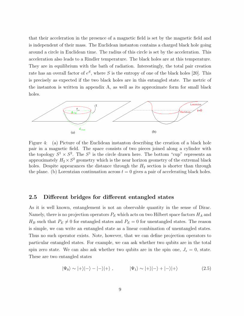
that their acceleration in the presence of a magnetic field is set by the magnetic field and

is independent of their mass. The Euclidean instanton contains a charged black hole going

around a circle in Euclidean time. The radius of this circle is set by the acceleration. This

acceleration also leads to a Rindler temperature. The black holes are at this temperature.

They are in equilibrium with the bath of radiation. Interestingly, the total pair creation

rate has an overall factor of eS, where S is the entropy of one of the black holes [20]. This

is precisely as expected if the two black holes are in this entangled state. The metric of

the instanton is written in appendix A, as well as its approximate form for small black

holes.

r

dshort

τ

d long

(a)

t=0

Lorentzian

(b)

Euclidean

Figure 4: (a) Picture of the Euclidean instanton describing the creation of a black holepair in a magnetic field. The space consists of two pieces joined along a cylinder withthe topology S1 × S2. The S1 is the circle drawn here. The bottom “cup” represents anapproximately H2×S2 geometry which is the near horizon geometry of the extremal blackholes. Despite appearances the distance through the H2 section is shorter than throughthe plane. (b) Lorentzian continuation across t = 0 gives a pair of accelerating black holes.

2.5 Different bridges for different entangled states

As it is well known, entanglement is not an observable quantity in the sense of Dirac.

Namely, there is no projection operators PE which acts on two Hilbert space factors HA and

HB such that PE 6= 0 for entangled states and PE = 0 for unentangled states. The reason

is simple, we can write an entangled state as a linear combination of unentangled states.

Thus no such operator exists. Note, however, that we can define projection operators to

particular entangled states. For example, we can ask whether two qubits are in the total

spin zero state. We can also ask whether two qubits are in the spin one, Jz = 0, state.

These are two entangled states

|Ψ0〉 ∼ |+〉|−〉 − |−〉|+〉 , |Ψ1〉 ∼ |+〉|−〉+ |−〉|+〉 (2.5)

9

There is a standard projector operator P0 = |Ψ0〉〈Ψ0| that tests whether the system is the

entangled state |Ψ0〉, and a different one that tests whether it is in the other state.

We claim that we should think of the bridges associated to these two states as being

different. In fact, we can see this clearly in the case of the eternal black hole. In this case,

we can consider the following family of Schrodinger picture states

|Ψt〉 ∼∑n

e−βEn/2e−2iEnt|n, n〉 (2.6)

Two states with different values of t are related by forward time evolution on the two sides.

However, consider them as possible alternative states at the same instant of time and view

t in (2.6) as a parameter labeling alternative states at a common instant of time. All these

states have “maximal” entanglement and the same density matrix on each side. There is a

projection operator Pt into each of these states. However, there is no projection operator

onto the whole family, since considering linear combinations such as∫dte2iE0t|Ψt〉 projects

us into a particular state |n0, n0〉, which is the one having the energy E0. This state is not

maximally entangled.

BA

(c)

BA

(b)(a)

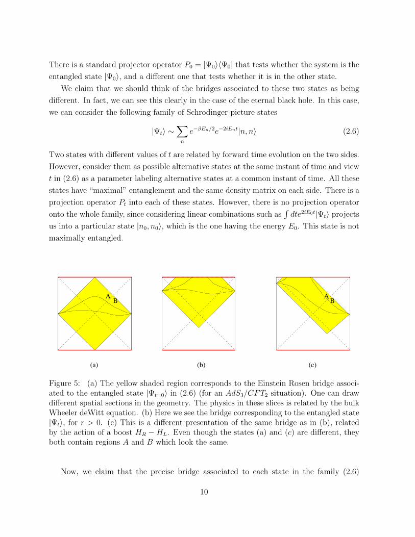
Figure 5: (a) The yellow shaded region corresponds to the Einstein Rosen bridge associ-ated to the entangled state |Ψt=0〉 in (2.6) (for an AdS3/CFT2 situation). One can drawdifferent spatial sections in the geometry. The physics in these slices is related by the bulkWheeler deWitt equation. (b) Here we see the bridge corresponding to the entangled state|Ψt〉, for r > 0. (c) This is a different presentation of the same bridge as in (b), relatedby the action of a boost HR −HL. Even though the states (a) and (c) are different, theyboth contain regions A and B which look the same.

Now, we claim that the precise bridge associated to each state in the family (2.6)

10

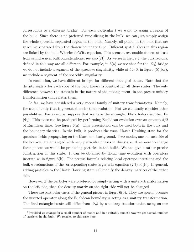
corresponds to a different bridge. For each particular t we want to assign a region of

the bulk. Since there is no preferred time slicing in the bulk, we can just simply assign

the whole spacelike separated region in the bulk. Namely, all points in the bulk that are

spacelike separated from the chosen boundary time. Different spatial slices in this region

are linked by the bulk Wheeler deWitt equation. This seems a reasonable choice, at least

from semiclassical bulk considerations, see also [21]. As we see in figure 5, the bulk regions,

defined in this way are all different. For example, in 5(a) we see that for the |Ψ0〉 bridge

we do not include a segment of the spacelike singularity, while at t > 0, in figure (5)(b,c),

we include a segment of the spacelike singularity.

In conclusion, we have different bridges for different entangled states. Note that the

density matrix for each copy of the field theory is identical for all these states. The only

difference between the states is in the nature of the entanglement, in the precise unitary

transformation that relates them.

So far, we have considered a very special family of unitary transformations. Namely,

the same family that is generated under time evolution. But we can easily consider other

possibilities. For example, suppose that we have the entangled black holes described by

|Ψ0〉. This state can be produced by performing Euclidean evolution over an amount β/2

of Euclidean time. See figure 6(a). This prescription can be used both in the bulk and

the boundary theories. In the bulk, it produces the usual Hartle Hawking state for the

quantum fields propagating on the black hole background. Two modes, one on each side of

the horizon, are entangled with very particular phases in this state. If we were to change

these phases we would be producing particles in the bulk5. We can give a rather precise

construction of this state. It can be obtained by doing time evolution with operators

inserted as in figure 6(b). The precise formula relating local operator insertions and the

bulk wavefunctions of the corresponding states is given in equation (2.7) of [10]. In general,

adding particles to the Hartle Hawking state will modify the density matrices of the either

side.

However, if the particles were produced by simply acting with a unitary transformation

on the left side, then the density matrix on the right side will not be changed.

These are particular cases of the general picture in figure 6(b). They are special because

the inserted operator along the Euclidean boundary is acting as a unitary transformation.

The final entangled state will differ from |Ψ0〉 by a unitary transformation acing on one

5Provided we change for a small number of modes and in a suitably smooth way we get a small numberof particles in the bulk. We restrict to this case here.

11

of the copies of the field theory. Depending on the precise unitary transformation we will

get states with different particles. These are further examples of different entangled states

corresponding to different bridges between the two sides.

(a) (b)

t=0 t=0

Figure 6: (a) Construction of the entangled Hartle Hawking state from Euclidean evo-lution. This creates very particular entangled bulk and boundary states. (b) We canadd particles on top of the Hartle Hawking vacuum by adding operators on the boundarytheory.

Of course, we can also consider bridges, as in figure 6(b), with an arbitrary configuration

of bulk particles. These are all different bridges corresponding to different entangled states,

though they are not all maximally entangled.

2.6 Bridges for less than maximal entanglement

In the Penrose diagrams we have discussed the Left and Right horizons touch each other.

It is also possible to have configurations where they do not touch each other. A simple

way to generate them is to start from two eternal black holes and add some matter to each

side. These configurations can also be prepared by considering Euclidean evolution with

a time dependent Hamiltonian, see [22] for some explicit solutions6. The Penrose diagram

of such configurations is given in figure 7.

6The solutions in [22] are based on Janus solutions. Their boundary in Euclidean space has the formS1×Σ where Σ is a quotient of hyperbolic space. The S1 is divided in two equal parts and the dilaton hasa different value on each part. The Lorentzian continuation is obtained by continuing across the momentwith a time reflection symmetry. The two boundaries different values for the dilaton. These values areconstant in time. The bulk smoothly interpolates between the two.

12

Right horizonLeft horizon

Minimal surface computing

the entanglement

Figure 7: Penrose diagram of a configuration obtained by analytic continuation of a timereflection symmetric, but time dependent, Euclidean solution. The two horizons do nottouch. The entanglement, computed by the Ryu-Takayanagi prescription [23], is given bythe area of a minimal surface with less area than the horizons.The area of the horizonsgrows when we go from the bifurcation point to the future.

2.7 Growth of the Bridge

Einstein-Rosen bridges are not traversable. As an observer jumps into the black hole, he

sees that the transverse two sphere shrinks as he approaches the singularity. Thus, it is

sometimes said that the bridge closes, or pinches off, before he can get through [3]. A

related feature is that as global time evolves the bridge stretches. Its length grows so fast

that no signal can get through. In figure 8 a particular slicing of the upper half of the

Figure 8: Equal time slices for the eternal black hole. The slices grow in size in theinterior. The spatial distance between opposite points on the stretched horizon grows.

13

Penrose diagram is indicated. A stretched-horizon is introduced on each side and the slices

are conventional time-slices outside the horizons. Inside they are somewhat arbitrary. An

invariant statement is that the spatial distance between a point on the L horizon and one

on the R horizon grows as we move these points to the future, keeping them on the horizon.

There seems to be an intimate connection between the entanglement of the underlying

degrees of freedom and the geometry of spacetime. A clear manifestation of this is the

Ryu-Takayanagi formula for entanglement entropy in the gauge/gravity duality [23]. Van

Raamsdonk [24] has also conjectured that the amount of entanglement between two regions

is related to their distance. The greater the entanglement the less the distance.

Time evolution is the simple innocent looking operation of adding the phases in (2.4).

We will now discuss how the entanglement grows under this operation, see [25] for further

discussion.

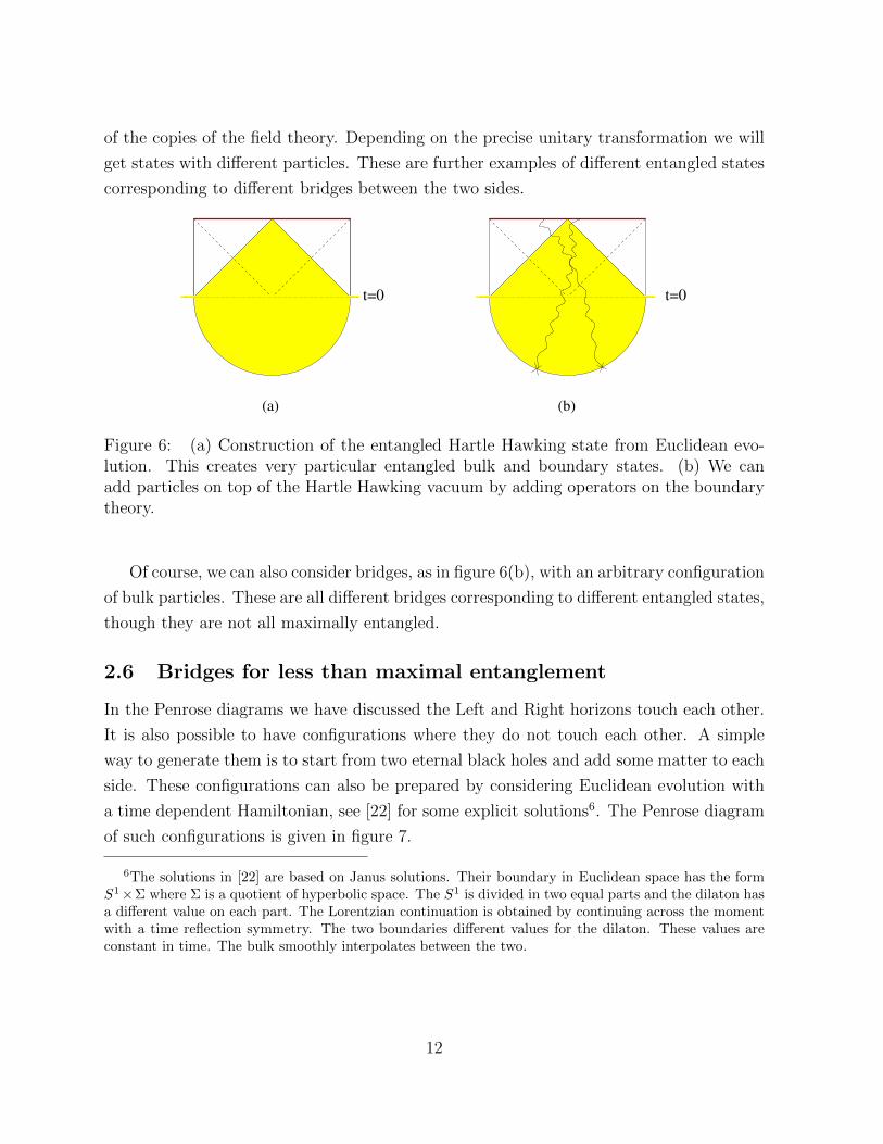
In what follows we will divide the spatial geometry in various ways. First we divide

it in the standard way into left and right halves L, R, (corresponding to CFTs L and R

shown in figure 9).

We will also make a second division into northern and southern regions, N, S, as in

figure 9. The division is not equal. The southern region is smaller than the northern.

Finally we can divide the geometry into four sectors, NL, NR, SL, SR.

We will model the degrees of freedom of these regions by a system of 2N qubits: N

for the left side and N for the right side. We can further divide them among the four

subsystems, NL, NR, SL, SR.

From the properties of the Hartle Hawking state the Left and Right qubits are initially

entangled in a state which is a tensor product of Bell pairs. The qubits are localized on

the sphere and the entanglement is between qubits at similar location. This means that

there is very little entanglement between north and south. There is however a maximal

entanglement between NL and NR and also between SL and SR.

Now we allow the system to evolve by means of the Hamiltonian H1 + H2. The time

development is a product of left and right evolution

U = U1U2 (2.7)

We expect that dynamics of each side is chaotic, and that it scrambles in a Rindler time of

order logS. After the scrambling time the operators U are represented as random matrices

in the qubit system. The effect is to scramble the entire system. We expect the following

features:

14

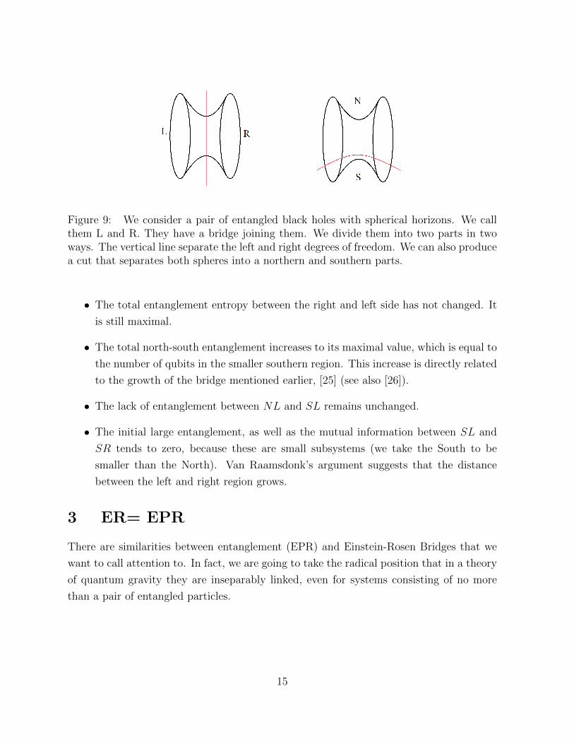
Figure 9: We consider a pair of entangled black holes with spherical horizons. We callthem L and R. They have a bridge joining them. We divide them into two parts in twoways. The vertical line separate the left and right degrees of freedom. We can also producea cut that separates both spheres into a northern and southern parts.

• The total entanglement entropy between the right and left side has not changed. It

is still maximal.

• The total north-south entanglement increases to its maximal value, which is equal to

the number of qubits in the smaller southern region. This increase is directly related

to the growth of the bridge mentioned earlier, [25] (see also [26]).

• The lack of entanglement between NL and SL remains unchanged.

• The initial large entanglement, as well as the mutual information between SL and

SR tends to zero, because these are small subsystems (we take the South to be

smaller than the North). Van Raamsdonk’s argument suggests that the distance

between the left and right region grows.

3 ER= EPR

There are similarities between entanglement (EPR) and Einstein-Rosen Bridges that we

want to call attention to. In fact, we are going to take the radical position that in a theory

of quantum gravity they are inseparably linked, even for systems consisting of no more

than a pair of entangled particles.

15

3.1 No Superluminal Signals

At first sight both entanglement and Einstein-Rosen bridges seem like strange violations

of locality, but in both cases they do not provide mechanisms for superluminal signal

propagation. It is easy to prove that no local operation on one member of a entangled pair

can influence the other, before a classical signal can propagate between them.

The situation is the same for Einstein-Rosen bridges. A look at any Penrose diagram

of a two-sided black hole easily shows that no signal can propagate through the wormhole

from one exterior region to the other.

3.2 No Creation By LOCC

In quantum information theory LOCC stands for local operations and classical commu-

nication. It refers to two separated systems—call them Alice’s and Bob’s shares— and

the possible operations that do not increase the entanglement between them. An LO op-

eration is any quantum or classical operation that Alice and Bob can do on their own

shares. This could include product unitary operations UA ⊗ UB, local measurements, or

processes involving ancillary systems. The CC of LOCC stands for classical communica-

tion. CC allows Alice to send Bob a message reporting the result of a measurement of the

z-component of spin. What she cannot do is to send the quantum spin itself. It is a basic

tenet of quantum information theory that LOCC cannot create or increase entanglement.

There are two ways to create entanglement between Alice’s and Bob’s shares. The

first is to bring them together into direct contact and allow them to interact by quantum-

mechanical interactions. The second is to have a resource of entangled qubits, which of

course had to be prepared in advance by direct interactions. If Charlie creates a collection

of Bell pairs, and sends half of each pair to Alice, and the other half to Bob, they can use

the resource to entangle their shares.

The situation for Einstein-Rosen bridges appears to be very similar. Given two distant

black holes with no Einstein-Rosen bridge, there does not seem to be any way to create

a bridge between them without preexisting bridges. However, it is possible to create a

neighboring black hole pair connected by an Einstein-Rosen bridge, and then separate the

pair.

One can also consider a pair of maximally entangled extreme black holes at zero tem-

perature. Since all the states of an extremal black hole are degenerate, the phase factors

in (2.1) are all identical. Thus the state evolves with a trivial overall phase factor that has

no physical significance. This leads to a puzzle: if the state does not evolve then it seems

16

that the Einstein-Rosen bridge does not grow with time, and it would be traversable. The

resolution is that the Einstein-Rosen bridge of an extremal black hole has infinite length

to begin with. This is just the statement that the length of the throat between the exterior

and the horizon of a charged black hole tends to infinity as the temperature tends to zero.

We point out that the area of the bridge stays finite, i.e., it does not pinch off.

The Penrose diagram describing an extremal black hole does not have two sides con-

nected by a bridge. It is not a good description of the two entangled black holes. A better

way to describe them is by using the non-extremal geometry choosing the temperature to

be below the gap to the first excited state [29].

Another way to create a bridge between two separated black holes is to use a second

pair that already has a bridge. Then by merging the members of the original pair with

the new pair, a bridge will be formed. We can even go to a suggestive extreme: create a

large number of small black-hole-pairs with bridges. Give half of each pair to Alice and

the other half to Bob and allow them to separate to a large distance. Then let Bob and

Alice each merge their own shares into a single black hole on each side. The two resulting

black holes will be connected by a bridge. In these cases the black holes might have less

than maximal entanglement, then the bridge’s neck might have an area smaller than the

area of the black hole horizon.

Finally let us make a jump. Suppose that we take a large number of particles, entangled

into separate Bell pairs, and separate them in the same way as the mini-black holes. When

we collapse each side to form two distant black holes, the two black holes will be entangled.

We make the conjecture that they will also be connected by an Einstein-Rosen bridge. In

fact we go even further and claim that even for an entangled pair of particles, in a quantum

theory of gravity there must be a Planckian bridge between them, albeit a very quantum-

mechanical bridge which probably cannot be described by classical geometry.

We summarize out conjecture with the symbolic equation,

ER = EPR (3.1)

and suggest that it is a completely general relation.

[27, 28] proposed that one needs to introduce superselection sectors in order to have

non-trivial topologies. According to the ER = EPR connection, such non-trivial topolo-

gies simply characterize the entanglement between the black holes and should be allowed

as possible quantum states.

17

3.3 Restoring the thermofield state

We can have a pair of maximally entangled black holes which are not in the thermofield

state (2.1). By assumption, the density matrix for each of the two black holes is the thermal

density matrix. We will assume that Alice has a very powerful quantum computer which

is not limited by any technological constraints. It can perform arbitrarily complicated

quantum-computations in an arbitrarily short amount of time. In this respect we are fol-

lowing the assumptions of AMPS and ignoring possible limits of computational complexity

[18]. Equipped with those powers, Alice can put her black hole into her quantum com-

puter which she has programmed to act with a unitary operator UA in the Hilbert space

of her share. This unitary operator in principle can set the state to the thermofield state

(2.1). Note that the operation does not change the entanglement entropy between Alice’s

share and Bob’s. If we had started with the thermofield state and had let it evolve so

that it acquires the phases (2.4), then Alice could “rejuvenate” it by applying the unitary

operator that reverses these phases.

3.4 Messages From Alice to Bob

Returning to the case of a near and a far black hole, we know that it is impossible for Alice

to send Bob a superluminal through the bridge, as long as Bob stays outside the horizon of

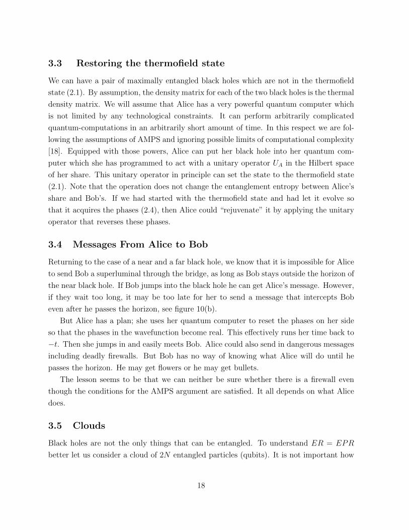
the near black hole. If Bob jumps into the black hole he can get Alice’s message. However,

if they wait too long, it may be too late for her to send a message that intercepts Bob

even after he passes the horizon, see figure 10(b).

But Alice has a plan; she uses her quantum computer to reset the phases on her side

so that the phases in the wavefunction become real. This effectively runs her time back to

−t. Then she jumps in and easily meets Bob. Alice could also send in dangerous messages

including deadly firewalls. But Bob has no way of knowing what Alice will do until he

passes the horizon. He may get flowers or he may get bullets.

The lesson seems to be that we can neither be sure whether there is a firewall even

though the conditions for the AMPS argument are satisfied. It all depends on what Alice

does.

3.5 Clouds

Black holes are not the only things that can be entangled. To understand ER = EPR

better let us consider a cloud of 2N entangled particles (qubits). It is not important how

18

L R

(a) (b)

L R

AliceBob

Alice Bobt t

Figure 10: Two black holes in the entangled thermofield state. (a) If Alice and Bob eachjump into their respective black holes, they can meet in the interior. (b) If they wait toomuch they will not meet.

they are distributed in space, but it is very important what the pattern of entanglement is.

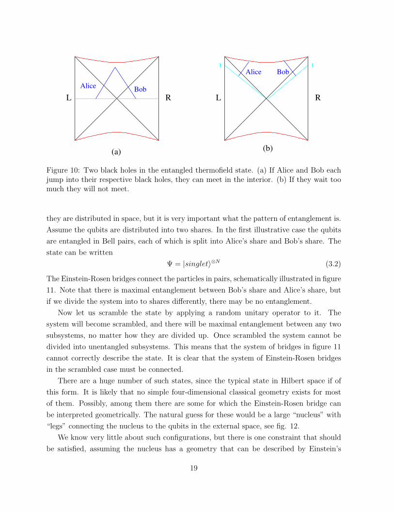
Assume the qubits are distributed into two shares. In the first illustrative case the qubits

are entangled in Bell pairs, each of which is split into Alice’s share and Bob’s share. The

state can be written

Ψ = |singlet〉⊗N (3.2)

The Einstein-Rosen bridges connect the particles in pairs, schematically illustrated in figure

11. Note that there is maximal entanglement between Bob’s share and Alice’s share, but

if we divide the system into to shares differently, there may be no entanglement.

Now let us scramble the state by applying a random unitary operator to it. The

system will become scrambled, and there will be maximal entanglement between any two

subsystems, no matter how they are divided up. Once scrambled the system cannot be

divided into unentangled subsystems. This means that the system of bridges in figure 11

cannot correctly describe the state. It is clear that the system of Einstein-Rosen bridges

in the scrambled case must be connected.

There are a huge number of such states, since the typical state in Hilbert space if of

this form. It is likely that no simple four-dimensional classical geometry exists for most

of them. Possibly, among them there are some for which the Einstein-Rosen bridge can

be interpreted geometrically. The natural guess for these would be a large “nucleus” with

“legs” connecting the nucleus to the qubits in the external space, see fig. 12.

We know very little about such configurations, but there is one constraint that should

be satisfied, assuming the nucleus has a geometry that can be described by Einstein’s

19

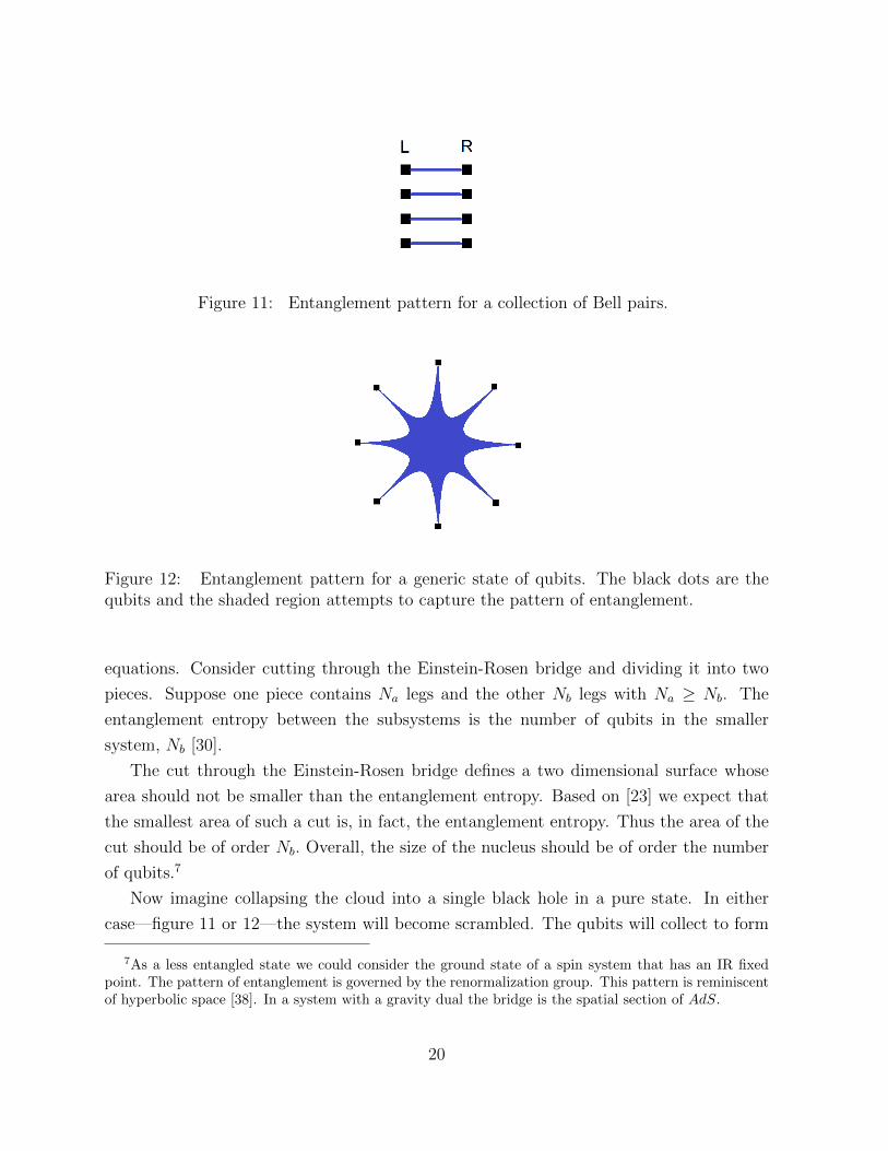
Figure 11: Entanglement pattern for a collection of Bell pairs.

Figure 12: Entanglement pattern for a generic state of qubits. The black dots are thequbits and the shaded region attempts to capture the pattern of entanglement.

equations. Consider cutting through the Einstein-Rosen bridge and dividing it into two

pieces. Suppose one piece contains Na legs and the other Nb legs with Na ≥ Nb. The

entanglement entropy between the subsystems is the number of qubits in the smaller

system, Nb [30].

The cut through the Einstein-Rosen bridge defines a two dimensional surface whose

area should not be smaller than the entanglement entropy. Based on [23] we expect that

the smallest area of such a cut is, in fact, the entanglement entropy. Thus the area of the

cut should be of order Nb. Overall, the size of the nucleus should be of order the number

of qubits.7

Now imagine collapsing the cloud into a single black hole in a pure state. In either

case—figure 11 or 12—the system will become scrambled. The qubits will collect to form

7As a less entangled state we could consider the ground state of a spin system that has an IR fixedpoint. The pattern of entanglement is governed by the renormalization group. This pattern is reminiscentof hyperbolic space [38]. In a system with a gravity dual the bridge is the spatial section of AdS.

20

the stretched-horizon and zone of the black hole. Whether or not they were initially

scrambled, after a time of order M logM they will become scrambled and therefore highly

entangled in all combinations. It seems reasonable to expect the nucleus of figure 12 will

evolve into the interior of the black hole. In other words after the scrambling time (but long

before the Page time) the interior of the black hole is the Einstein-Rosen bridge system

that connects the massively entangled near-horizon system of a black hole.

3.6 Hawking Radiation

The Hawking radiation of a black hole is a scrambled cloud of radiation entangled with

the black hole. The obvious configuration of the Einstein-Rosen bridge would resemble

the standard two-black-hole case except that Alice’s black hole would be replaced by the

Hawking radiation. We can draw a very impressionistic cartoon of the black hole connected

to the radiation by a Einstein-Rosen bridge with many exits, see figure 13.

Black holeBlack hole

.

Hawking radiationBlack hole

Figure 13: Sketch of the entanglement pattern between the black hole and the Hawkingradiation. We expect that this entanglement leads to the interior geometry of the blackhole.

Another representation is shown in figure 14. This figure shows only the geometrical

Einstein-Rosen bridge part of space. On the far left the interior of a young, one-sided black

hole is shown. The black circle represents the horizon which should be identified with the

horizon as seen from the exterior side. In the beginning there is no Hawking radiation.

As we move to the right Hawking quanta are emitted, and since they are entangled with

the black hole, they have to be connected to the bridge. The red dots represent the places

where the Hawking quanta connect to the main body of the bridge. The earlier quanta

are to the right of the later quanta. The green circles represent slices through the bridge

that divide the system into two parts. To the right of the circle the quanta were emitted

21

Figure 14: Picture of the evolution of the entanglement through a black hole’s life.

earlier than to the left. The entanglement entropy across the green circle is approximately

the number of quanta to the right. Thus as we slide the green slice to the left the area

grows. The entanglement entropy reaches a maximum at the Page time and then begins

to shrink. Thus as more quanta are emitted the horn-like figure begins to shrink. By then

the black hole has also shrunk to less than half the initial entropy.

The cartoon is speculative, and is based on the assumption that the bridge has a

geometric description. It would follow that the horizon itself is smooth and has no firewall.

Understanding the Einstein-Rosen bridge-bridge system that connects the black hole

to the radiation is the key to determining whether the horizons of evaporating black holes

are smooth. At the present time we don’t know enough to answer the question definitively.

See figure 15 for a speculation.

4 Implications for the AMPS paradox

In this section we will examine an AMPS-like paradox [11] in the context of the eternal

AdS black hole where we can use gauge-gravity duality to analyze it. We will construct a

situation in which the AMPS argument would lead to a firewall-paradox, and then debug

it.

4.1 Simple and Complex Operators

Before introducing the setup we will define some terminology. In the various discussions

of the AMPS paradox a distinction is drawn between simple and complex observables

22

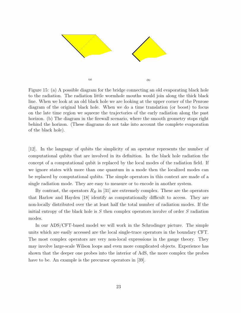
(b)(a)

Figure 15: (a) A possible diagram for the bridge connecting an old evaporating black holeto the radiation. The radiation little wormhole mouths would join along the thick blackline. When we look at an old black hole we are looking at the upper corner of the Penrosediagram of the original black hole. When we do a time translation (or boost) to focuson the late time region we squeeze the trajectories of the early radiation along the pasthorizon. (b) The diagram in the firewall scenario, where the smooth geometry stops rightbehind the horizon. (These diagrams do not take into account the complete evaporationof the black hole).

[12]. In the language of qubits the simplicity of an operator represents the number of

computational qubits that are involved in its definition. In the black hole radiation the

concept of a computational qubit is replaced by the local modes of the radiation field. If

we ignore states with more than one quantum in a mode then the localized modes can

be replaced by computational qubits. The simple operators in this context are made of a

single radiation mode. They are easy to measure or to encode in another system.

By contrast, the operators RB in [31] are extremely complex. These are the operators

that Harlow and Hayden [18] identify as computationally difficult to access. They are

non-locally distributed over the at least half the total number of radiation modes. If the

initial entropy of the black hole is S then complex operators involve of order S radiation

modes.

In our ADS/CFT-based model we will work in the Schrodinger picture. The simple

units which are easily accessed are the local single-trace operators in the boundary CFT.

The most complex operators are very non-local expressions in the gauge theory. They

may involve large-scale Wilson loops and even more complicated objects. Experience has

shown that the deeper one probes into the interior of AdS, the more complex the probes

have to be. An example is the precursor operators in [39].

23

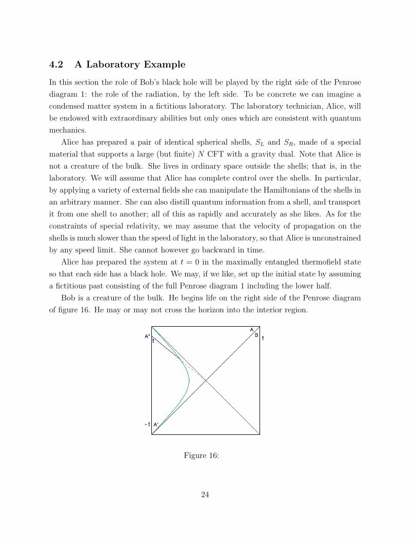
4.2 A Laboratory Example

In this section the role of Bob’s black hole will be played by the right side of the Penrose

diagram 1: the role of the radiation, by the left side. To be concrete we can imagine a

condensed matter system in a fictitious laboratory. The laboratory technician, Alice, will

be endowed with extraordinary abilities but only ones which are consistent with quantum

mechanics.

Alice has prepared a pair of identical spherical shells, SL and SR, made of a special

material that supports a large (but finite) N CFT with a gravity dual. Note that Alice is

not a creature of the bulk. She lives in ordinary space outside the shells; that is, in the

laboratory. We will assume that Alice has complete control over the shells. In particular,

by applying a variety of external fields she can manipulate the Hamiltonians of the shells in

an arbitrary manner. She can also distill quantum information from a shell, and transport

it from one shell to another; all of this as rapidly and accurately as she likes. As for the

constraints of special relativity, we may assume that the velocity of propagation on the

shells is much slower than the speed of light in the laboratory, so that Alice is unconstrained

by any speed limit. She cannot however go backward in time.

Alice has prepared the system at t = 0 in the maximally entangled thermofield state

so that each side has a black hole. We may, if we like, set up the initial state by assuming

a fictitious past consisting of the full Penrose diagram 1 including the lower half.

Bob is a creature of the bulk. He begins life on the right side of the Penrose diagram

of figure 16. He may or may not cross the horizon into the interior region.

Figure 16:

24

Following AMPS we also consider a pair of modes, A and B, situated on either side

of the horizon of Bob’s black hole. Both modes correspond to waves propagating toward

the upper right, see fig. 16. We can define the time of the A,B pair as the time where B

arrives at the right boundary.

The A,B modes can be considered to be two entangled qubits. They correspond to

modes with a wavelength larger than the Planck scale and an energy comparable to the

temperature, so that their entanglement is close to maximal. Following AMPS [11] we

may follow B out to the boundary (asymptotic infinity in the AMPS case) and identify B

as a simple operator in the right-side CFT.

In the thermofield state, B is maximally entangled with a mode on the left side of the

Penrose diagram, at a point obtained by rotating the diagram by 180-degrees about the

origin. That brings us to the operator A′ at time −t. Evidently B is entangled with both

A and A′, but there is no contradiction since A and A′ are not independent. In fact the

Penrose diagram suggests that we obtain A from bulk evolution from A′. Note that this

evolution could depend on signals that come from the right side. Namely, an object falling

from the right could flip the qubit, for example. We then write

A′ 7−→ A (4.1)

indicating that A′ determines A through bulk evolution.

One may question the use of low energy bulk equations, particularly when t is very

late. Replacing A′ by an operator on the initial condition surface t = 0 would involve

exponentially small wavelengths. We will come back to this point. For the moment we can

Lorentz boost the diagram so that B and A′ are transformed to t = 0. In this configuration

no large energies are encountered in propagating from A to A′.

Keeping in mind that A is a qubit, and therefore has three components (the Pauli

operators) we write the commutation relations

[Ai, Aj] = iεijkAk 6= 0 (4.2)

Using (4.1) allows us to write

[A′i, Aj] 6= 0. (4.3)

Let us return to the question of replacing A′ by an operator on the initial condition

surface t = 0. In quantum field theory this procedure would involve solving the equations of

motion and expressing A′ in terms of operators defined on the t = 0 surface. By inspection

we can see that only operators in the left wedge would be involved. But it is obvious that

25

for large t the result would be a trans-plankian operator of exponentially small wavelength.

The bulk procedure would be completely out of control if t is greater than the scrambling

time. However, here is where the power of gauge/gravity duality comes into play. The

operator A′ is a simple local boundary operator in the Hilbert space of the left CFT. In

principle the gauge-theory equations of motion allow us to solve for it in terms of operators

at t = 0.

Of course the chaotic nature of the dynamics will insure that A′ evolves to a very

complex operator if t is greater than the scrambling time, but the evolution is nonetheless

well defined.

The gauge-theory equations of motion are far too difficult to actually solve, but the

solution must exist. One does not expect it to involve exponentially small wavelengths, but

rather a complex gauge-theory operator. Evidently acting with A′ at time −t is equivalent

to acting with an extremely scrambled non-local operator at time 0. One point to keep in

mind is that the evolution of A′ does not involve operators in the right CFT.

We can go further and run A′ all the ways up to time t from time −t to time +t using

the equations of motion and Hamiltonian of the left shell. The two shells do not interact

so running A′ forward produces an operator A′′ at time t which also lives entirely in the

Hilbert space of the left CFT. A′′ is defined by

A′′ = e−2iHLtA′e2iHLt = ULA′U †L (4.4)

These are Schrodinger picture operators. A′′ is the operator at time t that has exactly the

same information as A′ at time −t. Thus we may write

A′′ 7−→ A . (4.5)

A′′ is a low energy operator of the same energy as B. It is far from being a local bulk

field, but it acts on the black hole as an operator with energy comparable to the Hawking

temperature. It is natural to identify it as a degree of freedom in the stretched horizon of

the left black hole. This is quite contrary to the naive expectation that the interior of the

right black hole should be built from degrees of freedom in its own stretched horizon. We

have defined A′′ as an operator in the boundary theory. We have defined A as an operator

in the bulk, which is the bulk evolution of the operator A′. The operator A′ can be viewed

as a bulk or boundary operator, with the translation being simple in this case. The arrow

in (4.5) involves bulk evolution. It depends on the structure of the bridge or the entangled

state. In other words, if we send a wave from the right that flips the spin in the evolution

26

from A′ to A, then in order to be talking about the same A, we need to modify A′ and

thus also A′′.

Another important observation is that A′′ does not commute with A. We can replace

(4.2) schematically by8

[A′′i , Aj] = iεijkAk. (4.6)

The operator A′′ plays the same role as RB in [31]. Namely, it is an operator in the

radiation subsystem (here the left CFT) that is maximally entangled with the qubit B of

the right-side black hole. Contrary to what is assumed in AMPSS, (4.6) indicates that RB

does not commute with A. The disturbance in A when Alice measures or distills A′′ will

play a central role in understanding the AMPS paradox. In AMPS there were two distant

systems, the black hole and the radiation that was entangled with it. The qubit RB ( here

A′′) was distilled by doing a computation on the radiation, and then given to Bob. Here

we can do the same. We can distill A′′, the lab technician can then take it from one shell

to the other and give it to Bob as some excitation introduced from the UV boundary of

his region.

We now have all the ingredients to construct an AMPS-like argument. At time t

The mode B is entangled with a system, A′′, which may be regarded as distant. By the

monogamy of entanglement B cannot be entangled with A. Therefore there is a firewall.

The fallacy is clear in this case; namely A′′ and A are not independent degrees of

freedom even though they are very distant in the external space. Indeed, by construction

A′′ determines A. A depends on information from both sides, from both conformal field

theories. This is the analog of the what in [31] was called A = RB. Here RB = A′′. Thus

more precisely what have is RB 7−→ A, where the mapping also depends on information

from the black hole microstates, since an object that falls into the black hole can flip the

A state.

Let’s follow the AMPS line of reasoning further: first a simplified version, see figure

17. Alice extracts the qubit A′ at time −t from the left shell and carries it across to the

right shell. She then transfers it into the right shell and gives it to Bob. She does this just

in time so that Bob can jump into the black hole and test the AB entanglement. We may

imagine that Bob carries A′. Does Bob discover that the A,B system has been corrupted?

He does, but the reason is not a firewall. The reason is that A′ does not commute with A.

When Alice extracted A′ she produces a particle in the mode A. That particle is detected

8We say “schematically” because A′′ is a boundary operator and A is bulk operator. Here we want toemphasize that we cannot distill one without modifying the other.

27

by Bob. But the corruption is restricted to a single A,B pair, and does not affect other

modes. In any case the corruption was created by Alice when she extracted A′. This case

is simpler because there is no complicated distillation process to be done, the extraction

of A′ is fairly straightforward.

It is worth noting that Bob would detect the particle even if he had no knowledge that

Alice had distilled A′.

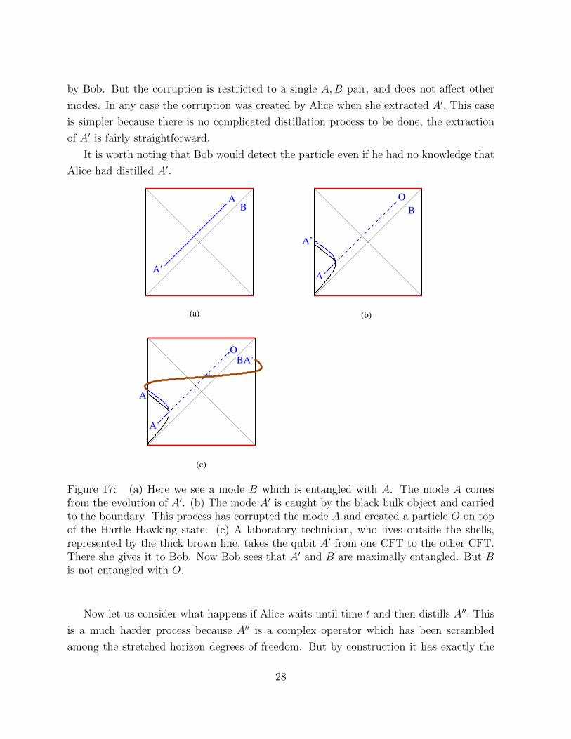
(a)

(c)

(b)

AB

A’

B

O

A’

A’

A

O

A’

BA’

Figure 17: (a) Here we see a mode B which is entangled with A. The mode A comesfrom the evolution of A′. (b) The mode A′ is caught by the black bulk object and carriedto the boundary. This process has corrupted the mode A and created a particle O on topof the Hartle Hawking state. (c) A laboratory technician, who lives outside the shells,represented by the thick brown line, takes the qubit A′ from one CFT to the other CFT.There she gives it to Bob. Now Bob sees that A′ and B are maximally entangled. But Bis not entangled with O.

Now let us consider what happens if Alice waits until time t and then distills A′′. This

is a much harder process because A′′ is a complex operator which has been scrambled

among the stretched horizon degrees of freedom. But by construction it has exactly the

28

same effect as extracting A′. In particular, because of (4.6) it creates a particle in mode

A. As before, Bob sees that B is entangled with A′ but not with O.

The important point is that the quantum detected by Bob was created by Alice when

she distilled A′′. Contrary to the AMPS assumption, it would not have been there if Alice

had not created it in the process.

Note that this example shows that the problem in AMPS is real. Extracting the qubit

entangled with B from the system that the R black hole was entangled with (which is the

L black hole) has made it impossible to preserve its entanglement with A.

This example demonstrates that entanglement of Bob’s black hole with a second system

does not imply the existence of a firewall.

4.3 Comments on flat space AMPS

Let us now return to black holes in flat space. Consider a black hole that has evaporated

past the Page time. Alice has been gathering the Hawking radiation and has more than

half of it under her control. Bob has no idea that Alice is out there with her quantum

computer. In this version of the argument, Alice takes the radiation and puts it into her

quantum computer where she converts it to a black hole. Let’s assume for simplicity that

the radiation has left Bob’s black hole with no off diagonal elements in its density matrix.

The far black hole (Alice’s) and the near black hole (Bob’s) are entangled. Alice can

operate on her black hole and create the thermofield state (2.1). When Bob jumps in he

finds a smooth horizon.

Following AMPS we consider a mode of the Bob’s zone which is about to be radiated.

The mode is called B. At an earlier time, Alice has distilled a qubit from her black hole;

namely the qubit that B will be entangled with. In distilling it she has separated it from

her black hole and turned it into an ordinary localized qubit. Following the notation in

[31] we call that qubit RB. With RB in her possession, Alice flies back to the black hole

in time to meet B as it is emitted. As AMPS argued, since B and RB are entangled, it

is not possible for B to be entangled with the mode A (behind the horizon) that it would

normally be entangled with. This disruption of the A,B entanglement means that Alice

will encounter an unexpected particle as she crosses the horizon.

AMPS then goes on to say that it did not matter that Alice carried out the experiment.

Even if she had not done so, that high energy quantum would have been there. By that

logic, every possible AB pair is corrupted and the black hole horizon becomes a firewall.

We argue AMPS only proved this:

29

If Alice does the experiment of a given B-mode, she will discover that the corresponding

AB entanglement has been corrupted for that one pair.

The argument does not prove that any other AB pair is corrupted. To go further,

AMPS must make the assumption that even if Alice did not do the experiment the AB

entanglement would be corrupted.

But in our view the particle was created at the other end of the Einstein-Rosen bridge

when Alice distilledRB. There is no reason why more than oneAB pair should be corrupted

by this process. In the eternal black hole example, we saw this very clearly.

Now Bob will be surprised that he encounters a particle as he goes into the black hole.

How did this particle get there? The answer is through the Einstein-Rosen bridge that

joins the radiation with the black hole interior. These seem very distant in the external

space, but they can be close via the Einstein-Rosen bridge bridge.

In this example, we have imagined that Alice has processed the radiation to produce

the thermofield state. Alice can do various things with her quantum computer. She can

arrange to throw a bomb at Bob. Alice can arrange to get the bomb to Bob in time to

intercept Bob as long as Bob in on the inside. In that case Bob will meet a kind of firewall.

Of course what Alice does is predetermined (in the sense of quantum mechanics) by

the initial state of the entire system. But even so, all that can be said, given the exact

initial state, is that there is a probability that Bob sees a smooth featureless horizon, and

a probability that he gets hit by a firewall, or anything else.

A good question that we can ask is: what is the probability for Bob to see any particular

thing just behind the horizon, given that a black hole forms from a definite initial state

and Alice does not interfere with the radiation? The collapse of a gas cloud in some

pure initial state in otherwise empty space would be a good example. Is the probability

distribution dominated by firewalls or by smooth featureless empty space? At the moment

both seem consistent. The answer depends on the nature of the Einstein-Rosen bridge

bridge that connects the black hole system with the Hawking radiation. If it has a smooth

geometry, similar to the standard Einstein-Rosen bridge near the horizon, then firewalls

will be improbable. If it is highly singular then smooth horizons will be improbable. We

do not know enough to answer this question. Of course, effective field theory around a

black hole horizon suggests that the horizon will be smooth. Hopefully, we have given

enough reasons for not believing the AMPS argument that there had to be firewalls.

30

5 Comments on AMPSS and the Construction of the

Interior

In this section we will address concerns that were expressed by Almheiri, Marolf, Polchin-

ski, Stanford, and Sully (AMPSS) [12]. The concerns have to do with how the interior

degrees of freedom such as A are constructed. First note that our claim is that the interior

is constructed both from the black hole microstates and from the radiation. The radiation

is analogous the left exterior in figure 1. The nature of the interior is not precisely known

since it depends on the nature of the Einstein-Rosen bridge joining the black hole to the

radiation.

We will study related issues in the case of the eternal AdS black hole, where we know

the nature of the bridge. In that case we can pose AMPSS-like questions and resolve them.

5.1 The AMPSS Experiment

The AMPSS paradoxes are aimed at showing that the correspondence RB 7−→ A is incon-

sistent.

AMPSS begins by considering an easily accessed simple operator E in the radiation.

For example, E can represent a particular radiation mode in the early half of the Hawking

radiation. Or, in the case of two entangled black holes, it could represent a low energy

mode in the zone of the left black hole. In the laboratory model we represent E by a local

single-trace operator on the left boundary.

AMPSS argue that if E is one of the qubits that enters into the construction of A′′

then A′′ and E will not commute. But then, since A is determined by A′′, A′′ 7→ A, we

can write

[A,E] 6= 0. (5.1)

One can therefore expect that the measurement of E will disturb the AB correlation

and create a high energy particle. This, they argue, is not consistent with the fact that

the measurement of E took place very far from the black hole. The conclusion is that the

particle must have been there even without doing the experiment. Since the argument can

be applied to any A,B pair, there must be a firewall. The main difference between this

experiment and the AMPS experiment is that there is no need to distill RB.

Notice that we had argued in the previous section that the non-zero commutator [A,A′′]

implied that a particle had to be present. In other words, when we distilled RB we created

a particle. Thus (5.1) seems to imply the same. Below we will explain a crucial difference

31

between measuring E and measuring A′′.

5.2 An AMPSS like experiment for the eternal AdS black hole

Here we consider the same set up as in section 4.2. The easy mode E will be a low energy

gravity mode in the bulk, or a single trace operator smeared over a region of order the

temperature of the black hole. According to the bulk geometry, when we measure E at

late times on the left, we create a disturbance in the bulk that moves forwards to the

singularity but does not affect A, see figure 18. E is spacelike separated from A and for

this reason they commute, at least as far as the bulk is concerned.

From the point of view of the boundary theory we appear to get a different picture.

The operator A′′ which is the time evolution of A′ is quite scrambled, so expect that [E,A′′]

is non-zero. This seems to contradict the bulk picture.

Why do we get two different results? We think that the addition of E changes how

we realize A in the boundary theory in terms of the boundary Hilbert space. However,

this change is such that it does not affect the local physics around A. In other words, the

physics around A is described in terms of a local Hilbert space HA. This Hilbert space

describes the presence or absence of various modes in the neighborhood of the bulk region

where A is located. This Hilbert space is embedded in the boundary Hilbert space in a way

that depends on the bridge, on the shape of the spacetime connecting it to the boundary.

As we act with E we are changing the shape of this bridge and the way in which HA is

embedded. However, this change is such that we can still extract the underlying state in

HA that we had in the bulk. In the next subsections we hope to explain this in more detail

by giving simple examples.

Note that this issue is similar to the problem of bulk locality in AdS/CFT. We can

imagine a glueball deep inside AdS as analogous to A. We can then consider an operator E

which is given by a local operator in the boundary theory, say T (x). Since A has a rather

complex expression in terms of the local degrees of freedom, we might naively expect

that [A, T (x)] 6= 0. In fact, if T is the stress tensor this commutator is indeed non-zero.

However, the bulk description suggests that this commutator should be effectively zero. In

this particular case, the answer is simple. The operator A, which creates a glueball in the

center of AdS is not gauge invariant. If we were dealing with an ordinary gauge theory

in the interior, then A would be a charged particle, and this charge can be measured at

infinity. Thus, A does not commute with the current j at infinity. The gauge invariant

version of A contains a Wilson line that goes to infinity and is non-local. This is the reason

32

B

A

A’

A’’

E

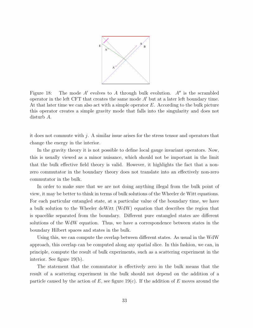
Figure 18: The mode A′ evolves to A through bulk evolution. A′′ is the scrambledoperator in the left CFT that creates the same mode A′ but at a later left boundary time.At that later time we can also act with a simple operator E. According to the bulk picturethis operator creates a simple gravity mode that falls into the singularity and does notdisturb A.

it does not commute with j. A similar issue arises for the stress tensor and operators that

change the energy in the interior.

In the gravity theory it is not possible to define local gauge invariant operators. Now,

this is usually viewed as a minor nuisance, which should not be important in the limit

that the bulk effective field theory is valid. However, it highlights the fact that a non-

zero commutator in the boundary theory does not translate into an effectively non-zero

commutator in the bulk.

In order to make sure that we are not doing anything illegal from the bulk point of

view, it may be better to think in terms of bulk solutions of the Wheeler de Witt equations.

For each particular entangled state, at a particular value of the boundary time, we have

a bulk solution to the Wheeler deWitt (WdW) equation that describes the region that

is spacelike separated from the boundary. Different pure entangled states are different

solutions of the WdW equation. Thus, we have a correspondence between states in the

boundary Hilbert spaces and states in the bulk.

Using this, we can compute the overlap between different states. As usual in the WdW

approach, this overlap can be computed along any spatial slice. In this fashion, we can, in

principle, compute the result of bulk experiments, such as a scattering experiment in the

interior. See figure 19(b).

The statement that the commutator is effectively zero in the bulk means that the

result of a scattering experiment in the bulk should not depend on the addition of a

particle caused by the action of E, see figure 19(c). If the addition of E moves around the

33

part of the Hilbert space responsible for the region A, then this dependence cancels out

when we overlap the initial and final states taking this dependence into account.

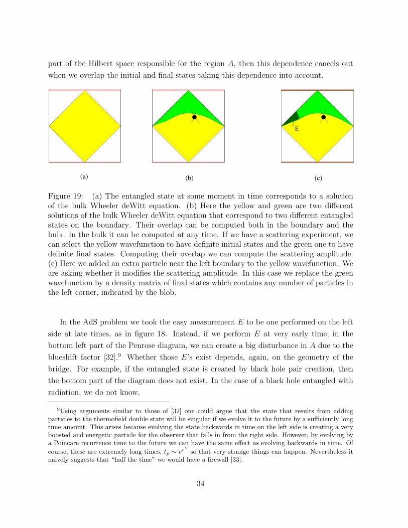
(b)(a) (c)

E

Figure 19: (a) The entangled state at some moment in time corresponds to a solutionof the bulk Wheeler deWitt equation. (b) Here the yellow and green are two differentsolutions of the bulk Wheeler deWitt equation that correspond to two different entangledstates on the boundary. Their overlap can be computed both in the boundary and thebulk. In the bulk it can be computed at any time. If we have a scattering experiment, wecan select the yellow wavefunction to have definite initial states and the green one to havedefinite final states. Computing their overlap we can compute the scattering amplitude.(c) Here we added an extra particle near the left boundary to the yellow wavefunction. Weare asking whether it modifies the scattering amplitude. In this case we replace the greenwavefunction by a density matrix of final states which contains any number of particles inthe left corner, indicated by the blob.

In the AdS problem we took the easy measurement E to be one performed on the left

side at late times, as in figure 18. Instead, if we perform E at very early time, in the

bottom left part of the Penrose diagram, we can create a big disturbance in A due to the

blueshift factor [32].9 Whether those E’s exist depends, again, on the geometry of the

bridge. For example, if the entangled state is created by black hole pair creation, then

the bottom part of the diagram does not exist. In the case of a black hole entangled with

radiation, we do not know.

9Using arguments similar to those of [32] one could argue that the state that results from addingparticles to the thermofield double state will be singular if we evolve it to the future by a sufficiently longtime amount. This arises because evolving the state backwards in time on the left side is creating a veryboosted and energetic particle for the observer that falls in from the right side. However, by evolving bya Poincare recurrence time to the future we can have the same effect as evolving backwards in time. Of

course, these are extremely long times, tp ∼ eeS

so that very strange things can happen. Nevertheless itnaively suggests that “half the time” we would have a firewall [33].

34

5.3 Information contained in A and error correction

Here we would like to emphasize that the action of the simple operator E does not destroy

the information that is highly delocalized. As a simple argument consider the following.

Note that B is almost maximally entangled with any subsystem that contains more than

half the total number of degrees of freedom. For example, in figure 20 we show a system

of 70 qubits with the qubit at the upper left corner representing B. Two subsystems, each

Figure 20:

with more than half the total number of qubits, are shown in blue. Moreover the overlap

between the two subsystems can be small. In either of these subsystems we can find a

qubit that is maximally entangled with B, which we are calling RB. In this way different

candidates for RB can be constructed.

Now assume that E was contained in the construction of RB. One can always choose

another R′B that does not involve E. R′B is also almost maximally entangled with B and

contains the same quantum information as RB to a very high approximation. But

[R′B, E] = 0. (5.2)

Thus if we identify R′B with A, the measurement of E does not disturb the AB system.

We suggest that the correct prescription is to always employ an R′B that commutes

with E.

As another argument that the information contained in A is not destroyed by the easy

measurement E, we can make an analogy with quantum error correction. The connection

with error correction was also studied in [35]. We view A as a message that has been

encoded in the radiation. The action of the operator E can be viewed as an error. These

errors act in a simple way in the radiation basis, which we view as the computational

basis. Because the radiation system is in a random state one expects the encoding of A

35

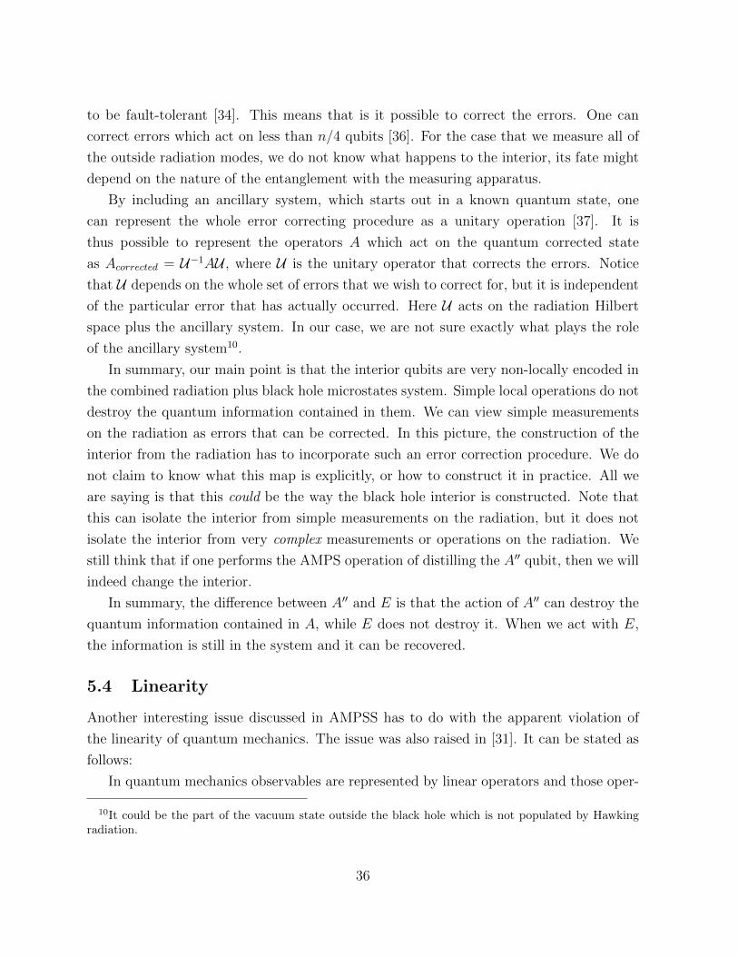
to be fault-tolerant [34]. This means that is it possible to correct the errors. One can

correct errors which act on less than n/4 qubits [36]. For the case that we measure all of

the outside radiation modes, we do not know what happens to the interior, its fate might

depend on the nature of the entanglement with the measuring apparatus.

By including an ancillary system, which starts out in a known quantum state, one

can represent the whole error correcting procedure as a unitary operation [37]. It is

thus possible to represent the operators A which act on the quantum corrected state

as Acorrected = U−1AU , where U is the unitary operator that corrects the errors. Notice

that U depends on the whole set of errors that we wish to correct for, but it is independent

of the particular error that has actually occurred. Here U acts on the radiation Hilbert

space plus the ancillary system. In our case, we are not sure exactly what plays the role

of the ancillary system10.

In summary, our main point is that the interior qubits are very non-locally encoded in

the combined radiation plus black hole microstates system. Simple local operations do not

destroy the quantum information contained in them. We can view simple measurements

on the radiation as errors that can be corrected. In this picture, the construction of the

interior from the radiation has to incorporate such an error correction procedure. We do

not claim to know what this map is explicitly, or how to construct it in practice. All we

are saying is that this could be the way the black hole interior is constructed. Note that

this can isolate the interior from simple measurements on the radiation, but it does not

isolate the interior from very complex measurements or operations on the radiation. We

still think that if one performs the AMPS operation of distilling the A′′ qubit, then we will

indeed change the interior.

In summary, the difference between A′′ and E is that the action of A′′ can destroy the

quantum information contained in A, while E does not destroy it. When we act with E,

the information is still in the system and it can be recovered.

5.4 Linearity

Another interesting issue discussed in AMPSS has to do with the apparent violation of

the linearity of quantum mechanics. The issue was also raised in [31]. It can be stated as

follows:

In quantum mechanics observables are represented by linear operators and those oper-

10It could be the part of the vacuum state outside the black hole which is not populated by Hawkingradiation.

36

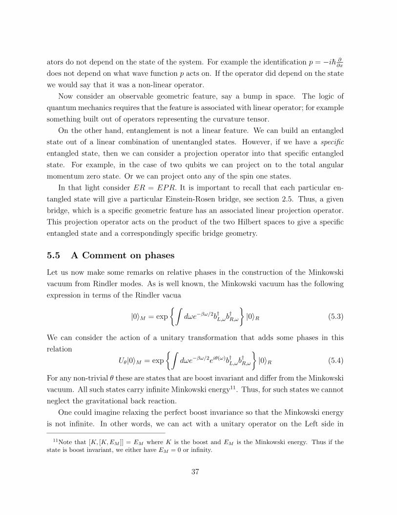
ators do not depend on the state of the system. For example the identification p = −i~ ∂∂x

does not depend on what wave function p acts on. If the operator did depend on the state

we would say that it was a non-linear operator.

Now consider an observable geometric feature, say a bump in space. The logic of

quantum mechanics requires that the feature is associated with linear operator; for example

something built out of operators representing the curvature tensor.

On the other hand, entanglement is not a linear feature. We can build an entangled

state out of a linear combination of unentangled states. However, if we have a specific

entangled state, then we can consider a projection operator into that specific entangled

state. For example, in the case of two qubits we can project on to the total angular

momentum zero state. Or we can project onto any of the spin one states.

In that light consider ER = EPR. It is important to recall that each particular en-

tangled state will give a particular Einstein-Rosen bridge, see section 2.5. Thus, a given

bridge, which is a specific geometric feature has an associated linear projection operator.

This projection operator acts on the product of the two Hilbert spaces to give a specific

entangled state and a correspondingly specific bridge geometry.

5.5 A Comment on phases

Let us now make some remarks on relative phases in the construction of the Minkowski

vacuum from Rindler modes. As is well known, the Minkowski vacuum has the following

expression in terms of the Rindler vacua

|0〉M = exp

∫dωe−βω/2b†L,ωb

†R,ω

|0〉R (5.3)

We can consider the action of a unitary transformation that adds some phases in this

relation

Uθ|0〉M = exp

∫dωe−βω/2eiθ(ω)b†L,ωb

†R,ω

|0〉R (5.4)

For any non-trivial θ these are states that are boost invariant and differ from the Minkowski

vacuum. All such states carry infinite Minkowski energy11. Thus, for such states we cannot

neglect the gravitational back reaction.

One could imagine relaxing the perfect boost invariance so that the Minkowski energy

is not infinite. In other words, we can act with a unitary operator on the Left side in

11Note that [K, [K,EM ]] = EM where K is the boost and EM is the Minkowski energy. Thus if thestate is boost invariant, we either have EM = 0 or infinity.

37

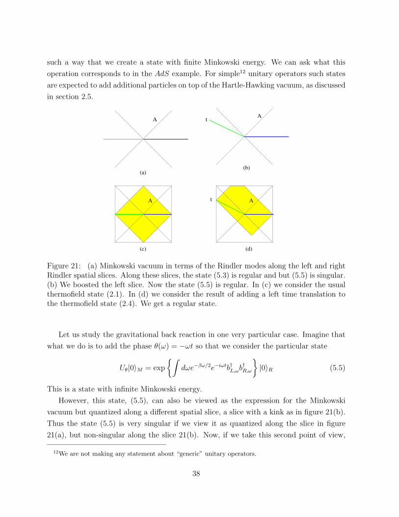
such a way that we create a state with finite Minkowski energy. We can ask what this

operation corresponds to in the AdS example. For simple12 unitary operators such states

are expected to add additional particles on top of the Hartle-Hawking vacuum, as discussed

in section 2.5.

AA

tA A

t

(b)

(d)(c)

(a)

Figure 21: (a) Minkowski vacuum in terms of the Rindler modes along the left and rightRindler spatial slices. Along these slices, the state (5.3) is regular and but (5.5) is singular.(b) We boosted the left slice. Now the state (5.5) is regular. In (c) we consider the usualthermofield state (2.1). In (d) we consider the result of adding a left time translation tothe thermofield state (2.4). We get a regular state.

Let us study the gravitational back reaction in one very particular case. Imagine that

what we do is to add the phase θ(ω) = −ωt so that we consider the particular state

Uθ|0〉M = exp

∫dωe−βω/2e−iωtb†L,ωb

†R,ω

|0〉R (5.5)

This is a state with infinite Minkowski energy.

However, this state, (5.5), can also be viewed as the expression for the Minkowski

vacuum but quantized along a different spatial slice, a slice with a kink as in figure 21(b).

Thus the state (5.5) is very singular if we view it as quantized along the slice in figure

21(a), but non-singular along the slice 21(b). Now, if we take this second point of view,

12We are not making any statement about “generic” unitary operators.

38

we see that an operator in the future, call it A, has a different expression in terms of these

a and a† operators than the one that we have in the usual case, when we quantize along

the usual line, 21(a). So, the same spacetime region has different expressions in terms of

Schrodinger picture operators if we choose one slice vs. the other. Now, here we would

not call this a “state dependence” because we are simply talking about the same abstract

state but with different choices for the parametrization of the operators.

Now, let us return to the case of the two sided AdS black hole. When we do time

evolution on one of the sides we also introduce relative phases between the states of the

left and the right CFT (2.4). But we do not get a singular state in the bulk. The phases

reflect in the bulk by constructing a different bridge, a different region of the black hole

spacetime, see figure 5(c). Interestingly, this different region is such that the state given by

these phases is no longer singular. In some sense, the interior automatically adjusts so that

we are effectively quantizing along the surface with the kink so as to get a non-singular

state. Now we can consider an A operator which is in the interior and that is common

to both regions. The construction of A in terms of Schrodinger picture operators will be

different. But nevertheless A is describing the same spacetime region in the interior.

6 Conclusion

The full Kruskal geometry figure 2 with its two asymptotic regions has a number of inter-

pretations. The most interesting for us is that it represents the geometry of two distant

black holes, which have been created in a certain maximally entangled state. Pair creation

of near-extremal black holes in an external electric field provides an explicit example of

the creation of maximally entangled black holes.

We claim that any pair of entangled black holes will be connected by some kind of

Einstein-Rosen bridge. The Einstein-Rosen bridge is a manifestation of entanglement. We

further suggest that the connection is more general than just black holes, although in most

cases the bridge may not have a smooth geometric interpretation. The general principle

relating Einstein-Rosen bridge and entanglement we summarized by the relation

ER = EPR.

Black holes created by collapse are usually considered to be one-sided. But as a normal

one-sided black hole evaporates it effectively becomes two-sided at the Page time when it

has become maximally entangled with the outgoing radiation. By the ER=EPR principle

it is connected to the outgoing radiation by a complex Einstein-Rosen bridge with many

39

outlets. The outlets connect the bridge to the black hole, and to the radiation quanta. An

observer called Alice can collect the radiation and run it through a quantum computer.

The output will be a second black hole maximally entangled with the first, and therefore

connected to it by a smooth Einstein-Rosen bridge. Here we are ignoring possible limits

of quantum computation [18].

We emphasize that to describe the interior of a maximally entangled black hole we

need to know how it is entangled. We also need to consider the system that the black hole

is entangled with. It is not enough to focus on the microstates of the given black hole.

The interior is constructed from the microstates of the black hole as well as the states of

the system that purifies the black hole in the full Hilbert space. There are many patterns

of entanglement that lead to the same density matrices for the black hole exterior. It is

not enough to know those density matrices; one must know the pattern of entanglement.

Namely, one needs to know the particular entangled state. Even if most entangled states

had firewalls, if a black holes is entangled with a second system in the appropriate way,

the firewalls would dissolve and produce a smooth horizon. This can happen even though

the two systems are far away!.

The argument of AMPS assumes that Alice can distill a particular qubit RB from the

radiation (or from the black hole that Alice has made from the radiation). RB is the qubit

which is maximally entangled with a certain late radiation mode B. After distilling RB

Alice can bring it back to the black hole where she will find that B and RB are maximally

entangled. By the monogamy of entanglement B cannot be entangled with its partner

mode A, on the other side of the horizon. The breaking of the entanglement between A

and B implies the existence of a high energy quantum in the mode A. Alice will be hit by

that quantum as she passes the horizon. We agree with this conclusion and the example

of the entangled black holes showed this clearly.

There are two possible lessons of the AMPS argument. The first is that in the process

of distilling RB, Alice created the particle in the related mode A. If that’s the case there

is no need for a firewall. Alice merely created one high energy particle and found it when

she entered the horizon.

The other possibility is that the high energy particle was present whether or not Alice

distilled RB. If so, there must be a high energy quantum in every A mode, i.e., there is a

firewall.

AMPS argue that Alice could not possibly have created the particle. For one thing the

distillation process took place very far from the black hole, and the particle was detected

just beyond the horizon. The second thing is that the particle was moving in the wrong

40

direction to have arrived from outside the black hole. Thus it must have been there all

along, at least after the Page time. Applying the argument to every A,B pair, AMPS

concludes that there is a firewall.

We argue that this conclusion is incorrect; the high energy particle in the A mode, we

believe, was indeed created by Alice when she distilled RB. If she distills one such mode

she must create at a quantum in the related A mode, but otherwise she leave the horizon

smooth. (Of course it is always possible that a clumsy Alice will accidentally disrupt more

than a single RB and do greater damage to the horizon.)

Moreover, if she does not distill any RB, no particles will be created and the horizon

may be completely smooth. The question is how is it possible that Alice created a particle

moving along the horizon, in mode A, from such a large distance? Our answer is that

the particle arrives at A not from outside the black hole, but through the Einstein-Rosen

bridge. The argument can be made with some confidence in the case where the radiation

has been replaced by a second entangled black hole. The most controlled case in which

the argument can be illustrated is the “laboratory” model of section 4.2. The laboratory

model is based on gauge-gravity duality involving two entangled boundary CFT’s.

It seems to be a good strategy to formulate behind-the-horizon physics in terms of

Wheeler De Witt wave functions. Consider ordinary ADS/CFT gauge-gravity duality.

The bulk dual of a Schrodinger picture wave function in the boundary theory is not an

instantaneous state in the bulk. It is much better to think of it as the Wheeler De Witt

wave function of the whole space-time region obtained by combining all spacelike surfaces

that end at the boundary slice. See figure 22. The WdW wave-function encodes the bulk

in a way that does not depend on slicing.

In the same way, we should not think of an Einstein-Rosen bridge as an instantaneous

configuration. It is a space-time region of the type shown in figures 22, 5, 19, 21(d).

Different types of Einstein-Rosen bridges refer to different types of space-time regions that

end on a particular boundary slice. The bridge between two entangled systems depends

on the particular entangled state that we consider, and not only on the total amount of

entanglement. We believe that similar things are true in the case of black holes connected

to radiation by an Einstein-Rosen bridge.

Regarding the AMPSS paradox, we think that it is important to note that the easy

measurements E, that are performed on the radiation, do not destroy the quantum infor-

mation in the radiation that is entangled with the near horizon qubits. The construction

of the mode operator A from radiation qubits is ambiguous and can be done in many ways.

AMPSS argue that the action of local operators E does not commute with the operators

41

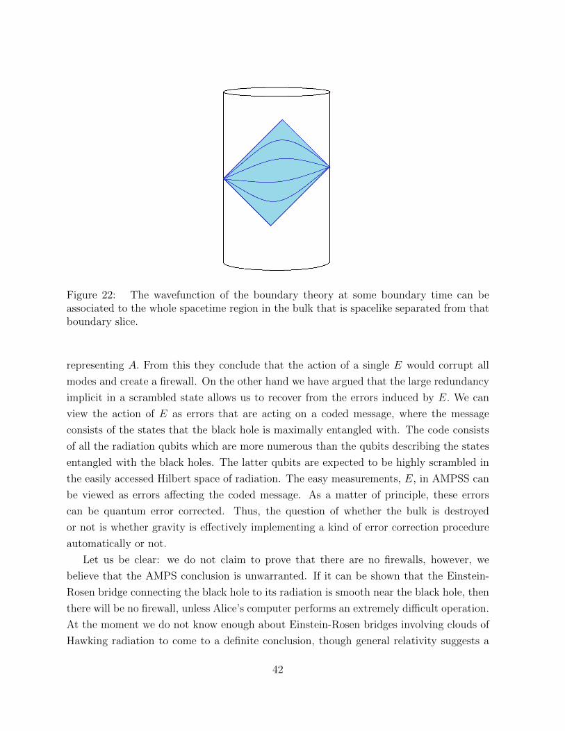
Figure 22: The wavefunction of the boundary theory at some boundary time can beassociated to the whole spacetime region in the bulk that is spacelike separated from thatboundary slice.

representing A. From this they conclude that the action of a single E would corrupt all

modes and create a firewall. On the other hand we have argued that the large redundancy

implicit in a scrambled state allows us to recover from the errors induced by E. We can

view the action of E as errors that are acting on a coded message, where the message

consists of the states that the black hole is maximally entangled with. The code consists

of all the radiation qubits which are more numerous than the qubits describing the states

entangled with the black holes. The latter qubits are expected to be highly scrambled in

the easily accessed Hilbert space of radiation. The easy measurements, E, in AMPSS can

be viewed as errors affecting the coded message. As a matter of principle, these errors

can be quantum error corrected. Thus, the question of whether the bulk is destroyed

or not is whether gravity is effectively implementing a kind of error correction procedure

automatically or not.

Let us be clear: we do not claim to prove that there are no firewalls, however, we

believe that the AMPS conclusion is unwarranted. If it can be shown that the Einstein-

Rosen bridge connecting the black hole to its radiation is smooth near the black hole, then

there will be no firewall, unless Alice’s computer performs an extremely difficult operation.

At the moment we do not know enough about Einstein-Rosen bridges involving clouds of

Hawking radiation to come to a definite conclusion, though general relativity suggests a

42

smooth horizon. However, we claim there is no convincing argument in favor of firewalls.

One thing seems clear: the smoothness of the horizon of an old black hole does depend

on what we do with the radiation. We can always process the radiation to produce the

thermofield double state, which has a smooth horizon. Or the thermofield double plus

extra high energy particles, which do not.

The AMPS paradox is an extremely subtle one whose resolution, we believe, will have

much to teach us about the connection between geometry and entanglement. AMPS

pointed out a deep and genuine paradox about the interior of black holes. Their resolution

was firewalls, but in our view the solution more likely involves Einstein-Rosen bridges.

The interior of an old black hole would be an Einstein-Rosen bridge constructed from the

micro-degrees of freedom of the black hole as well the radiation.

Acknowledgements

We would like to thank N. Arkani Hamed, R. Bousso, D. Harlow, T. Hartman, D. Marolf,

J. Polchinski, S. Shenker, D. Stanford and H. Verlinde for discussions. JM was supported

in part by U.S. Department of Energy grant DE-FG02-90ER40542. LS was supported in

part by NSF under Grant No. PHY11-25915.

A Black hole pair creation in a magnetic field

Here we review some formulas from [19, 20].

The background Melvin solution has the form

ds2 =1

B2

[Λ2b(dt

2 + dz2 + dρ2) +ρ2

Λ2b

dφ2

](A.1)

F =2

BdφdΛ−1b , Λb ≡ 1 +

ρ2

4(A.2)

We have pulled out the parameter B so that the scaling with B is manifest. The instanton

solution has the form

ds2 =1

A2

[Λ2

(x− y)2[−G(y)dτ 2 −G−1(y)dy2 +G−1(x)dx2] +

G(x)

Λ2(x− y)2dφ2

](A.3)

F = dφdΦ (A.4)

G(x) = 1− x2(1 + qAx)2 , Φ =2

ΛB(1 +

1

2qBx) (A.5)

Λ = (1 +1

2qBx)2 +

B2G(x)

4A2(x− y)2(A.6)

43

where q, A and B are parameters obeying qB < 1/4 and a relation written in eqn. (2.9)

of [20]. The function G(x) has four zeros, ζi, i = 1, · · · , 4. We are interested in the regime

where qB 1. In this regime we have that A ∼ B. Then the four roots of the equation

G(x) = 0 are

ζ1 = − 1

qA− 1 + · · · , ζ2 = − 1

qA+ 1 + · · · , ζ3 = −1 + · · · , ζ4 = 1 + · · · (A.7)

We take ζ2 < y < ζ3 < x < ζ4.

In the regime where x and y are of order one, we can approximate the function G(x)

by G(x) = 1− x2 and similarly for G(y). We then define the new variables

ρ2 =(1− x2)(x− y)2

, r2 =y2 − 1

(x− y)2(A.8)

We can also approximate Λ ∼ 1 + (1−x2)4(x−y)2 = 1 + 1

4ρ2. Then the metric (A.3) becomes

identical to (A.1), except that dt2 + dz2 = r2dτ 2 + dr2. In other words, we get the metric

in polar coordinates. These become Rindler coordinates after we analytically continue τ

to Lorentzian time. The overall scale is set by B = A.

This approximate form is correct as long as we are far from y ∼ ζ2 ∼ − 1qA

. In that

region cannot longer approximate G(y) ∼ 1− y2. This region corresponds to r ∼ 1. This

is the region where the black holes are sitting. More precisely, the metric starts deviating

from the Melvin solution (A.1) when r − 1 ∼ qA. In this region, we have

−G(y) = y2(1 + qAy)2 − 1 ∼ y2(1 + qAy)2 (A.9)

where we neglected the 1 since y is large. Since x continues to be of order one, we can still

approximate G(x) ∼ 1− x2. In this regime we can approximate Λ ∼ 1 and (x− y) ∼ −y.

Then the metric (A.3) becomes

ds2 =1

A2

−G(y)

y2dτ 2 − 1

y2G(y)dy2 +

1

y2[

dx2

(1− x2)+ (1− x2)dφ2]

(A.10)

ds2 = (1− q

r)2dτ 2

A2+

dr2

(1− qr)2

+ r2dΩ22 (A.11)

r = − 1

Ay, x = sin θ (A.12)

Thus the x and φ directions give a two sphere and the other dimensions give a black hole

with a Schwarzschild radius equal to q. This black hole is extremal in this approximation.

44

When we go near the horizon of the black hole, it is important to remember the 1 in (A.9)

this replaces

(1− q

r)2 −→ (1− q

r)2 − (qA)2 (A.13)

This splits the two zeros by a small amount, giving the black hole a small amount of

non-extremality.

The condition that set B = A is the same condition that is setting the temperature of

the black hole to be equal to the Rindler acceleration. The circular trajectory of the black

hole is parametrized by the coordinate τ .

When we view this solution as a tunneling solution, we cut the solution across ordi-

nary Euclidean time, so that we produce two black holes and the horizon is entangled

as expected. Of course, we produce the wormhole of the near extremal Reissner Nord-

strom black hole. The Euclidean time circle τ shrinks to zero at two locations, one is the

horizon of the black hole, which corresponds to y = ζ2 and the other corresponds to the

origin of space that corresponds to y = ζ3, or r = 0. In this case the “long” distance

between the two black holes is dlong ∼ 1/A, while the “short” one through the wormhole

is dshort ∼ −q log(qA). For qA 1 we see that the long distance is much longer than the

short one.

The instanton action, as computed by [20], is

e−I = e−πqB e

π2q2 for qB 1 (A.14)

For a fixed magnetic field it is most convenient to create the smallest possible black hole, at

least when qB 1. It turns out that for the full action, we also maximize the probability

for small black holes, see formula (2.14) in [20]. In other words, the q2 entropic-like

enhancement factor never wins over the first factor. One can isolate the entropic factor by

comparing (A.14) with the probability for creating magnetic monopoles [20]. That ratio

contains the entropy factor eSBH = eπq2, which is similar, but not equal, to (A.14) 13. It

is of course, given by the probability of thermally producing them in Rindler space at the

acceleration temperature. Note that, even though we can “naturally” produce them in

this way, we pay a heavy penalty since the tunneling rate is very small.

13The difference is due to Coulomb and Newtonian self interactions of the black hole loop [20].

45

References

[1] A. Einstein, B. Podolsky and N. Rosen, “Can quantum mechanical description of

physical reality be considered complete?,” Phys. Rev. 47, 777 (1935).

[2] A. Einstein and N. Rosen, “The Particle Problem in the General Theory of Relativity,”

Phys. Rev. 48, 73 (1935).

[3] R. W. Fuller and J. A. Wheeler, “Causality and Multiply Connected Space-Time,”

Phys. Rev. 128, 919 (1962).

[4] J. L. Friedman, K. Schleich and D. M. Witt, “Topological censorship,” Phys. Rev.

Lett. 71, 1486 (1993) [Erratum-ibid. 75, 1872 (1995)] [gr-qc/9305017].

[5] G. J. Galloway, K. Schleich, D. M. Witt and E. Woolgar, “Topological censorship and

higher genus black holes,” Phys. Rev. D 60, 104039 (1999) [gr-qc/9902061].

[6] W. Israel, “Thermo field dynamics of black holes,” Phys. Lett. A 57, 107 (1976).

[7] J. M. Maldacena and A. Strominger, “AdS(3) black holes and a stringy exclusion

principle,” JHEP 9812, 005 (1998) [hep-th/9804085].

[8] G. T. Horowitz and D. Marolf, “A New approach to string cosmology,” JHEP 9807,

014 (1998) [hep-th/9805207].

[9] V. Balasubramanian, P. Kraus, A. E. Lawrence and S. P. Trivedi, “Holographic probes

of anti-de Sitter space-times,” Phys. Rev. D 59, 104021 (1999) [hep-th/9808017].

[10] J. M. Maldacena, “Eternal black holes in anti-de Sitter,” JHEP 0304, 021 (2003)

[hep-th/0106112].

[11] A. Almheiri, D. Marolf, J. Polchinski and J. Sully, “Black Holes: Complementarity

or Firewalls?,” arXiv:1207.3123 [hep-th].

[12] A. Almheiri, D. Marolf, J. Polchinski, D. Stanford and J. Sully, “An Apologia for

Firewalls,” arXiv:1304.6483 [hep-th].

[13] S. L. Braunstein, “Black hole entropy as entropy of entanglement, or it’s curtains for

the equivalence principle”, arXiv:0907.1190v1 [quant-ph]. S. L. Braunstein, S. Piran-

dola and K. Z.yczkowski, “Entangled black holes as ciphers of hidden information,”

Phys. Rev. Lett. 110, 101301 (2013) [arXiv:0907.1190 [quant-ph]].

46

[14] S. D. Mathur, “The Information paradox: A Pedagogical introduction,” Class. Quant.

Grav. 26, 224001 (2009) [arXiv:0909.1038 [hep-th]].

[15] S. B. Giddings and Y. Shi, “Quantum information transfer and models for black hole

mechanics,” arXiv:1205.4732 [hep-th].

[16] K. Papadodimas and S. Raju, “An Infalling Observer in AdS/CFT,” arXiv:1211.6767

[hep-th].

[17] S. G. Avery and B. D. Chowdhury, “Firewalls in AdS/CFT,” arXiv:1302.5428 [hep-

th].

[18] D. Harlow and P. Hayden, “Quantum Computation vs. Firewalls,” arXiv:1301.4504

[hep-th].

[19] D. Garfinkle and A. Strominger, “Semiclassical Wheeler wormhole production,” Phys.

Lett. B 256, 146 (1991).

[20] D. Garfinkle, S. B. Giddings and A. Strominger, “Entropy in black hole pair produc-

tion,” Phys. Rev. D 49, 958 (1994) [gr-qc/9306023].

[21] I. Heemskerk, D. Marolf, J. Polchinski and J. Sully, “Bulk and Transhorizon Mea-

surements in AdS/CFT,” JHEP 1210, 165 (2012) [arXiv:1201.3664 [hep-th]].

[22] D. Bak, M. Gutperle and A. Karch, “Time dependent black holes and thermal equi-

libration,” JHEP 0712, 034 (2007) [arXiv:0708.3691 [hep-th]]. D. Bak, M. Gutperle

and S. Hirano, “Three dimensional Janus and time-dependent black holes,” JHEP

0702, 068 (2007) [hep-th/0701108].

[23] S. Ryu and T. Takayanagi, “Holographic derivation of entanglement entropy from

AdS/CFT,” Phys. Rev. Lett. 96, 181602 (2006) [hep-th/0603001].

[24] M. Van Raamsdonk, “Building up spacetime with quantum entanglement,” Gen. Rel.

Grav. 42, 2323 (2010) [Int. J. Mod. Phys. D 19, 2429 (2010)] [arXiv:1005.3035 [hep-

th]].

[25] T. Hartman and J. Maldacena, “Time Evolution of Entanglement Entropy from Black

Hole Interiors,” arXiv:1303.1080 [hep-th].

[26] I. A. Morrison and M. M. Roberts, “Mutual information between thermo-field doubles

and disconnected holographic boundaries,” arXiv:1211.2887 [hep-th].

47

[27] D. Marolf and A. C. Wall, “Eternal Black Holes and Superselection in AdS/CFT,”

Class. Quant. Grav. 30, 025001 (2013) [arXiv:1210.3590 [hep-th]].

[28] D. Marolf, “Black Holes, AdS, and CFTs,” Gen. Rel. Grav. 41, 903 (2009)

[arXiv:0810.4886 [gr-qc]].

[29] A. Sen, “State Operator Correspondence and Entanglement in AdS2/CFT1,” Entropy

13, 1305 (2011) [arXiv:1101.4254 [hep-th]].

[30] D. N. Page, “Average entropy of a subsystem,” Phys. Rev. Lett. 71, 1291 (1993)

[gr-qc/9305007].

D. N. Page, “Information in black hole radiation,” Phys. Rev. Lett. 71, 3743 (1993)

[hep-th/9306083].

[31] L. Susskind, “Black Hole Complementarity and the Harlow-Hayden Conjecture,”

arXiv:1301.4505 [hep-th].

[32] S. H. Shenker and D. Stanford, “Black holes and the butterfly effect,” arXiv:1306.0622

[hep-th].

[33] D. Stanford, private communication. To appear.

[34] P. Hayden and J. Preskill, “Black holes as mirrors: Quantum information in random

subsystems,” JHEP 0709 (2007) 120 [arXiv:0708.4025 [hep-th]].

[35] E. Verlinde and H. Verlinde, “Black Hole Entanglement and Quantum Error Correc-

tion,” arXiv:1211.6913 [hep-th].

[36] P. Hayden, private communication.

[37] J. Preskill, http://www.theory.caltech.edu/people/preskill/ph229/#lecture

[38] B. Swingle, “Constructing holographic spacetimes using entanglement renormaliza-

tion,” arXiv:1209.3304 [hep-th].

[39] J. Polchinski, L. Susskind and N. Toumbas, “Negative energy, superluminosity and

holography,” Phys. Rev. D 60, 084006 (1999) [hep-th/9903228].

48