JPL Publication 04-008

Scientific Impacts of Wind DirectionErrors

W. Timothy Liu, Seung-Bum Kim, Tong Lee, Y. Tony Song, and Wenqing TangJet Propulsion Laboratory, Pasadena, California

Robert AtlasGoddard Space Flight Center, Greenbelt, Maryland

National Aeronautics andSpace Administration

Jet Propulsion LaboratoryCalifornia Institute of TechnologyPasadena, California

May 2004

The research described in this publication was carried out at the Jet Propulsion Laboratory,California Institute of Technology, under contract with the National Aeronautics and Space Administration (NASA). It was supported by NASA’s Ocean Vector Wind Program. A portion of the work was performed at the NASA Goddard Space Flight Center, Greenbelt, Maryland.

iii

ABSTRACT

An assessment on the scientific impact of random errors in wind direction (< 45°)retrieved from space-based observations under weak wind (< 7 m/s) conditions wasmade. Half of the winds over global oceans are below 7 m/s, in their long-termaverages, and these weak winds cover most of the tropical, sub-tropical, and coastaloceans. Introduction of these errors in the semi-daily winds causes, on average, 5%changes of the yearly mean Ekman and Sverdrup volume transports computed directlyfrom the winds, respectively. These poleward movements of water are the mainmechanisms to redistribute heat from the warmer tropical region to the colder high-latitude regions, and they are the major manifestations of the ocean’s function inmodifying Earth’s climate. Simulation by an ocean general circulation model shows thatthe wind errors introduce a 5% error in the meridional heat transport at tropical latitudes.The simulation also shows that the erroneous winds cause a pile-up of warm surfacewater in the eastern tropical Pacific, similar to the conditions during El Niño episode.Similar wind directional errors cause significant change in sea-surface temperature andsea-level patterns in coastal oceans in a coastal model simulation. Previous studies haveshown that assimilation of scatterometer winds improves 3–5 day weather forecasts in theSouthern Hemisphere. When directional information below 7 m/s was withheld,approximately 40% of the improvement was lost.

ACKNOWLEDGMENTS

Yunjin Kim and Victor Zlotnicki of Jet Propulsion Laboratory first articulated the need ofthis study.

v

TABLE OF CONTENTS

Section 1. Introduction .................................................................................................... 1

Section 2. Distribution of Winds Under Threshold .......................................................... 2

Section 3. Global Ocean Response .................................................................................. 5

Section 4. Coastal Ocean Response ............................................................................... 13

Section 5. Numerical Weather Prediction ...................................................................... 16

Section 6. Discussion .................................................................................................... 17

1

Section 1. Introduction

Even for the proven technique of scatterometry, the accuracy of retrieving vector winds isdegraded below a wind-speed threshold of about 2–3 m/s (e.g., Freilich, 1999; Plant,2000). The threshold appears to be much higher for the experimental technique ofpolarimetric radiometry. The United States Windsat/Coriolis mission, launched inJanuary 2003, was the first instrument designed to demonstrate the polarimetricradiometer approach for acquiring accurate, all-weather measurements of surface vectorwinds from space. It will serve as a risk reduction program for the Conical MicrowaveImager Sounder (CMIS) to operate on the National Polar-orbiting OperationalEnvironmental Satellite System (NPOESS). The prelaunch aircraft flight experimentsdemonstrated appreciable wind direction signals for moderate and high winds (> 7 m/s),but also indicated insufficient sensitivity to wind direction for lighter winds (below 7m/s) at Windsat incident angles (e.g., Yueh et al., 1999).

This is a report on the potential scientific impacts caused by anticipated errors in winddirection. To understand the amount and location of winds under the threshold, thedistribution of the mean and variability of winds over global ocean computed byWenqing Tang is described in Section 2. The wind data used in the ocean studies aredescribed in Section 3.1.

Ocean affects climate mainly by storing solar heating during the warmer seasons andreleasing it in colder seasons and by moving the heat from the warm ocean in lowlatitudes to the cooler oceans in high latitudes. Zonal redistribution of heat in the oceanmixed layer, caused by the relaxation of the trade winds in the equatorial Pacific, alsocauses the major climate episodes of El Niño and La Niña. The meridional redistributionof heat is accomplished through wind-driven Ekman and Sverdrup transport, the impactof which, as computed by Seung-Bum Kim, is described in Section 3.2. Through anocean general circulation model (OGCM), Tong Lee simulated the sea surfacetemperature and surface dynamic topography and the impact on meridional heat transportand zonal heat distribution in the tropical ocean; his results are presented in Section 3.3.Large portions of the population lives near the coast, and coastal oceans are the mostproductive parts of the global oceans. Coastal oceans are known to be more sensitive tosurface forcing than open oceans because the momentum and energy from theatmosphere are absorbed by relatively small volumes of shallow water. The impact of acoastal ocean simulated by a coastal model by Tony Song is described in Section 4.Weather affects our daily lives and the impact in global numerical weather prediction byRobert Atlas is explained in Section 5.

2

Section 2. Distribution of Winds Under Threshold

Figure 1, based on 4 years of daily-gridded ocean wind vector measurements fromSeptember 1999 to August 2003, is derived from the NASA’s QuikSCAT scatterometerand shows that half of winds blowing over the global ocean are under 7 m/s, and a fourthare under 5 m/s. In general, the wind speeds derived from Special Sensor MicrowaveImager may have slightly higher values and those from the scatterometers on Europeanremote sensing satellites may have slightly lower values than QuikSCAT measurements,while the numerical weather prediction (NWP) products of the National Center forEnvironmental Prediction (NCEP) have good agreement with QuikSCAT measurements.It is clear from Figure 2 that the average wind speeds are below 5 m/s for most of thetropical and coastal oceans. The subtropical oceans will also be included if the thresholdis moved up to 7 m/s.

Figure 1. Percentage wind distribution derived from four years (September1999 – August 2003) of measurements by QuikSCAT. The cumulativepercentage of winds falling within certain ranges are also shown.

3

The variability is also low over tropical and subtropical oceans, as shown in Figure 3.The variability is higher in the storm tracks of North Pacific, North Atlantic, and theRoaring Fifties (over the circumpolar currents around Antarctica). The winds in theseregions are strongest in their respective winter season. Much of the increase in root-mean-square deviations is due to these higher seasonal changes in high latitudes. Highwinds are usually transient and require high resolution (temporal and spatial).

Figure 2. Averaged wind speed derived from four years (September 1999 toAugust 2003) of QuikSCAT data. Isotach interval is in 1 m/s. Those for 5, 7, and10 m/s are thickened.

4

Figure 3. Root-mean-square deviation from the 4-year mean derived from dailywinds from QuikSCAT. Isotachs are in m/s.

5

Section 3. Global Ocean Response

3.1 Wind Forcing

The wind data used in the oceanographic studies (described in Sections 3.2, 3.3, and 4)are obtained from the monthly averages of NCEP reanalysis fields for 2000. Thedirection error is modeled to be random and to have a white spectrum. The size of theerror is at the maximum of ± 45° of the NCEP wind direction. Only if the wind speed isless than 7 m/s is the random error introduced. The introduction of directional wind errorwas performed to the 12-hourly wind field instead of time mean.

3.2 Ekman and Svedrup Transports

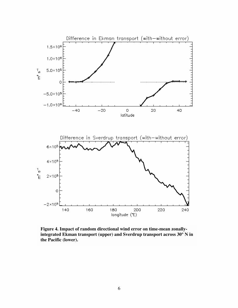
Ekman transport, which is the poleward transport of water near the ocean surface drivenby winds, and Sverdrup transport, which is the poleward transport integrated over theocean depth caused by wind-driven ocean circulation, are functions of a surface windvector. They are computed from the wind fields described in Section 3.1. The Ekmantransport is computed at 5° intervals from 10° to 45° in both hemispheres. Between 10°Sand 10° N, the Coriolis force approaches zero, resulting in the singularity. The randomdirection error perturbs the Ekman transport by about 5% (Figure 4) at 10° N and 10° S.The perturbation is largest at 10° in both hemispheres and becomes smaller towards thehigher latitudes. This latitudinal dependence arises because the wind stress tends to begreater in the subtropics than in the tropics. The size of the perturbation in the Ekmantransport is very close to that in the zonal wind stress, since the relationship between theEkman transport and the wind stress is linear.

6

Figure 4. Impact of random directional wind error on time-mean zonally-integrated Ekman transport (upper) and Sverdrup transport across 30° N inthe Pacific (lower).

7

It is interesting to observe that the absolute magnitude of the Ekman transport alwaysdecreases due to the random direction wind error. The reason is that the wind direction ispredominantly zonal in the tropics where most of the perturbation occurs; therefore, theerror acts to reduce the zonal wind speed even if the direction error is random.

The Sverdrup transport is computed by integrating the transport at one point, between theeastern and western boundaries of the oceans. In the subtropical gyre (between about 15°and 45° in latitude in both hemispheres), the directional error reduces the strength of thewind-driven gyre because of the weakening westerlies at around 45° and easterlies ataround 15°. This reduction appears as positive and negative anomalies in the Northernand Southern Hemispheres respectively (Figure 5). The error in the zonal wind stress ismore positive near 5° N than at 15° N due to more frequent perturbation at lowerlatitudes (Figure 7). This results in the positive perturbation in Sverdrup transportbetween 5° N and 15° N.

Figure 5. Impact of random directional wind error on time-mean zonally-integrated Sverdrup transport.

8

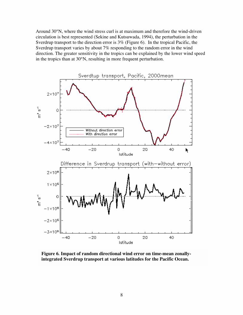
Around 30°N, where the wind stress curl is at maximum and therefore the wind-drivencirculation is best represented (Sekine and Kutsuwada, 1994), the perturbation in theSverdrup transport to the direction error is 3% (Figure 6). In the tropical Pacific, theSverdrup transport varies by about 7% responding to the random error in the winddirection. The greater sensitivity in the tropics can be explained by the lower wind speedin the tropics than at 30°N, resulting in more frequent perturbation.

Figure 6. Impact of random directional wind error on time-mean zonally-integrated Sverdrup transport at various latitudes for the Pacific Ocean.

9

3.3 Simulation of Ocean’s Response by OGCM

A global OCGM is used to evaluate the impact of random errors in the direction of weakwind (< 7 m/s). The model is the same as that used by Lee et al. (2002) to study theimpact of the Indonesian throughflow on ocean circulation. Briefly, it is a version of theMIT OGCM (Marshall et al. 1997a) with a horizontal resolution of 1º × 0.3º in thetropics and 1º × 1º in the extratropics. There are 46 vertical levels with a depthincrement ranging from 10 m above 150 m to intervals of 400 m at depth. Two advancedmixing schemes are employed: the so-called K-Profile Parameterization (KPP) verticalmixing (Large et al., 1994) and the GM isopycnal mixing (Gent and McWilliams, 1990).The model is forced at the surface by 12-hourly wind stress and by daily heat andfreshwater fluxes obtained from the NCEP reanalysis (Kalnay et al., 1996).

The control and pertubation experiment are both one-year integrations (year 2000) forcedby winds described in Section 3.1, with and without random directional errors.Figure 7 shows the difference in zonal wind stress with and without introducing therandom directional error (upper panel). The random directional noises result in a westerlybias in the time-mean zonal wind in the tropical Pacific and Atlantic Ocean. This isbecause the wind over these regions is predominantly weak easterly wind. Therefore,any error in direction would cause a reduction of the easterly (i.e., introducing a westerlybias). The fact that a mid-latitude westerly has little bias is because wind is generallystrong there and so little directional error perturbation is applied.

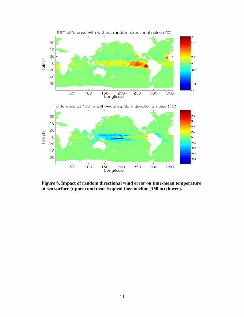
The lower panel of Figure 7 shows the impact of the directional wind error at sea level.The biased westerly in the perturbed wind causes the sea level to pile up in the easternequatorial Pacific and Atlantic. The opposite is true for the equatorial Indian Oceanbecause the perturbed wind is more easterly (the mean wind is westerly there). Figure 8shows the impact of the directional wind error on simulated temperature at sea surfaceand the near tropical thermocline (150 m). A bias of about 1º C is seen in the easternequatorial Pacific cold tongue region because the biased wind (more westerly) suppressesupwelling there by depressing the thermocline. The opposite is true off the westernequatorial Pacific because thermocline is being lifted up. The 1º C bias in the cold tongueregion is quite substantial because it is as large as the threshold of anomalous temperaturefor that region that is used to define an El Niño.

10

Figure 7. Impact of random directional wind error on time-mean zonal wind(upper) and sea level (lower).

11

Figure 8. Impact of random directional wind error on time-mean temperatureat sea surface (upper) and near tropical thermocline (150 m) (lower).

12

Figure 9 shows the impact on the meridional transport stream function (upper panel) andon meridional heat transport (lower panel), both integrated zonally around the globe. Themeridional overturning circulation and poleward heat transport in the equatorial regionare reduced by about 5% due to the random directional wind error.

Figure 9. Impact of random directional wind error on time-mean meridionaltransport streamfunction (upper) and poleward heat transport (lower).

13

Section 4. Coastal Ocean Response

The coastal modeling experiments are based on the Regional Ocean Model System(ROMS), an evolution of the S-Coordinate Rutgers University Model (SCRUM),originally developed by Song & Haidvogel (1994). Similar to SCRUM, ROMS is aconservative, finite-volume discretization of the hydrostatic primitive equations inboundary-following coordinates with a variable free surface, Jacobian schemes for thepressure terms (Song, 1998), and includes new features of high-order upstream-biasedadvection, KPP mixing, and parallel computing capabilities (Shchepetkin & McWilliams,2001). This model has been shown particularly suitable for coastal studies (e.g.,Marchesiello et al., 2001).

Several other community ocean models are also available, including Modular OceanModel (MOM) (Bryan, 1969), Miami Isopycnic-Coordinate Ocean Model (MICOM)(Bleck & Chassignet, 1994), Princeton Ocean Model (POM) (Blumberg & Mellor, 1987),and MIT model (Marshall et al., 1997b). Each of these models has its distinct advantagesdepending on specific applications. However, we have demonstrated expertise andexperience with ROMS. In particular, several coastal and basin-scale models based onROMS have been established on JPL’s supercomputers. Based on these coastal andbasin-scale models, we have developed a set of nested high-resolution coastal models forthe United States West Coast in particular for this study.

Our basin-scale model is the Pacific Ocean with a horizontal resolution of a 0.5º × 0.5ºcovering the area from 45° S to 65° N and 100° E to 70° W. The water depth is dividedinto 20 topography-following levels, with a minimum depth of 50 m near the coastal walland a maximum depth of 5500 m in the deep ocean. The model starts with the initialconditions of annual mean temperature and salinity [Levitus et al., 1994]. The surfaceforcing are monthly mean air-sea fluxes of momentum, heat, and freshwater fromNCEP/NCAR reanalysis. For the heat and salt flux, a thermal feedback term is applied.The model is first spun-up for 30 years with the annual-mean forcing, and then integratedfrom year 1948 to year 2003 by monthly-mean forcing. This basin-scale model providesopen boundary conditions for our high-resolution United States West Coast model.

Our high-resolution United States West Coast model extends in latitude from 30º N to48º N following the United States West Coastline. Using orthogonal curvilinearcoordinates, the coastal region is divided into 480 × 520 grid cells, with an average gridsize of 5 × 5 km. Such a fine-grid is necessary for resolving coastal features such asupwelling fronts, filaments, and eddies, as will be shown later. Although some of thecoastal processes we will examine are internally driven and can be modeled regionally,most are driven by some combination of local and remote forcing. Therefore, the coastalmodel is nested into the Pacific Ocean model to offer a compromise for obtaining high-resolution in the coastal regions of interest and minimizing the overall computationalcoast, without losing the influence of the large-scale dynamics. The coastal model is runfor 10 years (1991–2000) to reach a quasi-equilibrium state.

14

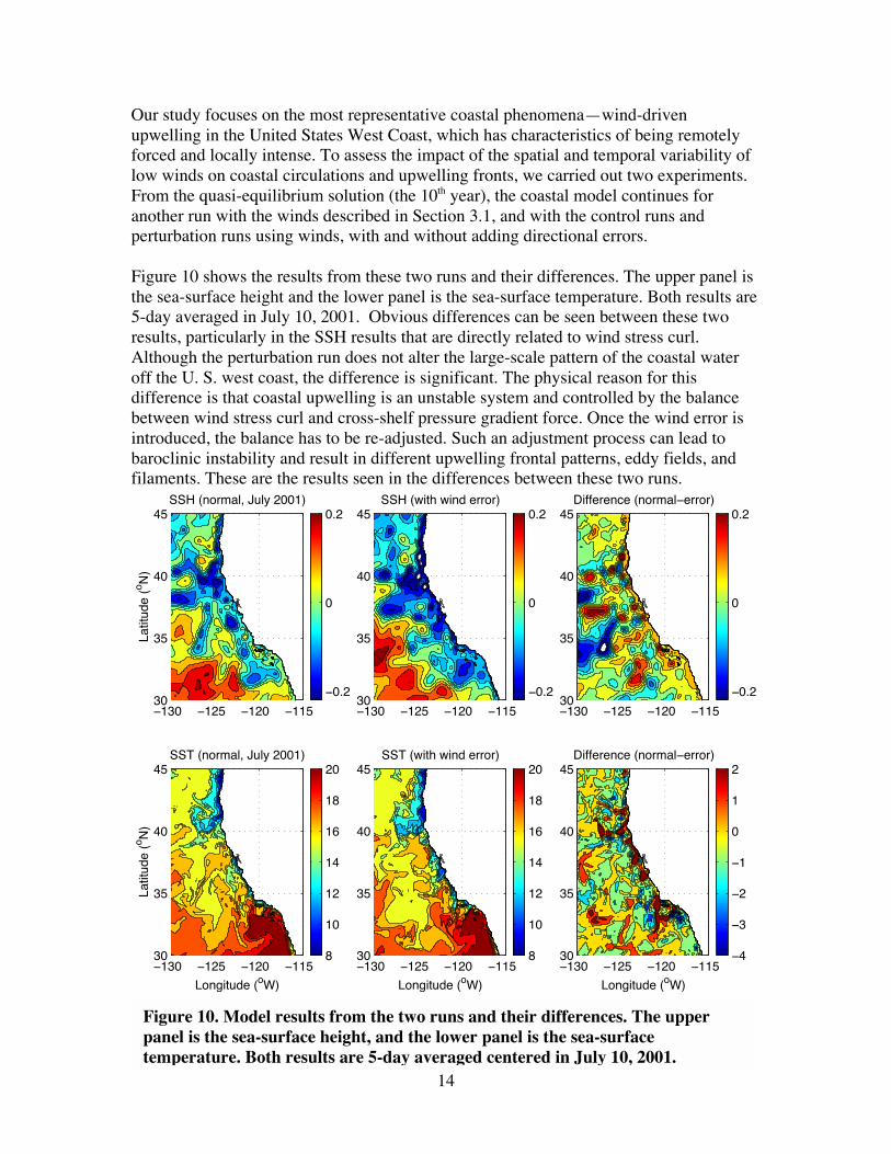
Our study focuses on the most representative coastal phenomena—wind-drivenupwelling in the United States West Coast, which has characteristics of being remotelyforced and locally intense. To assess the impact of the spatial and temporal variability oflow winds on coastal circulations and upwelling fronts, we carried out two experiments.From the quasi-equilibrium solution (the 10th year), the coastal model continues foranother run with the winds described in Section 3.1, and with the control runs andperturbation runs using winds, with and without adding directional errors.

Figure 10 shows the results from these two runs and their differences. The upper panel isthe sea-surface height and the lower panel is the sea-surface temperature. Both results are5-day averaged in July 10, 2001. Obvious differences can be seen between these tworesults, particularly in the SSH results that are directly related to wind stress curl.Although the perturbation run does not alter the large-scale pattern of the coastal wateroff the U. S. west coast, the difference is significant. The physical reason for thisdifference is that coastal upwelling is an unstable system and controlled by the balancebetween wind stress curl and cross-shelf pressure gradient force. Once the wind error isintroduced, the balance has to be re-adjusted. Such an adjustment process can lead tobaroclinic instability and result in different upwelling frontal patterns, eddy fields, andfilaments. These are the results seen in the differences between these two runs.

−0.2

0

0.2

−130 −125 −120 −11530

35

40

45

Latit

ude

(o N)

SSH (normal, July 2001)

−0.2

0

0.2

−130 −125 −120 −11530

35

40

45SSH (with wind error)

−0.2

0

0.2

−130 −125 −120 −11530

35

40

45Difference (normal−error)

8

10

12

14

16

18

20

−130 −125 −120 −11530

35

40

45

Longitude (oW)

Latit

ude

(o N)

SST (normal, July 2001)

8

10

12

14

16

18

20

−130 −125 −120 −11530

35

40

45

Longitude (oW)

SST (with wind error)

−4

−3

−2

−1

0

1

2

−130 −125 −120 −11530

35

40

45

Longitude (oW)

Difference (normal−error)

Figure 10. Model results from the two runs and their differences. The upperpanel is the sea-surface height, and the lower panel is the sea-surfacetemperature. Both results are 5-day averaged centered in July 10, 2001.

15

Figure 11. Forecast skill in Southern Hemisphere; black-control; green-SeaWinds, and red-perturbation.

16

Section 5. Numerical Weather Prediction

The Geosynchronous Earth Orbit Satellite (GEOS-4) data assimilation system, which isoperational at NASA/GSFC was used to estimate the impact of directional errors onnumerical weather prediction. GEOS-4 consists of the fvGCM (Finite Volume GeneralCirculation Model) and PSAS (Physical Space statistical Analysis System). For theexperiments described below, data assimilation was performed for the period of April 10,2003 – May 15, 2003. The data assimilation experiments were each followed by a seriesof 26 five-day forecasts, starting on April 15 and running every day. Three experimentswere conducted:

• “Control” run (includes no satellite surface winds used, but the full complementof operationally-used observational data);

• “SeaWinds” experiment (includes adds surface vector winds from SeaWinds onQuikSCAT to the “control”);

• “Perturbation” run (includes “control” and SeaWinds data but with directioninformation removed from winds at or under 7 m/s).

In the PSAS analysis wind vectors above the surface layer of the atmosphere are usedin a three-dimensional multivariate (wind/mass) analysis scheme. These windvectors are computed from the scatterometer surface wind observations accordingto Monin-Obukhov similarity theory. Other (ship and buoy) surface windobservations are used the same way.

The results of the three experiments are shown in Figure 11. Anomaly correlation resultsrepresent the average of the 26 forecasts for each of the experiments. Anomalycorrelation is an important measure of a forecast performance. It represents thecorrelation between forecast and observed departures from a mean climate state, and is asensitive measure of differences in the pattern between forecast and observed fields. Thegreen curve (“SeaWinds”) shows that adding scatterometer winds improves both the skilland the prediction period over the black curve (“control”), while the red curve(“perturbation”) shows that part of this improvement is lost when the directionalinformation for wind speed under threshold is removed. The impact loss varies from41% – 46% for 3–4 day forecasts.

17

Section 6. Discussion

We used constructed winds to illuminate the significance of accurate wind directionmeasurements under weak wind conditions. The percentage change in the anomalycorrection in NWP, the Ekman and Sverdrup transports are, as expected, small becausethey are integrated over global oceans or across ocean basins. Yet, their impact on ourcharacterizing and understanding of weather and climate changes may still be verysignificant. The strong impact in tropical oceans where the trade wind dominates isclearly evident. The impact on NWP is significant in the 3–4 day forecast range.

18

REFERENCES

Bleck, R. and E. P. Chassignet, 1994: “Simulating the oceanic circulation with isopycnic-coordinate models,” The Oceans, Majmdar et al. (eds.), The Pennsylvania Academyof Science, pp. 17-39.

Blumberg, A. F., and G. L. Mellor, 1987: “A description of a three-dimensional coastalocean circulation model,” Vol. 4, Three-Dimensional Coastal Ocean Models. N.Heaps (ed.), AGU, 208 pp.

Freilich, M. and R.S. Dunbar, 1999: “The accuracy of the NSCAT 1 vector winds:comparisons with National Data Buoy center buoys,” J. Geophys. Res., 104(C3),11,231–11,246,.

Gent, P. and J. McWilliams, 1990: “Isopycnal mixing in ocean circulation models,” J.Phys. Oceanogr., 20, 150–155.

Kalnay, E., M. Kanamitsu, R. Kistler, et al., 1996: “The NCEP/NCAR 40-year reanalysisproject,” Bull. Amer. Meteorol. Soc., 77, 437–471.

Large, W.G., J.C. McWilliams, S.C. Doney, 1994: “Oceanic vertical mixing: a reviewand a model with a non local boundary layer parameterization,” Rev. Geophys.,363–403.

Lee, T., I. Fukumori, D. Menemenlis, Z. Xing, and L.-L. Fu, 2002: “Effects of theIndonesian throughflow on the Pacific and Indian Oceans,” J. Phys. Oceanogr., 32,1404–1429.

Levitus, S., R. Burget, and T. Boyer, 1994: “World Ocean Altas: Salinity andTemperature 3–4,” NOAA Altas NESDID, U. S. Dept. Commerce.

Marchesiello, P., J. C. McWilliams, and A. Shchepetkin, 2003: “Equilibrium structureand dynamics of the California current system,” J. Phys. Oceanogr. 33. 753-783.

Marshall, J., A. Adcroft, C. Hill, L. Perelman, and C. Heisey, 1997a: “A finite-volume,incompressible Navier-Stokes model for studies of the ocean on parallel computers,”J. Geophys. Res., 102, 5753–5766.

Marshall, J., C. Hill, L. Perelman, and A. Adcroft, 1997b: “Hydrostatic, quasi-hydrostaticand non-hydrostatic ocean modeling,” J. Geophys. Res., 102, 5733–5752.

Plant, W.J., 2000: “Effects of wind variability on scatterometry at low wind speeds,” J.Geophys. Res., 105, 16,899–16,910.

Roemmich, D. and C. Wunsch, 1985: “Two transatlantic sections: meridional circulationand heat flux in the subtropical North Atlantic Ocean,” Deep Sea Res., 32, 619–664.

Sekine, Y. and K. Kutsuwada, 1994: “Seasonal variation in volumen transport of theKuroshio south of Japan,” J. Phys. Oceanogr., 24, 261–272.

Shchepetkin, A. F., and J. C. McWilliams, 2001: “The regional ocean modeling system: asplit-explicit, free-surface, topography-following coordinate ocean model,” UCLA,31pp.

Song, Y. T., and D. B. Haidvogel, 1994: “A semi-implicit ocean circulation model usinga generalized topography-following coordinate,” J. Comput. Phys., 115, 228–244.

19

Song, Y. T., 1998: “A general pressure gradient formulation for ocean models. Part I:Scheme design and diagnostic analysis,” Mon. Wea. Rev,. 126, 3212–3230.

Yueh, S.H., W.J. Wilson, S.J. Dinardo, F.K.Li, 1999: “Polarimetric microwavebrightness signatures of ocean wind directions,” IEEE Trans. Geosci. RemoteSensing, 37(2), 949–959.