Journal of Urban Economics 76 (2013) 1–14

Contents lists available at SciVerse ScienceDirect

Journal of Urban Economics

www.elsevier .com/locate / jue

City size, network structure and traffic congestion

Theodore Tsekeris a,⇑, Nikolas Geroliminis b

a Centre of Planning and Economic Research (KEPE), 11 Amerikis, 10672 Athens, Greeceb Urban Transport Systems Laboratory (LUTS), École Polytechnique Fédérale de Lausanne (EPFL), Room GC C2 389, Station 18, CH-1015 Lausanne, Switzerland

a r t i c l e i n f o a b s t r a c t

Article history:Received 9 June 2011Revised 20 December 2012Available online 1 February 2013

JEL classification:L9R1R3R4

Keywords:City sizeLand useTransport networkTraffic congestion dynamicsMacroscopic fundamental diagram

0094-1190/$ - see front matter � 2013 Elsevier Inc. Ahttp://dx.doi.org/10.1016/j.jue.2013.01.002

⇑ Corresponding author.E-mail addresses: tsek@kepe.gr (T. Tsekeris), ni

Geroliminis).

This paper presents an alternative approach for analyzing the relationship between land use and trafficcongestion by employing the Macroscopic Fundamental Diagram (MFD). The MFD is an empiricallyobserved relationship between traffic flow and traffic density at the level of an urban region, includinghypercongestion, where flow decreases as density increases. This approach is consistent with the physicsof traffic and allows the parsimonious modeling of intra-day traffic dynamics and their connection withcity size, land use and network characteristics. The MFD can accurately measure the inefficiency of landand network resource allocation due to hypercongestion, in contrast with existing models of congestion.The findings reinforce the ‘compact city’ hypothesis, by favoring a larger mixed-use core area with greaterzone width, block density and number of lanes, compared to the peripheral area. They also suggest a newset of policies, including the optimization of perimeter controls and the fraction of land for transport,which constitute robust second-best optimal strategies that can further reduce congestion externalities.

� 2013 Elsevier Inc. All rights reserved.

1. Introduction

The increasing economic and environmental concerns raised bythe growth of private vehicle use in urban areas have resulted inthe design and implementation of a number of planning and man-agement strategies on the supply side (control of traffic signals,ramp metering, capacity enhancement, etc.) or the demand side(congestion pricing, parking restriction, etc.) to diminish efficiencylosses. From the planning perspective, policies have favored morecompact development patterns by revitalizing the city center andrestricting urban sprawl, through density and boundary growthcontrols (Anas et al., 1998; McConnell et al., 2006). In this context,the appropriate selection of network design parameters is crucialfor the efficient allocation of road investment in the early stagesof planning, or when updating the urban master plan. Such designparameters may encompass the number of road links, average linklength, block area and average number of lanes. Particularly, thequestion of the allocation of resources to large urban clusters ormore spatially dispersed metropolitan areas is critical for the

ll rights reserved.

kolas.geroliminis@epfl.ch (N.

development of countries with a rapidly growing urban popula-tion, such as China and India (Henderson, 2010).

The proper modeling, interpretation and treatment of the rela-tionship between urban land use and congestion are necessary toaddress the above question. However, existing traffic models in ur-ban economics pose severe theoretical and empirical limitations inrealistic applications. This is because they employ link travel costfunctions which cannot accurately specify the intra-day trafficdynamics and relate them to land use and urban-scale networkcharacteristics in a way that is computationally tractable and con-sistent with the physics of traffic. This failure hinders the ability ofeconomic models to support accurate and robust design proposalsfor the allocation of urban land and network resources to diminishcongestion externalities.

Specifically, the traditional models of congestion simplisticallyassume that the travel time on each link is separable and monoton-ically increasing with link flow. This assumption is adopted by theBureau of Public Roads (Branston, 1976) and the Vickrey conges-tion function. The form of such travel time functions implies theexistence of a stationary traffic equilibrium regime and steady-state volume-delay relationships. Several studies have challengedthe use of these functions because of the need to account for thenon-monotonicity of travel time with traffic flow (McDonaldet al., 1999) and showed the intrinsic inconsistency, infeasibility

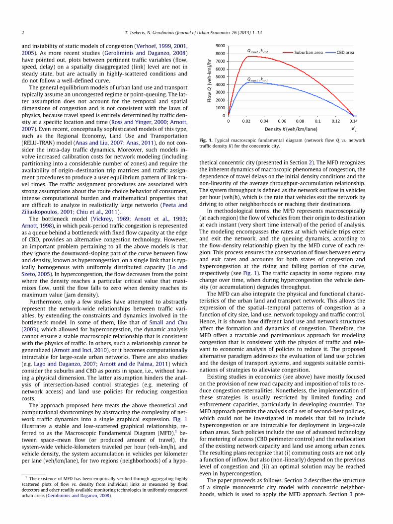
Fig. 1. Typical macroscopic fundamental diagram (network flow Q vs. networktraffic density K) for the concentric city.

2 T. Tsekeris, N. Geroliminis / Journal of Urban Economics 76 (2013) 1–14

and instability of static models of congestion (Verhoef, 1999, 2001,2005). As more recent studies (Geroliminis and Daganzo, 2008)have pointed out, plots between pertinent traffic variables (flow,speed, delay) on a spatially disaggregated (link) level are not insteady state, but are actually in highly-scattered conditions anddo not follow a well-defined curve.

The general equilibrium models of urban land use and transporttypically assume an uncongested regime or point-queuing. The lat-ter assumption does not account for the temporal and spatialdimensions of congestion and is not consistent with the laws ofphysics, because travel speed is entirely determined by traffic den-sity at a specific location and time (Ross and Yinger, 2000; Arnott,2007). Even recent, conceptually sophisticated models of this type,such as the Regional Economy, Land Use and Transportation(RELU-TRAN) model (Anas and Liu, 2007; Anas, 2011), do not con-sider the intra-day traffic dynamics. Moreover, such models in-volve increased calibration costs for network modeling (includingpartitioning into a considerable number of zones) and require theavailability of origin–destination trip matrices and traffic assign-ment procedures to produce a user equilibrium pattern of link tra-vel times. The traffic assignment procedures are associated withstrong assumptions about the route choice behavior of consumers,intense computational burden and mathematical properties thatare difficult to analyze in realistically large networks (Peeta andZiliaskopoulos, 2001; Chiu et al., 2011).

The bottleneck model (Vickrey, 1969; Arnott et al., 1993;Arnott, 1998), in which peak-period traffic congestion is representedas a queue behind a bottleneck with fixed flow capacity at the edgeof CBD, provides an alternative congestion technology. However,an important problem pertaining to all the above models is thatthey ignore the downward-sloping part of the curve between flowand density, known as hypercongestion, on a single link that is typ-ically homogenous with uniformly distributed capacity (Lo andSzeto, 2005). In hypercongestion, the flow decreases from the pointwhere the density reaches a particular critical value that maxi-mizes flow, until the flow falls to zero when density reaches itsmaximum value (jam density).

Furthermore, only a few studies have attempted to abstractlyrepresent the network-wide relationships between traffic vari-ables, by extending the constraints and dynamics involved in thebottleneck model. In some of them, like that of Small and Chu(2003), which allowed for hypercongestion, the dynamic analysiscannot ensure a stable macroscopic relationship that is consistentwith the physics of traffic. In others, such a relationship cannot begeneralized (Arnott and Inci, 2010), or it becomes computationallyintractable for large-scale urban networks. There are also studies(e.g. Lago and Daganzo, 2007; Arnott and de Palma, 2011) whichconsider the suburbs and CBD as points in space, i.e., without hav-ing a physical dimension. The latter assumption hinders the anal-ysis of intersection-based control strategies (e.g. metering ofnetwork access) and land use policies for reducing congestioncosts.

The approach proposed here treats the above theoretical andcomputational shortcomings by abstracting the complexity of net-work traffic dynamics into a single graphical expression. Fig. 1illustrates a stable and low-scattered graphical relationship, re-ferred to as the Macroscopic Fundamental Diagram (MFD),1 be-tween space–mean flow (or produced amount of travel), thesystem-wide vehicle-kilometers traveled per hour (veh-km/h), andvehicle density, the system accumulation in vehicles per kilometerper lane (veh/km/lane), for two regions (neighborhoods) of a hypo-

1 The existence of MFD has been empirically verified through aggregating highlyscattered plots of flow vs. density from individual links as measured by fixeddetectors and other readily available monitoring technologies in uniformly congestedurban areas (Geroliminis and Daganzo, 2008).

thetical concentric city (presented in Section 2). The MFD recognizesthe inherent dynamics of macroscopic phenomena of congestion, thedependence of travel delays on the initial density conditions and thenon-linearity of the average throughput-accumulation relationship.The system throughput is defined as the network outflow in vehiclesper hour (veh/h), which is the rate that vehicles exit the network bydriving to other neighborhoods or reaching their destinations.

In methodological terms, the MFD represents macroscopically(at each region) the flow of vehicles from their origin to destinationat each instant (very short time interval) of the period of analysis.The modeling encompasses the rates at which vehicle trips enterand exit the network, and the queuing dynamics, according tothe flow-density relationship given by the MFD curve of each re-gion. This process ensures the conservation of flows between entryand exit rates and accounts for both states of congestion andhypercongestion at the rising and falling portion of the curve,respectively (see Fig. 1). The traffic capacity in some regions maychange over time, when during hypercongestion the vehicle den-sity (or accumulation) degrades throughput.

The MFD can also integrate the physical and functional charac-teristics of the urban land and transport network. This allows theexpression of the spatial–temporal patterns of congestion as afunction of city size, land use, network topology and traffic control.Hence, it is shown how different land use and network structuresaffect the formation and dynamics of congestion. Therefore, theMFD offers a tractable and parsimonious approach for modelingcongestion that is consistent with the physics of traffic and rele-vant to economic analysis of policies to reduce it. The proposedalternative paradigm addresses the evaluation of land use policiesand the design of transport systems, and suggests suitable combi-nations of strategies to alleviate congestion.

Existing studies in economics (see above) have mostly focusedon the provision of new road capacity and imposition of tolls to re-duce congestion externalities. Nonetheless, the implementation ofthese strategies is usually restricted by limited funding andenforcement capacities, particularly in developing countries. TheMFD approach permits the analysis of a set of second-best policies,which could not be investigated in models that fail to includehypercongestion or are intractable for deployment in large-scaleurban areas. Such policies include the use of advanced technologyfor metering of access (CBD perimeter control) and the reallocationof the existing network capacity and land use among urban zones.The resulting plans recognize that (i) commuting costs are not onlya function of inflow, but also (non-linearly) depend on the previouslevel of congestion and (ii) an optimal solution may be reachedeven in hypercongestion.

The paper proceeds as follows. Section 2 describes the structureof a simple monocentric city model with concentric neighbor-hoods, which is used to apply the MFD approach. Section 3 pre-

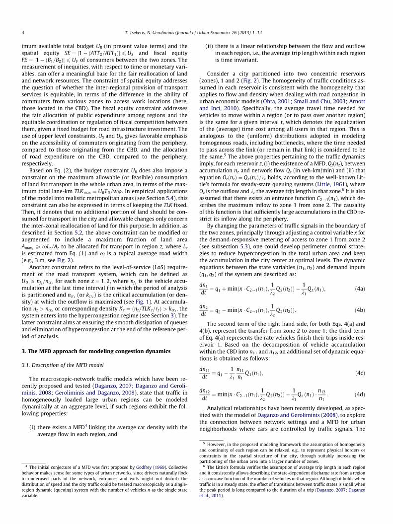
Fig. 2. Concentric city configuration.

T. Tsekeris, N. Geroliminis / Journal of Urban Economics 76 (2013) 1–14 3

sents the MFD approach and compares it with existing models ofcongestion. Section 4 describes simulation experiments for theoptimal allocation of urban land and network resources in thepresence of various constraints. Section 5 extends these experi-ments by allowing all of the available urban parameters to varyand it performs a sensitivity analysis of the results. It also analyzeshow the MFD can be used for the robust design of alternative pol-icies, such as metering of access through perimeter control andoptimal allocation of land for transport, to reduce congestionexternalities. In addition, it shows the results from implementingthe MFD model into major cities with realistically representativesettings. Section 6 summarizes and provides conclusions.

2. Concentric city model

Let us assume a concentric city with two zones: the inner core,z = 1, and the periphery, z = 2. The total area is equal toA ¼

PzAz ¼ A1 þ A2 ¼ pR2

1 þ pðR2 � R21Þ, where the total radius

R = R1 + R2 (see Fig. 2). The city is closed with a total populationP =

PzPz = P1 + P2, and two land uses, only residence at zone 2

and both residence and employment at zone 1. Both the housingand employment locations of each consumer are fixed. By definingthe population density of zone z as Dz = Pz/Az and the density ratiobetween the two zones as rd = D2/D1, then, the population at zone 2can be expressed as a function of the density ratio,2 i.e.,P2 ¼ A2rdD1.

Assuming that each urban zone z is spatially organized insquare blocks of average length Lbz , which is equal to the averageintersection spacing or link length (distance between two consec-utive traffic lights per block, see the inset view of Fig. 2), the totalnumber of blocks can be continuously approximated asNbz ¼ Az=L2

bz. By uniformly partitioning the total area of a region

into a finite number of square block groups, the number of lane-km can be approximated by multiplying the total number of blocksides with the average link length Lbz and the average number ofroad lanes ‘z at that zone, as follows:

Lz ffi 2ðNbz þffiffiffiffiffiffiffiNbz

pÞLbz‘z; ð1Þ

The model sets certain assumptions about the average linklength Lbz and number of lanes ‘z (Section 4), which yield the totalnetwork length, in terms of total lane-km TLK = L1 + L2. By denotingas w the unit price per lane-km, in monetary units (mu/lane-km),

2 Although the population density gradually changes from the CBD to theresidential area in several real cases, the conventional assumption of the concentriczoning system allows the plausible separation of urban space into two zones withdistinct land uses (residential and mixed) and the investigation of various zone-specific urban policies, such as boundary growth control, region-wide changes ofstreet network or block densities, perimeter controls and cordon toll pricing.

the total budget required for road construction and maintenancecosts in zone z is wLz. The present value of this budget can be ob-tained through Eq. (2), where / is a depreciation factor:

Bz ¼wLz/

TD; where / ¼ r0ð1þ r0ÞTD

ð1þ r0ÞTD � 1ð2Þ

This relationship expresses the present value of annuity pay-ments, which refer to a stream of fixed payments over a specifiedperiod of time (annually), taking into account the time value ofmoney, interest rate r0 and duration TD (in years) of the design per-iod of analysis (Lasher, 2008). It is noted that the representation ofcapital depreciation is not constrained by Eq. (2) and other func-tions may well be used for this purpose.

The individual demand is assumed here as perfectly inelasticand there is absence of tolls; hence, there are not components ofconsumer surplus and toll revenues. Thus, the efficiency gainsresulting from an optimal urban plan (in terms of the city size, landuse and network configuration) can be defined by minimizing thedeadweight loss,3 by saving per-capita average time cost or aggre-gate infrastructure capital and time costs, in monetary terms. Thelatter measure expresses the total social cost (for both the govern-ment and consumers). The present value of the total social cost, TSCz,encompasses the infrastructure (budget) cost, Bz, and the total traveltime sz. In order to take into account the population heterogeneity,the transformation of sz into monetary units relies on weightingwith the corresponding value of travel time VOTTz of commuterswhose origin is located at zone z.

Let us decompose the vehicle accumulation within the CBD asn1 = n11 + n12, where n11 and n12 are the numbers of vehicles inzone 1, which originated from zones z = 1 and z = 2, respectively(time index is omitted for brevity), and denote the vehicle accumu-lation in zone 2 as n2. Provided that interval t has duration of oneminute, each vehicle traveling either in zone 1 or zone 2 adds tothe trip cost of the corresponding zone one minute of travel duringthe period T of analysis. By aggregating the intervals in which eachvehicle is traveling in the zones 1 and 2 over the period T, the totaltravel time in each of the zones (expressed in veh-h) is s1 =

RTn11(-

t)dt and s2 ¼R

Tðn2ðtÞ þ n12ðtÞÞdt, respectively. Then, the total socialcost in the whole urban area can be expressed as:

TSC ¼X

z

TSCz ¼X

z

½Bz þ pasz�

¼ ½B1 þ paVOTT1s1� þ ½B2 þ paVOTT2s2�; ð3Þ

where pa refers to a factor projecting the estimated travel time sz forthe period of analysis to the whole peak travel period of a typicalday (weekday) on a yearly basis. By assuming that the trip costsare mostly accumulated in the morning peak period and theremaining period of a typical day accounts for the 50% of the tripcosts of the peak period, and given that the typical days of a yearamount to 260 (by excepting the weekends), it is obtained thatpa = 1.5 ⁄ 260 = 390. As it was explained before, the problem objec-tive can be associated with the minimization of either the TSC or thetotal average per-capita travel time ATT = (s1 + s2)/qP, where q isthe car ownership index (cars/person), assumed to be the samefor both zones. Subsequently, it holds that the per-capita travel timespent by the consumers whose origin is located at zone z = 1, 2 isATTz = sz/(qPz).

The minimization of the above objectives may be subject to so-cial, fiscal, regulatory, operational and physical constraints. Suchconstraints may be related to budget and equity problems typicallyarising in the design of city characteristics. They involve the max-

3 By assuming the lot sizes as fixed, consumers derive variable utility only fromother goods, and with fixed overall resources, those available for other goods aremaximized when aggregate transport costs are minimized.

4 T. Tsekeris, N. Geroliminis / Journal of Urban Economics 76 (2013) 1–14

imum available total budget UB (in present value terms) and thespatial equity SE ¼ j1� ðATT2=ATT1Þj 6 US and fiscal equityFE ¼ j1� ðB1=B2Þj 6 UF of consumers between the two zones. Themeasurement of inequities, with respect to time or monetary vari-ables, can offer a meaningful base for the fair reallocation of landand network resources. The constraint of spatial equity addressesthe question of whether the inter-regional provision of transportservices is equitable, in terms of the difference in the ability ofcommuters from various zones to access work locations (here,those located in the CBD). The fiscal equity constraint addressesthe fair allocation of public expenditure among regions and theequitable coordination or regulation of fiscal competition betweenthem, given a fixed budget for road infrastructure investment. Theuse of upper level constraints, US and UF, gives favorable emphasison the accessibility of commuters originating from the periphery,compared to those originating from the CBD, and the allocationof road expenditure on the CBD, compared to the periphery,respectively.

Based on Eq. (2), the budget constraint UB does also impose aconstraint on the maximum allowable (or feasible) consumptionof land for transport in the whole urban area, in terms of the max-imum total lane-km TLKmax ¼ UBTD=wu. In empirical applicationsof the model into realistic metropolitan areas (see Section 5.4), thisconstraint can also be expressed in terms of keeping the TLK fixed.Then, it denotes that no additional portion of land should be con-sumed for transport in the city and allowable changes only concernthe inter-zonal reallocation of land for this purpose. In addition, asdescribed in Section 5.2, the above constraint can be modified oraugmented to include a maximum fraction of land areaAmaxz P xLz=Az to be allocated for transport in region z, where Lz

is estimated from Eq. (1) and x is a typical average road width(e.g., 3 m, see Fig. 2).

Another constraint refers to the level-of-service (LoS) require-ment of the road transport system, which can be defined asUO P nfz=ncrz for each zone z ¼ 1;2, where nfz is the vehicle accu-mulation at the last time interval f in which the period of analysisis partitioned and ncrz (or kcrz ) is the critical accumulation (or den-sity) at which the outflow is maximized (see Fig. 1). At accumula-tion nz > ncrz or corresponding density Kz ¼ ðnz=TLKz=‘zÞ > kcrz , thesystem enters into the hypercongestion regime (see Section 3). Thelatter constraint aims at ensuring the smooth dissipation of queuesand elimination of hypercongestion at the end of the reference per-iod of analysis.

3. The MFD approach for modeling congestion dynamics

3.1. Description of the MFD model

The macroscopic-network traffic models which have been re-cently proposed and tested (Daganzo, 2007; Daganzo and Geroli-minis, 2008; Geroliminis and Daganzo, 2008), state that traffic inhomogeneously loaded large urban regions can be modeleddynamically at an aggregate level, if such regions exhibit the fol-lowing properties:

(i) there exists a MFD4 linking the average car density with theaverage flow in each region, and

4 The initial conjecture of a MFD was first proposed by Godfrey (1969). Collectivebehavior makes sense for some types of urban networks, since drivers naturally flockto underused parts of the network, entrances and exits might not disturb thedistribution of speed and the city traffic could be treated macroscopically as a single-region dynamic (queuing) system with the number of vehicles n as the single statevariable.

(ii) there is a linear relationship between the flow and outflowin each region, i.e., the average trip length within each regionis time invariant.

Consider a city partitioned into two concentric reservoirs(zones), 1 and 2 (Fig. 2). The homogeneity of traffic conditions as-sumed in each reservoir is consistent with the homogeneity thatapplies to flow and density when dealing with road congestion inurban economic models (Ohta, 2001; Small and Chu, 2003; Arnottand Inci, 2010). Specifically, the average travel time needed forvehicles to move within a region (or to pass over another region)is the same for a given interval t, which denotes the equalizationof the (average) time cost among all users in that region. This isanalogous to the (uniform) distributions adopted in modelinghomogenous roads, including bottlenecks, where the time neededto pass across the link (or remain in that link) is considered to bethe same.5 The above properties pertaining to the traffic dynamicsimply, for each reservoir z, (i) the existence of a MFD, Qz(nz), betweenaccumulation nz and network flow Qz (in veh-km/min) and (ii) thatequation OzðnzÞ ¼ Q zðnzÞ=kz holds, according to the well-known Lit-tle’s formula for steady-state queuing systems (Little, 1961), whereOz is the outflow and kz the average trip length in that zone.6 It is alsoassumed that there exists an entrance function C2?1(n1), which de-scribes the maximum inflow to zone 1 from zone 2. The causalityof this function is that sufficiently large accumulations in the CBD re-strict its inflow along the periphery.

By changing the parameters of traffic signals in the boundary ofthe two zones, principally through adjusting a control variable x forthe demand-responsive metering of access to zone 1 from zone 2(see subsection 5.3), one could develop perimeter control strate-gies to reduce hypercongestion in the total urban area and keepthe accumulation in the city center at optimal levels. The dynamicequations between the state variables (n1, n2) and demand inputs(q1, q2) of the system are described as:

dn1

dt¼ q1 þminðx � C2!1ðn1Þ;

1k2

Q 2ðn2ÞÞ �1k1

Q 1ðn1Þ; ð4aÞ

dn2

dt¼ q2 �minðx � C2!1ðn1Þ;

1k2

Q 2ðn2ÞÞ: ð4bÞ

The second term of the right hand side, for both Eqs. 4(a) and4(b), represent the transfer from zone 2 to zone 1; the third termof Eq. 4(a) represents the rate vehicles finish their trips inside res-ervoir 1. Based on the decomposition of vehicle accumulationwithin the CBD into n11 and n12, an additional set of dynamic equa-tions is obtained as follows:

dn11

dt¼ q1 �

1k1

n11

n1Q 1ðn1Þ; ð4cÞ

dn12

dt¼minðx � C2!1ðn1Þ;

1k2

Q 2ðn2ÞÞ �1k1

Q 1ðn1Þ �n12

n1: ð4dÞ

Analytical relationships have been recently developed, as spec-ified with the model of Daganzo and Geroliminis (2008), to explorethe connection between network settings and a MFD for urbanneighborhoods where cars are controlled by traffic signals. The

5 However, in the proposed modeling framework the assumption of homogeneityand continuity of each region can be relaxed, e.g., to represent physical borders orconstraints in the spatial structure of the city, through suitably increasing thepartitioning of the urban area into a larger number of zones.

6 The Little’s formula verifies the assumption of average trip length in each regionand it consistently allows describing the state-dependent discharge rate from a regionas a concave function of the number of vehicles in that region. Although it holds whentraffic is in a steady state, the effect of transitions between traffic states is small whenthe peak period is long compared to the duration of a trip (Daganzo, 2007; Daganzoet al., 2011).

Fig. 3. Trapezoidal shape of travel demand profile (distribution of departure times)for the concentric city.

Fig. 4. Relationship between travel demand and cost under different demandprofiles for the concentric city.

7 This traditional network supply curve was first introduced by Pigou (1920) andapplied in most marginal-cost pricing models.

T. Tsekeris, N. Geroliminis / Journal of Urban Economics 76 (2013) 1–14 5

MFD for each region, Qz(nz), can be expressed as a function of: (i)network variables: average link length, Lbz , and average numberof lanes, ‘z; (ii) link variables for one lane (common for both re-gions): free-flow speed, uff, jam density of a fully congested road,kj, saturation flow, s (maximum flow of cars during green time),and congested wave speed (speed of queue length increase whenvehicles at saturation flow approach a red light and stop),uw ¼ uff =ðkjuff =s� 1Þ; and (iii) intersection variables: signal cycleoffset, d (the time difference at the beginning of green betweenadjacent traffic signals), cycle time, C, and green time, G. The scala-bility of flows from a series of links to large traffic networks is not astraightforward transformation. Route or network capacity can besignificantly smaller than the sum of capacities of constituent sin-gle links, because of the correlations developed through the differ-ent values of offsets. The offsets affect network capacityconsiderably when blocks are short.

In the MFD, any set of flow Qz (or outflow Oz) and accumulationnz (or network traffic density Kz) values relates to some level of(hyper)congestion, which depends on the network traffic capacityof region z. The capacity refers to the maximum flow Q maxZ

in theregion, at the critical accumulation ncrz (or critical density kcrz ),and it depends on the zone width Rz and the average intersectionspacing (link length) Lbz and number of lanes ‘z. Based on the dy-namic traffic loading of the two regions according to the demandprofile shown in Fig. 3 and following Eqs. 4(a)–4(d), the non-mono-tonic pattern of the MFD for region z is derived by fitting two dis-tinct second-degree polynomials of the form Q z ¼ a1n2

z þ a2nz þ a3.The set of parameters (a1;a2;a3) corresponds to a specific linklength Lbz and is calibrated separately for the upward (congested)and downward (hypercongested) parts of the curve (Fig. 1). Theoptimal plan resulting from this pattern relates the flow Qz(nz),for a given vehicle accumulation nz and traffic density Kz in the re-gion, to a given land use density (or block density, in terms of thenumber of blocks with a specific land use per unit area). The MFDmodel can ensure the maximum flow and throughput in the casewhere critical density is reached, beyond which the network be-comes hypercongested and the flow decreases.

Through the MFD pattern, the diseconomies of scale and densityin each region are taken into account. Hence, in contrast with thetraditional economic models, the present one can plausibly explainhow congestion costs (diseconomies of agglomeration) in the citywill force changes in the optimal amount of land and network re-sources, or their reallocation from one region to another. In thisway, the MFD allows directly the use of flow and car density astwo policy instruments which affect the city size, land use andblock density, and network structure.

Fig. 1 shows an example of a MFD specified for the concentriccity model (Fig. 2), with total area A = 120 km2 and equal zonewidths R1 ¼ R2 ¼ 3:09 km. The network variables are defined as

Lb1 = Lb2 = 100 m (meters), ‘1 = 2.0 and ‘2 = 1.5, while the valuesof link and intersection variables are the same to those used in Sec-tion 4. In this section, we assume that the demand profile for bothzones has a symmetrical trapezoidal shape, with a total morningperiod of analysis equal to 360 min (minutes) and a peak periodlength of 120 min, and zonal populations P1 = 1.076 andP2 = 1.872 million residents (with car ownership index q = 0.5).These values make the system exhibit hypercongestion. The mag-nitude of demand input in each zone is determined in analogy withthe regional allocation of population (Fig. 3).

3.2. Comparison with existing models

Consider the dynamical system of a two-region city (Section 2)governed by Eqs. 4(a)–4(d). Simulations run with different demandsizes (total trips per day) and lengths of peak period, i.e., 1 h (high-est peak), 2 h, 3 h and 6 h (flat demand). The system returns touncongested conditions by the end of simulation period, i.e., thesame number of trips is completed for runs having the same de-mand size. The results are summarized in Fig. 4. It is clear thatwhen traffic conditions are undersaturated and demand is low,the effect of variation in demand (as expressed with the peak per-iod length) is negligible. The reason is that the MFD has almost lin-ear behavior for small values of accumulation (see Fig. 1) and thetotal delay is not sensitive to small variations of flow within the gi-ven period. But, once the dynamical system of the two-region cityenters the congested regime of the MFD for one of the regions, thenassuming an average cost-demand curve creates significant errors.As expected, the more concentrated peak periods (and, hence,higher peak-period accumulations) are associated with higher in-crease of travel cost in relation to demand size, compared to themore dispersed and flat peak periods.

Fig. 5 illustrates the differences in the results obtained from theuse of the MFD and a simple, static model (SM) of network trafficcongestion. The SM adopts a simple supply function, where traveltime at every instance is an increasing function of the inflow.7 Inthe SM, the travel cost conditions are stationary and the networktraffic inflow solely depends on the given (trapezoidal with a 2 h-peak period) pattern of demand and traffic capacity constraints,based on the specific city configuration. Namely, it ignores the net-work traffic dynamics, as described in the Eqs. 4(a)–4(d), which takeinto account time-varying changes of trip flows and travel costresulting from previous time intervals due to queuing (in consis-tency with the physics of hypercongestion), and uncompleted trips,which is a function of the network outflow.

(a) (b)

(c) (d)

Fig. 5. Comparison of results obtained from the MFD and a static model (SM) of network traffic congestion based on supply functions for different population sizes (inmillion) for (a) region 1 and (b) region 2, and estimating (c) the day period-average travel time per vehicle trip for different population sizes, and (d) the per-vehicle averagetravel time for each time interval (when P = 1.7 million).

6 T. Tsekeris, N. Geroliminis / Journal of Urban Economics 76 (2013) 1–14

The MFD model supply function is dynamically specified byplotting the per-vehicle average travel time for each interval t forthe inner region 1 (Fig. 5a) and outer region 2 (Fig. 5b), TT1(t)and TT2(t), as a function of the demand input of each region, q1(t)and q2(t), respectively. The different scenarios are analyzed forpopulation sizes ranging from P = 1.3 million to P = 1.9 million.The supply function of the SM is correspondingly determined foreach region and population size by calibrating a best-fit curve torepresent the static relationship between travel time and inflowdemand for each interval t (Fig. 5a and b). In contrast with theSM, the supply curves of the MFD model form loops. These loopssignify that transport networks are not memory-less, since thesame inflow will create higher travel times in a more congestedstate, compared to an initially less congested (or uncongested)state. They also show that vehicles at the offset of hypercongestionexperience higher travel times for the same inflow than at the on-set of hypercongestion. In region 2 (Fig. 5b), for population P < 1.6million, there is no significant congestion and all curves producedby the MFD model are similar. For both regions and smaller popu-lation sizes, the initial segments of the curves formed by the SMand the MFD tend to coincide at the uncongested part. The errorresulting from the SM is magnified with the increase of congestionand growth of population (for P P 1:6 million).

Fig. 5c summarizes the comparison of the results of the SM andMFD for the day period-average travel time per vehicle trip, TTSM

and TTMFD, respectively, for increasing population (every P = 0.03million) between P = 1.3 million and P = 1.9 million. It is found thatthe results of the two models are the same (TTSM ¼ TTMFD) when

P = 1.7 million (at point A), the SM overestimates (TTSM > TTMFD)the day period-average travel cost when P < 1.7 million and under-estimates it (TTSM < TTMFD) when P > 1.7 million. However, as it isshown in Fig. 5d, even when TTSM ¼ TTMFD, the SM is not able toaccurately estimate the trip cost in the urban area. This is becausethe per-vehicle average travel time TTSM(t) resulting from the SMmay present significant intra-day deviations (depending on thetime-of-day traffic conditions) from the per-vehicle average traveltime TTMFD(t) resulting from the MFD. Specifically, when P = 1.7million, the overestimation and underestimation errors of theSM, in relation to the MFD, are equalized and canceled out overthe day period (Fig. 5d). The inaccurate modeling of the flow-den-sity relationship and congestion costs through the SM may lead tomisallocation of land and network resources in the urban area, andit cannot be utilized for deploying intra-day dynamic traffic man-agement schemes, such as perimeter control and congestionpricing.

4. Model application with both fixed and variable parameters

In the current simulations, the two-region city has a total basepopulation P = 1.3 million, fixed density ratio rd = 0.5 (i.e., the pop-ulation density in the periphery is half that of the CBD) and carownership index q = 0.5. The urban topology characteristics are de-scribed by six parameters: the average block (or link) lengths, Lb1

and Lb2, and average number of lanes, ‘1 and ‘2, in zones 1 and 2,respectively, zone width ratio R2/R1, which produces R1 and R2

(for the case of fixed R), and zone width R2, which produces R2/R1

T. Tsekeris, N. Geroliminis / Journal of Urban Economics 76 (2013) 1–14 7

ratio (for the case of variable R2). In all the experiments, the per-missible values of average link length are ranging from 70 to500 m and of average number of lanes from 1 to 3, for both zones.

Each combination of optimized parameter values results in adifferent plan, with respect to the city size, land use and networkconfiguration, whose efficiency is evaluated with either the totalsocial cost, TSC, or the average per-capita travel time, ATT. In orderto create some intuition about how topological parameters affectthe different objectives, some preliminary analysis is performedfirst, wherein only two parameters (out of the six) are optimizedconsidering the others as fixed. This situation could be due toimposition of physical, administrative or other constraints to theplanning process. More specifically, the first set of experiments(plans 1–4) assumes that the total radius is fixed R = 6.18 km,hence, the total urban area is A = 120 km2. The second set of exper-iments (plans 5–6) relaxes the above restriction and assumes afixed CBD radius R1 = 3 km and variable size of the outer zone witha minimum width R2 = 3 km. The optimized parameters are as fol-lows: Lb1 and Lb2 for plan 1, R2/R1 and Lb2 for plan 2, R2/R1 and ‘2 forplan 3, Lb2 and ‘2 for plan 4, R2 and Lb2 for plan 5, and R2 and ‘2 forplan 6. Later, in Section 5, a full optimization framework is demon-strated that allows identifying optimal solutions for all availableparameters.

The critical values of the model parameters have been experi-mentally evaluated in previous simulated and real case studies(Geroliminis and Daganzo, 2008). They are assumed to be propor-tional to the size of reservoirs: free-flow speed uff = 43.25 km/h,jam density kj = 0.14 veh/m, saturation flow s = 1700 cars per hourper lane during green time, traffic signal cycle length C = 90 s,green time G = 40.5 s and a satisfactory signal offset to provide effi-cient coordination between traffic signals. It is assumed that theaverage trip lengths in zones 1 and 2 are k1 ¼ 1:2R1 andk2 ¼ 0:8R2. The average value of travel time for commuters inzones 1 and 2 are VOTT1 = 10 mu/hour and VOTT2 = 6 mu/hour.The temporal profile of demand is assumed to follow a trapezoidalshape (Fig. 3), with total period of analysis equal to 360 time inter-vals and (morning) peak period equal to 120 intervals. In terms ofthe infrastructure cost parameters (see Eq. (2)), the unit pricew = 15 million mu/lane-km, the interest rate r0 = 0.1 and the designperiod of analysis TD = 15 years.

Let us define nmax as the maximum vehicle accumulation in theanalysis period. Based on suitably scaling the total base population,three scenarios about the levels of demand and resulting conges-tion conditions for both zones are defined as follows:

(a) reduced demand, which refers to low or mild congestionwith 0:5 6 nmax=ncr < 0:9 during the peak period,

(b) moderate demand, which refers to system operation inclose-to-capacity conditions, such that 0:9 6 nmax=ncr < 1:0during the peak period, and

(c) increased demand, which refers to system operation in over-saturated conditions (hypercongestion), such thatnmax=ncr P 1:0 during the peak period.

Table 1Optimal values of parameters for minimization of TSC and ATT (in parenthesis) objective f

Note: Bold values in the white cells indicate the optimized parameters, non-bold valparameters and the shadowed cells include input values in each scenario. The same not

In each scenario, these changes yield a different optimal set ofparameters and selected urban plans. In the plans 1–4, whereinthe population density is kept fixed for the total urban area, onlyinter-zonal changes in density are allowed. In the plans 5–6, thepopulation density is only influenced by changes in the optimalland provision in the periphery. Tables 1–6 summarize the resultsfor different levels of congestion (low, close-to-capacity, hypercon-gestion) conditions, by showing the values of network parameters(average block length and lane number), zone widths, TSC and ATT,spatial and fiscal equity, and total required budget (in billion mu orbmu).

In all the cases considered, the increase of demand level andcongestion conditions, from reduced demand (Tables 1 and 2) tomoderate demand (Tables 3 and 4) and, then, increased demand(Tables 5 and 6), leads to increased TSC and ATT, as well as largerinvestment needs, since the number of commuters who must beserved also increases. The higher budget is invested to create moredense networks to keep the service quality for the increased de-mand at an acceptable level. For instance, in plan 1, when minimiz-ing the TSC, block lengths decrease (and budget increases) as thedemand moves from low to moderate conditions, i.e., fromLb1 ¼ 140 m and Lb2 ¼ 480 m (B = 0.193 bmu) to Lb1 = 130 m andLb2 = 310 m (B = 0.279 bmu) (plan 1a), respectively, and then tohypercongestion conditions, to Lb1 = 120 m and Lb2 = 220 m(B = 0.360 bmu).

In Tables 3 and 4, plans 1a and 1b are comparatively examinedto evaluate the impact of different CBD boundary constraints, interms of setting the value of R2/R1 ratio equal to 1.00 and 0.50,respectively, on various performance measures. The increase ofland occupied by the CBD, relative to the periphery (plan 1b), leadsto the reduction of TSC and, particularly, of ATT, and the increase oftotal budget. Similarly, the results of plans 2 and 3, where the totalradius R is held fixed, demonstrate that reducing the R2/R1 ratio,which implies increasing the share of commuting within theCBD, as traffic congestion increases, leads to diminishing the TSCand ATT.

The current findings are important because they take into ac-count the exact fraction of land that is assigned to each use (resi-dential and mixed), in contrast with the traditional urbaneconomic analysis, where land use patterns typically refer to exclu-sive zones or rings for each use. Hence, they can provide useful in-sight into the optimal share of land use mixing in the urban area,even in hypercongestion conditions. The results verify previousfindings in the relevant economic literature that fully interspersed(residential and employment) land use is never optimal (consider-ing congestion effects) and that mixing in the CBD becomes opti-mal when traffic demand equilibrates at some level of congestion(Wheaton, 2004). The results are also consistent with those ofMcDonald (2009), in which the selective movement of householdswith commuters from an outer ring to an inner ring where theywork was found to reduce congestion costs and improve efficiencyin a monocentric city.

unctions under the reduced demand scenario.

ues in the white cells indicate dependent variables obtained from the optimizedation is used in Tables 3 and 5.

Table 2Results of simulation analysis for different planning objectives and policy plans under the reduced demand scenario.

Variable Objective Plan 1 Plan 2 Plan 3 Plan 4 Plan 5 Plan 6

TSC (bmu) TSC min 0.403 0.377 0.447 0.425 0.419 0.428ATT min 0.478 0.425 0.505 0.497 0.459 0.538

ATT (min) TSC min 7.144 6.721 7.818 6.864 6.335 6.761ATT min 6.501 6.357 7.070 6.232 6.236 6.137

Budget (bmu) TSC min 0.193 0.187 0.235 0.224 0.232 0.230ATT min 0.287 0.246 0.312 0.312 0.274 0.356

Spatial equity TSC min 1.108 1.263 1.287 1.188 1.021 1.191ATT min 1.036 1.095 1.041 0.924 0.979 0.927

Fiscal equity TSC min 0.487 0.194 0.296 0.894 0.467 0.937ATT min 0.043 0.290 0.259 0.115 0.014 0.258

Table 3Optimal values of parameters for minimization of TSC and ATT (in parenthesis) objective functions under the moderate demand scenario.

Table 4Results of simulation analysis for different planning objectives and policy plans under the moderate demand scenario.

Variable Objective Plan 1a Plan 1b Plan 2 Plan 3 Plan 4 Plan 5 Plan 6

TSC (bmu) TSC min 0.822 0.802 0.731 0.832 1.043 0.599 0.641ATT min 0.963 0.906 0.920 0.960 1.118 0.671 0.766

ATT (min) TSC min 11.514 8.181 8.430 8.454 15.640 7.533 8.154ATT min 11.096 7.718 7.710 7.868 15.216 7.153 7.520

Budget (bmu) TSC min 0.279 0.360 0.311 0.375 0.280 0.260 0.266ATT min 0.437 0.490 0.498 0.495 0.377 0.333 0.416

Spatial equity TSC min 1.845 0.851 0.983 0.898 2.826 1.078 0.962ATT min 1.711 0.857 0.851 0.842 2.699 0.883 0.741

Fiscal equity TSC min 0.359 0.936 0.521 0.262 0.316 0.391 0.321ATT min 0.420 0.384 0.567 0.927 0.257 0.166 0.428

Table 5Optimal values of parameters for minimization of TSC and ATT (in parenthesis) objective functions under the increased demand scenario.

Table 6Results of simulation analysis for different planning objectives and policy plans under the increased demand scenario.

Variable Objective Plan 1 Plan 2 Plan 3 Plan 4 Plan 5 Plan 6

TSC (bmu) TSC min 0.861 0.797 0.894 1.481 0.883 0.886ATT min 0.942 0.956 0.998 1.538 1.045 1.001

ATT (min) TSC min 8.712 8.665 8.619 18.093 12.972 13.025ATT min 7.891 7.868 8.035 17.765 12.473 12.235

Budget (bmu) TSC min 0.360 0.331 0.391 0.420 0.264 0.265ATT min 0.490 0.498 0.495 0.494 0.442 0.407

Spatial equity TSC min 0.805 0.974 0.887 2.488 1.851 1.865ATT min 0.840 0.837 0.828 2.409 1.545 1.481

Fiscal equity TSC min 0.936 0.722 0.510 0.606 0.346 0.338ATT min 0.384 0.567 0.927 0.101 0.478 0.408

8 T. Tsekeris, N. Geroliminis / Journal of Urban Economics 76 (2013) 1–14

T. Tsekeris, N. Geroliminis / Journal of Urban Economics 76 (2013) 1–14 9

This outcome concerning the land use mixing (or share of com-muting) in the CBD can be attributed to the decrease of trip delaysdue to the reduced total distance traveled. This is because of theincreasing share of intra-zonal trips, compared to the inter-zonaltrips, as the width ratio R2/R1 decreases. Besides, the reduction ofthe ATT (plan 1a vs. plan 1b) and R2/R1 ratio, as the congestion levelincreases, result in improvement (toward zero) of the spatial equi-ty metric, while the impact on fiscal equity is reversed. Therefore,in the presence of urban boundary constraints, the growing levelsof congestion favor more compact city development, through mix-ing land uses in the inner area, to reduce delay externalities andimprove spatial equity. The requirements (set as UO1;2 ¼ 0:50, forthe level-of-service, US = 2.0, for spatial equity, and UF = 1.0, for fis-cal equity) are found to be ensured (not binding) in all cases, ex-cept for plan 4 in the moderate and increased demand scenarios(Tables 4 and 6, respectively), where SE > 2.0. In the latter case,the spatial equity constraint must be relaxed to yield a feasibleoptimal plan.

At all levels of traffic congestion, plan 2 (in the first set of exper-iments) and plan 5 (in the second set of experiments) are found toproduce the lowest TSC and ATT. Namely, the average block length(or link length) in zone 2 can provide the best possible designinstrument to mitigate congestion externalities, in conjunctionwith changing either the share of urban land in favor of the CBDor the total urban boundary for a fixed CBD area. Specifically, in-crease of the outer area block density, i.e., a shorter average linklength Lb2 (improvement of the street network connectivity in zone2), as well as increase of the CBD area, entails improvement of thesystem capacity. This is because of the increase of the density of ac-cess roads and throughput, i.e., the rate vehicles enter into the CBD.On the other hand, increase of the average block density entails alarger total number of links and, hence, a higher amount of roadinvestment (construction and maintenance cost).

5. An optimization framework for parameter estimation

5.1. Unconstrained optimization results

In this subsection, the TSC and ATT are minimized with respectto all available parameters without imposing constraints. The leastpossible assumptions are made to ensure a plausibly allowable sizeof road infrastructure (see Section 4) and distinct separation be-

Table 7Optimization results with respect to TSC and ATT for different population size and urban g

Objective Variable Population in millions (with fixed R)

1.3 1.95 2.6

TSC minimization TSC (bmu) 0.382 0.656 0.852ATT (min) 5.749 7.736 7.811Lb1 0.070 0.103 0.070Lb2 0.496 0.274 0.358‘1 2.290 2.007 2.075‘2 2.071 1.414 2.366R2/R1 2.203 1.832 1.101Budget 0.227 0.304 0.382Spatial equity 1.239 0.995 0.930Fiscal equity 0.176 0.582 0.283

ATT minimization TSC (bmu) 0.524 0.762 1.035ATT (min) 5.827 6.475 7.067Lbl 0.097 0.070 0.070Lb2 0.292 0.258 0.206‘1 2.949 2.731 2.909‘2 2.130 2.584 2.643R2/R1 1.449 1.384 1.096Budget 0.361 0.587 0.621Spatial equity 1.156 1.023 0.971Fiscal equity 0.170 0.177 0.052

tween the two urban zones, to facilitate understanding of the mod-el and interpretation of the results. The plans are investigated fordifferent levels of demand, by gradually (using a factor of 1.5)increasing the total population size, i.e., P = 1.30, 1.95, 2.60 and3.25 million. The unit prices and parameter values of infrastructurecosts and the lengths of the total and peak period are the same tothose adopted in Section 4. The optimization process is based onmultiple runs of a steepest descent (SD) search routine to avoid lo-cal optima. It is known that the traditional SD method can betrapped to local minima. To address this weakness, the SD ap-proach is combined with an initial random search in each consec-utive run to identify a set of good initial solutions and improve the‘best’ solution of the previous run. Table 7 presents the optimal val-ues for the TSC and ATT, and the estimated parameter values andmeasures of equity and budget (which do not express constraintsbut they are outcomes of the optimization process), for differentpopulation size and urban growth scenarios.

The optimization results, which involve a higher degree of free-dom, are found to be consistent with those described in the previ-ous section. Specifically, larger population sizes are associated withhigher expenditure and delay externalities, as reflect the increasedvalues of the TSC and ATT. In addition, they suggest a more compactpattern of urban development, as implied by the shorter averageblock length, particularly for zone 2 (Lb2), and the smaller ratioR2/R1, for both urban boundary growth scenarios (i.e., with fixedR and fixed R1). The reduction of commuting share from zone 2,compared to the CBD, decreases the average travel time ATT2 ofvehicles originating from that zone, in relation to the ATT1, thusimproving (moving closer to zero) the measure of spatial equity(based on ATT minimization). On the other hand, the measure offiscal equity deteriorates (moves away from zero). This is becausethe CBD attracts more investments as it increasingly consumesmore of the available land, relative to the periphery. The next sub-section presents a sensitivity analysis of various parameter valuesand constraints.

5.2. Sensitivity analysis

The rapid growth of large metropolitan areas worldwide setsforth the need for a sensitivity analysis of initial plans on whichthe urban development process has been based. Given the optimalplan settings obtained for different population sizes (Table 7), the

rowth scenarios.

Population in millions (with variable R2)

3.25 1.3 1.95 2.6 3.25

1.172 0.360 0.531 0.705 0.9128.020 6.412 6.356 6.419 6.5700.070 0.175 0.127 0.098 0.0700.263 0.442 0.368 0.341 0.1412.724 2.332 2.719 2.849 2.4352.580 1.677 2.026 2.675 1.6780.880 2.111 1.736 1.060 1.0010.580 0.159 0.228 0.272 0.3330.907 0.929 1.162 1.434 0.8050.540 0.797 1.531 3.233 2.695

1.266 0.481 0.594 0.869 1.0437.738 5.596 6.061 6.247 6.4470.070 0.117 0.095 0.076 0.0700.118 0.368 0.313 0.186 0.1822.971 2.551 2.686 2.831 3.0001.539 2.829 2.032 2.676 3.0000.882 2.561 2.131 1.960 1.8260.682 0.311 0.341 0.472 0.5230.966 0.956 0.982 0.866 0.8260.279 0.140 1.207 0.480 0.614

(a) (b)

(c) (d)

Fig. 6. Sensitivity analysis of the ATT with respect to percentage increase in demand for the cases of fixed total radius under (a) minimizing the ATT and (b) minimizing theTSC, and fixed CBD radius under (c) minimizing the ATT and (d) minimizing the TSC.

10 T. Tsekeris, N. Geroliminis / Journal of Urban Economics 76 (2013) 1–14

TSC and ATT are re-estimated for increasing (%) rates of travel de-mand growth. As it is shown in Fig. 6a–d, the optimal plans corre-sponding to smaller population sizes (1.3 and 1.95 million) yieldhigher ATT as the demand growth rate increases, compared tothose corresponding to larger population sizes (2.6 and 3.25 mil-lion), for both minimization problems and boundary growthscenarios.

Specifically on the basis of the ATT minimization, when R isfixed (see Fig. 6a), the ATT remains small up to a 25% increase indemand, but then it remarkably increases from 5.8 min to42 min, for initial population size of 1.3 million, and from6.5 min to 26 min, for initial population size of 1.95 million, whenthe level of demand increases by 70%. Values of ATT more than30 min indicate that the system is unable to return to uncongestedconditions by the end of the period. However, the ATT increasesonly from 7.1 min to 22 min, for initial population size of 2.6 mil-lion, and from 7.7 min to 18 min, for initial population size of 3.25million, for the maximum level of demand increase. These differ-ences can be attributed to the higher total budget and, hence, in-creased road capacity allocated for cases of larger initialpopulation size (see Table 7).

In the case where R is fixed (Fig. 6a), the ATT increases muchsharper with the growth of population, compared to the casewhere only R1 is fixed (Fig. 6c). For instance, for initial population1.30 million, the city becomes highly congested (ATT > 13 min)when population grows by about 30% in the former case, while thisoccurs when population grows by about 70% in the latter case.Therefore, the increase of ATT is getting smaller when planningthe city for higher (possibly expected in the future) populationsizes and when only R1 is kept fixed (R2 is variable). These non-lin-ear changes of ATT with respect to population growth can be inter-preted by the non-monotonic flow-density relationship thatreflects the resulting MFD pattern for each region. The MFD ac-counts for the sensitivity to initial conditions and plausibly ex-plains the diseconomies of a sprawled periphery in relation tothe CBD, compared to traditional economic models of urban con-gestion (see Section 1).

Specifically, this outcome can be attributed to the fact that con-sidering (or predicting) a more crowded urban area, keeping theboundary of the CBD fixed and controlling (compressing) the widthof the residential area, leads to a larger increase of block (or streetnetwork) density. This pattern entails a more compact city devel-opment and higher share of within-CBD commuting, comparedto considering a less crowded urban area and keeping the total ur-ban boundary fixed. Although it induces higher expenditure, theincreased network density results in a MFD shape that is associatedwith less hypercongestion and an enhanced system capacity andthroughput of the residential area. Also, it allows drivers to moreeasily divert to alternative paths (reroute) towards their destina-tion at the CBD and, hence, avoid or experience less congestion de-lays. Such a plan can offer a more robust and sustainable urbandevelopment, particularly in the presence of rapid populationgrowth.

Next, the optimization of ATT is investigated for different popu-lation sizes and available levels of budget, in terms of the fractionof the CBD land area devoted to roads (to enhance the physicalintuition of the results), given the zonal widths. This fraction is as-sumed to be fixed for the periphery and equal to 1/4 of the corre-sponding value for the CBD area. The average road width in bothzones is set equal to x = 3 m. Population size reflects the densityof car trips generated per km2 per day. The results are summarizedas a contour plot in Fig. 7. The plot is divided into six regions: eachregion represents a distinct level-of-service of the auto mobility inthe CBD and the suburban area, as denoted by the ratio n�z ¼ nz=ncrz

of the current accumulation to the critical accumulation (whenn�z > 1, then hypercongestion occurs).

The data points of the plot in region A denote free-flow condi-tions (ATT < 6 min) for the whole duration of the period, while datapoints in region F denote cases where regions reach gridlock(ATT > 30 min), at the value of jam density where vehicles stopmoving. The evolution of n�z over time in the CBD and suburbanarea is graphically illustrated in Fig. 7 for several cases. Plannersshould arguably decide to design the urban network to operatein regions B, C or D. Region A mostly entails a huge infrastructure

Fig. 7. Contour plot of ATT for different values of density of car trip generation (in trips per km2 per day) and fractions of CBD area devoted to roads (this fraction is 4 timessmaller for the suburban area in all cases).

T. Tsekeris, N. Geroliminis / Journal of Urban Economics 76 (2013) 1–14 11

investment cost, as reflects the high portion of CBD land devoted toroads, while regions E and F experience large reductions of the le-vel-of-service, namely, hypercongestion conditions (n�z > 1) for aconsiderable length of the peak period.

Furthermore, the contour plot shows that there are some areasin the upward-moving part of the regions B, C, D and E where asmall increase in the car trip density can significantly increasethe level of congestion and reduce level-of-service. These non-lin-ear changes are observed for the smaller fractions, up to about 15%.Hypercongestion arises in region C (for the suburban area) and re-gions D, E and F (for both the CBD and suburban area), when timeapproaches the mid of the peak period (after t = 200 time units).Thus, the allocation of land (for residence, employment and trans-port) per unit area and the intra-day evolution of congestiondynamics play an important role on how the vehicle accumulationdegrades throughput, given the city size and network operatingcharacteristics. These findings suggest that cities would likely se-lect to trade investment cost for increased levels of robustness innetwork operating conditions, away from those areas where thecost impact of small fluctuations in demand or capacity cannotbe predicted (e.g. due to special events, accidents, etc.). In thisway, planners can make decisions on what percentage of car tripsshould be shifted to public transport to avoid excessive system de-lays. In all the results presented in Fig. 7, an advanced control oftraffic signals has been applied, as it will be described in the nextsubsection.

5.3. The effect of perimeter control

In the case of highly congested networks (for instance, due tohigh population growth relative to network capacity, as shown inFig. 6), the solution of increasing the urban block (or network) den-sity (Section 5.2) can be impractical due to severe fiscal, land avail-ability and other constraints. The deployment of improved trafficcontrol strategies may have an effect similar to that of buildingmore capacity, since it allows more vehicles to use the systemwithin a given period (Button, 2010). An advanced, real-time

perimeter control strategy is required to prevent overcrowding inthe CBD, through the demand-responsive metering of access tomaintain the auto mobility at a stabilized level. For instance, longerred times can be applied into the traffic signal settings across theperimeter of the CBD area during peak hours for phases which di-rect vehicles to the center.

By employing the MFD approach, a simple way to deploy thisstrategy is to monitor the system so that, when traffic densitypasses its critical value, to restrict entry flow from the suburbanarea to the CBD. In this way, the oversaturated traffic flow is con-verted into queues and hypercongestion is eliminated by the end ofthe peak period. In the case where both regions of the city arehighly congested, a more complex strategy should be developed.This control strategy is formulated as an optimization problem,where optimal control values x(t) are identified to minimize theATT, as follows:

minxðtÞATT ¼Z

Tðn1ðtÞ þ n2ðtÞÞdt

� �=qP

subject toDynamic equations 4(a)–4(d)

0 6 xðtÞ 6 1:5; 8t

0 6 n1ðtÞ;n2ðtÞ; 8tð5Þ

The above problem is solved by using the generalized reducedgradient algorithm, which is a well-known, efficient and robustmethodology for solving non-linear programs of general structure.For demonstration purposes, the outcome of Fig. 6b is comparedwith the ATT yielded after implementing the perimeter control,for different population sizes. The results are summarized inFig. 8 for initial population 1.3 million and the same network set-tings. The plots show the evolution of the number of vehicles ineach of the two regions (CBD and suburban area) over time andthe value of parameter x(t), for three population sizes (1.65, 1.85and 1.95 million), with and without perimeter control.

While the perimeter control only slightly improves the ATT forsmaller population sizes, the benefits are found to become signifi-

Fig. 8. Results of ATT as a function of population growth for a given network structure with and without perimeter control between the CBD and the suburban area.

12 T. Tsekeris, N. Geroliminis / Journal of Urban Economics 76 (2013) 1–14

cantly larger for higher population sizes. Note that the system doesnot reach gridlock even for 50% population growth (1.95 million)once the perimeter control is applied, while increased congestionis present for a much smaller population growth (1.65 million)without control (i.e., xðtÞ ¼ 18t). In the case of perimeter control,hypercongestion occurs in the suburban area only for populationof 1.85 and 1.95 million, and n�z always returns to the uncongestedstate at the end of the period. On the contrary, hypercongestion al-ways occurs in the suburban area without control, while n�2 takesvery large values for t > 200 time units and it never returns tothe uncongested state for populations of 1.85 and 1.95 million.

These results indicate that a better utilization of existing roadcapacity through installing an advanced traffic signal control soft-ware can provide an efficient and relatively low-cost policy optionto serve the growing amount of car trips and retain the auto mobil-ity within the city center at a desired level. This option is preferablethan the costly and usually impractical solution of increasing net-work density. Such a policy may be regarded as a desirable alterna-tive (no-toll) second-best optimal strategy compared to the first-best optimum network capacity provision with marginal-cost pric-ing. This particularly holds in cases where dynamic congestioncharging is infeasible due to very expensive (high-technology)investment, increased administrative costs for operating the sys-tem and limited enforcement capacities. Other dynamic trafficmanagement schemes such as time-varying parking fees could alsobe adopted to enhance time cost reductions. Finally, in the case ofhigh demand increase, more sustainable, multi-modal provisionstrategies may be necessary, in order to shift consumers to othermodes, such as bus and metro (out of the road network). The latterissue is outside the scope of this paper, but it definitely constitutesan important research priority.

5.4. Results for typical settings of major cities

The previous findings showed that relatively small changes inthe network capacity (either due to provision or technologyenhancement) can result in significant reduction in trip costs. Inthe present subsection, this is demonstrated by employing typical

settings for large metropolitan areas worldwide, including London,Johannesburg, Mexico City, New Delhi and Mumbai. For the givenpopulation, car ownership index, value of time (based on incomedata from the World Bank), spatial characteristics (R1, A1 andR2, A2) and total available budget (as calculated in terms of theTLK) of these urban areas, optimal plans are estimated with respectto changing network design parameters. Other parameters, such asthose referring to link and intersection variables, and infrastruc-ture costs, are assumed to be the same (as defined in previous sub-sections) for comparison purposes. In order to represent each cityaccording to the simplified concentric urban model (Section 2), auniform block structure is assumed, without regarding the com-plexity associated with the hierarchy of road network.

Each city is simulated as having two concentric zones, i.e., theinner (CBD) area (zone 1) and the outer (residential) area (zone2). For all the cities, the total period of analysis is set equal to360 time intervals (6 h), with a peak period of 240 intervals(4 h). Based on equation (1), the total lane-km of each city can beexpressed as:

TLK ¼ L1 þ L2 ¼ 2ðNb1 þffiffiffiffiffiffiffiffiNb1

pÞLb1‘1 þ 2ðNb2 þ

ffiffiffiffiffiffiffiffiNb2

pÞLb2‘2; ð6Þ

By assuming (e.g., based on map observations) the average blocklength of zone 2, Lb2, the average lane number of zone 2, ‘2, andthe relationship between ‘1 and ‘2 (k ¼ ‘1=‘2) as given, then, forfixed TLK (budget constraint), a number of optimal plans can be ob-tained for different values of ‘1. The average block length of zone 1,Lb1, can be easily estimated, based on Eq. (6), as follows:

Lb1 ¼2kA1‘2Lb2

TLKLb2 � 2kffiffiffiffiffiffiA1p

‘2Lb2 � 2A2‘2 � 2ffiffiffiffiffiffiA2p

‘2Lb2ð7Þ

Table 8 presents the results of optimal plans for the settingscorresponding to each city. In addition to the performance mea-sures used in the previous subsections, the measure of congestionindex is also calculated here. This index is obtained from the ratios/sff of the estimated total travel time (s = s1 + s2) for the wholeperiod to the corresponding total travel time sff at free-flow condi-tions (where nmax=ncr 6 0:1). Moreover, the level of congestion in-dex depicts the magnitude at which the trip cost is underestimated

Table 8Results of optimization plans for typical settings corresponding to major cities for different k ¼ ‘1=‘2 values. Source for population and geographical data: www.urban-age.net.

London Johannesburg Mexico City New Delhi Mumbai

Inner city population 2,771,700 713,140 3,839,772 6,171,798 7,361,549Outer city population 4,416,400 2,512,468 4,881,144 7,678,709 4,616,901Inner city area (sq.km) 319 314 306 314 215Outer city area (sq.km) 1253 1330 1178 1483 223Total lane-km 14,676 7519 10,350 24,885 7917Lb1 Current (k = 1.25) 0.141 0.455 0.150 0.087 0.078

Optimum k = l.25 0.090 0.377 0.139 0.101 0.077Optimum k = 1.50 0.108 0.455 0.166 0.121 0.093Optimum k = 2.00 0.134 0.500 0.223 0.123 0.124

Lb2 Current (k = 1.25) 0.500 0.500 0.460 0.275 0.450Optimum k = 1.25 0.500 0.500 0.500 0.500 0.500Optimum k = l.50 0.500 0.500 0.500 0.500 0.500Optimum k = 2.00 0.500 0.500 0.500 0.480 0.500

‘1 Current (k = 1.25) 1.700 1.313 1.250 1.563 1.250Optimum k = l.25 1.313 1.250 1.250 2.250 1.250Optimum k = 1.50 1.575 1.500 1.500 2.700 1.500Optimum k = 2.00 2.000 2.000 2.000 3.000 2.000

‘2 Current (k = 1.25) 1.360 1.050 1.000 1.250 1.000Optimum k = l.25 1.050 1.000 1.000 1.800 1.000Optimum k = 1.50 1.050 1.000 1.000 1.800 1.000Optimum k = 2.00 1.000 1.000 1.000 1.500 1.000

TSC (bmu) Current (k = 1.25) 6.735 1.713 3.447 4.217 1.909Optimum k = 1.25 4.994 1.500 2.936 3.942 1.835Optimum k = 1.50 4.853 1.162 2.822 3.916 1.815Optimum k = 2.00 4.709 1.122 2.742 3.893 1.789

ATT (min) Current (k = 1.25) 35.169 36.478 30.381 27.583 28.034Optimum k = 1.25 22.897 22.819 23.258 19.965 25.694Optimum k = 1.50 21.900 15.734 21.671 19.237 25.064Optimum k = 2.00 20.911 15.279 20.558 18.679 24.240

Spatial equity Current (k = 1.25) 0.287 0.254 0.303 0.436 0.105Optimum k = 1.25 0.536 0.463 0.413 0.614 0.121Optimum k = 1.50 0.570 0.747 0.449 0.646 0.124Optimum k = 2.00 0.632 0.783 0.480 0.712 0.129

Fiscal equity Current (k = 1.25) 0.123 0.672 0.006 0.167 5.748Optimum k = 1.25 0.750 0.606 0.165 0.301 6.581Optimum k = 1.50 0.750 0.606 0.165 0.301 6.581Optimum k = 2.00 0.887 0.521 0.165 0.652 6.581

Congestion index Current (k = 1.25) 4.079 4.838 3.901 3.103 4.572Optimum k = 1.25 2.601 2.898 2.946 2.202 4.181Optimum k = 1.50 2.481 0.980 2.733 2.115 4.076Optimum k = 2.00 2.359 0.949 2.583 2.041 3.940

T. Tsekeris, N. Geroliminis / Journal of Urban Economics 76 (2013) 1–14 13

when ignoring the effects of congestion in the network. This mag-nitude, whose values range from 0.95 to 4.84 (Table 8), providessupporting evidence of the need to appropriately measure the con-gestion cost by the proposed MFD model.

The findings verify that, in certain cases, there can be remark-able reduction of the congestion externalities through relativelysmall changes in specific network parameters. The reduction ofthe TSC and ATT is magnified with the increase of the k value (from1.25 to 2.0). This outcome signifies the importance of increasingthe capacity, in terms of the average lane number, of the (higherdensity and more congested) inner area, relative to that of the out-er area, in order to decrease congestion delays and total traveltimes. Nonetheless, the improvements considerably vary with thecharacteristics of each city. More specifically, for the case wherek ¼ 2:0, Mumbai and New Delhi, which have increased populationdensities, experience the lowest reduction in the TSC (�6.3% and�7.7%), ATT (�13.5% and �32.3%) and congestion index (�13.8%and �34.2%). On the contrary, Johannesburg and London, whichhave relatively lower population densities, experience the highestreduction in the TSC (�34.5% and �30.1%), ATT (�58.1% and�40.5%) and congestion index (�80.4% and �42.2%).

However, the resulting optimal plans lead to larger spatial ineq-uity in London and Johannesburg (increasing by 2–3 times the rel-evant metric), compared to the other cities. The optimal plans alsoresult in larger fiscal inequity in all the cities. The equity is gener-ally decreasing by allocating more capacity in the inner zone, in

terms of increasing k value (from 1.25 to 2.0). This reduction ofequity can be attributed to the spatial constraints imposed to theboundaries of both zones as well as the budget constraints, interms of keeping the TLK fixed. Other policies, such as investmenton a public transit mode and imposing time-of-day tolls to shift therush hour to other times, could further reduce congestion costs(McDonald, 2009). Subsequently, they will decrease the amountof infrastructure capital redistribution needed to improve effi-ciency and the adverse effects on equity.

6. Conclusions

This paper addresses the problem of optimal city size and net-work structure by considering the traffic congestion dynamics inlarge urban areas. In contrast with traditional urban economicmodels, the MFD approach allows the parsimonious time-varyingmodeling of the non-monotonic travel cost vs. flow relationship,including hypercongestion, at the level of homogenous urban re-gions, which is consistent with the physics of traffic and economictheory. In particular, it treats the complexity of congestion dynam-ics using only a handful of physically sound assumptions and it istractable, involving relatively few degrees of freedom. It has re-duced needs for data collection and processing, employing basicflow and cost measures as inputs, which can be easily calibrated,compared to other models that necessitate detailed network mod-eling, origin–destination trip estimation and traffic assignment

14 T. Tsekeris, N. Geroliminis / Journal of Urban Economics 76 (2013) 1–14

procedures. Hence, it makes the given problem easy to solve, whilekeeping its realistic size and insightfulness regarding the analysisof land use and the urban economy.

It is shown that the identification of a stable MFD during thepeak period can yield optimal urban plans, in terms of the totaland inter-zonal allocation of land and network resources, withoutor subject to various constraints, and in response to alternativeland use and policy scenarios. The findings suggest the increasedmixing of commuting within the CBD and compactness of the ur-ban area, through boundary growth control and increasing blockdensity (network connectivity), as travel demand grows, to maxi-mize efficiency and improve spatial equity.

Besides, the model can facilitate the effective implementation ofpolicies which (i) for a given city size, make the system more ro-bust, based on critical fractions of land allocated to transport,and (ii) for a specific network structure, fine-tune resulting plansthrough deploying simple control strategies, only relying on somecritical value of traffic density. In the latter case, relatively low-costinvestments for installing and operating advanced traffic controltechnology across the perimeter of the CBD, compared to dynamiccongestion pricing and massive investment on a public transportmode, can lead to significant improvement in the desired level ofauto mobility.

Increasing the accuracy of predictions of population growth andtravel demand, particularly in rapidly urbanized areas, can help tosuitably designate the boundaries and allocate network resourcesin each zone so that enhance the system capacity and sustainablemetropolitan development. Moreover, redistribution of the exist-ing road capacity among the urban zones may significantly reducecongestion costs, without need for increasing network density inthe whole city. The amount of these improvements relies on thepresent level of available budget (road infrastructure stock), initiallevel of congestion, and spatial and socio-demographic characteris-tics of each metropolitan area.

The proposed model can be extended to include a range of ur-ban forms, such as multiple centers and periphery with mixedrather than exclusive use. Further extensions may consider thehierarchical structure of the road network, departure time andactivity location choices, time-varying congestion charging of com-muters entering the CBD and integration of a public transportmode. Such travel demand management policies as staggered/flex-ible work hours may increase the length of peak period throughtemporal spreading of congestion (Henderson, 1981). In turn, thiswould influence the design and resulting performance of optimalland and network resource allocation strategies among urbanzones, in terms of further reducing total required budget and delayexternalities.

Acknowledgments

The authors are grateful to the editor William Strange and twoanonymous reviewers for their insightful and constructive com-ments, and Prof. Eric Gonzales for proof-reading the paper. T.Tsekeris acknowledges the Urban Transport Systems Laboratoryof École Polytechnique Fédérale de Lausanne in Switzerland forfunding and hosting him as an academic visitor to conduct a partof this research.

References

Anas, A., Arnott, R., Small, K.A., 1998. Urban spatial structure. Journal of EconomicLiterature 36 (3), 1426–1464.

Anas, A., Liu, Y., 2007. Regional economy, land use, and transportation model (RELU-TRAN): formulation, algorithm design, and testing. Journal of Regional Science47 (3), 415–455.

Anas, A., 2011. Metropolitan Decentralization and the Stability of Travel Time.Working Paper WP5, Department of Economics, State University of New York atBuffalo, Amherst, NY.

Arnott, R., de Palma, A., Lindsey, R., 1993. A structural model of peak periodcongestion: a traffic bottleneck with elastic demand. American EconomicReview 83 (1), 161–179.

Arnott, R., 1998. Congestion tolling and urban spatial structure. Journal of RegionalScience 38 (3), 495–504.

Arnott, R., 2007. Congestion tolling with agglomeration externalities. Journal ofUrban Economics 62 (2), 187–203.

Arnott, R., Inci, E., 2010. The stability of downtown parking and traffic congestion.Journal of Urban Economics 68 (3), 260–276.

Arnott, R., de Palma, E., 2011. The corridor problem: preliminary results on the no-toll equilibrium. Transportation Research Part B: Methodological 45 (5), 743–768.

Branston, D., 1976. Link capacity functions: a review. Transportation Research 10(4), 223–236.

Button, K., 2010. Transport Economics, third ed. Edward Elgar, Cheltenham, UK.Chiu, Y.-C., Bottom, J., Mahut, M., Paz, A., Balakrishna, R., Waller, T., Hicks, J., 2011.

Dynamic Traffic Assignment: A Primer, Transportation Research Circular E-C153. Transportation Research Board, Washington, DC.

Daganzo, C.F., 2007. Urban gridlock: macroscopic modeling and mitigationapproaches. Transportation Research Part B: Methodological 41 (1), 49–62.

Daganzo, C.F., Geroliminis, N., 2008. An analytical approximation for themacroscopic fundamental diagram of urban traffic. Transportation ResearchPart B: Methodological 42 (9), 771–781.

Daganzo, C.F., Gonzales, E.J., Gayah, V.V., 2011. Traffic Congestion in Networks, andAlleviating it with Public Transportation and Pricing, Working Paper UCB-ITS-VWP-2011-7. Institute of Transportation Studies, University of California atBerkeley, CA, UC Berkeley Center for Future Urban Transport.

Geroliminis, N., Daganzo, C.F., 2008. Existence of urban-scale macroscopicfundamental diagrams: Some experimental findings. Transportation ResearchPart B: Methodological 42 (9), 759–770.

Godfrey, J.W., 1969. The mechanism of a road network. Traffic Engineering andControl 11 (7), 323–327.

Henderson, J.V., 1981. The economics of staggered work hours. Journal of UrbanEconomics 9 (3), 349–364.

Henderson, J.V., 2010. Cities and development. Journal of Regional Science 50 (1),515–540.

Lago, A., Daganzo, C.F., 2007. Spillovers, merging traffic and the morning commute.Transportation Research Part B: Methodological 41 (6), 670–683.

Lasher, W.R., 2008. Practical Financial Management, sixth ed. Cengage South-Western Learning, Mason, OH.

Little, J.D., 1961. A proof of the queueing formula L = kW. Operations Research 9 (3),383–387.

Lo, H.K., Szeto, W.Y., 2005. Road pricing modeling for hyper-congestion.Transportation Research Part A: Policy and Practice 39 (7–9), 705–722.

McConnell, V., Walls, M., Kopits, E., 2006. Zoning, TDRs and the density ofdevelopment. Journal of Urban Economics 59 (3), 440–457.

McDonald, J.F., d’Ouville, E.L., Liu, L.N., 1999. Economics of Urban HighwayCongestion and Pricing. Kluwer, Dordrecht, The Netherlands.

McDonald, J.F., 2009. Calibration of a monocentric city model with mixed land useand congestion. Regional Science and Urban Economics 39 (1), 90–96.

Ohta, H., 2001. Probing a traffic congestion controversy: density and flowscrutinized. Journal of Regional Science 41 (4), 659–680.

Peeta, S., Ziliaskopoulos, A.K., 2001. Foundations of dynamic traffic assignment: thepast, the present and the future. Networks and Spatial Economics 1 (3–4), 233–265.

Pigou, A.C., 1920. The Economics of Welfare. Macmillan, London, UK.Ross, S.L., Yinger, J., 2000. Timing equilibria in an urban model with congestion.

Journal of Urban Economics 47 (3), 390–413.Small, K., Chu, X., 2003. Hypercongestion. Journal of Transport Economics and Policy

37 (3), 319–352.Verhoef, E.T., 1999. Time, speeds, flows and densities in static models of road traffic

congestion and congestion pricing. Regional Science and Urban Economics 29(1), 341–369.

Verhoef, E.T., 2001. An integrated dynamic model of road traffic congestion basedon simple car-following theory: exploring hypercongestion. Journal of UrbanEconomics 49 (3), 505–542.

Verhoef, E.T., 2005. Speed-flow relations and cost functions for congested traffic:theory and empirical analysis. Transportation Research Part A: Policy andPractice 39 (7–9), 792–812.

Vickrey, W., 1969. Congestion theory and transport investment. American EconomicReview (Papers and Proceedings) 59 (2), 251–260.

Wheaton, W.C., 2004. Commuting, congestion, and employment dispersal in citieswith mixed land use. Journal of Urban Economics 55 (3), 417–438.