journal of the mechanics and physics of...

Contents lists available at ScienceDirect

Journal of the Mechanics and Physics of Solids

Journal of the Mechanics and Physics of Solids ] (]]]]) ]]]–]]]

0022-50

doi:10.1

� Cor

E-m

martin.

PleasNeo-

journal homepage: www.elsevier.com/locate/jmps

Cavitation in elastomeric solids: II—Onset-of-cavitation surfaces forNeo-Hookean materials

Oscar Lopez-Pamies a,�, Toshio Nakamura a, Martın I. Idiart b,c

a Department of Mechanical Engineering, State University of New York, Stony Brook, NY 11794-2300, USAb Departamento de Aeronautica, Facultad de Ingenierıa, Universidad Nacional de La Plata, Calles 1 y 47, La Plata B1900TAG, Argentinac Consejo Nacional de Investigaciones Cientıficas y Tecnicas (CONICET), Avda. Rivadavia 1917, Cdad. de Buenos Aires C1033AAJ, Argentina

a r t i c l e i n f o

Article history:

Received 3 November 2010

Received in revised form

15 April 2011

Accepted 16 April 2011

Keywords:

Finite strain

Microstructures

Instabilities

Bifurcation

Failure surfaces

96/$ - see front matter & 2011 Elsevier Ltd. A

016/j.jmps.2011.04.016

responding author. Tel.: þ1 631 632 8249; fa

ail addresses: [email protected]

[email protected] (M.I. Idiart).

e cite this article as: Lopez-Pamies,Hookean materials. J. Mech. Phys. S

a b s t r a c t

In Part I of this work we derived a fairly general theory of cavitation in elastomeric

solids based on the sudden growth of pre-existing defects. In this article, the theory is

used to determine onset-of-cavitation surfaces for Neo-Hookean solids where the

defects are isotropically distributed and vacuous. These surfaces correspond to the set

of all critical Cauchy stress states at which cavitation ensues; general three-dimensional

loadings are considered. Their computation requires the numerical solution of a

nonlinear first-order partial differential equation in two variables. The theoretical

results indicate that cavitation occurs only for stress states where the three principal

Cauchy stresses are tensile, and that the required hydrostatic tensile component

increases with increasing shear components. These results are confronted to finite-

element simulations for the growth of a small spherical cavity in a Neo-Hookean block

under multi-axial loading. Good agreement is found for a wide range of loading

conditions. Comparisons with earlier results available in the literature are also provided

and discussed. We conclude this work by devising a closed-form approximation to the

theoretical surface, which is of remarkable accuracy and mathematical simplicity.

& 2011 Elsevier Ltd. All rights reserved.

1. Introduction

In the preceding paper Lopez-Pamies et al. (in press), henceforth referred to as Part I, we proposed a new strategy tostudy cavitation in elastomeric solids. The basic idea was to first cast this phenomenon as the homogenization problem ofnonlinear elastic materials containing random distributions of defects, which were modeled as disconnected nonlinearelastic cavities of zero volume, but of arbitrary shape otherwise. By means of a novel iterated homogenization technique,we then constructed solutions for a specific but fairly general class of distributions and shapes of defects. These includedsolutions for the change in volume fraction of the underlying defects as a function of the applied loading conditions, fromwhich the onset of cavitation — corresponding to the event when the initially infinitesimal volume fraction of defectssuddenly grows into finite values — could be determined. The distinctive features of the theory are that it: (i) allows toconsider 3D general loading conditions with arbitrary triaxiality, (ii) is applicable to large (including compressible andanisotropic) classes of nonlinear elastic solids, (iii) incorporates direct information on the initial shape, spatial distribution,and mechanical properties of the underlying defects at which cavitation can initiate, and, in spite of accounting for this

ll rights reserved.

x: þ1 631 632 8544.

(O. Lopez-Pamies), [email protected] (T. Nakamura),

O., et al., Cavitation in elastomeric solids: II—Onset-of-cavitation surfaces forolids (2011), doi:10.1016/j.jmps.2011.04.016

www.elsevier.com/locate/jmps

dx.doi.org/10.1016/j.jmps.2011.04.016

mailto:[email protected]



dx.doi.org/10.1016/j.jmps.2011.04.016

dx.doi.org/10.1016/j.jmps.2011.04.016

O. Lopez-Pamies et al. / J. Mech. Phys. Solids ] (]]]]) ]]]–]]]2

refined information, (iv) is computationally tractable since the relevant analysis reduces to the study of two Hamilton–Jacobi equations in which the initial volume fraction of defects plays the role of ‘‘time’’ and the applied load plays the roleof ‘‘space’’.

The objective of this paper is to make use of the theory developed in Part I for the first time. Motivated by an applicationof practical interest that at the same time can lead to results that are as explicit as possible, the problem that we considerhere is the construction of an onset-of-cavitation criterion for Neo-Hookean materials, in which the underlying defects areisotropically distributed and vacuous, under general 3D loading conditions. In this regard, it is appropriate to remark that theNeo-Hookean material model describes reasonably well the response of vulcanized natural rubber (Treloar, 1944), as wellas that of other commercially utilized elastomers (see, e.g., Lopez-Pamies, 2010), over a wide range of deformations.1

Moreover, the distribution of defects is expected to indeed be isotropic within elastomers prepared by most typicalprocesses of synthesis/fabrication. On the other hand, the assumption that the defects are vacuous is adopted here mainlyfor computational simplicity, but also partly for lack of a better experimentally based constitutive prescription. Theemphasis of the selected application aims then at shedding light on the effect of load triaxiality on the onset of cavitationin standard rubber. In this connection, it is important to recall that the majority of cavitation analyses available in theliterature have restricted attention to pure hydrostatic loading conditions (Horgan and Polignone, 1995; Fond, 2001). Yet,the occurrence of cavitation is expected to depend sensitively on the triaxiality of the applied loading, and not just on thehydrostatic component (Gent and Tompkins, 1969; Chang et al., 1993; Bayraktar et al., 2008). The results to be generatedin this paper seek to quantify this dependence.

In addition to the analytical results derived from the theory of Part I, in this work we also generate numerical finite-element (FE) results for the onset of cavitation in Neo-Hookean materials under general loading conditions. Morespecifically, our strategy is to generate full 3D solutions for the large-deformation response of a Neo-Hookean block thatcontains an initially small, vacuous, spherical cavity located at its center. The critical loads at which cavitation occurs arethen identified as the affine loads externally applied to the block at which the initially small cavity suddenly grows to amuch larger size. While this numerical approach seems simple enough, its presentation in the literature is not known tothe authors.

In Section 2, for convenience and clarity, we recall the cavitation criterion developed in Part I for the case when thedefects at which cavitation can initiate are isotropically distributed and vacuous. Section 3 deals with the furtherspecialization of this criterion to Neo-Hookean materials and presents the main result of the paper: inside a Neo-Hookean

material, cavitation occurs at a material point P whenever along a given loading path the principal Cauchy stresses ti (i¼1,2,3) at

that point first satisfy the condition

8t1t2t3�12mðt1t2þt1t3þt2t3ÞCþ18m2ðt1þt2þt3ÞC2�27m3C3

�8m3 ¼ 0 with ti40, ð1Þ

where m denotes the shear modulus of the material in its undeformed state, and C¼Cðt2�t1,t3�t1Þ that satisfies 0oCr1and is solution of a first-order nonlinear partial differential equation (pde). Section 4 describes the FE calculations. Theanalytical and numerical onset-of-cavitation surfaces constructed in Sections 3 and 4 are plotted, discussed, and comparedwith earlier results in Section 5. Finally, we show in Section 6 that the closed-form criterion

8t1t2t3�12mðt1t2þt1t3þt2t3Þþ18m2ðt1þt2þt3Þ�35m3 ¼ 0 with ti40 ð2Þ

is a remarkably accurate approximation of the exact criterion (1), which in fact can be utilized in lieu of (1) for all practicalpurposes.

2. Cavitation criterion: the case of isotropically distributed vacuous defects

In Part I, guided by experimental evidence (Gent, 1991), we considered the phenomenon of cavitation in elastomericsolids as the sudden growth of defects present in a nonlinear elastic material in response to sufficiently large appliedexternal loads. In particular, we considered that the pre-existing defects at which cavitation can initiate are nonlinearelastic cavities of zero volume, but of arbitrary shape otherwise, that are randomly distributed throughout the solid. Thispoint of view led to formulating the problem of cavitation as the homogenization problem of nonlinear elastic materialscontaining zero-volume cavities, which in turn led to the construction of a fairly general — yet computationally tractable— cavitation criterion. For the case of interest here, when the underlying defects are isotropically distributed and vacuous,the criterion can be written as follows:

1 T

PleaNeo

The onset of cavitation in a nonlinear elastic material with stored-energy function W(F) occurs at critical values Fcr ofthe deformation gradient tensor F such that

Fcr 2 @Z½f%ðFÞ� and 0oJS%ðFcrÞJoþ1, ð3Þ

he Neo-Hookean model has the further merit that it is derivable from statistical mechanics (Treloar, 1943).

se cite this article as: Lopez-Pamies, O., et al., Cavitation in elastomeric solids: II—Onset-of-cavitation surfaces for-Hookean materials. J. Mech. Phys. Solids (2011), doi:10.1016/j.jmps.2011.04.016

dx.doi.org/10.1016/j.jmps.2011.04.016

2 S3 T

PleaNeo

O. Lopez-Pamies et al. / J. Mech. Phys. Solids ] (]]]]) ]]]–]]] 3

where @Z½f%ðFÞ� denotes the boundary of the zero set of f%ðFÞ and JS%ðFcrÞJ indicates the Euclidean norm of S%ðFcrÞwith

f%ðFÞ6 limf0-0þ

f ðF,f0Þ and S%ðFÞ6 limf0-0þ

@E

@FðF,f0Þ: ð4Þ

Here, the scalar functions E(F, f0) and f(F, f0) are defined by the initial-value problems

f0@E

@f0�E�max

xðnÞ

Zjnj ¼ 1

1

4px �

@E

@Fn�WðFþx� nÞ

� �dn¼ 0, EðF,1Þ ¼ 0 ð5Þ

and

f0@f

@f0�f�

f

4p

Zjnj ¼ 1

x � F�Tn dn�1

4p

Zjnj ¼ 1

x �@f

@Fn dn¼ 0, f ðF,1Þ ¼ 1, ð6Þ

where x in (6) denotes the maximizing vector x in (5). The corresponding first Piola–Kirchhoff and Cauchy criticalstresses at cavitation are given respectively by

Scr ¼ S%ðFcrÞ and Tcr ¼1

det FcrScrFT

cr : ð7Þ

The function E defined by (5) represents physically the total elastic energy (per unit undeformed volume)characterizing the homogenized constitutive response of a nonlinear elastic material with stored-energy function W

containing a certain isotropic distribution of disconnected vacuous cavities of initial volume fraction f0. The function f

defined by (6), on the other hand, characterizes the evolution of the volume fraction of the cavities along finite-deformation loading paths. The asymptotic behavior (4) of these functions (in the limit as f0-0þ when the underlyingcavities become point defects) are the quantities that serve to identify the critical deformations (3) and critical stresses (7)at which cavitation occurs. For a detailed description of the derivation and of the various quantities involved in the abovecriterion, we refer to Section 4 of Part I.

From a computational point of view, it is important to remark that the first-order pdes (5)1 and (6)1 correspond toHamilton–Jacobi equations, where the initial volume fraction of cavities f0 and the deformation gradient F play the roles of‘‘time’’ and ‘‘space’’ variables, respectively (Polyanin et al., 2002). Because of the ubiquitousness of Hamilton–Jacobiequations in physics, a large number of techniques for solving this class of pdes have been developed over the years (see,e.g., Benton, 1977; Polyanin et al., 2002). Hence, in spite of its generality, the criterion (3)–(7) is computationally tractableand thus expected to be useful for generating explicit results.

2.1. Incompressible isotropic solids

When the nonlinear elastic material of interest satisfies internal constraints and/or exhibits some type of materialsymmetry, the cavitation criterion (3)–(7) can be simplified significantly. Because of its physical relevance for actualelastomers, and for later use in the application to Neo-Hookean materials, we spell out next the specialization of the abovecriterion to incompressible isotropic solids with stored-energy function2

WðFÞ ¼fðl1,l2,l3Þ if detF¼ l1l2l3 ¼ 1,

þ1 otherwise,

(ð8Þ

where f is a symmetric function of the eigenvalues (or principal stretches) l1,l2,l3 of (FTF)1/2.As discussed in Section 4.1 of Part I, the kinematical constraint of incompressibility in (8) implies that the maximizing

vector x in (5) must satisfy the constraint

x � F�Tn¼1�det F

det F, ð9Þ

and that the current volume fraction of cavities f defined by (6) simplifies to the explicit form

f ðF,f0Þ ¼det F�1

det Fþ

f0

det F: ð10Þ

Moreover, as discussed in Section 4.2 of Part I, the overall3 isotropy of this problem implies that the corresponding totalelastic energy E defined by (5) only depends on F through the principal stretches, so that — with a slight abuse of notation— we can write

EðF,f0Þ ¼ Eðl1,l2,l3,f0Þ: ð11Þ

ubsequently, the unbounded branch of the stored-energy function for non-isochoric deformations will be omitted for notational simplicity.

he material behavior (8) is constitutively isotropic and the distribution of the vacuous cavities is geometrically isotropic.


dx.doi.org/10.1016/j.jmps.2011.04.016


A second implication of overall isotropy is that it suffices to restrict attention, without loss of generality, to pure stretchdeformation gradients of the diagonal form

Fij ¼ diagðl1,l2,l3Þ: ð12Þ

Making direct use of relations (8)–(12) in the general expressions (3)–(7) allows to state the cavitation criterion in thefollowing more explicit form:

PleaNeo

The onset of cavitation in an incompressible isotropic nonlinear elastic material with stored-energy functionfðl1,l2,l3Þ occurs at critical values lcr

1 ,lcr2 ,lcr

3 of the principal stretches l1,l2,l3 such that

lcr1 l

cr2 l

cr3 ¼ 1 and 0o

X3

i ¼ 1

s2i%ðlcr

1 ,lcr2 ,lcr

3 Þoþ1, ð13Þ

where

si% ðl1,l2,l3Þ6 limf0-0þ

@E

@liðl1,l2,l3,f0Þ, i¼ 1,2,3: ð14Þ

Here, the function Eðl1,l2,l3,f0Þ is defined by the initial-value problem

f0@E

@f0�E�max

xðnÞ

Zjnj ¼ 1

1

4pX3

i ¼ 1

@E

@lixioi�fðb1,b2,b3Þ

" #dn¼ 0, Eðl1,l2,l3,1Þ ¼ 0, ð15Þ

where the maximizing vector x must satisfy the constraint (in component form)

l2l3x1o1ðnÞþl3l1x2o2ðnÞþl1l2x3o3ðnÞþl1l2l3�1¼ 0 ð16Þ

and where b1, b2, b3 denote the eigenvalues of ½ðFþx� nÞT ðFþx� nÞ�1=2 with Fij ¼ diagðl1,l2,l3Þ. The correspondingcritical principal Cauchy stresses tcr

1 , tcr2 , tcr

3 at cavitation are given by

tcri ¼ lcr

i si% ðlcr1 ,lcr

2 ,lcr3 Þ, i¼ 1,2,3 ð17Þ

with no summation implied.

Note that condition (13) states quite simply that cavitation takes place at isochoric deformations (det F¼ l1l2l3 ¼ 1)associated with non-zero bounded stresses, irrespectively of the type of incompressible stored-energy function f beingconsidered. By contrast, the critical stresses (17) at which cavitation occurs will depend critically on the specific choice ofstored-energy function f, as determined ultimately by the asymptotic solution to the initial-value problem (15) in the limit asf0-0þ . In this regard, we also note that the Hamilton–Jacobi equation (15)1 depends only on three ‘‘space’’ variables (namely,l1,l2,l3), and therefore it is substantially easier to solve than the general Hamilton–Jacobi equation (5)1 with nine ‘‘space’’variables Fij (i,j¼1,2,3).

3. Application to Neo-Hookean materials

In the sequel, we employ the general formulation (13)–(17) for incompressible isotropic solids to work out a cavitationcriterion for Neo-Hookean materials, with stored-energy function

fðl1,l2,l3Þ ¼m2ðl2

1þl22þl

23�3Þ, ð18Þ

under 3D loadings with arbitrary triaxiality; in expression (18), the positive material parameter m denotes the shearmodulus of the solid in its undeformed state. We begin (Section 3.1) by computing the asymptotic solution for the relevanttotal elastic energy E in the limit as f0-0þ , and then (Section 3.2) utilize this solution to write out the resulting cavitationcriterion.

3.1. The total elastic energy E in the limit as f0-0þ

Within the context of the initial-value problem (15) — because the Neo-Hookean stored-energy function (18) dependson the principal stretches l1,l2,l3 only through the sum of their squares l2

1þl22þl

23 — it proves convenient not to work

with the principal stretches directly, but to work instead with the following combinations of stretches:

L1 ¼l1

l2, L2 ¼

l2

l3, J¼ l1l2l3: ð19Þ

Thus, by making use of (19), defining EðL1,L2,J,f0Þ6Eðl1,l2,l3,f0Þ, and carrying out the corresponding calculations, theinitial-value problem (15) in this case reduces simply to the Hamilton–Jacobi equation

f0@E

@f0�EþðJ�1Þ

@E

@JþmG0ðL1,L2,JÞþ

1

JG1ðL1,L2Þ

@E

@L1þ

1

JG2ðL1,L2Þ

@E

@L2


dx.doi.org/10.1016/j.jmps.2011.04.016


þ1

mJ2=3G3ðL1,L2Þ

@E

@L1

@E

@L2þ

1

mJ2=3G4ðL1,L2Þ

@E

@L1

!2

þ1

mJ2=3G5ðL1,L2Þ

@E

@L2

!2

¼ 0 ð20Þ

subject to the initial condition

EðL1,L2,J,1Þ ¼ 0: ð21Þ

The coefficients G0, G1, G2, G3, G4, G5 above are functions of their arguments given in explicit form by expressions (54) inAppendix A, where the key steps of the derivation of Eqs. (20) and (21) are also included. In passing it is interesting to notethat the derivative @E=@J, which serves to measure the homogenized response of the Neo-Hookean material with cavities toa change in volume, appears linearly in the pde (20). Thus, in spite of the fact that J is intrinsically a ‘‘space’’ variable, it canalso be considered as a ‘‘time’’ variable in the Hamilton–Jacobi equation (20), a feature that may be exploited to simplifythe construction of solutions for E.

Having established Eqs. (20) and (21) for E for arbitrary values f0 2 ½0,1�, our next objective is to compute theirasymptotic solution in the limit as f0-0þ . To avoid loss of continuity, the pertinent derivations are given in Appendix Band here we merely record that the initial-value problem (20)–(21) admits the asymptotic solution

EðL1,L2,J,f0Þ ¼ E0ðL1,L2,JÞþOðf 1=30 Þ ð22Þ

with

E0ðL1,L2,JÞ ¼m2

J2=3 ðL21þ1ÞL2

2þ1

L2=31 L4=3

2

�3

" #þ

3m2

ðJ�1Þ

J1=3FðL1,L2Þ ð23Þ

in the limit as f0-0þ . In this last expression, the function F is determined by the first-order nonlinear pde (75) subject tothe initial condition (76). Unfortunately, this initial-value problem does not admit a closed-form solution, but it can,however, readily be solved numerically. Fig. 1(a) shows plots of such a solution over a large range of deformations(0oL1r10 and 0oL2r10). A few properties worth remarking about the function F, which are easily recognizable fromFig. 1(a), are that it is bounded from above by 1 and from below by 0:

0oFðL1,L2Þr1 8 L1,L240, ð24Þ

that its global maximum, which happens to also correspond to its only local maximum, is attained at L1 ¼L2 ¼ 1:

maxL1 ,L2

fFðL1,L2Þg ¼Fð1,1Þ ¼ 1, ð25Þ

and that it tends to zero, albeit slowly, as the deformation becomes infinitely large:

FðL1,L2Þ-0 as L1-0,þ1 and=or L2-0,þ1: ð26Þ

The proof of relations (24)–(26) together with relevant comments on the numerical computation of F are given inAppendix C.

At this stage, it is a simple matter to rewrite the asymptotic solution (22) directly in terms of the principal stretchesl1,l2,l3, as ultimately required in the onset-of-cavitation conditions (14), (13), and (17). Indeed, by making use of thedefinition EðL1,L2,J,f0Þ6Eðl1,l2,l3,f0Þ and relations (19), we readily have that the asymptotic solution in the limit asf0-0þ to the initial-value problem (15) for E when specialized to Neo-Hookean materials (18) is given by

Eðl1,l2,l3,f0Þ ¼ E0ðl1,l2,l3ÞþOðf 1=30 Þ ð27Þ

05

10

1

0

5

10

0.5

1

105

05

10�

105

05

10�

0.5

1

Fig. 1. (a) Plot of the solution to the initial-value problem (75)–(76) for the function FðL1 ,L2Þ, for a large range of deformations L1 and L2. Note that

Fð1,1Þ ¼ 1, that FðL1 ,L2Þ decreases monotonically as L1 and L2 deviate from 1 in any radial path, and that 0oFðL1 ,L2Þr1. (b) Plot of the function

Cða,bÞ defined by (32), for a large range of values of its arguments a and b. Similar to the behavior of F, note that Cð0,0Þ ¼ 1, that Cða,bÞ decreases

monotonically as a and b deviate from 0 in any radial path, and that 0oCða,bÞr1.

Please cite this article as: Lopez-Pamies, O., et al., Cavitation in elastomeric solids: II—Onset-of-cavitation surfaces forNeo-Hookean materials. J. Mech. Phys. Solids (2011), doi:10.1016/j.jmps.2011.04.016

dx.doi.org/10.1016/j.jmps.2011.04.016


with

E0ðl1,l2,l3Þ ¼m2ðl2

1þl22þl

23�3Þþ

3m2

ðl1l2l3�1Þ

ðl1l2l3Þ1=3

Fl1

l2,l2

l3

� �, ð28Þ

where it is re-emphasized that the function F is defined by the pde (75) with initial condition (76), satisfies properties(24)–(26), and is plotted in Fig. 1(a).

Some remarks regarding the result (27) are now in order. For isochoric loadings when l1l2l3 ¼ 1, the leading orderterm (28) of the total elastic energy (27) reduces identically to the energy (18) of a Neo-Hookean material. Fornon-isochoric loadings when l1l2l3a1, on the other hand, the energy (28) differs drastically from (18), especially inthat it is compressible (i.e., E0 remains finite for loadings with l1l2l3a1, as opposed to the Neo-Hookean energy whichbecomes unbounded). Hence, according to the solution (27), the presence of zero-volume defects does not affect themechanical response of Neo-Hookean materials under volume-preserving loading conditions, but it does drastically affectit for any other type of loading. This is consistent with the fact that — because of the incompressibility of the Neo-Hookeanmaterial — pre-existing defects of zero initial volume remain of zero volume under any loading with l1l2l3 ¼ 1, but theygrow to finite volume under loadings with l1l2l341, thus resulting in a homogenized response that is compressible. Inother words, the homogenized response of a Neo-Hookean material that contains a random isotropic distribution of zero-volume vacuous defects — as characterized by (28) — is identical to the response of a Neo-Hookean material withoutdefects for loadings for which the defects remain of zero volume. By contrast, for loadings for which the defects grow tofinite sizes — that is, at and beyond cavitation — the homogenized response of a Neo-Hookean material with defectsbecomes radically different from that of a defect-free Neo-Hookean material.

3.2. Cavitation criterion

We are now in a position to make use of the asymptotic result (27) in expressions (14), (13), and (17) to finallydetermine a cavitation criterion for Neo-Hookean materials under 3D loading conditions with arbitrary triaxiality. Thus,after substituting (27) in (14), it is straightforward to deduce that cavitation occurs in Neo-Hookean materials at criticalvalues lcr

1 ,lcr2 ,lcr

3 of the principal stretches l1,l2,l3 such that

lcr1 l

cr2 l

cr3 ¼ 1, ð29Þ

and at critical values tcr1 , tcr

2 , tcr3 of the principal Cauchy stresses t1, t2, t3 given by

tcri ¼ lcr

i

@E0

@liðlcr

1 ,lcr2 ,lcr

3 Þ ¼ mðlcri Þ

2þ

3m2F

lcr1

lcr2

,lcr

2

lcr3

!, i¼ 1,2,3 ð30Þ

with no summation implied. Condition (29) states that cavitation occurs at isochoric deformations. This is necessarily the case forany incompressible material (not just Neo-Hookean) that does cavitate, as already noted in the broader context of Section 2. Themore insightful conditions (30) reveal that cavitation can only occur when all three principal stresses are tensile, since m40,lcr

i 40, and F40 so that tcri 40 (i¼1,2,3). More specifically, conditions (30) correspond to the parametric equations (with

parameters lcr1 40, lcr

2 40, lcr3 40 satisfying the constraint lcr

1 lcr2 l

cr3 ¼ 1) of a surface, S say, in the first octant of the (t1, t2, t3)-

space. We shall refer to such a surface as onset-of-cavitation surface. It is possible to eliminate the parameters lcr1 , lcr

2 , and lcr3 from

(30) to obtain an expression for S solely in terms of the stresses. The result reads as follows:

Sðt1,t2,t3Þ ¼ 8t1t2t3�12mðt1t2þt1t3þt2t3ÞCðt2�t1,t3�t1Þþ18m2ðt1þt2þt3ÞC2ðt2�t1,t3�t1Þ

�27m3C3ðt2�t1,t3�t1Þ�8m3 ¼ 0, ð31Þ

where, to ease notation, the superscript ‘‘cr ’’ has been dropped and

Cða,bÞ6FffiffiffiffiffiffiffiffiffiffiffiffiffiffiXða,bÞ

p,

ffiffiffiffiffiffiffiffiffiffiffiffiffiffiffiffiffiffiffiffiffiffiffiffiffiffiffiffiffiffiffiffi�Xða,bÞa3

ðXða,bÞ�1Þ3m3

s !, ð32Þ

where

Xða,bÞ ¼ 1þðb�aÞa2

3m37

Cða,bÞ½ffiffiffiffiffiffiffiffiffiffiffiffiffiffiAða,bÞ

p7Bða,bÞ�1=3

�am½ffiffiffiffiffiffiffiffiffiffiffiffiffiffiAða,bÞ

p7Bða,bÞ�1=3

" #ð33Þ

with

Aða,bÞ ¼1

108m6½�a2b2

ða�bÞ2�2m3ða�2bÞð2a�bÞðaþbÞþ27m6�,

Bða,bÞ ¼1

54m6½2a3ða�bÞ3�9m3að2a2�3abþb2

Þþ27m6�,

Cða,bÞ ¼ �1

9m5a½a2ða�bÞ2�3m3ð2a�bÞ�: ð34Þ


dx.doi.org/10.1016/j.jmps.2011.04.016


The root (positive ‘‘þ ’’ or negative ‘‘� ’’) that must be selected in expression (33) is the one that renders Xða,bÞZ1 if ar0 andXða,bÞo1 if a40. It is also emphasized that only the root with ti40 (i¼1,2,3) must be selected in (31), as dictated by theparametric expressions (30). Note further that the function C is nothing more than a composite function of F (see Appendix C). Itthen follows from the properties (24)–(26) of F that C is bounded from above by 1 and from below by 0:

0oCða,bÞr1 8a,b 2 R, ð35Þ

that its global maximum corresponds to its only local maximum and is attained at a¼ b¼ 0:

maxa,bfCða,bÞg ¼Cð0,0Þ ¼ 1, ð36Þ

and that it slowly tends to zero as its arguments become infinitely large:

Cða,bÞ-0 as a-71 and=or b-71: ð37Þ

For completeness, Fig. 1(b) shows a plot of C over a large range of values of its arguments (�10oao10 and �10obo10).To better reveal the role of load triaxiality in the onset of cavitation in Neo-Hookean materials, it proves convenient for

later use to rewrite expression (31) in terms of the following alternative stress quantities:

sm613ðt1þt2þt3Þ, t16t2�t1, t26t3�t1: ð38Þ

Here, the mean stress sm provides a measure of the hydrostatic loading in a given state of stress, while t1 and t2 provide ameasure of the shear loading. Larger values of jt1j and jt2j correspond to lower load triaxiality and represent a greater departurefrom a state of pure hydrostatic stress. Thus, in the space of stress measures (38), the onset-of-cavitation surface (31) takes theform

Sðsm,t1,t2Þ ¼ 8ð3sm�t1�t2Þð3smþ2t1�t2Þð3smþ2t2�t1Þ�729m3C3ðt1,t2Þþ1458m2smC2

ðt1,t2Þ

�108mð9s2m�t

21�t

22þt1t2ÞCðt1,t2Þ�216m3 ¼ 0, ð39Þ

where, according to (30), we note that only the root with sm41=3ðt1þt2Þ, sm41=3ðt1�2t2Þ, and sm41=3ðt2�2t1Þ must beselected in this expression. There are two limiting cases worth spelling out from the onset-of-cavitation surface (39). The first onecorresponds to the case of axisymmetric loading conditions when two of the principal stresses are the same, t3¼t2 say so thatt2 ¼ t1. In this case, (39) collapses to an onset-of-cavitation curve Cðsm,t1Þ given by

Cðsm,t1Þ ¼ Sðsm,t1,t1Þ ¼ sm�3m2Cðt1,t2Þ�

24=3t21þ 4t3

1þ54m3þ6ffiffiffiffiffiffiffiffiffiffiffiffiffiffiffiffiffiffiffiffiffiffiffiffiffiffiffiffiffiffiffiffi81m6þ12m3t3

1

q� �2=3

6 2t31þ27m3þ3

ffiffiffiffiffiffiffiffiffiffiffiffiffiffiffiffiffiffiffiffiffiffiffiffiffiffiffiffiffiffiffiffi81m6þ12m3t3

1

q� �1=3¼ 0: ð40Þ

For the case when all three principal stresses are the same, so that the shear stresses t1 ¼ t2 ¼ 0, expression (39) reduces furtherto an onset-of-cavitation point PðsmÞ that reads as

PðsmÞ ¼ Sðsm,0,0Þ ¼ sm�5m2¼ 0 ð41Þ

and provides the value of the critical Cauchy pressure at which cavitation occurs under pure hydrostatic loading. Note that (41)agrees identically with the classical result of Gent and Lindley (cf. Gent and Lindley, 1959, Eq. (3)) and of Ball (cf. Ball, 1982,Eq. (5.66)) for the radially symmetric cavitation of a Neo-Hookean material, as expected from the general connections establishedin Section 5 of Part I.

Plots and a detailed discussion of the above onset-of-cavitation surfaces — including comparisons with the finite-elementresults to be derived in the next section, as well as with earlier results available from the literature — are deferred to Section 5.

4. Finite-element simulations for the onset of cavitation in Neo-Hookean materials under multi-axial loading

In order to compare the above theoretical results with a separate solution, a 3D finite-element (FE) model is utilized(Nakamura and Lopez-Pamies, submitted for publication). Here the critical loads at which a single spherical cavity ofinfinitesimal size, embedded in a block of Neo-Hookean material subjected to general loading conditions, suddenly growsto finite size are computed. The comparison between these onset-of-cavitation results for an isolated spherical defect withthe results of the preceding section for an isotropic distribution of defects will shed some light on the importance ofinteractions among defects in the occurrence of cavitation in elastomeric solids.

4.1. The FE model

Without loss of generality, we consider the case in which the cavity is located at the center of an initially cubic Neo-Hookeanblock. The pre-existing cavity is set to have an initial volume fraction4 of f0 ¼ p=6� 10�9

� 0:5� 10�9, corresponding to a cavity

4 A parametric study of the problem with decreasing values of initial volume fraction of cavity in the range 10�6 r f0 r10�12 indicates that f0 ¼ p=6�

10�9 is sufficiently small to be representative of an actual infinitesimal cavity with f0-0þ , thus supporting this choice.


dx.doi.org/10.1016/j.jmps.2011.04.016

Mesh near cavity

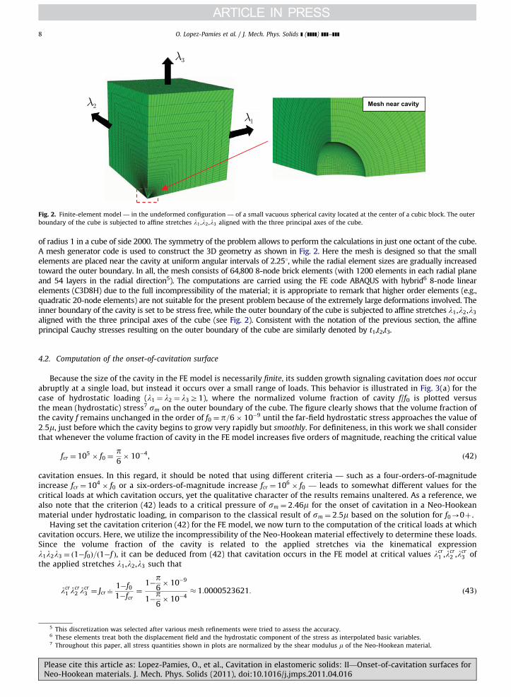
Fig. 2. Finite-element model — in the undeformed configuration — of a small vacuous spherical cavity located at the center of a cubic block. The outer

boundary of the cube is subjected to affine stretches l1 ,l2 ,l3 aligned with the three principal axes of the cube.


of radius 1 in a cube of side 2000. The symmetry of the problem allows to perform the calculations in just one octant of the cube.A mesh generator code is used to construct the 3D geometry as shown in Fig. 2. Here the mesh is designed so that the smallelements are placed near the cavity at uniform angular intervals of 2.251, while the radial element sizes are gradually increasedtoward the outer boundary. In all, the mesh consists of 64,800 8-node brick elements (with 1200 elements in each radial planeand 54 layers in the radial direction5). The computations are carried using the FE code ABAQUS with hybrid6 8-node linearelements (C3D8H) due to the full incompressibility of the material; it is appropriate to remark that higher order elements (e.g.,quadratic 20-node elements) are not suitable for the present problem because of the extremely large deformations involved. Theinner boundary of the cavity is set to be stress free, while the outer boundary of the cube is subjected to affine stretches l1,l2,l3

aligned with the three principal axes of the cube (see Fig. 2). Consistent with the notation of the previous section, the affineprincipal Cauchy stresses resulting on the outer boundary of the cube are similarly denoted by t1,t2,t3.

4.2. Computation of the onset-of-cavitation surface

Because the size of the cavity in the FE model is necessarily finite, its sudden growth signaling cavitation does not occurabruptly at a single load, but instead it occurs over a small range of loads. This behavior is illustrated in Fig. 3(a) for thecase of hydrostatic loading (l1 ¼ l2 ¼ l3Z1), where the normalized volume fraction of cavity f/f0 is plotted versusthe mean (hydrostatic) stress7 sm on the outer boundary of the cube. The figure clearly shows that the volume fraction ofthe cavity f remains unchanged in the order of f0 ¼ p=6� 10�9 until the far-field hydrostatic stress approaches the value of2:5m, just before which the cavity begins to grow very rapidly but smoothly. For definiteness, in this work we shall considerthat whenever the volume fraction of cavity in the FE model increases five orders of magnitude, reaching the critical value

fcr ¼ 105� f0 ¼

p6� 10�4, ð42Þ

cavitation ensues. In this regard, it should be noted that using different criteria — such as a four-orders-of-magnitudeincrease fcr ¼ 104

� f0 or a six-orders-of-magnitude increase fcr ¼ 106� f0 — leads to somewhat different values for the

critical loads at which cavitation occurs, yet the qualitative character of the results remains unaltered. As a reference, wealso note that the criterion (42) leads to a critical pressure of sm ¼ 2:46m for the onset of cavitation in a Neo-Hookeanmaterial under hydrostatic loading, in comparison to the classical result of sm ¼ 2:5m based on the solution for f0-0þ .

Having set the cavitation criterion (42) for the FE model, we now turn to the computation of the critical loads at whichcavitation occurs. Here, we utilize the incompressibility of the Neo-Hookean material effectively to determine these loads.Since the volume fraction of the cavity is related to the applied stretches via the kinematical expressionl1l2l3 ¼ ð1�f0Þ=ð1�f Þ, it can be deduced from (42) that cavitation occurs in the FE model at critical values lcr

1 ,lcr2 ,lcr

3 ofthe applied stretches l1,l2,l3 such that

lcr1 l

cr2 l

cr3 ¼ Jcr6

1�f0

1�fcr¼

1�p6� 10�9

1�p6� 10�4

� 1:0000523621: ð43Þ

5 This discretization was selected after various mesh refinements were tried to assess the accuracy.6 These elements treat both the displacement field and the hydrostatic component of the stress as interpolated basic variables.7 Throughout this paper, all stress quantities shown in plots are normalized by the shear modulus m of the Neo-Hookean material.


dx.doi.org/10.1016/j.jmps.2011.04.016

1

5x10

1x10

0 0.5 1 1.5 2 2.5 3

Fig. 3. (a) Increase in the volume fraction f of cavity in the FE model, as a function of the far-field mean (hydrostatic) stress sm , for the case of hydrostatic

loading with l1 ¼ l2 ¼ l3 Z1. (b) FE solutions for the hydrostatic stress sm versus the shear stresses t1 and t2 that result on the outer boundary of the

cube by marching along the two-step loading process (44)–(45) for three values of the parameter m. The stresses associated with Step II correspond to

the critical stresses at which cavitation ensues.


The critical values tcr1 , tcr

2 , tcr3 of the corresponding principal Cauchy stresses t1, t2, t3 on the outer boundary of the cube can

then be found by marching along (starting at l1 ¼ l2 ¼ l3 ¼ 1) volume-increasing loading paths in (l1,l2,l3)-space untilthe product l1l2l3 reaches the value (43). An alternative, more efficient strategy is to first subject the cube to hydrostaticloading until condition (43) is reached, and then vary the ratios of the stretches l1=l2 and l2=l3 while keeping theirproduct fixed at the cavitated state l1l2l3 ¼ Jcr in such a way that the critical stresses tcr

1 , tcr2 , tcr

3 are computed continuouslyalong the loading path. A convenient parameterization of this two-step loading process is as follows:

Step I : l1 ¼ l2 ¼ l3 ¼ l for 1rlr J1=3cr ð44Þ

and

Step II : l1 ¼ l, l2 ¼ lm, l3 ¼ Jcrl�ð1þmÞ for l4 J1=3

cr , ð45Þ

where l is a monotonically increasing load parameter that takes the value of 1 in the undeformed configuration and m 2 R,but because of symmetry it actually suffices to restrict attention to m 2 ½�0:5,1�. Fig. 3(b) shows FE solutions for theprincipal Cauchy stresses t1, t2, t3 on the outer boundary of the cube that result by marching along the above two-steploading process for the cases of m¼�0.5,0, and 1; for each m in Step II, the computation is restarted from the hydrostaticloading results of Step I. For consistency with the next section, the results are plotted in terms of the hydrostatic stresssm ¼ 1=3ðt1þt2þt3Þ as a function of the shear stresses t1 ¼ t2�t1 and t2 ¼ t3�t1. Note that the stresses associated withStep II of the loading process correspond precisely to the critical stresses at which cavitation ensues. The entire onset-of-cavitation surface can then be constructed by simply carrying out more calculations for various values of m 2 ½�0:5,1�.

5. Onset-of-cavitation surfaces and discussion

We present here results of the onset-of-cavitation surfaces worked out in Sections 3 and 4, as well as of some earlierresults available in the literature. In the first set of plots, we focus on the case of axisymmetric loading conditions. As it willbecome apparent below, this special case serves to illustrate in a ‘‘two-dimensional’’ setting all the main effects that loadtriaxiality — namely, the departure from pure hydrostatic loading — has on the onset of cavitation in Neo-Hookeanmaterials. The second set of plots pertains to the entire onset-of-cavitation surfaces for general loading conditions.

5.1. Axisymmetric loading

Fig. 4 shows plots for the hydrostatic stress sm and shear stress t1 at which cavitation ensues in Neo-Hookean materialsunder axisymmetric loading conditions with t2 ¼ t1 (recall the definition (38)). The solid line corresponds to thetheoretical result (40) derived in Section 3, while the solid circles denote the FE results generated in Section 4. The figurealso includes the variational approximation (dashed line) of Hou and Abeyaratne (1992) and the earlier numerical results(triangles) of Chang et al. (1993) based on an allegedly equivalent8 2D axisymmetric FE model.

A key observation from Fig. 4 is that cavitation occurs only at states of axisymmetric stress for which the hydrostaticpart sm is tensile, in accordance with experiments. For all four results, the critical value of sm is lowest for purelyhydrostatic loading when t1 ¼ 0, and increases significantly and monotonically as the shear stress t1 deviates from

8 Chang et al. (1993) examined the problem of a pressurized cavity in a cylindrical block under uniaxial tension and considered it as equivalent to the

problem of a vacuous cavity in a cylindrical block under multi-axial tension.


dx.doi.org/10.1016/j.jmps.2011.04.016

0

2

4

6

8

10

-12 -8 -4 0 4 8 12

Fig. 4. Onset-of-cavitation curves for Neo-Hookean materials under axisymmetric loading with t2 ¼ t1 in the space of (sm ,t1)-stress. The solid line

corresponds to the theoretical result (40), the solid circles correspond to the FE results generated in Section 4, the dashed line indicates the variational

approximation of Hou and Abeyaratne (1992), and the triangles denote the earlier FE results of Chang et al. (1993).


zero—that is, as the load triaxiality decreases. Note in particular that the critical sm increases faster for loadings witht140, which correspond to the case when the two principal Cauchy stresses that are equal (t2 and t3 in this case) aregreater than the other principal Cauchy stress (t1 in this case).

Another key observation from Fig. 4 is that the FE cavitation results generated in Section 4 are in fairly good agreementwith the theoretical onset-of-cavitation curve (40). This is a remarkable connection given that the FE results are based onthe growth of a single spherical cavity, while the theoretical result (40) is based on the growth of an isotropic distribution of

cavities. This agreement thus suggests that the interaction among cavities may not play an important role in the onset ofcavitation in elastomeric solids. Further evidence supporting this possibility has been provided by the recent work of Xuand Henao (in press), who have shown — in the context of a class of 2D compressible isotropic elastic solids — that thecritical load at which cavitation ensues based on the growth of an isolated defect is essentially the same as that based onthe growth of two neighboring defects. This issue is worth of further study in more general material systems.

Finally, we remark from Fig. 4 that the variational approximation of Hou and Abeyaratne (1992) has the samequalitative behavior as the theoretical result (40). Quantitatively, it agrees with (40) for purely hydrostatic loading (t1 ¼ 0),but predicts much larger critical stresses for the onset of cavitation as the shear stress t1 deviates from 0. This behavior isconsistent with the fact that their approximation was constructed by making use of a kinematically admissible trial field incertain energy minimization problem, thus leading to overpredictions for the actual critical stresses at cavitation.9 We alsoremark that the FE results of Chang et al. (1993) are in agreement with our FE results — and therefore with the theoreticalresult (40) — except for loadings with large positive shear stress t1. It should be noted, however, that the equivalencybetween the two FE approaches remains to be verified.

5.2. General loading

Fig. 5(a) displays the onset-of-cavitation surface (39) for Neo-Hookean materials under 3D loading conditions witharbitrary triaxiality. The surface is plotted in terms of the hydrostatic stress sm as a function of the shear stresses t1 and t2

at which cavitation ensues. The overall features of the surface are seen to be identical to those of the onset-of-cavitationcurve shown in Fig. 4 for the case of axisymmetric loading. Namely, cavitation occurs only at states of stress for which thehydrostatic part sm is tensile. Moreover, the critical value of sm is lowest for purely hydrostatic loading when t1 ¼ t2 ¼ 0,and increases significantly and monotonically as the shear stresses t1 and t2 deviate from zero in any radial path—that is,as the load triaxiality decreases. Making use of an approximate linear-comparison technique in the correspondingtwo-dimensional problem, Lopez-Pamies (2009) found this same trend of increasing sm with decreasing load triaxiality forcompressible Neo-Hookean materials. However, he also found that other classes of compressible materials exhibit the exactopposite trend (see Section 5.2, Lopez-Pamies, 2009). The question arises then as to whether the ‘‘exact’’ theory proposedin Part I confirms such trends. This issue, which can have strong practical implications, will be investigated in future work.

Fig. 5(b) compares the theoretical surface (39) with the onset-of-cavitation surface generated from the FE results ofSection 4; for clarity of presentation, only results in the quadrant of negative shear stresses t1 and t2 are included in the

9 Specifically, their result constitutes a rigorous upper bound for the critical far-field stresses at which a single vacuous spherical cavity embedded in

an infinite Neo-Hookean medium suddenly grows unbounded.


dx.doi.org/10.1016/j.jmps.2011.04.016

50

55

05

0

5

10

Fig. 5. (a) 3D plot of the theoretical onset-of-cavitation surface (39) for Neo-Hookean materials in the space of (sm ,t1 ,t2)-stress. (b) Comparison of (39)

with the onset-of-cavitation surface generated from the FE results of Section 4.


figure. The FE surface is seen to be identical in form to the theoretical surface. The quantitative agreement is alsoremarkably good—in spite of the fact, again, that the FE results are based on the growth of a single spherical cavity, whilethe theoretical result (40) is based on the growth of an isotropic distribution of cavities. Much like in the case ofaxisymmetric loading shown in Fig. 4 (which corresponds to the line t2 ¼ t1 in this plot) the FE results are seen to predictsimilar, but progressively higher hydrostatic stresses as the load triaxiality decreases (i.e., as t1 and t2 deviate from zero),for the onset of cavitation in Neo-Hookean materials.

In summary, the above results indicate that Neo-Hookean solids significantly improve their stability — in the sense thatcavitation takes place at larger mean (hydrostatic) stresses — with decreasing load triaxiality. This has strong practicalimplications. For instance, in the contexts of filled elastomers (Gent and Park, 1984; Cho et al., 1987; Moraleda et al., 2009;Michel et al., 2010) and structures bonded by soft adhesives (Creton and Hooker, 2001), the regions surrounding theinherent soft/stiff interfaces are known to develop high stress triaxialities and therefore are prone to cavitation. Yet thestress states in these regions are not purely hydrostatic but do involve sizable shear stresses. Predictions based uponradially symmetric cavitation ignoring the effect of shear stresses in these material systems may then result in substantialerrors, and may even lead to incorrect conclusions. In the context of rubber-toughened polymers (Cheng et al., 1995;Steenbrink and Van der Giessen, 1999), the underlying rubber particles also develop states of high — but not purely —

hydrostatic stress. Ignoring the effect of shear stresses on the onset of cavitation in this case may also lead to incorrectconclusions.

6. An approximate closed-form cavitation criterion for Neo-Hookean materials

The cavitation criterion (31) requires knowledge of the function C defined by (32), which ultimately amounts to solvingnumerically the pde (75) subject to the initial condition (76). In this section, we propose an approximate criterion which isclosed form and very close to the exact criterion (31).

The approximation is based on the observation that the function C takes the value 1 for purely hydrostatic loading anddecays slowly to zero with decreasing load triaxiality, as described by the properties (35)–(37) and illustrated graphicallyin Fig. 1(b). Thus, we can generate an approximate criterion that agrees exactly with the exact criterion (31) at thehydrostatic point by simply taking the function C equal to 1 in (31). The result is given by

SBðt1,t2,t3Þ ¼ 8t1t2t3�12mðt1t2þt1t3þt2t3Þþ18m2ðt1þt2þt3Þ�35m3 ¼ 0, ð46Þ

where only the root with ti40 (i¼1,2,3) ought to be selected. In the space of stress measures (38), this approximatecriterion takes the form

SBðsm,t1,t2Þ ¼ 8ð3sm�t1�t2Þð3smþ2t1�t2Þð3smþ2t2�t1Þ�108mð9s2m�t

21�t

22þt1t2Þþ1458m2sm�945m3 ¼ 0,

ð47Þ

where only the root with sm43m=2þ1=3ðt1þt2Þ, sm43m=2þ1=3ðt1�2t2Þ, and sm43m=2þ1=3ðt2�2t1Þ ought to beselected. It is easy to verify that these surfaces contain the hydrostatic point (41).

Fig. 6 provides comparisons between the exact surface (39) — shown in solid lines — and its closed-formapproximation (47) — shown in dotted lines — in the space of (sm,t1,t2)-stress. Part (a) shows plots for axisymmetricloading with t2 ¼ t1, in which case the approximate surface (47) reduces to the curve

SBðsm,t1,t1Þ ¼ sm�3m2�

24=3t21þ 4t3

1þ54m3þ6ffiffiffiffiffiffiffiffiffiffiffiffiffiffiffiffiffiffiffiffiffiffiffiffiffiffiffiffiffiffiffiffi81m6þ12m3t3

1

q� �2=3

6 2t31þ27m3þ3

ffiffiffiffiffiffiffiffiffiffiffiffiffiffiffiffiffiffiffiffiffiffiffiffiffiffiffiffiffiffiffiffi81m6þ12m3t3

1

q� �1=3¼ 0: ð48Þ


dx.doi.org/10.1016/j.jmps.2011.04.016

0

2

4

6

8

10

-12 -8 -4 0 4 8 12

Fig. 6. Comparisons between the exact onset-of-cavitation surface (39) and its closed-form approximation (47). Part (a) shows results for the

hydrostatic stress sm as a function of the shear stress t1 for the special case of axisymmetric loading with t2 ¼ t1, while part (b) shows contour lines of

sm as a function of t1 and t2 for general loading conditions. In both parts, the solid lines correspond to the exact surface (39) and the dashed lines to its

closed-form approximation (47).


The comparisons show that, indeed, the approximate curve agrees exactly with the exact curve at the hydrostatic point(t1 ¼ 0) and remains remarkably close to the exact curve over a large range of shear stresses t1. Comparisons for generalloading conditions are provided in part (b). This figure shows contour lines of hydrostatic stress sm in the space of shearstresses (t1,t2). Once again, the approximate surface is seen to reproduce remarkably accurately the exact surface for theentire large range of shear stresses t1 and t2 considered.

Fig. 6 also shows that the approximate surface always lies ‘‘outside’’ the exact surface (relative to the origin). In fact, theapproximate surfaces (46) and (47) can be shown to be rigorous outer bounds for the corresponding exact surfaces (31)and (39). To see this, note that in view of the relations (29), (30), and (38) any stress state lying on the exact surface (39)can be written parametrically as

t1 ¼ mðl22�l

21Þ, t2 ¼ m

1

l21l

22

�l21

!, sm ¼ m l2

1þl22þ

1

l21l

22

!þ

9

2mF l1

l2,l1l

22

� �, ð49Þ

where the parameters l1 2 ð0,þ1Þ and l2 2 ð0,þ1Þ. By the same token, any stress state lying on the approximate surfaceSB can be written in similar form but with F¼C¼ 1, namely,

tB1 ¼ mðl

22�l

21Þ, tB

2 ¼ m1

l21l

22

�l21

!, sB

m ¼ m l21þl

22þ

1

l21l

22

!þ

9

2m, ð50Þ

where we have utilized the superscript ‘‘B’’ to avoid notational confusion. Given that the maximum value of F is 1 (seeEq. (25)), for any pair of parameters l1 and l2 we have that t1 ¼ tB

1, t2 ¼ tB2 and smrsB

m, and therefore that theapproximate surface SB bounds from outside the exact surface S. From the definition of the stress measures (38), it thenfollows that the approximate surface SB also bounds from outside the exact surface S in the space of (t1, t2, t3)-stress.

The approximate condition (46) provides then an accurate and mathematically simple cavitation criterion — which canbe utilized in lieu of (31) for practical purposes — for Neo-Hookean solids under general loading conditions.

Acknowledgments

Support for this work by the National Science Foundation (USA) through Grant DMS-1009503 is gratefully acknowl-edged. M.I.I. would also like to acknowledge support from CONICET (Argentina) under Grant PIP 00394/10.

Appendix A. Derivation of the initial-value problem (20)–(21) for E

This appendix provides the main steps in the derivation of Eqs. (20) and (21), which correspond to the specialization ofthe initial-value problem (15) to the case of Neo-Hookean materials with stored-energy function (18). We begin bycomputing the inversion of relations (19)

l1 ¼L2=31 L1=3

2 J1=3, l2 ¼L1=3

2 J1=3

L1=31

, l3 ¼J1=3

L1=31 L2=3

2

, ð51Þ


dx.doi.org/10.1016/j.jmps.2011.04.016


and recognize, by using the definition EðL1,L2,J,f0Þ6Eðl1,l2,l3,f0Þ and the chain rule, that

@E

@l1¼

L1=31

L1=32 J1=3

@E

@L1þ

J2=3

L2=31 L1=3

2

@E

@J,

@E

@l2¼�

L4=31

L1=32 J1=3

@E

@L1þL1=3

1 L2=32

J1=3

@E

@L2þL1=3

1 J2=3

L1=32

@E

@J,

@E

@l3¼�

L1=31 L5=3

2

J1=3

@E

@L2þL1=3

1 L2=32 J2=3 @E

@J: ð52Þ

With the help of expressions (51) and (52), and in view of the linearity of (18) in the sum of the squares of the principalstretches l2

1þl22þl

23, it is then straightforward to compute the corresponding maximizing vector x in (15). The solution

reads (in component form) as

o1 ¼�L2=3

1 L1=32 x1½JðL

21ðL

22x

23þx

22Þþx

21Þ�1�

J2=3½L21ðL

22x

23þx

22Þþx

21�

þL7=3

1 x1ðL22x

23þ2x2

2Þ

L1=32 J1=3m½L2

1ðL22x

23þx

22Þþx

21�

@E

@L1þ

L4=31 L2=3

2 x1ðL22x

23�x

22Þ

J1=3m½L21ðL

22x

23þx

22Þþx

21�

@E

@L2,

o2 ¼�L1=3

2 x2½L21ðJðL

22x

23þx

22Þ�1Þþ Jx2

1�

L1=31 J2=3½L2

1ðL22x

23þx

22Þþx

21��

L4=31 x2ðL

21L

22x

23þ2x2

1Þ

L1=32 J1=3m½L2

1ðL22x

23þx

22Þþx

21�

@E

@L1þL1=3

1 L2=32 x2½2L

21L

22x

23þx

21�

J1=3m½L21ðL

22x

23þx

22Þþx

21�

@E

@L2,

o3 ¼1�J

L1=31 L2=3

2 J2=3x3

�x1o1

L1L2x3�x2o2

L2x3: ð53Þ

By making direct use of the explicit expressions (53), it is possible to carry out analytically the resulting integrals in (15). Inturn, after some algebraic manipulations, the initial-value problem (15) can be finally rewritten as Eqs. (20) and (21) in themain body of the text, where

G0ðL1,L2,JÞ ¼�3

2þ

J2=3½ðL21þ1ÞL2

2þ1�

3L2=31 L4=3

2

þL1=3

1 L2=32

2J4=3GF ,

G1ðL1,L2Þ ¼L3

1þL1

L21�1

�L2

1½ðL21þ1ÞL2

2�2�

ðL21�1ÞðL2

1L22�1Þ

GEþL2

1L22

1�L21L

22

GF ,

G2ðL1,L2Þ ¼�L2

1L2

L21�1þL1L2½ð2L2

1�1ÞL22�1�

ðL21�1ÞðL2

1L22�1Þ

GEþL1L3

2

1�L21L

22

GF ,

G3ðL1,L2Þ ¼L5=3

1 L1=32 ½�ð5L

21þ3ÞL2

2þ2ðL21þ1Þþð�2L6

1þ4L41þL

21þ1ÞL4

2�

3ðL21�1Þ2ðL2

2�1ÞðL21L

22�1Þ

�L8=3

1 L1=32 ½ðL

21�2ÞL2

2þ1�½L22ð4L

41L

22�L

21ðL

22þ7ÞþL2

2�1Þþ4�

3ðL21�1Þ2ð1�L2

2ÞðL21L

22�1Þ2

GE

þ2L8=3

1 L7=32 ½�ðL

21þ1ÞL2

2þðL41�L

21þ1ÞL4

2þ1�

3ðL21�1Þð1�L2

2ÞðL21L

22�1Þ2

GF ,

G4ðL1,L2Þ ¼L8=3

1 ½ðL21þ3Þð3L2

1þ1ÞL22�4ðL2

1þ1ÞþðL61�5L4

1�5L21þ1ÞL4

2�

6ðL21�1Þ2L2=3

2 ðL22�1ÞðL2

1L22�1Þ

þL11=3

1 ½12L21L

42�6ðL2

1þ1ÞL22þðL

21þ1ÞðL4

1�4L21þ1ÞL6

2þ4�

3ðL21�1Þ2L2=3

2 ð1�L22ÞðL

21L

22�1Þ2

GE

�L11=3

1 L4=32 ½�ð7L

21þ1ÞL2

2þðL41þ5L2

1�2ÞL42þ4�

6ðL21�1Þð1�L2

2ÞðL21L

22�1Þ2

GF ,

G5ðL1,L2Þ ¼L2=3

1 L4=32 ðL

21ð7�3L2

1ÞL22�L

21þð4L

61�5L4

1�2L21þ1ÞL4

2�1Þ

6ðL21�1Þ2ðL2

2�1ÞðL21L

22�1Þ

þL5=3

1 L4=32 ðð4L

61�6L4

1þ1ÞL62�3ð2L4

1�4L21þ1ÞL4

2�3L22þ1Þ

3ðL21�1Þ2ð1�L2

2ÞðL21L

22�1Þ2

GE

�L5=3

1 L10=32 ðð5�7L2

1ÞL22þð4L

41�L

21�2ÞL4

2þ1Þ

6ðL21�1Þð1�L2

2ÞðL21L

22�1Þ2

GF : ð54Þ


dx.doi.org/10.1016/j.jmps.2011.04.016


In the above coefficients,

GF ¼1ffiffiffiffiffiffiffiffiffiffiffiffiffi

1�L22

q EF

ffiffiffiffiffiffiffiffiffiffiffiffiffi1�L2

2

q2

ffiffiffiffiffiffiffiffiffiffiffiffiffiL2

2�1q ln½2L2ðL2þ


2�1q

Þ�1�;L2

1L22�1

L22�1

264

375,

GE ¼1ffiffiffiffiffiffiffiffiffiffiffiffiffi

1�L22

q EE


2

q2




2�1q

Þ�1�;L2

1L22�1

L22�1

264

375, ð55Þ

where the functions EF and EE stand for, respectively, the elliptic integrals of first and second kind, as defined by

EF ½j; k� ¼Z j

0½1�k sin2 y��1=2 dy and EE ½j; k� ¼

Z j

0½1�k sin2 y�1=2 dy: ð56Þ

Appendix B. Asymptotic solution to (20)–(21) in the limit as f0-0þ

In order to solve asymptotically the initial-value problem (20)–(21) for vanishingly small values of f0, first it isimportant to recognize that the initial condition (21) is given at f0¼1, which corresponds to the opposite end to theneighborhood around f0¼0 in the range of physical volume fraction of cavities f0 2 ½0,1�. Thus, assuming a certain ansatzfor E near f0¼0 and then expanding the nonlinear pde (20) near f0¼0 — as usually done to solve asymptotic problems — isexpected to generate a nested10 system of equations for the coefficients introduced in the ansatz. Indeed, this structure isexpected to occur because the solution to the initial-value problem (20)–(21) near f0¼0 depends, of course, on the initialcondition (21) which is given at f0¼1, far away from the neighborhood around f0¼0. In practice, this means that thecomputation of the asymptotic solution to (20)–(21) near f0¼0 may require, in general, the computation of the fullsolution to (20)–(21) for all f0 2 ½0,1�. Because of the isotropy of the total elastic energy E at hand, however, it is possible toconstruct an asymptotic solution to (20)–(21) near f0¼0 without having to compute the entire solution for all f0, which isobviously a much more involved task. As elaborated in this appendix, the idea is to consider successively the cases ofhydrostatic (L1 ¼L2 ¼ 1), axisymmetric (L2 ¼ 1), and general loading conditions, in such a manner that the appropriateinitial conditions for the resulting pdes can be written in terms of the deformation variables (L1 and L2) instead of interms of the initial volume fraction of cavities (f0).

(I) Hydrostatic loading conditions: Thus, we begin by analyzing the special case of hydrostatic loading conditions when

L1 ¼L2 ¼ 1: ð57Þ

For this type of loading, we note that isotropy dictates that

@E

@L1ð1,1,J,f0Þ ¼

@E

@L2ð1,1,J,f0Þ ¼ 0, ð58Þ

which, after defining EHðJ,f0Þ6Eð1,1,J,f0Þ, allows to simplify the problem (20)–(21) to the form

f0@E

H

@f0�EþðJ�1Þ

@EH

@Jþm2

2J2=3þ1

J4=3�3

� �¼ 0, E

HðJ,1Þ ¼ 0: ð59Þ

The initial-value problem (59) admits the following closed-form solution:

EHðJ,f0Þ ¼

3m2

2J�1

J1=3�

2Jþ f0�2

ðJþ f0�1Þ1=3f 1=30 �ð1�f0Þ

" #: ð60Þ

Note that this solution is valid for any f0 2 ½0,1�. When f0-0þ , (60) reduces asymptotically to

EHðJ,f0Þ ¼

3m2

2J�1

J1=3�1

� ��3mðJ�1Þ2=3f 1=3

0 þOðf0Þ: ð61Þ

(II) Axisymmetric loading conditions: Next, we consider the case of axisymmetric loading conditions with

L2 ¼ 1: ð62Þ

Again, by exploiting isotropy we have the connection

@E

@L2ðL1,1,J,f0Þ ¼

L1

2

@E

@L1ðL1,1,J,f0Þ, ð63Þ

10 That is, the solution for the coefficient of first order depends on the solution for the coefficient of second order, which in turn depends on the

solution for the coefficient of third order, and so on so forth.


dx.doi.org/10.1016/j.jmps.2011.04.016


which, after defining EAðL1,J,f0Þ6EðL1,1,J,f0Þ, allows to reduce (20)–(21) to the simpler initial-value problem

f0@E

A

@f0�E

A�

3m2þð2þL2

1Þð1þ2J2Þm6L2=3

1 J4=3�

3L8=31 ð2ðL

21þ2Þ


1�1q

�3L1ln½2L21þL1


1�1q

�1�Þ

16mðL21�1Þ5=2J2=3

�2mðL2

1�1Þ

3L5=31 J1=3

�@E

A

@L1

!2

þðJ�1Þ@E

A

@J¼ 0, E

AðL1,J,1Þ ¼ 0: ð64Þ

As opposed to the problem of hydrostatic loading (59), the problem of axisymmetric loading (64) does not seem to admit aclosed-form solution for all f0 2 ½0,1�. However, a numerical solution can be readily computed. Then, utilizing the fullnumerical solution as a guide, the behavior of E

AðL1,J,f0Þ in the limit as f0-0þ can be assumed to be of the asymptotic

form

EAðL1,J,f0Þ ¼ E

A

0ðL1,JÞþ EA

1ðL1,JÞf 1=30 þOðf 2=3

0 Þ: ð65Þ

Substituting this ansatz in the pde (64)1 and expanding around f0¼0 leads to a hierarchical system of pdes for EA

0, EA

1, andhigher-order coefficients. The first equation of this system, of order O(1), reads as

�EA

0�3m2þð2þL2

1Þð1þ2J2Þm6L2=3

1 J4=3�

3L8=31 ð2ðL

21þ2Þ


1�1q

�3L1ln½2L21þL1


1�1q

�1�Þ

16mðL21�1Þ5=2J2=3

�2mðL2

1�1Þ

3L5=31 J1=3

�@E

A

0

@L1

!2

þðJ�1Þ@E

A

0

@J¼ 0: ð66Þ

Now, by recognizing that EAð1,J,f0Þ ¼ E

HðJ,f0Þ, we conclude from (61) that

EA

0ð1,JÞ ¼3m2

2J�1

J1=3�1

� �, ð67Þ

which can be viewed as the initial condition for the pde (66). The solution to the initial-value problem (66)–(67) can thenbe computed to lead to

EA

0ðL1,JÞ ¼m2

J2=3 ð2þL21Þ

L2=31

�3

" #þ

3m2

ðJ�1Þ

J1=3FAðL1Þ, ð68Þ

where the function FA is a solution to the ode

FA�L2

1þ2

2L2=31

þ27L8=3

1

32ðL21�1Þ5=2

½2ðL21þ2Þ


1�1q

�3L1ln½2L21þ2L1


1�1q

�1��4ðL2

1�1Þ

9L5=31

þdFA

dL1

!2

¼ 0, ð69Þ


FAð1Þ ¼ 1: ð70Þ

Having solved for EA

0, the coefficient EA

1 can then be determined from the second equation of the hierarchical system, oforder O(f0

1/3), subject to the initial condition E

A

1ð1,JÞ ¼�mðJ�1Þ2=3, as dictated by (61). Given that EA

1, and the remaininghigher-order coefficients in the ansatz (65), are not needed for our purposes, its computation is omitted here.

(III) General loading conditions: Finally, we consider the case of general loading conditions. In the limit as f0-0þ , weassume the total elastic energy to be of the asymptotic form

EðL1,L2,J,f0Þ ¼ E0ðL1,L2,JÞþ E1ðL1,L2,JÞf 1=30 þOðf 2=3

0 Þ: ð71Þ

Substituting this ansatz in the pde (20) and expanding around f0¼0 leads to a hierarchical system of pdes for E0, E1 andhigher-order coefficients. The leading order term of these equations, of order O(1), reads as

�E0þðJ�1Þ@E0

@JþG0ðL1,L2,JÞþ

1

JG1ðL1,L2Þ

@E0

@L1þ

1

JG2ðL1,L2Þ

@E0

@L2

þ1

J2=3G3ðL1,L2Þ

@E0

@L1

@E0

@L2þ

1

J2=3G4ðL1,L2Þ

@E0

@L1

!2

þ1

J2=3G5ðL1,L2Þ

@E0

@L2

!2

¼ 0, ð72Þ

where it is recalled that the coefficients G0, G1, G2, G3, G4, G5 are given explicitly by (54). At this stage, we recognize thatEðL1,1,J,f0Þ ¼ E

AðL1,J,f0Þ, and hence that

E0ðL1,1,JÞ ¼ EA

0ðL1,JÞ, ð73Þ

with EA

0 denoting the leading order term (68) of the asymptotic axisymmetric solution (65) worked out above. Expression(73) can be considered as the initial condition for the pde (72). The solution to the initial-value problem (72)–(73) can be


dx.doi.org/10.1016/j.jmps.2011.04.016


worked out analytically to render

E0 ¼m2

J2=3 ðL21þ1ÞL2

2þ1

L2=31 L4=3

2

�3

" #þ

3m2

ðJ�1Þ

J1=3FðL1,L2Þ, ð74Þ

where F is the solution to the following first-order nonlinear pde:

F ðL1,L2ÞFþF 0ðL1,L2ÞþF1ðL1,L2Þ@F@L1þF2ðL1,L2Þ

@F@L2þF3ðL1,L2Þ

@F@L1

@F@L2

þF 4ðL1,L2Þ@F@L1

� �2

þF5ðL1,L2Þ@F@L2

� �2

¼ 0 ð75Þ


FðL1,1Þ ¼FAðL1Þ: ð76Þ

In the above expressions, the coefficients are given by

F ðL1,L2Þ ¼ �4ðL21�1Þ2L2=3

2 ðL22�1ÞðL2

1L22�1Þ2,

F 0ðL1,L2Þ ¼ 4L1=31 ðL

21�1Þ2L4=3

2 ðL22�1ÞðL2

1L22�1Þ2GF ,

F 1ðL1,L2Þ ¼ 12L1ðL21�1ÞL2=3

2 ðL22�1ÞðL2

1L22�1Þ ½�L1L2

2ð�L21ðGEþGF Þ�GEþGFþL3

1þL1Þ�2GEL1þL21þ1�,

F 2ðL1,L2Þ ¼ 12L1ðL21�1ÞL5=3

2 ðL22�1ÞðL2

1L22�1Þ ½L2

2ð�2GEL21þGEþGF ðL2

1�1ÞþL31ÞþGE�L1�,

F 3ðL1,L2Þ ¼ 6L5=31 L2½GEL1ððL2

1�2ÞL22þ1ÞðL2

2ð4L41L

22�L

21ðL

22þ7ÞþL2

2�1Þþ4Þ

þL22ðL1ð2ð�GFL2

1þGFþL31Þþ7L1Þþ3ÞþL4

2ð2GF ðL41�1ÞL1þ2L6

1�9L41�1�4L2

1Þ

þL1L62ð�2GF ðL6

1�2L41þ2L2

1�1Þ�2L71þ4L5

1þL31þL1Þ�2ðL2

1þ1Þ�,

F 4ðL1,L2Þ ¼ 3L8=31 ½L

22ð12GEðL3

1þL1Þþ4GF ðL21�1ÞL1�7ðL2

1þ2ÞL21�3ÞþL4

2

�ðL1ð6L21ðGF�4GEÞ�7GFL4

1þGFþ2L51þ15L3

1þ8L1Þ�1ÞþL1L62ð�2GE

�ðL21þ1ÞðL4

1�4L21þ1ÞþGF ðL6

1þ4L41�7L2

1þ2ÞþL71�5L5

1�5L31þL1Þþ4L1ðL1�2GEÞþ4�,

F 5ðL1,L2Þ ¼ 3L2=31 L2

2½L1L22ð6GEþGF ðL2

1�1Þþ2L1ðL21�4ÞÞþL4

2

�ðL1ð6GEð2L41�4L2

1þ1Þþð7L21�12ÞL2

1ð�ðGFþL1ÞÞ�5GFþ2L1Þ�1Þ

þL1L62ð�2GEð4L6

1�6L41þ1Þ�GF ðL2

1�2Þþð4L21�5ÞL4

1ðGFþL1Þ�2L31þL1Þ�2GEL1þL

21þ1�, ð77Þ

and it is recalled that the function FA is defined by the initial-value problem (69)–(70), and that GF and GE are defined byexpressions (55).

While the function F, as defined by the initial-value problem (75)–(76), cannot be written in the closed form, it isrelatively simple to compute it numerically. In Appendix C below, we spell out the key steps in the numerical computationof F and discuss its properties.

Appendix C. The function UðL1L2Þ

In this appendix, we discuss the numerical computation of the function F defined by the initial-value problem(75)–(76), as well as establish its growth conditions and upper and lower bounds.

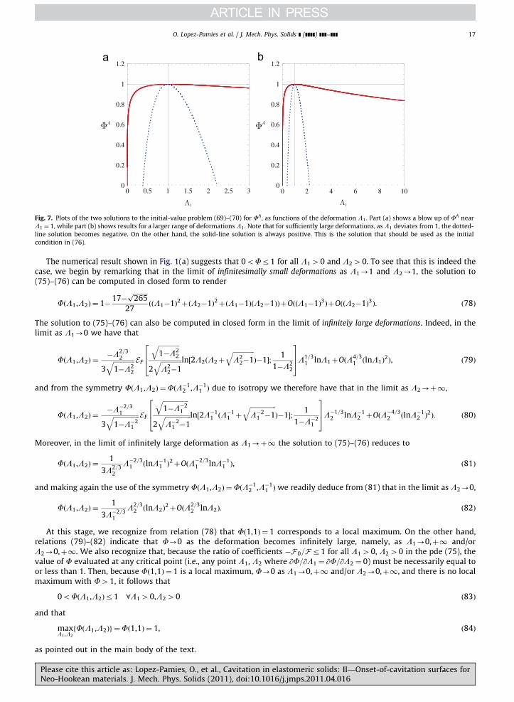
The numerical computation of F requires solving the first-order nonlinear pde (75) subject to the initial condition (76).In this regard, we note that the initial condition (76) itself requires solving numerically the nonlinear ode (69) subject tothe initial condition (70). Now, because of its quadratic nonlinearity, it is important to realize that Eq. (76) has twosolutions. One of the solutions is always positive, whereas the other solution is unbounded from below and can thereforebe negative, as illustrated by Fig. 7. Given that the total energy (74) of the material must be nonnegative, we discard theunbounded solution (i.e., the dotted-line curve in Fig. 7) as non-physical, and utilize the positive solution (i.e., the solid-line curve in Fig. 7) as the initial condition in (76). In a parallel note, we remark that similar care should be exercised inselecting the appropriate solution when dealing with materials other than Neo-Hookean.

Having identified which is the function FA that must be utilized in (76), we are now in a position to computenumerically the solution for F. As a result of our choice of FA, in spite of its quadratic nonlinearity, the pde (75) subject to(76) has only one solution for F. Fig. 1(a) shows a plot for that solution in a large range of deformations L1 and L2.An important observation from this plot is that in the undeformed configuration (i.e., when L1 ¼L2 ¼ 1) F¼ 1,and that beyond the undeformed configuration (i.e., as L1 and L2 deviate from 1), F decreases monotonically alongany radial path.


dx.doi.org/10.1016/j.jmps.2011.04.016

0

0.2

0.4

0.6

0.8

1

1.2

0 0.5 1 1.5 2 2.5 30

0.2

0.4

0.6

0.8

1

1.2

0 2 4 6 8 10

Fig. 7. Plots of the two solutions to the initial-value problem (69)–(70) for FA , as functions of the deformation L1. Part (a) shows a blow up of FA near

L1 ¼ 1, while part (b) shows results for a larger range of deformations L1. Note that for sufficiently large deformations, as L1 deviates from 1, the dotted-

line solution becomes negative. On the other hand, the solid-line solution is always positive. This is the solution that should be used as the initial

condition in (76).


The numerical result shown in Fig. 1(a) suggests that 0oFr1 for all L140 and L240. To see that this is indeed thecase, we begin by remarking that in the limit of infinitesimally small deformations as L1-1 and L2-1, the solution to(75)–(76) can be computed in closed form to render

FðL1,L2Þ ¼ 1�17�

ffiffiffiffiffiffiffiffiffi265p

27ððL1�1Þ2þðL2�1Þ2þðL1�1ÞðL2�1ÞÞþOððL1�1Þ3ÞþOððL2�1Þ3Þ: ð78Þ

The solution to (75)–(76) can also be computed in closed form in the limit of infinitely large deformations. Indeed, in thelimit as L1-0 we have that

FðL1,L2Þ ¼�L2=3

2

3ffiffiffiffiffiffiffiffiffiffiffiffiffi1�L2

2

q EF


2

q2




2�1q

Þ�1�;1

1�L22

264

375L1=3

1 lnL1þOðL4=31 ðlnL1Þ

2Þ, ð79Þ

and from the symmetry FðL1,L2Þ ¼FðL�12 ,L�1

1 Þ due to isotropy we therefore have that in the limit as L2-þ1,

FðL1,L2Þ ¼�L�2=3

1

3ffiffiffiffiffiffiffiffiffiffiffiffiffiffiffiffi1�L�2

1

q EF

ffiffiffiffiffiffiffiffiffiffiffiffiffiffiffiffi1�L�2

1

q2

ffiffiffiffiffiffiffiffiffiffiffiffiffiffiffiffiL�2

1 �1q ln½2L�1

1 ðL�11 þ

ffiffiffiffiffiffiffiffiffiffiffiffiffiffiffiffiL�2

1 �1q

Þ�1�;1

1�L�21

264

375L�1=3

2 lnL�12 þOðL�4=3

2 ðlnL�12 Þ

2Þ: ð80Þ

Moreover, in the limit of infinitely large deformation as L1-þ1 the solution to (75)–(76) reduces to

FðL1,L2Þ ¼1

3L2=32

L�2=31 ðlnL�1

1 Þ2þOðL�2=3

1 lnL�11 Þ, ð81Þ

and making again the use of the symmetry FðL1,L2Þ ¼FðL�12 ,L�1

1 Þ we readily deduce from (81) that in the limit as L2-0,

FðL1,L2Þ ¼1

3L�2=31

L2=32 ðlnL2Þ

2þOðL2=3

2 lnL2Þ: ð82Þ

At this stage, we recognize from relation (78) that Fð1,1Þ ¼ 1 corresponds to a local maximum. On the other hand,relations (79)–(82) indicate that F-0 as the deformation becomes infinitely large, namely, as L1-0,þ1 and/orL2-0,þ1. We also recognize that, because the ratio of coefficients �F 0=Fr1 for all L140, L240 in the pde (75), thevalue of F evaluated at any critical point (i.e., any point L1, L2 where @F=@L1 ¼ @F=@L2 ¼ 0) must be necessarily equal toor less than 1. Then, because Fð1,1Þ ¼ 1 is a local maximum, F-0 as L1-0,þ1 and/or L2-0,þ1, and there is no localmaximum with F41, it follows that

0oFðL1,L2Þr1 8L140,L240 ð83Þ

and that

maxL1 ,L2

fFðL1,L2Þg ¼Fð1,1Þ ¼ 1, ð84Þ

as pointed out in the main body of the text.


dx.doi.org/10.1016/j.jmps.2011.04.016


References

Ball, J.M., 1982. Discontinuous equilibrium solutions and cavitation in nonlinear elasticity. Philosophical Transactions of the Royal Society A 306, 557–611.Bayraktar, E., Bessri, K., Bathias, C., 2008. Deformation behaviour of elastomeric matrix composites under static loading conditions. Engineering Fracture

Mechanics 75, 2695–2706.Benton, S.H., 1977. The Hamilton–Jacobi Equation: A Global Approach. Mathematics in Science and Engineering, vol. 131. Academic Press.Chang, Y.-W., Gent, A.N., Padovan, J., 1993. Expansion of a cavity in a rubber block under unequal stresses. International Journal of Fracture 60, 283–291.Cheng, C., Hiltner, A., Baer, E., 1995. Cooperative cavitation in rubber-toughened polycarbonate. Journal of Materials Science 30, 587–595.Cho, K., Gent, A.N., Lam, P.S., 1987. Internal fracture in an elastomer containing a rigid inclusion. Journal of Materials Science 22, 2899–2905.Creton, C., Hooker, J., 2001. Bulk and interfacial contributions to the debonding mechanisms of soft adhesives: extension to large strains. Langmuir 17,

4948–4954.Fond, C., 2001. Cavitation criterion for rubber materials: a review of void-growth models. Journal of Polymer Science: Part B 39, 2081–2096.Gent, A.N., 1991. Cavitation in rubber: a cautionary tale. Rubber Chemistry and Technology 63, G49–G53.Gent, A.N., Lindley, P.B., 1959. Internal rupture of bonded rubber cylinders in tension. Proceedings of the Royal Society of London A 249, 195–205.Gent, A.N., Tompkins, D.A., 1969. Nucleation and growth of gas bubbles in elastomers. Journal of Applied Physics 40, 2520–2525.Gent, A.N., Park, B., 1984. Failure processes in elastomers at or near a rigid inclusion. Journal of Materials Science 19, 1947–1956.Horgan, C.O., Polignone, D.A., 1995. Cavitation in nonlinearly elastic solids: a review. Applied Mechanics Reviews 48, 471–485.Hou, H.-S., Abeyaratne, R., 1992. Cavitation in elastic and elastic–plastic solids. Journal of the Mechanics and Physics of Solids 40, 571–592.Lopez-Pamies, O., 2010. A new I1-based hyperelastic model for rubber elastic materials. Comptes Rendus Mecanique 338, 3–11.Lopez-Pamies, O., 2009. Onset of cavitation in compressible, isotropic, hyperelastic solids. Journal of Elasticity 94, 115–145.Lopez-Pamies, O., Idiart, M.I., Nakamura, T. Cavitation in elastomeric solids: I—A defect-growth theory. Journal of the Mechanics and Physics of Solids,

in press, doi:10.1016/j.jmps.2011.04.015.Moraleda, J., Segurado, J., Llorca, J., 2009. Effect of interface fracture on the tensile deformation of fiber-reinforced elastomers. International Journal of

Solids and Structures 46, 4287–4297.Michel, J.C., Lopez-Pamies, O., Ponte Castaneda, P., Triantafyllidis, N., 2010. Microscopic and macroscopic instabilities in finitely strained fiber-reinforced

elastomers. Journal of the Mechanics and Physics of Solids 58, 1776–1803.Nakamura, T., Lopez-Pamies, O. A finite element approach to study cavitation instabilities in nonlinear elastic solids under general loading conditions,

submitted for publication.Polyanin, A.D., Zaitsev, V.F., Moussiaux, A., 2002. Handbook of First Order Partial Differential Equations. Taylor & Francis.Steenbrink, A.C., Van der Giessen, E., 1999. On cavitation post-cavitation and yield in amorphous polymer-rubber blends. Journal of the Mechanics and

Physics of Solids 36, 732–765.Treloar, L.R.G., 1943. The elasticity of a network of long-chain molecules—II. Transactions of the Faraday Society 39, 241–246.Treloar, L.R.G., 1944. Stress–strain data for vulcanised rubber under various types of deformation. Transactions of the Faraday Society 40, 59–70.Xu, X., Henao, D.A. An efficient numerical method for cavitation in nonlinear elasticity. Mathematical Models and Methods in Applied Sciences, in press,

doi:10.1142/S0218202511005556.


dx.doi.org/10.1016/j.jmps.2011.04.015

dx.doi.org/10.1142/S0218202511005556

dx.doi.org/10.1016/j.jmps.2011.04.016

journal of the mechanics and physics of...

Documents