bifurcation setandlimitcycles...

Publicacions Matemátiques, Vol 35 (1991), 487-506 .

Abstract

BIFURCATION SET AND LIMIT CYCLESFORMING COMPOUND EYES IN A

PERTURBED HAMILTONIAN SYSTEM

JIBIN LI AND ZHENRONG LIU

In this paper we consider a class of perturbation of a Hamiltonian cubicsystem with 9 finite critical points . Using detection functions, we presentexplicit formulas for the global and local bifurcations of the flow . Weexhibit various patterns of compound eyes of limit cycles . These resultsare concerned with the weakened Hilbert's 16th problem posed by V.I .Arnold in 1977.

1 . Introduction

The weakened Hilbert 16th problem, posed by V.I . Arnold in 1977 [1], is todetermine the number of limit cycles that can be generated from a polynomialHamiltonian system of degree n - 1 with perturbed terms of a polynomial ofdegree m + 1 . The separatrixes and relative positions of the limit cycles forthe Hamiltonian system with perturbations play an important role [2] . Fora polynomial differential system of degree n, the results of [3] imply that, inorder to get more limit cycles and various patterns of their distribution,, oneefficient method is to perturb a Hamiltonian system with symmetry which hasthe maximal number of centers . Thus, to study the weakened Hilbert 16thproblem, we should first investigate the property of unperturbed Hamiltoniansystems, Le ., determine the global property of the family of planar algebraiccurves . Then, by using proper perturbation techniques, we can obtain theglobal information of the perturbed non-integrable system .

Only two particular examples were given in the paper [3] . In this paper wediscuss the following system :

dxdt=Y(, + x2 - ay2) + ex(mx2 + ny 2

d = -x(1 - cx2 + y2) +ey(mx2 + ny2

where a > c > 0, ac > 1, 0 < e « 1, m, n, A are parameters . Our object is toreveal the bifurcation set in the 5-parameter space . Since the vector field defined

488

J. Li, Z. Liu

by (1 .1) E-o is invariant under the rotation over 7r, the phase portrait of (1.1) .has a high degree of symmetry. By bifurcatiog limit cycles from homoclinicand heteroclinic orbits and centers, we obtain many interesting distributions oflimit cycles which form various pattems of compound eyes .

It is well known that a point is defined to belong to the bifurcation set if, inany neighbourhood in the parameter values, there exist at least two topologi-cally distinct phase portraits . By computing detection functions [5] [6], we cangive a description of the bifurcation set in the five-parameter space of (1.1) E .For the fixed pair of a, c, the half parameter plane (n, m) with m >_ 0 can bepartitioned into 19 angle regions . Hence, various possible phase portraits of(1 .1) . can be found . Especially, for a complex polynomial system, II'jasenko[7] has proved that with applications to real cases, the cubic system has 5 limitcycles with disjoint interiors . This paper shows that there exist a large region ofparameters such that the Il'jasenko distribution of limit cycles can be realizedby (1.1) E .The first author has been supported by the C . C . Wu Cultural & Education

Foundation fund Ltd . in Hong Kong . Moreover, he is indebted to Jack K. Haleand Shui-Nee Chow for helpful discussions .

Consider the system

2. Analysis of the unperturbed system

dx

ddt = y(1 + x2 - ay2)~

dt = -x(1 - cx2 + y2 ) .

The system (2.1)

has 9 finite singular points,

among them,

0(0, 0),A° (

~+i

and A2, . . . , A4 (see Fig .

2.1) are centers ; So (1 1,,/c, 0),S2(-1/-,Ic-, 0), S3 (0,1/x) and S4(0, -1/vIa-) are hyperbolic saddle points . For0 < e << 1, (1 .1) E also has 9 critical points, 0 and Ai, Si (i = 1, . . . , 4), whichtake respectively slight displacements from A° and S° .The first integral of (2.1) is given by

(2 .2)

H(x, y) _-(

4 + ayo ) + 2x2y2 +2 (x2 + y2) = h .

Its polar coordinate form is

H(r, 0) = -r4 (c coso 0 + a sin4 0 - 2 cose 0 sin2 0) + 2r2

(2.3)

aee -r4u(0) + 2r2 = h .

If we let x = r cos 0, y = r sin 0, then (2.1) becomes

(2.4)

dt = r3u,(0) ,

de = - (1 - r2u(9)) .

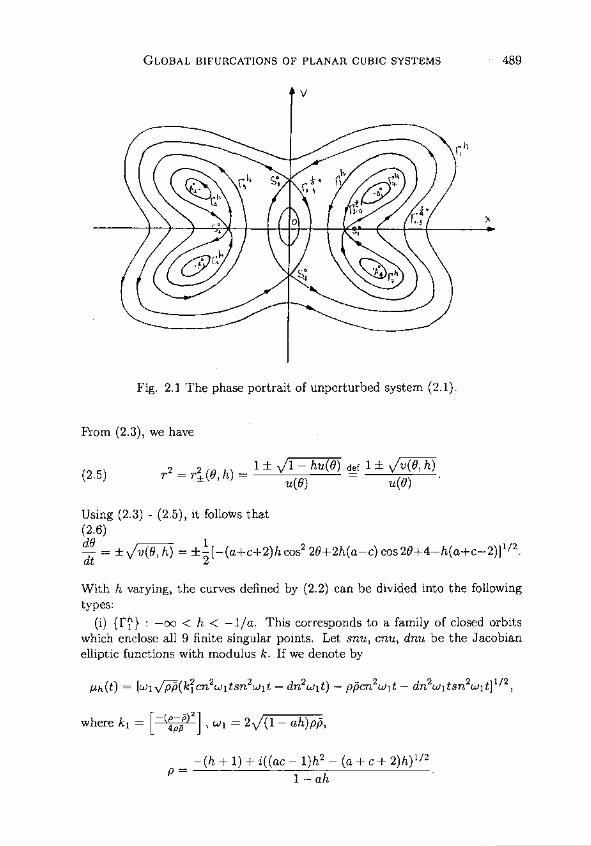
Fig . 2.1 The phase portrait of unperturbed system (2.1) .

From (2 .3), we have

GLOBAL BIFURCATIONS OF PLANAR CUBIL SYSTEMS

489

1 f

1- hu(9) def 1 t

v(0, h)(2.5)

r2 = rf (B,h) =

u(9)

-

u(9)

where k1 = [

4PP_

z] , w1 = 2V"-(-1 - ah)pp,

-(h + 1) + i((ac - 1)h2 - (a + c + 2)h) 1 /2

Using (2.3) - (2.5), it folloivs that(2.6)

= f

v(0, h) = f2 [-(a+c+2)h cos2 2B+2h(a-c) coa 2B+4-h(a+c-2)] 1/2 .

With h varying, the curves defined by (2.2) can be divided into the followingtypes :

(i) {I'1} : -oo < h < -1/a .

This corresponda to a family of closed orbitswhich enclose all 9 finite singular points . Let snu, cnu, dnu be the Jacobianelliptic functions with modulus k . If we denote by

ph(t) = [w1-,l_p_p(k2cn2W1tsn2wlt - dn 2wlt) - ppcn2W1t - dn2W1tsn2w1t]1/2,

490

J . Li, Z . Liu

Then the orbit of {I'i} has the parametric representation

-_ vhdrnwltswlt(2.7)

xl(t)

yl(t) _

cnWlt

~h(t)

Ph(t)

where -oo < h < 0.(ü) {I'2 } : 0 < h < á .

This corresponds to a family of closed curves sur-rounding the origin 0(0, 0), which has the parametric representation

(t) _~dnwltsnwlt

(t) =Pcnwlt

(2.8)

X2 (t)

y2

Ph(t)

(iii) When h = 1/a, three are 4 heteroclinic orbits connecting two criticalpoints S3 and S4 . If we let

w¡a(t) = [a(A2sh2201t f 2A1,Olch2p1t+ 1]1/2

where Ai = (a-c)/2(a+1), ,O1 = 2(a+ 1)/a, then the heteroclinic orbits r2/3+

and I'i/3+ have respectively parametric representation :

l /a+

1

-Alsh2,81t(2.9)

r23 : x2,3 (t) _ P+1/a(t)

112,3(t) -tt¡a(t) '

(210)

r13+ -13(t) -.,,wi/a(t)

hl/a(t) .

(iv) {r3±} : á < h < 1 . These are two families of closed orbits surroundingrespectively three singular points A°, S°, A4 and A2, S2, S3 . The orbit of{t3+ } has the parametric representation :

(2.11)

y3(t) = v/-h-[1 + 2aw3dn2w3tsn2w3t]-1/2acn2W3t,

where w3 = ~Q1/4 A = h[-a(ac - 1)h + (a + c + 2)], the modulo k3

a/ a2 +,Oa a2 = 1+h +./A 02 = ."A-(1+h)ah-1 ah-1

(v) When h

three are four homoclinic orbits r3/4~ surrounding respec-tively the centers A° (i = 1 - 4) and connecting respectively the saddle pointsS° and S2 . One of homoclinic orbits has the parametric representation :

(2.12)

1

A1sh2Qlty1,3(t) =

-

X3(t) =

'rh[1 + 2aW3dn2w3tsn2w3t]-1/2,

r1/C+

:x3,4(1)-

ch2,02t3,4

~[sh22Q2t + 2A2Q2sh2~32t + (1 - A2)]1/211

y3,4(t)_ .,-[sh22~2t+2A2f2sh2Q2t+(1-A2)]1/2,

GLOBAL BIFURCATIONS OF PLANAR CUBIC SYSTEMS

491

where 62 =2(1 + c) /c, A2 = 2(1 + c)/(a - c) .

(vi) {r4} : 1 < h < a~°12 . This is composed of four families of closed orbits

surrounding respectively one critical point A°(i = 1 - 4) . If we write

vh(t) = [1 + 2aw4k22sn2w4tcn2w4t + a2dn22w,t]1/2,

where w4 = [(1 + h) +

]112, k2 = (a 2 - q2)/a2, a, /p are the same as in (iv),

then one family of {rh} has the parametric representation :

N/-h- ,

Y4(t) _4adn2w4t

(2.13)

x4(t) _

.

vh(t)

Vh(t)

Note that as h increasing, the curve I'2 extends outside, the other curves con-2inside .

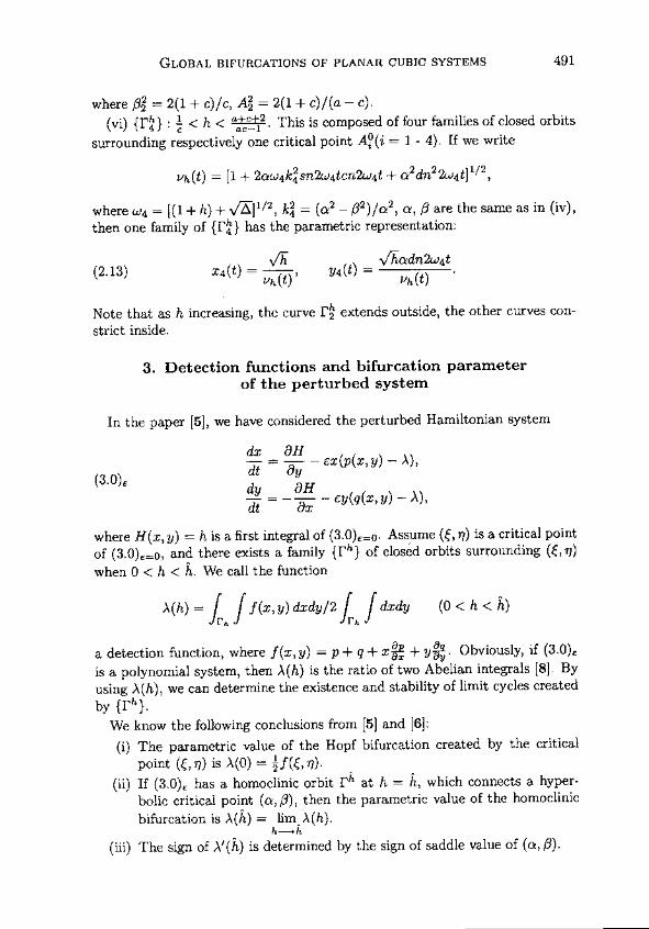
3 . Detection functions and bifurcation parameterof the perturbed system

In the paper [5], we have considered the perturbed Hamiltonian system

(3.0) Edy=

áH

d

ax - Ey(q(x, y) - ~)-

where H(x, y) = h is a first integral of (3.0),0 . Assume (1, 77) is a critical pointof (3.0),o, and there exists a family {I'h} of closéd orbits surrounding (1, 77)when 0 < h < h . We call the function

A(h) =

1 f(x, y) dxdy/2ir,f dxdy

(0 < h < h)

a detection function, where f(x, y) = 77 + q + x 2E + y?£ .. Obviously, if (3.0) Eis a polynomial system, then A(h) is the ratio of two Abelian integrals [8] . Byusing A(h), we can determine the existente and stability of limit cycles createdby {rh} .

We know the following conclusions from [5] and [6] :(i) The parametric value of the Hopf bifurcation created by the critical

point (1, 77) is A(0) = 2 f(~, ?7) .

(ii) If (3.0), has a homoclinic orbit I'h at h = h, which connects a hyper-bolic critical point then the parametric value of the homoclinicbifurcation is A(h) = lim_A(h) .

h-h

(iii) The sign of A'(h) is determined by the sign of saddle value of (a, /.i) .

492

J. Li, Z . Liu

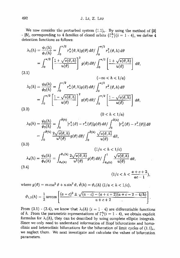
We now consider the perturbed system (1.1), By using the method of [3]- [5], corresponding to 4 families of closed orbits {rh}(i = 1 - 4), we define 4detection functions as follows :

(3 .2)(0 < h < 1/a)

A3(h)

V)3(h)=

loá(h) [r+(19) - r4 (19)lg(i%) dí%/

f~ (h) [r+(19 ) - r2 (19)) d19

(3 .3)

A1(h)

01(h) -

f

',/2 r+(i9' h)g(9) di9/J

ir/2r+ (19, h) d19

_~r/2

1 + u(19(19,

h)

2

g(19) d19/fr

l?

1 +u(19)

19, h)

d19,

(-oo < h < 1/a)

A2 (h)

02(h) -

lo

/2r4(t9, h)g(~) d19l

Jo7r/2 r2 (,0, h) di9

=

7,/2

1-

v (í9,h)

2 g(i9) d19/

7r/2

1 -

v(19, h)

d19,f [ u(19)

1

fo 1 U(79) 1

J 9(h) 2

u2~~~h) g(~) d19/

f9(h)

u(

(~)

h)d19,

(1/a < h < 1/c)

A4(h) =1G4(h) __

f,91(h) 2

2(19,h) g(i9) d19/ f 1

v(19,h) d19,

04(h)

f2 (h)

u (19)

&2(h)

u(79 )(3 .4)

where g(19) = m cos e 19 + n sin 2 19, ~(h) = ?91(h) (1/a < h < 1/c),

(1/c<h<a+c+2)ac - 1

,

1

(a-c) 2 f (a-c)-(a+c+2)(a+c-2-4/h)191,2(h) = 2 arccos I

a + c + 2

From (3.1) - (3 .4), we know that Ai(h) (i = 1 - 4) are differentiable functionsof h . From the parameterc representations of I'h(i = 1 - 4), we obtain explicitformulas for Ai(h), they can be described by using complete elliptic integrals .Since we only need to understand information of Hopf bifurcations and homo-clinic and heteroclinic bifurcations for the bifurcation of limit cycles of (1.1) E ,we neglect them . We next investigate and calculate the values of bifurcationparameters .

(3.6)


493

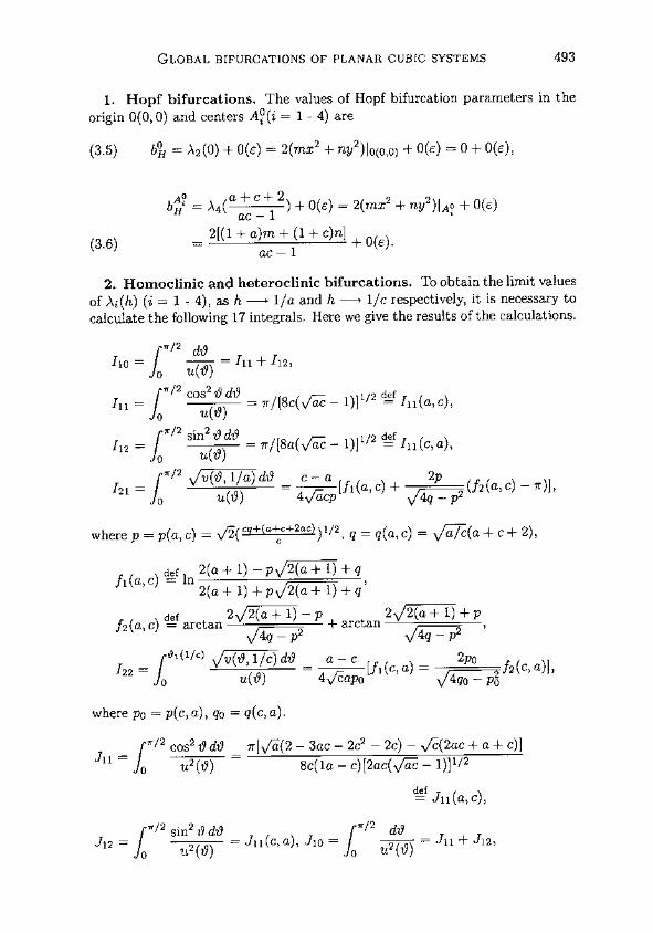
1 . Hopf bifurcations. The values of Hopf bifurcation parameters in theorigin 0(0, 0) and centers A°(i = 1 - 4) are

(3.5)

bol = 1\2(0) + 0(e) = 2(mx2 + ny2) 10(0,0) + 0(s) = 0 + 0(s),

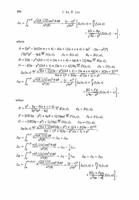
2 . Homoclinic and heteroclinic bifurcations . To obtain the limit valuesof Aj(h) (i = 1 - 4), as h --> 1/a and h -+ 1/c respectively, it is necessary tocalculate the following 17 integrals . Here we give the results of the calculations .

a+c+2ac - 1 ) + 0(e) = 2(mxz + ny 2 )I a~ + 0(E)

- 2[(1 + a)m + (1 + c)n] + 0(s) .ac - 1

,lo =

) = Ill + 112,o u

I11 - ~f71/2 cou(~>19=7r/[8c(~- j),1/2 del I11(a,c) ,

112 = f"/z siu(19

)

= 7r/[8a(~- 1)] 1/2 delI11(c, a),

0/2

v(19, 1/a) d19 =

c- a

2pIzl =

lo"

u(19)

4~cp [fl (a, c) +

4q-

pz(f2 (a, c) - ~)]

where p = p(a, c) = "/2( eg+(d+c+2dc) )1/2

q = q(a c) =

a/c(a + c + 2),

1(a c) def ln 2(a + 1) - p

2(a + 1) + qf 2(a + 1) + p

2(a + 1) + q

def

2

2(a + 1) - p

2

2(a + 1) + pf2 (a, c) = arctan

+ arctan

,4q - p2

4q - p2

~'(1/e)

v(í9,1/c) d19

a - c

2poIzz =r

u(19)

=4~apo

[f1(c, a) =

4qo - p2ofz(c

where po = p(c, a), qo = q(c, a) .

/2 cos2 í9 d19 _ 7r[_f (2 - 3ac - 2c 2 - 2c) - f(2ac + a + c)]J11

_- fo

~

u2 (19)

8c(1a - c)[2ac(~- 1)] 1/20

defJ11(a, C),

n/2 sin2 19 d19

~/2

d19J12 =

f

u2 (19)

= J11(c, a), J1o = f

u2(1%)

= J11 + J12,19)

a)],

494

J . Li, Z . Liu

7r /z

v(19, 1/a) cos2 19 d19

(c -a 2

BJ21 = fo

uz (19)

_

,~ a-c2[fo1(a,c) + 2f1 (a, c)C2

A = [(p2 - 2q)(3a + c + 4) - 4(a + 1)(a + c + 2) + 2q2 - (2q - p2)2]/[2p2 (p2 - 4q)]

def A(ac),

Ao = A(c, a),

BO =B(c, a),B = [(2q -pz)(2A + 1) + (3a + c+ 4) + 4q(A + 1)]/8pq dof

B(a, c),D = -[(2q - pz ) (2A + 1) + (3a+ c+ 4)]/8q

de fD(a, c),

Do=D(c, a),

fo1(a, c) def

2(a_

_+1)[(2q - p2 ) (2A+ 1) + (3a + c+ 4)]/4 -F- A(2a + 2)3/24(a + 1)2 + 2(2q - p2) (a + 1) + qz

'~/2

v(19,1/a) sin2 í9 d19

(c - a)2

FJz2 =f

u2 (19)

_

~c2[f~2(a, c) + 2f1(a, c)

+ 2G+Fp

4q--p2(f2 (a, c) - 7r)

J,

where

2p2(p2 - 4q)

E(a, c),

Eo

E(c, a),

F = [2E(2q -p2) + 4qE + 1]/(8pq) def F(a, c),

Fo = F(c, a),G = -[2E(2q - p2) + 1]l(8q)

def G(ac),

Go =G(c, a),def

2(a + 1) [2E(2q - p2 ) + 1]/4 + E(2a + 2)3/2foz (a, c) =

4(a + 1)2 + 2(2q - p2) (a + 1) + q2'~/z

v(19, 1/a) d19J2o =f

u2(119)

= J21 + Jzz,

~/2 v(i9,1/a) COS219 d19

1J31 = fo

u2(1%)

=Jii -a Iii,

~/2 v(19,1/a) sin 2 19 d19

1J3z =

u2(19)

= Jiz -a

I12,

Jso = J3 1 + J3z,~

0

J41 =

d'(1/°)

v(19,1/c) cosz 19 d19 - (a - c)zlo

u2 (19 ) 11/C--a2

+ 2D+ Bp

4q- p2 (fz(a, c) -

I ,

1f02 (c,a)+ 2o f1 (c, a)

+2Go + Fopo

fz (c,a)J

,4qo - po


495

191(1/C)

v(j, 1/c) sin2 19 d19 - (a_ c)2

BoJ42 =fu2 (1_9)

ca2

[fo1(c,a) + 2fl(c,a)0

X1 (1/C)

v(19, 1/c) dl9J40 =

,a2 (19 = J41 + J42 .o

Using (3.1) - (3.4) and the previous integrals, we have

(3.7)

(3.8)

(3.9)

(3.10)

2Do + Bopo+

f2(c,a)I ,49o - po

1

_ m_(J11+2J21+J31)+n(J12+2J22+J32)1 (a)

I1o+121

A21 m(Jll - 2J21+J31)+n(J12+ 2J22 + J32)

Ca/=

I10 - 121

As

1

_ 2(mj2l + nJ22)Cal

121 ,

A3

1

-A4

(1) - 2(mJ41 + nJ42)c c

122

Note that A ;, (Q) and Aj(i= 1 - 3, j = 3,4) give respectively the parametervalues of heteroclinic and homoclinic bifurcations .

Proposition 3.1 .

if Al

> A2

than A3

> Al'(

> A2

IfAl~~~ <A2a

, thanA3~~~ GAIa

<A2~a ~ .

Proof.. From (3 .1) - (3.4), we know that

(3.11)

Al ( 1

_ A2 ( 1

__ V)l(1_

_

/a)02(1/a) - 02(1/a)01(1/a),a a 01(1/a)02(1/a)

and

(3.12)

A3 (1) - Ai (1) -_ 11( 1/a)02(1/a) - 02( 1/a)01(1 /a) i = 1,2 .a

a

Oi( 1/a)[01( 1/a) - 02(1/a)]

It is easy to see that

03

_ 01 ~ a ~ - 02 ~a ~ > 0,

0¡(~)

> 0

(i = 1, 2) .

Thus, (3.11) and (3.12) gives the conclusion .

496

J . Li, Z . Liu

3 . The values of saddle points Sj - the detection values of direction of homo-clinic and heteroclinic bifurcations . Under the condition that the unperturbedvector field has some symmetries, the sign of the values of a saddle point can beused to determine the stability of a bifurcating closed orbit from a homoclinicor heteroclinic loop, and give the signs of Ai(1/a), Aí (1/c) (á = 1, 2, 3, j = 3,4) .At the saddle points S1 and 52, when the parameter A talces the values of

Aj (1/c) (j = 3, 4), we have

(3.13)

By using (3 .7) - (3 .9), we obtain

Hence, from 3, we have

U3 , 4 = 2E[2(mx2 + ny2)¡s, - A3 (1/c)] + 0(E2)- 4E

rrn(I22 - cJ41) - nCJ42

+ 0(E2) .Ill..

cI22

Similarly, at the saddle points S3 and S4, when A = Ai(1/a) (i = 1, 2, 3), wehave

al = 2E[2(mx2 + ny2 )I S3 - Ai(1/a)] +0(,52) .

(3.14)[2(110 + 121) - a(J12 + 2J22 + J32)]n - ma(J11 + 2J21 + J31) + 0(E2) ;al = 2E

a(11o + 121)(3.15)

a2 = 2E [2(110 - 121) - a(J12 - 2J22 + J32)In - ma(J11 - 2J21 + J31) + 0(E2) .a(I1o - 121)

,(3.14)a3 = 4e (12 1 - aJ22)n - amJ21 +

0(E2) .aI21

4 . Global and local bifurcations in the cases m = n

If we let m = n, then (1.1) becomes

dx_ =y(1 + x2 - ay2 ) + Ex(mx2 + my2

dt

d =-x(1

-CX2 + y2) + Ey(mx2 + my2

X1 (1) = m(J1o + 2J2o + J3o)

A2(1) = m(J1o - 2J2o + J3o)

a

110 + 121

a

110 - 121

A31

_ 2mJ2o

A41

- 2mJ4oCa/ 121 '

(c) 122

A _ 2m(a + c + 2)

o


497

Lemma 4.1 . A'3 (h) > 0, V4(h) > 0 and

lim

\'3(h) = +oo,h-1/a+0

lim

As(h) =

lim

A4(h) = +oo.h-1/c-0 h--11/c+0

Proof.- Since

we see from (3.4) that

I defV)303 - 03w3

1

9i1

-

(h)_

d19

91 (h)

~d19 -

~ 1(h)

d19

`91 (h)

~d29~ ~ 22

19,1 (h) UV~

-V

,91

v(h)

26

J-,9 1 (h) V J-,9 1(h)1-,

u

This integral formula can be written as a double integral [4] :

d_ef

~1(h)

~1(h)

[21,1(191) _ u2(192)](4.2)

I - ~

4191 d192 > 0 .'91 (hl -~1(h) ui(~%1)uá(~%2) v1v2

When h tends to 1/a or 1/c, at 19 = 0 of 19 = 7r/2, the function [v(19, h)] -112 isunbounded . From (4.2), this implies that

lim

\'3 (h) =

lim

\3 (h) =+oo.h-~1/a+0 h-+1/c-0

Similarly, we can Nave the result for V4(h) . Lemma 4.1 implies that Q3,4 <

O, Q3<0.

Lemma 4.2 .

d ( ~~ (h ) < 0 d (~h_) ) < 0.dh ~i(h)

~ dh ~z(h)

Proof.For i = 1, 2, we have

Using (3.1) and (3 .2), we know that

.Idef

~i~(h)~i(h) - 0z~(h)Oz(h)

_~1 ~ rn/2 d19

n12 d19 -

~12 d19

n12ud19

w12 d19

n12 ud19

4 J0

~ o

v3/2

o

u~ o

v3/2 + o

u

o

v3/2

(4.3)2

3/22

d9 d9 I/.1 1 1 2 .vlv2 3/2

1 +

v1

.

1 +

v2

7r/2

7,2

1

vil +_

v1v2

v2+ v1v

The signs - and + on the right hand of, (4 .3) are respectively corresponding tothe cases of i = 1 and i = 2. Thus, (4.3) gives the conclusion of Lemma 4.2 .

498

J . Li, Z . Liu

Lemma 4.3 . [5] For h E (0, ho), assume that the functions O(h) and 1P(h)are suficiently smooth, nonnegative and monotone increasing, the functionV)'(h)l0'(h) is nonnegative and monotone increasing (decreasing) . Then thefunction O(h)/o(h) must satisfy one of the following propertáes :

(i) monotone increasing after it decreases to a minimum (monotone de-creasing after it increases to a maximum);

(ii) monotone increasing;(iii) monotone decreasing.

In particular, if 0(0) = 0(0) = 0 and tilim0O(h)/0(h) = a > 0 (or < 0), then

V)(h)l0(h) must be increasing (decreasing) .

Lemma 4.4 .

lim A1(h) =+oo .h-+-oo

Proof. Write r~ = min,oE [o z,,) r+(1%, h), h E (-oo, 0), because I'i extendsinfinitely as h , -oo, it fóllows that rz ,+oo, as h -> -oo. We have

lim

A1 (h) >

lim

(rñ1

r+ d~9/

r+ d19) =

lim

rá = +ooh--oo

-h-.-oo

0

0

h--oo

Lemma 4.5 . If A1 (á) > á, then Al(h) will be monotone increasing afterit decreases to a minimum; if A1 (d) < á, then Al(h) is monotone decreasing,and A2(h) is monotone increasing .

Proof.. If A1 (-1) > m, then ul < 0, Le .,

lim

Al(1/a) = +oo. Thus,h-1/a-o

Lemma 4.2 - 4.4 can follow the first part of the conclusion of Lemma 4.5 . Onthe other hand, 0z(0 ) = 0z(0) = 0, Lemma 4.2 and Lemma 4.3 lead to theresult stated for \' (h) a

Lemma 4.6 . For the system (4.1) E , the inequality A3 (á) > Al (á) > .1z (d)holds.

Proof. We have

A1

1

-Az

(1) = 2(1o + J3o)Jll + 4JzoJlo > 0a a Izoz-Iz11

by using Proposition 3 .1, we have Lemma 4.6

These lemmas enable us to determine two types of detection curves of (4.3) E ,shown as Fig . 4.1 (a) (b) .


499

Proof.. From (3.1), we have

n~2 1+ vf, h) 2

V)1(h) =

u(19)

1

g(0) d19

(a)

(b)

If ~1 ~ -ai ) > ~,

If \ 1 ( «a) <

Fig . 4.1 The detection curves of (1.1), when m = n.

5 . Bifurcation set in the (n, m) plane

We now consider the general case of m :~ n for the system (1 .1),

Lemma 5.1 .hlim

A1 (h) = +oo, if m+ k, (á,c)n > 0;h

lim

A1 (h) _

-oo, if m + kl(a, c)n < 0, where kl(a, c) = I121III

- 2

~i2gA d19 + 2

wi2

v(19' h) g(19) d19 - hJ

~/2g(~) dí9

o u2 (19) o u2 (19)

o u(19)

. . .)+( . . .)-hIll(m+kl(a,c)n) .

Since 01 (h) is exactly a quarter of the area insider I'i , we have 01(h) - +ooas h - +oo . Clearly, as h --> -oo, the sign of lim A1(h) is determined bythe third term of (5.1) . Hence, Lemma 5.1 is true .

500

J . Li, Z . Liu

Next, we apply the results of 3 to partition the parameter plane (n, m) asregions of angles, inside which there are different detection curves of (1.1),Without loss of the generality, we only discuss the case of m _> 0 . In the upperhalf plane of (n, m), we have 18 half straight lines with linear equations asfollows .

1 . The line 11 is use to distinguish the sign of

lim

A1(h) .h-.-oo

(5.2)

11 : m = -k1 (a, c)n,

k,(a, c) = 112/hl-

15 : Q3,4 = 0, m =

cJ42

n = k5 (a, c)n .[122 - CJ41 1

3 . Straight lines 16 - 113 determine the relations between Hopf bifurcationparameters and homoclinic, heteroclinic bifurcation parameters .

(i) al(1/a) = 6,

[ J12+2J22+J32 1 __(5.7)

16 : m = -

Jll + 2J21 + J31

n

ks(a, c)rt,

(ii) A2 (1/a) = 0,

_

[

J12 -2J22+J32 1

(iii) A3(1/a) = 0,

l(5.9)

lg : m = -

J2z(J22

n__

k8(a, c)n ;

2 .to

Straightzero .

lines 12 - 15 show that values of saddle points of (1.1), are equal

(5.3)2(Ilo +121)-a(J12+2J22+J32) 1

12 :0'1 =0, m=1

=a(J11+2J21+J31)

n k2 (a, c)n;

(5.4)2(Ilo - 121) - a(J12 - 2J22+J32) 113 :0'2 =0, m=

1=

a(J11+2J21+J31)n k3 (a, c)n;

(5 .5)121 - aJ22 __

(5 .6)

(iv) \ 4 (1/c) = 0,

(5.10)

(5.14)

(5.15)


501

(v) bH - A1(1 /a) = 0,(5.11)

_

2(1 + c)(I1o + 121)l10

m

- 12(1 +a)(Ilo+121)

(vi) bA? - A2(1/a) = 0,(5.12)

111 :m=_ 2(1 + c)(Ilo - 121)[2(1 + a)(Ilo - 121)

(vi¡) bA - .1,(l/a) = 0,

(viii) bg0- A,(1/a) = 0,

(i) a1(1/a) - .\3(1/C) = 0,

(ii) ñ1(1/a) - \4(1/c) = 0,

(iii) A2(1/a) - A4(1/c) = 0,

(ac - 1) (J1 2 + 2J22 + J32) n = k1o(a, c)n ;(ac - 1)(J11+2J21+J31)]

(ac-1)(J12-2J22+ J32) ] n=(aC - 1)(J11 - 2J21 + J31)

(5.13) 112 :rn=-[(1+a)I21-(ac-1)J21]n_k12(a,c)n ;

_

(1 + c)122 - (ac - 1) J42

__113 .m_-[(1+a)722-(ac-1)J41] k13(a,c)n;

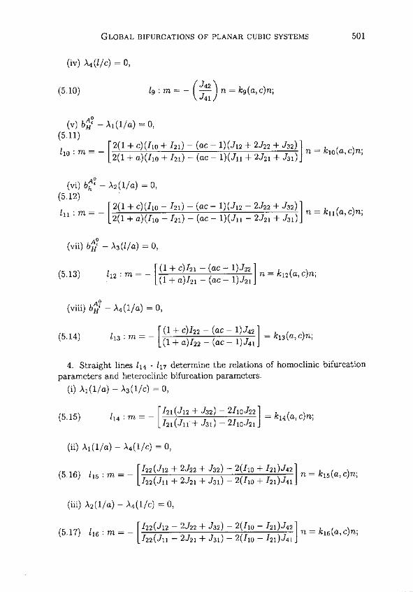
4 . Straight lines 1 14 - 1,7 determine the relations of homoclinic bifurcationparameters and heteroclinic bifurcation parameters .

121(J12+J32) - 211oJ22 __[12,(J11+J31) - 21,oJ21]

k,

(a, c)n ;

(5.16)

115 : m

122(J12 + 2J22 + J32) - 2(I1o + 121) J42= -

n= k1s(a, c)n ;[I22(Jll+2J21+J31) - 2(I10+I21)J41

rI22(J12 - 2J22 + J32) - 2(I1o - I21)J42 ](5 .17)

l1s : m = -

n= k1s(a, c)n ;122(J11-2J21+J31) - 2(Iio - I21)J41

502

J . Li, Z . Liu

(iv) A3(1/a) - A4(1/c) = 0,

_(5.18)

117

m=

fI22J22-I21J42 n _k17(a, c)n .122J21 - 122 J41 1

5 . The straight line 1,s determines the relation between Hopf bifurcation0

parameters, Le . bH' - bo = 0.

(5.19)

11s : m = - (1 + a)n

kl8(a, c) n.

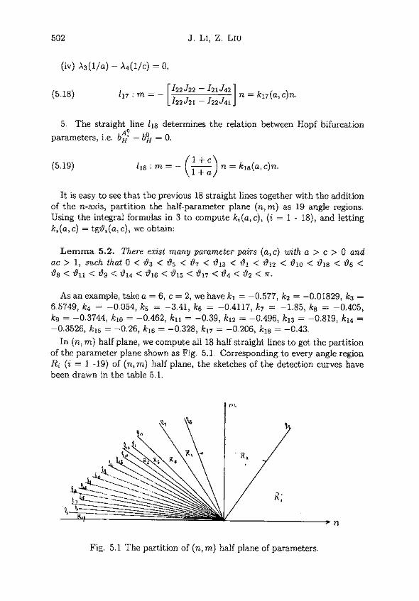
It is easy to see that the previous 18 straight lines together with the additionof the n-axis, partition the half-parameter plane (n, m) as 19 angle regions .Using the integral formulas in 3 to compute k¡ (a, e), (i = 1 - 18), and lettingki (a, c) = tg19i (a, c), we obtain :

Lemma 5.2 . There exist many parameter pairs (a, c) with a > c > 0 andac> 1, suchthat0<193<195<197<1913<191<1912 <1910<1918<296<198<1911 <199<1914<2916<1915 <1917<794<292GIr-

As an example, take a = 6, c = 2, we have k1 = -0.577, k2 = -0.01829, k3 =6.5749, k4 = -0.054, k5 = -3.41, k6 = -0.4117, k7 = -1 .85, k8 = -0.405,k9 = -0.3744, klo = -0.462, k11 = -0.39, k12 = -0.496, k13 = -0.819, k14 =-0 .3526, k15 = -0.26, k16 = -0.328, k17 = -0 .206, kis = -0.43.In (n, m) half plane, we compute all 18 half straight lines to get the partition

of the parameter plane shown as Fig . 5 .1 . Corresponding to every angle regionRi (i = 1 -19) of (n, m) half plane, the sketches of the detection curves havebeen drawn in the table 5.1 .

Fig . 5 .1 The partition of (n, m) half plane of parameters .


503

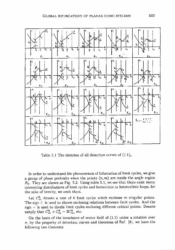
Table 5.1 The sketches of all detection curves of (l.l),

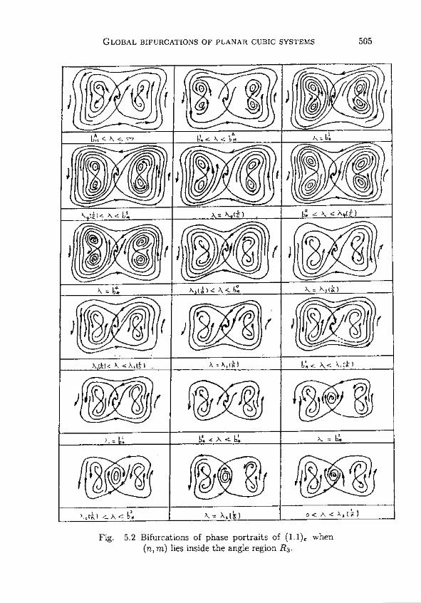
In order to understand the phenomenon of bifurcation of limit cycles, we give

a group of phase portraits when the points (n, m) are inside the angle region

R3 . They are shown as Fig . 5 .2 . Using table 5.1, we see that there exist many

interesting distributions of limit cycles and homoclinic or heteroclinic loops, for

the sake of brevity, we omit them.

Let C.,denote a nest of k limit cycles which encloses m singular points .

The sign C is used to shown enclosing relations between limit cycles . And the

sign + is used to divide limit cycles enclosing different critical points . Denote

simply that C. + Ck,,, = 2Ck,,,, etc .

On the basis of the invariance of vector field of (1.1) under a rotation over

7r, by the property of detection curves and theorems of Ref. [5], we have the

following two theorems.

6h a ~a

A

I4

^L

,

ói ÚR 1 6N 11

á L h~ h a C . h P C I ,. h , 1 . ,GA ho~I

(i . K

1

h'

k

h h.

a h~. . ¿ hu '~) 11,11~i

Lnh, It

Rs R R K R�

iL

l~ILI, 'Iklk

hL

lí

h

R �

H

R, Z Rrn R ..

M

R.f

k-¡ h.-_;c _ i_\. . h

4VI

I l,,i

6Ñ -

R~E ~~76H R

~ w 'R~Y

504

J . Li, Z. Liu

Theorem 5.1 . For any fixed e, 0 < e << 1, when (n, m) is inside the angleregion R3 of Fig. 5.1, as A varies, (1 .1). has distributions of limit cycles andhomoclinic or heteroclinic loops as follows:

(i) If bH < A < +oo, (1 .1), has one unstable limit cycle with the distributionC9 .

(ü) If b; < A < bH, (1.1). has 5limit cycles with the distribution of C9 D 4Ci .

(iii) If A = b3, (1 .1)E has 7 limit cycles with the distribution of C9 D 2[C3 D2Ci ] .

(iv) If A4(1/c) < A < b;, (a.a)E has 9 limit cycles with the distribution ofC9 D 2[C3 D 2Ci] .

(v) If A = A4(1/c), (1 .1), has !, homoclinic loops connecting respectively thepoints Sl and S2, with the addition of 7 limit cycles .

(vi) If b* < A < A4(1 /c), (1 .1). has 11 limit cycles with the distribution ofC9 D 2[C3 D 2C2] .

(vi¡) If A = b*, (1 .1)E has 7 limit cycles with the distribution of C9 D 2[C3 D2C'].

(viü) If A3(1/a) < A < b*, (1.1), has 3 limit cycles with the distribution ofC9 D 2C3' .

(ix) If .1 = A3 (1/a), (1 .1)E has 2 homoclinic loops connecting respectively thepoints S3 and S4, with the addition of one limit cycle C9 .

(x) If A = A1(1/a), (1 .1)E has two heteroclinic loops which are surroundingrespectively 3 critical points; outside there loops, there is one limit cycle C9 .

By using Table 5.1, we also see that the following result is true .

Theorem 5 .2 . For afixed e, 0 < e << 1, we have

(i) If (n, m) is inside the angle region R12, then the distributions of limitcycles of (1 .1), are

(a) 7limit cycles with 2[C3 D 2C'] +C' distribution, when .\3(1/a) < A < 0;

(b) 6 limit cycles with C9 D 5Ci distribution, when \2(1/a) < A < A1(1/a);

(c) 4 limits cycles with 2Cs distribution, when A4(1/c) < A < b; .

(ii) If (n, m) is inside the angle region Rlo, then there are 5 limit cycles of(1.1), with the distribution 5Ci, when A1(1/a) < A < 0. This is the Il'jasenkodistribution .


505

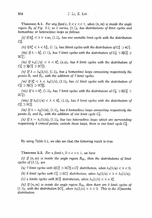
Fig .

5.2 Bifurcations of phase portraits of (1.1), when(n, m) lies inside the angle region R3.

oj oP

~~ ~ o

r

o 0

_~I~

ph

I~Q

f O~ OD1O

o ~r J ~ r i

J( ~~ ~ ~- r r ) r

J

0 1wsg

506

J. Li, Z . Liu

Referentes

1 .

V.I. ARNOLD, "Geometric methods in Theory of ordinary differential equa-tions," Springer-Verlag, New York, 1983 .

2 .

LI JIBIN, Researches on the weakened Hilbert's 16th problem, Journal ofKunming Institute of Technology 13 (1988), 94-109 .

3 .

Li JIBIN ETC., Bifurcations of limit cycles forming compound eyes in thecubic system, Chin . Ann. of Math . 8B (1987), 391-403 .

4 .

A.I. NEISTADT, Bifurcations of phase portraits for some equations ofstability loss problem at resonante, Appl . Math . and Mech . 42 (1978),830-840, (in Russian) .

5 .

LI JIBIN ETC., Planar cubic Hamiltonian systems and distributions of limitcycles of (E3), Acta Math . Sinica 28 (1985), 509-521 .

6 .

Lf JIBIN ETC., Global Bifurcations and chaotic behaviour in a disturbedquadratic system with two centers, Acta Math . Appl . Sinica 11 (1988),312-323-

7 .

JU . S . IL'JASENKO, The origin of limit cycles under perturbation of theequation dw/dz = -RZ/R, where R(z, w) is a polynomial, Math . Sbornik78 (1969), 360-373 .

8 .

J . CARR, S.N . CHOLA AND J.K . HALE, Abelian integrals and bifurcationtheory, Journal of Differential Equations 59 (1985), 413-437.

Jibin Li : Center for Dynamical Systems and Nonlinear StudiesSchool of MathematicsGeorgia Institute of TechnologyAtlanta, GA 30332U.S.A .

Zhenrong Liu: Department of MathematicsYunnan University650091 YunnanP.R . CHINA

Rebut el 21 de Desembre de 1990

bifurcation setandlimitcycles...

Documents