journal of sound and vibration - uni-stuttgart.de

Journal of Sound and Vibration 501 (2021) 116043

Contents lists available at ScienceDirect

Journal of Sound and Vibration

journal homepage: www.elsevier.com/locate/jsv

A complete set of design rules for a vibro-impact NES based

on a multiple scales approximation of a nonlinear mode

Balkis Youssef ∗, Remco I. Leine

Institute for Nonlinear Mechanics, University of Stuttgart, Germany

a r t i c l e i n f o

Article history:

Received 1 October 2020

Revised 11 February 2021

Accepted 21 February 2021

Available online 22 February 2021

Keywords:

Nonlinear energy sink

Backbone curve

Free decay

Targeted energy transfer

Slow invariant manifold

a b s t r a c t

The aim of the paper is to formulate a complete set of design rules for a vibro-impact

nonlinear energy sink (VI NES). Hereto, analytical and numerical methods to extract the

backbone curve of vibro-impact systems are presented. The adopted approach exploits the

multiple scales method and is applied to a linear oscillator coupled with a VI NES. The

dynamics of the system are explored and the system’s response under harmonic forcing in

the vicinity of resonance is analyzed and approximated. The presented method allows for

the derivation of a closed-form approximation of a nonlinear mode. The relation between

the steady state response and the input parameters is established. The resonance frequency

of the examined nonlinear system for different excitation levels is estimated and the corre-

sponding backbone curve is identified. The theoretical predictions are confirmed through a

comparison with the standard resonant decay method combined with a phase-locked loop.

Finally, the closed-form approximations are used to derive a complete set of design rules

for a vibro-impact nonlinear energy sink.

© 2021 The Authors. Published by Elsevier Ltd.

This is an open access article under the CC BY-NC-ND license

( http://creativecommons.org/licenses/by-nc-nd/4.0/ )

1. Introduction

The present paper gives a closed-form expression for the backbone curve of 1:1 internal resonance with 2 symmetric

impacts per period of a single DOF oscillator with vibro-impact nonlinear energy sink. Based on these results, a complete

set of closed-form design rules for a vibro-impact nonlinear energy sink are derived.

A nonlinear energy sink (NES) is a technique for passively reducing vibration amplitudes and/or decay of structures [28] .

A NES consists of an auxiliary mass which is attached to the primary structure by using e.g. a nonlinear spring, similar to a

tuned vibration absorber. However, unlike a tuned vibration absorber, the working principle of a NES relies on irreversible

energy pumping from the primary structure into the NES, also known as targeted energy transfer (TET) [10,20,28] . A NES

has usually no inherent natural frequency and is able to absorb energy over a wide range of frequencies. Different types of

coupling between the primary structure and the auxiliary mass have been studied theoretically [1,2,13,16,17] and experimen-

tally [6,14,15,21,22] in order to understand the essential changes caused by such a coupling. Many studies (e.g. [3,13] ) have

been conducted to understand the working principle of NES, being strongly related to the theory of nonlinear modes (NM).

Different numerical approaches, including control-based methods (e.g. [23,25] ), have been applied to approximate NMs of

∗ Corresponding author.

E-mail addresses: [email protected] (B. Youssef), [email protected] (R.I. Leine).

https://doi.org/10.1016/j.jsv.2021.116043

0022-460X/© 2021 The Authors. Published by Elsevier Ltd. This is an open access article under the CC BY-NC-ND license

( http://creativecommons.org/licenses/by-nc-nd/4.0/ )


http://www.ScienceDirect.com

http://www.elsevier.com/locate/jsv

http://crossmark.crossref.org/dialog/?doi=10.1016/j.jsv.2021.116043&domain=pdf

http://creativecommons.org/licenses/by-nc-nd/4.0/

mailto:[email protected]

mailto:[email protected]


http://creativecommons.org/licenses/by-nc-nd/4.0/

B. Youssef and R.I. Leine Journal of Sound and Vibration 501 (2021) 116043

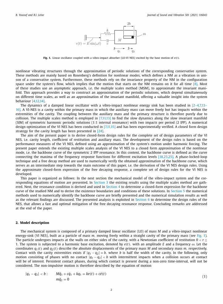
Fig. 1. Linear oscillator coupled with a vibro-impact absorber (LO-VI NES) excited by the base motion of e (t) .

nonlinear vibrating structures through the approximation of periodic solutions of the corresponding conservative system.

These methods are mainly based on Rosenberg’s definition for nonlinear modes, which defines a NM as a vibration in uni-

son of a conservative system. Furthermore, these methods rely on the invariance property of the NM in the configuration

space under the system’s flow, which implies that the motion that starts on the NM remains on it for all time [8] . Most

of these studies use an asymptotic approach, i.e. the multiple scales method (MSM), to approximate the invariant mani-

fold. This approach provides a way to construct an approximation of the periodic solutions, which depend simultaneously

on different time scales, as well as an approximation of the invariant manifold, offering a valuable insight into the system

behaviour [4,12,14] .

The dynamics of a damped linear oscillator with a vibro-impact nonlinear energy sink has been studied in [2–4,7,13–

16] . A VI-NES is a cavity within the primary mass in which the auxiliary mass can move freely but has impacts within the

extremities of the cavity. The coupling between the auxiliary mass and the primary structure is therefore purely due to

collision. The multiple scales method is employed in [7,11,13] to find the slow dynamics along the slow invariant manifold

(SIM) of symmetric harmonic periodic solutions (1:1 internal resonance) with two impacts per period (2 IPP). A numerical

design optimization of the VI NES has been conducted in [7,11,15] and has been experimentally verified. A closed form design

strategy for the cavity length has been presented in [24] .

The aim of the present paper is to derive closed-form design rules for the complete set of design parameters of the VI

NES, i.e. cavity length, coefficient of restitution and auxiliary mass. The development of the design rules is based on the

performance measures of the VI NES, defined using an approximation of the system’s motion under harmonic forcing. The

present paper extends the existing multiple scales analysis of the VI NES to a closed form approximation of the nonlinear

mode, i.e. the backbone curve of the symmetric 2 IPP resonance. In this context, the backbone curve is defined as the curve

connecting the maxima of the frequency response functions for different excitation levels [18,23,25] . A phase-locked-loop

technique and a free decay method are used to numerically verify the obtained approximation of the backbone curve, which

serves as an intermediate step towards the main outcome of this paper, i.e. the derivation of the VI NES design rules. Using

the approximate closed-form expression of the free decaying response, a complete set of design rules for the VI NES is

developed.

This paper is organized as follows: In the next section the mechanical model of the vibro-impact system and the cor-

responding equations of motion are presented. In Section 3 the existing results using the multiple scales method are gath-

ered. Next, the resonance condition is derived and used in Section 4 to determine a closed-form expression for the backbone

curve of the studied NM and to derive the existence boundaries and conditions of these solutions. In Section 5 the numerical

methods used to numerically identify the backbone curve are briefly presented and the numerical simulation results as well

as the relevant findings are discussed. The presented analysis is exploited in Section 6 to determine the design rules of the

NES, that allows a fast and optimal mitigation of the free decaying resonance response. Concluding remarks are addressed

at the end of the paper.

2. Model description

The mechanical system is composed of a primary damped linear oscillator (LO) of mass M and a vibro-impact nonlinear

energy-sink (VI NES), built as a particle of mass m, moving freely within a straight cavity of the primary mass (see Fig. 1 ).

The particle undergoes impacts at the walls on either sides of the cavity, with a Newtonian coefficient of restitution 0 < r ≤1 . The system is subjected to a harmonic base excitation, denoted by e (t) , with an amplitude E and a frequency ω. Let the

coordinates q 1 ( t ) and q 2 ( t ) describe the absolute displacements of the primary mass M and secondary mass m, respectively.

Contact with the cavity extremities exists if | q 1 − q 2 | = b, where b is half the width of the cavity. In the following, only

motion consisting of phases with no contact | q 1 − q 2 | < b with intermittent impacts when a collision occurs at contact

will be of interest. Persistent contact phases, during which contact is present during a non-zero time-interval, will not be

considered. The non-impulsive motion is therefore described by the equation of motion

| q 1 − q 2 | < b : M ̈q 1 + c ̇ q 1 + kq 1 = ke (t) + c ̇ e (t)

m ̈q 2 = 0

(1)

2


where k and c represent the stiffness and damping coefficients of the LO. The impulsive dynamics is governed by the New-

tonian impact law and the conservation of linear momentum:

| q 1 − q 2 | = b : (

˙ q + 1

− ˙ q + 2

)= −r

(˙ q −1

− ˙ q −2

)M ̇

q + 1

+ m ̇

q + 2

= M ̇

q −1

+ m ̇

q −2

(2)

The superscripts (·) − and (·) + denote the value at the time instant immediately before and after the impact, respectively,

and a dot above a variable represents the differentiation with respect to time t .

Following [5,13,26,27] , the equations of motion (1) and (2) are transformed in a normalised form, which allows the

response analysis to be performed in a general framework. The transformation starts with a nondimensionalization of the

system variables and parameters, followed by a transformation of the coordinates. For this purpose, the following normalised

parameters are introduced

ε =

m

M

, ˜ E =

E

b , G =

˜ E

ε, ω 0 =

√

k

M

, � =

ω

ω 0

, λ =

c

mω 0

. (3)

The displacements q 1 and q 2 are made dimensionless by using the cavity length parameter b as a characteristic distance.

˜ q 1 =

q 1 b

, ˜ q 2 =

q 2 b

. (4)

Moreover, the time variable t is scaled by the undamped natural frequency ω 0 , leading to the dimensionless time

τ = ω 0 t . (5)

Next, barycentric coordinates v and w that represent the displacement of the center of the mass and the internal displace-

ment of the NES, respectively, are introduced as follows:

v =

˜ q 1 + ε ˜ q 2 , w =

˜ q 1 − ˜ q 2 . (6)

Substituting (6) in (1) and (2) along with a harmonic base excitation function e (t) = E sin (ωt) yields the following trans-

formed equations of motion:

| w | < 1 : v ′′ +

ελ

1 + ε(v ′ + εw

′ ) +

1

1 + ε(v + εw ) = εG sin (�τ ) + ε2 �λG cos (�τ )

w

′′ +

ελ

1 + ε(v ′ + εw

′ ) +

1

1 + ε(v + εw ) = εG sin (�τ ) + ε2 �λG cos (�τ )

(7)

| w | = 1 : v + = v − , v ′ + = v ′−

w

+ = w

− , w

′ + = −rw

′− (8)

where the prime symbol (·) ′ represents the differentiation w.r.t. the dimensionless time τ . The dynamics described by

Eq. (7) look similar and result from substituting (6) in (1) , delivering

˜ q ′′ 2 = 0 ⇒ v ′′ − w

′′ = 0 ⇒ v ′′ = w

′′ . (9)

The presence of impacts renders the system nonsmooth and therefore strongly nonlinear. Near the primary resonance ( ω �

ω 0 ) the steady state response is expected to be periodic. Of engineering interest is the periodic response of the system for

small values of the mass ratio ε, which will be taken as perturbation parameter.

3. Multiple scales method

In this section the existing results [2–4,7,11,13,16] for the VI-NES using the multiple scales method are gathered and the

steady-state response and its stability are analyzed in Section 3.2 . The first step in the analysis of the model described by

(7) and (8) requires the approximation of the solutions, whereby the corresponding quantities are uniformly expanded in

power series of a small parameter. In this context, the mass ratio ε is used as a perturbation parameter to define the new

time scales necessary to carry out the analysis using the multiple scales method (MSM) [19] . The multiple scales method

exploits the fact that the motion can, approximately, be regarded to take place on two time scales: a slow and a fast scale.

The oscillatory behavior is described by the fast time scale τ0 = τ and the decaying and shifting behavior are described by

the slower time scale, denoted by τ1 = ετ . Thus, the solutions v and w are considered to be functions of τ0 and τ1 , i.e.

v (τ, ε) = v (τ0 , τ1 , ε) , w (τ, ε) = w (τ0 , τ1 , ε) . (10)

Considering a two-scales first-order approximation, the solutions are expanded up to the first order:

v (τ, ε) = v (τ0 , τ1 , ε) ∼ v 0 (τ0 , τ1 ) + εv 1 (τ0 , τ1 ) + O(ε2 ) , (11)

w (τ, ε) = w (τ0 , τ1 , ε) ∼ w 0 (τ0 , τ1 ) + εw 1 (τ0 , τ1 ) + O(ε2 ) . (12)

3


The validity range and the approximation accuracy therefore depend on the value of ε. Substitution of the approximation

of the solutions as defined in (11) and (12) in the equations of motion (7) transforms the derived ODEs into PDEs according

to:

d

d τ=

∂

∂τ0

+ ε∂

∂τ1

, d

2

d τ 2 =

∂ 2

∂τ 2 0

+ 2 ε∂ 2

∂ τ0 ∂ τ1

+ O(ε2 ) . (13)

For convenience, the following notations are introduced

D 0 =

∂

∂τ0

, D 1 =

∂

∂τ1

, D

+ 0 = lim

˜ τ0 ↓ τ c 0

∂

∂τ0

∣∣∣τ0 = ̃ τ0

, D

−0 = lim

˜ τ0 ↑ τ c 0

∂

∂τ0

∣∣∣τ0 = ̃ τ0

, D

+ 1 = lim

˜ τ1 ↓ ετ c 0

∂

∂τ1

∣∣∣τ1 = ̃ τ1

, · · ·

where τ c 0

denotes the time instant when collision between both masses occurs.

Next, the coefficients of the same ε-order in both sides of the obtained equations are set equal:

Equating terms of order ε0 :

| w 0 | < 1 : D

2 0 v 0 + v 0 = 0 ,

D

2 0 w 0 + v 0 = 0 .

(14)

| w 0 | = 1 : v + 0

= v −0

, D

+ 0

v 0 = D

−0

v 0 ,

w

+ 0

= w

−0

, D

+ 0

w 0 = −rD

−0

w 0 . (15)

Equating terms of order ε1 :

| w 0 + εw 1 | < 1 : D

2 0 v 1 + v 1 = −2 D 0 D 1 v 0 − λD 0 v 0 + v 0 − w 0 + G sin (�τ0 ) ,

D

2 0 w 1 + v 1 = −2 D 0 D 1 w 0 − λD 0 v 0 + v 0 − w 0 + G sin (�τ0 ) .

(16)

| w 0 + εw 1 | = 1 : v + 1

= v −1

, D

+ 0

v 1 + D

+ 1

v 0 = D

−0

v 1 + D

−1

v 0 ,

w

+ 1

= w

−1

, D

+ 0

w 1 + D

+ 1

w 0 = −r(D

−0

w 1 + D

−1

w 0 ) . (17)

The zero-order solutions v 0 and w 0 represent for small ε a good approximation of the sought solutions in (11) and (12) . The

approximated motions v 0 and w 0 between the impacts can be deduced from (14) and expressed using sine/cosine terms

and a linear function that depend on the fast scale τ0 , while the amplitudes and phases are expressed as functions of the

slower scale τ1 , namely,

v 0 (τ0 , τ1 ) = C(τ1 ) sin (τ0 + θ (τ1 )) , (18)

w 0 (τ0 , τ1 ) = C(τ1 ) sin (τ0 + θ (τ1 )) + F (τ1 ) τ0 + D (τ1 ) . (19)

3.1. Determination of periodic motions

A further exploitation of these results is possible if the response regime is anticipated. In the vicinity of resonance, it

is expected that the system exhibits a periodic response. In this work only periodic solutions with a single impact at each

of the cavity internal walls are considered. More specifically, the 1:1 internal resonance with two symmetric impacts per

period is considered. During this type of motion, the small mass hits the left and the right internal walls only once during a

single period in a symmetric fashion (see Fig. 2 ), which allows to express the linear term in w 0 using a nonsmooth sawtooth

function as

w 0 = v 0 + B (τ1 )( τ0 + η(τ1 ) ) , (20)

where the k -th impact occurs at τ c 0 ,k

=

π2 + kπ − η. The nonsmooth sawtooth function (z) and its derivative M(z) , depicted

in Fig. 3 , are defined as

(z) = arcsin ( sin (z)) =

4

π

∞ ∑

k =1

(−1) k +1

(2 k − 1) 2 sin ( ( 2 k − 1) z) , (21)

M(z) =

d (z)

d z = sign ( cos (z)) ∀ z � =

π

2

+ kπ . (22)

The introduced variables B and η are related to the original parameters from (19) after the k -th impact by the following

equations:

F (τ1 ) = ( −1 ) k B (τ1 ) , D (τ1 ) = (−1) k B (τ1 ) ( η(τ1 ) − kπ) , k ∈ Z . (23)

Moreover, the quantitative nearness to primary resonance can be described by a dimensionless detuning parameter σ ac-

cording to

� =

ω

ω

= 1 + σε , (24)
0
4


Fig. 2. An example of the sought type of motion: Response of system (7) - (8) for G = 2 . 5 and � = 1 . The system parameters are chosen as in Table 1 .

Fig. 3. Representation of the nonsmooth sawtooth function (z) and its derivative M(z) .

and the term �τ0 in (16) becomes �τ0 = (1 + σε) τ0 = τ0 + στ1 .

Substituting (18) and (20) along with (24) into Eq. (16) , in order to determine v 1 and w 1 , causes the right-hand side to

present secular terms, i.e. terms which cause resonance in (16) . These secular terms have to be set to zero, to guarantee a

uniform expansion of the solutions v and w .

Suppression of the secular terms in the right-hand side of the dynamics of v 1 in (16) results in the set of conditions

−2(D 1 C) cos (θ ) + 2 C(D 1 θ ) sin (θ ) − λC cos (θ ) − 4

πB sin (η) + G sin (στ1 ) = 0 ,

2(D 1 C) sin (θ ) + 2 C(D 1 θ ) cos (θ ) + λC sin (θ ) − 4

πB cos (η) + G cos (στ1 ) = 0 , (25)

where (21) has been used to identify the secular terms in w 0 . The two conditions in Eq. (25) are called solvability conditionsand can be rewritten to obtain two first-order nonlinear ODEs, that govern the modulation of the amplitude and phase of

the solutions in the presence of 1:1 internal resonance between impacts. The resulting ODE system w.r.t. the slow time scale

τ1 describes the time variation of the parameters (C, θ ) between the impacts, i.e. | w 0 | < 1 , according to

D 1 C = −1

2

(λC +

4

πB sin (η − θ ) − G sin (στ1 − θ )

),

D 1 θ = − 1

2 C

(− 4

πB cos (η − θ ) + G cos (στ1 − θ )

). (26)

It is important to note, that the obtained ODEs depend on the amplitude B and phase η, which values remain constantbetween the impacts. The jump in these quantities at a collision time-instant τ c

0 ,k =

π2 + kπ − η, i.e. | w 0 | = 1 , is governed

5


by the impact relations (15) :

C + = C − ,

θ+ = θ− ,

B

+ = rB

− + (1 + r) C − cos (τ c

0 ,k + θ−)M

(τ c

0 ,k + η−),

η+ = −B

−

B

+ (η− − kπ

)−

(B

−

B

+ + 1

)τ c

0 ,k + kπ . (27)

The phase difference between the external excitation and the displacement of the center of mass, denoted by γ , as well

as the phase difference between the external excitation and the internal displacement of the NES, denoted by ψ, can be

expressed as

γ = θ − σετ0 = θ − στ1 , (28)

ψ = η − σετ0 = η − στ1 . (29)

Accordingly, the sought solutions can be written as

v 0 = C(τ1 ) sin (�τ0 + γ (τ1 )) , (30)

w 0 = v 0 + B (τ1 )( �τ0 + ψ(τ1 ) ) . (31)

The Eqs. (26) and (27) for the slow dynamics can also be expressed in ( C, γ , B, ψ ) as

| C sin (�τ0 + γ ) + B (�τ0 + ψ)) | < 1 :

D 1 C = −1

2

(λC +

4

πB sin ( ψ − γ ) + G sin ( γ )

),

D 1 γ = − 1

2 C

(− 4

πB cos ( ψ − γ ) + G cos (γ )

)− σ . (32)

| C sin (�τ c 0 ,k + γ ) + B (�τ c

0 ,k + ψ)) | = 1 :

C + = C − ,

γ + = γ − ,

B

+ = rB

− + (1 + r) C − cos (�τ c

0 ,k + γ −)M

(�τ c

0 ,k + ψ

−),

ψ

+ = −B

−

B

+ (ψ

− − kπ)

−(

B

−

B

+ + 1

)�τ c

0 ,k + kπ . (33)

which is an advantageous and appropriate representation for the upcoming steady-state analysis of the system’s response.

3.2. Steady state responses

The periodic solutions of (7) and (8) for 1:1 internal resonance with two symmetric impacts per period are approximately

described using the slow variables ( C, γ , B, ψ ) by the equilibria of the system (32) - (33) . Hence, a constant behavior at steady

state -when the 1:1 resonance with two symmetric impacts per period is guaranteed- can be characterized through the

fulfillment of the following three conditions: A fulfilled impact condition at time instants τ c 0 ,k

=

π2 + kπ − η with a constant

amplitude B to guarantee the symmetry of the motion, a constant oscillation amplitude C and a constant phase difference

γ between the external forcing and the LO’s response.

In the following derivations, the subscript (·) ss denotes the constant values of the variables at steady state.

3.2.1. Condition 1: internal 1:1 resonance with two symmetric impacts per period

For this type of steady state, the contact condition and the corresponding impact relations from (33) can be reformulated.

Starting from the impact condition

| w 0 | = 1 ⇒ C sin (�τ c 0 ,k + γ ) + B (�τ c

0 ,k + ψ) = (−1) k , (34)

with the collision time instant τ c 0 ,k

=

1 �

(π2 + kπ − ψ

), the sine term can be substituted by

sin (�τ c 0 ,k + γ ) = sin

(π

2

+ kπ − ψ + γ)

= (−1) k cos ( ψ − γ ) , (35)

6


Fig. 4. Plot of the slow invariant manifold of the system in accordance with (41) for different values of the coefficient of restitution r.

and the second term can be rewritten as

(�τ c

0 ,k + ψ

)= arcsin

(sin

(π

2

+ kπ))

= (−1) k π

2

. (36)

Substituting (35) and (36) in (34) yields

C cos ( ψ − γ ) = 1 − π

2

B . (37)

Next, the impact laws from (33) are considered: Since the amplitude B is assumed to be constant during this type of motion,

the following relation holds

B = rB + (1 + r) C cos (�τ c 0 ,k + γ ) M

(�τ c

0 ,k + ψ

),

⇒ (1 − r) B = (1 + r) C cos (�τ c 0 ,k + γ )(−1) k . (38)

Again, the cosine term can be substituted with

cos (�τ c 0 ,k + γ ) = cos

(π

2

+ kπ − ψ + γ)

= (−1) k sin ( ψ − γ ) , (39)

delivering the second condition for the examined motion:

C sin ( ψ − γ ) = RB , with R =

1 − r

1 + r . (40)

Both conditions from (37) and (40) can be combined to obtain a relationship between the LO’s oscillation amplitude C and

the velocity B of the NES

C 2 = R

2 B

2 +

(1 − π

2

B

)2

. (41)

Eq. (41) describes a 2D manifold in the slow variables configuration space, called the slow invariant manifold (SIM), which

only depends on the parameter r. A plot of the SIM in the (B, C 2 ) -plane for different values of the coefficient of restitution

r is depicted in Fig. 4 , where the minimum

(B min , C

2 min

)represents a saddle node bifurcation point, beyond which two

branches of solutions appear. The minimum amplitude, denoted by C min = C min ( r ) , represents the minimal amplitude for

which the considered solutions exist. This value is called the activation threshold, since it guarantees the activation of the

VI-NES, which is recognized by the occurrence of the impacts on the internal walls of the cavity.

3.2.2. Conditions 2 and 3: constant amplitude and constant phase at steady state

The fulfillment of both conditions requires considering the slow dynamics of the variables C and γ , which describe the

motion’s amplitude and the phase difference between the external excitation and the LO response. Consequently the right-

hand side of the first two ODEs in (32) must vanish to guarantee a constant behavior over time

−1

2

(λC +

4

πB sin ( ψ − γ ) + G sin ( γ )

)= 0 , (42)

7


− 1

2 C

(− 4

πB cos ( ψ − γ ) + G cos (γ )

)− σ = 0 . (43)

The behavior of the NES’s phase during this type of motion follows from the above mentioned conditions at steady state:

| w 0 | < 1 : D 1 ψ = −σ . (44)

| w 0 | = 1 : ψ

+ = ψ

− − π . (45)

This means that during the flying phase of the small mass, the phases of the LO and NES, γ and ψ, can be perceived as

constant with respect to the fast time scale τ0 during the 1:1 resonance response regime. Namely, the dynamics of the phase

ψ described by (44) have no significant effect on the overall behavior since the small variations occur at the slower time

scale. However, as soon as an impact between both masses occurs, the motion of the NES is inverted, as described in (45) ,

through a phase inversion. The symmetric periodic pattern at which the phase inversion of the NES occurs, is illustrated in

Fig. 8 .

3.2.3. Description of the system’s flow on the SIM: fulfillment of all conditions

The Eq. (41) , (42) and (43) together describe steady-state motion on the SIM. For an initial condition which is not on the

SIM follows a short rapid motion to the SIM at the time-scale τ0 , followed by a slow motion along the SIM, possibly to a

steady-state. Here, the slow quasi-static motion along the SIM at the time-scale τ1 is of interest. Since symmetric solutions

in 1:1 resonance are considered, the sine and cosine terms with the argument ψ − γ in the ODEs in (32) can be replaced

by the terms from (37) and (40) , which guarantee the fulfillment of the inelastic impact conditions and yield

D 1 C = −1

2

(λC +

4

πR

B

2

C + G sin (γ )

),

D 1 γ = − 1

2 C

(

− 4

πB

(1 − π

2 B

)C

+ G cos (γ ))

)

− σ , (46)

where the amplitude B can be expressed as a function of the amplitude C, since the investigation of the steady state solu-

tions occurs on the SIM, namely

B (C) = B min ±√

π

2

B min

√

C 2 − C 2 min

, (47)

with the constants

B min =

π2

(R

2 +

π2

4 )

, C 2 min =

R

2

(R

2 +

π2

4 )

. (48)

It follows from rearranging (46) and introducing a new variable ˜ C = C 2 that the time variation w.r.t. the slow time variable

τ1 along the SIM is described by

D 1 ̃ C = −λ ˜ C − 4

πRB

2 ( ̃ C ) − G

√

˜ C sin (γ ) ,

D 1 γ =

1

˜ C

2

πB ( ̃ C )

(1 − π

2

B ( ̃ C ) )

− G

2

√

˜ C cos (γ ) − σ , (49)

where B ( ̃ C ) = B min ±√

2 π B min

√

˜ C − ˜ C min . The determination of the equilibria for the system above, follows from setting the

right-hand side of (49) to zero or equivalently solving the equations:

−G

√

˜ C ss sin (γss ) = k 1 ̃ C ss ± k 2

√

˜ C ss − ˜ C min + k 3 , (50)

G

√

˜ C ss cos (γss ) = k 4 ̃ C ss ± k 5

√

˜ C ss − ˜ C min + k 6 , (51)

with the coefficients

k 1 = λ +

8

π2 RB min , k 4 = − 4

πB min − 2 σ ,

k 2 =

8

πRB min

√

2

πB min , k 5 =

4

π

√

2

πB min ( 1 − πB min ) ,

k 3 =

4

πRB min

(B min −

2

π˜ C min

), k 6 =

4

πB min

(1 − π

2

B min +

˜ C min

).

(52)

The equilibria from (50) and (51) describe the steady state response regime of the original system from (1) - (2) in the state

of 1:1 resonance. Therefore, the SIM can be perceived as the possible set of equilibria that could satisfy the 1:1 resonance

8


with two symmetric impacts per period condition at steady state. Thus, the study of the evolution of the flow on the SIM

and the existence of a corresponding equilibrium on the SIM give an insight into the behavior of the original system and its

modal motion.

An alternative formulation of the considered steady-state motion can be obtained by the direct application of the condi-

tions

D 1 ̃ C ss = 0 , D 1 γss = 0 , ˜ C ss = R

2 B

2 +

(1 − π

2

B

)2

, (53)

that leads to a single algebraic equation of the form

A 2 B

2 + A 1 B + A 0 = 0 , (54)

where the constants are expressed in terms of known functions of the system parameters and external excitation

A 2 =

(λ2 + 4 σ 2

)(R

2 +

π2

4

)+

8

πλR +

16

π2 + 4 σ ,

A 1 = −π(λ2 + 4 σ 2

)− 8

πσ, A 0 = λ2 + 4 σ 2 − G

2 . (55)

The existence of the equilibria as well as their number are directly related to the existence of real positive roots of the

polynomial in (54) . The lower bound for the excitation level G min so that the sought periodic motion exists is given by G

2 min

=λ2 + 4 σ 2 − 1

4

A 2 1

A 2 , where A 1 and A 2 are defined in (55) . The asymptotic stability of the equilibria for perturbations along the

SIM can be determined by examining the eigenvalues of the corresponding Jacobian matrix of (49) . However, the stability

for motion restricted on the SIM does not guarantee the attractivity of the equilibrium in the configuration space. A possible

way to assess the stability of the obtained solutions can be achieved by determining whether the propagation of an initial

perturbation of the steady state solution decays or grows over time. This analysis will be carried out in an extensive follow-

up paper, in which all possible periodic motions with different im pact sequences as well as their stability and bifurcation

behavior are investigated based on a discrete mapping technique. We will analytically determine the expression of the

bifurcation points on the SIM and show that the lower and upper bounds of the stable branch of the SIM are defined as

˜ C min ( R ) =

R

2

R

2 +

π2

4

and

˜ C max ( R ) =

R

2 π2 + 4 (π2

2 − 2

)2 , (56)

respectively. The obtained analytical results will confirm the results from previous studies [3,7,13,15] and extend them to a

more general form. This elaborate analysis is however beyond the scope of this work.

4. Nonlinear mode identification

In this section, the analysis is pushed further to investigate and to determine the modal properties of the linear oscillator

with vibro-impact NES by using the results from the previous section.

In a first step towards modal identification, despite the complexity of the system’s dynamics, the phase resonance con-

dition can be exploited as a straightforward extension of the linear theory.

4.1. Phase resonance condition

The main idea is to determine the frequency at which the response amplitude is at its maximum value. The resonance

frequency �R is characterized by the parameter σR through �R = 1 + σR ε.

Considering the steady state amplitude ˜ C ss =

˜ C ss ( σ ) to be a function of σ, the resonance condition is given by

∂ ̃ C ss

∂σ

∣∣∣σ= σR

= 0 , and

∂ 2 ˜ C ss

∂σ 2

∣∣∣σ= σR

< 0 . (57)

For convenience, the following notation is used

˜ C ′ ss =

∂ ̃ C ss

∂σ

∣∣∣σ= σR

, γ ′ ss =

∂γss

∂σ

∣∣∣σ= σR

, ˜ C ′′ ss =

∂ 2 ˜ C ss

∂σ 2

∣∣∣σ= σR

, γ ′′ ss =

∂ 2 γss

∂σ 2

∣∣∣σ= σR

.

The steady state condition (50) and (51) can be differentiated with respect to σ

−G

˜ C ′ ss √

˜ C ss

sin (γss ) − G

√

˜ C ss γ′

ss cos (γss ) = k 1 ̃ C ′ ss ± k 2 ˜ C ′ ss

2

√

˜ C ss − ˜ C min

, (58)

G

˜ C ′ ss √

˜ C ss

cos (γss ) − G

√

˜ C ss γ′

ss sin (γss ) = k ′ 4 ̃ C ss + k 4 ̃ C ′ ss ± k 5 ˜ C ′ ss

2

√

˜ C ss − ˜ C min

. (59)

9


Fig. 5. Backbone curves of the system’s amplitude for different values of r. Red (blue) lines correspond to equilibria situated on the left (right) branch of

the SIM. (For interpretation of the references to color in this figure legend, the reader is referred to the web version of this article.)

from which follows, by using the resonance condition

˜ C ′ ss = 0 ,

G

√

˜ C ss γ′

ss cos (γss ) = 0 , (60)

G

√

˜ C ss γ′

ss sin (γss ) = −k ′ 4 ̃ C ss � = 0 . (61)

From (60) and (61) follows γ ′ ss � = 0 , sin (γss ) � = 0 and cos (γss ) = 0 .

Moreover, the sign of the term sin (γss ) can be deduced from (49) according to

D 1 ̃ C

∣∣∣˜ C = ̃ C ss , γ = γss

= 0 ⇒ sin (γss ) = − 1

G

√

˜ C ss

(λ ˜ C ss +

4

πRB

2 ss

)< 0 , (62)

which yields the extremum condition

γss = −π

2

+ 2 pπ , p ∈ Z . (63)

Consequently, similar to linear systems, the identification of a nonlinear mode of the vibro-impact system requires, ap-

proximately, a phase difference of π2 between the external excitation and the displacement. Inserting the phase resonance

condition (63) in Eq. (50) and (51) yields

G

√

˜ C ss ,R = k 1 ̃ C ss ,R ± k 2

√

˜ C ss ,R − ˜ C min + k 3 , (64)

0 = k 4 ̃ C ss ,R ± k 5

√

˜ C ss ,R − ˜ C min + k 6 , (65)

where k 4 = k 4 ( σ ) . Eq. (64) defines the relation between the steady state amplitude at resonance ˜ C ss ,R and the external

excitation level G . Eq. (65) depends on k 4 = k 4 ( σ ) and can be reformulated to express the detuning parameter σR (as well

as the frequency �R ) as a function of the steady state amplitude and the system parameter r according to

σR =

1

2 ̃

C ss ,R

(±k 5

√

˜ C ss ,R − ˜ C min + k 6

)− 2

πB min , (66)

where the minimal NES oscillation amplitude B min and the coefficients k 5 , k 6 are defined as in (48) and (52) . Eq. (66) de-

scribes the backbone curve for the amplitude response of the considered nonlinear system: Fig. 5 depicts the obtained

curves for different values of the coefficient of restitution r. In this context, the backbone curve is defined as the curve

connecting the maxima of the frequency response function for different excitation levels G [23] .

10


4.2. Extended periodic motion concept

In a second step towards the modal identification, a verification of the obtained modal lines is pursued via a modal

approach developed by Krack [9] . The Extended Periodic Motion Concept (EPMC) introduced in [9] is based on the definition

of a nonlinear mode as a nonnecessarily synchronous periodic motion of the underlying conservative and unforced system.

Since the examined system is nonconservative, the external forcing is adapted to grant the extraction of the NMs, which

in this case are referred to as enforced periodic nonlinear modes . The main idea behind the extended periodic motion con-

cept (EPMC) is to control the input so that it cancels out the damping effects while generating a periodic motion, thereby

rendering the system as close as possible to a conservative system. The isolation of a nonlinear mode is performed using

a controlled external excitation of which the frequency is tuned through its phase difference with respect to a measured

reference signal. In this case, a periodic motion of the primary mass is generated by introducing a velocity-proportional

excitation.

First, the phase difference between the excitation and the response is controlled, in such a way that the normalized

right-hand side of the equations of motion (1) is proportional to the normalized damping term. The control law is designed

such that the input related terms in the equation of motion (1) , here in normalized form,

˜ q ′′ 1 + ελ ˜ q ′ 1 +

˜ q 1 =

˜ e c + ελ ˜ e ′ c , (67)

equate a negative damping term

˜ e c + ελ ˜ e ′ c = εd ̃ q ′ 1 , (68)

where d represents the controller tuning parameter and the subscript (·) c denotes the controlled states. The tilde symbol ˜ (·) is used to represent the normalized control input and the corresponding control output, denoted by ˜ q ′

1 and ˜ e c , respectively.

Rewriting the equation of motion along with the corresponding impact conditions from (2) yields

∀ | ̃ q 1 − ˜ q 2 | < 1 : ˜ q ′′ 1 + ε ˜ λ ˜ q ′ 1 +

˜ q 1 = 0 ,

ε ˜ q ′′ 2 = 0 , (69)

∀ | ̃ q 1 − ˜ q 2 | = 1 : ˜ q + 1

=

˜ q −1

, ˜ q + 2

=

˜ q −1

,

( ̃ q ′ + 1

− ˜ q ′ + 2

) = −r( ̃ q ′−1

− ˜ q ′−2

) , (70)

where ˜ λ = λ − d is the effective dam ping coefficient.

The dimensionless transformed equations of motion of the controlled system read

| w | < 1 : v ′′ +

ε ˜ λ

1 + ε(v ′ + εw

′ ) +

1

1 + ε(v + εw ) = 0 ,

w

′′ +

ε ˜ λ

1 + ε(v ′ + εw

′ ) +

1

1 + ε(v + εw ) = 0 ,

(71)

| w | = 1 : v + = v − , v ′ + = v ′− ,

w

+ = w

− , w

′ + = −rw

′− . (72)

The same theoretical analysis using the multiple scales method is carried out to compute a two-scales first-order approxi-

mation of the solutions v and w . The derivation of the solutions under the assumption of 1:1 internal resonance with two

symmetric impacts per period, as well as the time variation of their corresponding slow variables is conducted exactly as in

the previous section. The obtained approximated solutions, referred to as v 0 ,c and w 0 ,c , are given by

v 0 ,c = C c (τ1 ) sin (τ0 + θc (τ1 )) , (73)

w 0 ,c = C c (τ1 ) sin (τ0 + θc (τ1 )) + B c (τ1 )( τ0 + ηc (τ1 ) ) , (74)

where the impacts occur at τ c 0 ,k

=

1 �c

(π2 + kπ − ψ c

). The control law from (68) suggests that the periodicity of the solutions

v 0 ,c and w 0 ,c implies the periodicity of the control output ˜ e c and vice versa. This is due to the linearity and time invariance

of the controller.

Using the same definition for the controlled frequency �c as in (24) along with (73) and the following controller output

expression

˜ e c =

˜ E c sin (�c τ0 ) = εG c sin (�c τ0 ) , (75)

the right-hand side of the equation of motion can be rewritten as

˜ e c + ελ ˜ e ′ c = εd 1

1 + ε

(v ′ 0 ,c + εw

′ 0 ,c

), (76)

11


Fig. 6. Block diagram of the phase-locked-loop.

or equivalently

˜ e c + ε(

˜ e c + λ ˜ e ′ c )

+ ε2 λ ˜ e ′ c = εdv ′ 0 ,c + ε2 dw

′ 0 ,c . (77)

By equating the different ε-coefficient terms, and noting that ˜ e c = O(ε) one obtains

G c sin ( �c τ0 ) = dC c cos ( τ0 + θc ) = dC c sin

(�c τ0 + γc +

π

2

), (78)

and thus

G c = dC c (τ1 ) , γc = −π

2

. (79)

Hence, the EPMC is equivalent to the phase resonance condition γc = −π2 , if terms up to the first-order O(ε) are considered.

5. Numerical experiments and simulation results

This section presents a numerical approach to validate the obtained analytical results. The validation is performed

through a combination of simulated experimental approaches and numerical methods, mainly applied in the framework

of experimental modal analysis. Here, the main focus lies on the identification of the backbone curve of the considered

nonlinear mode from the resonance decay response of the system combined with a phase-locked-loop (PLL). This procedure

relies on the invariance property of the nonlinear modes, as it represents the main characteristic that unifies the differ-

ent definitions of NMs. The invariance property of the nonlinear modes in the configuration space under the system’s flow

guarantees that the motion that starts on a NM, remains on it for all time [8] .

The PLL will be used to control the response of the forced system to attain resonance. More specifically, the controlled

system is driven into a specific type of resonance, namely 1:1 internal resonance with two symmetric impacts per period.

When the NM is reached, i.e. the equivalent slow flow is on the SIM, the controller is turned off and the decaying response

along the NM and the corresponding SIM is monitored and analysed.

5.1. Phase-locked-loop design

A phase-locked-loop is used to obtain an appropriate excitation, of which the frequency and phase are synchronized

with respect to a reference signal. In the following, a PLL based approach for phase resonance testing as also used in [23] is

analysed and implemented. The aim here is to generate a harmonic output signal ˜ e (t) , used as input of the structure, with a

tuned frequency that fulfills the phase resonance condition derived in the last section and that guarantees a phase difference

of π2 with respect to the measured displacement v (t) .

For a better understanding, the PLL structure is briefly introduced in the framework of the examined case. The used

PLL is composed of 5 blocks as illustrated in Fig. 6 . The first block is a phase detector, which extracts the phase difference

between the measured reference signal v (t) and the PLL output signal applied to the structure ˜ e (t) . In order to use the PLL

for phase resonance testing, the phase difference between both signals, expressed as

˜ e (τ0 ) =

˜ E sin (�c τ0 + φ ˜ e ) = εG sin (�c τ0 + φ ˜ e ) , (80)

v (τ0 ) = C sin (�c τ0 + φv ) = C sin (�c τ0 − π

2

) , (81)

must be maintained to π2 according to (78) , which reads as

φ ˜ e − φv = φ ˜ e − (−π

2

) ! =

π

2

. (82)

In other words, the phase φ ˜ e must be minimized to tend towards zero over time. This criterium can be checked through an

error function e error (τ0 ) , defined as a product of the measured signals according to

e error (τ0 ) =

˜ e (τ0 ) · v (τ0 ) = εGC sin (�c τ0 + φ ˜ e ) sin (�c τ0 − π

2

)

=

1

2

εGC

(cos

(φ ˜ e +

π

2

)− cos

(2�c τ0 + φ ˜ e −

π

2

)). (83)

12


For convenience and simplicity, the expression is simplified by considering a very small phase error φ ˜ e . This allows the

substitution of the first cosine term in (83) by

cos

(φ ˜ e +

π

2

)= sin ( φ ˜ e ) � φ ˜ e for φ ˜ e � 1 . (84)

In a next step, the second high-frequency oscillating term of the phase detector’s output e error (τ0 ) will be filtered out using

a low-pass filter, implemented according to the differential equation

1

�L

˙ e LPF (τ0 ) + e LPF (τ0 ) = e error (τ0 ) , (85)

that delivers the transfer function

G LPF (s ) =

�L

s + �L

. (86)

The frequency �L represents a tuning parameter of the filter. It determines the cut-off frequency as well as the amplification

factor of the input signal to the filter. The resulting output signal, denoted by e LPF (τ0 ) , is used as input of the third PLL-

block, which is a PI-controller designed to compensate the obtained phase error over time. The PI controller is described by

the transfer function

G PI (s ) =

K p s + K I

s , (87)

related to the differential equation

e LPF (τ0 ) = K p y PI (τ0 ) + K I

∫ τ0

0

y PI (t) dt . (88)

The total compensation of the error over time is ensured by the integrator with the integral gain K I . The proportional part

of the controller influences the speed of the correction and is tuned through the parameter K p . The controller’s output

corresponds to the corrected frequency, denoted by y PI (τ0 ) , and is transferred to the voltage controlled oscillator (VCO). The

VCO generates the instantaneous phase �VCO used to construct the input signal ˜ e (t) to the structure. The phase �VCO (τ0 )

is generated using the definition of a phase as the integral of the frequency

�VCO (τ0 ) =

∫ τ0

0

�VCO + y PI (t) dt = �VCO · τ0 +

∫ τ0

0

y PI (t) dt . (89)

The frequency �VCO denotes the center frequency of the PLL, at which the loop oscillates in an open loop configuration,

i.e. when the PLL is in a locked state. This state is reached when the desired phase shift is attained and maintained.

As a last step, the input is constructed from the VCO output signal as follows

˜ e (τ0 ) = εG sin ( �VCO ( τ0 ) ) . (90)

The controlled frequency �c and the corresponding parameter σc are calculated according to

�c (τ0 ) =

d�VCO (τ0 )

d τ0

, σc =

1

ε( �c − 1 ) . (91)

5.2. The free decay method

Once the desired resonance condition is attained and the system is vibrating according to the examined modal motion,

the external excitation is turned off when a zero-crossing is detected. At this stage, the backbone curve is obtained by

means of the decaying free resonant response, from which the instantaneous decaying amplitude and the corresponding

instantaneous frequency are extracted. Both signals can be estimated from the time series data of the displacement and

velocity, defined as

v i =

ˆ C i sin (τi +

ˆ θi ) , v ′ i =

ˆ C i cos (τi +

ˆ θi ) . (92)

Instantaneous assessment of the amplitude: The simplest way to determine the decaying amplitude values is through the

estimation of the positive envelope according to

ˆ C i =

√

v 2 i

+ v ′ 2 i

. (93)

In a next step, the peaks of the obtained envelope, denoted by ˆ C i, max , and their occurring time instants τi, max are extracted.

Instantaneous assessment of the frequency: The determination of the signal frequency is mainly based on (82) and (90) , which

requires rewriting the displacement signal as

v i =

ˆ C i sin ( ̂ �VCO ,i −π

) . (94)
2
13


Fig. 7. Number of equilibria (0, 1 or 2) depending on the amplitude and frequency of the external excitation for r = 0 . 65 and λ = 1 . 4274 . The coeffi-

cients A 0 , A 1 and A 2 are defined in (55) .

Fig. 8. Phase difference between the external excitation and the internal displacement of the NES over time for G = 1 . 5 and σ = −1 . 5 and the system

parameters presented in Table 1 .

In this case, the phase is firstly extracted according to

ˆ �VCO ,i = arctan ( v i v ′

i

) +

π

2

, (95)

and then differentiated to generate the instantaneous frequency values. Lastly, the estimated frequency values have to be fil-

tered to smooth out the noisy data. The finally obtained signal ˆ � delivers the dominant frequency of the decaying response,

from which the frequency values ˆ �i, max at the time instants τi, max are extracted.

5.3. Validation with direct numerical simulation

The introduced modal approaches are implemented and compared with direct numerical simulation results of the non-

linear system (7) and (8) . Table 1 summarises the numerical values which are taken from [7] used for the simulation. The

tuning parameters of the implemented PLL-controller are presented in Table 2 and are chosen heuristically, in such a way

that the stability, the convergence as well as a minimal phase error over time are guaranteed.

The analytical results in (54) - (55) clearly show the relation between the external excitation amplitude G, its frequency

� and the number of the possible equilibria of the slow dynamics (49) . This dependency is illustrated in Fig. 7 , where three

levels of forcing amplitude can be seen: low, medium and high. In the following, the case of no steady solution, i.e. no

equilibrium, caused mainly by a very low excitation level, is not considered.

The simulations are carried out for each level of external excitation followed by analysis and comparison of the results.

The observations concern essentially the location of the computed equilibria.

For a low level of forcing, the system (49) possesses two equilibria. One lies on the left branch of the SIM, characterized

by an amplitude B ss below the NES activation threshold B , and the second equilibrium is situated on the low side of the
min
14


Fig. 9. Resonant responses using PLL for G = 1 . 1 and the initial conditions: ( v 0 , w 0 ) = ( 1 . 3501 , −0 . 6667 ) and(v ′ 0 , w

′ 0

)= ( 0 . 0602 , 0 . 0602 ) .

Fig. 10. Projection of the free resonant motion of the VI NES (black line) on the SIM for r = 0 . 65 . The black cross represents the equilibrium attained with

the PLL for G = 1 . 1 . (For interpretation of the references to color in this figure legend, the reader is referred to the web version of this article.)

right branch. However, the computed equilibria for medium or high level of excitation are always located on the right branch

of the SIM and are characterized by a much higher amplitude C ss and an amplitude B ss above the activation threshold of the

NES. It has also been noticed, that the PLL does only converge towards the equilibria situated in the low right side of the

SIM, suggesting that it only permits the generation of stable steady state solutions, and therefore attains only stable regions

of the nonlinear mode. This suggestion is actually confirmed by the results presented in [7,13] , where the stable areas of the

SIM have been established.

Based on this first interpretation, the developed approach is used to identify the stable parts of the analytically deter-

mined backbone curve. First the closed loop system is simulated long enough for the solution to attain a stable steady

state. The analytical and numerical values of this first step are compared in Fig. 11 . It can be clearly seen that the PLL

solution converges toward the equilibrium that satisfies the activation threshold condition. The solutions v and w of the

PLL-controlled system are presented in Fig. 9 , where the requested resonance conditions are met. Next, the excitation (i.e.

the input to the system) is removed and the decaying evolution of the flow along the SIM is monitored. With an absent ex-

ternal excitation, the oscillation amplitude decreases until the VI-NES is completely inactive. The deactivation of the VI-NES

is recognized through its oscillation amplitude B, which variation can be monitored through the projection of the motion

on the (B, C 2 ) -plane. The flow of the free resonant response is depicted in Fig. 10 . The regime of 1:1 resonance with two

symmetric impacts per period is maintained despite the decreasing oscillation amplitude C.

Subsequently, the velocity of the VI-NES decreases until the activation threshold is no longer satisfied, at which point the

flow leaves the SIM and the internal impacts of the NES are no longer synochronized and vanish over time. In other words,

the damping effect due to the NES internal impacts ceases, and the decrease of the LO amplitude originates essentially from

the linear damping of the structure. The oscillation amplitude and frequency are directly evaluated from the free resonant

response. Lastly, the numerically estimated backbone curve describing the dependency between the amplitudes ˆ C i, max and

their corresponding frequencies through the detuning parameter ˆ σi, max , is compared to the analytic prediction from (66) .

The estimated modal line is shown in Fig. 12 , depicting the identified stable branch of the backbone curve and confirming

the analytical results from the previous sections.

15


Fig. 11. Comparison of the analytically and numerically estimated amplitude and the corresponding frequency for G = 1 . 1 . The blue (red) branch of the

backbone curve for a coefficient of restitution r = 0 . 65 ( R = 0 . 21 ), corresponds to the equilibria situated on the right (left) branch of the SIM. (For interpre-

tation of the references to color in this figure legend, the reader is referred to the web version of this article.)

Fig. 12. Backbone curve of the system’s amplitude for a coefficient of restitution r = 0 . 65 ( R = 0 . 21 ). The green point represents the starting point on the

SIM, attained with PLL for G = 1 . 1 . The black crossed circles correspond to the estimated values from the free resonant response. (For interpretation of the

references to color in this figure legend, the reader is referred to the web version of this article.)

6. Design rules for the VI-NES

In this section, the influence of certain parameters on the system response and dynamics are investigated. In view of the

design of an experimental setup and future engineering application problems, the coefficient of restitution r and the cavity

length b are chosen as design parameters. The main goal here is to characterize the free resonant response of the main

structure in the presence of the VI NES. The external excitation level G is chosen to attain a stable steady state that satisfies

the existence condition according to (55) . The achieved steady state is characterized by a response amplitude ˜ C ss >

˜ C and
min
16


Fig. 13. Resonant steady state amplitude ˜ C ss,R for G = 1 . 1 . The blue and the red line represent equilibria on the stable right branch and the unstable left

branch of the SIM, respectively. (For interpretation of the references to color in this figure legend, the reader is referred to the web version of this article.)

Fig. 14. Resonant steady state amplitude ˜ C ss,R for different vaues of G . The blue and the red line represent equilibria on the stable right branch and the

unstable left branch of the SIM, respectively. (For interpretation of the references to color in this figure legend, the reader is referred to the web version of

this article.)

a corresponding NES velocity B ss > B min and is represented in the space of slow variables by these coordinates. Once the

external excitation is turned off, the free resonant response is monitored and the dynamics along the SIM is given by

D 1 ̃ C = −λ ˜ C − 4

πRB

2 ( ̃ C ) , (96)

where B ( ̃ C ) = B min +

√

2 π B min

√

˜ C − ˜ C min , since the stable part of the SIM for B > B min is considered.

As a first step, the steady state amplitude at resonance ˜ C ss,R is determined, since it represents the starting point of the

flow on the SIM. A dependency on the external excitation level G and the parameter r can be clearly seen in (64) . Fig. 13

represents an example of the possible steady state amplitudes ˜ C ss,R for G = 1 . 1 and different values of R (and correspondingly

r). The blue and the red line represent all possible equilibria on the partly stable right branch and the unstable left branch

of the SIM, respectively. Fig. 14 illustrates, that for a given R a minimal value of the excitation amplitude G is needed to

bring the system into resonance on the SIM of the considered nonlinear mode.

The decaying flow that starts on the SIM, remains on it until the NES velocity drops below its activation threshold

and the flow leaves the SIM. Thereby, two phases can be identified: the phase where the NES is active and during which

the slow dynamics of the amplitude is described by (96) , and a second phase where the amplitude decay is no longer

controlled by the NES activity. Both phases are depicted in Fig. 15 : The first phase is characterized by the decay rate, denoted

in the following by ˜ α, while the second phase is defined through the upper limit of the inactive layer, corresponding to

approximately ˜ C min given by (48) . In the following, all simulations are carried out with the parameters listed in Table 1 (see

Appendix).

17


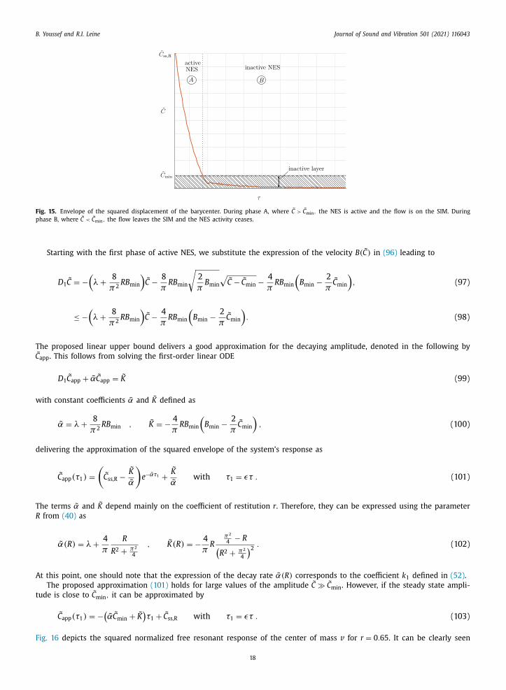
Fig. 15. Envelope of the squared displacement of the barycenter. During phase A, where ˜ C >

˜ C min , the NES is active and the flow is on the SIM. During

phase B, where ˜ C <

˜ C min , the flow leaves the SIM and the NES activity ceases.

C

Starting with the first phase of active NES, we substitute the expression of the velocity B ( ̃ C ) in (96) leading to

D 1 ̃ C = −

(λ +

8

π2 RB min

)˜ C − 8

πRB min

√

2

πB min

√

˜ C − ˜ C min −4

πRB min

(B min −

2

π˜ C min

), (97)

≤ −(λ +

8

π2 RB min

)˜ C − 4

πRB min

(B min −

2

π˜ C min

). (98)

The proposed linear upper bound delivers a good approximation for the decaying amplitude, denoted in the following by ˜ app . This follows from solving the first-order linear ODE

D 1 ̃ C app + ˜ α ˜ C app =

˜ K (99)

with constant coefficients ˜ α and

˜ K defined as

˜ α = λ +

8

π2 RB min , ˜ K = − 4

πRB min

(B min −

2

π˜ C min

), (100)

delivering the approximation of the squared envelope of the system’s response as

˜ C app (τ1 ) =

(˜ C ss,R −

˜ K

˜ α

)e − ˜ ατ1 +

˜ K

˜ αwith τ1 = ετ . (101)

The terms ˜ α and

˜ K depend mainly on the coefficient of restitution r. Therefore, they can be expressed using the parameter

R from (40) as

˜ α(R ) = λ +

4

π

R

R

2 +

π2

4

, ˜ K (R ) = − 4

πR

π2

4 − R (

R

2 +

π2

4

)2 . (102)

At this point, one should note that the expression of the decay rate ˜ α(R ) corresponds to the coefficient k 1 defined in (52) .

The proposed approximation (101) holds for large values of the amplitude ˜ C � ˜ C min . However, if the steady state ampli-

tude is close to ˜ C min , it can be approximated by

˜ C app (τ1 ) = −(

˜ α ˜ C min +

˜ K

)τ1 +

˜ C ss,R with τ1 = ετ . (103)

Fig. 16 depicts the squared normalized free resonant response of the center of mass v for r = 0 . 65 . It can be clearly seen

18


Fig. 16. Comparison of the analytically approximated envelope ˜ C app , the numerically approximated envelope ˜ C num from (97) and the numerically estimated

amplitude ˜ C of the squared displacement of the barycenter v during free decay for r = 0 . 65 ( R = 0 . 21 ).

that the closed form approximation from (101) delivers a good estimation of the numerical results. However, this holds only

if ˜ C >

˜ C min , i.e. as long as the NES is active. At this stage, the design goal revolves around optimizing the decaying behavior.

In other words, it aims to maximize the decay rate of the response, denoted by ˜ α(R ) , and minimize the upper bound of the

inactive layer, denoted by ˜ C min (R ) , for which the NES becomes inactive. Starting by differentiating (102) with respect to R

delivers

∂ ̃ α

∂R

=

4

π

π2

4 − R

2 (R

2 +

π2

4

)2 . (104)

Taking into account that 0 ≤ r ≤ 1 , one can infer that ∂ ̃ α∂R

> 0 for 0 ≤ R ≤ 1 . Hence, the strictly increasing function ˜ α(R )

attains its maximum value for R opt = 1 . Next, the expression of ˜ C min given by (48) is considered

˜ C min =

R

2

R

2 +

π2

4

⇒

∂ ̃ C min

∂R

=

π2

2

R (R

2 +

π2

4

)2 ≥ 0 for 0 ≤ R ≤ 1 . (105)

Eq. (105) shows that the inactivity level of the NES can be set to zero, if the coefficient of restitution r = 1 and therefore

R opt = 0 . We conclude that we have to a make a tradeoff between a high decay rate and a small bound of the inactive

layer. The smaller the coefficient of restitution r is, the larger is the coefficient R, leading to a faster decay of the amplitude

from

˜ C ss,R to ˜ C min . However, the minimal value of the amplitude that can be achieved using the VI NES, described by ˜ C min ,

increases with an increasing value of the coefficient R . A possible way to cope with this drawback, is to include more

parameters in the design of the NES such as the cavity length b. The influence of the parameter b on the decay rate has

to be investigated as well. Therefore, the absolute displacement of the primary mass M, denoted by q 1 ( t ) , is considered.

Substituting (5) and (6) into (4) yields for a small value of ε

q 1 ( t ) ≈ b √

˜ C ( εω 0 t ) sin ( ω 0 t + γ ) . (106)

Based on the previous results, the absolute displacement of the primary mass can be approximated according to

q 1 , app (t) = b

√

˜ C app ( εω 0 t ) sin ( ω 0 t + γ ) . (107)

In the following, the influence of the parameter b on the decay rate of the response is investigated for two different am-

plitude ranges, for which the approximation of the squared amplitude ˜ C app is expressed accordingly and where the time

instant t = 0 corresponds to the moment at which the external excitation is turned off. Without loss of generality, the initial

value of the absolute displacement q 10 can be expressed as

q 10 := q 1 , ss,R = b

√

˜ C ss,R sin γ . (108)

If the steady state amplitude ˜ C ss,R is close to ˜ C min , one can approximate the absolute displacement of the primary mass

using (103) by

q 1 , app (t) =

√

−b 2 (

˜ α ˜ C min +

˜ K

)εω 0 t +

(q 10

sin γ

)2

sin ( ω 0 t + γ ) , (109)

19


For this amplitude range, the decay of q 1 , app (t) is strongly dependent on the parameter b. On the one hand, large values of

b lead to a faster decay but enlarge the inactivity range of the NES. On the other hand, choosing small values of b might

result in a non-decaying response

lim

b→ 0 q 1 , app (t) =

q 1 , ss,R

sin ( γ ) sin ( ω 0 t + γ ) . (110)

For a larger amplitude range, i.e. ˜ C min � ˜ C ss,R <

˜ C max , the absolute displacement can be approximated through

q 1 , app (t) =

√ √ √ √

( (q 10

sin γ

)2

+

˜ K b 2

˜ α

)

e − ˜ αεω 0 t +

˜ K b 2

˜ αsin ( ω 0 t + γ ) , (111)

In this case, the decay of q 1 , app (t) is not much influenced by the value of b. In fact, the decay of the response is still mainly

dependent on R even for small values of b

lim

b→ 0 q 1 , app (t) =

q 10

sin ( γ ) sin ( ω 0 t + γ ) e −

1 2 ̃ αεω 0 t . (112)

Hence, the steady state amplitude at resonance ˜ C ss,R must be kept within the optimal range, i.e. ˜ C min � ˜ C ss,R <

˜ C max , by

tuning through both parameters b and R simultaneously. Moreover, from (112) , a further tuning parameter can be added by

considering the dimensionless damping, denoted in the following by D LO-NES , given by

D LO-NES =

1

2

ε ˜ α =

1

2

ελ +

1

2

ε4

π

R

R

2 +

π2

4

. (113)

The first term of (113) represents the damping ratio D LO of the linear oscillator from Fig. 1 without the embedded NES. In

fact, for a damped harmonic oscillator with mass M, damping coefficient c and spring constant k the damping ratio

D LO =

c

2

√

kM

, (114)

can be rewritten using (3) as

D LO =

1

2

m

M

c

m

√

M

k =

1

2

ελ . (115)

The second term of (113) represents the damping caused by the NES activity during the considered type of motion, denoted

by D NES . These results are in agreement with the previous findings and extend them to include the mass ratio ε as a

new tuning parameter. The damping effect of the NES does not only depend on the coefficient of restitution r but also

on the secondary mass m . Hence, for a small enough mass m, the larger R is, the greater the damping is and the faster

the amplitude decays over time. Another important aspect that should not be overlooked, concerns the activation threshold

of the NES. In other words, the stability borders of the SIM must be defined to guarantee a sustained activity of the NES

until the vanishing of the response. For an optimal design, the distance between the starting point on the SIM

˜ C ss,R and

its lowest point ˜ C min should be maximized, while minimizing the activation threshold. To this aim, we introduce the new

tuning variable ξ , being a dimensionless measure describing the width of the stability range and defined as

ξ ( R ) =

√

˜ C max ( R )

˜ C min ( R ) =

√ (R

2 +

π2

4

)(R

2 π2 + 4

)R

(π2

2 − 2

) for 0 ≤ R < 1 . (116)

The obtained expression is a decreasing function of R, which attains its minimum ξmin =

π2 +4 π2 −4

for R = 1 . For R = 0 , i.e. when

the activation threshold of the NES is set to zero, the function value tends towards infinity, lim R → 0 ξ ( R ) = ∞ . The function

ξ will be further used as a criterium to set up the design rules of the NES.

In a next step, a verification of these findings is carried out numerically. Specifically, the dependency of the normalized

barycentric response and the LO displacement on the parameter R and b is investigated through numerical simulations for

a fixed external excitation amplitude E. The squared resonant decaying response v 2 (given by ˜ C ) and the decaying resonant

response of the primary mass q 1 for different values of R and a fixed value of b are shown in Figs. 17 and 18 , respectively.

It is observed that both displacements v and q 1 decrease faster with the increase of R, due to the increase of the decay

rate ˜ α. Moreover, the distance between the starting point on the SIM

˜ C ss,R and its lowest point ˜ C min decreases due to the

decrease of ξ . Therefore, the attained steady state amplitude for the same excitation amplitude E decreases with the increase

of R, which accordingly yields a larger inactivity layer of the NES. This unwanted effect of a large R can be counteracted by

a smaller value of b. The variation of the parameter b while fixing the parameter R is depicted in Figs. 19 and 20 . It can be

clearly seen, that the cavity length has no effect on the activation threshold

˜ C min . However, even though the influence of

the parameter b on the normalized response cannot be directly recognized, the steady state amplitude ˜ C ss,R decreases with

the increase of b, which is due to a lower normalized excitation level G and can be deduced from (3) . Thereby, it can be

20


Fig. 17. Comparison of numerically estimated amplitude ˜ C of the free resonant response for different values of R and b = 0 . 015 . The dot-dashed lines

represent the corresponding values of the inactive layer ˜ C min .

Fig. 18. Comparison of numerically estimated envelope of the free resonant response of the primary mass q 1 for different values of R and b = 0 . 015 . The

dot-dashed lines represent the corresponding values of the inactive layer q 1 , min .

Fig. 19. Comparison of numerically estimated amplitude ˜ C of the free resonant response for different values of b and R = 0 . 21 . The dot-dashed lines

represent the corresponding values of the inactive layer ˜ C min .

21


Fig. 20. Comparison of numerically estimated envelope of the free resonant response of the primary mass q 1 for different values of b and R = 0 . 21 . The

dot-dashed lines represent the corresponding values of the inactive layer q 1 , min .

used for further tuning of the LO response, such as minimizing the steady state vibration amplitude or the NES activation

threshold (see Fig. 20 ) and therefore, enlarging the operating range.

According to this analysis, a complete vanishing of the response can be achieved for the parameter value b opt = 0 . As to

the optimal value of R, it results from a tradeoff between a small operating range and a high decay rate. Yet, these values

do not match a realistic and reasonable design. The first limitation concerns the coefficient of restitution r: the value r = 0 ,

for which the decay rate is at its maximum, represents an inelastic collision, after which the small mass remains in contact

with the wall and the considered type of motion with alternating collisions on the opposite wall of the cavity can not

occur. Therefrom, the use of the sawtooth function (21) is invalid and the conducted analysis fails. A second limitation with

regard to the cavity length arises as well, since the optimal value corresponds to a nonexisting cavity and therefore does not

correspond to the studied model. Based on these results und taking into account the discussed limitations, the design rules

for the studied VI NES can be set up as follows: Given a system model described by (1) and (2) , together with a desired

operating range, with the borders q d 1 , max

and q d 1 , min

, and a desired dimensionless damping D

d LO-NES

within the given range,

the design parameters of the NES can be chosen according to the following steps:

Step 1: The choice of the coefficient of restitution r Through the given desired amplitude range, the optimal value of R can

be chosen based on (116) . This criterion is to be met by choosing the desired maximal and minimal amplitudes q d 1 , max

and

q d 1 , min

such that they do not exceed the stability borders, i.e.

q d 1 , max < q 1 , max = b √

˜ C max ( R ) , q d 1 , min ≥ q 1 , min = b √

˜ C min ( R ) . (117)

The optimal value R opt satisfies

q d 1 , max

q d 1 , min

= ξ (R opt ) > ξmin with 0 ≤ R opt < 1 . (118)

and the corresponding value for the coefficient of restitution r opt is obtained using (40) , as

r opt =

1 − R opt

1 + R opt . (119)

If the ratio q d

1 , max

q d 1 , min

≤ ξmin , we choose R opt → 1 (and accordingly r opt → 0 ).

Step 2: The choice of the cavity length b For the chosen value R opt , the activation threshold of the NES ˜ C min (R opt ) as well

as the upper stability border ˜ C max (R opt ) are fixed. Therefore the cavity length is determined according to (117) as

q d 1 , max √

˜ C max (R opt ) < b ≤

q d 1 , min √

˜ C min (R opt ) , (120)

In fact, for small values of b, the upper bound of the inactive layer characterizing the NES can be further minimized even

for large values of ˜ C min .

Step 3: The choice of the auxiliary mass m As a last step, the NES damping ratio D NES is determined from the desired

dimensionless damping D

d LO-NES

within the given operating range using (113) and (114) as

D NES = D

d LO-NES −

c

2

√

kM

, (121)

22


Solving (113) using (115) for the obtained value of D NES and the chosen value for R opt yields

ε = D NES

π

2

R

2 opt +

π2

4

R opt , (122)

which can be reformulated to express the value of the auxiliary mass m as

m = M

(D

d LO-NES −

c

2

√

kM

)π

2

R

2 opt +

π2

4

R opt . (123)

Lastly, one should keep in mind that the mass ratio ε should be kept small enough to guarantee the validity of the assump-

tions behind the analytical results and therefore the desired NES damping must be chosen accordingly.

7. Conclusion

This paper shows how the multiple scales analysis can be used to extract a closed-form approximation of the backbone

curve of a nonlinear mode for a nonsmooth system. The analysis conducted in this paper answers the question: How can

the analytical results be used in a way that allows an optimal design of the impact absorber to assure an efficient mitigation

of the resonant vibrations? Here, the analysis has been done for symmetric 2 IPP motion of the single DOF LO-VI NES. The

merits and outcome of the paper are:

• The effective operating range of the VI NES corresponds to a wide, yet limited range of external excitation levels. How-

ever, the studied periodic motion occurs in the middle range of the external forcing amplitude.

• The phase resonance condition and the extended periodic motion concept yield, in combination with a two-scales first-

order multiple scales approximation, the same expression for the backbone curve.

• The shift of the resonance frequency and the damping effect of the VI NES are confirmed through numerical simulations.

• Two practical performance measures for the VI NES under harmonic forcing are proposed: the dimensionless tuning

variable ξ describing the absorber operating range and the dimensionless damping ratio D NES , quantifying the damping

caused by the NES activity.

• These performance measures are used to demonstrate that the energy pumping occurs only under nonconservative con-

tact conditions.

• The choice of the VI NES design parameters, i.e. cavity length, coefficient of restitution and auxiliary mass, for which the

vibration absorber is optimally active, depends on various requirements. Here, the range of the parameters in which low

amplitude periodic motion occurs is considered. The developed design strategy delivers a set of parameters for which

the occurrence of the symmetric 2 IPP motion is desirable and which is mainly based on the amplitude of the system’s

response, the desired damping ratio and the activation threshold of the VI NES.

Further research is needed to find out at which level of approximation the applied concepts differ in their approximation

of the backbone curve. Here, the analysis has been done for symmetric 2 IPP motion of the single DOF LO-VI NES, but the

same approach can be used for other normal modes of this system or for other systems, e.g. a hybrid VI NES [1] . It remains

to be investigated how this analysis can be generalized to a multi-DOF LO-VI NES system or to a single DOF LO multi-VI

NES [12,17] . At the end of the paper, the design rules for the VI NES are discussed and the chosen approach shows its merit:

the closed-form approximate solutions for the slow dynamics allows for a closed-form design strategy in which a trade-off

between decay rate and operating range has to be made. The presented results of direct numerical simulations agree with

the theoretical findings. They enclose a wide sufficient range of system parameters, which favors the practical realization

and experimental tuning of the NES. Further exploitation of these results will concern their extension and application to

more complex structures with possible mode interaction or the investigation of different response regimes around the SIM,

which may provide a deeper understanding of the VI NES dynamics.

Declaration of Competing Interest

The authors declare that they have no known competing financial interests or personal relationships that could have

appeared to influence the work reported in this paper.

CRediT authorship contribution statement

Balkis Youssef: Methodology, Formal analysis, Software, Investigation, Writing - original draft. Remco I. Leine: Concep-

tualization, Methodology, Writing - review & editing, Supervision, Funding acquisition.

23


Acknowledgement

This research was supported by the Deutsche Forschungsgemeinschaft , DFG, project number 402813361 .

Appendix A

Table 1

Parameters of the numerical LO-VI NES model.

Physical Parameters Normalized Parameters

M 3 . 807 kg ε 0 . 0084

c 2 . 53 Ns / m λ 1 . 4274

k 11 . 68 · 10 3 N / m R 0 . 2121

m 0 . 032 kg

b 0 . 015 m

r 0 . 65

Table 2

Parameters of the simu-

lated experiment.

PLL Tuning Parameter

�L 2

�VCO 0.9901

K p 0 . 0 0 0 0 01

K I 0 . 0 0 0 0 01

References

[1] M. Farid , O. Gendelman , V. Babitsky , Dynamics of a hybrid vibro-impact nonlinear energy sink, ZAMM (2019) e201800341 . [2] O. Gendelman , Analytic treatment of a system with a vibro-impact nonlinear energy sink, J. Sound Vibr. 331 (21) (2012) 4599–4608 .

[3] O. Gendelman , A. Alloni , Dynamics of forced system with vibro-impact energy sink, J. Sound Vibr. 358 (2015) 301–314 . [4] O. Gendelman , A. Alloni , Forced system with vibro-impact energy sink: chaotic strongly modulated responses, Procedia IUTAM 19 (1) (2016) 53–64 .

[5] O. Gendelman , Y. Starosvetsky , M. Feldman , Attractors of harmonically forced linear oscillator with attached nonlinear energy sink i: description of

response regimes, Nonlinear Dyn. 51 (1–2) (2008) 31–46 . [6] E. Gourc , G. Michon , S. Seguy , A. Berlioz , Experimental investigation and design optimization of targeted energy transfer under periodic forcing, J. Vibr.

Acoust. 136 (2) (2014) . [7] E. Gourc , G. Michon , S. Seguy , A. Berlioz , Targeted energy transfer under harmonic forcing with a vibro-impact nonlinear energy sink: analytical and

experimental developments, J. Vibr. Acoust. 137 (3) (2015) . [8] G. Kerschen , M. Peeters , J.-C. Golinval , A.F. Vakakis , Nonlinear normal modes, Part I: a useful framework for the structural dynamicist, Mech. Syst.

Signal Process. 23 (1) (2009) 170–194 .

[9] M. Krack , Nonlinear modal analysis of nonconservative systems: extension of the periodic motion concept, Comput. Struct. 154 (2015) 59–71 . [10] Y. Lee , A.F. Vakakis , L. Bergman , D. McFarland , G. Kerschen , F. Nucera , S. Tsakirtzis , P. Panagopoulos , Passive non-linear targeted energy transfer and its

applications to vibration absorption: a review, Proc. Inst. Mech.Eng. Part K 222 (2) (2008) 77–134 . [11] T. Li , Study of nonlinear targeted energy transfer by vibro-impact, Toulouse, INSA, 2016 Ph.D. thesis .

[12] T. Li , E. Gourc , S. Seguy , A. Berlioz , Dynamics of two vibro-impact nonlinear energy sinks in parallel under periodic and transient excitations, Int. J.Non-Linear Mech. 90 (2017) 100–110 .

[13] T. Li , S. Seguy , A. Berlioz , Dynamics of cubic and vibro-impact nonlinear energy sink: analytical, numerical, and experimental analysis, J. Vibr. Acoust.

138 (3) (2016) . [14] T. Li , S. Seguy , A. Berlioz , On the dynamics around targeted energy transfer for vibro-impact nonlinear energy sink, Nonlinear Dyn. 87 (3) (2017)

1453–1466 . [15] T. Li , S. Seguy , A. Berlioz , Optimization mechanism of targeted energy transfer with vibro-impact energy sink under periodic and transient excitation,

Nonlinear Dyn. 87 (4) (2017) 2415–2433 . [16] T. Li , S. Seguy , A. Berlioz , E. Gourc , Analysis of a vibro-impact nonlinear energy sink: theoretical and numerical developments, Congrès Français de

Mécanique, AFM, Association Française de Mécanique, 2015 .

[17] W. Li , N.E. Wierschem , X. Li , T. Yang , M.J. Brennan , Numerical study of a symmetric single-sided vibro-impact nonlinear energy sink for rapid responsereduction of a cantilever beam, Nonlinear Dyn. (2020) 1–21 .

[18] J.M. Londoño , S.A. Neild , J.E. Cooper , Identification of backbone curves of nonlinear systems from resonance decay responses, J. Sound Vibr. 348 (2015)224–238 .

[19] A.H. Nayfeh , Introduction to Perturbation Techniques, John Wiley & Sons, 2011 . [20] F. Nucera , A.F. Vakakis , D. McFarland , L. Bergman , G. Kerschen , Targeted energy transfers in vibro-impact oscillators for seismic mitigation, Nonlinear

Dyn. 50 (3) (2007) 651–677 .

[21] G. Pennisi , C. Stéphan , E. Gourc , G. Michon , Experimental investigation and analytical description of a vibro-impact NES coupled to a single-de-gree-of-freedom linear oscillator harmonically forced, Nonlinear Dyn. 88 (3) (2017) 1769–1784 .

[22] G. Pennisi , C. Stéphan , G. Michon , Vibro-impact NES: a correlation between experimental investigation and analytical description, in: Sensors andInstrumentation, Volume 5, Springer, 2016, pp. 137–142 .

[23] S. Peter , R. Riethmüller , R.I. Leine , Tracking of backbone curves of nonlinear systems using phase-locked-loops, in: Nonlinear Dynamics, Volume 1,Springer, 2016, pp. 107–120 .

24

https://doi.org/10.13039/501100001659

http://refhub.elsevier.com/S0022-460X(21)00115-2/sbref0001


































































































[24] D. Qiu , S. Seguy , M. Paredes , Design criteria for optimally tuned vibro-impact nonlinear energy sink, J. Sound Vibr. 442 (2019) 497–513 . [25] L. Renson , A. Gonzalez-Buelga , D. Barton , S. Neild , Robust identification of backbone curves using control-based continuation, J. Sound Vibr. 367 (2016)

145–158 . [26] M. Sayed , M. Kamel , Stability study and control of helicopter blade flapping vibrations, Appl. Math. Modell. 35 (6) (2011) 2820–2837 .

[27] J. Shaw , S.W. Shaw , A.G. Haddow , On the response of the non-linear vibration absorber, Int. J. Non-Linear Mech. 24 (4) (1989) 281–293 . [28] A.F. Vakakis , O.V. Gendelman , L.A. Bergman , D.M. McFarland , G. Kerschen , Y.S. Lee , Nonlinear Targeted Energy Transfer in Mechanical and Structural

Systems, vol. 156, Springer Science & Business Media, 2008 .

25
























journal of sound and vibration - uni-stuttgart.de

Documents