Journal of Researchn ~~ .f>4nC f 4 4Th ede a>x

?v'2S';1,- ~~~ *

volume 90 Number 6 November-December

Special Issue: Chemometrics Conference Proceedings

Topical Issue: ChemometricsHans J. Oser, Chief Editor .

Jack YoudenHHM. Ku and JR. DeVoe .

The Organizers' GoalsClifford H Spiegelman, Robert L. Watters, Jr., and Jerome Sacks.

Agenda for ChemometriciansWilliam G. Hunter.

Adaptive Kalman FilteringSteven D. Brown and Sarah C Rutan .

The Limitations of Models and Measurements as RevealedThrough Chemometric IntercomparisonL.A. Currie.

DISCUSSION - Leon Jay Geser .

Statistical Properties of a Procedure for Analyzing PulseVoltammetric DataThomas P. Lane, John J. O'Dea, and Janet Osteryoung .

DISCUSSION - Janet Os-erytung.

Fitting First Order Kinetic Models Quickly and EasilyDouglas M. Bates and Donald G. Watts .

DISCUSSION - Michael Frenklach .

The Use of Kalman Filtering and Correlation Techniquesin Analytical Calibration ProceduresH C. Smit .

DiSCUSSION - Diane Lambert.

Intelligent InstrumentationAlice M Harper and Shirley A. Liebman .

DISCUSSION - Richard J Beckman.

The Regression Analysis of Collinear DataJohn Mandel ....... -.

DISCUSSION -R. W Gerlach ..........................

OptimizationStanley N Deming .....................

DISCUSSION - C.K. Bayne ..........

391

393

395

397

403

409

419

423

430

433

438

441

451

453

464

465

477

479

483

Strategies for the Reduction and Interpretation of MulticomponentSpectral DataIsiah M Warner, S.L. Neal, and TM Rossi...................................

Some New Ideas in the Analysis of Screening DesignsGeorge Box and R. Daniel Meyer ...........................................

DISCUSSION - Vijayan Nair and Michael Frenklach ........................

Polymers and Random Walks - Renormalization Group Descriptionand Comparison with ExperimentKarl F. Freed ........................................................Fourier Representations of Pdfs Arising in CrystallographyGeorge H. Weiss and Uri Shmuef.

DISCUSSION - £E Prince .

Aggregated Markov Processes and Channel Gating KineticsDonald R. Fredkin and John A. Rice .....................................

Automated Pattern Recognition: Self-Generating Expert Systemsfor the FutureThomas L. Isenhour...................................................

Regression Analysis of Compartmental ModelsT.L. Lai..............................................................

DISCUSSION - T.-H. Peng..............................................

Measurement and Control of Information Content in ElectrochemicalExperimentsSam P. Perone and Cheryl L. Ham ..........................................

DISCUSSION - Herman Chernoff............................

Pattern Recognition Studies of Complex Chromatographic Data SetsP.C hurs, BK. Lavine, and TR. Stouch ....... ............................... 543

ISSN 0160-1741 Library of Congress Catalog Card No.: 63-37059

The Journal of Research of the National Bureau of Standards features advances in measurementmethodology and analyses consistent with the NBS responsibility as the nation's measurement sciencelaboratory. It includes reports on instrumentation for making accurate and precise measurements infields of physical science and engineering, as well as the mathematical models of phenomena whichenable the predictive determination of information in regions where measurements may be absent.Papers on critical data, calibration techniques, quality assurance programs, and well characterizedreference materials reflect NBS programs in these areas. Special issues of the Journal are devoted toinvited papers in a particular field of measurement science. Occasional survey articles and conferencereports appear on topics related to the Bureau's technical and scientific programs.

Hans J. Oser. Chief EditorExecutive Editors Board of EditorsDonald R. Johnson John W. Cooper (Physics) Howard J. M. Hanley(Natl. Measurement Lab.) Sharon G. Lias (Chemistry) (Boulder Laboratory)John W. Lyons Donald G. Eitzen (Engineering) John W. Cahn (Materials)(Nati. Engineering Lab.)

Issued six times a year. Annual subscriptions: domestic $17.00; foreign $21.25. Single copy, $3.00domestic; $3.75 foreign.

United States Government Printing Office, Washington: 1985Order all publications from the Superintendent of DocumentsU.S. Government Printing Office, Washington, DC 20402

The Secretarytransaction ofperiodical has1, 1986.

of Commerce has determined that the publication of the periodical is necessary in thethe public business required by law of this Department. Use of funds for printing thisbeen approved by the Director of the Office of Management and Budget through April

487

495

501

*.. 503

.... 507

.. 513

517

521

525

530

531

.......... .. ....539

chemometricsconference

Topical Issue: Chemometrics

This issue of the NBS Journal of Research is devoted entirely to one topic:Chemometrics. A conference by that title held earlier this year at NBS brought togetherexperts in analytical chemistry and applied mathematics, disciplines which are theconstituents of this new field. This conference was probably the first one in the UnitedStates by that title.

The roots of the interdisciplinary effort go back to the late Dr. William (Jack) Youdenand we dedicate this issue to him. A brief description of Youden's career serves as theintroduction to the collection of conference papers which we present in this volume ofthe JournaL The authors of this biographical sketch, Drs. Ku and DeVoe, worked veryclosely with Youden while he was at NBS.

With the publication of the papers presented at this conference we hope to stimulatefurther work in the field of chemometrics. Special recognition goes to the organizers ofthe conference who also served as invited editors of this special issue of the NBSJournal of Research: Drs. Clifford H. Spiegelman of the Center for AppliedMathematics, Robert L. Watters of the Center for Analytical Chemistry, and JeromeSacks from the University of Illinois.

Hans J. OserChief Editor

391

JACK YOUDEN

We are pleased that the Conference proceedings are dedicated to Jack Youden.

Youden, an analytical chemist turned mathematical statistician, was a simplifyingand, indeed, enthralling teacher of statistical principles who could hold the attentionof sophisticated statisticians as well as scientists and engineers.

Born at the turn of the century, Youden worked for many years at the BoyceThompson Institute for Plant Research in Yonkers, NY before joining the staff atNBS in 1948. He remained with the Bureau for 17 years and after his retirementcontinued this association as a guest worker until his death in 1971.

The transformation of Youden from chemist to statistician probably began with hisreading of R. A. Fisher's Statistical Methods for Research Workers. He studied underFisher in 1937-38 at the Galton Laboratory of University College, London, thanksto a Rockefeller Fellowship for the discovery of a new class of incomplete blockdesigns, "Youden Squares," which found immediate application in biological andmedical research.

At NBS he introduced "Youden Plots" for interlaboratory tests and "Youden'sRuggedness Test" as a check on test methods, but he distinguished himself prin-cipally for his ability to reduce a complicated idea to its essentials and to express thatidea in a simple, straightforward manner, so that it became understandable to sci-entists of all disciplines. He worked hard at stripping away needless detail andjargon. And he generated interest in his lectures, making his subject so intriguingthat an hour passed as minutes. He was a very rare breed-an outstanding statisticianwho understood experimental systems in chemistry, physics, and engineering.

His first book, Statistical Methods for Chemists, was published in 1951 and wasfollowed by Statistical Techniques for Collaborative Tests which consisted of two

393

Youden lecture series, "Accuracy of Analytical Procedures" and "The Collabo-rative Test." The latter book was published by the Association of Official AnalyticalChemists (AOAC) whose William Horwitz states: "These lectures probably havehad a greater influence on improving the quality and interpretation of collaborativestudies conducted by AOAC members than any other event in the (85-year) exis-tence of the Association."

A number of Youden's most important papers were collected in the Journal ofQuality Technology (Vol. 4, No. 1, January 1972) and in Volume I of NBS SpecialPublication 300, Precision Measurement and Calibration: Statistical Concepts andProcedures.

Jack Youden was a chemist and a communicator. The Chemical Division of theAmerican Society for Quality Control in 1969 established a Jack Youden prize to beawarded yearly for the best expository paper in its journal, Technometrics. But it wasYouden the statistician who furthered collaboration and helped to maximize theinformation content of experimentation, which is what the Chemometrics Confer-ence was about. So it is appropriate that these conference proceedings be dedicatedto the memory of Dr. Youden.

H. H. Ku J. R. DeVoeStatistical Engineering Division Inorganic Analytical Research DivisionNational Bureau of Standards National Bureau of Standards

394

The Organizers' Goals

The wide range of disciplines represented by the participants and attendees of the Chemomet-rics Research Conference held at the Gaithersburg Holiday Inn on May 20-22, 1985, exempli-fies the depth and diversity of the chemometrics community. The Conference was sponsored byseveral important professional societies whose members are involved in chemometric activity.These include the Analytical Division of the American Chemical Society, the Section onPhysical and Engineering Sciences of the American Statistical Association, the Institute ofMathematical Statistics, and the Society for Applied Spectroscopy. Generous funding for theConference was provided by the National Bureau of Standards, the Office of Naval Research,and the National Science Foundation.

As organizers, we had two main goals in mind when deciding on the form and substance ofthe Conference. The first was to provide a forum for reporting on some of the most recent andimportant research activities in diverse areas relating to chemometrics. Nineteen invited speak-ers covered topics including experimental design and optimization, kinetic rate constants,Kalman filtering, chromatography, data analysis, artificial intelligence, stochastic processes,regression and factor analysis. Despite the full schedule of papers, each of the five sessions wasattended by nearly all of the 134 Conference registrants. Most of the papers are published in thisspecial issue of the National Bureau of Standards Journal of Research to provide the registrantsand others the opportunity for careful study of the presentations. In these respects, our first goalwas easier to achieve than the second.

Our second and more important goal can only be achieved gradually. This was to increase thewillingness of chemists, statisticians, and probabilists to meet as colleagues and to solveproblems as a team. This will necessarily involve the exercise of communication skills as wellas the combining of scientific skills. We believe that even the best separate efforts of chemistsand mathematicians fall far short of the achievements that are possible by joint efforts inchemometric research teams. We underscored this aspect of teamwork between the disciplinesof chemistry and mathematics by having each invited paper in one discipline discussed by aninvited discussant of the other.

We invited the speakers to take any approach they desired in the exposition of their subject.Hence, the papers range from strictly technical to philosophical in tone. Discussants also had theoption of either commenting on the specifics of a given paper, or exploring the relevance of the

395

subject to their respective disciplines. This free format encouraged open discussion and ex-change of ideas at the Conference, and we hope that the same stimulus will be provided by theseProceedings.

Finally, we look forward to future chemometrics conferences organized by researchers withperspectives other than our own. For no matter how broad the coverage of chemometrics topicsin a given program, important areas are omitted. We believe that the widest scope of chemomet-ncs research activities can be presented in meetings organized by committees of differentbackgrounds and insights.

Clifford H. SpiegelmanNational Bureau of Standards

Robert L. Watters, Jr.National Bureau of Standards

Jerome SacksUniversity of Illinois, Urbana

396

Agenda for Chemometricians

It is most appropriate that the proceedings of this conference are going to be dedicated to thememory of Jack Youden. He was interested in many of the topics that are being considered at

this conference, for example, interlaboratory comparisons, calibration, analytical methods, andmeasurement errors-both systematic and random. He was indeed a pioneering chemometri-cian, before the name existed. He was also interested in explaining to chemists, chemicalengineers, and others how they could benefit by using statistical methods.

I'm sure Youden would have been pleased with this conference, which provides a forum forchemists, statisticians, and others interested in chemometrics to discuss research of mutualinterest. He also might have observed that chemometrics as a field has reached a level of

maturity that warrants consideration of questions related to spreading the word to others, tonon-chemometricians, so that they could take advantage of the techniques that are now avail-able. In other words, perhaps chemometrics as discipline has reached a sufficiently advanced

stage of research and development that questions of production should now be addressed. Whatare our most useful products? Who are out customers? Which products would they find mostvaluable? What are the obstacles that prevent these customers from using these products now?How can these obstacles be overcome? What are the most important things that can be done inthe next three years to reach new customers? What should the agenda be for chemometriciansin the next few years?

There are two ways to learn. One is to listen, as in a lecture. The other is to engage in adialogue, as in a conversation. The first way is passive. The second is active. Let's try thesecond way to learn from one another how we might answer these questions.

[Participants at this point wrote out answers to these questions, discussed them, and voted onthem. The top vote-getters for the most important things that can be done in the next three yearsto reach new customers were the following, listed in order of decreasing number votes:

1. Organize joint conferences with chemists.2. Write textbooks on chemometrics.3. Conduct workshops and teach short courses.4. Write user-friendly software.5. Teach chemometrics to graduate students.

397

6. Write tutorial, expository, and review articles.7. Undertake joint research projects with chemists.8. Publicize success stories.9. leach chemometrics to undergraduate students.

10. Communicate with management.11. Hire professionals to help with a public relations effort.12. Teach chemometrics to high school students.]I recommend that we take action on the basis of this list. Let me now make a few observations

in closing. I would like to suggest a different starting point for statistics courses. Let us representthe relationship between an observed response y and variables xl,.x2 ,. . . as

y=f(X1 ,x2 ,X3 ,X4.X5 . * x,126,. * ) -

Many, many, many variables affect y. It is the fluctuation of these variables that gives usdifferent answers when we repeat an experiment two or more times under "identical conditions."We are often interested in creating a mathematical equation (model) that involves a subset of thevariables. For purposes of illustration, suppose this subset is (x ,x9.A. We can then write

Note that the g function includes xl and x2 (because of lack of fit of the model) as well as allthe other x's. Lack of fit occurs, for example, because the model f may be taken to be linearinxl andx 2 but the actual relationship may be nonlinear in xi and x2. The function g is most oftencalled experimental error, and it is almost as often endowed by writers with an abundance ofdesirable and well-known properties. They call it a random variable. A sequence of theseexperimental errors, they frequently say, can be assumed to be independent, identically dis-

tributed according to a Normal distribution with a zero mean and constant variance. I believethat statisticians too readily make this assumption and others like it. Sometimes such an assump-tion makes sense, sometimes not. We should be more careful on this point.

An adequate model is a function that will turn data into white noise, as George Box has said.An analogy that I find useful involves a process for separating gold particles from a slurry. Ifthe process is fully efficient, the waste stream will contain no gold. It is therefore prudent tocheck the waste stream to see if it contains any gold. Likewise in creating and fitting models,it makes sense to examine residuals to see if they contain any information. The data containinformation (that's the gold we want to get), and a good model will extract all the informationin those data. Hence the residuals will be manifestations of white noise, an informationlesssequence of values.

Chemists and chemical engineers could benefit from knowing more about variance compo-nents, statistical graphics, and quality control techniques (including Shewhart and cumulativesum charts). But, above all, I think they would find statistical experimental designs to be themost useful thing of all that chemometricians have to offer. Such designs provide a practicalmeans for increasing research efficiency, which might be defined as the amount of informationone obtains per dollar spent.

The damage done by poor experimental design is irreparable. A poor design results in datathat contain little information. Consequently, no matter how thorough, how clever, or howsophisticated the subsequent analysis is, little information can be extracted. A good design, forthe same expenditure of time, money, and other resources, results in data rich in information.A fruitful analysis is then possible. (Note that analysis is defined as trying to extract all the usefulinformation in the data.)

Two-level factorial and fractional factorial designs can be extremely useful for chemists,chemical engineers, and others who do similar work. One of the best ways for a student to learnabout such designs is to set one up, get the data, analyze them, and interpret the results. For anumber of years I have had students in our experimental design course undertake such projects.

398

The main piece of advice I give them is to work on something they care about, something they

are really interested in.Toward the end of an introductory one-semester undergraduate course in statistics, for exam-

ple, one student said that he was a pilot and that, ever since he started to fly, he had asked

instructors and other pilots what he should do if the engine failed on takeoff. He had been told

by several people that he should bank the plane, go into a 1800 turn, and land on the runwayfrom which he took off. Unfortunately, many different ways of doing this maneuver had beensuggested. He successfully organized and executed a replicated 23 factorial design with three

variables: bank angle, flap angle, and speed. He measured the loss in altitude. He started each

test at 1000 feet instead of ground level. The experiment was a success. He learned which

combination of factors he should use for his plane, and he discovered the minimum altitude forattempting such a maneuver.

Factorial designs can be understood and run with profit by graduate, undergraduate, seniorhigh school, and junior high school students. Maybe younger students can use them, too.

Students can study the baking of cakes, the riding of bicycles, the making of chemicals, thegrowing of plants, and the swinging of pendulums. Dalia Sredni, when she was a seventh grader,

for instance, studied the effects of changing oven temperature, baking time, and the amount of

baking soda when making a cake. Students should be told about factorial designs early so thatthey can study systems that depend on many variables and learn how they work. Using suchdesigns they can discover interesting things, have fun, and be surprised. Our students deservemore of these pleasures. I have included a list of 101 experiments that have been done bystudents at Wisconsin, to indicate the variety of things that is possible.

I would like to end by congratulating the conference organizers for the excellent job they havedone. It is clear that they have worked hard to make-things enjoyable and rewarding for thoseof us who have been fortunate enough to participate.

William G. Hunter

Professor of Statistics and Industrial EngineeringDirector of Center for Quality and Productivity ImprovementUniversity of Wisconsin-Madison

Table 1. List of some studies done by students in an experimental design course at the University of Wisconsin-Madison.

variables responses

I. seat height (26, 30 inches), generator (off, on), tire pressure (40, 55 psi) time to complete fixed course on bicycle and pulserate at finish

2. brand of popcorn (ordinary, gourmet), size of batch (1/3, 2/3 cup), popcorn to oil yield of popcornratio (low, high)

3. amount of yeast, amount of sugar, liquid (milk, water), rise temperature, rise time quality of bread, especially the total rise

4. number of pills, amount of cough syrup, use of vaporizer how well twins, who had colds, slept during the night

5. speed of film, light (normal, diffused), shutter speed quality of slides made close up with flash attachmenton camera

6. hours of illumination, water temperature, specific gravity of water growth rate of algae in salt water aquarium

7. temperature, amount of sugar, food prior to drink (water, salted popcon) taste of Koolaid

8. direction in which radio is facing, antenna angle, antenna slant strength of radio singal from particular AM station inChicago

9. blending speed, amount of water, temperature of water, soaking time before blend- blending time for soy beans

big

399

Tahie 1. continued

variables responses

10. charge time, digits fixed, number of calculations perfonmed operation time for pocket calculator

11. clothes dryer (A. B), temperature setting, load time until dryer stops

12. pan (aluminum, iron), burner on store, cover for pan (no, yes) time to boil water

13. aspirin buffered? (no. yes), dose, water temperature hours of relief from migraine headache

14. amount of milk powder added to milk, heating temperature, incubation temperature taste comparison of homemade yogurt and commercialbrand

15. pack on back (no. yes), footwear (tenmis shoes, boots), run (7, 14 flights of steps) time required to run up steps and heartbeat at top

16. width to height ratio of sheet of balsa wood, slant angle, dihedral angle, weight length of flight of model arplaneadded, thickness of wood

17. level of coffee in cup, devices (nothing, spoon placed across top of cup facing up), how much coffee spilled while walkingspeed of walking

18. type of stitch, yarn guage, needle size cost of knitting scarf, dollars per square toot

19. type of drink (beer, mm), number of drinks. rate of drinking, hours after last meal time to get steel ball through a maze

20. size of order, time of day, sex of server cost of order of french fries, in cents per ounce

21. brand of gasoline, driving speed, temperature gas mileage for car

22. stamp (first class, air mail), zip code (used, not used), time of day when letter number of days required for letter to be delivered tomailed another city

23. side of face (left, right), beard history (shaved once in two years-sideburns, shaved length of whiskers 3 days after shavingover 600 times in two years-just below sideburns)

24. eyes used (both, right), location of observer, distance number of times (out of 15) that correct gender ofpasserby was determined by experimenter with pooreyesight wearing no glasses

25. distance to target, guns (A, B), powders (C, D) number of shot that penetrated a one foot diametercircle on the target

26. oven temperature, length of heating, amount of water height of cake

27. strength of developer, temperature, degree of agitation density of photographic film

28. brand of rubber hand, size, temperature length of rubber band before it broke

29. viscosity of oil, type of pick-up shoes, number of teeth in gear speed of H.C.. scale slot racers

30. type of tire, brand of gas, driver (A, B) time for car to cover one-quarter mile

31. temperature, stirring rate, amount of solvent time to dissolve table salt

32. amounts of cooking wine, oyster sauce, sesame oil taste of stewed chicken

33. type of surface, object (slide rule, ruder, silver dollar), pushed? (no, yes) angle necessary to make object slide

34. ambient temperature, choke setting, number of changes number of kicks necessary to start motorcycle

35. temperature, location in oven, biscuits covered while baking? (no, yes) time to bake biscuits

36. temperature of water, amount of grease, amount of water conditioner quantity of suds produced in kitchen blender

37. person putting daughter to bed (mother, father), bed time, place (home, grandpar- toys child chose to sleep withents)

38. amount of light im room, type of music played, volume correct answers on simple arithmetic test, time re-quired to complete test, words remembered (from listof t1)

39. amounts of added Turkish, Latakia, and Perique tobaccos bite, smoking characteristics, aroma, and taste of to-bacco mixture

40. temperature, humidity, rock salt time to melt ice

41. number of cards dealt at one time, position of picker relative to the dealer points in games of sheepshead, a card game

42. marijuana (no, yes), tequiDa (no, yes), sauna (no, yes) pleasure experienced in subsequent sexual intercourse

400

Table 1. continued

variables responses

43. amounts of flour, eggs, milk taste of pancakes, consensus of group of four livingtogether

44. brand of suntan lotion, altitude, skier time to get sunburned

45. amount of sleep the night before, substantial exercise during the day? (no, yes), eat soundness of sleep, average reading from 5 persons

right before going to bed? (no, yes)

46. brand of tape deck used for playing music, bass level, treble level, synthesizer? (no, clearness and quality of sound, and absence of noise

yes)

47. Type of filter paper, beverage to be filtered, volume of beverage time to filter

48. type of ski, temperature, type of wax time to go down ski slope

49. ambient temperature for dough when rising, amount of vegetable oil, number of four quality characteristics of pizzaonions

50. amount of fertilizer, location of seeds (3X3 Latin square) time for seeds to germinate

51. speed of kitchen blender, batch size of malt, blending time quality of ground malt for brewing beer

52. soft drink (A, B), container (cm, bottle), sugar free? (no, yes) taste of drink from paper cop

53. child's weight (13, 22 pounds), spring tension (4, 8 cranks), swing orientation number of swings and duration of these swings ob-

(level, tilted) tained from an automatic infant swing

54. orientation of football, kick (ordinary, soccer style), steps taken before kick, shoe distance football was kicked(soft, hard)

55. weight of bowling ball, spin, bowling lane (A, B) bowling pins knocked down

56. distance from basket, type of shot, location on floor number of shots made (out of 10) with basketball

57. temperature, position of glass when pouring soft drink, amount of sugar added amount of foam produced when pouring soft drinkinto glass

58. brand of epoxy glue, ratio of hardener to resin, thickness of application, smoothness strength of bond between two strips of aluminum

of surface, curing time

59. amount of plant hormone, water (direct from tap, stood out for 24 hours), window root lengths of cuttings from purple passion vine after

in which plant was put 21 days

60. amount of detergent (1/4, 1/2 cup), bleach (none, I cup), fabric softener (not used, ability to remove oil and grape juice stains

used)

61. skin thickness, water temperature, amount of salt time to cook chinese meat dumpling

62. appearance (with and without a crutch), location, time time to get a ride hitchhiking and number of cars thatpassed before getting a ride

63. frequency of watering plams, use of plant food (no, yes), temperature of water growth rate of house plants

64. plunger A up (slow, fast), plunger A down (slow, fast), plunger B up (slow, fast) reproducibility of automatic dilutor, optical density

plunger B down (slow, fast) readings made with spectrophotometer

65. temperature of gas chromatograph column, tube type (U, J), voltage size of unwanted droplet

66. temperature, gas pressure, welding speed strength of polypropylene weld, manual operation

67. concentration of lysozyme, pH, ionic strength, temperature rate of chemical reaction

68. anhydrous barium peroxide powder, sulfur, charcoal dust length of time fuse powder burned and the evennessof burning

69. air velocity, air temperature, rice bed depth time to dry wild rice

70. concentration of lactose crystal, crystal size, rate of agitation spreadability of caramel candy

71. positions of coating chamber, distribution plate, and lower chamber number of particles caught in a fluidized bed collector

72. proportional band, manual reset, regulator pressure sensitivity of a pneumatic valve control system for aheat exchanger

73. chloride concentration, phase ratio, total amine concentration, amount of preserva- degree of separation of zinc from copper accom-

five added plished by extraction

401

Table 1. continued

variables responses

74. temperature, nitrate concentration, amount of preservative added measured nitrate concentration in sewage, comparison

of three different methods

75. solar radiation collector size, ratio of storage capacity to collector size, extent of efficiency of solar space-heating system, a computershort-term intermittency of radiation, average daily radiation on three successive simulationdays

76. pH, dissolved oxygen content of water, temperature extent of corrosion of iron

77. amount of sulfuric acid, time of shaking milk-acid mixture, time of final tempering measurement of butterfat content of milk

78. mode (batch, time-sharing), job size. system utilization (low, high) time to complete job on computer

79. flow rate of carrier gas, polarity of stationary liquid phase, temperature two different measures of efficiency of operation ofgas chromatograph

80. pH of assay buffer, incubation time. concentration of binder measured cortisol level in human blood plasma

81. aluminum, boron. cooling time extent of rock candy fracture of cast steel

82. magnification, read out system (micrometer, electronic), stage light measurement of angle with photogrammetric instru-ment

83. riser height, mold hardness, carbon equivalent changes in height, width, and length dimensions ofcast metal

84. amperage, contact tube height, travel speed, edge preparation quality of weld made by submerged arc welding pro-cess

85. time, amount of magnesium oxide, amount of alloy recover of material by steam distillation

86. pH, depth, time final moisture content of alfalfa protein

87. deodorant, concentration of chemical, incubation time odor produced by material isolated from decaying ma-nure, after treatment

88. temperature variation, concentration of cupric sulfate concentration of sulfuric acid limiting currents on totaling disk electrode

89. air flow, diameter of bead, heat shield (no, yes) measured temperature of a heated plate

90. voltage, warm-up procedure, bulb age sensitivity of riicrodensitometer

91. pressure, amount of ferric chloride added, amount of lime added efficiency of vacuum filtration of sludge

92. longitudinal feed rate, transverse feed rate, depth of cut longitudinal and thrust forces for surface grinding op-eration

93. time between preparation of sample and refluxing, reflux time, time between end of chemical oxygen demand of samples with samereflux and start of titrating amount of waste (acetanilide)

94. speed of rotation, thrust load, method of lubrication torque of taper roller bearings

95. type of activated carbon, amount of carbon, pH adsorption characteristics of activated carbon usedwith municipal waste water

96. amounts of nickel, manganese, carbon impact strength of steel alloy

97. form (broth, gravy), added broth (no, yes), added fat (no, yes), type of meat (lamb, percentage of panelists correctly identifying whichbeet) samples were lamb

98. well (A, B), depth of probe, method of analysis (peak height, planimeter) methane concentration in completed sanitary landfill

99. paste (A, B), preparation of skin (no, yes), site (sternum, forearm) electrocardiogram reading

100. lime dosage, time of flocculation, mixing speed removal of turbidity and hardness from water

101. temperature difference between surface and bottom waters, thickness of surface mixing time for an initially thermally stratified tank oflayer, jet distance to thermocline, velocity of jet, temperature difference between jet waterand bottom waters

402

Journal of Research of the National Bureau of StandardsVolume 90, Number 6, November-December 1985

Adaptive Kalman Filtering

Steven D. Brown

Washington State University, Pullman, WA 99164

and

Sarah C. Rutan

Virginia Commonwealth University, Richmond, VA 23284

Accepted: June 24, 1985

The increased power of small computers makes the use of parameter estimation methods attractive. Suchmethods have a number of uses in analytical chemistry. When valid models are available, many methods workwell, but when models used in the estimation are in error, most methods fail. Methods based on the Kalmanfilter, a linear recursive estimator, may be modified to perform parameter estimation with erroneous models.Modifications to the filter involve allowing the filter to adapt the measurement model to theexperimental datathrough matching the theoretical and observed covoriance of the filter innovations sequence. The adaptivefiltering methods that result have a number of applications in analytical chemistry.

Key words: automated covariance estimation; Kalman filter; multicomponent analysis.

1. Introduction

The increased computational power available fromsmall computers has prompted a re-evaluation of themethods used in reducing data obtained from a chemicalanalysis. Many of the responses obtained from chemicalanalyses are suited to mathematical analysis by methodswhich estimate the parameters that generate the re-sponse; these parameters are generally concentrations.For parameter estimation to be successful, an accuratemodel of the behavior of the chemical system is neces-sary. The model used need not be theoretical; empiricalmodels based on experimental results or on a numericalsimulation of the chemical system are often satisfactory

About the Authors, Paper: Steven D. Brown is nowwith the Department of Chemistry at the Universityof Delaware. While Sarah C. Rutan, who was withWashington State University under a Summer Fel-lowship of the Analytical Division, American Chem-ical Society, is now with the Department of Chem-istry at Virginia Commonwealth. The workdescribed was supported by the Division of ChemicalSciences, U.S. Department of Energy.

as well. When valid models are available, the parametersassociated with the model may be obtained with a vari-ety of methods. Some that have seen extensive use inanalytical chemistry include analysis of the chemicaldata using linear least squares [1], nonlinear least squaresanalysis [2,3], and Kalman filtering [4-6].'

The methods mentioned above all work well withaccurate models, but are much less satisfactory whenused with models containing errors that can arise frommany sources. Theoretical models, or models based onsimulation, may not describe the physics or chemistry ofa system well enough to predict system responses to theaccuracy desired. Small changes in the experimentalconditions used for data acquisition may perturbexperimentally-obtained models, leading to errors whenthese models are used to analyze subsequent experi-ments. And, it may be impossible, because of the effectsof chemical equilibria, to obtain independent responsesfor some of the chemical species included in a model fora complex system, leading to "chemical" model errors.

Relatively few methods have been developed to com-pensate for model errors affecting multicomponentquantitation. Approaches using factor analysis [7] have

Bracketed figures indicate literature refrencrs.

403

been developed for situations where the model is un-known, but these approaches are generally limited tovery few components [8], and it is difficult to incorpo-rate additional a priori information into such methods.An alternative approach has used the Kalman filter. TheKalman filter is a linear, recursive estimator whichyields optimal estimates for parameters associated witha valid model [9,10]. Several methods, classified underthe term "adaptive filtering," have been developed topermit the filter to produce accurate parameter esti-mates in the presence of model errors [11-151. This pa-per summarizes the development of an adaptive Kalmanfilter for use in the mathematical analysis of overlappedmulticomponent chemical responses.

2. Theory

Kalman Filtering. The Kalman filter has receivedsome attention for the analysis of multicomponentchemical responses [4,6,16,17]. Because most models re-lating chemical responses to concentrations are linear,application of the Kalman filter is straightforward. Thefilter model is comprised of two equations. The systemmodel, which describes the time evolution of the desiredparameters, is, in state-space notation

X(k)=F(k,k - I)X(k - 1)+w(k) (2.1)

where X is a n X I column vector of state variables de-scribing the chemical system, where F is an n X n matrixdescribing how the states change with time, w is a vectordescribing noise contributions to the system model, andwhere k indicates time or some other independent vari-able which meets the noise requirements given below.For state-invariant systems, F reduces to the identitymatrix 1. Because multicomponent analysis is most oftenperformed under conditions where concentrations areconstant over the time frame involved, the case where Xis time-invariant is considered here.

The second equation describes the measurement pro-cess by relating the measured response z(k), to the filterstates. For a single sensor, the measurement model isgiven by

z(k) =HT(k)X(k)+v(k)

surement model is easily extended to systems with mul-tiple sensors.

The two noise processes in the Kalman filter, w(k)and v(k), are usually assumed to be independent, zero-mean, white noise processes. The matrix Q(k), definedas the covariance of the noise in the system model, istaken as approximately zero for the time invariant sys-tem discussed in this paper. The scalar quantity R(k) isthe variance of the noise in the measurement process.

The Potter-Schmidt square-root algorithm, one im-plementation of the Kalman filter [18], is given in table1. The details of this algorithm have been discussedelsewhere [18,19]. Initial guesses for the filter states andfor the covariance matrix P are required to start thefilter. Estimates of X and P depend on k, and becauseboth are projected ahead of the data (in eqs 2.3 and 2.4)by the filter, the notation (j I k) is used to indicate thatthe estimate is made at pointj, based on data obtained upthrough point k. The filter output consists of estimatesX, as well as P. In analytical chemistry, these are oftenestimates of concentrations and of the error in the con-centrations.

Table 1. Algorithm equations for the square root Kalman filter.

State estimate extrapolationX(k Ik - 1)=-F(k Ik - 1).X(k - IIk - I)

Covariance square root extrapolationS(k I k- 1)=F(k,k - 1)-(k - I| k -1).Fr(k,k - )

where

F(k,k - 1)=1

p=S.S

Kalman gain:K(k)=aS(k Ik-l).G(k)

where

G(k)=ST(k Ik-1).H(k)

I/a=GT(k).G(k)+R(k)

d =(l +(a-R(k))..')-1

State estimate update:X(k I k)=X(k I k - )+K(k)[z(k)-HT(k).X(k I k - i)]

(2.3)

(2.4)

(2.5)

(2.6)

(2.7)

(2.8)

(2.9)

(2.2) Covariance square root update:S(k I k)=S(k k - I)-ad.S(k k- I)G(k).GT (k) (2.10)

where HT(k) is a I Xn vector relating the response atpoint k to the n states, and the scalar v(k) is the noisecontribution of the measurement process. For example,in absorption spectrophotometry, z(k) is an absorbancemeasurement at some wavelength k, and HT(k) is thevector of absorption coefficients at that wavelength forall chemical species included in the model. The mea-

Adaptive Kalman Filtering. Errors can occur in both ofthe models used in the Kalman filter. Errors in the sys-tem model arise if the system was taken as time-invariant, but was actually composed of time-dependentstates. Errors in the measurement model arise from un-derestimating the number of components involved in

404

the state vector (which can be thought of as incorrectlysetting values in HT(k) to zero for one of the possibleelements in the state vector), or by use of inaccuratevalues in Hr(k). Either type of error produces a sub-optimal filter, in that the accuracy of the filter's esti-mates are severely degraded. Many methods for com-pensating these model errors make use of the filterinnovations sequence, v(k), defined as

essence, this amounts to "covering" the errors in themodel with noise, then estimating the noise variance.The adaptive estimate of R at the kth point, when Q isknown, is

R (k)= 1/rm[X v(k -j)v(k -j)]

-H T(k)S(k I k- I)Sr(k Ik - I)H(k) (2.13)

v(k)=z((k)-H T (k)X(k I k-1). (2.11)

The innovations sequence can be used to construct ameasure of the optimality of the filter; a necessary andsufficient condition for an optimal filter is that this se-quence be a white noise process [10]. An optimal filter isone that minimizes the mean square estimation errorE{(X-R)(X-X)TJ. A suboptimal filter may generateresults which show large estimation errors, or even adivergence of the errors [11]. The aim of an adaptivefilter is to reduce or bound these errors by modifying, oradapting, the models used in the Kalman filter to the realdata.

Several methods for controlling error divergence inthe filter have been reported [11-15]. Most involvecases where Q is poorly known, the situation whicharises when the time-dependence of states is incorrectlymodeled. These include methods based on Bayesian esti-mation and maximum likelihood estimation [14], cor-relation methods [14], and covariance matching tech-niques [14,15]. The last method has also been suggestedfor use when Q is known, but R is unknown, the situ-ation that arises when the number of components in thestate is underestimated, or when the measurementmodel is otherwise incorrect. Because errors in the num-ber of components and in the response factors used inthe measurement model are common in multicomponentchemical analysis, covariance matching is used to de-velop the filter discussed here.

The aim of covariance matching is to insure that theresiduals remain consistent with the theoretical covar-iances. The covariance of the innovations sequence v(k)is [14]

E[v(k) .v(k)] =HT(k)P(k |k - 1)H(k)+R (k), (2.12)

If the actual covariance of v(k) is much larger than thecovariance obtained from the Kalman filter, either Q orR should be increased to prevent divergence. In eithercase, this has the effect of increasing P(k I k -1), thusbringing the actual covariance of v(k) closer to thatgiven in eq 2.12. This also has the effect of decreasingthe filter gain matrix, K, thereby "closing" the filter tonew data which would otherwise be incorrectly inter-preted because of errors in the measurement model. In

where m is the width of an empirically chosen rectan-gular smoothing window for the innovations sequence.The smoothing operation improves the statistical signifi-cance of the estimator for R(k), as it now depends onmany residuals.

Adaptive estimation of R allows accurate estimatesfor the states to be obtained, even in the presence ofmodel errors, because only data for which an accuratemodel is available are used in the filter. A new mea-surement model can be constructed from the estimatedR (k), either by augmenting the Hr vector, or by cor-recting any one of its existing elements; choice of cor-rection or augmentation is arbitrary. For augmentation,the equations

H,*+±(k)=b(k)[R(k+m)/2) '2 , for b(k)>O

H,'+ (k)=O, for b(k) <O

(2.14)

(2.15)

apply, where H ,(k) denotes an element which is in-corporated in the H' vector. The term (k + m /2) arisesfrom the lag induced by averaging m of the squaredinnovations. The factor b(k) is defined as

b(k)=1, for IYv(k -j+m/2)/m>0

b(k)=-1, for 5 v(k-j+m/2)m <0.J1=

(2.16)

(2.17)

Equations 2.16 and 2.17 allow determination of the signof the model error by evaluating the average of theinnovations over the range for which R was calculated.Equation 2.15 reflects the fact that the relation betweenthe chemical response and concentration, given by HT,is generally positive.

For correction of the ith component of the vector H,the expressions

H7 (k)=Hj(k)+b(k)[R (k +m/2)]"/2, for

(2.18)

Hf (k)=0, for Hf* (k)<0 (2.19)

apply instead of those given in eqs 2.14 and 2.15. Ineither case, a valid measurement model can be generatedfrom the adaptive estimation of R.

405

Two criteria must be met for this adaptive filter to beuseful in the mathematical analysis of multicomponentresponses. First, the model to be adaptively correctedmust already be correct for some of the values of kwhere each of the known components of the model hasa measureable response. The second requirement is thatthe adaptive correction must be performed on a singlecomponent. For a single sensor, R is a scalar, and it is notpossible to distinguish the different portions belongingto the different components. It is often feasible, how-ever, to treat model errors as a single, unmodeled com-ponent without affecting the accuracy of some or all ofthe estimated quantities. Although it has been observedthat the adaptive estimation of R by covariance match-ing is not a sufficient condition for obtaining an im-proved measurement model [10], application of this ap-proach in the mathematical analysis of multicomponentresponses has shown that significant model im-provement generally occurs in practice [15,20].Automation of the Adaptive Filter. The adaptive filterrequires an initial guess of the states and of their covar-iances, just as in the ordinary filter. The adaptive esti-mation of R affects the calculation of P, however, anditis found that the diagonal elements of P decrease as Rdecreases. Since the size of R is directly related to thequality of the measurement model, this relation providesa means by which the quality of the final filter estimatescan be judged. Once results are obtained with minimumvalues for the diagonal elements of the estimated P, theresulting corrected measurement model better describesthe experimental data available, judging from the deter-ministic variances of fitting before and after the modelcorrection. Because the innovations are not white in thepresence of model error, the filter results are no longerguaranteed to be optimal, but now depend on the initialguess, Thus, the adaptive filter must be run severaltimes, with different initial guesses, X. and P., to locatethose best estimates. This process is easily automated,however. Simplex optimization [21-23] can be used tominimize the metric based on the diagonal elements ofthe covariance matrix

Y= ,I log P1j (2.20)/=1

as a function of the initial guesses input to the adaptivefilter. We have previously demonstrated that the min-ima in the variance surface Y=f(X0 ,P0 ) correspond wellto the minima in an error surface defined by the quan-tities (X-k) [24].

3. Application in Analytical Chemistry

Empirical Model Improvement. Empirical modelshave been used with the Kalman filter to study the

chemical speciation of metal ions. One study [20] re-ported the adaptive correction of the visible photo-acoustic spectrum of Pr(EDTA)-, This spectrum wasobtained from data collected on solutions containingboth Pr"+ and Pr(EDTA)- species. Direct spectro-scopic measurement of Pr(EDTA)- is not simple, Asimilar approach was also used to obtain the spectrum of(U0 2)3(OH)t5, another ion whose spectrum is difficult toobserve in the absence of related chemical species (25].These studies demonstrate the ability of adaptive fil-tering to correct for "chemical" errors in the mea-surement model.

Two other studies used adaptive filtering to model theelectrochemical response of an equilibrium mixture ofCd2 and Cd(NTA)- [20,26]. The adaptively modeledcomponent, attributed to the reduction of Cd' F afterdissociation of the Cd(NTA)- complex, was corrected[26] from an approximate model based on digital simu-lation (19]. The stability constant for the Cd(NTA)-species was estimated from the concentrations obtainedfrom the filter. These studies illustrate the correction of"theoretical" errors in the measurement model by adap-tive filtering,

The adaptive filter has also been used to correct em-pirical models for errors which occurred in data acquisi-tion, An example is the correction of models used for theresolution of overlapped electrochemical responses, Re-solved peaks are generally needed to obtain estimates ofthe component concentration. Small changes in experi-mental conditions, occurring between the time whendata are obtained for use in empirical models and thetime when the mixtures are measured, change peak pos-itions slightly. The resulting inaccuracy in the modeldegrades the accuracy of the resolution obtained withthe Kalman filter. Adaptive filtering can correct forthese type of model errors, resulting in substantially im-proved concentration estimates from multicomponentelectrochemical responses [20].Removal of Interferences. In many multicomponentanalyses, substances which interfere with the chemicalanalysis are often present. Frequently, these speciesmust be chemically separated, because they are not eas-ily removed in the mathematical analysis of the data.Adaptive estimation of these unknown components ofthe model is an alternative approach. The feasibility ofthis has been demonstrated [24] in a visible spec-trophotometric analysis, where adaptive filtering wasused to quantify UO2?, Ni2", Co2" and picric acid in thepresence of the "unknown" contaminant Cu2". The er-rors in estimating species concentrations were typicallyless than 5%. An adaptive estimation of Co2 + in thepresence of "unknown" Cu2', Ni2 l, UO2' and picricacid, where interferent species responses strongly over-lap that for the species of interest, gave an estimation

406

error of 14% with a five-fold excess of interferent spe-cies. This estimation's lower accuracy results from theadaptive filter's response when its model restrictions arenot met, a situation which occurs here as a consequenceof the severe overlap of the analyte and interferent re-sponses. Even though this result is of lower accuracythan many of the others reported, it is still remarkable.Unlike the other fitting, this result does not rely on theuse of a complete model. Using peak resolution based onan ordinary filtering approach, with the sameincomplete measurement model, an error of 200-300%is likely.

4. Conclusion

The automated, adaptive estimation of mea-surement model covariance permits the application ofKalman filtering in chemical systems where models arepoorly known, Although results obtained from theadaptive filter are not guaranteed to be optimal by the-ory, significant improvement in the accuracy of modelsand estimated parameters is generally possible in prac-tice.Restrictions are fairly minor: parts of the model mustbe known well enough to "open" the filter to the data,and only one component of the model may be adap.tively corrected at a time. Adaptive filtering shouldyield results similar to those obtained from factor anal-ysis using target transformation [27], but the adaptivefilter requires only one mixture response, while factoranalysis requires several.

5. References

[I] Brubaker, T. A.: R. Tracy and C. L. Pomernacki, Linear param-eter estimation, Anal. Chem. 50, 1017A-1024A (1978).

[2] Meites, L.; Some new techniques for the analysis and inter-pretation of chemical data, CRC Crit. Rev. Anal, Chem. 8,1-53 (1979).

[3] Brubaker, T. A, and K. R. O'Keefe, Nonlinear parameter esti-mation, Anal. Chem. 51, 1385A-1388A (1979),

[4] Brubaker, T. A.; F. N, Cornett and C. L. Pomernacki, Lineardigital filtering for laboratory automation, Proc. IEEE 63,1475-1486 (1975).

[5] Seelig, P. F., and I. N. Blaunt, Kalman filter applied to anodicstripping voltammetry: theory, Anal. Chem. 48, 252-258(1976).

[6] Poulisse, H. N. J., Multicomponent-analysis computations basedon Kalman filtering, Anal. Chim. Acta 112, 361-374 (1979),

[7] Lawton, W. H., and E. A. Sylvestre, Self-Modeling curve reso-

lution, Technometrics 13, 617-633 (1971).

[8] Obta, N. Estimating absorption bands of component dyes by

means of principal component analysis, Anal. Clem. 45,

553-557 (1973).

[9] Kalman, R. E., A new approach to linear filtering and predic-tion problems, Trans, ASME Ser. D, J. Basic Eng. 82, 34-45

(1960),

[10] Gelb, A. (ed.) Applied optimal estimation, MIT

Press;Cambridge, MA (1974).[11] Fitzgerald, R. I., Divergence of the Kalman filter, IEEE Trans.

Autom. Control AC-16, 736-747 (1971).

[12] Jazwinski, A. H. Stochastic Processes and Filtering Theory,Academic Press:New York, NY (1970) chapters 7-8.

[13] Mehra, R. K. On the identification of variances and adaptive

Kalman filtering, IEEE Trans. Autom. Control AC-IS,

175-184 (1970),

[14] Mehra, R. K. Approaches to adaptive filtering. IEEE Trans.

Autom. Control ACT17, 693-698 (1972).

(15] Nahi, N. E. Decision-directed adaptive recursive estimators:

divergence prevention. IEEE Trans. Autom. Control AC-

17, 61-68 (1972).

[16] Brown, T. F., and S. D. Brown, Resolution of overlapped elec-

trochemical peaks with the use of the Kalman filter, Anal.

Chem, 53, 1410-1417 (1981).

[17] Rutan, S. C., and S. D. Brown, Pulsed photoacoustic spectros-copy and spectral deconvolution with the Kalman filter for

determination of metal complexation parameters, Anal.

Chem. 55, 1707-1710 (1983).

[18] Kaminski, P. G.; A. E. Bryson and S. F. Schmidt, Discrete

square root filtering: a survey of current techniques, IEEE

Trans. Autom. Control AC-16, 727-735 (1971).

[19] Brown, T. F.; D. M. Caster and S. D. Brown, Estimation of

electrochemical charge transfer parameters with the Kalman

filter, Anal. Chem. 56, 1214-1221 (1984).

[20] Rutan, S. C., and S. D. Brown, Adaptive Kalman filtering used

to compensate for model errors in multicomponent analysis,

Anal. Chim. Acta 160, 99-119 (1984).

[21] Deming, S. N., and S. L. Morgan, Simplex optimization of

variables in analytical chemistry, Anal. Chem. 45,

278A-283A (1973).

[22] Nelder, J. A., and R. Mead, A simplex method for function

minimization, Comp. J, 7, 308-313 (1965).

[23] O'Neill, R., Function minimization using a simplex procedure,

Appi. Statistics 13, 338-345 (1971).

[24] Rutan, S. C., and S. D. Brown, Simplex optimization of the

adaptive Kalman filter, Anal. Chim. Acta 167, 39-50 (1985).

[25] Irving, D., and T. F. Brown, Uranium speciation studies using

the Kalman filter, Abstract No. 549; Proceedings, Pittsburgh

Conference on Analytical Chemistry and Applied Spectros-

copy; New Orleans, LA (1985).

[26] Brown, T. F.; D. M. Caster and S. D. Brown, Speciation of

labile and quasi-labile metal complex systems using the Ka-

lman filter, NBS Spec. Pub, 618, 163-170 (1981).

[27] Malinowski, F. R., and D. G. Howery, Factor analysis in chem-

istry, Wiley:New York, NY (1980).

407

Journal of Reseaich of the National Bureau of StandardsVolume 90, Number 6, November-December 1985

The Limitations of Models and Measurementsas Revealed Through Chemometric

Intercomparison

L.A. CurrieNational Bureau of Standards, Gaithersburg, MD 20899

Accepted: July 1, 1985

Interlaboratory Comparisons using common (reference) materials of known composition are an established means forassessing overall measurement precision and accuracy. Intercomparisons based on common data sets are equallyimportant and informative, when one is dealing with complex chemical patterns or spectra requiring significantnumerical modeling and manipulation for component identification and quantification. Two case studies of"Chemometric Intercomparison" using Simulation Test Data (STD) are presented, the one comprising STD vectors asapplied to nuclear spectrometry, and the other, STD data matrices as applied to aerosol source apportionment. Genericinformation gained from these two exercises includes: a) the requisites for a successful STD intercomparison (includingthe nature and preparation of the simulation test patterns); b) surprising degrees of bias and imprecision associated withthe data evaluation process, per se; e) the need for increased attention to implicit assumptions and adequate statementsof uncertainty; and d) the importance of STD beyond the Intercomparison-i.e., their value as a chemometric researchtool. Open research questions developed from the STD exercises are highlighted, especially the opportunity to explore"Scientific Intuition" which is essential for the solution of the underdeternined, multicollinear inverse problems thatcharacterize modern Analytical Chemistry.

Key words: aerosol source apportionment; chemometric intercomparison; gamma-ray spectra; interlaboratory compari-son; inverse problem; linear regression; multivariate data analysis; pattern recognition; reference materials; scientificintuition; scientific judgment; simulation test data.

IntroductionAccuracy Assessment

Ideally, the results of chemical analyses performed by asingle laboratory using a well-defined Chemical Measure-ment Process (CMP) should be characterized by reliablemeasures of accuracy-i.e., imprecision and bias (orbounds for bias). Meaningful statements of uncertaintywould then follow directly from these CMP PerformanceCharacteristics [l]l. Such is almost never the case, how-ever. Once two or more laboratories perform measurements

About the Author: L.A. Currie is with the NBS Centerfor Analytical Chemistry where he leads the atmosphericchemistry group.

'Figures in brackets indicate literature references.

of the same material, interlaboratory errors become evident.Collaborative tests, using common, homogeneous materi-als, serve as one of the most powerful means for both expos-ing and estimating the magnitude of this error component.

A familiar illustration of the outcome of interlaboratorymeasurement is reproduced in figure 1 [2]. Here, followingthe spirit of the "Youden Plot" [3], we show the results ofpairs of measurements by 10 laboratories of the determina-tion of trace levels of vanadium in two Standard ReferenceMaterials (SRMs). A log transform has been applied to thereported concentrations, in order to expose proportionateerrors among laboratories. As is generally the case, intralab-oratory precision is comparable among laboratories, andconsiderably better than the interlaboratory component.Note that the line drawn in the figure is not fitted; its locationis fixed by the certified values of the SRMs (dashed box),

409

600

0,

U.

300 1

10020 50 100

COAL (pglg)

Figure I-Interlaboratory results for vanadium (jigig) in two standardreference materials. The plot shows proportionate interlaboratory errorsamong nine participants using the same analytical method. The outlier( derived from a second method, lacking internal replication. Dashedregion indicates the 'truth' [certified values),

and its slope is fixed at 450 (proportionate errors). SRMs orsamples having known composition carry a very importantattribute in interlaboratory tests, in that one can estimateindividual laboratory and CMP bias in addition to interlabo-ratory variability. Also noteworthy is the "outlier" (markedby the cross) which deviates from the line significantly morethan the other members of the interlaboratory set. Investiga-tion of such outliers can sometimes yield important insightinto the causes of interlaboratory differences. (In the exam-ple at hand the "outlier" resulted from a different analyticalmethod that lacked internal replication.)

Modern Analytical Chemistry:Importance of Data Evaluation

Enormous advances in analytical methods have broughtgreat improvements in sensitivity, but at the same time,significant complications in data interpretation. In little overa decade, for example, "trace analysis" came to mean themeasurement of pg of an analyte rather than p.Lg [4]. Chem-ical patterns or spectra are central to the interpretation ofcomplex mixtures, as are sophisticated analyte separationtechniques such as high resolution gas chromatography.Practical demands on analysts also have accompanied theincrease in sensitivity; toxic chemicals, for example, areregulated down to concentrations of 10-12 g/g. The magni-tude of the problem can be appreciated from the fact that theanalyst in measuring a substance at a concentation of 10I1lg/g in drinking water must contend with -'i0 5 compoundswhich are more concentrated by at least a factor of 1000 [5].

When the Chemical Measurement Process involves sig-nificant modeling or numerical operations in the data evalu-

ation or information extraction step, it becomes interestingto consider the data analog of the SRM-the STD or Simu-lation Test Data set. By providing participants with com-mon, well-characterized sets of data which adequately sim-ulate the observations of real experiments, one can directlyassess the imprecision and bias of the data evaluation proc-ess, independent of confounding errors or unreliable as-sumptions connected with the experimental parts of theCMP. This, in turn, makes it possible to estimate the errorcomponents associated purely with the experimental steps.Simulaton Data, as opposed to Real Data, are beneficialbecause "the truth is known"-i.e., the physical model(functional relation) as well as the random error model canbe strictly controlled.

One might expect that little may be learned from such"Chemometric Intercomparisons" since numerical opera-tions can be reproduced quite rigorously from laboratory tolaboratory; but such is not the case. An illustration involvingReal Data comes from the reevaluation (auditing) of severalsets of chromatographic data from Love Canal soil andsediment samples for toxic organic compounds. As shownin table 1, compounds identified in common between ana-lytical and auditing labs represented only about 60% of thetotal identifications, where the discrepancy was due strictlyto differences in data evaluation [6].

Table 1. Real data-Love Canal soil and sediment samples: Compoundidentification by GC/MS. (Data Tape Auditing).

Same Compounds TotaI CompoundsLab Code Identified Identified

A 20 32B 13 24C 22 51D 13 20E 63 104

EPA 14 20[intersection] [union]

A myriad of hidden assumptions, and even algorithmchanges exist in many of the pattern recognition and spec-trum deconvolution schemes currently in vogue. Since theactual number of degrees of freedom is generally negative-i.e., the chemical model is never really known-numericalsolutions often require subtle injections of "scientific intu-ition" or "scientific judgment." The importance of theseissues will be illustrated by two case studies, actual inter-comparisons among expert laboratories of the data evalua-tion phases in Gamma Ray Spectrometry and trace elementAerosol Source Apportionment, respectively. The STD inthe first exercise was a data vector (nuclear spectrum); in thesecond, it was a data matrix (set of samples each having atrace element "spectrum"). The author was a participant inthe first intercomparison and instigator of the second.

410

*0I

I I I I I I

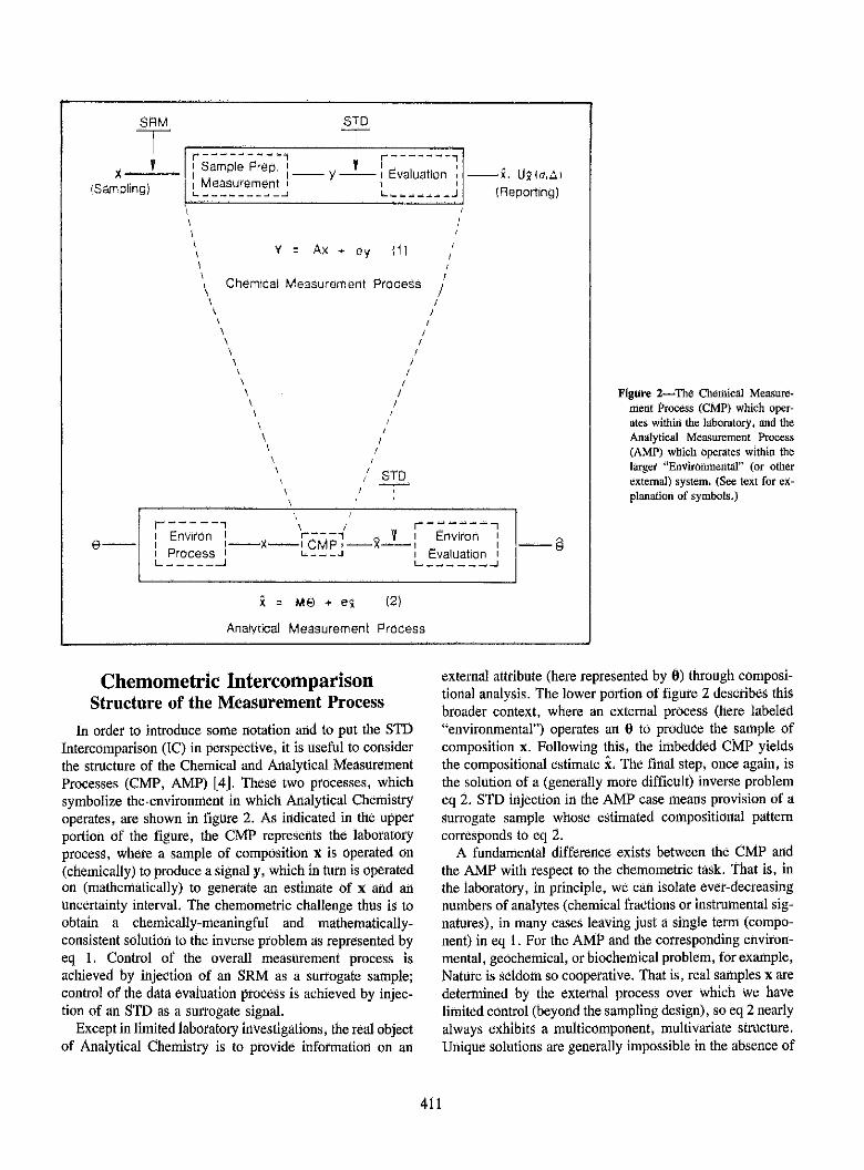
Figure 2-The Chemical Measure-ment Process (CMP) which oper-ates within the laboratory, and theAnalytical Measurement Process(AMP) which operates within thelarger "Enviromrental" (or otherexternal) system. (See text for ex-planation of symbols.)

Chemnometric IntercomparisonStructure of the Measurement Process

In order to introduce some notation and to put the STDIntercomparison (IC) in perspective, it is useful to considerthe structure of the Chemical and Analytical MeasurementProcesses (CMP, AMP) [4]. These two processes, whichsymbolize the environment in which Analytical Chemistryoperates, are shown in figure 2. As indicated in the upperportion of the figure, the CMP represents the laboratoryprocess, where a sample of composition x is operated on(chemically) to produce a signal y, which in turn is operatedon (mathematically) to generate an estimate of x and anuncertainty interval. The chemometric challenge thus is toobtain a chemically-meaningful and mathematically-consistent solution to the inverse problem as represented byeq 1. Control of the overall measurement process isachieved by injection of an SRM as a surrogate sample;control of the data evaluation process is achieved by injec-tion of an STD as a surrogate signal.

Except in limited laboratory investigations, the real objectof Analytical Chemistry is to provide information on an

external attribute (here represented by 0) through composi-tional analysis. The lower portion of figure 2 describes thisbroader context, where an external process (here labeled"environmental") operates an 0 to produce the sample ofcomposition x. Following this, the imbedded CMP yieldsthe compositional estimate xi The final step, once again, isthe solution of a (generally more difficult) inverse problemeq 2. STD injection in the AMP case means provision of asurrogate sample whose estimated compositional patterncorresponds to eq 2.

A fundamental difference exists between the CMP andthe AMP with respect to the chemometric task. That is, inthe laboratory, in principle, we can isolate ever-decreasingnumbers of analytes (chemical fractions or instrumental sig-natures), in many cases leaving just a single term (compo-nent) in eq 1. For the AMP and the corresponding environ-mental, geochemical, or biochemical problem, for example,Nature is seldom so cooperative. That is, real samples x aredetermined by the external process over which we havelimited control (beyond the sampling design), so eq 2 nearlyalways exhibits a multicomponent, multivariate structure.Unique solutions are generally impossible in the absence of

411

scientific knowledge concerning the external ("environ-mental") system.

The following STD intercomparison consists of univari-ate data (y) from a simulated CMP. The second exampleconsists of multivariate data (i) from a simulated AMP.Both ICs took place because of analytical measurementproblems having major public import-the first related toaccurate monitoring of radioactivity; the second, to accurateapportionment of atmospheric pollutants.

STD Vector-IAEA Intercomparison

of Gamma Ray Spectrum Analyses

In connection with their Analytical Quality Control Ser-vices program, the International Atomic Energy Agency(IAEA) undertook in 1976-77 a broad interlaboratory dataevaluation exercise involving computer-simulated high res-olution Ge(Li) gamma ray spectra such as might arise incontemporary neutron activation analysis [7]. The purposeof the intercomparison was both to assess the state of the-y-spectrum evaluation art and to provide data sets of knownstructure to assist in the improvement of that "art" (or sci-ence?). To my knowledge this was the first numericalchemometric intercomparison of such scope, using STDvectors. The organization and structure of the IAEA exer-cise are summarized in table 2.

Several features of the IAEA intercomparison wereanalogous to those involving chemical measurement inter-comparisons with reference materials. First, the STD werewell-characterized, with y-rays of known identity (energy)and amplitude. The "samples" were absolutely homogenous(identical numerical data to all participants), and they simu-lated observations from actual laboratory samples. SRM

intercomparison organizers strive to also meet such condi-tions, but of course they can only approach the homogeneityand exact composition knowledge found with STD. TheIAEA data sets also had known random error distributions(Poisson), a situation which is actually approached in manynuclear experiments, but which can never be guaranteed.Realism was preserved in the shapes of the y-peaks, in thatthey were derived from high precision observations withGe(Li) spectrometers. The fact that these shapes were notanalytic was one of the more discriminating elements of theIC, particularly for the resolution of doublets, where alter-native analytic or empirical peak shape functions had to beemployed [8]. (Each peak was approximately Gaussian nearthe top but decidely asymmetric near its base.) Referringagain to table 2, we can see that important planning tookplace, over a three-year period, resulting in four categoriesof data designed to provide initial "calibration," and to testdetection, accuracy and precision in quantification, anddoublet resolution. The importance of the pilot study cannotbe overstated; development of realistic STD of sufficient butnot excessive complexity does not come about without care-ful initial trials and iteration.

Detailed results for the IC may be found in [7]. Some ofthe highlights follow. Figure 3, for example, shows thespectrum (pattern) offered the participants, in digital andanalog form, to address the problem of unknown peak detec-tion. Participants knew only the calibration peak shape (asa function of "energy" or channel number) from the Refer-ence Spectrum #100 (not shown), plus the facts that theunknown peaks were singlets and that random errors werePoisson. The numbers and locations of the trace peaks wereto be determined. (The steep rise in the baseline near thecenter of the spectrum was inserted by the IAEA to simulatea Compton Edge.) The inset shown in figure 3 gives some

Table 2. Structure of the IAEA Gamma-Ray STD intercomparison.

Objectives

* To permit each participant to assess the accuracy of his data evaluation process.* To determine the quality of alternative gamma-ray spectrum evaluation methods as applied in representative laboratories.

Evolution

* 1973: Proposed at Consultants Meeting.* 1975-6: Pilot Study involving a small number of experts.* 1976-7: Full IC, involving 163 labs in 34 member states.* Currently: Simulation data offered as continuing pan of the IAEA Analytical Quality Control Service.

Data Sets

* Reference Spectrum: 20 high-precision peaks spanning 2000 channels.* Detection Spectrum: 22 subliminal peaks, whose number and locations were unknown to participants; detection criteria (a-, P-errors) were left

to individual judgment.* Precision Spectra: 6 replicate spectra having 20 known plus 2 unknown, large singlet peaks (Poisson statistics).* Resolution Spectrum: 9 doublets of unknown location and relative amplitude.

412

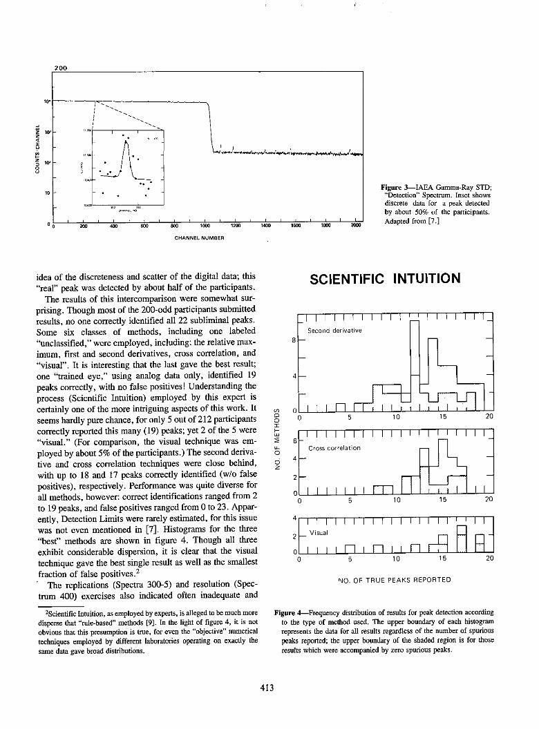
Figure 3-IAEA Gamma-Ray STD;"Detection" Spectnum. Inset showsdiscrete data for a peak detectedby about 50% of the participants.

Adapted from [7.]

idea of the discreteness and scatter of the digital data; this

"real" peak was detected by about half of the participants.

The results of this intercomparison were somewhat sur-

prising. Though most of the 200-odd participants submittedresults, no one correctly identified all 22 subliminal peaks.

Some six classes of methods, including one labeled

"unclassified," were employed, including: the relative max-

imum, first and second derivatives, cross correlation, and

"visual". It is interesting that the last gave the best result;

one "trained eye," using analog data only, identified 19

peaks correctly, with no false positives! Understanding the

process (Scientific Intuition) employed by this expert is

certainly one of the more intriguing aspects of this work. It

seems hardly pure chance, for only 5 out of 212 participants

correctly reported this many (19) peaks; yet 2 of the 5 were

"visual." (For comparison, the visual technique was em-

ployed by about 5% of the participants.) The second deriva-

tive and cross correlation techniques were close behind,

with up to 18 and 17 peaks correctly identified (w/o falsepositives), respectively. Performance was quite diverse forall methods, however: correct identifications ranged from 2

to 19 peaks, and false positives ranged from 0 to 23. Appar-

ently, Detection Limits were rarely estimated, for this issue

was not even mentioned in [7]. Histograms for the three

"best" methods are shown in figure 4. Though all three

exhibit considerable dispersion, it is clear that the visual

technique gave the best single result as well as the smallest

fraction of false positives. 2

The replications (Spectra 300-5) and resolution (Spec-trum 400) exercises also indicated often inadequate and

2 Scientific Intuition, as employed by experts, is alleged to be much moredisperse that "rule-based" methods [9]. In the light of figure 4, it is notobvious that this presumption is true, for even the "objective" numericaltechniques employed by different laboratories operating on exactly the

same data gave broad distributions.

SCIENTIFIC INTUITION

8

0

6

4

0,:r

:5nb'sI-uj

LLi

2

0

A

6 1 I I I I I I I I I I I I I I I I I I 1_cross correlation

0 IIIII1l IIIlII 11j0 5 10 16 20

0 5 10 15 20

NO. OF TRUE PEAKS REPORTED

Figure 4-Frequency distribution of results for peak detection accordingto the type of method used. The upper boundary of each histogramrepresents the data for all results regardless of the number of spurious

peaks reported; the upper boundary of the shaded region is for those

results which were accompanied by zero spurious peaks.

413

2

Iu

0

CHANNEL NUMBER

0 5 10 15 20

I I I I I I I I I I I I I I I Visual

20vin

widely varying performance. The majority of the resultssubmitted contained quite inaccurate or no estimates of un-certainty for large singlet peaks, even though the randomerror distribution was known; and less than 25% of theparticipants even submitted results for the most difficultdoublet resolution case.

The IAEA Simulation Data Sets have been viewed ofsufficient importance that they have become an integral partof the Intercomparison Programme of the Analytical QualityControl Service of that organization. The most recent offer-ing was issued in December 1984 [10] where STD Drayspectra are included alongside isotopic and trace elementIntercomparison and Certified Reference Materials of im-portance in many areas of nuclear and environmental analy-sis.STD Matrix-NBS-EPA Intercomparison of Source Ap-portionment Techniques. The second case study com-prises STD in the form of two-dimensional data matrices,simulating sets of atmospheric aerosol samples each ana-lyzed for up to 20 chemical species [11]. The stimulus forthis exercise, which is believed to be the first STD intercom-parison involving Data Matrices, was the great potential butgreat difficulty of identifying multiple pollutant sources viatheir "chemical fingerprints" as preserved in ambient parti-cles, (A vivid illustration adjoins [11], where one findsdiscord even in assigning names to pollutant factors deducedfrom elemental patterns observed in actual measurements of[Houston] aerosol samples [12].) As noted at the beginningof this section, this type of problem is characteristic of theAMP, where superposition of multiple components is intrin-sic to the nature of the system, so chemical manipulationcannot simplify the structure of eq (2).

We designed the STD in coordination with (nearly) all ofthe "Receptor Modeling" (source apportionment) experts inthe U.S. with the object of providing a few realistic datamatrices covering a range of problems. The overall structureof the study is given in table 3. The data matrix x is givenby the superposition of source contributions (MO)j, whereeach source has a characteristic chemical pattern or profileMi and a temporal (or spatial) intensity pattern Oj Threeclasses of error typify such measurements, as indicated inthe table. A significant task involved building the databaseof source profiles and error terms. Unlike the y-ray calibra-tion profiles (peak shapes), the aerosol source profiles werenot even approximately analytic (fig. 5, top); reliable empir-ical field data had to be sought and evaluated.

When generating data matrix STDs, one must pay atten-tion to a major new element of complexity which is absentfrom data vector STDs. That is, unless the simulation dataare to be no more than arbitrary superpositions of sourceswith added random errors, it is essential to generate thesource intensity patterns by means of suitable source emis-sion locations (emissions inventory map) plus realistic mix-ing and transport to the receptor (sampling) site(s). This stepis intrinsic to the nature of the data matrix; it underlies itsmultivariate character, and it highlights information (sourcemap, meteorological patterns...) external to the datamatrix, per se, which may be crucial for a successful dataanalysis. The source map used for the simplest of our threedata sets is shown in the lower portion of figure 5. Stochas-tic source impacts at the receptor R were generated bybringing together the source map, emissions intensities andoperating schedules, actual meteorological data (from St.Louis, September 1976), and the 'RAM' atmospheric dis-

Table 3. Structure of the source apportionment simulation test data.

Generating equation

P

ii,=L [M-ea,+el]Hynl +eu

where:

p = number of active sources (p - 13)t=sampling period (l-tG 40)

x,="obscrved" concentration of species i for period t (T1_i6,ANI20)j, =true intensity (at receptor) of source j(lqjlp)

M1 }='observed' source profile matrix (element j1)ei =random niaesurenlent errors, independent and normally distributede,1 1=systenotic source profile errors, independent and normally distributed (systematic because fixed over the 40 sampling periods)c=ranhdom source profile variation errors, independent and log-normally distributed

Data set characteristics

Set l: p=9 (including one unknown source)* enrors=el, em: City Plan No. I (fig. 5)Set 11: p= I (all known); errors =eI,e,,; City Plan No. 2Set III: p = 13 (all known); errors=ei, em. eH; City Plan No. 2

-For DOat Set I, participants were told only that pl-3.

414

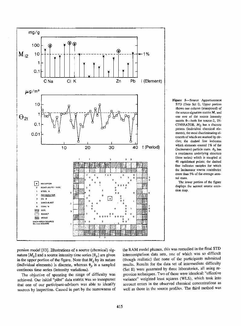
jyl i ( 3'CNa CI K Zn Pb i (Element)

10 _

0.01 _

isREC~tYOHO ROAO AUTO . SOIL

1 STEEL A

2 INCINEtMATOR

OIL S

4 SAN.BLASt

S CO AL S

[3 BASAitWOOD

EACH AREA SOURcEIS s N= SoUAnE

10 20 30

0 0

40 t (Period)

E Io

o ., .' /

0

ax2

;I

I//a.

Figure 5-Source ApportionmentSTD (Data Set 1), Upper portionshows one column (transposed) ofthe source signature matrix M, andone row of the source intensitymatrix 0-both for source-2, IN-CINERATOR. Mi2 has a discretepattern (individual chemical ele-ments), the most discriminating el-ements of which are marked by cir-cles; the dashed line indicateswhich elements exceed 1% of the(Incinerator) particle mass. 02, hasa continuous underlying structure(time series) which is sampled at40 equidistant points; the dashedline indicates samples for whichthe Incinerator source contributesmore than 5% of the average aero-sol mass.

The lower portion of the figuredisplays the aerosol source emds-sion map.

persion model [13]. Illustrations of a source (chemical) sig-

nature [M1 ] and a source intensity time series [0jI] are given

in the upper portion of the figure. Note that M 4j by its nature

(individual elements) is discrete, whereas %j, is a sampled

continous time series (intensity variations).The objective of spanning the range of difficulty was

achieved. Our initial "pilot" data matrix was so transparentthat one of our participant-advisors was able to identifysources by inspection. Caused in part by the narrowness of

the RAM model plumes, this was remedied in the final STDintercomparison data sets, one of which was so difficult

(though realistic) that none of the participants submittedresults. Results for the data set of intermediate difficulty(Set 11) were generated by three laboratories, all using re-gression techniques. Two of these were identical: "effectivevariance" weighted least squares (WLS), which took into

account errors in the observed chemical concentrations aswell as those in the source profiles. The third method was

415

mg/g

100

Mi2 10

1

0.1

ridge regression, of interest because of the high degree ofcollinearity among the 13 sources. For the most part, thethree sets of resuits were self consistent, and within a factorof 2 of the truth. For four of the sources, however, widelydiscrepant results were reported-a surprising outcome, forsimilar or identical numerical methods were applied to iden-tcal numerical data.

An exploratory graphical analysis of the results from thetwo laboratories using weighted least squares (WLS-1, -2)is shown in figure 6. This approach, which was inspired bythe "Youden Diagram" for bi-rmaterial inrercomparisons,a4DwR us :o spot 'ouliiers"' from the line of concordance.(As with the line drawn for .:e Youden Ll ot of figure 1. the45° line in figure 6 was drawn independent of the data-i.e.,it was in no way "fitted".) Exact results would fall at theorigin (0. 0), and equivalent data reduction bv the twolaboratories would prodLce results lying or: the line. Disper-sion along the line derives from random enrors bLiit into thecommon data set and systematic errors connected with thecommon numerical model (WLS). Two of the sources (Ag,0,) were well below their detection limits, and will not befurther discussed here. The three outlices (Cf point 'x' in

1O.0

r-

-C

El4-

5-

'IZ:

LU

1.0 _

0.1 1

0.01 -

0.01 0.1 1.0 10.0

Standard Error (pg/m3)

Figure 7-Absolute errors ror each or the 13 source estimates for Data SetIi, byWLS-1 ix), WLS-2(+) iand Ridge Regression (i), plotted as afunction of the reported stucdard errerss. (On the average about 213 of thepoints for a correct method should fall below the diagonat.)

SJ - PLOT (Dale Seil I)

4aC-

200-

zoo_

e -100 _ ----- _____-----____S

0

Z.50 C,2~~~~~~~CC, ,I/

--5J -

1IcC

I r I

a, f ,

-50 0 so i0o 20o

Percent Oeinw ,VLS-1l

Figure 6-"Scientific Judgment" Plot. Correlation (Youden-type) Dia-gram showing data evaluation resuts of laboraturry-2 vs laboslery-loperatine on the same data set (iI) using the same method of numericalanalysis (weighted Least Squares). Deviations from the non-fitted tineof concordance imply chemometric 'operator erior" (SJ).

[Source Codes: Steel-A (8,), Steel-B (S2), Oil-A (of Oil-B (02),Incinerator (1), Class Nffr (G), Coal-A (Cl), Coal-B (C2), Aggregate

(Ag), Basalt (B), Soil (So), Auto (v). Wood Smoke (W)j

Figure I-G , W. and Cl-deserve oar attmntior. however.As will be shown rin the next section, shby may be attributedto what the laboratories involved labeled "Scientific Judg-ment." Discovering this factor, and understanding its na-tzre, was one of the unexpected but important outcomes ofthe experiment.

Another major difference and inadequacy among the lab-oratories relates to the uncertainties (i.e., SEs) reported. Alldid report standard errors, but an examination of the actualdeviations from the truth for the 13 estimates from each labwas illuminating. For one of the three, all 13 (absolute)deviations exceeded the SEs by factors of 2 to 10, whereasfor another lab the deviations were all straller than. the SEsby fattes of ahctfl 1.6 to 30. None cf the Abs -enrtzdlxLnd5 for sylemnatic or mozel m LUI . (See fi . 7..

Because of Ile rnultvariat- cuanacte-cf the sorsceappor-tionment data sets, both simple linear regression and factoranalysis (FA) techniques could be applied. The regressionmethods ("Chemical Mass Balance", i.e., WLS) were themore precise, when model information and source profileswere available. When the model was not fully known and ifthe number of interfering components was not too great,factor analysis or certain hybrid methods appeared to yieldmore acceptable results. Such was the case for Data Set I%vhi'ch had 9 sourzes, one of which was unknown to theparticipants. In Set 11, however, with 13 known sourceshaving a significant degree of multicollinearity, factor anal-ysis was able to discern but four sources.

416

iI

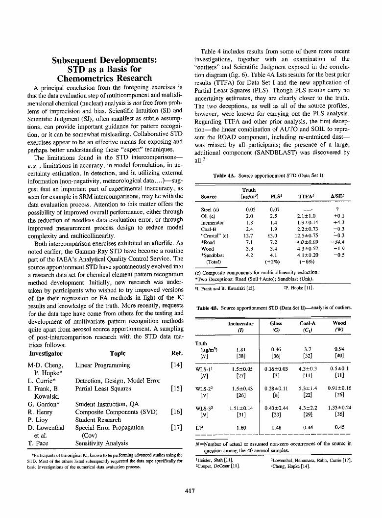
Subsequent Developments:STD as a Basis for

Chemometrics ResearchA principal conclusion from the foregoing exercises is

that the data evaluation step of multicomponent and multidi-

mensional chemical (nuclear) analysis is not free from prob-

lems of imprecision and bias. Scientific Intuition (SI) and

Scientific Judgment (SJ), often manifest as subtle assump-tions, can provide important guidance for pattern recogni-tion, or it can be somewhat misleading. Collaborative STDexercises appear to be an effective means for exposing and

perhaps better understanding these "expert" techniques.The limitations found in the STD intercomparisons-

e.g. , limitations in accuracy, in model formulation, in un-certainty estimation, in detection, and in utilizing externalinformation (non-negativity, meteorological data,. ..)-sug-gest that an important part of experimental inaccuracy, asseen for example in SRM intercomparisons, may lie with the

data evaluation process. Attention to this matter offers thepossibility of improved overall performance, either throughthe reduction of needless data evaluation error, or throughimproved measurement process design to reduce modelcomplexity and multicollinearity.

Both intercomparison exercises exhibited an afterlife. Asnoted earlier, the Gamma-Ray STD have become a routine

part of the IAEA's Analytical Quality Control Service. Thesource apportionment STD have spontaneously evolved intoa research data set for chemical element pattern recognitionmethod development. Initially, new research was under-taken by participants who wished to try improved versionsof the their regression or FA methods in light of the ICresults and knowledge of the truth. More recently, requestsfor the data tape have come from others for the testing anddevelopment of multivariate pattern recognition methodsquite apart from aerosol source apportionment. A samplingof post-intercomparison research with the STD data ma-trices follows:

Investigator

M-D. Cheng,P. Hopke*

L. Currie*1. Frank, B.

KowalskiG. Gordon*R. HenryP. LioyD. Lowenthal

et al.T. Pace

Topic

Linear Programming

Detection, Design, Model ErrorPartial Least Squares

Student Instruction, QAComposite Components (SVD)Student ResearchSpecial Error Propagation

(Cov)Sensitivity Analysis

Ref.

[14]

Table 4 includes results from some of these more recent

investigations, together with an examination of the"outliers" and Scientific Judgment exposed in the correla-don diagram (fig. 6). Table 4A lists results for the best priorresults (TTFA) for Data Set I and the new application ofPartial Least Squares (PLS). Though PLS results carry nouncertainty estimates, they are clearly closer to the truth.The two deceptions, as well as all of the source profiles,however, were known for carrying out the PLS analysis.

Regarding TTFA and other prior analysis, the first decep-tion-the linear combination of AUTO and SOIL to repre-sent the ROAD component, including re-entrained dust-was missed by all participants; the presence of a large,additional component (SANDBLAST) was discovered byall.'

Table 4A. Source apportionment STD (Data Set 1).

TruthSource [tg/rn3 ] PLSI TTFA 2 A/SE2

Steel (c) 0.05 0,07 --- ?

Oil (c) 2.0 2.5 2.1±1.0 +0.1Incinerator 1.3 1.4 1.9±0.14 +4.3Coal-B 2.4 1.9 2.2±0.73 -0.3"Crustal" (cl 12.7 13.0 12.5±0.75 -0.3*Road 7.1 7.2 4.0 ±0.09 -34.4Wood 3.3 3.4 4.3±0.52 +1.9

*Sandblast 4.2 4.1 4. I±0.20 -0.5(Total) (+2%) (-6%)

(c) Composite components for multicollinearity reduction.*Two Deceptions: Road (Soil+Auto); Sandblast (fUnk).

t. Frank and B. Kowalski [15] 2pf Hopke [11T.

Table 414. Source apportionment STD (Data Set I)-analysis of outliers.

Incinerator Glass Coal-A Wood(I) (G) (Cd (W)

Truth(ALg m3 ) 1.81 0.46 3.7 0.94[N] [38] [36] [32] [40]__________ _____________

WLS-15

[N]

[15] WLS-22

[N]

1.5±0.05[27]

1.5±0.43[26]

WLS-33 151±0.14[16] [NV] [31]

[171 LI4 1.60

0.16±0.03 4.3±0.3 0.5±0.1[3] [II] [11]

0.28±0.11 5.3±t1.4 0.91±0.16[8] [22] [26]

0.43±0.44 4.3±2.2 1.33±0.24[231 [29] [36]

0.48 0.44 0.45

N=Number of actual or assumed non-zero occurrences of the source inquestion among the 40 aerosol samples.

tHeisler, Slah [II].2Cooper. DeCesar [11].

3Lowenthal, Hanumraa, Rahn, Currie [17].4Cheng, Hopke [14].

417

Participants of the original IC, known to be poramsisg advanced studies using theSTD. Most of the others listed subsequently requested the data tape specifically forbasic investigations of the numerical data evaluation process.

The outliers (G, Ct, W) from data Set 11 are examined intable 4B for new and earlier analyses. The INCINERATORresults, which fell directly on the line of concordance (fig.6), are included for comparison. It is interesting that Lllinear programming gave significantly improved results forsources I and G, but much poorer results for the other twosources. A conjecture, which bears investigation, is that inthe absence of experimental blunders, least absolute residu-als carry too high a penalty in highly collinear problems. Wegain some understanding of Scientific Judgment (SJ) fromthe three WLS results. It is apparent that the exercise of SJin deleting rare components from the model is operator-dependent and generates important differences in overallresults. This is an issue deserving additional research, theoutcome of which could be the transformation of Ad-Hoc SIinto scientifically-based SL4

ConclusionFor modern Analytical Chemistry, where chemometric

approaches are mandatory to resolve complex signals frommultianalyte mixtures, Simulation Test Data serve two im-portant purposes: 1) The assessment of interlaboratory data-evaluation precision and accuracy; and 2) the exposure of SIand SJ plus the generation of more powerful methods ofcombining scientific knowledge with advanced techniquesof data analysis. The need for this is critical, because inprinciple nearly all of our multicomponent "inverse" prob-lems are underdetermined-i.e., solutions cannot obtain inthe absence of explicit (or hidden) assumptions. We con-clude with a summary of recommendations for the prepara-tion of STD data sets, and open research questions whichcould be fruitfully addressed by chemometricians (table 5).

Table 5. STD exercises,

Observations and Recommendations

* Benefits: Controlled model, errors; Truth is known.* Prerequisites: defined objectives, 'lab' population, plan, input datamodel.* Pilot study advisable.* Investigate 'surprises-unexpected accuracy, discrepancies.* Blind; anonymous; don't score; discourage premature communication.* Deceptions: mimic reality; be not too obvious.

Some Open Questions

* Adequate treatment of uncertainty-esp. bias (bounds).* Further understanding of 'SI' and 'SI'-who are the experts?* Utilization of external information: phenomena, data, "fuzzy" S& partial knowledge, constraints,...* Treatment of the 'total' problem (simultaneous estimation over the entire data matrix), mdn. errors in y' and 'A'.* Solution and uncertainties when the linear model doesn't apply (physical-chemical and mathematical strategies; eg, atmospheric transformation).

Special recognition should be given to the designers of thetwo STD exercises discussed, as well as to the participantsand the scientists who are using the STD for continued basicresearch in chemometrics. R.M. Parr (IAEA - STD) andR.W. Gerlach (Source Apportionment - STD) made essen-tial contributions. Others deserving special recognition arelisted as authors of references [7, 11], and [14 - 18].

3STD deceptions-i.e., realistic complications-are, of course. in orderfor all but the simplest of exercises. Though organizers should attempt tospan the range of difficulty occurring with real data sets, they should notdo so in too obvious or regular a manner. Informing the IAEA y-ray STDparticipants, for example, that the multiplets had just 2 components wasalready a considerable simplification, but the regular spacing (1, 3, 10channels) and relative amplitude (1, 3, 10) of the doublet members wasunnatural and could encourage a certain amount of guess work on the partof the participants.

4The paradigm proposed here classifies experts' decisions or assump-tioas as "intuitive" (SI) or "judgmental" (SJ) depending on whether they arebased on sound (though possibly subliminal) reasoning or ad hoc judg-nments, respectively. These asymptotic classes may each yield correct orincorrect results, just as target and contaminating populations may eachproduce outliers or inliers. though with differing probabilities.

References[1] Eisenhart, C., Science 160 (1968) 1201.[2] Currie, L.A., and JRi Devoe, Chapt 3 in JR. DeVoe, Ed. VALI-

DATION OF THE MEASUREMENT PROCESS, Amer ChemSoc Sympos Ser #63 (1977).

[3] Youden, W.I., Anal Chem 32 [13] (1960) 23A.[4] Currie. L.A., Pure & App! Chem, 54 (1982) 715.[5] Lamuparski, L.L., and T.J. Nestrick, Anal Chem, 52 (1980) 2045.[6] Kirchhoff, W.H., Edit, NBSIR 82-2511 (1982).[7] Parr, R.M.; H. Houtermans, and K. Schaerf in COMPUTERS IN

ACTIVATION ANALYSIS AND GAMMA-RAY SPEC-TROSCOPY, US Dept of Energy, CONF-780421 (1979) 544.(See also Zagyvai, P.; R.M. Parr and L.G. Nagy, J. Radioanal.Nucl. Chem. 89 589 (1985).)

[8] Ritter, G.L., and L.A. Currie, ibid, p. 39.[9] Nalimov, V.V., FACES OF SCIENCE, ISI Press (Philadelphia,

1981).[10] IAEA Analytical Quality Control Service Program, LAB/243 (1984).[11] Curie, L.A.; R.W. Gerlach, C.W. Lewis, W.D. Balfour, L.A.

Cooper, S.L. Datuner. R.T. DeCesar, G.E. Gordon, S.L. Heisler,P.K. Hopke, J.J. Shah, G.D. Thurston, and H.J. Williamson,Atm Environ 18 (1984) 1517.

[12] Dzubay, T.G.; R.K. Stevens, W.D. Balfour, H.J. Williamson, J.A.Cooper, I.E. Core, R.T. DeCesar, E.R. Crutcher, S.L. Datnner,

418

B.L. Davis, SL. Heisler, J.J. Shah, PI'K. Hopke, and D.L.Johnson, Atm Environ 18 (1984) 1555.

[13] Novak, J.H., and D.B. Turner, J. Air Ponut. Control Assoc., 26(1976) 570.

[14] Cheng, M-D., and P.K, Hopke, An Intercomparison of Linear Pro-gramming Procedures for Aerosol Mass Apportionment, Air Pol-lution Control Association Paper No. 85-21.8 (1985),

[15] Frank, I.E._ and .R. Kowalski, Statistical Receptor Models Solvedby Partial Least Squares, ACS Diva of Environ Chem Sympos

DISCUSSIONof the L.A. Currie paper, The Limitations ofModels and Measurements as Revealed ThroughChemometric Intercomparison

Leon Jay GleserDepartment of StatisticsPurdue University

The construction and use of Simulation Test Data (STD)to help evaluate alternative chemometric methodologies is ahighly welcome contribution to the field. Dr. Currie, and theagencies and colleagues whom he credits, are to be congrat-ulated for an approach which has the potential to promoteimprovements in the art of quantitative chemical analysis.

What follows is a brief discussion of some previous useof standard data sets in statistical research, along with somewarnings about the possible pitfalls connected with the useof such approaches. In particular, the parallel that Dr. Curriedraws between the use of standard data sets and interlabora-tory comparisons using common reference materials cannotbe pushed too far. Many interacting factors lead to bias inmodeling and analysis of complex data sets; the contribu-tions of these factors would be confounded in typical inter-laboratory comparison designs. One factor, scientific judg-

Abstracts (Philadelphia, Aug 1984) p. 202,[16] Henry, R.C.,Proc Air Pollut Control Assoc Spec Conf, SP-48 (1982J

141,[17] Lowenthal, DOH. RC. Hanumara, KA. Rahn, and L.A. Currie,

Estimates and Uncertainties in Chemical Mass Balance Appor-tionments: Quail Roost 11 Revisited, prepared for submission toAtmospheric Environment (1985).

[18] Stevens, R.K, and T.G, Pace, Atmos. Environ. 18 (1984) 1499.

ment, cannot even be identified in standard frequentistreports of statistical data analysis. This suggests that subjec-tive scientific judgments need to be given more explicitmention in reports of statistical analyses, perhaps throughthe use of the Bayesian approach to inference.

To make standard data sets more closely resemble real-world data, the use of the "bootstrap" is suggested. The"bootstrap" can also help in providing the estimates of statis-tical precision that Dr. Currie notes were lacking in the twostudies conducted to date.

Standard Data Sets in Statistics

Statisticians have long recognized the usefulness of hav-ing common data sets on which new methodologies can betried out, and their relative merits assessed. For example,

419

new methodologies for classification and discriminant anal-ysis are often applied to the iris data of E. Anderson [11',which was featured in a famous paper by R. A. Fisher [2].(To Anderson's undoubted frustration, these data are usu-ally referred to as "Fisher's iris data.")

Another famous data set is Longley's [3] econometriclinear regression data. In these data, the independent vari-ables in the regression are highly interrelated (multicolin-ear). Longley ran the data through several computer soft-ware packages designed to do least squares analysis. Intheory, all of these programs solve the same set of linearequations to estimate the regression slopes. However, thesolutions obtained by the various algorithms differed, insome cases even by sign! What had happened was that themulticollinearity in the data made the answers obtainedhighly sensitive to roundoff and truncation of the data, andthe algorithms differed by where and by how much roundoffs

were done. Longley's paper had the very beneficial conse-quence that software developers now pay careful attention tonumerical analysis in designing statistical algorithms. Fur-ther, it stimulated study of the resistance of statisticalmethodology to data perturbations (robustness).

However, Longley's paper (and particularly his data) mayalso have had a less salutory effect on software develop-ment. Software developers now know that consumers willtest out their programs on Longley's data. [See, for exam-ple, Lachenbruch's review [4] of STAN, Version 11.0 byDavid Allen.] This may lead them to overcompensate formulticollinearity problems, and consequently overlook orneglect other potential problems or sacrifice desirable fea-tures to include subroutines necessary to accurately processmulticollinear data.

This last comment points out a real danger in the use ofstandard data sets, namely that their existence can bias thedirection which development of methodology and softwaretakes. The best guard against such bias is the creation ofstandard data sets of many types.

An artificial standard data set (simulated according to aknown model for the distribution of errors) can lead to aparticularly serious bias. Chemometricians who know thattheir work will be evaluated by such data sets will tend touse a methodology which is known to be efficient for thegiven statistical model. Such a methodology, however, maynot do well against real data, for which the given statisticalmodel is not necessarily a good approximation. Alterna-tively, chemometricians may object to evaluations on thebasis of such data, arguing (with considerable merit) thatsuch data do not reflect their practical experience.

The reason, of course, for using artificial data is that the"truth" or "signal" underlying the "noise" (error) in the datais known. This allows us to separate bias (lack of validity)from precision (reliability, repeatability). In this respect

there is an obvious parallel, which Dr. Currie correctlypoints out, with the use of common reference materials ininterlaboratory comparisons. The goal of such studies is toeliminate bias (which is usually reflected in interlaboratoryvariation), and to estimate precision (intralaboratory varia-tion). However, whereas common reference materials are"real" (although they may be ideal examples of materialsanalyzed in practice), this is not clearly the case with datasimulated from specified statistical populations (e.g., Gaus-sian populations). Real populations may have "heavy tails"and/or other funny features (e.g., several modes) which arenot modeled by standard distributions.

One obvious solution is to vary the distributional assump-tions which generate the errors in artificial data. This ap-proach is widely used in statistics to study the robustnessproperties of statistical methodologies.

Another possible solution is to use the ideas underlyingthe "bootstrap" (Efron [5], Diaconis and Efron [6], Freed-man and Peters [7,8]) to simulate data which have "realworld" error distributions.

The Bootstrap

In using the "bootstrap," we start by assuming that theobserved data yi are related to unknown parameters 6 anderrors ei by a model

yi =G(Oen), i = 1,2,...,n, (1)

where G(-,') is known. Given a value for 6 (which may bea vector), we assume that the eq (1) can be inverted to obtainthe errors ei. That is,

e, =Hi(0,y 1 ,. .. y,,), i=l.. (2)

Given "real" data yI' Y2. .Y,,. with n sufficiently large togive us some hope of accurately estimating 6 by

w =h yls (smeY d),

we now construct the residuals (estimated errors)

i=l1,2,...,n. (3)

The resulting finite population {( ,...,J} of residuals is thestatistical population from which we can randomly samplenew errors ei, i = 1,2,...,,n, to create standard data sets

yi =G (0*,Ze), i =1,2,...,m I

'Figures in brackets indicate literature references. where 0* can be chosen to have any desired value.

420

The data sets so simulated are not entirely "real." Themodel (I) relating observations yi to errors e, must still bespecified, and need not be correct. However, such modelscan be specified (and criticized) taking account of chemicaland physical theory, without also imposing statistical as-sumptions about distributions of errors. As such, these mod-els are "prestatistical."

A population of residuals &i that is too small can misrep-resent statistical variation. Thus, attempts should be made toconstantly enlarge this population with new residuals ob-tained from real data obtained in contexts described by themodel (1). Since the "bootstrap" is a fairly recent statisticaldevelopment, new insights into problems and advantagesconnected with the method are constantly being published.Consequently, the input of specialists in "bootstrap"methodology should be sought when applying this method

to the generation of standard data sets. In particular, changesin instrumentation, personnel, or experimental design maychange the error population over time. Careful attentionshould be paid to detect such shifts in distribution.

Not all measurement contexts lend themselves to the"bootstrap," since the transformation (2) from observationsto errors may not exist, or may not be well defined. (Thismay be the case, for example, with the Gamma Ray Spec-trum Analysis example discussed by Dr. Currie.) However,when the "bootstrap" does apply, it can be used both tocreate standard data sets, and also to provide nonparametricestimates of precision [5,7,8].

Estimates of Precision

Although I share Dr. Currie's concern that the laborato-ries in his two examples either failed to provide estimates ofprecision, or gave incorrect estimates, I must point out thatin Dr. Currie's two examples, it is not clear what measuresof precision are appropriate. In all of the analyses, multipledecisions are made. For example, in the Gamma-Ray exam-ples, the locations and amplitudes of several peaks had to bedetermined simultaneously. Although individual standarderrors can be given, these do not directly provide measuresof simultaneous accuracy [9]. Further in the detection spec-trum and precision spectra sets, even the number of peakswas unknown. This produces a highly complicated estima-tion problem for which only large-sample approximations toprecision are available. There is some evidence in the liter-ature that such large-sample approximations have consider-able bias in moderate samples (see, e.g., [6]).

Similar problems arise in the three data sets for the NBS-EPA Source Apportionment study, particularly in the caseof Data Set 1, where the number of sources is left unspeci-fied. Both ridge regression and factor analysis are ex-ploratory methodologies, requiring iteration and judgmentthat are difficult to describe analytically. The only available

measures of precison for such techniques are large-sampleapproximations which refer to analytical formulas for theestimators not directly related to the way such estimators areactually obtained. For example, I know of no way to specifythe precision of estimates of slope obtained by the ridgetrace method. Published formulas for the precisions of ridgeregression estimators refer to those estimators in which theridge factor k is a specified function of the data, rather thanbeing obtained by inspection of the ridge trace.

Given the complex natures of the estimation problemsthat Dr. Currie describes, and the fact that statistical theoryhas not yet provided reasonable estimates of precision forsome of the methodologies used in these problems, it is notsurprising that the laboratories either failed to provide mea-sures of precision, or gave estimates that were off the mark.Clearly, there is much theoretical statistical work yet to be

done.In the meantime, it should be mentioned again that the

"bootstrap" can provide estimates of precison in cases wherethe assumptions (1), (2) underlying the bootstrap are appli-

cable.

Analogy to CMP InterlaboratoryComparisons

As already noted, Dr. Currie makes an analogy betweenthe use of standard data sets in the two examples he dis-cusses, and traditional interlaboratory comparisons usingcommon reference materials. However, this analogy cannotbe carried too far, since there are some important differencesin context.

In traditional interlaboratory comparisons, differencesbetween laboratories are usually assumed to be due to vari-ations in the calibration (adjustment) of the instruments, orto differences in instrumentation or technique. Conse-quently, a one factor (additive) components of varianceANOVA model can reasonably be employed to assign vari-ability between inter- and intra-laboratory sources.

In the standard data set context described by Dr. Currie,however, there are at least three factors which can describevariability between laboratories: I) different models or as-sumptions used, 2) different statistical methodologies em-ployed, and 3) different numerical algorithms. Further, the"levels" of these factors (particularly factor 1) appropriate todescribe a given laboratory's analysis are not always appar-ent. (Not all assumptions made are clearly stated). For ex-ample, "outliers" can be discarded, parameter values can betruncated (e.g., negative estimated amplitudes reported aszero), or several different analyses may be run but only one(the one that the laboratory thinks is "right") reported. Con-sequently, it will be difficult to separate sources of interlab-oratory variation.

Even worse, even if all factor levels can be accuratelyidentified (or set in advance), there is the clear possibility of

421

interaction among factors, making interpretation of resultsdifficult. For example, different methodologies work "best"in the context of different models, and different models andmethodologies lead to different algorithms and thus to dif-ferent reasons for numerical instability when such al-gorithms are applied to data.

How do we then interpret Dr. Currie's examples? First,and most important, we see that in certain far more preciselydefined contexts (in terms of model) than would be met inpractice there are wide variations in conclusions betweenlaboratories, and also wide variations from the correct an-swer. Second, the divergences between laboratories cannotbe assigned to sampling variation because (and this is thebeauty of the standard data sets) the data are fixed. How-ever, the divergence of the centroid of the laboratory conclu-sions from the truth may be due to sampling variation (thesample did not represent the population), or to poor labora-tory conclusion-making processes, or to both. We cannotpartition this last variability in terms of possible causes,because no accurate measures of precision over samplingvariation are provided by the laboratories, or (in some cases)known.

To better understand the sources of interlaboratory varia-tion, we need to start with pilot studies that control the levelsof each of the factors (1-3) listed above. To establish thecontribution of algorithms to interlaboratory variability, weneed to ask numerical analysts to study the possible numer-ical errors that can occur in algorithms, describe the situa-tions that produce these errors, and suggest remedies toreduce such errors. (Here, our "pilot sample" design fixesall factors but the "algorithm" factor.) To establish the con-tribution of methodology (or rather methodology - modelinteractions) to such variability, chemometricians (particu-larly statisticians) need to use mathematical analysis andsimulaton to identify formulas for the precisions (samplingvariability) that can be assigned to the various methodolo-gies in the contexts of various models (Here, we assume afixed, perfectly accurate algorithm, and vary combinationsof method and model.) Finally, we need to study and assessthe variability due to choice of model, and also to the other"scientific judgments" made by a laboratory in choosingmethodology and algorithms and in announcing measures ofprecision. It is particularly in this last type of study thatstandard data sets, both real and artificial, can be mostuseful.

proach. Scientific decision-making involves subjectivejudgments about both models and types of permissible con-clusions. When such judgments are unstated, we have seenthat this can obscure our understanding of how decisions arereached, and thus prevent us from finding sources of "bias"or error.

Bayesian statisticians, who try to mathematically modeltheir subjective judgments in terms of prior probabilitiesover unknown parameters (and models), are often accusedby frequentist statisticians of proposing analyses that lack"scientific objectivity." Clearly the contrary is true. Thescientist who claims to base conclusions only on the"objective" evidence provided by observed frequencies isnevertheless often guilty of imposing unstated judgments onsuch evidence. The Bayesian, at least, tries to bring thesejudgments into the open, where they can be assessed alongwith the data. Even if we doubt that probability models canever serve as adequate models of subjective belief, we canstill applaud the Bayesian's efforts to expose the methods bywhich this belief interacts with the evidence in the data toproduce new judgments or belief. Rather than criticize theBayesian for being "subjective" or "biased", the frequentistsneed to find ways of making their own decision-makingprocesses available for objective study, so that we can gainthe opportunity to learn how to improve scientific judgment.

References

[I] Anderson, E., The Irises of the Gaspe Peninsula. Bull. Amer. Iris Soc.59, 2-5 (1935).

[2] Fisher, R.A, The use of multiple measurements in taxonomic prob-lems. Ann. Eugen. 7, 179-188 (1936).

[3] Longley, JW., An appraisal of least squares programs for the elec-tronic computer from the point of view of use. Journ. Amer.Statist. Assoc. 62, 819-841 (1967).

[4] Lachenbruch, Peter A., Review of "STAN, Version 11.O." The Amer-ican Statistician 39, 146-148 (1985).

[5] Efron, B., The Jackknife, the Bootstrap and Other Resampling Plans,Soc. Indust. and Appl. Math.: Philadelphia, PA (1982).

[6] Diaconis, P., and B. Efron, Computer intensive methods in statistics.Scientific American, May, 116-130 (1983).

[7) Freedman, D.A., and S.C. Peters, Using the bootstrap to evaluateforecasting equations. Tech. Report, Dept. Statistics, U. Calif.Berkeley (1983).

[8] Freedman, D.A., and S.C. Peters, Bootstrapping a regression equa-tion: Some empirical results. Journ. Amer. Statist. Assoc. 79,97-106 (1984).

[9] Miller, R.G. Jr., Simultaneous Statistical Inference, 2nd edit.McGraw-Hill: NY (1981).

Scientific Judgment and Bayesian Inference

The question of how to analyze the biases introduced by"scientific judgment" has a direct relationship to a long-standing controversy between classical (frequentist) statisti-cians and those statisticians who advocate a Bayesian ap-

422

journal of Research of the National Bureau of StandardsVol. 90, No. 6, November-December 1985

Statistical Properties of a Procedurefor Analyzing Pulse Voltammetric Data

Thomas P. Lane

Massachusetts Institute of Technology, Cambridge, MA 02139

and

John J. O'Dea and Janet Osteryoung

State University of New York at Buffalo, Buffalo, NY 14214

Accepted: Jane 24, 1985

O'Dea et al. (1983, £ Phys. Chem. 97, 3911-3918) proposed an empirical procedure for obtaining estimatesand confidence intervals for kinetic parameters in a model for pulse voltammetric data. Their goal was to finda procedure that would run in real time, not necessarily one that would have well-defined statistical properties.In this paper we investigate some of the statistical properties of their procedure. We show that their estimationmethod is equivalent to maximum likelihood estimation, and their confidence intervals, while related to like-lihood ratio confidence regions, have a coverage probability that is not fixed and that is potentially quite large.We suggest modifications of their procedure that lead to more traditional confidence intervals. We examine theeffect on their procedure of the presence of nuisance paramters. Finally we discuss the possibility of seriallycorrelated errors.

Key words: autocorrelation; confidence intervals; estimation method; kinetic parameters; maximum likelihoodestimation; serially correlated errors; statistical properties.

1. Introduction

O'Dea et al. (1983) proposed a nonlinear regressionprocedure for estimating, and obtaining confidence in-tervals for, kinetic parameters describing the reductionof Zn(Il) at a stationary mercury electrode in aqueous

solutions of NaNO3 . In this paper we examine the statis-tical properties of the procedure and suggest mod-ifications to improve these properties.

In section 2 we describe O'Dea's procedure. In sec-tion 3 we show his estimation procedure to be equiv-alent to maximum likelihood estimation. In section 4 weshow his interval estimation procedure produces inter-vals that are related to higher-dimensional confidenceregions obtained by likelihood ratio theory, and we sug-gest modifications to the procedure that will produceconfidence intervals with the desired coverage proba-bility. In section 5 we question the assumption of

423

About the Authors: Thomas P. Lane is with theStatistics Center at MIT while John J. O'Dea andJanet Osteryoung are with the Department of Chem-istry at the State University of New York at Buffalo.

independent errors and examine the effect of includinganother parameter in the model to describe the apparentautoregressive error structure.

The notation used here is similar to that used byO'Dea, but as is customary in literature on regression weuse Y as the dependent variable.

2. Description of the Procedure

O'Dea models the observed response at time tj to anarbitrary pulse sequence by

Y,=af+c +Ei,

where a and c are unknown constants that convey nokinetic information, {EiJ is a sequence of errors that areassumed to be independent with mean 0 and unknownvariance o-2* The functionf=f(tj,a,k,E 4 ,) is the solutionof an integral equation. It depends on unknown kineticparameters a, k, and El, and it must be obtained bysolving the integral equation numerically.

The kinetic parameters are of primary interest, soO'Dea uses a nonlinear optimization procedure to findthe values of these parameters that maximize the cor-relation R between Yandf(t,a,k,EI,). These values aretaken as the estimates. Estimates of a and c can then beobtained by simple linear regression of Yonf(t,a,k,ET1),and a- can be estimated by the standard deviation of theresiduals from this regression.

With no error the correlation R calculated abovewould be equal to unity. O'Dea measures the deviationfrom unity by R = I -R and defines Rmj. as the optimumvalue of A?. To measure the uncertainty in his estimate ofa he fixes k and E. at their optimal values and finds thetwo values of a that give R = 3 Rj,,. He calls the intervalbetween these values a "confidence interval" for a, buthe assigns no confidence level to the interval. He com-putes similar intervals for k and Eb.

3. Maximum Likelihood Estimation

A more traditional approach to a problem of this sortwould be to write the likelihood or log likelihood func-tion for the problem and maximize it as a function of theunknown parameters. For normally distributed errorsthis is equivalent to choosing parameter values that min-imze the sum of squared residuals. In this section weshow that the above estimation procedure is also equiv-alent to maximum likelihood estimation.

If n is the number of observations, the log likelihoodL is given by

L(a~cakE,aro)= -n log(2TaO2) I Y-c -a ]2

The maximum is easily found by noting that for anyvalue of a-, the expression is maximized by choosing a,c, a, k, and E. to minimize the sum of squared residualsSSR=!(Y-c-aI) 2 . It is a simple matter to showthat if Y+n-'XYj and SST=2(Y-_y) 2 , thenSSR =(I -R )SSr, so SSR is a minimum when R is amaximum (in absolute value). Therefore O'Dea's esti-mates are the maximum likelihood estimates.

4. Confidence Intervals

Confidence regions for unknown parameters are oftenfound by computing the maximum likelihood estimatesand then finding other sets of parameter values forwhich the likelihood function, or an approximation tothe likelihood function, is not much smaller. O'Dea'sprocedure is related to this approach.

Define L (a,kE4) as the maximum over a, c, and a ofthe log likelihood L(ac, akEjj,a). Using the re-lationships between R, SS, and SST above and max-imizing over a gives

L (a,kEf)= (-n /2)(l +log(27r) + IogSST+log(l-R 2 )-log n).

O'Dea's procedure involves finding six points-the twoendpoints of the confidence intervals for eachparameter-with the same correlation R = I- 3Rin.The above expression for L(a,kE4) shows that thesepoints have the same log likelihood as well.

Let &a,*/ and A' be the maximum likelihood estimatesof a, k, and E@. The quantity X=exp(L(&,flK)-L(a,k,E,)) is called the likelihood ratio. It can beshown that 2 log X has an asymptotic chi-square distri-bution with 3 degrees of freedom if a, k, and E. are thetrue parameter values. Then P[2 log X<7.815]=0.95, sothe parameter values for which 2 log X<7.815 form a95% confidence region for the true values of the param-eters. This region is bounded by the roughly ellipsoidalsurface X(a,kEI,)=exp(3.908), as shown in figure 1. Ingeneral, any surface of constant X bounds some con-fidence region.

The confidence level of the region bounded by thesurface containing O'Dea's points can be determined bycomputing X. In his procedure

2logX= -n [log(l -(I-Rmjn) 2)-log(l -(I- 3Ri) 2 )]

z -n log(2Rnj./6Rnj,)=n log3,

since (Rnjn) 2«<<Rij,,. Here n =81, so 2logk=89. By

comparison, the region bounded by the surface for

424

E 1/2

Estimate

Estimate

Estimate a

Figure I-Relationship between O'Dea's intervals and a three-dimensional confidence ellipsoid. The ellipsoid passes through theendpoints of the solid line segments.

which 2logX= 16.268 has a confidence level of 99.9%,so a three-dimensional confidence region found using2logX=89 would be very conservative.

A more customary confidence level is 95%. Since thelikelihood ratio can be written as a function of the cor-relation, it is possible to use a modification of O'Dea'sprocedure to find points on the boundary of a 95%confidence region. Rather than increasing R by a factorof 3, the appropriate factor is the value of b for which 81log b =7.815, or b z 1.10. For example, in a sample dataset that does not appear in O'Dea's original paper,a=.22522. Increasing R by a factor of 3 produces theinterval (.22139, .22916], while the factor 1.10 leads tothe interval [.22435, .22609].

On the other hand O'Dea's goal was not to find pointsin a confidence region for all three parameters, but tofind separate confidence intervals for each parameter. Inorder to use the distribution of the likelihood ratio,O'Dea's procedure must be modified so that in com-puting the endpoints of the confidence interval for oneparameter, the likelihood is maximized over the othertwo parameters. Twice the log of this likelihood ratiohas an asymptotic chi-square distribution with one de-gree of freedom.

In the case of a, for example, this is done by com-paring 2logX=2[L(ca&,kE)-L(aA(a),ARl(a)] to a chi-square distribution with one degree of freedom, wherek(s) and A,(s) are the values of k and E. that maximizeL (a,kEf,) subject to the restriction a=s. The 95% pointof this distribution is 3.841, so the values of a for which2 log X<3.841 form a 95% confidence interval for thetrue parameter value.

This is best illustrated in two dimensions, as in figure2. Here approximately elliptical contours of constant A

II

I J

Q

/ i

-- ., - U

Estim ate i I

'L O'Dea's Interval

, 4 b Confidence Interval

Figure 2-Comparison of confidence interval with interval computedby O'Dea's procedure in two dimensions.

are plotted as a function of a and k for constant Ei. (Thecomplete contours are ellipsoids in three dimensions.)The inner ellipse has 2logX=3.841, while the outer el-lipse has 2logX=7.815. The endpoints of the confidenceinterval for a are the points on the contour that havetangents perpendicular to the a axis. This interval can becompared with the interval found by O'Dea's pro-cedure, which is that portion of the k =IF line that iswithin the outer ellipse.

Which is larger? If the two ellipses have major axesparallel to the coordinate axes, O'Dea's intervals arelonger and their coverage probabilities exceed 95%.While this is not desirable, it increases the probabilitythat his interval will contain the true parameters. But ifthe major axes are not parallel to the coordinate axes andif the lengths of the minor axes are small, O'Dea's inter-vals are shorter and have a coverage probability lessthan 95%. Unfortunately it is not possible to determinewhich is the case by looking only at the points examinedin his procedure.

There are two sensible remedies to this problem. Thefirst, the likelihood ratio method, is similar in spirit toO'Dea's original procedure. This method involves find-ing the confidence interval as described above by find-ing those values of the first parameter that produce theproper likelihood ratio when the likelihood is max-imized over the other two parameters. In this problem,though, it is time consuming to calculated and its deriv-atives do not have simple analytic expressions, so re-peated maximization of the likelihood may be too com-putationally burdensome.

The other method, an asymptotic normal approxi-mation, is the one we use here. This involves assumingthat the maximum likelihood estimates have a multi-

425

-

k

_

variate normal distribution with a mean vector equal tothe true parameter values and with covariance matrixequal to minus the inverse of the second derivative ofthe log likelihood L. (This is equivalent to the likelihoodratio method applied to a quadratic approximation tothe log likelihood.) Since there is no analytic expressionfor the second derivative in this problem, we use a nu-merical approximation.

In the example given above, the estimated covariancematrix is

S 1.0334

- .6908.0396

-. 69088.6984

-. 7509

.0396 1-.7509 | X10-7 .

.13842

A 95% confidence interval for a is given by&± l.96(S,,)1 , or [.22459, .22585]. This is narrower thanthe interval obtained above using O'Dea's procedurewith a factor of 1.10.

5. Residual Autocorrelation

The above derivations are valid if the errors {Ej- areindependent normal random variables with a commonvariance. In practice this assumption must be checked.This is especially true when, as in this case, mea-surements are taken over time. It is often reasonable to

(N

r~~

Observed..--- - Fitted

4.I

0

suspect that measurements at neighboring time pointsmay be correlated.

The errors {fc} are not observed, but they can beestimated by the residuals, or the differences betweenthe observed Yi and the fitted valuesfj=2+af(tj,a,kA92). Figure 3 is a plot of Y andt as afunction of time. Figure 4 is a plot of the residualsej= Y1-?, over time. If the residuals were independentwe would not expect to find any pattern here, but in factthere is a pronounced tendency for residuals at neigh-boring time points to have the same sign.

There are three possible causes for this phenomenon.First, it is possible that this is an artifact of the fittingprocedure. Even when the errors are independent, fit-ting an ordinary linear regression produces residualsthat have some correlation (for example, they sum tozero). It is possible that minimizing the sum of squaredresiduals in this more complicated model produces re-siduals with some autocorrelation. However experi-ments with the model do not support this hypothesis.

A second possible cause is model inadequacy. Themodel relates an imposed voltage to an observed cur-rent, and the voltage is highly correlated with time. Ifthe equation used here is not the true relationship be-tween the current and the voltage, there may be cor-relation between the current and the residuals, and thisdependence could be masquerading as time dependence.The cure for this difficulty is to propose alternativemodels that better fit the data.

Figure 3-Observed and FittedCurrent.

426

0 20 40 60 80Time

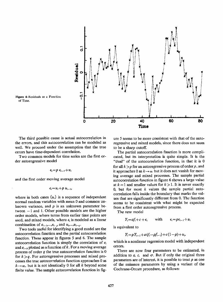
IOA:

SFigure 4-Residuals as a Functionof Time.

0

:if

IC

i t

-it

.,, * .

X , x~~~~~k

X x A . K.1

' X .. #,

I I ffi~~. ..

20 40Time

I

I

x Sb

If

:X

%V

...

I I I

60 80

The third possible cause is actual autocorrelation inthe errors, and this autocorrelation can be modeled aswell. We proceed under the assumption that the trueerrors have time-dependent correlation.

Two common models for time series are the first or-der autoregressive model

Ci=P Ei-1 +U;

and the first order moving average model

EijUj+p Up-1,

where in both cases luid is a sequence of independentnormal random variables with mean 0 and common un-known variance, and p is an unknown parameter be-tween - I and 1. Other possible models are the higherorder models, where terms from earlier time points areused, and mixed models, where ei is modeled as a linearcombination of ei-l fjp and Ui,...,Uiq_.

Two tools useful for identifying a good model are theautocorrelation function and the partial autocorrelationfunction. These appear in figures 5 and 6. The sampleautocorrelation function is simply the correlation of e;and ei-k plotted as a function of k. For a moving averageprocess of order q the true autocorrelation function is 0for k > q For autoregressive processes and mixed pro-cesses the true autocorrelation function approaches 0 ask ¢c, but it is not identically 0 for all k beyond somefinite value. The sample autocorrelation function in fig-

ure 5 seems to be more consistent with that of the auto-regressive and mixed models, since there does not seemto be a sharp cutoff.

The partial autocorrelation function is more compli-cated, but its interpretation is quite simple. It is the"dual" of the autocorrelation function, in that it is 0for all k >p for an autoregressive process of orderp, andit approaches 0 as k-co but it does not vanish for mov-ing average and mixed processes. The sample partialautocorrelation function in figure 6 shows a large valueat k = 1 and smaller values for k > 1. It is never exactly0, but for most k values the sample partial auto-correlation falls inside the boundary that marks the val-ues that are significantly different from 0. The functionseems to be consistent with what might be expectedfrom a first order autoregressive process.

The new model

Y 1=afi+c +Ei with Ej=pEiq_+Uj

is equivalent to

Yj=pYj_, +a(fj-pfiD)+c(l-p)+ui,

which is a nonlinear regression model with independenterrors.

There are now four parameters to be estimated, inaddition to a, c, and o-. But if only the original threeparameters are of interest, it is possible to treat p as oneof the nuisance parameters by using a variant of theCochrane-Orcutt procedure, as follows:

427

i

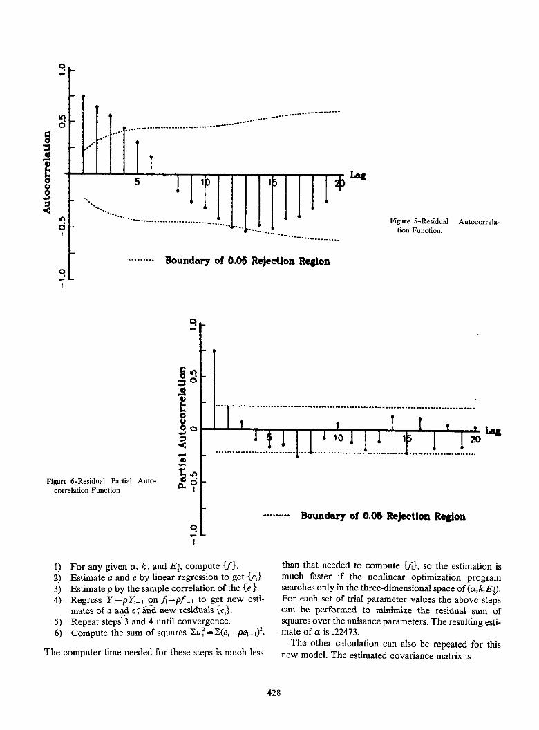
ooaq - hinI~V -- , ,_

l .Sin

C;-I

Figure 6-Residual Partial Auto-correlation Function.

.. ......... ............ _.…

LOS

Figure S-Residual Autocorrela-tion Function.

Boundary of 0.05 Rejeetion Region

e oS

c

:, o"C

0Z

t In

q

1) For any given a, kz, and E., compute ~ff1.2) Estimate a and c by linear regression to get {eJ}.3) Estimate p by the sample correlation of the {e,}.4) Regress Y1-pY,-, on fj-pt-, to get new esti-

mates of a and c, ;nd new residuals {e,.5) Repeat steps 3 and 4 until convergence.6) Compute the sum of squares Xu'=Y(ei-pei_,)-

The computer time needed for these steps is much less

.I .. . 1 _1 .I .-.I - - t 1.1 ' I t 1 2 0 . - . o.. d.. y.. .... .. . .. .. . ........ . ........ .

--------. Boundary of 0.06 Rejection Region

than that needed to compute {f1, so the estimation ismuch faster if the nonlinear optimization programsearches only in the three-dimensional space of (a,kE#j).For each set of trial parameter values the above stepscan be performed to minimize the residual sum ofsquares over the nuisance parameters. The resulting esti-mate of a is .22473.

The other calculation can also be repeated for thisnew model. The estimated covariance matrix is

428

I

terval that is about twice as long as the one in the inde-pendence model, but still only a third as long as theinterval obtained by O'Dea's procedure.

This is roughly four times the previous covariance ma-trix, so the length of the new confidence interval isabout twice that of the previous confidence interval.The new interval is [.22336, .22600].

The four intervals around a are compared in figure 7.The procedure used in O'Dea's original paper producesan interval obtained from a three dimensional con-fidence ellipsoid with a very large confidence level,and it is quite long. The interval is shortened by using a95% confidence ellipsoid, but it still does not have a95% coverage probability. The 95% confidence inter-val is still shorter. Taking into account the apparentautoregressive error structure leads to a confidence in-

Figure 7-Confidence Intervals forAlpha.

Thanks to Herman Chernoff for numerous discus-sions. Thanks also to IBM for providing graphics hard-ware and software.

References

[1] O'Dea, 1. J.; J. Osteryoung and R. A. Osteryoung, Square wavevoltammetry and other pulse techniques for the deter-mination of kinetic parameters. The reduction of zinc (II) atmercury electrodes, a Phys. Chem. 87, 3911-3918 (1983).

[2] Morrison, D. F. Multivariate Statistical Mehods, McGrawHill: New York (1976).

Based on the Factor 3

I I Based on the Factor 1.10

I- I-I Independence Model

I I Autoregressive Error Model

I0I.222 _ -, 00.222 0.224 0.226 0.228

429

4.8344-5.6256

.4766

-5.625637.5982

5-2.6193

.4766-2.6193

.6513] lo0-.

DISCUSSIONof the Lane-O'Dea-Osteryoung paper,Statistical Properties of a Procedurefor Analyzing Pulse Voltammetric Data

Janet Osteryoung

Department of ChemistryState University of New York at Buffalo

To supplement Lane's discussion of a statistical pro-cedure for analyzing pulse voltammetric data, I wouldlike to describe the experiment more fully in the contextof the scientific problem being addressed. In acontrolled-potential (voltammetric) experiment the cur-rent response generally depends on both potential andtime. Since the current is the rate of charge transfer, theresults of such experiments can be analyzed to yield thevalues of parameters that characterize the charge trans-fer process. The current for many charge transfer mech-anisms can be calculated, although often the results (acurrent-potential curve, or voltammogram) can be ob-tained only numerically. The calculated voltammogrammust be inverted to yield the values of the charge trans-fer parameters. It was the objective of O'Dea, et al. [Il'to devise a procedure for this inversion that would notdepend on either the charge-transfer mechanism or thechoice of voltammetric experiment. However the spe-cific problem addressed was that of determining thecharge transfer parameters for the reduction of Zn(II) atmercury electrodes in aqueous solutions of NaNO3 .

It was assumed at the outset that the mechanism ofcharge transfer was described by the Butler-Volmerequation

i(t) =nFAk e r[Do"'CO(O ,t)-,EDR112CR(O, t)]

where i(t) is the current at time t, n the number ofelectrons per zinc ion reduced, F the value of the Far-aday, A the electrode area, DO and DR the diffusioncoefficients of the oxidized (0) and reduced (R) forms ofzinc. CO (O,t) and CR (Oat) are the corresponding con-centrations at the electrode surface at time t,

c =exp[(nF/R T)(E(t)-Ell2)]

where R is the gas constant, T the absolute temperature,E(t) is the imposed potential, which is a function of time,and k, a, and E,,2 are the kinetic parameters as given by

Number in bracket is literature reference.

Lane. A mathematical model which describes exactlythe current-potential relation is developed by formu-lating the diffusion problem with the Butler-Volmer re-lation as a boundary condition and expressing the sur-face concentrations in terms of convolution integrals ofcurrents to yield an integral equation for the currentwhich can be solved numerically.

The typical procedure used in electrochemical kineticstudies is to measure Eml1 independently and to use itsvalue as a known quantity in analysis of the voltam-mogram. Furthermore, usually DO, DR, A, and n aredetermined in order to compare calculated and experi-mental currents directly. These additional pieces of in-formation are not necessary, however, and may intro-duce systematic error into the values of the derivedkinetic parameters. Because of the exponential form ofthe current-potential relation, minor errors in the valueof Ell2 distort the shape of the response and thereforecause errors in the derived value of a. These errors caneven suggest a potential-dependence of a which is anartifact. In a differential experiment such as square wavevoltammetry the response is generally peak-shaped, andthe height of the peak reflects the values of k and a.Errors of normalization (e.g., measurement of A) there-fore also introduce error into the values of the derivedparameters.

From the discussion of Lane et al., it is clear that thenormalization factor, a, is an unnecessary "nuisance"parameter, and thus it is foolish to confound the resultsof kinetic measurements by employing a method of dataanalysis which requires that a be known. The questionof E£12 is more subtle, for experimental and chemicalfactors must be considered. In principle, knowing thetrue value of Ell, simplifies the problem. Potential dif-ferences can be measured accurately, but it is difficult tomaintain a laboratory reference potential at a knownvalue over time. The data of [1] and the data employedby Lane et al. display confidence intervals for E£12 at the95% level of <0.001 V. Working laboratory standardsare not maintained with that precision. Chemical factors

430

must also be considered. The value of Eml1 is measuredusing either a voltammetric experiment with a muchlonger time scale or an equilibrium experiment. In thelatter case the diffusion coefficients must also be knownto yield Em11. In either case the change in time scaleintroduces the possibility of a change in mechanism,which produces a value of Ell2 inappropriate for theconditions of the kinetic experiment. Therefore Em11should be treated as an unknown parameter of the ex-periment together with k and a.

A further objective of this work was to obtain con-fidence intervals for the expectation values of the kineticparameters. Typically in experiments of this type uncer-tainty is estimated by estimating the coefficient of vari-ation of the current response and assigning that coeffi-cient of variation to the derived parameters, becausemore realistic procedures have not been available. Theprocedure presented by O'Dea et al. [1] has the merit ofcomputational simplicity and thus provides a well-defined quantity that can be used by the experimenter asa working figure of merit during the course of experi-ments. The procedure of Lane et al., which providesconventional confidence intervals with known con-fidence bound, relies on quadratic approximation of themodel, which should be adequate for well-behaved re-sponse surfaces.

Recent advances in theory and in computational ca-pabilities raise the possibility of fully quantitative the-oretical descriptions of at least some classes of electro-chemical reactions. Theoretical developments can beguided and tested using accurate data that have beenanalyzed using appropriate statistical techniques.

The work described in this report was supported inpart by the National Science Foundation under grantnumber CHE-8305748 and by the Office of NavalResearch.

References

[I] O'Dea, John J.; Janet Osteryoung, and R. A. Osteryoung, J.Phys. Chem. 1983, 81, 3911-3918.

431

Journal of Research of the National Bureau of StandardsVolume 90, Number 6, November-December 1985

Fitting First Order Kinetic ModelsQuickly and Easily

Douglas M. BatesUniversity of Wisconsin-Madison, Madison, WI 53705

and

Donald G. WattsQueen's University at Kingston, ON, Canada

Accepted: June 24, 1985

Kinetic models described by systems of linear differential equations can be fitted to data quickly and easily bytaking advantage of the special properties of such systems. The estimation situation can be greatly improvedwhen multiresponse data are available, since one can then automatically determine starting values and betterdiscriminate between rival models.

Key words: compartment model; deteniinant criterion; multiresponse estimation.

1. Introduction

In this article we summarize the work of a series ofpapers [1-3]' in which we deal with fitting first orderkinetic models to uniresponse and multiresponse data.

About the Authors, Paper: Douglas M. Bates is withthe Department of Statistics at the University of Wis-consin. Donald G. Watts is a member of the Departmentof Mathematics and Statistics, Queen's University atKingston. The work reported on was supported by theNational Science Foundation in the United States andthe Natural Sciences and Engineering Research Councilof Canada.

We consider systems in which the expected responsesat K points in the system, (t)=(7 11 (t), 72 (t), --- . (t))are described by the system of linear differential equa-tions

(1.])

where A is a K XK system transfer matrix depending onrate constants 0, 0 , ... , and ¢(t) is a vector input functionto the system. We assume further that there are K initialconditions V90=(O1o 0, ..n,.-, Ij77)0, some possibly un-known, and that r=t -Oo, where 0o is a (possibly un-known) time delay. All the unknown parameters aregathered into a P x I parameter vector 0.

433

l Numbers in brackets indicate literature references.

avla I =*O�A 27(0+40

Example: Oil Shale.!Asazrxarzpleaf a cherndcahwsstenm~desoribcd by s ,et

of linear differenrial equations, we cite; the pyrolysis ofoil shale in which the model, fitted by Ziegel andGornian [4] has the system diagram

6 6,

/ 61 °20*-l2-*-- II'1 1 3

0 3

In this system, 1 denotes kerogen, oo, bitumen, and )7Aoil. The model implies that kerogen decomposes to bitu-men with rate consisxt 0,, -and to oil with rate constant0,, and bitumen produces oil with rate constant 02, andunmeasured by-products with rate constant 03.

The integral of the vector function is evaluated com-gonentwise. CornpLtautual methods for .evaluadng theconvolution inregral are given in Moler and Vat. Loan[8], when A is diagonalizable, and in Bavely and Stewart[93, when A is nondiagonalizable.

22 Derivatives of the Expectation Function

To use a Gauss-Newton procedure to estimate theparameters we need derivatives with respect to the pa-rameters. As shown by Jennrich and Bright [6], a greatadvantage to compartment models is that the deriva-tives can be evaluated in she same fashion as the modelfunction itself. Instead of differentiating NQ) directly asin Jennrich and Bright, however, we differentiate eq(1.1) and solve the resulting linear system of differentialequations. This idea was discussed in another context inSmith [10! and was used by Kalhfleisch el at. [I l].

To simplify notation, we use a subscript p to denotedifferentiation with respect to the parameter Qp so

2. Expectation Functions andWith' Respect to the Parameters for

Kie tic Systems

DerivativesFirst Order

apt(t)

for p = 1, 2, ... P. The derivative of (1,1) with respect to0, is then

Several methods are used to estimate the parametersin first order kinetic models. The most obvious methodis to solve the system of differential equations corre-sponding to the particular comnpartment model and usethe resulting expectation function in a standard non-

linear estimation program. A second approach is to fit agenerai sum of axpnaetials rmodei by "peeling" [51, AThiru approach IS to use a sian&tArd nonlinear esimaDnprogram, using numerical integration to solve the equa-tions. A superior approach, proposed by Jennrich andBright 16]. is to obtain the general solution to the systemof equations by calculating values for the model func-tion Eiq) and its derivatives directly, given values of Band t and i(t).

2.1 The General Solution

The solution to a lineac systenm of differential equa-tions can be expressed in terms of convolutions using thematrix exponential [7]. The solution is

lQ)=e 'io~e"'*tft)

k (0 =-4 vp W +AP tt) + (P t)

for which the solution is

,q ,)= e' %9, (O) + e *IfAn(t) + tP (eN) (2.3)

' =e t t, - (t,) r + e ̀ *A PC.4S+e A AIe ,t f .

Dead time, 0,, can be incorporated by modifying ( 1. 1) to

i(,r) =A ti(r)+t,Q(0)=Vo

wherev-Go 2>Oo

r 0 t6O0 .

If 8o is known, we simply replace (by r in eqs 1.1, 2.1,and 2.3, but if Co is unknown and depends on a parame-ter, the expression for the derivatives is extended to

(Z. )

where the '*' denotes convolution,

e t~tL)f= J eA(-JNt(g de.

434

It is easy to evaluate A,,i, (0)=aio/a80, and r, sincethey are constants and, in fact, usually two of the threeare zero. Also, for any t <00, r, is zero for allp = 1, ... , P. Note that the method can be extended tohigher order derivatives.

Specifying the Model

A simple unambiguous computer notation can be usedto specify first order kinetic models in a parameter tableconsisting of three columns, the first column giving theparameter number. For a rate constant, the second col-umn entry gives its source and the third column entry itssink, a sink with compartment number 0 denoting elimi-nation. For initial conditions, 110, the second columnentry is the number of the component in 170 and the thirdcolumn entry is -1. For a step input, t, the secondcolumn entry is the number of the component in z andthe third column entry is -2. Dead time is coded as 0 incolumn 2 and 0 in column 3.

Example: Oil Shale.2

The oil shale parameter table is presented in annotatedform. It is to be noted that a single parameter may repre-sent more than one rate constant.

To determine the minimum of IZ'Z 1 it is advan-tageous to calculate the gradient and Hessian and ex-ploit Gauss-Newton optimization techniques. Efficientnumerical procedures for computing the gradient andapproximate Hessian are given in [2], and an algorithmwhich performs the calculations in [1].

Alternative expressions for the components of thegradient y and the Hessian r are

y,=81 VI/aO,=2I VItr[V-'Z'Z],p = 1,2,...,P I (3.2)

and

r'mq=a21 VI/opaOq= (3.3)

='peq+ 2 I VI tr[V-lZ'Z 0 V-Z'Zp]+21 Vltr[V-'Z'ZqV-'Z;Z]

+21 Vltr[V-'ZZq]+21 Vltr[V-'Z'Z,,p,q=1,2, .,P.

The second derivative terms Z,, in eq (3.3) are ignoredto produce an approximate Hessian.

Table 1. Oil shale parameters.

Parameter Column Columnnumber (type) 2 3

l (rate constant) I (source) 2 (sink)2 (rate constant) 2 (source) 3 (sink)3 (rate constant) 2 (source) 0 (elimination)4 (rate constant) I (source) 3 (sink)s (dead time) 0 0

3. Multiresponse Estimation

In the multiresponse situation when the errors haveunknown variances and covariances but are assumed tobe temporally uncorrelated, the appropriate criterionderived via a likelihood or Bayesian approach is to min-imize the M XM determinant [12].

l V(0) I = Z'Z I (3.1)

In eq-(3.1), Z= Y-H is the NXM matrix of residuals{Z0k}=Tkk(tl).-flk(t.)}, k = 1, ,2, ... , M, n = 1, 2,N. The expected responses 17 are assumed to depend on Pparameters 0: except where explicitly required, we sup-press the dependence on 0. For first order kinetic sys-tems with all responses measured, M =K.

4. Practical Aspects

Linear Constraints

Sometimes the data matrix Y involves dependenciesas a result of imputation of responses or mass-balancecalculations. If these dependencies also occur in the ex-pected responses, then important modifications to themultiresponse estimation procedure must be made so asto avoid convergence to spurious optima [13,14]. It istherefore necessary to examine the residual matrix Z(0)for singularities, which can be done by arranging therounding units in the columns of Y to be approximatelyequal and taking a singular value decomposition of Z[15]. As explained there, singular values on the order ofthe rounding unit indicate singularity and shouldprompt the analyst to search for constraints in the data.Such examinations should be done at the beginning ofthe analysis using the initial parameter values and at theend of the analysis using the converged values. To aidconvergence, logarithms of parameters are used duringestimation.

Linear constraints can be dealt with easily by com-bining the linear constraint vectors into a matrix, per-forming a QR decomposition of that matrix, and lettingthe rotation matrix W be the columns of Q which areorthogonal to the constraint vectors. We then simplyminimize I(ZW)'(ZW)I, where ZW=YW-HW.Clearly, the gradient and Hessian of this determinant

435

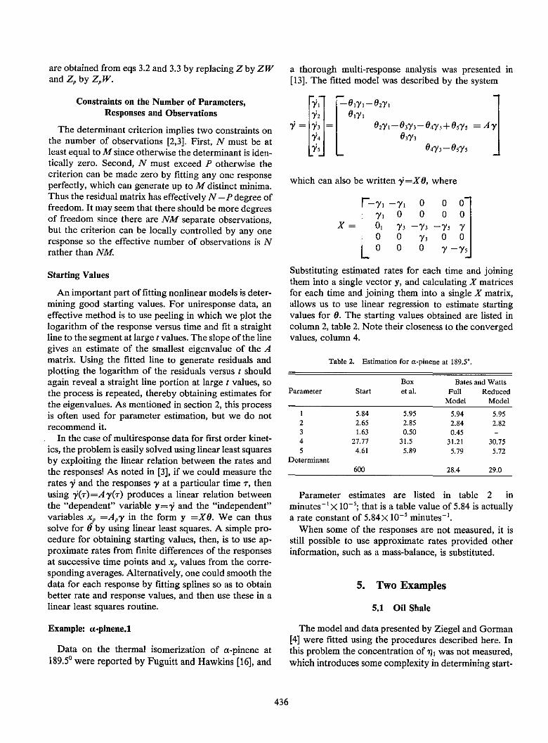
are obtained from eqs 3.2 and 3.3 by replacing Z by ZWand Z, by Z, W.

Constraints on the Number of Parameters,Responses and Observations

The determinant criterion implies two constraints onthe number of observations [2,3]. First, N must be atleast equal to M since otherwise the determinant is iden-tically zero. Second, N must exceed P otherwise thecriterion can be made zero by fitting any one responseperfectly, which can generate up to M distinct minima.Thus the residual matrix has effectively N-P degree offreedom. It may seem that there should be more degreesof freedom since there are NM separate observations,but the criterion can be locally controlled by any oneresponse so the effective number of observations is Nrather than NM.

Starting Values

An important part of fitting nonlinear models is deter-mining good starting values. For uniresponse data, aneffective method is to use peeling in which we plot thelogarithm of the response versus time and fit a straightline to the segment at large t values. The slope of the linegives an estimate of the smallest eigenvalue of the Amatrix. Using the fitted line to generate residuals andplotting the logarithm of the residuals versus t shouldagain reveal a straight line portion at large t values, sothe process is repeated, thereby obtaining estimates forthe eigenvalues. As mentioned in section 2, this processis often used for parameter estimation, but we do notrecommend it.

In the case of multiresponse data for first order kinet-ics, the problem is easily solved using linear least squaresby exploiting the linear relation between the rates andthe responses! As noted in [3], if we could measure therates 9 and the responses y at a particular time r, thenusing 9(7-)=Ay(T) produces a linear relation betweenthe "dependent" variable y=y and the "independent"variables xP =Apy in the form y =XO. We can thussolve for 6 by using linear least squares. A simple pro-cedure for obtaining starting values, then, is to use ap-proximate rates from finite differences of the responsesat successive time points and xp values from the corre-sponding averages. Alternatively, one could smooth thedata for each response by fitting splines so as to obtainbetter rate and response values, and then use these in alinear least squares routine.

a thorough multi-response analysis was presented in[13]. The fitted model was described by the system

'2 01yi

Ili5 = 3 =02/L°IY34O27V5

I-0373-04Y3 + 05Y=A M03Y3

04Y3 -05^)Y5

which can also be written y=XO, where

X= 01

0

L0

-7i0

7 300

00

-Y3

Y30

0 0 j0 0

-757KY-'Y

Substituting estimated rates for each time and joiningthem into a single vector y, and calculating X matricesfor each time and joining them into a single X matrix,allows us to use linear regression to estimate startingvalues for 0. The starting values obtained are listed incolumn 2, table 2. Note their closeness to the convergedvalues, column 4.

Table 2. Estimation for a-pinene at 189.5'.

Box Bates and wattsParameter Start et al. Full Reduced

Model Model

X 5.84 5.95 5.94 5.952 2.65 2.85 2.84 2.823 1.63 0.50 0.45 -4 27.77 31.5 31.21 30.755 4.61 5.89 5.79 5.72

Determinant600 28.4 29.0

Parameter estimates are listed in table 2 inminutes-'X 10-5 ; that is a table value of 5.84 is actuallya rate constant of 5.84X 10-' minutes-'.

When some of the responses are not measured, it isstill possible to use approximate rates provided otherinformation, such as a mass-balance, is substituted.

5. Two Examples

5.1 Oil Shale

Example: a-pinene.1

Data on the thermal isomerization of a-pinene at189.5' were reported by Fuguitt and Hawkins [16], and

The model and data presented by Ziegel and Gorman[4] were fitted using the procedures described here. Inthis problem the concentration of 7ll was not measured,which introduces some complexity in determining start-

436

ing values. Second, the elimination compartment, corre-sponding to coal and gas, was not measured. Third,there was a time delay caused by the shale having toreach the reaction temperature. The observed responsesare Y2 and y, , measured in percent of the initial kerogen711, so K=3, M=2, with N=14.

To determine starting values in this case, we plottedthe data and obtained a rough estimate of Oo=6 min.Estimating the initial slopes of i72 and 71 from the graphgave values of 0.029 min-' for 0, and 0.013 min' for 04 .This delay estimate and the rate constants were used toobtain starting estimates of 02 and 03 as shown in column2, table 3, following the procedure of section 4. The finalresults, together with those of Ziegel and Gorman, areshown in columns 3 and 4 of table 3.

Table 3. Parameter estimates for oil shale data.

Parameter Start Bates-Watts Ziegel-Gorman

1 0.029 0.0172 0.0173 (k,)2 0.012 0,0090 0.0092 (k2 f2)3 0.028 0.0205 0.0201 (k,(t-f,))4 0.013 0.0104 0.0104 (k3)Oo 6.0 7.8 7.7

Determinant67980 429

5.2 a-pinene

In their analysis of the a-pinene data, Box et al. [13]noted that response 4 was imputed usingy4=0.03(l00-y,), and that the data set was subject to amass-balance constraint, Y +Y2+Y3+Y4+Y5=100. Toavoid convergence to spurious optimal parameter val-ues, they recommended that these data dependencies betaken into account by using observation vectors consis-ting of linear combinations of y, , y, y,, y4 and ys whichare orthogonal to the space defined by the vectors(0.03, 0, 0, 1, 0)' and (1, 1, 1, 1, 1)'. We thereforetreaty 4 as an unmeasured component for estimation pur-poses, and use linear combinations of the responseswhich are orthogonal to the vectors a =(0, 0, 0, 1, 0)and a,=(l, 1, 1, 1, 1). The rotation matrix M and themodified responses can therefore be determined by per-forming a QR decomposition on the matrix (a,, a,) andusing the last 3 columns of Q coupled with all the re-sponses. In this case, K=5, M=3, with N=8.

Approximate 95% confidence limits for InO3 werevery wide, suggesting that 03 was badly estimated andcould be zero. We therefore fitted a reduced modelin which there was no path from ,33 to 714, see column 5.The change in the determinant is 0.6 on I degree offreedom, which, when compared with the scaling factors =28.4/3=9.46 on 3 degrees of freedom, is clearly

small, verifying that the reduced model is adequate forthis data set.

To further substantiate the adequacy of the reducedmodel, we fitted both models to a second set of datataken 204.50 [16]. The results of this fitting procedureare presented in table 4. The reduced model appears tobe adequate for both data sets.

Table 4. Estimation for a-pinene at 204.5'.

Full ReducedParameter Start Model Model

1 23.0 22.6 22.62 13.2 12.6 12.63 8.3 0.02 -4 76.9 72.8 72.85 16.0 15.6 15.6

Determinant116 0.55 0.55

6. Conclusions

Several advantages of the direct multiresponse esti-mation approach for systems of differential equationsare apparent. First, the model can be specified directlyfrom the network diagram. Second, there is no need toobtain the analytic solution to the differential equationsdescribing the reactions. Third, there is no need to codethe model functions in a nonlinear estimation routine.Fourth, the bothersome and error-prone step of obtain-ing and coding derivatives of the expected responseswith respect to the parameters is eliminated. Fifth, ex-cellent starting values can be determined automatically.

References

[I] Bates, D. M., and D. G. Watts, A multi-response Gauss-Newtonalgorithm, Commun, Statist.-Simul. Comput. B(13),705-715 (1984).

[2] Bates, D. M., and D. G. Watts, A generalized Gauss-Newtonprocedure for multi-response parameter estimation, SIAMJournal on Scientific and Statistical Computing, to appear.

[3] Bates, D. M., and D. G. Watts, Multiresponse estimation withspecial application to systems of linear differential equations,Technometrics 27, 190-201 (1985).

[4] Ziegel, E. R., and J. W. Gorman, Kinetic modelling with multi-response data, Technometrics 22, 139-151 (1980).

[5] Anderson, D. H., Compartmental modeling and tracer kinetics,Springer-Verlag (1983).

[6] Jennrich, R. I., and P. R. Bright, Fitting systems of linear differ-ential equations using computer generated exact derivatives,Technometrics 18, 385-392 (1976).

[7] Noble, B., Applied linear algebra, Prentice Hall (1969).[8] Moler, C., and C. Van Loan, Nineteen dubious ways to compute

the exponential of a matrix, SIAM Review 20 (1978).

437

[9] Bavely, C A, and G. W. Scewart, An agorilhmr frcornputir.g [131 Bc^ G. .E. P,; W. G. Bunter, J. F. MacGregzr, and J Erjavcz,reducing subspaces by block diagonalizalion, SIAM Journal Some problems associated with the analysis of multiresponseof Numerical Analysis 16, 359-367 (1979). data, Technometrics 15, 33-51 (1973),

[lo) SmilhW. R., Parameter es14mation i nonlinear modelS of bo- [14] McLean, D. D.; D J. Pritchard, D. W. Bacon, and J. Downie,logical systems, Fisheries and Marine Services Technical Sirgvlarities in multiresponse modelling, Technometrics 21,Report 889, Fisheries and Environment Canada (1979). 291-298 (1979).

[l11 Kalbfleiscl,3J.D.;J.LF.LawlessandW M.Vottmier,Estimation 115] Dongarra, J. J.; J. R. Bunch, C. B. Moler, and G. W. Stewartin Markov models from aggregate data, Diornetrics 39, Linpack User's Guide, Chap. 11, Philadelphia: S.IA.M.9fl7.-g9 (1%3), (1979).

[12] Box, G.E. P.. and N. R. Draper, The Bayesian estimation of (16] Fugutut,R E.,andI.E.Hawkins Rateofthermalisomerizationcommon paramelers from several responses, Biomemrika 52, of a pineue in the liquid phase, J. Amer. Chem. Soc. 69,355-365 (1965), 319-312 (1947).

DISCUSSIONof the Bates-Watts paper,Multiresponse Estimation With SpecialApplications to First Order Kinetics.

Michael Frenklach

Department of Materials Science and EngineeringPennsylvania State University I

The authors presented an interesting approach to pa-rameter estimation for first order kinetic systems. Themethod is user oriented and particularly suited for com-puter implementation as a "canned" program. Indeed,present chemical kinetic codes input reaction rnech-anism in a natural chemical language, that is, specifyingreactions (usually in unformatted READ routines) asthey are conventionally written on the paper. This infor-mation is automatically converted to a so-called reac-tion matrix and, based on it, to differential equationsdescribing the kinetics of reaction species. The reactionmatrix, which contains all the stoichiometry of the sys-tem, can conveniently provide the required input infor-

'Michael Frenklach's contribution to the subject stems from workperformed in the Departmnent of Chemical Engineering, LouisianaState University.

Another important feature, from the user's point ofview, is that the presented method is applicable to mul-tiresponse data. It should be realized that modern prob-lems of interest to chemical kinetics get tougher, as fotexample, formation of pollutants in hydrocarbon com-bustion. The experimental answer to the growing com-plexity of the systems is the employment of multiplediagnostics for simultaneous monitoring of various pro-cess variables. However, interpretation of the experi-mental results cannot be fully realized without reliableand convenient multiresponse methods.

The following are some of my thoughts on the needsin this area:

I) Oftea, kineticists exhibit a philosophical re-sistance to a multiparamneter approach to experi-mation for automatic coding of the method of Bates andWatts.

438

mentation. A classical way is to "isolate" a given reac-iton of interest; under such conditions the ratecoefficient parameters can be determined by a simplewell-established straight-line treatment. Determinationof more than one rate coefficient in a single set of experi-ments is considered "not clean experimentation." Inprincipal, however, the isolation is not possible: thereare always other reactions occurring simultaneouslywith the one of interest. The researchers usually engagein an elaborate line of reasoning to assume, sometimesunjustifiably, single-reaction conditions. These kinet-icists must realize that multiparameter analysis using rig-orous multiresponse techniques can provide more accu-rate and informative answers. Neglecting, for instance, achemical reaction with the rate contribution of, let ussay, 10%, can lead to a much larger than 10% distortionin the estimation of the main parameter. Statisticians, onthe other hand, should demonstrate the techniques theydevelop on examples of current interest and difficulty.

2) Although first order kinetic models constitute animportant class, higher order kinetics are of more gen-eral interest and there is a great need for development ofstatistical methods for these nonlinear systems.

3) Most estimation methods, including the onepresented by Bates and Watts, concentrate on deter-mining the solution which minimizes the objective func-tion and only approximate confidence limits. What is ofinterest to many applications is the joint confidence re-gion. It should be noted that in the problems of chemicalkinetics these regions are usually not ellipsoidal, forwhich second order approximation methods are suf-ficient, but crescent shaped.

4) While estimating parameters, it is most importantto check the model adequacy. This point was excellentlydemonstrated by Box and Draper (1965). These authorswarn that "the investigator should not resort immedi-ately to the joint analysis of responses. Rather heshould... consider the consistency of the informationfrom various responses." To my knowledge, however, aformal multivariate lack-of-fit test for a general non-linear case has not been developed.

5) A question on the number of degrees of freedom

was brought up by Bates and Watts. Using fastdigital sampling electronics, the number of observationsper response can be very large (in our laboratory thisnumber was approximately 1000). Does this number de-termine the degrees of freedom? If so, then one caneasily increase this number by orders of magnitude byusing faster electronics. This point should be clarified.

Finally, I would like to point out that in an attempt toresolve some of the issues brought up above, a methodfor multiresponse parameter estimation applicable to adynamic model of general order was developed in ourlaboratory (Miller and Frenklach, 1983; Frenklach,1984; Frenklach and Miller, 1985). The method is basedon approximating the solution of the differential equa-tions describing the kinetics of reactive system instead ofthe equations themselves. The approximation is devel-oped following the methods of empirical model building(Box et al. 1978) and the concept of computer experi-ment of Box and Coutie (1956). Once the approxi-mations to all responses are obtained, the parameter esti-mation, determination of joint confidence region, andlack-of-fit test are easily performed following the ap-proach of Box and Draper (1965).

References

[1] Box, G. E. P., and G. A. Coutie, Application of digital computersin the exploration of functional relationship, Proc. I.E.103B (Suppl. No. 1) 100-107 (1956).

[2] Box, G. E. P., and N. R. Draper, The Bayesian estimation ofcommon parameters from several responses, Biometrika 52,355-365 (1965).

[3] Box, G. E. P.; W. C. Hunter and J. S. Hunter, Statistics forExperimenters. An Introduction to Design, Data Analysis,and Model Building, Wiley: New York (1978).

[4] Frenklach, M., Modeling, Combustion Chemistry (Edited by W.C. Gardiner, Jr.), Chap. 7, Springer-Verlag: New York(1984).

[5] Frenklach, M., and D. L. Miller, Statistically rigorous parameterestimation in dynamic modeling using approximate empiricalmodels, AICHE J. 31, 498-500 (1985).

(6] Miller, D., and M. Frenklach, Sensitivity analysis and parameterestimation in dynamic modeling of chemical kinetics, Int. J.Chem. Kinet. 15, 677-696 (1983).

439

Journal of Research of the National Bureau of StandardsVolume 90, Number 6, November-December 1985

The Use of Kalman Filteringand Correlation Techniques

in Analytical Calibration Procedures

H. C. Smit

University of Amsterdam, Nieuwe Achtergracht 166, 1018 WV Amsterdam, The Netherlands

Accepted: June 24, 1985

Different chemometric methods to improve calibrations are described. A Kalman filter is applied for

processing and predicting slowly varying parameters of a linear calibration graph. The results are used for theevaluation of unknown samples, and for deciding whether to calibrate again or to analyze the next unknownsample. Another approach of the calibration problem, particularly in chromatography, is the use of cor-relation techniques. The noise reduction property of correlation chromatography is used to extend thecalibration graph to very low concentrations. Furthermore, an experimental technique to determine a cali-bration curve and the unknown sample simultaneously under exactly the same conditions is described.

Key words: calibration; chromatography; correlation techniques; Kalman filter.

1. Introduction

The computer has added a new dimension to anal-ytical chemistry. Chemometrics, the application ofmathematical and statistical techniques, is improving thequality of the analytical results concerning accuracy,precision, time, and costs, and has created new possi-bilities. An extended number of chemometric pro-cedures are now available and are being increasinglyapplied in practice.

However, the "off-line" application of chemometricprocedures, i.e., the processing of data or signals alreadyobtained with common analytical methods like titration,chromatography, spectroscopy, etc., is dominating. Thecomputer is generally used as an off-line calculationmachine. The incorporation of the computer into exist-ing analytical methods or the development of new meth-

About the Author, Paper: H. C. Smit is with theUniversity of Amsterdam's Laboratory for Anal-ytical Chemistry. The work he describes was sup-ported in part by the Netherlands Research Or-ganization ZWO.

ods based on the capabilities of the computer is not fardeveloped; the intelligent analyzer is still in its infancy.

In this paper, some examples of chemometric on-linecomputer applications in an analytical procedure andanalytical method are given. The calibration, which isvery important in analytical chemistry, is emphasized inboth examples-a generally applicable procedure usingan optimum recursive parameter estimation technique(vector Kalman filter), and a method developed for oneparticular analytical technique (chromatography).More details concerning the basic theory are given in

[l]'.

Calibration and Optimum Estimation

An analytical system is usually very complex and in-cludes chemical, optical, electrical, and mechanicalparts. All these parts are subject to several influences,like contamination, changes in temperature, humidity,etc., and, of course, aging. These influences result in adecrease of the quality of the analytical data. Two main

I Figures in brackets indicate literature references.

441

components can be distinguished: a stochastic com-ponent resulting in stationary random fluctuations, anda semi-random component caused by irreversible pro-cesses like the mentioned contamination, aging etc. Thissemi-random component has a non-stationary natureand a regular calibration is required to maintain thequality of the results respectively to reduce the influ-ence of the drift in the calibration parameters. Ignoreddrift seriously affects the accuracy in the analytical re-sults and various off-line drift correction procedureshave been proposed [2-6].

A Kalman filter enables on-line drift compensation,particularly suitable in the case of automated analyticalprocedures. An optimum recursive estimator like aKalman filter requires a model of both the system or thesignal process, including the system noise and the mea-surement (observation) noise. Using an appropriatemodel, the Kalman filter can predict (estimate) futurevalues of the changing parameters and the samples canbe evaluated using these predicted parameters. The esti-mation may also be used to determine when a re-calibration is required. The criterion is a given presetprecision of the results. The final goal is to analyzesamples with a predetermined minimum accuracy.

System Model

A state space model is used to describe the system.The linear discrete dynamic system

x(k)=F(k)x(k-l1)+w(k-l) (1)

whe

z(k)=h'(k)x(k)+ v(k)

:re

k :a time or a sequence nurnx(k) in Xl state vectorF(k) :n Xn transition matrixh'(k) :1I X n measurement vectorz(k) :measured signalw(k - 1):n X I system noise vectorv(k) :scalar measurement noise

(2)

her

is representative for many analytical systems (fig. 1).The model is linear because neither in the transitionmatrix F(k) nor in the measurement vector h'(k) param-eters x(k) are present. A commonly used calibrationgraph is

y =a *c +b

where

a: sensitivityb: intercept

(3)

c: concentrationy: measurement

Reformulation gives

y=(c,l)bUsing

(b) an( z)

h'= (c, 1) and z =y

and adding system noise and measurementin a dynamic calibration curve

(4)

(5)

noise results

(a (k)\( O= ja(k-l)\ fwi(k-l)\(b(k)I k0lIJkb(k- I)) +w2(k -1)]

z(k)=(c,l)( a(k) )+ v(k).

(6)

(7)

A common situation in practice is that the parametersof the calibration curve are slowly varying in time. Sto-chastic variations can be represented by the systemnoise, introduced in the model. However, in practiceoften a deterministic variation of the calibration parame-ter can be observed; particularly an extension of themodel with a linear drift increases the usability.

A single parameter (state) x, affected by a linear driftin the sequence k can be written as

x(k)=dk +e

where

d: (constant) drift parameter

e: x(0)

Evaluation of eq (8) leads to

x(k)=d(k-l)+d +e

=x(k-t1)+d.

(8)

(9)

The introduction of system noise and measurementnoise gives

(10){x(k)\ I x(k -1)) w,(k -1)d(k) I I) )d(kl I)dk 1w2(k-f))

z(k)=(1,0) ((k))+v k).

442

Figure 1-Linear dynamic system.

If both the sensitivity a and the intercept b are influ-enced by random drift, two extra parameters have to beintroduced in the original model. The final model is

a(k)b k)

a(k)/3(k)

10100101-0010000 1

a(k-I)ba(k-1)a(k-l),/3(k-l)

w, k-1)

+ w3 (k-1)w4 (k-1) (I 1)

mate the slope, the intercept, and the drift parameters ofthe calibration curve [7]

x(k/k - I)=F(k)i(k - I/k -1)

P(k/k - 1)=F(k)P(k - I/k - I)F'(k)+Q(k -1)

x(k/k)=i(k/k - l)+k(k){z(k)-h'(k)i(k/k- 1)

(13)

(14)

(15)

a(k)b (k)a(k) +v(k).:6(k)

The observability matrix is

C, C2 C3 C4

11 I1 10 c2 2c3 3c4

0 1 2 3 .

P(k/k)=P(k/k - l)-k(k)h'(k)P(k/k -1)

k(k)=P(k/k - I)h(k){h'(k)P(k/k - I)h(k)+

(16)

(17)

where:

(12)

The system is observable if there are at least twodifferent concentrations.

Q(k): system noiseR (k): measurement noisek(k): Kalman gain factor (correction factor)

Equation (18) gives the innovation, i.e., the differencebetween the experimental and the estimated mea-surement

Sample Evaluation and Recalibration

Assuming the transition matrix F(k) in eq (11) isknown exactly and the measurement vector h'(k) isknown from the calibration, and assuming the statisticalproperties of the system noise and measurement noiseare known ("white" noise with zero mean and normalprobability density function (pdf), the usual Kalman fil-ter algorithms, given in eqs (13-17), can be used to esti-

v(k)=z(k)-h'(k)i(k/k - 1) (18)

with

E{v(k)}=0

E{v(k)v'(l}={h'(k)P(k/k-l )h(k)+R (k)}S(k,l)- (19)

The variance of the predicted measurement is also

443

v(k)+ z (k )

W(K-I)

z(k)=(c,1,0,0)

I-

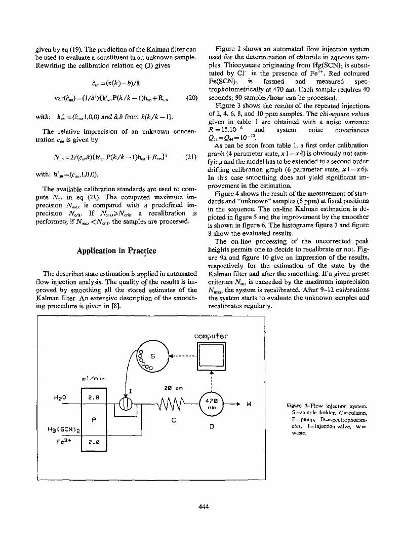
given by eq (19). The prediction of the Kalman filter canbe used to evaluate a constituent in an unknown sample.Rewriting the calibration relation eq (3) gives

2, = (z(k) -b)l

var(.,) = (l/a 2){h'. P(k /k - l)h,, + Ru, (20)

with: hi. =(&u,,1,0,) and &,b from k(k/k-1).

The relative imprecision of an unknown concen-tration ca. is given by

Nun=2/~cun&){h%,n P(k/k - l)h~s+R '}1 (21)

with: hu=(cl,, 1,0,0).

The available calibration standards are used to com-pute Nu. in eq (21). The computed maximum im-precision NmV, is compared with a predefmned im-precision NH,. If N,,,>NC6 ,, a recalibration isperformed; if New < N,, the samples are processed.

Application in Practice

The described state estimation is applied in automatedflow injection analysis. The quality of the results is im-proved by smoothing all the stored estimates of theKalman filter. An extensive description of the smooth-ing procedure is given in [8].

Figure 2 shows an automated flow injection systemused for the determination of chloride in aqueous sam-ples. Thiocyanate originating from Hg(SCN) 2 is substi-tuted by Cl- in the presence of Fe3". Red colouredFe(SCN)3 is formed and measured spec-trophotometrically at 470 nm. Each sample requires 40seconds; 90 samples/hour can be processed.

Figure 3 shows the results of the repeated injectionsof 2, 4, 6, 8, and 10 ppm samples. The chi-square valuesgiven in table I are obtained with a noise varianceR =15.lo-6 and system noise covariancesQ,3 = Q4= 10- 10

As can be seen from table 1, a first order calibrationgraph (4 parameter state, x I-x4) is obviously not satis-fying and the model has to be extended to a second orderdrifting calibration graph (6 parameter state, xl -x6).In this case smoothing does not yield significant im-provement in the estimation.

Figure 4 shows the result of the measurement of stan-dards and "unknown" samples (6 ppm) at fixed positionsin the sequence. The on-line Kalman estimation is de-picted in figure 5 and the improvement by the smootheris shown in figure 6. The histograms figure 7 and figure8 show the evaluated results.

The on-line processing of the uncorrected peakheights permits one to decide to recalibrate or not. Fig-ure 9a and figure 10 give an impression of the results,respectively for the estimation of the state by theKalman filter and after the smoothing. If a given presetcriterian Ncr,, is exceeded by the maximum imprecisioneNm.. the system is recalibrated. After 9-12 calibrationsthe system starts to evaluate the unknown samples andrecalibrates regularly.

computer

4? 0 N Figure 2-Flow injection system.S=sample holder, C=column,P = pump, D=spectrophotom-

D eter, l=injection valve, W=waste.

444

Figure 3-Repeated injections

Figure 4-Standards and unknown samples.

Table 1. Values ofx 2 for the flow injection peaks of figure 3.

Peak height Peak height Peak integral/300 Peak integral/300baseline corrected corrected

Kalman filter 618.8 662.7 134.9 797.2

(1st order)

Smoothed 578.7 620.1 122.0 744.2

(1st Order)

Kalman filter 69.8 67.5 61.0 395.4(2nd order)

Smoothed 62.0 59.3 53.8 354.4(2nd order)

Figure 5-On-line Kalman esti-mation.

01 -

I -

6.20 -

0.0a -

,le6-

-. 26 -

' ""1~~~~. :....,,,,,,,,,........ 1'11':::::::::::::::.

it" ..*.-.........- II ...... AdU,~~~~~~~~~~lp m

Is 36 54 72 90 -- > k

445

X3X2

XGXI8X3.10xi443xl

I

I

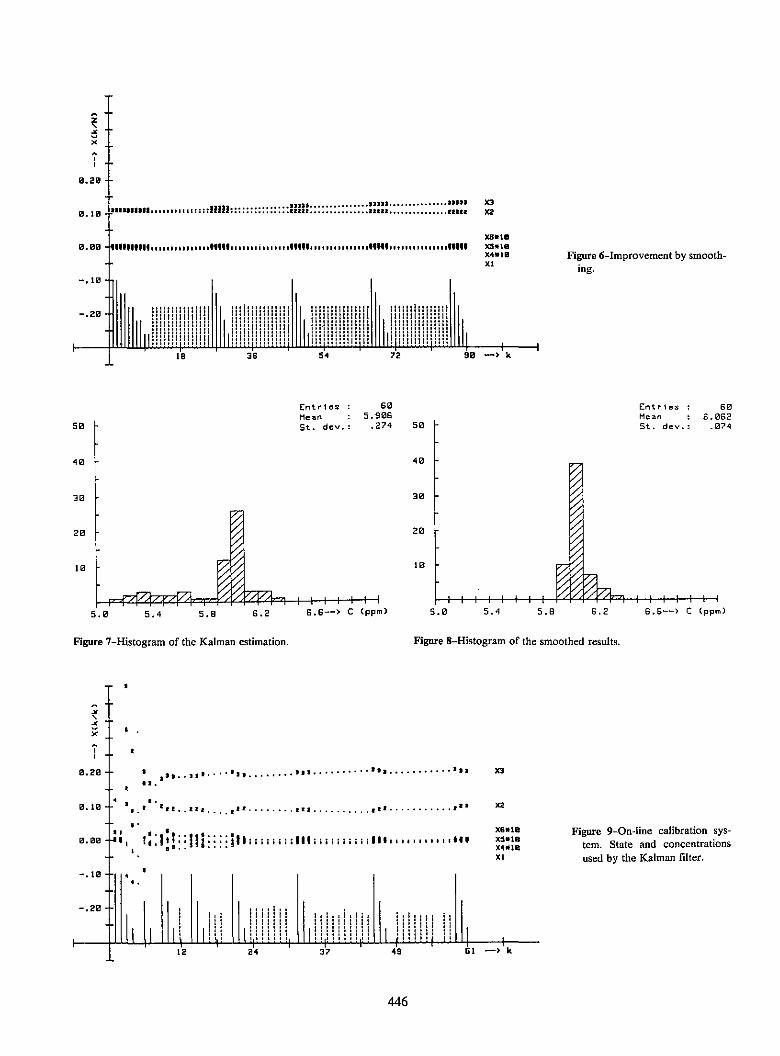
2

0.20

6. l

0.00 -fitiiiggguiFigure 6-Improvement by smooth-ing.

Entrles : 60Mean : 5.90bSt. dcv.: .274

5.0 5.4 5.H 6.2 6.6--> C (ppm)

Figure 7-Histogram of the Kalman estimation.

.

, ,-..-' '............ I". , .. m. '- I .1.

50

40

30

20 .

5.8r I I I I I r ..0 5.4 S.E

5<5<

5<5<5<5<5<

/5<6 II 6 C I I I m6.2 S.S--> C (pp.)

Figure 8-Histogram of the smoothed results.

....-....-... .

,.......... . .............a..............

M3

XZ

- i ? t5. 'I l ; ;;; IIIII ;II;;;I;IIII .. .. I I. . I. I IX6.10x"*.leX4l1ixi

Figure 9-On-line calibration sys-tem. State and concentrationsused by the Kalman filter.

49 63 -> k

446

-. 3

.20

........... ... , ,,11l::::.......li.......::::::: :::::: . .............. $1111............... X 2 11X4*le

xi

i i t I .. .. I II F i iiiii I E IIii

3b 54

Iii

it:I!!!

90 -> k72

40

30

20

1 0

Entries : 60M.ean : G.0l2St. dcv.: .074

8.20 -

0.36-

-. Ic

-. 20

I I I It ;12

11IIIII24

- lI I .

37

. I

. II

II1 iII.III

t:lm; ;:11::ii: itI I I I I I II I I I I I I I I. . � I

; . . ... ...... .. .. . ... .. ........... ...... .............

8 . .........ta .....r0.00 +ts I,I I I.Im I .... of ,f....... o f m.......... off ........... off

Figure 10-On-line calibration sys-tem. State and concentrationsused by the smoother.

Correlation Techniques

The introduction of correlation techniques permits acompletely different approach to the calibration prob-lem, particularly in chromatography. In correlationchromatography (CC) the usual impulse-shaped injec-tion is replaced by multiple random injections. An exam-ple of an application is given in [9]. The resulting ran-dom response of the chromatographic system iscross-correlated with the used input function. Thecross-correlation function of two signals, in this case theinput signal x(t) and the output signal y(t) of a linearprocess, is by definition:

However, the autocorrelation function of x (t) is definedas:

(26)

and eqs (25) and (26) can be combined to:

RxyQt2)= ){h(r)Rxx(t2-tnr)dr (7r>0) (27)

If x(t) is stationary, then:

(28)

and eq (27) becomes:(22)

(29)E[ ] denotes the expected value of the expression be-tween the brackets. The output signal y(t) of a linearsystem can be calculated as a convolution of the inputsignal x(t) and the impulse response h (t) of the system:

y(t)=x(t)*h(t)=ft h(r)x(t-r)d. (23)

Combining eq (22) and eq (23) gives:

R,(t 3te2)=E [x(t){ h (r)x(t 2 - T)dr] . (24)

In this case integration and averaging can be inter-changed, hence:

Rx,(tit 2)= f h (T)E[x (tl)x(t2-r)]dr (25)

Comparing eq (23) and eq (29) shows that the outputsignal y(t) of a linear system with an input signal equalto the autocorrelation function R.(t) of a signal x (t) issimilar to the cross-correlation function RX,(t) of theinput signal x(t) and the output signal y(t) resultingfrom x(t).

A white noise, that is, white with respect to the band-width of the system, has in impulse-shaped auto-correlation function and can be used as input functionx(t) to determine the impulse response, in which caseRy(t) =h (t).

On further consideration a chromatographic pro-cedure can be regarded as the determination of an im-pulse response; a chromatogram shows the response onthe impulse-shaped injection of the sample. The primeobjective of correlation chromatography is to determinethe chromatogram by stochastically injecting the sam-

447

z

0.20

0.

-. 10 -

-.20 -

X3

X2

X'4*1

xi

- I : 1 1 1 ' ;1 it 1 1 1 .:. .:%~ I .

I2 24

Li I. I

37

i!!!!!! .11it*i iS i I it

49 61 -> k

R. Q1,t2) = E [x QOIX Q2)]

R. (t1,t2-,r) =R(t2-r-t,)= R (t -- r)

RQ1,t2)=E[x(t1)y(t2)]

RQ1,t2)=R,(t)= f h(,r)R.(t-,r)dr

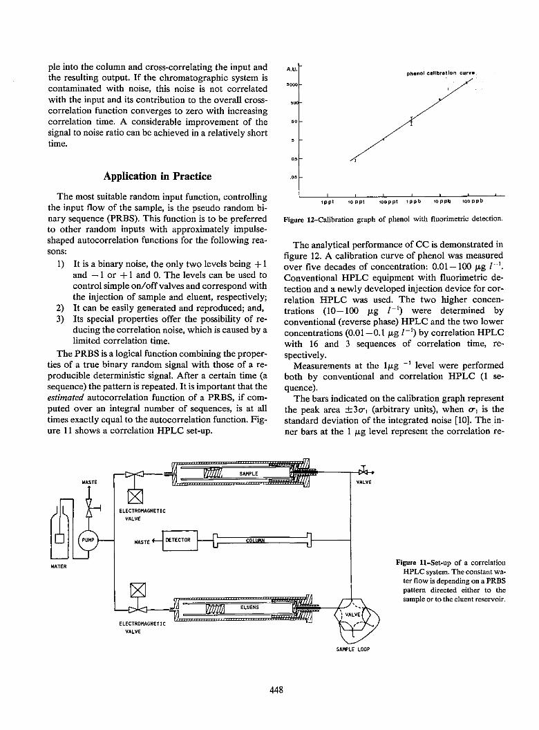
ple into the column and cross-correlating the input andthe resulting output. If the chromatographic system iscontaminated with noise, this noise is not correlatedwith the input and its contribution to the overall cross-correlation function converges to zero with increasingcorrelation time. A considerable improvement of thesignal to noise ratio can be achieved in a relatively shorttime.

AU.

5001-

50

0.

Application in Practice

The most suitable random input function, controllingthe input flow of the sample, is the pseudo random bi-nary sequence (PRBS). This function is to be preferredto other random inputs with approximately impulse-shaped autocorrelation functions for the following rea-sons:

1) It is a binary noise, the only two levels being + Iand - I or + 1 and 0. The levels can be used tocontrol simple on/off valves and correspond withthe injection of sample and eluent, respectively;

2) It can be easily generated and reproduced; and,3) Its special properties offer the possibility of re-

ducing the correlation noise, which is caused by alimited correlation time.

The PRBS is a logical function combining the proper-ties of a true binary random signal with those of a re-producible deterministic signal. After a certain time (asequence) the pattern is repeated. It is important that theestimated autocorrelation function of a PRBS, if com-puted over an integral number of sequences, is at alltimes exactly equal to the autocorrelation function. Fig-ure 11 shows a correlation HPLC set-up.

.05

phn calib aion cur.

ppt .0 Ppt '00ppt ppb .o ppb .o0 Ppb

Figure 12-Calibration graph of phenol with fluorimetric detection.

The analytical performance of CC is demonstrated infigure 12. A calibration curve of phenol was measuredover five decades of concentration: 0.01 -100 pg -'.Conventional HPLC equipment with fluorimetric de-tection and a newly developed injection device for cor-relation HPLC was used. The two higher concen-trations (10-100 gg /') were determined byconventional (reverse phase) HPLC and the two lowerconcentrations (0.01-0.1 jvg 1-;) by correlation HPLCwith 16 and 3 sequences of correlation time, re-spectively.

Measurements at the 1 ig -' level were performedboth by conventional and correlation HPLC (I se-quence).

The bars indicated on the calibration graph representthe peak area ± 3o-, (arbitrary units), when a-, is thestandard deviation of the integrated noise [10]. The in-ner bars at the 1 Mig level represent the correlation re-

Figure 1l-Set-up of a correlationHPLC system. The constant wa-ter flow is depending on a PRBSpattern directed either to thesample or to the eluent reservoir.

SAMPLE LOOP

448

suits and the outer bars the single injection results. Thedetection limit for the single injection experiments, de-fined as 3o-,, was about 0.5 Mtg 1'. The detection limitwith the 10 ng t1 concentration was estimated to be 3ng l' (3 ppt).

Simultaneous Correlation Chromatography

On further consideration, the question arises whetherit is possible to inject different samples simultaneously,each sample injection controlled by its own uniquePRBS. If these pseudo random sequences are mutuallyuncorrelated, then the correlogram (chromatogram) ofeach sample can be determined without any influence ofthe other samples, even if the components in the samplesare the same. The problem is to find uncorrelatedsequences.

A possible solution is the following. A binary pseudorandom noise sequence is generated by a digital shiftregister with a suitable modulo-2 feedback. Appropriatedigital multiplexing yields multiple uncorrelated pseudorandom outputs from a single n-bit shift register. Eachof the K output sequences is identical to the single shiftregister sequence; they are staggered by 24/K bits, sothey will remain uncorrelated for l/K(2 0 -1) outputbits. These output sequences can be used for the men-tioned simultaneous input patterns of a chro-matographic column.

Figure 13 shows the result of a simulation experiment.A separation of two components is simulated with fourdifferent samples which were "injected" simulta-neously. The "separation" is excellent.

The injection of n samples requires a correlation timeof n times the total elution time. Therefore, no time gaincan be expected. However, the method can be used fora number of interesting applications. For example, si-multaneous CC permits measurement and calibration at

PRES I

PROS 2

PROS 3

Figure 13-Simulated simultaneous chromatogram.

the same time under the same chromatographic condi-tions.

Figure 14 shows an experimental set-up of a simulta-neous chromatograph (HPLC) with four reservoirs(three samples and eluent) together with four valves,each controlled by a sequence uncorrelated with theothers. The flow stability is maintained by dividing aclock period in four parts. In each part either eluent orsample (respectively sample 1, 2, and 3) can be injected,depending on the status (0 or 1) of the sequence con-cerned.

The results of the analysis of three samples with naph-talene, anthracene, and 1,2 benzanthracene is shown infigure 15. The anthracene concentration in each sampleis the same; the concentration of the other componentsin the different samples differ by a factor of 2.

The experimental injection system is not yet perfect,and because of this, serves as a source of so-called cor-relation "noise." This noise is not really random, but is

oETECTOR

Figure 14-Experimental set-up of asimultaneous HPLC system.

449

TIME CS)

.50 1.00 1.50 E=0 2.50

CONC. 1. 2-ENZANThRACENE ('g/l)

Figure 15-Simultaneous chromatogram of three samples, each con-taining naphtalene, anthracene and 1,2 benzanthracene with differ-ent concentrations.

Figure 16-Calibration graph for benzanthracene, simultaneouslydetermined.

Figure 17-Calibration graph for benzanthracene, successively deter-mined.

composed of deterministic signals (ghost peaks). Thepeaks of benzanthracene are used to construct a cali-bration curve (fig. 16). Comparison of this curve withthe calibration curve determined in the usual way (fig.17) shows the performance of the method. The advan-tages are twofold: the random fluctuations are reducedby the multiple injection and averaging property, andboth the unknown sample and the calibration sample aremeasured simultaneously under exactly the same condi-tions.

The final conclusion is that on-line chemometric tech-niques, such as Kalman filtering and correlation pro-cedures, create promising new possibilities in analyticalchemistry. The given improvements of the calibrationprocedure are a typical example of the power of thesetechniques.

Major contributions to this paper were made by P. C. Thijssen, J. M. Laeven and C. Mars.

References

[I] Thijssen, P. C.; S. M. Wolfrum, G. Kateman, and H. C. Smit,Anal. Chim. Acta 256, 87 (1984).

[2] Nisbet, J. A., and E. Simpson, Clin. Chim. Acta 39, 367 (1972).(3] Nisbet, J. A., and J. A. Owen, Clin. Chim. Acta 92, 367 (1979).[4] Bennett, A.; D. Gartelman, J. J. Mason, and J. A. Owen, Clin.

Chim. Acta 29, 161 (1970).

[5] Svehla, G., and E. L. Dickson, Anal. Chim. Acta 136, 369(1982).

(6] Mclelland, A. S., and A. Fleck, Ann. Clin. Biochem. 15, 281(1978).

(7] Gelb, A., (Ed.), Applied Optimal Estimation, MIT Press, Cam-bridge, MA, USA (1974).

(8] Thijssen, P. C.; G. Kateman and H. C. Smit, Anal. Chim. Acta(submitted for publication, 1985).

[9] Smit, H. C.; T. T. Lub and W. J. Vloon, Anal. Chim. Acta 122,267 (1980).

[10] Smit, H. C., and H. L. Waig, Chromatographia 8, 311(1975).

450

TIME.

% 00

CALIORITION CURVE 1. 2-ENZAN THACENW

W

I

IS IO .50 2 2.50

CONC 1. 2-ENZANNI.ACENE .0/I

5

DISCUSSIONof the H.C. Smit paper, The Use of KalmanFiltering and Correlation Techniques inAnalytical Calibration Procedures.

Diane LambertDepartment of Statistics, Carnegie-MellonUniversity

I would like to thank Professor Smit for his thoughtfulpaper on one of the most important steps in the measurementprocess: the calibration which determines how instrumentresponse is translated into concentration units. As Dr. Smitpoints out, calibration in analytical chemistry is often diffi-cult because the response of analytical instruments changeswith time. The response may vary with ambient tempera-ture, line voltage, and contamination that accrues with use,for example. To compensate for such fluctuations, certainU.S. EPA/CLP protocols for GC/MS instrumentation re-quire that the calibration factor be determined every eighthours. At the beginning of a shift, a standard sample withknown concentrations of the target chemicals is analyzedand its response factors for the target chemicals are used toquantitate all other samples analyzed in the same shift. Insome cases, a standard "check sample" is analyzed at theend of the shift and its response factors are required to bewithin some percentage of those observed earlier. This cal-ibration method has two major shortcomings. First, the cal-ibration factor is determined by only one sample, and ifthere are any anomalies in its response factors, they affectall the samples analyzed in the shift. Even small variabilityin the response factors of standard samples may introduceunacceptable variability in measured concentrations be-tween shifts. Second, the calibration factor is changed everyeight hours regardless of how slowly or rapidly instrumentresponse is changing.

In contrast, Dr. Smit proposes that the calibration factorbe updated smoothly, based on the behavior of past samples,and that a new standard sample be analyzed only when theestimated imprecision of a measured concentration becomesintolerably large. There are also other perhaps less evidentadvantages to Dr. Smit's approach. First, the assumptions

about the measurement process that justify the updatingscheme are all explicit. Drift, measurement noise and sys-tem noise are modelled parametrically, so that the adequacyof models can be checked and the updating scheme can bemodified if the models are found lacking. For example, inProfessor Smit's application concening the determination ofchloride in aqueous samples, a quadratic rather than linearmodel of drift is fit. Second, estimates of model parameterssuch as background and average drift are convenient formonitoring instrument performance. Third, the procedureautomatically provides information about the uncertainty ofmeasured concentrations. It is as important to report howtrustworthy reported concentations are as it is to report themeasurements themselves.

Prof. Smit has also considered simultaneous injection andmeasurement of standard and "unknown" samples. Thereare, however, some questions about his procedure for con-ventional sequential analysis of samples that I believe havenot yet been resolved. For example, how effective is theprocedure if samples are analyzed at a rate of one per hourrather than one per minute? What happens when several orhundreds of chemicals, perhaps all at trace levels, are mea-sured for the same sample? In some examples, accuracy wasincreased by smoothing Kalman filter estimates and in oth-ers it was not. What guidance can be given to a laboratorytechnician? In short, what are the limits of applicability ofthis calibration method and when should it be authorized?

Prof. Smit has taken an important step towards improvingthe chemical measurement process. I look forward to hisfuture work on his procedure.

Work refenred to here was supported by the Nation.] Science Foundation GrantNumber R1H8410006.

451

Journal of Researh of the National Bureau of StandardsVolume 90, Number 6, November-December 1985

Intelligent Instrumentation

Alice M. HarperUniversity of Texas at El Paso, El Paso, TX 79968

andShirley A. Liebman

Aberdeen Proving Grounds, MD 21105-50666

Accepted: July 1,1985

Feasibility studies on the application of multivariate statistical and mathematical algorithms to chemical problemshave proliferated over the past 15 years. In contrast to this, most commercially available computerized analyticalinstruments have used in the data systems only those algorithms which acquire, display, or massage raw data. Thesetechniques would fall into the "preprocessing stage" of sophisticated data analysis studies. An exception to this is, ofcourse, are the efforts of instrumental manufacturers in the area of spectral library search. Recent firsthand experienceswith several groups designing instruments and analytical procedures for which rudimentary statistical techniques wereinadequate have focused efforts on the question of multivariate data systems for instrumentation. That a sophisticatedand versatile mathematical data system must also be intelligent (not just a number cruncher) is an overriding consider-ation in our current development. For example, consider a system set up to perform pattern recognition. Either all usersneed to understand the interaction of data structures with algorithm type and assumptions or the data system must possesssuch an understanding. It would seem, in such cases, that the algorithm driver should include an expert systemsspecifically geared to mimic a chemometrician as well as one to aid interpretation in terms of the chemistry of a result.Three areas of modem analysis will be discussed: i) developments in the area of preprocessing and pattern recognitionsystems for pyrolysis gas chromatography and pyrolysis mass spectrometry; 2) methods projected for the cross interpre-tation of several analysis techniques such as several spectroscopies on single samples; and 3) the advantages of havingwell defined chemical problems for expert systems/pattern recognition automation.

Key words: data systems, intelligent; instrumentation; multivariate algorithms, statistical and mathematical; patternrecognition; preprocessing; pyrolysis gas chromatography; pyrolysis mass spectrometry.

Modem computer hardware and software technologieshave revolutionized the direction of analytical chemistryover the past 15 years. Standard multivariate statistical tech-niques applied to optimization and control of instrumenta-tion as well as routine decision making are at the forefrontof new instrumental methods such as biomedical 3-

dimensional scanners and pyrolysis MS and GC/MS as wellas more established measurement techniques. Despite theseadvances, little attention has been paid to the exploitation of

intelligent computerized instrumentation in the design phaseof chemical research.

Instrumental intelligence is the ability of a scientific in-

strument to perform a single or several intelligence func-

About the Authors: Alice M. Harper is with the Chem-istry Department at the University of Texas at El Paso.Shirley A. Liebman is with the Ballistics Research Labora-

tories at Aberdeen Proving Grounds.

tions in such a way that operations normally performed bythe scientist are completely under automated computer con-trol and decision making. Under this definition, intelligentinstruments are quite common. Indeed in recent years, man-ufacturers of small scientific equipment have used the term

"intelligent" in conjunction with single purpose items such

as recorders to describe the addition of software and/orprogrammability to the device. Concurrent with this, largerscientific instruments have been marketed with data systemshosting a wide variety of intelligence functions includingcontrol and optimization of instrumental variables, optionalmodes of experimental design, signal averaging, filteringand integration as well as post analysis data massaging andlibrary search interpretation. Although instruments with the

software to perform sophisticated intelligence operationsexist, they are not so readily marketed as intelligent instru-ments. For example, modem pulsed Fourier transforms nu-clear magnetic resonance spectrometers (NMR) have micro-computers built into the system, operate over a wide range

453

of NMR experimental designs, and control instrumentalparameters; however, decision making is, for the most part,

an operator based function. For this reason, such instru-ments have limited "intelligence" in comparison to the level

of intelligence required to carry an experiment to comple-

tion without extensive interaction with the operator. In fact,

it could be that more intelligent research instruments might

also be less versatile. The limitation is the current state oftechnology of intelligence programming. The instrument, ifused for routine analysis where problem statements can be

well defined, could operate with no loss of utility as a totallyautomated and intelligent instrument.

Figure I gives insight into the problems arising in creating

intelligence programs for instrumentation. Figure la) is an

analytical chemist's perception of a totally automated exper-

imental design []1. As can be seen, the experiment remains

unspecified without an initial problem statement. The issueof intelligent data systems for single instruments is one ofeither defining the set of all possible problem statements in

an evolutionary design or restricting the analysis to a single

well defined problem. Figure lb) is an example of a first

stage multivariate data analysis system proposed for re-

search applications in pyrolysis mass spectrometry [2]. The

design is one that leaves the problem statement, data inter-

pretation and decision making entirely in the hands of the

scientist. What is really described in this figure is a statisti-

cal package residing on a microcomputer which receivesdata from the mass spectrometer. However, as Isenhour has

IFigures in brackets indicate literature references.

Figure 1-Four designs for instru-ment data systems.a. Totally automated experimental

design and decision making.b. Multivariate analysis for spec-

tral instruments.

c. Expert systems driven singlepurpose instrument.

d. Laboratory automation usingexpert systems drivers.

454

a. PROBLEM STATEMENT, I ONE~E ~suiITL Sm

IHYPOTHESIS ITIIIa.

b. |DATA ACQUISITION|

I SPECTRAL NORitALIZATION]|

UNIVARIATE & FACTOR ANALYSIS 3 SUPERVISEDBIVARIATE MULTIDIMENSIONAL LATTERN |

C-

EXPERIMENTAL CONTROL OPTIMIZATION DATA ANALYSISDESIGN _ INTERPRETATIC

EXPERT SYSTEM EXPERT SYSTEM EXPERT SYSTEM EXPERT SYSTEP

KNOWLEDGE BASE KNOWLEDGE BS KNOWLEDGE BASE KNOWLEDGE HA

d. EXPERT SYSTEMS|EXPERIMENTAL,'SG

INSTRUMENT I INSTUET2 .. .. ISRMNCONTROLCOTOCNRLPREPROCESSING PEROCESSING

IINTERPRETATIO 'INTERPRETATION INTERPRETATION

DATA BASE MANAGEMENT EXPERT SYSTEM

DATA ANALYSISINTERPRETATIONI

I

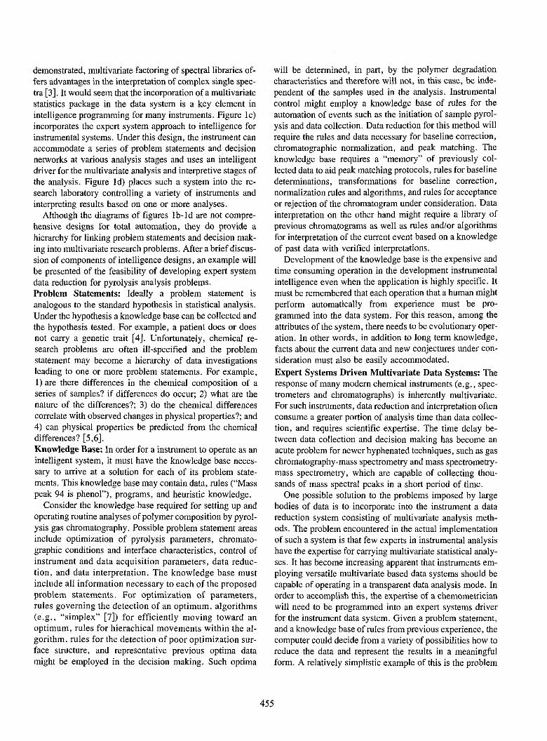
demonstrated, multivariate factoring of spectral libraries of-fers advantages in the interpretation of complex single spec-tra [3]. It would seem that the incorporation of a multivariatestatistics package in the data system is a key element inintelligence programming for many instruments. Figure ic)incorporates the expert system approach to intelligence forinstrumental systems. Under this design, the instrument canaccommodate a series of problem statements and decisionnetworks at various analysis stages and uses an intelligentdriver for the multivariate analysis and interpretive stages ofthe analysis. Figure Id) places such a system into the re-search laboratory controlling a variety of instruments andinterpreting results based on one or more analyses.

Although the diagrams of figures lb-Id are not compre-hensive designs for total automation, they do provide ahierarchy for linking problem statements and decision mak-ing into multivariate research problems. After a brief discus-sion of components of intelligence designs, an example willbe presented of the feasibility of developing expert systemdata reduction for pyrolysis analysis problems.Problem Statements: Ideally a problem statement isanalogous to the standard hypothesis in statistical analysis.Under the hypothesis a knowledge base can be collected andthe hypothesis tested. For example, a patient does or doesnot carry a genetic trait [4]. Unfortunately, chemical re-search problems are often ill-specified and the problemstatement may become a hierarchy of data investigationsleading to one or more problem statements. For example,I) are there differences in the chemical composition of aseries of samples? if differences do occur; 2) what are thenature of the differences?; 3) do the chemical differencescorrelate with observed changes in physical properties?; and4) can physical properties be predicted from the chemicaldifferences? [5,6].Knowledge Base: In order for a instrument to operate as anintelligent system, it must have the knowledge base neces-sary to arrive at a solution for each of its problem state-ments. This knowledge base may contain data, rules ("Masspeak 94 is phenol"), programs, and heuristic knowledge.

Consider the knowledge base required for setting up andoperating routine analyses of polymer composition by pyrol-ysis gas chromatography. Possible problem statement areasinclude optimization of pyrolysis parameters, chromato-graphic conditions and interface characteristics, control ofinstrument and data acquisition parameters, data reduc-tion, and data interpretation. The knowledge base mustinclude all information necessary to each of the proposedproblem statements. For optimization of parameters,rules governing the detection of an optimum, algorithms(e.g., "simplex" [7]) for efficiently moving toward anoptimum, rules for hierachical movements within the al-gorithm, rules for the detection of poor optimization sur-face structure, and representative previous optima datamight be employed in the decision making. Such optima

will be determined, in part, by the polymer degradationcharacteristics and therefore will not, in this case, be inde-pendent of the samples used in the analysis. Instrumentalcontrol might employ a knowledge base of rules for theautomation of events such as the initiation of sample pyrol-ysis and data collection. Data reduction for this method willrequire the rules and data necessary for baseline correction,chromatographic normalization, and peak matching. Theknowledge base requires a "memory" of previously col-lected data to aid peak matching protocols, rules for baselinedeterminations, transformations for baseline correction,normalization rules and algorithms, and rules for acceptanceor rejection of the chromatogram under consideration. Datainterpretation on the other hand might require a library ofprevious chromatograms as well as rules and/or algorithmsfor interpretation of the current event based on a knowledgeof past data with verified interpretations.

Development of the knowledge base is the expensive andtime consuming operation in the development instrumentalintelligence even when the application is highly specific. Itmust be remembered that each operation that a human mightperform automatically from experience must be pro-grammed into the data system. For this reason, among theattributes of the system, there needs to be evolutionary oper-ation. In other words, in addition to long term knowledge,facts about the current data and new conjectures under con-sideration must also be easily accommodated.

Expert Systems Driven Multivariate Data Systems: Theresponse of many modern chemical instruments (e.g., spec-trometers and chromatographs) is inherently multivariate.For such instruments, data reduction and interpretation oftenconsume a greater portion of analysis time than data collec-tion, and requires scientific expertise. The time delay be-tween data collection and decision making has become anacute problem for newer hyphenated techniques, such as gaschromatography-mass spectrometry and mass spectrometry-mass spectrometry, which are capable of collecting thou-sands of mass spectral peaks in a short period of time.

One possible solution to the problems imposed by largebodies of data is to incorporate into the instrument a datareduction system consisting of multivariate analysis meth-ods. The problem encountered in the actual implementationof such a system is that few experts in instrumental analysishave the expertise for carrying multivariate statistical analy-ses. It has become increasing apparent that instruments em-ploying versatile multivariate based data systems should becapable of operating in a transparent data analysis mode. Inorder to accomplish this, the expertise of a chemometricianwill need to be programmed into an expert systems driverfor the instrument data system. Given a problem statement,and a knowledge base of rules from previous experience, thecomputer could decide from a variety of possibilities how toreduce the data and represent the results in a meaningfulform. A relatively simplistic example of this is the problem

455

statement "Is there a correlation between two independentvariables?" Invisible to the user would be the operations fordetermining the integrity of the variable distributions, acomputation of the correlation and a determination of thesignificance of the correlation coefficient of the relation-ship. The result might take a simple form such as "thereappears to be a significant correlation between the first vari-able and the logarithm of the second variable. Would youlike to see the computed values?"

Demonstration of Expert System for DataAnalysis in Curie-point Pyrolysis

Mass Spectrometry

Pyrolysis mass spectrometry has come to the attention ofboth mass spectrometrists and chemometricians because ofits utility in the analysis of polymeric materials and thecomplexity of the mass spectra produced by natural poly-mers and biopolymers. The technique involves degradationof the solid material by pyrolysis followed by mass spec-trometry of the pyrolysis fragments. It has been demon-strated by the pioneering work of Meuzelaar (for examplesee [8]) that Curie-point pyrolyses of samples of biomateri-als can produce profiles which, when properly normalized[2], are reproducible and diagnostic of the chemical similar-ities and dissimilarities among groups of samples and arequantitative under appropriate experimental designs [9]. Be-cause the process of pyrolysis followed by mass spectrome-try of the network polymer of natural heterogeneous bio-polymers produces mass spectra with peaks which tend to behighly correlated, the interpretation problems createdby the vast number of, and the overlap of, the masses aresolved through multivariate analysis of the mass spectralprofiles. A data system for a pyrolysis mass spectrometerwould be of limited utility without multivariate statisticalmethods [2].

To test the hypothesis that an expert systems approach todata reduction is potentially helpful and feasible, an expertsystems driver was implemented to mimic the data analysisportion of a Rocky Mountain Coal study done at Biomateri-als Profiling Center in Utah. Detailed results of the originalstudy can be found in [5,6] and of the numerical methodsused in [2]. Briefly, 102 Rocky Mountain Coals were ana-lyzed in quadruplicate by pyrolysis mass spectrometry. Thepyrolysis profiles were added to a preexisting data set con-taining conventional measurements on the same coal sam-ples (see table 1). After normalization of the profiles by themethod of Eshwis et al. [10], average mass specta wereanalyzed using multivariate analysis techniques.

Figure 2 is a minimal design for an expert systems driven

data acquisition and analysis system for pyrolysis massspectrometry. Figure 3 shows the design of the data basesfor the present application. As diagrammed in figure 2, each

Table 1. Conventional measurement contained in the "old data" database for the Rocky Mountain coals.

Conventional Measurements

Vitrinite % PotassiumFusinite % PhosphorusSemifusinite % MoistureMacrinite % Pyritic sulfurLiptinite % Mineral matterVitrinite Reflectance % Volatiles% Silicon % Organic sulfur% Aluminum Calorific value% Titanium % Organic carbon% Magnesium % Organic hydrogen% Calcium % Organic sulfur% Sodium % Organic nitrogen

% Organic oxygen

operation of the instrument requires an expert systems driverand decision module for its automation. A rudimentary ex-pert systems was built to mimic the decision making usedfor statistical analysis of coal pyrolysis patterns. This sys-tem demonstrates the problems and pitfalls associated withintelligent instrumental development.

Normalization is rarely an option in pyrolysis techniquessince the size of the sample undergoing electron impact isdetermined by the quantity of pyrolsates actually makingtheir way to the ion source of the mass spectrometer. Forthis reason, spectra are normalized to place each sample ona relative quantitative basis. Furthermore, when replicatesof a single sample are analyzed in detail, it is found thatsome peaks replicate better than others. For example, if anorganic solvent is used during the sample preparation, themass peaks due to this solvent replicate poorly. The same istrue of contaminants absorbed to the sample matrix. On theother hand, because the sample size in terms of total ioncounts is a variable in these experiments, often one or morereplicate spectra will exhibit outlying tendencies when com-pared to other replicates of the same sample.

NORMA [2], developed by Meuzelaar's group at Utah, isdesigned to select peaks with stable variance characteristicsfor inclusion in the normalization process. With this routinean expert interacts with the computer in a loop of peakdeletions and replicate spectra deletions until a set of peaksis defined which stabilizes the normalization process.

An expert systems approach to the software interactionrepresents peaks by their variances over the samples andsample replicates and spectra by Euclidean distances be-tween replicates over the mass units. A library data base fornormalization is established which contains spectra patternsfor commonly used solvents and commonly encounteredcontaminates as well as the background spectrum from themass spectrometer. The expert sysems are initialized bycomputation of peak variances. The variances are orderedhigh to low andthe shape of the plot of ordered variances is

456

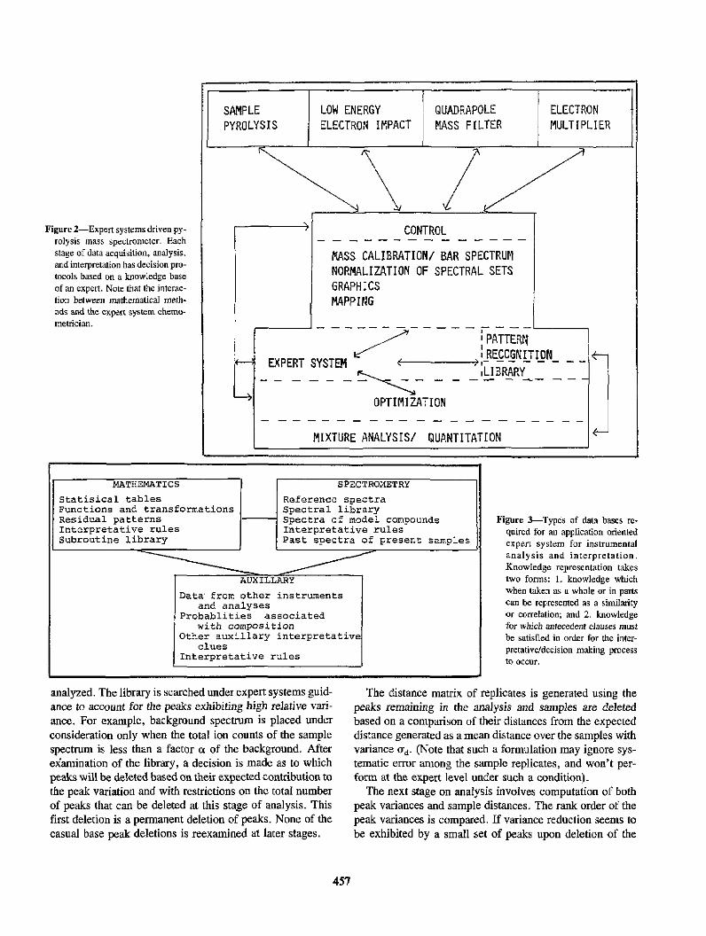
Figure 2-Expert systems driven py-rolysis mass spectrometer. Eachstage of data acquisition, analysis,and interpretation has decision pro-tocols based on a knowledge baseof an expert. Note that the interac-tion between mathematical meth-rds and the expert system chemo-metrician.

K

EXPERT

QUADRAPOLE

MASS FILTER

ELECTRON

MULTIPLIER

CONTROL

MASS CALIBRATION/ BAR SPECTRUM

NORMALIZATION OF SPECTRAL SETS

GRAPHICS

MAPPING

PATTERN

* SYSTEM a , ,RECCGNITION_- - -US- ~'- --- - -- - --SYSTEI N LIBRARY

OPTIMIZATION

MIXTURE ANALYSIS/ QUANTITATION

MATHEMATICS

Statisical tablesFunctions and transformationsResidual patternsInterpretative rulesSubroutine library

SPECTRONETRY

Reference spectraSpectral librarys spectra of model compoundsInterpretative rulesPast spectra of present samples

Figure 3-Types of data bases re-quired for an application orientedexpert system for instrumentalanalysis and interpretation.Knowledge representation takestwo forms: 1. knowledge whichwhen taken as a whole or in panscan be represented as a similarityor correlation; and 2. knowledgefor which antecedent clauses mustbe satisfied in order for the inter-pretativedecision making processto occur.

analyzed. The library is searched under expert systems guid-ance to account for the peaks exhibiting high relative vari-ance. For example, background spectrum is placed underconsideration only when the total ion counts of the samplespectrum is less than a factor at of the background. Afterexamination of the library, a decision is made as to whichpeaks will be deleted based on their expected contribution tothe peak variation and with restrictions on the total numberof peaks that can be deleted at this stage of analysis. Thisfirst deletion is a permanent deletion of peaks. None of thecasual base peak deletions is reexamined at later stages.

The distance matrix of replicates is generated using thepeaks remaining in the analysis and samples are deletedbased on a comparison of their distances from the expecteddistance generated as a mean distance over the samples withvariance d. (Note that such a formulation may ignore sys-tematic error among the sample replicates, and won't per-form at the expert level under such a condition).

The next stage on analysis involves computation of bothpeak variances and sample distances. The rank order of thepeak variances is compared. If variance reduction seems tobe exhibited by a small set of peaks upon deletion of the

457

AUXILLARY

Data from other instrumentsand analyses

Probablities associatedwith composition

Other auxiliary interpretativeclues

Interpretative rules

SAMPLE LOW ENE

PYROLYSIS ELECTR(

V"��

-.RGY

)N IMPACT

samples, the peaks involved are temporarily deleted, thesamples previously deleted are brought back into analysisand the distances reexamined. The expert systems decidewhich will be deleted at this stage, peaks or samples basedon the recomputed distances. The iterative decision mak-ing-statistical computation continues until a key set ofpeaks remain activated for normalization over all spectra. Adiagram of the proposed normalization experts system isshown in figure 4.

The system, as described, does not completely emulate anexpert for all applications of pyrolysis mass spectrometry. Ithas already been noted that the data evaluation does notaddress errors which arise from time dependent or system-atic error. In addition to this, the decision making process,while designed to emulate the human decision process basedon statistical results, does not necessarily operate on a one-to-one correspondence with a human expert. The problem isthat two experts working on the same set of data may arriveat approximately the same results via slightly different pro-cedural routes. The same is true of the expert system whencompared to a human expert. The major deviations from a

-

nextiteration

I~1

I

I

1i

3-~ | Normalization of spectra I

i convergenceQuit and save normalization

Figure 4-Interaction of expert systems and statistical computation for arational normalization process for pyrolysis mass spectrometry.

human procedure found when working with this system isthe lack of "intuition" or "fuzzy logic" that is used by theexpert. The expert systems converges in more steps than isnecessary by human interaction with the statistical al-gorithms and for some data bases, has trouble defining con-vergence at the solution. For example, the optimal cut offparameters for variance and distance change between datasets. These and other problems are best solved by trainingthe expert systems to recognize the structure of a goodspectal solution in addition to the structure of good statistics.

Correlation Based Hypothesis Testing

Perhaps the most often asked question of large data setsinvolves finding relationships between the variables or be-tween the variables and an external parameter. Table 2 liststhe form of the problem statements included in our datasystem for this demonstration. The term "relate" invokesone of several multivari ate algorithms for the study of corre-lations in the data. The possible responses are the Pearsoncorrelation coefficient, linear regression, factor analysis orcanonical correlation analysis.

Consider the problem statement: What is the relationshipof peak 34 (H2S) in the mass spectrum of coal to the totalorganic sulfur from the conventional data matrix. "Relatecurrent data, mass 34 to old data, organic sulfur over sam-ples, all" results in a computation of the correlation coeffi-cients, a estimate of significance and the confidence intervalabout the correlation. "Relate current data, mass 34 to olddata, organic, sulfur over samples, all; Interprete using olddata, organic sulfur" results in the additional computationof (organic sulfur)=a (mass 34)+b with residuals Ej. Theresidual pattern is tested for randomness. A failure results ina search through the library for a reference residual patternwith similarities to the computed residual pattern.

The next relate function asks for a study of the relation-ships among variables in the current data set. "Relate cur-rent data, all with current data, all over samples, all"results in the factor analysis of the data correlation matix.The loadings of the factor analysis are interpreted for thevariable relationships seen along the orthogonal axes of theoriginal rotation. This interpretation is an experts systemsbased analysis of the major peak series and will be discussedlater.

Interpretation of the factor score is a difficult problem.Consider the two dimensional factor score projection ofthese data. Figure 5a is a projection without labels. Figure5b is the same projection after a human expert has assignedsample labels corresponding to the geological source of thesamples and an interpretation. Figure Sa is representative ofthe information about the factor scores stored by the com-puter. The addition of labels is readily accomplished but,without training, patterns formed by the sample labels

458

Program InitializationSelect samplesSort if necessaryEvaluate ion intensities

Compute mass variancesa. over all samplesb. within replicatesComputte sample distancesa. over all samplesb. within replicatesSort all statisticsForm F-statistic ratios

Expert system evaluationa. of mass variationsb. of sample distances

Expert system decisionsa. delete mass peaksb. delete samplesc. reactivate mass peaksd. reactivate samples

Table 2. Variations of the expert system commands RELATE and INTERPRETE USING. The FORTRAN subroutine calling protocols arebased on the data types used in each variable location of the command and on the command sequence. Note that the same command stringsand rotes cm accomodate computation on questions about the data base transpose matrix when ".OVER samples ... " is replaced by"..OVER variables..."

RELATE data base t, variable list I TO data base 2, variable list 2 OVER samples, sample list

Examples:

1. RELATE current data, mass 34 TO old data, organic sulfur OVER samples, match(Results: correlation coefficient and significance test)

2. RELATE current data, mass 34 TO old data, organic sulfur OVER samples, match; INTERPRETE USING old data, organic sulfur(Results: correlation computed at least squares fit, significance test, and residual pattern evaluation)

3. RELATE current data, all TO current data, all OVER samples, all(Results: Factor analysis of current data and loading interpretation)

4. RELATE current data, all TO old data, calorific value OVER samples, match, active; INTERPRETE USING old data, calorific value(Results: Factor analysis of current data followed by target rotation to calorific value and interpretation of loadings)

5. RELATE current data, all TO old data, all OVER samples, match(Results: Canonical correlation analysis of two data bases and interpretation of mass spectral loadings)

within the space have little meaning. A generalized solution (a)to this problem does not seem likely. Each study would *

require an elaborate knowledge base specific to the samples *

in order to interpret trends seen in this picture.For the coal data, the old data matrix of conventional

measurements provides a more easily implemented route for ,hypothesis testing on the pyrolysis mass spectral factors.Consider once more the "relate" command. After matchingthe two data sets by the logic used in [5], factor analysis ofthe PY/MS set followed by "Relate current data 2, all with 0.0- - so

old data, calorific value using samples, active; interpret c 'Cusing old data, calorific value" results in the regression *analysis of calorific value=E W (factor scores)py-.T+b pro-ducting both the variable and the sample relationships of the -l0rotation of the Py/MS data to calorific value. The results are s . .given in figure 6 and discussed in [6]. 42 0 0.D 1.0

The last example of a correlation based statement is 2.D- -

"Relate current data, all with old data, all over samples, CANIEL ball." This results in a cannonical correlation analysis factor- 'KING

ing both data matrics in such a way that the overlap ininformation between the sets is maximized. Four factors are -. -

extracted. The first two of these are shown in figures 7 a o

through 9. This analysis showed these data sets to be ap-suBBIrproximately 80% correlated over the coal samples. The r doe a _ -.

major chemistry of the conventional measurement trends aregiven above the spectral representation form the Py/MS - -

factors. Z OS^ , _

Figure S-Comparison of computer representation of factor scoes (a.) to c . OA'

the same plot after interpretation by an expert (b.) Symbols represent X _ .- -¶sample specific relationships deduced by the expert. Dotted lines are a B ' U * UPPERseparation of the samples into classes not available to the computer in the cto.pyrolysis data base. The knowledge base required to mimic the expert ,would form a reference book of information about the samples. The 4.o -1.0 0.0 D.0

generation of such a knowledge base would be a fonritable task. FACTOR I SCORE

459

naphthaIenes-05 ie0

.7'alkenes alkyl fragments ' - - _28 56 / 6

±s(C jj) 2 5 ° Il

30 40 50 70 ~00 0 0 2 3 40 50I 0 90 Z0OO 7

IS ~~148 INS 17se0 62 naphthols

01 1 12~~~~~~~~~ i2indancolsketones benzene phenol -| benzolurans (indanes)

carboxy acids dihydroxybenzenes(aIcohols)

Figure 6-Chemical interpretation of the mass spectral peaks associated strongly with a targeted least squares rotation of pyrolysis factor scores tothe external parameter calorific value. Peak interpretations were accomplished by the system described in figure 10. Results on chemicalinterpretation are identical to those of the original study, demonstrating that chemical infonnation is more readily implimented as an expert systemthan sample specific information for this instrumental method.

R(ZAcXc) = R(ZAPXP) = 0.99

R(ACXCJAPXP) = 0,95

CONVENTIONAL MEASUREMENT SET

CALORIFIC VALUE -

ORGANIC OXYGEN +

MOISTURE +

ORGANIC CARBON -REFLECTANCE -

PYROLYSIS MASS SPECTRAL DATA SET

1681 3,-. 114~2'_. a 1 1N I P AEg

I's 70 184 NAPHrtEEI T "'I' `T'' "*' Ir

M/Z 40 50 60 10 80 90 100 510 120 130 140 150 160 170 IN3 190 200 210 220 230

Figure 7-First canonical variate loadings for the rotation of pyrolysis mass spectra of coal samples to the conventional data matrix described intablet. The correlation of the data bases to the derived variate (Z) is 0.99 and to each other is 0.95. A0Xc and APXP are the linear composites ofthe conventional and pyrolysis data bases respectively. Only the signs of the strongly correlated variables of the conventional data are given.Loadings for the pyrolysis data are given as positive and negative. Interpretations of mass peak were accomplished using the system described infigure 10.

460

C-ti

56ALKENES

R(ZAcXc) = R(ZAPXP) = 0.96R(ACXCiAPXP) = 0.86

CONVENTIONAL MEASUREMENT SET

SEMIFUSINITE -

SODIUM +

VOLATILES +

REFLECTANCE -

PYROLYSIS MASS SPECTRAL DATA SET

ISOPRENOID SIGNALS ?

41 DIENES 79 TRIENES 1 as 202'41 OlDIES ~ ~ 9 159 173E69 F 119 133 Ihi! ~~~~131r

*~~~~~~~~~~ ~~~~~~ tK _ l 1_ __ _ a a ' 11 ll 1 .1, ,

1S t20 5'4 16 8 [} IYDROXY-

92 a 12 \ L / i'96 tt 210FLUOREWES

NAPXTHALEIIES IE/ j (HEANTa4ENEsAX FLUORENES

/NT58RACEE 1 3 I/

L,/Z410 50 60 70 80 90 100 010 120 130 140 150 160 170 1 0 10 200 210 220 230

Figure S-Second canonical variate loadings for the rotation of pyrolysis mass spectra to the conventional data matrix described in table 1. See figure7 for an explanation of the symbols used in this figure. Interpretation by the system described in figure 10 failed for the positive loadings labeledas isoprenoid signals?. These were assigned by the authors.

Figure 9-Canonical variate scoreson the first two axes (described infigs. 7 and 8). Dotted lines separat-ing classes were inserted by the an-thors and not interpreted by the ex-pert system (see fig. 5 for anexplanation of implimentation -

problem for sample interpretation.)

HIGHVOLATILEBITUMINOUS,

A

I.

: 0

/ I* 1

*11 0. *0

0

0 0

** | @ - @0.8

%. atL *.0* :0

S 0SOD _ -*

. #0* :00

.

0HIGH VOLATILEBITUMINOUS B

00

0

I SUBBITUMINOUS

*I

HIGH VOLATILE BITUMINOUSC

FIRST CANOnICAL COMPONENT

461

II

i

I

I

i

II

I

I

I

The assignment of chemical interpretations for mass spec-tra and for factor loadings is accomplished by an expertsystems intepreter that can be used for any study in whichthe samples are coal. The data base for the interpretationincludes commonly encountered chemical species in coal,the major peaks expected from their presence and, given twochemical species with similar patterns, the probability oftheir contribution as a major component to a coal pattern.Also included is a routine for generating molecular speciesfrom C,N,O, and S given the base peak molecular weightand the ion series. The operation of the expert system alongwith the results of each iteration are given in figure 10.Because Py-MS spectra contain many low intensity massesof questionable interpretation, and because factor loadingsare rarely pure, only the most intense ion series patterns areinterpreted. The program is initialized by setting an initialthreshold limit (TL3). The ions (m/z) above the thresholdare collected, sorted and given temporary chemical assign-ments. The threshold limit is lowered each time by a lesserfactor until it encounters the "grassy" region of the spec-trum. At this point, permanent ion series interpretations areassigned. The "?" appearing in the figure for Mass 104means that no library interpretation of this peak was foundand that the number of peaks in the ion series was below thelimit set for generation of hypothetical molecular species.The entire system is diagramed in figure 11.

a

3

TI)3 40 60 80 100 VO 140 160 180 200 220

COLLECTED MASSES: 2a .2 C2 H494 £7810 C6S6O

110 C8H14 , £6H602

SORTED MASSES: 28, 42 CN"94.108 C 2N-4

110,124 C2-

(TI 12

SORTED PASSES:

(TIoSORTED MASSES:

BASE MASS

28, 4294.:08.122

110.124

26. 42. 56. 7032344468. 02

SERIES

42 C3H5I10 Cg112 , C7 H8D124 CgN16 , C/HuOG

4 (c66)OCNH

5. (C656)02Ct HN

(TI)i

28, 42. 563234

94, t10,122110,124,139

92.105,120,134,148,16294,106.122, 136

104120,124,138132. 146.160158

PRIMARY ASSIGNKENT

Discussion

The correlation work described in this paper along withsimilar considerations of other algorithms seem to supportthe possibility that, for a given instrument, an expert sys-tems driver for data analysis can be developed which isindependent of the nature of the chemical problem. The wayto accomplish this is to build expert systems drivers tointerpret the problem statement and to interpret the dataanalysis results. Viewed in this manner, an instrument-dependent expert system can generate the experimental de-sign and optmization from the problem statement and passto the data analysis driver the statistical elements necessaryfor its decision on the proper data reduction protocol. Learn-ing is initiated when the data analysis system receives anunrecognizable set of elements. Otherwise, the expert sys-tem selects from the knowledge base the algorithm sequencefor data reduction.

We are currently extending these concepts to the con-struction of an expert system, EXMAT, for experimentaldesign, optimization, data reduction and interpretation ofmeasurements made on a sample by a variety of thermalanalysis instrumental techniques. TIMM® (General Re-search Corp., Mclean, VA) a FORTRAN-based expertsystem generator, has been enabled development of aheuristically-linked set of expert systems for material analy-

20

32

34

444

88

92

944

28. 42. 56, 70

32

34

44

68. 82

92,106,120.1341148,162

94,108.122.136

104 104

110 110.124,138

132

158

132.146.160

C4H2N ALKENE

CN 2s.20 ALCtHOLH2S

CI.2842 ALJANE

C H2T-2 D I ENE

( )C8 II2 ,ALY _L- BENZENE

(05p44)C4H2,.,10H

ALKYL-PHENOL

(C6s3)CHsH2(102H2DIHYeDOXYBENZENE

IMOMS-BENZOFURANS

NAPMOh0LS.INDENES

Figure 10-Operation of the expert system used to interprete the pyrolysismass spectra and spectral loadings in the demonstration. The rules usedto sort and interprete the peaks are based on ion series produced by massdifferences of 14 (CH2 ). Base peaks help terminate series for resolutionof multiple interpretations. ? is a peak not present in the data base.

sis. The attributes of the TIMM® system are listed in table3. In order to accomplish the analytical goals of this project,we have combined the concepts of specific instrumentalintelligence with the goals set forth in figure la to providea data system capable of experimental designs utilizing oneor several analysis techniques. Each instrument retains itsown control, design, preprocessing and interpretative expertsystems unit but the data analysis unit has, of necessity,been generalized for analysis of data from a single or from

462

Figure 11-Steps in the expert sys-tem interpretation on pyrolysismass spectra of coals.

I SET ~THRESHOL~D I ICOLLECT PEAKS SORT PEAKS FORIIN (T) maxALKYL LOSS I

SEARCH RULES|COLTPEKFOR INTZRPRETATION Ia IN NEXT TI

I not found / ast TI| GENERIATE FORMULA-S k|EIIAE[ IDSS GENTE |Ca Ib0c d e PEK 1FINALLS A STRUCTURES[

Table 3. Attributes of the TIMMR expert system. TIMMR was adapted to our application because addition of FORTRAN subroutine librarycalls is more readily accomplished than in other systems and because the decision logic can already use computationally based rules aswell as chaining logic rules.

TIMMR: A FORTRAN - BASED EXPERT SYSTEMS APPLICATIONS GENERATOR, General Research Corporation

Forwardlbackward chaining using analog rather than propositional representation

Knowledge base divided into two sections: declarative knowledge and knowledge body

Pattemn-matching using a nearest neighbors search algorithm to compare cunent situation with antecedent clauses

Unique similarity metric computed form order information in declarative knowledge giving distance metric over all classes

Decision structure and knowledge body readily developed and modified by expert in any domain

Heuristically-linked expert system using implicit and explicit method permitting processing of "microdecisions' that are pan of"macrodecisions"

Each system independently built, trained, exercised, checked for consistancy and completeness and then generalized

multiple measurement techniques. Table 4 gives a outline ofthe decision making process for the experimental designexpert system, and for data interpretation. Rule generationunder the system is demonstrated in figure 12. The expertsystem strategy for the chemometrics portion of the systemis similar to that described previously in the Py-MS example

with the added feature that the system generate the protocolof analysis based on the initial problem statement and theavailable data. The system is in its earliest stages of devel-opment so any or all aspects of the proposed design aresubject to modifications as experience is gained in trainingthe system. Nevertheless, we feel that an expert systemssuch as ours offers a strategy for automation of laboratoryinstrumentation and interpretation under an expert systemsapproach.

Rule IIf:

SCOPE IS R&DSAMPLE AMT IS TRACESAMPLE FORM IS POWDERSAMPLE PROCESS IS *SAMPLE HISTORY IS *INSTR. AVAIL IS ALL

Then:ANAL STRATEGY IS SPECTRMS(1.0)

Figure 12-Example of rule generation in EXMAT using the TIMM®expert system. Rule is from the expert system for analytical strategy.

Table 4. Example taken from overall organization structure ofEXMAT, an expert systems for materials analysis.

ANALYTICAL STRATEGY DATA INTERPRETATON

CHOICES: CHOICES:CHROMGC PATTERN RECOGNITIONCHROMLC SAMPLE IDSPECTRFTIR GROUP IDSPECTRMS PEAKS IDTHERMTA NO IDELEMEL COMBINE DB

EXTEND DBCORRELATION

FACTORS: FACTORS:I. SCOPE I. DATA GENERATE

QUAL FTIR DBQUANT MS DBPURITY LC DBQUALDQUANT TA DBTIME/FUND LIMIT GC-FTIR DBTRACE GC-MS DOR&D GC DBCORRELATION 2. GC DB TREATMENTSCREEN DIRECT COMPARE

CHEMOMETRICSDATA SET ID

3. FTIR DB TREATMENTDIRECT COMPAREPAIRS SEARCH

4. ETC. FOR EACHDATA BASE (DB)

463

References

[I] Harper, A.M., Polymer Characterization Using Gas Chromatographyand Pyrolysis, S. Liebman and EJ. Levy, Marcel Dekker, Inc.(1985).

[2] Harper, A.M.; H.C.L. Meuzelaar, G.S. Metcalf, and DL. Pope,Analytical Pyrolysis Techniques and Applications, K. Voorhees,ed. 157-195 (1984).

[3] Owens, P.M.; R.B. Lamb and T.L. Isenhour, Anal. Chem., 54 2344(1982).

[4] McMuny, I.E.; J.A. Pine, P.C. Jurs, B. Lavine, and A.M. Harper,Anal. Chem., vol. 57, 295-302 (1985).

[5] Meuzelaar, H.L.C., and A.M. Harper, Characterization and Classifi-cation of Rocky Mountain Coals by Curie-Point Mass Spectrome-try, Fuels, vol. 63, 639-652 (1984).

[6] Harper, A.M.; H.L.C. Meuzelaar, and P.H. Given, Fuels, vol. 63,793-799 (1984).

[7] Deming, S.N.; S.L. Morgan, and M.R. Willcott, American Labora-tory, October, 13 (1976).

[8] Meuzelaar, H.L.C.; J. Haverkamp, and FD. Hileman, Curie PointPyrolysis Mass Spectrometry of Recent and Fossil Biomaterials,Elsevier, Amsterdam (1982).

[9] Windig, W.; P.G. Kistemaker, and J. Haverkamp, J. Anal. Appl.Pyrol., 3, 199 (1982).

[10] Eshwis, W.; P.G. Kistemaker and H.L.C. Meuzelaar, AnalyticalPyrolysis, CER, Jones, ed., Elsevier, Amsterdam, 151-166

(1977).

DISCUSSIONof the Harper-Liebman paper, IntelligentInstrumentation

Richard J. BeckmanLos Alamos National Laboratory

There has been an instrumentation revolution in thechemical world which has changed the way both chemistsand statisticians think. Instrumentation has lead chemists tomultivariate data-much multivariate data. Gone are thedays when the chemist takes three univariate measurementsand discards the most outlying.

Faced with these large arrays of data the chemist canbecome somewhat lost in the large assemblage of multivari-ate methods available for the analysis of the data. It isextremely difficult for the chemist-and the statistician forthat matter-to form hypotheses and develop answers aboutthe chemical systems under investigation when faced withlarge amounts of multivariate chemical data.

Professor Harper proposes an intelligent instrument tosolve the problem of the analysis and interpretation of thedata. This machine will perform the experiments, formulatethe hypotheses, and "understand" the chemical systemsunder investigation.

What impact will such an instrument have on bothchemists and statisticians? For the chemist, such an instru-

ment will allow more time for experimentation, more timeto think about the chemical systems under investigation, a

better understanding of the system, and better statistical andnumerical analyses. There would be a chemometrician in

every instrument! For the statistician, the instrument willmean the removal of outliers, trimmed data, automated re-gressions, and automated multivariate analyses. Most im-portant, the entire model building process will be auto-mated.

There are some things to worry about with intelligentinstruments. Will the chemist know how the data have beenreduced and the meaning of the analysis? Instruments madetoday do some data reduction, such as calibration and trim-ming, and the methods used in this reduction are seldomknown by the chemist. With a totally automated system thechemist is likely to know less about the analysis than he doeswith the systems in use today.

The statistician when reading the paper of ProfessorHarper probably asks what is the role of the statistician inthis process? Will the statistician be replaced with a mi-crochip? Can the statistician be replaced with a microchip?In my view the statistician will be replaced by a microchipin instruments such as those discussed by Professor Harper.This will happen with or without the help of the statistician,but it is with the statistician's help that good statisticalpractices will be part of the intelligent instrument.

Professor Harper should be thanked for her view of thefuture chemical laboratory. This is an exciting time for boththe chemist and the statistician to work and learn together.

464

Journal of Research of the National Buieau of StandanisVolume 90, Number 6, November-December. 1985

The Regression Analysisof Collinear Data

John MandelNational Bureau of Standards, Gaithersburg, MD 20899

Accepted: July 1, 1985

This paper presents a technique based on the inuitively-simple concepts of Sample Domain and Effective PredictionDomain, for dealing with linear regression situations involving collinearity of any degree of severity. The EffectivePrediction Domain (EPD) clarifies the concept of collinearity. and leads to conclusions that are quantitative andpractically useful. The method allows for the presence of expansion tenms amongthe regressors, and requies no changeswhen dealing with such situations.

Key words: collinearity: efficient prediction domain; ill-conditioning; multicollinearity; regression analysis.

Introduction

The scientists' search for relations between measurableproperties of materials or physical systems can be effec-tively helped by the statistical technique known as multipleregression. Even when limited to linear regression, the tech-nique is often of great value, as we shall see below. Often,however, difficulties in interpretation arise because of acondition called collinearity. This condition, which is inher-ent in the structure of the design points (the X space) of theregression experiment, is often treated, at least implicitly, asa sort of disease of the data that is to be remedied by specialmathematical manipulations of the data.

We consider collinearity not as a disease but rather asadditional information provided by the data to the data ana-lyst, warning him to limit the use of the regression equationas a prediction tool to specific subspaces of the X space, andtelling him precisely what these subspaces are. Thus,collinearity is an indication of limitations inherent in thedata. The statistician's task is to detect these limitations andto express them in a useful manner. If this viewpoint isadopted, there is no need for remedial techniques. All thatis required is a method for extracting the additional informa-tion from the data. We will present such a method.

The Model

We assume that measurements y have been made at anumber of "x-points," each point being characterized by thenumerical values of a number of "regressor-variables" xj.We also assume that y is a linear function of the x -variables.The mathematical model, forp regressors, is:..=PXI+PX2+- .+PXj+. ..+ppxp+E(1)

where E is the error in the y measurement. We denote by N

the number of points, or "design points", i.e., the combina-tions of the x's at which y is measured.

Usually, the variable xl is identically equal to "one" forall N points, to allow for the presence of a constant term.Then the expected value of y, denoted E(y), is equal to fi1when all the otherx 's are zero. This point, called the origin,is seldom one of the design points and is, in fact, quite oftenfar removed from all design points. In many cases this pointis even devoid of physical meaning.

First Example:Firefly Data

We present the problem in terms of two examples of realdata. The first data set (Buck [IIl) is shown in table 1. Itconsists of 17 points and has two regressors, in addition to

Figures in brackets indicate literature references.

465

About the Author: John Mandel is a statistical con-sultant serving with NBS' National Measurement Labo-ratory.

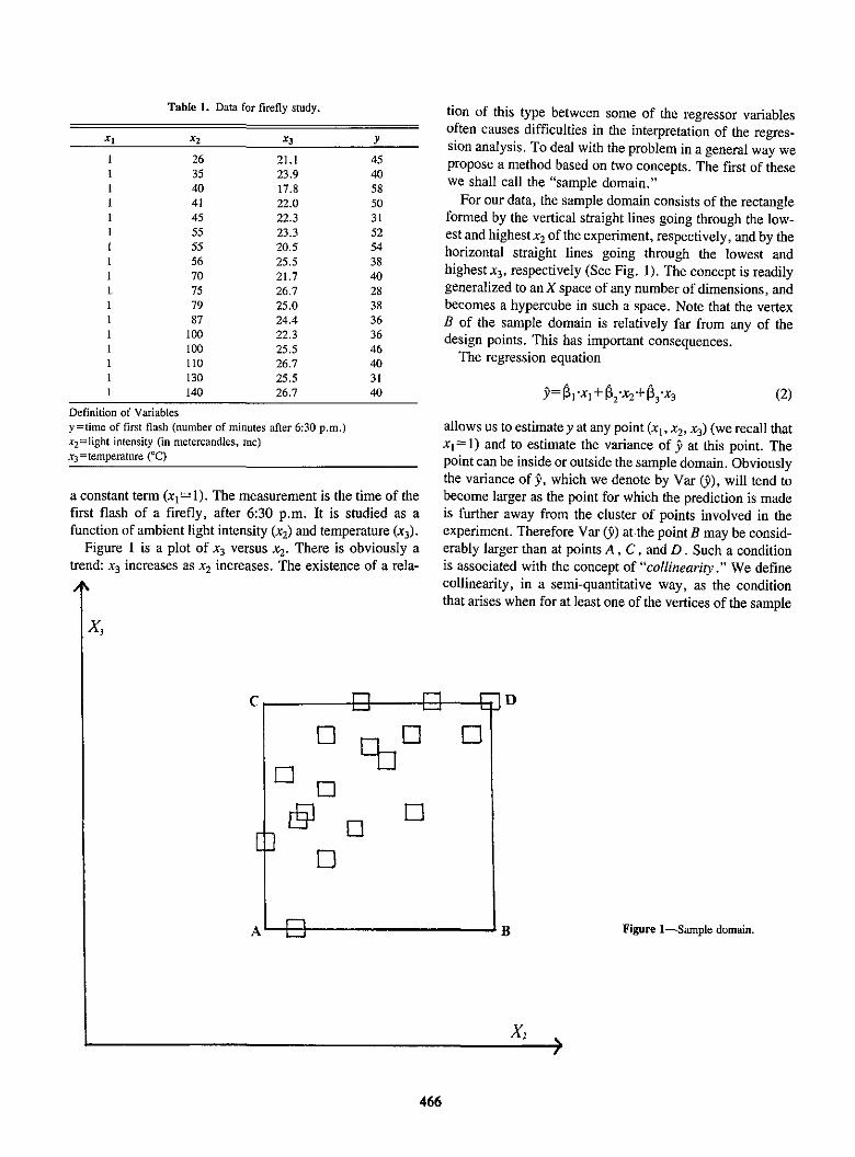
Table 1. Data for firefly study.

x1 x2 X3 y

1 26 21.1 451 35 23.9 401 40 17.8 581 41 22.0 501 45 22.3 311 55 23.3 521 55 20.5 541 56 25.5 381 70 21.7 401, 75 26.7 281 79 25.0 381 87 24.4 361 100 22.3 361 100 25.5 461 110 26.7 401 130 25.5 311 140 26.7 40

Definition of Variablesy =time of first flash (number of minutes after 6:30 p.m.)x2 =ight intensity (in metercandles, me)xr=temperature (0 C)

a constant term (xlea 1). The measurement is the time of thefirst flash of a firefly, after 6:30 p.m. It is studied as afunction of ambient light intensity (x2) and temperature (x 3).

Figure I is a plot of X3 versus x2. There is obviously atrend: X3 increases as x2 increases. The existence of a rela-

A%

tion of this type between some of the regressor variablesoften causes difficulties in the interpretation of the regres-sion analysis. To deal with the problem in a general way wepropose a method based on two concepts. The first of thesewe shall call the "sample domain."

For our data, the sample domain consists of the rectangleformed by the vertical straight lines going through the low-est and highest x2 of the experiment, respectively, and by thehorizontal straight lines going through the lowest andhighest X3 , respectively (See Fig. 1). The concept is readilygeneralized to an X space of any number of dimensions, andbecomes a hypercube in such a space. Note that the vertexB of the sample domain is relatively far from any of thedesign points. This has important consequences.

The regression equation

5=IVlx,+0 2 .X 2+03.x 3 (2)

allows us to estimate y at any point (xl, x2, X3 ) (we recall thatxi= 1) and to estimate the variance of 9 at this point. Thepoint can be inside or outside the sample domain. Obviouslythe variance of 9, which we denote by Var (9), will tend tobecome larger as the point for which the prediction is madeis further away from the cluster of points involved in theexperiment. Therefore Var () at the point B may be consid-erably larger than at points A, C, and D. Such a conditionis associated with the concept of "collinearity." We definecollinearity, in a semi-quantitative way, as the conditionthat arises when for at least one of the vertices of the sample

x3

C

A

2 E] c] ED

B Figure I-Sample domain.

X 2

I,

466

B1E31 ] DUE

. 71

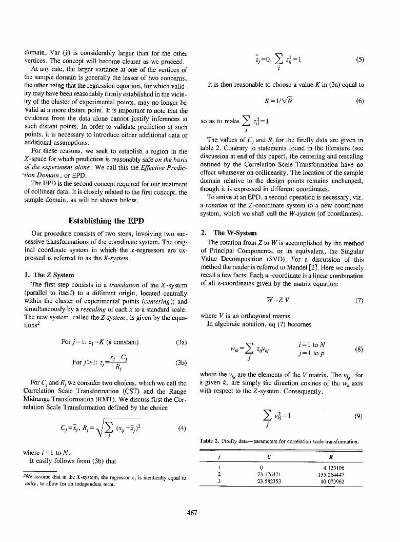
domain, Var (9) is considerably larger than for the othervertices. The concept will become clearer as we proceed.

At any rate, the larger variance at one of the vertices ofthe sample domain is generally the lesser of two concerns,the other being that the regression equation, for which valid-ity may have been reasonably firmly established in the vicin-ity of the cluster of experimental points, may no longer bevalid at a more distant point. It is important to note that theevidence from the data alone cannot justify inferences atsuch distant points. In order to validate prediction at suchpoints, it is necessary to introduce either additional data oradditional assumptions.

For these reasons, we seek to establish a region in theX-space for which prediction is reasonably safe on the basisof the experiment alone. We call this the Effective Predic-

'tion Domain, or EPD.The EPD is the second concept required for our treatment

of collinear data. It is closely related to the first concept, thesample domain, as will be shown below.

Establishing the EPDOur procedure consists of two steps, involving two suc-

cessive transformations of the coordinate system. The orig-inal coordinate system in which the x-regressors are ex-pressed is referred to as the X-system.

1. The Z System

The first step consists in a translation of the X-system(parallel to itself) to a different origin, located centrallywithin the cluster of experimental points (centering); andsimultaneously by a resealing of each x to a standard scale.The new system, called the Z-system, is given by the equa-tions2

j = Z0, E Z32= 1 (5)

It is then reasonable to choose a value K in (3a) equal to

K=I/VN (6)

so as to make Z21=1

The values of Cj and Rj for the firefly data are given intable 2. Contrary to statements found in the literature (seediscussion at end of this paper), the centering and rescalingdefined by the Correlation Scale Transformation have noeffect whatsever on collinearity. The location of the sampledomain relative to the design points remains unchanged,though it is expressed in different coordinates.

To arrive at an EPD, a second operation is necessary, viz.a rotation of the Z-coordinate system to a new coordinatesystem, which we shall call the W-system (of coordinates).

2. The W-System

The rotation from Z to W is accomplished by the methodof Principal Components, or its equivalent, the SingularValue Decomposition (SVD). For a discussion of thismethod the reader is referred to Mandel [2]. Here we merelyrecall a few facts. Each w -coordinate is a linear combinationof all z-coordinates given by the matrix equation:

W=Z V (7)

where V is an orthogonal matrix.In algebraic notation, eq (7) becomes

For j = 1: z1 =K (a constant)

Forj>l: Zji= ci

For Cj and Ri we consider two choices, which we call theCorrelation Scale Transformation (CST) and the RangeMidrange Transformation (RMT). We discuss first the Cor-relation Scale Transformation defined by the choice

(4)

where the vki are the elements of the V matrix. The vkj, fora given k, are simply the direction cosines of the wk axiswith respect to the Z-system. Consequently,

2 = I

Cjxij, Rj -(9)I

where i = 1 to N.It easily follows from (3b) that

2We assume that in the X-system, the regressor x' is identically equal tounity, to allow for an independent term.

Table 2. Firefly data-parameters for correlation scale transformation.

j C R

1 0 4.1231062 73.176471 135.2644473 23.582353 10.073962

467

(3a)

(3b)

ItWik = E ZijVkj

ii=1 toNj=l top (8)

Since the rotation is orthogonal, any two distinct w-axes,say wk and Wk., are orthogonal and consequently:

for k*k' (10)E VkjI Vka °

For the firefly data, the V matrix is shown in table 3, and thecomplete set of z and w coordinates is given in table 4.

Note that row 2, as well as column 1, in table 3 consistsof the element "one" in one cell and zeros in all others cells.This is a consequence of the orthogonality of z2 with respectto all zj with j>1. This orthogonality is in turn due to thenature of the Correlation Scale Transformation, as ex-pressed by eq (4).

At the bottom of the w columns we find values labeled Xi They are simply the sums of squares of all w-values in thatcolumn.

bj , wJ7 (11)

Table 3. Firefly data-V matrix.

ik 1 2 3

1 0 .7071 .70712 1.000 0 03 0 -. 7071 .7071

Table 4. Firefly data-z and w coordinates (CST).1

Point Z2 Z3 WI W3

i --.3488 -.2464 -.4216 .07242 -. 2822 .0315 -.1780 .22193 -. 2453 - .5740 -. 5800 - .23244 -.2379 -.1571 -.2800 .05725 -. 2083 -. 1273 -.2381 .0573

6 -. 1344 -. 0280 -. 1156 .07537 -.1344 -.3060 -.3121 -.12138 -. 1270 .1904 .0440 .22459 -.0235 -.1869 -.1495 -.1155

10 .0135 .3095 .2276 .2094

11 .0431 .1407 .1292 .069112 .1022 .0812 .1289 -. 014813 .1983 -. 1273 .0495 -. 230214 .1983 .1904 .2741 -. 005515 .2722 .3095 .4106 .026416 .4201 .1904 .4309 -. 162417 .4940 .3095 .5674 -. 1304

X1=1.6549 X3 = .3451

z1 = N1= .2425 for all iw2= 1/Xi7= .2425 for all i, X2 1 Oc0

The Xi are also the eigenvalues of the Z'Z matrix which,for our choice of Cj and Rj, is the correlation matrix of theregressors x. Note that w2 is the constant= 1/VW. Conse-quently

(flN

We need to consider wl and w3 only. A similar situationapplied to the z coordinates, where z,1/VN for all i.Figure 2 shows both the z-coordinates (Z2 and z3) and thew-coordinates (w, and w3) for the firefly data. The order ofthe w-coordinates (wt, w2 , W3) is that of the correspondingX-values, in decreasing order.

3. The Effective Prediction Domain (EPD)

The EPD is simply the sample domain corresponding tothe W-system of coordinates. Thus, straight lines parallel tothe w3 -axis are drawn through the smallest and largest wl,respectively, and lines parallel to the wl-axis are drawnthrough the smallest and largest W3. Here again generaliza-tion is readily made to a p -dimensional W-space. The EPDfor the firefly data is also shown in figure 2.

The interpretation of EPD is straightforward. Unlike thesample domain in either the X-system or the Z-system, theEPD excludes points that are distant from the cluster ofregressor points. This has two advantages. In the first place,the use of the regression equation is justified for all pointsinside, and on the periphery of the EPD. And accordingly,the variance of the predicted value 9 for any such point willnot be unduly large. These statements require more detailedtreatment. To this effect we introduce the concept of vari-ance factor (VF).

4. The Variance Factor (VF)From regression theory we know that the variance of any

linear functon, say L, of the coefficient estimates sj is of theform:

Var (L)=f(X) u,2 (12)

where or is the variance of the experimental errors e of they measurements. The multiplier f(X) is independent of they and depends only on the X matrix and on the coefficientsin the L function. We call this multiplier the variance fac-tor, VF.

Thus, we have:

Var (0j)=VF(0) ora (13)

and

468

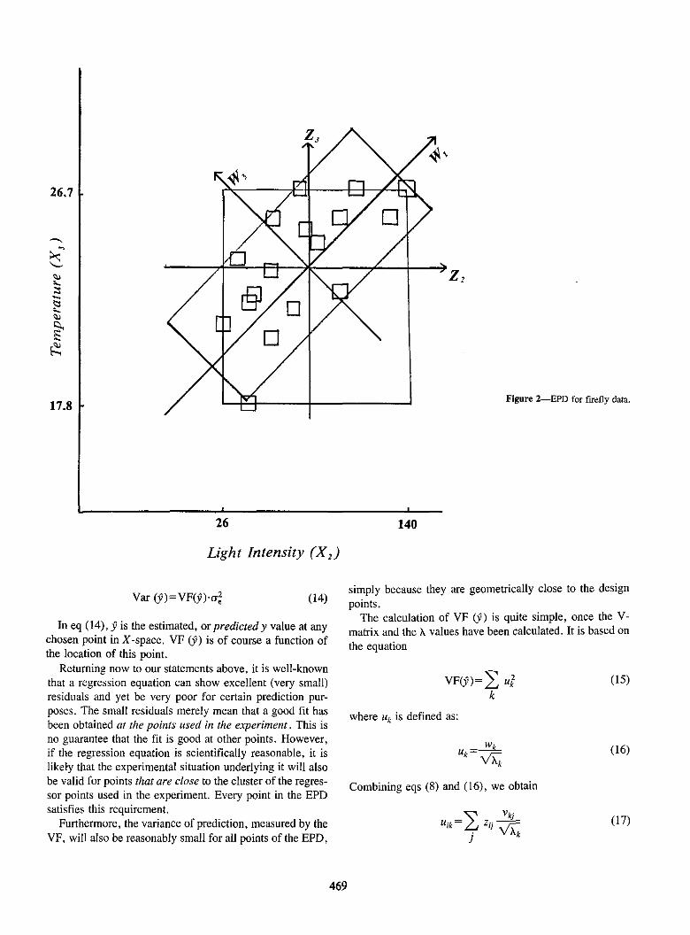
Z 2

Figure 2-EPD for firefly data.

-.1

140

Var (U) VF(i) .a 2 (14)

In eq (14), 9 is the estimated, or predicted y value at anychosen point in X-space. VF (v) is of course a function ofthe location of this point.

Returning now to our statements above, it is well-knownthat a regression equation can show excellent (very small)residuals and yet be very poor for certain prediction pur-poses. The small residuals merely mean that a good fit hasbeen obtained at the points used in the experiment. This isno guarantee that the fit is good at other points. However,if the regression equation is scientifically reasonable, it islikely that the experimental situation underlying it will alsobe valid for points that are close to the cluster of the regres-sor points used in the experiment. Every point in the EPDsatisfies this requirement.

Furthermore, the variance of prediction, measured by theVF, will also be reasonably small for all points of the EPD,

simply because they are geometrically close to the design

points.The calculation of VF (3) is quite simple, once the V-

matrix and the X values have been calculated. It is based onthe equation

(15)VFUf)=Z uk

k

where Uk is defined as:

Uk=c (16)

Combining eqs (8) and (16), we obtain

(17)Uik jE Zij V

469

26.7

it

9

17.8

26

Light Intensity (X2)

and hence:

(2 ZiJ",)

VFt-v)= A. (18)

Figure 3 shows the VF values at the vertices of the orig-inal sample domain and of the EPD. Interpreting these re-sults, we see that the collinearity of our data is reflected inthe rejection of an appreciable portion of the sample domainfor purposes of safe prediction. This does not mean thatprediction outside the EPD is impossible, or unacceptable.It merely means that such prediction cannot be justified onthe basis of the data alone. Of course, the risk of predictingoutside the EPD increases with the distance from the EPD.It will generally be reasonably safe to use the regressionequation even outside the EPD, as long as the point forwhich prediction is made is reasonably close to the bordersof the EPD. Using eq (18), the VF for any contemplatedprediction point is readily calculated and can serve as a basisfor decision.

Second Example:Calibration for Protein Determination

The instructive and intuitively satisfying graphical dis-play of the EPD becomes impossible when the number ofregressors, including the independent term, exceeds 3. Wemust then replace the graphical procedure by an analytical

d

C

Ib

one, as will now be shown in the treatment of our secondexample.

The data were presented by Fearn [3], in a discussion ofRidge Regression. They represent the linear regression ofpercent protein, in ground wheat samples, on near-infraredreflectance at six different wavelengths.

For reasons of simplicity in presentation, we include hereonly three of the six wavelengths, a change that has a rathersmall effect on the final outcome of the analysis: it turns outthat the regression equation based on these 3 wavelengths isvery nearly as precise as that based on 6 wavelengths.

The data, displayed in table 5, are a very good exampleof the use of regression equations: the regression equation isindeed to be used as a "calibration curve" for the analysis ofprotein, using the rapid spectrometry instead of the far moretime-consuming Kjeldahl nitrogen determination. Our datahave an N value of 24, and p (including the independentterm) is 4.

Table 6 exhibits the correlation matrix of the 24 designpoints. It is very apparent that the x values at all threewavelengths are highly correlated with each other, thus indi-cating a high degree of collinearity. At a first glance onewould be very skeptical about such a set of data, and suspectthat the X matrix shows such a high degree of redundancyas to make the regression useless for prediction purposes.Fearn explains that the correlations are more a reflection ofparticle size variability than of protein content. Our analysiswill confirm that, properly interpreted, the data lead to avery satisfactory calibration procedure.

We will find it useful to introduce a slightly different Ztransformation, which we call the Range-Midrange Trans-formation.

Sample Domain

VertexABCD

EPD

Vertexabcd

VF.39

1.71.69.30

Figure 3-VF at vertices of sampledomain and of EPD.

VF.41.41.41

.40

470

a

Table 5. Protein Calibration Data(')

ReflectanceX'2 X3

246 374236 386240 359236 352243 366273 404242 370238 370258 393264 384243 367233 365288 415293 421324 448271 407360 484274 406260 385269 389242 366285 410255 376276 396

% ProteinX4 Y

386 9.23383 8.01353 10.95340 11.67371 10.41433 9.51377 8.67353 7.75377 8.05398 11.39378 9.95365 8.25443 10.57450 10.23467 11.87451 8.09524 12.55407 8.38374 9.64391 11.35353 9.70445 10.75383 10.75404 11.47

Table 6. Protein calibration data-correlation matrix of x, through x4 .

I 0 0 01 .9843 .9337

i .9545l

The Range-Midrange Transformation

The Range-Midrange Transformation (RMT) is definedas follows:

Forj=l: zl=1 (19a)

EPD for the Protein DataThe EPD resulting from the Singular Value Decomposi-

tion based on the Range-Midrange Transformaton will notbe he same as the EPD we would have obtained using theCorrelation Scale Transformation, but we will see that thosefeatures of the EPD that are of importance for us, in estab-lishing the limitations of the regression equation, are practi-cally unaffected.

Table 7 shows the C and R values for the four regressorsand table 8 exhibits the V matrix and the X values obtainedfrom the Singular Value Decomposition. The latter, it maybe recalled, simply expresses the rotation of the Z coordinatesystem to the W system.

For each wk coordinate, there are 24 values, correspond-ing to the 24 regressor points.

Table 9 shows the smallest and the largest Wk value, foreach of the four k.

According to table 9, we must have, in the EPD:

(20)

with similar statements for w 2, W3, and w4. Applying now eq

Table 7. Protein calibration data-parameters for Z transformation(RMT).

j C R

1l0 1

2 296.5 63.53 418.0 66.04 432.0 92.0

Table 8. Protein calibration data-V matrix and X values (RMT).

k 1 2 3 4 X

X -. 6665 .4845 .4217 .3784 43.78102 .7365 .3299 .3797 .4523 8.37823 -. 1096 -. 5491 -. 2509 .7896 .37584 -. 0332 -. 5958 .7843 -. 1698 .06624

Forj>l: zj= iR i

but now C1 is defined as the midrange of the N values of xand Rj is one-half the range of these values. With thesedefinitions, it is clear that the smallest z-value, for anyregressor, is (-1) and the largest z-value is (+1). It isbecause of this - I to + I scale that this transformation wasintroduced. The benefits of this scale will become apparentin the following section.

Table 9. Protein calibration data-limits defining the EPD.

Coordinate(k) Smallest w Largest w

1 -1.9282 .61812 -. 4097 1.89893 -. 1669 .31584 -. 0801 .1324

471

Point

10

2345678910I11121314l5161718192021222324

(19b)

-1.9282�_wl_�.6181

(8), this double inequality can be written:

-1.9282C-.6665 zl+.4845 Z2+.4217 z3+.3784 z4

-3.6181

Since z, is constant and = I, this double inequality be-comes:

-1.2617' 4845 z2+.4217 Z3+.3784 z4t 1.2846 . (21a)

With the RMT, the value of any zk is, for any k > 1, between(-1) and (+ 1). Thus the expression in the middle has, forall design points, a value between -1.2846 and 1.2846,where 1.2846 is the sum of the absolute values of the threecoefficients. Therefore, the double inequality expressed byeq (21a) holds, essentially, for every point in the originalsample domain. Thus, wl, the first coordinate of the EPD,which represents its largest dimension, imposes essentiallyno restrictions on the sample domain.

Doing the same calculations for the three otherw-coordinates (see table 9), we obtain, respectively:

-I . 1462 .3299 Z2+.3797 Z3+.4523 Z4C 1 11619 (21b)

-0.568S -. 5491 z-.2509 Z3+.7896 z4- .4254 (21c)

-.0469 -. 5958 Z2+.7843 z3-.1698 z4s .1656. (21d)

We see that w2 too, imposes only very light restrictions onthe sample domain. On the other hand, W3 and W4 do implylimitations that eliminate appreciable portions of the sampledomain from the EPD.

We could readily convert eqs (21c) and (21d) to x coordi-nates by means of table 7 and eqs (19a) and (19b), but thez-coordinates, using the Range-Midrange Transformation,are more readily interpreted in terms of the severity ofcollinearity than the x-coordinates.

Thus, the sum of the absolute values of the coefficients inthe middle terms of (21c) and (21d) are 1.5896 and 1.5499,respectively. Points for which these linear combinationstake the valves ± 1.5896 and ± 1.5499 exist in the originalsample domain. The EPD, on the other hand, limits thesefunctions to intervals with much narrower limits.

Effect of Typeof Z Transformation

We have used two different Z transformations, the Corre-lation Scale, and the Range-Midrange. It is proper to askhow our results would have been affected in the ProteinCalibration Data, had we used Correlation Scale, instead ofthe Range-Midrange Transformation. We show the com-

Table 10. Protein calibration data-effect of Z transfornation. 1

w coordinate Z Transf. Inequalities

I CST -3.034 1.021 2+21.061 2,3+4•3.082RMT -3.334 1.280 z2+1.114 z3+z4•3.395

2 CSTRMT -2.534S•729 :z+.840 z3+z4•2.569

3 CST -. 075•-.686 z2-.321 z3+z4 .535RMT -. 072•-.695 z2-.318 z3+z4•.539

4 CST -. 278•-3.531 22+4.640 Z3-Z4• 980RMT -. 276s-3.509 z2+4.619 z3-,-4.975

'All inequalities are expressed in RMT z coordinates.

parison in table 10. Let us recall that with the CST, one ofthe w coordinates yields a X-value of unity, and a constantw value for all points. Therefore, we obtain for CST, onlythree sets of inequalities, as compared to the four sets forRMT. To allow the comparison between the two transfor-mation to be made, we have multiplied eqs (21a) through(2 Id) by positive constants, so as to make the coefficient ofz4 equal to ± 1. The same was done for the correspondinginequalities obtained by the Correlation Scale Transforma-tion.

Of course, since the z coordinates are different for the twotransformations, the inequalities for the CST, expressed inthe CST z-units, had to be converted to RMT z-units, for ameaningful comparison. As can be seen from table 10, thetwo smallest dimensions of the EPD are practically the samefor the two transformations. Thus, even though the methodof principal components is not invariant with respect tolinear transformations of scale, our analysis leads, in thiscase, to very similar results for the small dimensions of theEPD. We believe that this is generally true for all situationsin which collinearity is noticeable, i.e., for all situations inwhich the EPD eliminates considerable portions of the orig-inal sample domain. For situations in which this does notapply, i.e., totally non-collinear cases, the inequalities donot matter, since they impose no restrictions on the sampledomain.

It is interesting to contrast the remarkable similarity be-tween the inequalities for W3 and w4 for the two transforma-tions in table 10, with the behavior of a commonly advo-cated measure of collinearity (Belsley, Kuh, and Welsch[4], the condition-number.

The SVD resulting from the CST yields the followingeigenvalues: 2.9151, 1.0000, .07176, .01312. The condi-tion number is defined as the ratio of the largest to thesmallest eigenvalue. In this case:

condition number=2.9151/.01312=222.2

On the other hand, the SVD resulting from the RMT on thesame data yields the eigenvalues: 43.7810, 8.3782, .37575,.066244. This time we have:

472

condition number=43.7810/.066244=660.9

Thus the condition number varies considerably when thedata are subjected to different standardizing transforma-tions. It is not clear what useful information can be derived

from the condition number.By contrast, the treatment of collinearity we advocate has

a useful and readily understood interpretation: the EPD is

that part of the X space in which, and near which, prediction

is safe. It also indicates what portions of the original sample

domain are inappropriate for prediction on the basis of thegiven data alone. It fulfills this function in a way which ispractically invariant with respect to intermediate transfor-mations of scale. We use the qualifier "intenmediate" be-

cause collinearity has meaning only in terms of a given

original coordinate system (the X system). This system,which determines the original sample domain, must be con-

sidered fixed. On the other hand, transformations of this

system prior to calculating the EPD can be defined in differ-

ent ways without affecting the practical inferences drawn

from the data on the basis of the final EPD derived form the

standardizing transformation.

Cross-Validation

We can take advantage of the availability of a second set

of protein calibration data, also given in Fearn [3]; to verifythe correctness of our approach. Fearn lists 26 additionalpoints for which the reflectance measurements, as well as

the Kjeldahl nitrogen determination, were made. We ap-

plied the Z transformation obtained above (RMT on first setof 24 points) to each of these 26 points, and noted every

point for which at least one of the four sets of inequalities(21a) through (21d) failed to be satisfied. We found 14 such

points. This means that 14 "future points" obtained underthe same test conditions were outside the EPD establishedon the basis of the original 24 points. However, as we

observed above, as long as the point is not far from the EPD,prediction at that point is likely to be valid. We tested"predictability" at these 14 points by calculating the VF

value for each of them, and by comparing the predictedprotein value with the measured one. The results are shown

in table 11. It is apparent that all VF are relatively small,

indicating that even though these 14 points are outside the

EPD calculated from the original set, they are not far fromthat EPD. This is confirmed by the good agreement between

the observed and predicted values. The standard deviationof fit for the original set of 24 points was 0.23; the standard

deviation for a single measurement derived from the 14

differences in table 11 is 0.30.

Expansion Terms

Quite frequently, a regression equation contains x vari-ables that are non-linear functions of one or more of the

Table 11. Protein calibration data-cross-validation of analysis.

% ProteinPointl Observed Predicted VF

1 8.66 9.53 .2814 11.77 11.97 .4166 10.46 10.96 .1939 12.03 11.47 .212

10 9.43 9.54 .76211 8.66 8.15 .45412 14.44 13.99 .88114 10.41 10.17 .46816 11.69 11.24 .472

17 12.19 11.83 .39018 11.59 11.39 .31420 8.60 8.39 .20122 9.34 8.93 .15126 10.89 10.94 .741

rPoint in additional set (Fearn [3]) with its number designation in that set.

other x variables, such as x2, x2 x3 , etc. Polynomial regres-

sions are necessarily of this type. Since the x variables are

non-stochastic in the usual regression models, the least

squares solution for the regression equation is not affectedby the presence of such "expansion terms." On the other

hand, collinearity can be introduced, or removed, or modi-fied by them.

In our treatment the expansion terms cause no additionalproblems. Consider for example, the regression

(22)YI3tXl+p 2 X2+±3X2+E

with xl 31.

Here we have p = 3. Using RMT, followed by a singular

value decomposition, we obtain an EPD of three dimen-

sions, leading to the inequalities.

A1 •5v5B 1, A2 5w2 5B2 , A 3 •w 3•B 3 . (23)

Expressing the w as functions of the z, this leads to three

double inequalities governing the z, of the form

A,'-f 1 (z)•Bl, A2 •f 2(z)•B 2, A3 •f 3(z)5B 3 , (23)

2Now, since x3=x 2 , we have

X3 -C3 X22-C3 (R2Z2+C2 )2 -C3

Z3 R3 R3 R3

Hence:

CZi-C 3 2 C2 R2 R2 ,223= R3 2 R (24)

Because of this relation the functions fs(z),f2(z),f3(z) be-come functions of zl, Z2 (and Z2) only. Using this fact, we

473

interpret the three sets of inequalities (23) exactly as wehave interpreted eqs (21a) through (21d) by determiningwhich of these inequalities, if any, impose restrictions onthe use of the original sample domain.

To illustrate this procedure, consider the small set ofartificial data shown in table 12, for which the model isgiven at the bottom of the table. The term X3=x2 introducesa high correlation between x2 and X 3 and consequently alsoconsiderable collinearity.

The inequalities characterizing the EPD based on aRange-Midrange Transformation and converted to the z-scales, are shown in table 13. Applying eq (24) to expressz3 in terms of z2, the three double-inequalities become:

for wj:-.8 4 3 !5I.12 8 4 22+±2853 z2•1.4137for w2 :-.69285.8 5 4 1 Z2 +.1612 2.:1.0i53for W3 : .00775.0003 22+.3218 z224 .3221.

It is readily verified that of these six inequalities, all butone are satisfied for all 2z values between - I and + 1. Thelast one, involving the left side of the third set, is satisfiedfor all 22 values except for the interval: -. 15625.5 155.This corresponds to an x, interval between 2.1 and 2.8, orbetween the design points x,=2. 1 and x2 =3.6 (see table12). The interpretation of this finding is that while ail designpoints are of course inside the EPD, a small portion of thecurve x22 versus x2 falls slightly outside the EPD. This is ofno practical significance since the VF for these points, eventhough they are outside the EPD, does not exceed 0.58. Bycomparison, the smallest VF value along the curve, for therange xc,.2 to x2=4,7, is of the order of 0.26. Thus we seethat the serious collinearity in this data set is merely aconsequence of the presence of the expansion term x3=x2.

Table 12. An anificia' quadratic examplel.

Point y2 r3 P

1 .2 .04 28.32 .4 .16 27.53 1 1.00 25.64 2.1 4.41 28.75 3.6 12.96 46.46 4.7 22.09 69.8

'N = P3LL+PX2+,x23i3+: f3=30, R2=8, 1,=3.5. c,=0.2 xa~l.Nale Tha 3 x

Table 13. Quadratic examrple-inequalities for EPD.

r-coordinate Inequalities

w, -1.12815-.5070 z2+.6214 z3 •1.1284Wa -. 8541•.5029 z2+.3 511 z3 •. 85 4 1w3 -. 3141s-.7005 z2 +.7008 z3 5.0003

Any point in X space, in order to be acceptable, must lie onthe curve x 3=x22. An X3 with any other value is obviously notvalid and our analysis of the data, through the EPD, callsattention to this fact: in the direction of w3, the width of theEPD is only .31 as compared with widths of 2.26 and 1.71for w, and w,.

Discussion

The common mathematical definition of collinearity isthe existence of at least one linear relation between the xt's,of the form

E cjXj = OJ. j=I top (25)

where the cj are not all zero, and such that eq (25) holds withthe same cj values, for all i. This defines what we shall call"exact collinearity. " Geometrically, it means that all designpoints lie in an hyperplane of the x-space, going through theorigin of the coordinate system. Equation (25) also impliesthat the matrix X'X is singular, and consequently that theestimates of the 1 coefficients are not uniquely defined.

Exact collinearity seldom occurs in real experimental sit-uations; indeed, if theX matrix is notthe result of a designedexperiment, it is highly improbable that a relation such as eq

(25) would hold exactly. If, on the other hand, the experi-ment is designed, care would generally have been taken toavoid a situation of exact coilinearity.

While exact collinearity is practically of little concern,near-collinearity is a frequent occurrence in real-life data.This occurs when an equation such as (25) is "approx-imately" true for all i. Many attempts have been made todefine more closely the concept of near-collinearity, butwhile these endeavors have led to a number of proposals formeasuring collinearity, they are of little practical use to theexperimenter confronted with the task of interpreting hisdata.

It is not our intention to discuss here the pros and cons ofthe various attempts made by a number of authors to"remedy" a near-collinear situation. The best-known ofthese remedial procedures is Ridge Regression. We merelyrepeat what we have said in the body of the paper: anyattempt to remedy collinearity must necessarily be based onadditional assumptions, unless it consists of making addi-tional measurements, The latter alternative is of course log-ical and valid, but the making of assumptions inventedspecifically for the purpose of removing collinearity doesnot appear to us to be a recommendable policy in dataanalysis.

One easily recognizable condition leading to collinearityis the existence of at least one high correlation coefficientamong the non-diagonal elements of the correlation matrix

474

of the x's. This has given rise to the concept of the VarianceInflation Factor (VIF). The VIF for 13> is defined (Draper

and Smith [5]), as:

VIF(0)= I1 (26)

where R1 is the multiple correlation coefficient of xj on all

other regressors. If d represents a residual in this regression,the usual formula for Rj is given by

Rj2= I _ Ed 2 (27)E(XjXj)2

Now, Snee and Marquardt (Belsley [6], "comments") make,implicitly, a distinction between the two "models":

Y=3 1 xI+ 32 x2 + +R3pxp+E (28a)

with xsl 1, and

Y - =,02(X2-32)+ " +, p(Xp -Rp)+E (28b)

where (28b) is called the "centered" model. For (28b), Snee

and Marquardt use eq. (27), but for (28a) they appear to use

the definition:

R l E21 _ d2 (29)

Equation 29, in which the denominator of the last term is not

centered, is not explicitly given by Snee and Marquardt, but

is implied by their statement:"If the domain of prediction includes the full

range from the natural origin through the range of

the data, then collinearity diagnostics should notbe mean-centered," and confirmed by the VIFvalues given in their table 1. In this table, "no

centering" results in VIF values of 200,000 and400,000, while the VIF for the "centered" data are

unity. The quoted statement occurs in a section

entitled "Model building must consider the in-tended or implied domain of prediction." The

basic idea underlying the section in question is

that the analysis of the data, based on the"collinearity diagnostics" (specifically: the VIF

values), is goverened by the location of the points

were one wishes to make predictions and, morespecifically, on whether the origin (xl=I,

x2=x3 .. =0) is such a point. The VIF valueswhich, according to Snee and Marquardt's formu-

las, depend heavily on whether or not this originis included, will then indicate the quality of the

predicted values.A more reasonable approach, and one more consistent with

the procedures commonly used by scientists, is to limit

prediction to the vicinity of where one made the measure-

ments, unless additional information is available that justi-fies extrapolation of the regression equation to more distantpoints of the samples space. The vicinity of the measuredpoints is determined by the EPD which, in the case ofcollinearity, may be considerably smaller than the sample

domain. In this view, it is the location of the design points,

rather than that of the intended points of prediction, thatdetermines predictability. The latter is measured, not by

VIF values, but rather by the more concrete VF values, for

any desired point of prediction.The view advocated by Snee and Marquardt sometimes

results in an enormous difference in the VIF values between

the centered and non-centered forms. Equation 29 serves no

useful purpose and is, in fact, unjustified and misleading. It

is unjustified because it not only includes the origin (xi = 1,

xk =0 for k>l) in the correlation and VIF calculations, butmoreover, gives this point infinite weight in these calcula-

tons. Yet, no measurement was made at that point. Equation

29 is also misleading because it leads to very large VIF

values for some non-centered regressions, implying thatsevere "ill-conditioning" exists, even when the X matrix is

except for some trivial coding, completely orthogonal (cf.

[6]).The ill-conditioning exists only in terms of the large VIF

value. It is an artifact arising from the desire to make the two

forms of the regression equation into two distinct "models".The two forms, eqs 28a and 28b lead to identical esti-

mates for the 13>, including PI, and for their standard errors.

They also lead to identical values and variances for an esti-

mated (predicted) v, at any point of the X space. There

seems to be no valid reason for the two distinct equations for

the VIF. They only lead to the false impression that center-

ing can reduce or even remove collinearity.Our viewpoint in this paper is that the usefulness of a

regression equation lies in its abilty to "predict" y for inter-

esting combinations of the x's. We also take the position

that inferences from the data alone should be confined to x

points that are in the general geometric vicinity of the cluster

of design points. An inference for points that are well out-

side this domain (i.e., outside a suitably defined EPD) is, in

the absence of additional information, only a tentative con-

clusion, and not a valid scientific inference. Such conclu-

sions may however, be very useful, provided their tentative

character is recognized, and provided they are subsequently

subjected to further experimental verification.Daniel and Wood [7] discuss briefly the relation between

the variance of 9 and the location of the point at which the

prediction is made. However, their discussion is in the con-

475

text of selecting the best subset of regressors from amongthe entire set of regressors, a subject different from the onedealt with in this paper.

Another publication that deals explicitly with predictabil-ity is a paper by Willan and Watts [8]. These authors definea "Region of Effective Predictability" (REPA) as that portionof the X space in which the variance of the predicted 5 doesnot exceed twice the variance of 5 predicted at the centroidof the X matrix. The volume of the region is then comparedwith that of a similarly defined REP, denoted REPO. Thelatter refers to a "fictitious orthogonal reference design" of"orthogonal data with the same N and the same rms valuesas the actual data." The ratio of the volume of REPA to thatof REPO is taken as "an overall measure of the loss ofpredictability volume due to collinearity".

This concept, apart from its artificial character, suffersfrom other shortcomings. Like so many other treatments, itattempts to provide a measure of collinearity. But the prac-titioner who is confronted with a collinearX matrix does notneed a measure of collinearity: he needs a way to use thedata for the purpose for which they were obtained. Further-more, this measure loses its meaning when expansion vari-ables are present. For example, for the artificial quadraticset of table 12, Willan and Watts' measure would indicatea high degree of collinearity which, while literally true, istotally misleading since the collinearity in no way reducesthe usefulness and predicting power of the regression equa-tion, as long as the meaning of the expansion term is takeninto account. But even in cases withoutexpansion terms, themeasure in question may be misleading. Thus when appliedto the protein calibration data of table 5, it may well lead theanalyst to give up on these data as a hopelessly highly-collinear set, whereas, as we have seen, there is nothingwrong with this set and it can indeed be used very effec-tively for the calibration of a method for protein determina-tion based on reflectance measurements.

Finally, a few words about estimating the ,,-coefficientsconsidered as rates of change of y with changes in theindividual xp. As pointed out by Box [9], this is generallynot a desirable use of regression equations. If, however, it

is the major purpose of a-particular experiment, then thisexperiment should be designed accordingly, which means:essentially with an orthogonal X matrix. A collinear X ma-trix leads to the ability to estimate certain linear combina-tions of the O's much better than the Os's themselves. Theexperimenter can calculate the VF values, not only for anypoint of X space, but also for any 1) or combination of Pl's,and he can do this without making a single measurement,i.e., in the planning stages of the experiment. If the exper-imenter does not take advantage of this opportunity, he maybe in for considerable disappointment, after having spenttime, money, and effort on inadequate experimentation. Webelieve that he advocacy of remedial techniques, such asRidge Regression for collinear data is unwise. One of themost important tasks of a data analyst is to detect, and to callattention to, limitations in the use and interpretation of thedata.

References

[X] Buck, J.B.. Studies on the Firefly, Part 1: The Effects of Light andOther Aspects on Flashing in Photinus Pyralic, with Special Ref-erence to Periodicity and Diumal Rhythm, Physiological Zool-ogy, 10, 45-58 (1937).

[2] Mandel. J., Use of the Singular Value Decomposition in RegressionAnalysis, The American Statistician, 36, 15-24 (1982).

[3] Fearn, T., A Misuse of Ridge Regression in the Calibration of a NearInfrared Reflectance Instrunment, Applied Statistics, 32, 73-79(1983).

[4] Belsley. D.A., E. Knu, and R.-. Welsh, Regression Diagnostics:Identifying Influential Obserwations and Sources of Collinearity,Wiley, NY (1980).

[5] Draper, N.R. and H. Smith, Applied Regression Analysis, Wiley,2nd Edition, NY (1981).

[6] Belsley, DA., Demeaning Conditioning Diagnostics Through Cen-tering, The American Statistician, 38, 73-77, and "Comnrents",78-93 (1984).

[7] Daniel, C.. and F.S. Wood, Fining Equations to Data, Wiley, 2ndEdition, NY (1980).

[8] Willan, A.R. and D.G. WaVts, Meaningful Multicollinearity Mea-sums, Technometrics, 20, 407-12 (1978).

[9] Box, G.E.P., Use and Abuse of Regression, Technometrics 8 625-29(1966).

476

DISCUSSIONof the John Mandel paper, The RegressionAnalysis of Collinear Data

R. W. GerlachMonsanto Agricultural Products Co.

I fully agree with Mandel in that one's model can (usu-

ally) only be assigned a degree of validity in the region

spanned by the data used to generate the model. Though the

range for all variables may be quite large, collinearity effec-

tively restricts the model to a particular subregion. One

should be aware of these restrictions so as not to misapply

the model to those regions not represented by the data. I

want to point out the need to carry out an additional initial

operation; one should always examine the dataset for out-

liers. Otherwise the suggestion for using the largest and

smallest values on each principal coordinate to examine the

constraints may lead to overstating the region for a valid

calibration. In fact, this could happen anyway if the shape

formed by the data vectors was peculiar, perhaps occupying

two disjoint regions for instance.Additional constraints are frequently available to the ana-

lytical chemist. Minimum and maximum values along the

original variables as well as conditions upon functions of

these variables are frequently encountered. The location of

the effective predictive domain within this potentially al-

lowed domain could also be useful. A comparison might

lead the researcher to conclude that more effort should be

spent gathering additional data so that the calibration equa-

tion was valid over the desired region.The variance factor (VF), resulting from the propagation

of errors through the transformations, is a good method for

observing how well characterized the model is at any loca-

tion. Though principal components regression has been in

the literature of analytical chemistry for some time [1,2]' a

paper dealing with the region of applicability for the model

has only recently been published [3]. In this case the authors

used as their criteria the expected mean square error. Hope-

fully, the propagation of error in this and related techniques

will become more commonplace in analytical chemistry.

I think that the comparison of the measures advocated in

this paper to the condition number is somewhat misdirected.

The condition number can be used to provide a measure of

how sensitive a model could be to variations in the data

matrix. However, it would certainly not be appropriate to

consider a condition number for the complete data matrix if

one is dealing with only a subset of its dimensions in the

principal component regression. The condition number

tFigures in brackets indicate literature references.

assists one in interpreting the sensitivity of the model given

all the original variables (or any orthogonal transformation).

The condition number for the rotated coordinate system ofthe principal coordinates will be the same as for the original

coordinate system. In the original coordinate system a large

condition number signaled that the regression coefficients

were not all well known. In the rotated eigenvector coordi-

nate system this same condition number reflects the fact that

coefficients for the eigenvectors with small eigenvalues will

not be estimated accurately. However, since only the eigen-

vectors with significant eigenvalues will be considered in

the principal component regression, the condition number

for the entire matrix is not an appropriate parameter to

consider. In fact, the only thing we can say is that one

expects large condition numbers every time a principal com-

ponent regression is the method of choice.It should also be pointed out that other aspects of

collinearity are frequently encountered by analytical

chemists. While this paper deals with collinearity as it af-

fects the region for applicability of the model in terms of

predictability, it doesn't address questions as to the reliabil-

ity of the model coefficients. Also, instead of generating a

calibration or predictive equation, one might wish to evalu-

ate possible models in which the independent factors behave

somewhat similarly. What limitations are placed on the re-

sults of the traditional regression analysis? I want to mention

that statisticians have already developed several appropriate

techniques [4], such as methods to estimate confidence re-

gions and the effective sample size. Hopefully, these and

other measures to test the validity of the proposed model

will be more widely used.The propagation of errors through a constrained corre-

lated regression would also be an appropriate technique for

investigating the significance of the terms in a proposed

model. As mentioned above, often there are known con-

straints, yet this information is commonly overlooked. A

recent comparison of multivariate techniques applied to

source apportionment of aerosols in which collinearity was

an important factor showed that the known constraints were

mostly ignored [5]. Mathematical techniques which deal

with these extra conditions [6], though more complex nu-

merically, should be investigated for their potential benefits

to areas of analytical chemistry and brought into more com-

mon use.

477

References

[I] Bos. M.. and G. Jasink, The Learning Machine in QuantitativeChemical Analysis. Analwica C/inica Acta 103. pp 151-165(1978).

121 Martens. H.. Factor Analysis of Chemical Mixtures, Analywica C/him-ica Acta 112. pp 423-442 (1979).

(31 Fredericks, P. M.- Lee, J. B.; Osborn. P. R., and D. A. J. Swinkels,Materials Characterization Using Factor Analysis of FT-IR Spec-tra. Part 2: Mathematical and Statistical Considerations, AppliedSpectroscopy 39, pp 311-316 (1985).

414 Willan. A. R., and D. G. Watts. Meaningful Multicollinearity Mea-sures, Techncoetrics 20, pp. 407-412 (1978).

151 Currie, L. A.; Gerlach, R. W., and C. W. Lewis, et al, Interlabora-tory Comparison of Source Apportionment Procedures: Resultsfor Simulated Data Sets. Atmnosp/heric Environmelrnt 18, pp 1517-1537 (1984).

161 Rust. B. W., and W. R. Butrus. Mathematical Programming and theNumerical Solution of Linear Equations, Elsevier (1972).

478

journal of Research of the National Bureau of StandardsVolume 90, Number 6, November-December, 1985

Optimization

Stanley N. DemingUniversity of Houston-University Park, Houston, TX 77004

Accepted: July 1, 1985

Most research and development projects require the optimization of a system response as a function of severalexperimental factors. Familiar chemical examples are the maximization of product yield as a function of reaction timeand temperature; the maximization of analytical sensitivity of a wet chemical method as a function of reactantconcentration, pH, and detector wavelength; and the minimization of undesirable impurities in a pharamaceuticalpreparation as a function of numerous process variables. The "classical" approach to research and development involvesanswering the following three questions in sequence:

I) What are the important factors? (Screening)2) In what way do these important factors affect the system? (Modeling)3) What are the optimum levels of the important factors?

As R. M. Driver has pointed out, when the goal of research and development is optimization, an alternative strategyis often more efficient:

I) What is the optimum combination of all factor levels? (Optimization)2) In what way do these factors affect the system? (Modeling in the region of the optimum)3) What are the important factors?

The key to this alternative approach is the use of an efficient experimental design strategy that cam optimize a relativelylarge number of factors in a small number of experiments. For many chemical systems involving continuously variablefactors, the sequential simplex method has been found to be a highly efficient experimental design strategy that givesimproved response after only a few experiments. It does not involve detailed mathematical or statistical analysis ofexperimental results. Sequential simplex optimization is an alternative evolutionary operation (EVOP) technique that isnot based on traditional factorial designs. It can be used to optimize several factors (not just one or two) in a single study.Some research and development projects exhibit multiple optima. A familiar analytical chenical example is columnchromatography which often possesses several sets of locally optimal conditions. EVOP strategies such as the sequentialsimplex method will operate well in the region of one of these local optima, but they are generally incapable of findingthe global or overall optimum. In such situations, the "classical" approach cam be used to estimate the general regionof the global optimum, after which EVOP methods can be used to "fine tune" the system. For example, in chromatog-raphy the Laub and Purnell "window diagram" technique cam often be applied to discover the general region of the globaloptimum, after which the sequential simplex method cam be used to "fine tune" the system, if necessary. The theoryof these techniques and applications to real situations will be discussed.

Key words: optimization; screening: simplex.

1 Introduction 1 ) re-establishing acceptable product yield as a function ofreaction time and reaction temperature after a design

Most research and development projects require the opti- change in a chemical process;mization of a system response (dependent variable) as a 2) maximizing the analytical sensitivity of a wet chemicalfunction of several experimental factors (independent vari- method as a function of reactant concentration, pH, andables). Familiar chemical examples are: detector wavelength;

3) tuning-up a nuclear magnetic resonance spectrometer byAbout the Author: Stanley N. Deming is with the De- adjusting eleven highly interacting shim coil controls to

partment of Chemistry at the University of Houston- produce optimum peak shape.University Park. 4) finding a combination of values for eluent variables that

479

will give adequate separation in high performance liquidchromatography.

Although "optimization" is often taken literally to meanmaking something "as perfect, effective, or functional aspossible" [1]l, in chemical practice it usually means makingsomething "acceptable" or "adequate," as in examples oneand four above. Optimization in chemistry usually involvesadjusting a system until it is brought to some desiredthreshold of performance.

The dual purposes of this short paper are to discuss sev-eral strategies for the optimization of chemical systems andto discuss strengths, weaknesses, and appropriate settingsfor each approach. The intent of these comments is not tosuggest rigid guidelines for the proper uses of optimizationmethods, but rather to stimulate discussion directed towarda better understanding of how these methods can be used inpractice.

2. Classical Experimental Designs

The "classical" approach to optimization in research anddevelopment involves answering the following three ques-tions in sequence:

1) What are the important factors? (SCREENING)2) In what way do these important factors affect the system?

(MODELING)3) What are the optimum levels of the important factors?

(OPTIMIZATION)

Classical experimental designs (e.g., fractional factorialdesigns and central-composite designs [2,3]) can be used toscreen factors and to acquire data for modeling the systemas a function of the most important variables. The resultingmodel can then be used to predict the treatment combination(experimental conditions) giving the optimum response [4-6]. The statistical literature is rich in examples showing howstatistically designed experiments have been used in thisway to solve significant chemical problems (e.g., [7]).A. Modeling

The critical part of the classical approach is the secondstep, modeling. At the very least, a model that fits reason-ably well over a limited region of the factor space can beused to predict a direction to move to obtain improvedresponse (as in evolution operation, or EVOP [8]). A modelthat fits well over a larger region of factor space is, ofcourse, even more useful. However, if the (usually empiri-cal) model contains more than a few factors, then the num-ber of experiments required to fit the model will be imprac-tically large. For example, if a full second-order polynomialmodel containing k factors is used to model the system, thenumber of model parameters will be equal to (k + 1)(k +2)!

TFigures in brackets indicate literature references.

2; for five, six, seven, and eight factors the numbers ofmodel parameters are 21, 28, 36, and 45, respectively. Atleast this many experiments must be carried out to providedata for the estimation of the parameter values; typically,central composite designs are used which require 2k+3k+1experiments (plus three replicates to estimate "pure error")for a total of 46, 80, 146, and 276 experiments for five, six,seven, and eight factors, respectively.

Thus, a desire to avoid extraordinarly large numbers ofexperiments becomes a strong driving force for limiting(typically to only thee or four) the number of factors to beinvestigated by classical experimental designs. Hence, theneed for the initial screening of factors to choose only themost important ones.B. Screening

There are problems with screening experiments. For ex-ample, most screening experiments are based on first-ordermodels which assume no interactions. If interactions doexist, then factors which truly have a significant affect onthe system might not appear to be statistically significantand would be discarded by the screening process.

A second problem with screening experiments can occurif the effect of a factor depends upon its own level "selfinteraction"). If screening experiments are carried out in aregion where the response is "flat" with respect to the factorof interest (a stationary region), that factor will not appearto a be very significant when, in fact, at different levels ofthat factor, the effect on response might be considerable.

As a final example of difficulties in screening for signif-icant factors, the "wrong" statistical test is usually usedwhen screening factors for their significance. It is true thatif a factor is "significant at the 95% level of confidence,"then it is probably an important factor and should be retainedfor further investigation. However, if a factor is "not signif-icant at the 95% level of confidence," it does not mean thatit is an unimportant factor and can be neglected. It might,for example, be significant at the 94.73% level of confi-dence, not enough to exceed the common threshold of 95%confidence, but still highly significant nonetheless. Ideally,the question that should be asked while carrying out screen-ing experiments is not "which factors are significant at somehigh level of confidence," but rather, "which factors areinsignificant at some equally high level of confidence."Unfortunately, the type of experimentation required to an-swer this second question is extensive and expensive. Analternative approach is to increase the risk (alpha) of statingthat a factor is significant when in fact it is not, so that fewertruly significant factors are rejected [9].C. Comments on the use of classical experimental de-

sign for optimizationClassical experimental designs appear to have been suc-

cessful in the past for "optimizing" many existing chemicalsystems largely because these systems are usually run not atthe true optimum but rather are operated at some "threshold

480

of acceptability." A response surface view of this would bethat the system is being run at a point on the side of a hill;

not at the top of the hill, but far enough up on the side thatthe system gives acceptable performance. As long as the

response surface maintains its shape and position, and aslong as the factor levels are kept in statistical control, thesystem will perform acceptably.

However, if the response surface changes its shape or"'moves" slightly (as a result, for example, of scale buildupin heat exchangers, or different suppliers of feed stocks),then the previous set of factor levels might no longer pro-duce adequate performance from the system: the same set-point will now correspond to some slightly lower position on

a changed response surface. In situations like this, smallscreening experiments (such as saturated fractional factorialdesigns [2] or Plackett-Burmann designs [101 are not toomuch affected by factor interactions and are likely to givenearly true estimates of the first-order factor effects (e.g.,the effect of temperature, or the effect of increased amountsof feed stocks). Similarly, a first-order model offers a goodapproximation to the true shape of the response surface overa limited region. Thus, the application of screening experi-ments to choose the most significant factors is usually suc-cessful in this application. When these most significant fac-tors are used in a model of the system that is first-order withinteractions (fitted, say, to the results of a two-level factorialdesign), then the fitted model will usually suggest an appro-priate direction to move. Changing the factor levels in thisdirection will usually move "up" the hill to a point lyingabove the threshold of performance and once again achieveadequate ("optimum") response from the system.

3. Sequential Simplex Optimization

As R.M. Driver has pointed out [11], when the goal ofresearch and development is optimization, an alternativestrategy is often more efficient. This alternative strategyasks essentially the same questions as the classical approachto optimization, but it asks the questions in reverse order:

1) What is the optimum combination of all factor levels?

(OPTIMIZATION)2) in what way do these factors affect the system? (MOD-

ELING in the region of the optimum)3) What are the important factors? (SCREENING for ef-

fects in the region of the optimum)

The key to this alternative approach is the use of anefficient experimental design strategy that can optimize arelatively large number of factors in a small number ofexperiments. Once in the region of the optimum, classicalexperimental designs can be used to full advantage to modelthe system and determine factor importance in a limited

region of the total factor space.

A. ignoring Initial Screening Experiments and Avoid-ing Models

For many chemical systems involving continuously vari-able factors and relative short times for each experiment, the

sequential simplex method [12-38] has been found to be ahighly efficient experimental design strategy that gives im-proved response after only a few experiments. It is alogically-driven algorithm that does not involve detailedmathematical or statistical analysis of experimental results.Sequential simplex optimization is an alternative evolution-ary operation (EVOP) technique that is not based on tradi-tional factorial designs.

There are two reasons for the efficiency of the sequentialsimplex method. The first reason is the number of experi-ments required in the experimental design itself. A simplexis a geometric figure containing a number of vertexes equalto one more than the number of dimensions of the factorspace. Each vertex locates a treatment combination in factorspace. Thus, the number of experiments required for a sim-plex is k + I where, again, k is the number of factors. Thus,a five, six, seven, or eight factor system would require only6, 7, 8, or 9 experiments to define a simplex.

The second reason for the efficiency of the sequentialsimplex method is that it takes only one or two additionalexperiments to move the experimental design into an adja-cent region of factor space. This is independent of the num-ber of factors involved. When classical experimental de-signs are used in this type of "evolutionary operation" mode,a larger number of experiments (at least half of the factorcombinations in the pattern) is usually required to move theexperimental design into an adjacent region of factor space.

In our experience with the simplex, systems of up to 11factors can be brought into the region of the optimum in only15 or 20 experiments after the initial simplex has beenconstructed.B. Limitations

The simplex does have its limitations, however. The sys-tem must be in "statistical control" if the simplex is to beused-that is, the system should have only a small amountof purely experimental uncertainty ("pure error"), It is rec-ommended that after the initial simplex has been evaluatedand before the first simplex move is begun, the vertex givingthe worst response and the vertex giving the best responsebe repeated two more times each to evaluate the reproduci-bility of the system. If the reproducibility is good, then thesimplex will progress well; if the reproducibility is poor,then the simplex will tend to wander. In this latter case,steps should be taken to improve the purely experimentaluncertainty of the system; if this is not possible, then classi-cal experimental designs offer advantages because of theirnoise-reducing capabilities [39].

The system should not drift with time. However, changeswith time can often be detected and corrected for by runningperiodic experiments at a standard treatment combination.

481

The time of any one experiment must be relatively short.It has been suggested that the reason factorial experimentswere developed before the sequential simplex was becauseof the experimental environment, specifically the improve-ment of agricultural crop yields. In this context, factorial

experiments offer a great advantage in that several experi-ments can be carried out simultaneously and many resultscan be obtained after only one growing season. If the se-quential simplex were to be used to improve agriculturalproduction., only one move could be carried out each yearand it could take several decades to optimize production,

Finally, the simplex is most powerful for continuous("quantitative") variables. It can be used for discrete vari-

ables where there are several levels-perhaps at least five orsix-and the Levels can be logically ranked. It can not beused for unranked discrete ("qualitative") variables.

4. Systems Possessing Multiple Optima

Some research and development projects exhibit multipleoptima. A familiar analytical chemical example is columnchromatography which often possesses several sets of lo-cally optimal conditions [40]. The reason for the existenceof multiple optima is related to the phenomenon of changesin the order of elution with changing chromatographic con-ditions. EVOP strategies such as the sequential simplexmethod will operate well in the region of one of these localoptima, but they are generally incapable of finding theglobal or overall optimum [23]. In such situations, classicalfactorial-type experiments can be used to fit models whichin turn can be used to estimate the general region of theglobal optimum, after which EVOP methods can be used to"fine tune" the system. For example, in chromatography theLaub and Purnell "window diagram" technique [40] canoften be applied to discover the general region of the globaloptimum, after which the sequential simplex method can beused to "fine tune" the system, if necessary [41-491.

References

[1] Websner's New Collegiate Dietionary, G. & C. Merriam Company,Springfield. MA (1977), p. 806.

[2] Box, G.E.P.; Hunter, W.G. and J.. Hunter, Statisticsfor Experi-menters,' An Introduction to Design, Data Analysis, and ModelBuilding, Wiley, New York, NY (1978).

[3] Deming, S.N. and SL. Morgan, The Use of Linear Models andMatrix Least Squares in Clinical Chemistry, Cin. Chnem, 25, 840(1979).

[4] Box, G.E.P., and K.B Wilson, On the Experimentral Attainment ofOptimum ConditionsJ. Roy. Stat. Soc., Ser. B, 13, 1 (1951).

[51 Box, G.E.P., The Exploration and Exploitation of Response Sur-faces: Some General Considerations and Examplies, Biometrics,10, 16 (1954).

[6] Box, G.E.P., and P.V, Youle, The Exploration and Exploitation ofResponse Surfaces: An Example of the Link Between the Fitted

Surface and the Basic Mechanism of the System. Biometrics, 1l,287 (1955).

[7] Davies, O.L., Ed., Design and Analysis of Industrial Experiments,2nd ed., Hafner, New York, NY (1971).

[8] Box, G.E.P., and N. R. Draper, E'oludon Operation. A SlatisticalMethod for Process Improvement, Wiley, New York, NY (1969).

[9] Wilson, E.B., Jr., An Introduction to Scientific Research, McGraw-Hill, New York, NY (1952), p. 59.

(101 Ptackett, R.L., and Ji.P Barilama'he Design ofOptimnum Muttifac-tonal Experiments," Bionietrika, 33, 305 (1946).

[11] R.M. Driver, Chem. Brit. . 6, 154 (1970).

[121 Spendtey, W.; Hext, G.R., and F. R. Himsworth, Sequential Appli-cation of Simplex Designs in Optinization and Evolutionary Op-eration, Technomeetrics, 4, 441 (1962).

[13] Nelder, J.A., and R. Mead, A Simplex Method for Function Mini-

ndzation, Computer J.. 7, 308 (1965).[14] Derming, S.N., and S.L. Morgan, Simplex Optimization of Variables

in Analytical Chernisy, Anal. Chemt., 45, 278A (1973).[15] Deming, S.N. and P.G. King, Computers and Experimental Opti-

mization, ResearchlDevelopmenr, 25(5), 22 (1974).[16] King, P.C., Automated Development of Analytical Methods, Ph.D.

Dissertation, Emory University, Atlanta, GA (1974).[17] Morgan, S.L., and S.N. Derning, Simplex Optimization of Analyti-

cal Methods, Anal. Chenm., 46, 1170 (1974).(18) King, P.G., and S. N. Deming, UNIPLEX: Single-Factor Optimiza-

tion of Response in the Presence of Error, Anal. Chem., 46, 1476(I974).

(19] Yarhro, L.A., and S.N. Deming, Selection and Preprocessing ofFactors for Simplex Optimization, Anal. Chinm. Acta, 73, 391([974).

[20] King, P.G.; Denming, SN.. and S.L. Morgan, Difficulties in theApplication of Simplex Optimization to Analytical Chemistry,Anal. Lett., 8, 369 (1975).

[21] Parker, L.R., Jr., Morgan, S.L, and S.N. Deming, Simplex Opi-nization of Experinmental Factors in Atomic Absorption Spec-trometry, App. Spec-tosc., 29, 429 (1975).

[22] Dean, W.K.; Heald, K.J., and S.N. Deming, Simplex Optimizationof Reaction Yields, Science, 189, 805 (1975).

[23] Morgan, S.L., and SN. Dening, Optimization Strategies for theDevelopment of Gas-Liquid Chromatographic Methods, J. Chro-masogr., 112, 267 (1975).

[24] Olansky, A.S., and S.N. Deming, Optimization and Interpretation ofAbsorbance Response in the Determination of FormiAdehyde withChromotropic Acid, Anl. Chin. Acia, 83, 241 (1976).

[25] Deming, S.N., Morgan, S.L., and M.R. Willcott, Sequential Sim-plex Optimization, Amer. Lab., 8(10), 13 (1976).

[26] Turoff, M.L.H. and S .N. Deming, Optimization of the Extraction ofIron (II) from Water into Cyclohexane with Hexafluorcacetylace-tone and Tri-n-Butyl Phosphate," Telrato, 24, 567 (1977).

[27] Deming, S.N. and S.L. Morgan, Advances in the Application ofOptimization Methodology in Chemistry. Chapter I in B.R.Kowalski, Ed., Chemonretrics: Theory and Application, ACSSymposium Series 52, American Chemical Society, 1977, p. 1.

[28] Deeming,S.N., OptimzationofExpefimnentalPanmetersinChemicalAnalysis, Chapter 5 in J.R. DeVoe, Ed., Validation of the Mea-surenent Process, ACS Symposium Series 63, American Chemi-cat Society, 1977, p. 162.

[29] Olansky, A.S., Parker, L.R., Jr., Morgan, S.L., and S.N. Deming,Automated Development of Analytical Chemical Methods. TheDeterirnation of Serum Calciunm by the Cresolphthalein Corn-plexone Method, Anal. Chim. Acta, 95, 107 (1977).

[30] Deming, S.N. and L.R. Parker, Jr., A Review of Simplex Optimiza-tion in Analytical Chemistry, CRC Cri1. Rev. Anal. Chemn., 7,187 (1978).

482

[31] Deming, S.N., Optimization of Methods, Chapter 2 in R.F. Hirsch,Ed., Proceedings of the Eastern Analytical Symposium on Princi-ples of Experimentation and Data Analysis, Franklin InstitutePess, 1978, p. 31.

[32] Olansky, A.S. and S.N. Deming, Automated Development of a Ki-netic Method for the Continuous-Flow Determination of Crea-tinine, Clin. Chem., 24, 2115 (1978).

[33] Shavers, C.L., Parsons, M.L., and S.N. Deaming, Simplex Optimiza-tion of Chemical Systems, J. Chem. Educ., 56, 307 (1979).

[34] Deming, S.N., The Role of Optimization Strategies in the Develop-ment of Analytical Chemical Methods, American Laboratory,13(6), 42 (1981).

[35] Deming, S.N. and S.L. Morgan, Teaching the Fundamentals of Ex-perimental Design, Anal. Chim. Acta., 150, 183 (1983).

(36] Nickel, J.H. and S.N. Deming, Use of the Sequential Simplex Opti-mization Algorithm in Automsted Liquid Chromatographic Meth-ods Development, LC, 414 (1983).

[37] Golden, P.J. and S.N. Deming, Sequential Simplex Optimizationwith Laboratory Microcomputers, Laboratory Microcomputers,3(2), 44 (1984).

[38] Walters, F.H. and S.N. Deming, A Two-Factor Simplex Optimiza-tion of a Programmed Temperature Gas Chromatographic Separa-tion, Anal, Left., 17, 2197 (1984).

[39] Mendenhall, W. Introduction to Linear Models and the Design andAnalysis of Experiments, Duxbury, Belmont, CA (1968).

[40] Laub, R.J. and J.H. Purnell, J. Chromarogr, 112, 71 (1975).[41] Morgan, S.L. and S.N. Deming, Experimental Optimization of Chro-

matographic Systems, Sep. Purif Methods, 5, 330 (1976).[42] Deming, S.N. and M.L.H. Turoff, Optimization of Reverse-Phase

Liquid Chromatographic Separation of Weak Organic Acids,Anal. Chem., 50, 546 (1978).

[43] Price, W.P., Jr.; Edens, R., Hendrix, D.L., and S.N. Deming, Opti-mized Reverse-Phase High-Performrance Liquid ChromatographicSeparation of Cinnamic Acids and Related Compounds, Anal.Biochem., 93, 233 (1979).

44] Price, W.P., Jr., and S.N. Deming, Optimized Separation of Scopo-letin and Umbelliferone and cis-trams Isomers of Ferulic and p-Coumaric Acids by Reverse-Phase High-Performance LiquidChromatography, Anal. Chim. Acta, 108, 227 (1979).

[45] Kong, R.C., Sachok, B., and S.N. Deming, Combined Effects of pHand Surface-Active-lon Concentration in Reversed-Phase LiquidChromatography, J. Chromatogr., 199, 307 (1980).

[46] Sachok, B., Kong, R.C., and S.N. Deming, Multifactor Optimiza-tion of Reversed-Phase Liquid Chromatographic Separations, J.Chromatogr., 199, 317 (1980).

[47] Sachok, B., Stranahan, J.J., and S.N. Deming, Two-Factor Mini-mum Alpha plots for the Liquid Chromatographic Separation of2,6-Disubstituted Anilines, Anal. Chem., 53, 70 (1981).

[48] Nickel, J.H., and S.N. Deming, Use of Window DiagramTechniquesin Automated LC Methods Development, Amer. Lab. , 16(4), 69(1984).

[49] Deming, S.N., Bower, J.G., and K.D. Bower, MultifactorOptimiza-tion of HPLC Conditions, Chapter 2 in J.C. Giddings, Ed., Ad-vances in Chromatography, 24, 35 (1984).

DISCUSSIONof the Stanley N. Deming paper, Optimization

C. K. BayneComputing and Telecommunications Division,Oak Ridge National Laboratory.

I appreciate the opportunity to make comments onDr. Deming's paper. I will confine my comments to threeareas: 1) optumization applications; 2) strategies for screen-ing experiments; and 3) the steepest ascent method.

1. Optimization Applications

In 1971, Rubin, Mitchell, andGoldstein[1]l surveyedtheprevious 25 years of major English language journals ofanalytical chemistry under the index heading of "statistics."This survey uncovered few papers in which experimentswere statistically designed. Similar results were found byMorgan and Deming in 1974 [2] in their literature searchunder the heading "Optim/" in Chemical Abstract and

'Figures in brackets indicate literature references.

Chemical Titles covering eight previous years. Nine yearslater, Deming and Morgan [3] found 189 titles for the years1962-1982 listed in Chemical Abstracts and Science Cita-tion Index related to sequential simplex optimization. About156 papers in this search are direct applications to chemicalproblems. In a recent survey by Rubin and Bayne [4] for theyears 1974-1984, 65 applications of optimizations and re-sponse surface methods were found to be related just toanalytical chemistry. These recent literature surveys indi-cate that statistically designed experiments are becoming animportant part of chemical experiments.

Dr. Deming deserves a large share of credit for this in-creased use of statistically designed experiments in chem-istry. He has promoted experimental design by his manypublications, seminars, and lectures. The fact that he is achemist who has championed the statistical cause is to beadmired.

483

2. Screening Experiments

The strategy for using screening experiments is influ-enced by the cost of an experimental run. Here cost can beinterpreted as price of material, time required for an exper-imental run, etc. For a high cost experiment, the strategy isto run a screening experiment to identify the important fac-tors followed by an optimization experiment using thesefactors. An additional screening experiment is sometimesperformed to confirm that the important factors have beenproperly identified. Dr. Deming is correct in stating that theerror rate for rejecting significant factors should have moreemphasis than the error rate for accepting non-significantfactors in the initial screening experiment. This conservativeapproach can be accomplished by testing at a 0.20 or 0.25significance level rather than the usual 0.05 significancelevel.

The low cost experimental run situations may require adifferent strategy. Dr. Deming advocates that first an opti-mization using all factors be performed using a sequentialsimplex method followed by a screening experiment to iden-tify important factors at optimum conditions. For additionalfactors, he points out that only a small increase is requiredfor the number of initial experiments which require K+ Iexperiments for K factors, and no increase in the number ofexperiments is needed to move into an adjacent region of thefactor space. However, the number of experiments for con-vergence may increase rapidly with an increase in the num-ber factors. Nelder and Mead [6] reported that the meannumber of experiments needed for convergence increases asa second-order function of the number of factors. Even forlow cost experimental runs, the total number of experimentsrequired for optimization may be impractical.

When dealing with a large number of factors, two adjust-ments to the sequential methods are suggested. First, usesmall screening experiments for initial experiments; andsecondly, discard more then one vertex when moving into adifferent factor region.

Using small screening designs for initial experiments issuggested because execution of the initial regular simplexcan be tedious. For example, the step size fraction requiredfor one of the vertices in a four-factor regular simplex is(0.500, 0.289, 0.204, 0.791) [6]. In practice, running anexperiment at the simplex vertices may either be difficult orimpossible. By allowing the factor levels to be either a lowor high level, initial screening designs can be easily run.Screening experiments for initial designs are given intable 1.

Changing only one vertex per experimental move may betoo slow when there are many factors. For these cases, morethan one vertex can be discarded to increase the rate ofconvergence. The rule for simplex moves is modified todelete more than one vertex by:

Table 1. Screening Experiments for Initial Designs.

Factors Runs Initial Design

2 or 3 3 or 4 Suimplex4sKs7 8 Fractional FactorialS•Ks ll 12 Placketc-Burman12s;K 15 16 Fractional Factorial

K> t6 Fractional Factorialor Plackett-Burman

2x(average of best vertices)-worst vertices.

To decide which are the best vertices and the worst vertices,first rank the response from lowest to highest value. Next,divide the responses into two groups with the lowest valuesin one group and the highest values in the second group.This division can be done K ways for K-factors. For eachdivision, calculate the average response for each group andthen take their difference. The division that has the largestdifference will indicate the best and the worst vertices. Bythis method, the difference between the average responsesfor the best and the worst vertices is maximized.

3. Steepest Ascent

In a literature search by Rubin and Bayne [4], few appli-cations were found of the steepest ascent method advocatedby Box and Wilson [7] for optimization. This method max-imizes the gain in the reponse and performs better than fixedstep size simplex method [8]. The main arguments againstthe steepest ascent method are: the initial experiments re-quire too many experiments, and the calculations are toocomplex.

Although the steepest ascent method does require moreinitial experiments, the total number of experiments may notbe as many as those for the simplex method. Worksheetssimilar to those used for the simplex methods can be used toalleviate calculation difficulties. Because steepest ascent hasthe potential of out performing the simplex method, its useshould be encouraged.

References

[I] Rubin, I.B., TI. Mitchell, andG. Goldstein, AProgramofStatisticalDesigns for Optimizing Specific Transfer Ribonucleic Acid AssayConditions, Analytical Chemistry, 43 717-721 (1971).

[2] Morgan, S.L., and S.N. Deeming, Simplex Optimization of AnalyticalChemical Methods, Analytical Chemistry, 46 1170-1181 (t974).

[3] Dfeming, S.N., and S.L. Morgan. Teaching the Fundamentals of Ex-perimerital Design, Analytics Chernica Acta, 150 183-198(1983).

[4] Rubin, L.B., and C.K. Bayne, unpublished communication (1984).[5) Nelder, J.A.. and R Mead, A simplex Method for Function Minimiza-

484

lion. Computer Journai. 7 308-313 (1965).(61 Long. D.E.. Simplex Optimization of the Response from Chemical

S)steas, Artlw tial Caemical Aria 46 195-t20t (19t9.t71 Box, G.E.P.. and K B. Wilson, On the Experimental Attainment of

Optimunm Conditions. Journal of thc Royal Slatisticil Society.Series B. £3 1-45 ( 9511.

(El Spendtey. WS, C.R. Hext and F.R Himsworrh, Sequential Applica-tion of Simplex Designs in Qplimiuaden and Evomtimzi,,y Opes-auan, Tcc-moIretics 4 441-451 1I ,2,3.

485

Journal of Research of the National Bureau of StandardsVolume 90, Number 6, November-December 1985

Strategies for the Reduction and Interpretationof Multicomponent Spectral Data

Isiah M. Warner, S. L. Neal, and T. M. RossiEmory University, Atlanta, GA 30322

Accepted: July 1, 1985

Fluorescence data can be rapidly acquired in the form of an emission-excitation matrix (EEM) using a novelfluorometer called a video fluorometer (VF). An EEM array of 4096 data points composed of fluorescence intensitymeasured at 64 different emission wavelengths and excited at 64 different excitation wavelengths can be acquired in lessthan one second. The time-limiting factor in using this information for analytical measurement is the interpretation step.Consequently, sophisticated computer algorithms must be developed to aid in interpretation of such large data sets. For

r number of components, the EEM data matrix, M, cam be conveniently represented as

r

M =Ex(i)y(i)i=1

where x(i) and y(i)' are the observed excitation and emission spectra of the ii component and ax is a concentrationdependent parameter. Such a data matrix is readily interpreted using linear algebraic procedures.

Recently a new instrument has been described which rapidly acquires fluorescence detected circular dichroism(FDCD) data for chiral fluorophores as a function of multiple excitation and emission wavelengths. The FDCD matrixis similar in form to EEM data. However, since the FDCD matrix may have legitimate negative entries while the EEMis theoretically non-negative, different assumptions are required. This paper will describe the mathematical algorithmsdeveloped in this laboratory for the interpretation of the EEM in various forms. Particular emphasis will be placed onlinear algebraic and two-dimensional Fourier Transform procedures.

Key words: circular dichroism; eigenvectors; fluorescence; pattern recognition.

IntroductionAdvances in computer technology and developments in

multiparametric detection devices have had a profound ef-fect on developments in chemical analysis:'These develop-ments have made it possible to expand the applicability ofseveral analytical methods to more complex systems. Multi-component analysis by fluorescence spectroscopy is oneexample of such a method.

About the Authors, Paper: Isiah M. Warner, S. L.Neal, and T. M. Rossi are with the Department of Chem-istry at Emory. The work they describe was supported inpart by the Office of Naval Research and the National Sci-ence Foundation. Isiah M. Warner also acknowledges sup-port from an NSF Presidential Young Investigator Award.

In the conventional fluorescence experiment, the samplesolution is irradiated with monochromatic light which pro-duces molecules in the excited state when absorbed. Asthese molecules return to the ground state, light with acharacteristic wavelength distribution is emitted. This distri-bution of the emitted light is known as the fluorescenceemission spectrum. The fluorescence excitation spectrum isthe fluorescence intensity as a function of absorption wave-length. At low absorbance (<0.01), the intensity of thefluorescence emitted at a given wavelength is directly pro-portional to the amount of light absorbed and therefore to theconcentration of the analyte in the sample solution.

These characteristic spectra make fluorescence spec-troscopy inherently more selective than absorption methodsand provide qualitative as well as quantitative measure-ments. For example, when the excitation spectrum of theanalyte only partially overlaps the excitation spectrum of the

487

other components in the sample. the sample can he irradi-

atCd With Iight ot u wavelcngth which is only absorbed by

the anialytc. Since only thc analyte absorbs the incident

lighl, 11uorcscelnce will only be emitted by the anuliyc. in the

atisence oF svaergistic effects such as energy transter. This

technique is called selective excitation III' and can br used

qualitulively by acquiring the complete emission spectrum

oF the amnalyte or quantitatively by determining the analyte

concctratllion using the emission of a sample of known

concentration as a standard

This approach to mullicornlponent analysis can be ex-

pjandcd hy acquiring fluorescence spectra at several excita-

litu;l and lhissiton wave lenegths. Acquiring nultipie spectra

%ilhconenmtiiial i:rsll nleni atioa is altime-consuning pro-

cess. even wvai a microprocessor-cuntrolleu instrumneit. it

can require mnore than one hluE a) acquire the coimplete

Celtission spcctrUn ol a samlpile at 64 excitation wavelengthIs

USill- coCnvention al instrtnnenta tion- Many samples would

ulidergo signi ilicant pholodecomposition over such a1 perfidof timel. Tic development of the vidcofluorometer kVF)

which rapidly acquires two di lensional Fluorescence data

has resolved this problem L21- lhis instrument uses poly-

chroni tit cxcitatuon and a silicon intensified target vidicon

detctlor I television cameral to acquire data in matrix formatv tihou mechanical scanning. i'he VF can acquire 64 emnis-

sio spectra genctatLed at 64 excitation wNavelengths in less

than I sccond. 'Therefore, data processing of this emission-

excitation matrix (EEM) is now the time-limiting step in the

anal yssS and requires the use of a computer for data reduc-loll].

The rows of the lEM of a pure sample are multiples of

th emissicn spectrum of that compound, while the columnsare inulliples oiF te excitation speclruni. indicating Iha: the

EEMA is orbilinear buto Suc matalrices ire ideallv suited for

data reduction techniques such as factor analysis 131 and

pattern ;ccognition 141.Another technique whose applicability is expanded by

multiplaramietic detection is fluorescence detected circular

dichioi sin (HC.') 15] The FDC'D spectrum is the difFer-

CIIce in die intCIsit) oF l'rHOnCscence produced by excitation

wsith leit and right citcularly polari/cd light recorded as a

fUnclion of the wavelcngth oD the exciting light Chiral

nloleculecs prelerentihlly absorh one form of circularly polar-ized liglht. rhe FDCD spectrum reflects the structure of the

chiral lluorophore in a solution. A two-dimensional rapidscannins2 Ftl)D spectrometer has been developed which

mcasurcs the FDCD at several excitation and emission

wavelnlgths 161. When these data are collected in matrix

irrinnat they are also uf bilinear form. However, the al-

goritliiris designed to resolve the spectra of components

rorn the EkM cannot be applied to this ellipticity matrix

sil:cC it mayv cbit-air. Ic gitimatc neg.tive values. Thi-

manuscript will discuss the strategies developed for thequalitative reduction of tnulticonponcnt EEMS as well asthe alternative techniques developed lor multiconiponentellipticity matrices.

Eigenvector Analysis [7]

When the absorbance of a sample is less than 0.01, the

intensity of the f luorescence. 1I-. can be approximated by theexpression

I1=2.303 I,)cEbc (la)

where /4. is the intens ty of the incident radiation, 4,. is the

t1Lorescecne qLLcuntum efficiency 'the ttactian of absorbed

photons emitted as fluorcscencc). e is the molar extinctioncoefficient. b is the thickness of sample cell and c is theconcentration ol the thuorophoie in the sample solution.Each element. im;,, of the emission-excitation matrix. M.represents the fluorescence intensity at wavelength A; that

was generated by excitation at wavelength A,. Therefore,each of these elements can be generally expressed as

m,=2 .3034,J1 A )e(A. )3(A; )bc (2a)

where yIN, reflects the dependence of!, on the monitored

emission wavelength and 8(Xk) is a parameter which incor-

porates instrumental artifacts like sensitivity and signat col-lection geometry Combining these terms based on excita-tion and emission vavelength related variables results in asimpler expression:

nrli a-LVY, t3ai

where(% is a scalar that equal s 2.303 &)I1 J srf is the excitationterm -iven by

1;=jo(k)etAd , (4a)

and vj is the emission term which is expressed

(5a)-J ~~~~~~~~~~~~~-

When the Yj are property sequenced. the array of . is a

representatton of the excitation spectrum and can be denoted

x in vector notation. Likewise, when the r, are properly

sequenced. the vector y represents the eistsiton spectrum.

Since the emission profile is independent of the exciting

wavelength, and the excitation profile is independent of the

monitored emission wavelengtht. the matrix M can clearlybe expressed as the vector product of x and y, multiplied by

a sCal-ar cOncentrLlion tern .e.

(6a)

488

1;�Vs iv. infrared, mvicut" ik�emm� r0twnv,

a sample containing "n" fluorescent compounds, the ma-tris M is the sum of the EEMs of the individual componentsprovided synergistic effects are negligible. Thus, the n com-ponent matrix can be expiessed as

11

M= E ax'ykr (7a)k=l

A more convenient notation for M is

M=XY (8a)

in which the columns of the matrix X are the excitationspectra, Xk, of the n components, and the rows of Y are theemission spectra, Yk of the components. The concentrationterm can be considered to be absorbed into either of the

matrices.Qualitative analysis of the matrix M requires a determina-

tion of the number of independently emitting compounds,i.e., the rank of the matrix, and the set of basis vectors Xk

and Yk which are the excitation and emission spectra of thecomponents. Eigenanalysis plays a significant role in bothdeterminations. Therefore, it is appropriate to preface thediscussion of rank estimation and spectral resolution with abrief presentation of pertinent eigenanalysis principles.

An eigenvector is defined as any vector x which is asolution of the equation

Ax = Xx (9a)

in which X is a scalar called the eigenvalue. The magnitudeof the eigenvalue is a consequence of the importance of theinformation reflected in the eigenvector to the data in thematrix. When the eigenvalue is large, then the factor repre-sented by the eigenvector makes a large contribution to thedata. If it is small, then the contribution of the factor issmall. Therefore, when a matrix has a rank n which isgreater than 1, it has n eigenvectors and n eigenvalues.

Since the matrix M is bilinear, the covariance matrices,MTM and MMT can be used to generate the eigenvectors.The eigenvalues of the covariance matrices are the squaresof the eigenvalues of M, but apart from this small detail, itis more expedient to use the covariance matrices to generatethe eigenvectors since the covariance matrices are always

square and symmetric.As the preceding discussion indicates, rank estimation of

an ideal matrix (one that is noise-free) is straightforward,simply determined by the number of non-zero eigenvalues.However, experimental data matrices are not free of noise.They can contain systematic or random errors superimposedon the signal. For these matrices, there are several methodsof rank estimation [3,8]. When the signal-to-noise ratio ishigh, it is possible to differentiate the eigenvalues associated

with fluorescence (primary cigenvectors) from those associated with noise (secondary cigenvectors) by a direct Comll-

parison of their magnitudes. As the signal-to noise raltodecreases, this approach becomes more difficult Another

method which will be described in a later section of thismanuscript is differentiation of eigenvectors based on theirfrequency distributions, realizing that random noise in spec-tral data usually will have higher frequency than the signal.

The other part of the analysis of M is the resolution of thebasis vectors xA and Yk from the matrix. An infinite number

of basis vectors exists for a given matrix, and resolving thespectral vectors from the matrix is usually not possible with-out a priori knowledge of the components. HFowever, theeigenvectors arc an orthonormal basis For M and arc easilygenerated. Since the eigcnvectors reproduce the nmtrix, Mcan be expressed as

M=UV (10:1)

in which the columns of U aie the excitation eigenvectors,

u4, and the rows of V are the emission eigenvectors, vA . Theeigenvalues have been absorbed into one of the matrices.Since the eigenvectors are an orthonormal basis, they oftencontain negative elements even though M is theoretically anon-negative matrix Emission and excitation spectra arealso theoretically non-negative. Therefore, the eigenvectorscan be transformed to possible spectral vectors by trans-forming them to a non-negative basis set.

To perform this transformation, the values of the matrixK and its inverse, K ;. which transform U and V to non-negative matrices, must be found. This is algebraicallysound, since it is equivalent to multiplying U and V by theidentity matrix. This transformation is mathematically ex-pressed as

M=UKK 'V. (I la)

This condition also ensures that the transformed vectors arealso a basis for M. The transformed excitation vectors arethe columns of the matrix U', and the transformed emissionvectors are the rows of the matrix V'. These matrices aregiven by the equations

U'=UKa'O ( £2a)

and

V'=K-'V¢0. (13a)

The values of the elements of K and K - can be found fromthe expressions for the elements of U' and V'. In the twocomponent case, the elements are given by

489

it'1 1 = k,1luli+k 2 lu2 ii O ,

U= k2 2 U2i+kl2 u'1i0 I (15a)

V'1j = l/IkI(k 2 2 Vj-kl 2v2 1)¢0 , (16a)

and

V'2j = I/IkI(kjjv2j-k 2 lvi1 )Ž0 . (17a)

It can be assumed that k, I =k 22 = I without loss of generality.The values for k12 and k2, can be found by solving theseexpressions. It's clear from these expressions why thismethod is only applicable to two component matrices sincethe elements of K-l become non-linear for more than twocomponents. The boundaries for the values of k12 and k2l

given by these expressions are

min VU1 2kI232 maxv2j >0 v2j Ulj>O

-U2 i

Uji

minVlj >O

v2j ek~2l h maxVlj U2i>O

-UliU2 i

(19a)

The accuracy of transformations performed with valuesmeeting these criteria has been shown to be a function of theoverlap of the spectra of the components. This is illustratedin the ambiguity table in figure I which summarizes theresults of the transformation for the 16 possible spectraloverlap combinations for a binary mixture. It should benoted that in 7 out of the 16 possible cases, at least onespectrum of each component is correctly resolved. Closeinspection of the table shows that in cases where the spectraof neither component are enveloped in both dimensions, atleast one of the spectra of each component is resolved unam-biguously. Clearly, if both the emission and excitation spec-tra of the two compounds have only partial overlap, all fourspectra will be resolved unambiguously from their mixturematrix.

Emission Overlapcomp. 1comp. 2

a.

4)

0C0ti

(U

C,0

x'C

.in VI, - me. rnin... k,2 mmIi k, ma U mnn-m. Zn. Vh_ k_ _ mar __ min - ' _ h _ max mi. Y" 2 me. min h > kn > maxvi> 0 V un>O u v,,>O v2, u>O u, v> 0

V, u,,>O u,, v51>o v - u,,>o u,7

mlniL - k,, nmin I>l k, >max - min n " k > max " mInin _t 2>maxLv,1>O vI u2>o u2, vl,>O V,

1 U2,>o us, v,,>O vi usŽO uV, v,,>o vl u5,>O U7,

All spectra cerlaln. 1 spectrum of ea. comp. certain. 1 spectrum of ea comp. certain. All spect uncertain.I spectrum of es. component 1 spectrum of ea component Both spectra of ea componentgiven by extreme k. given by extreme k. given by extreme ks.

M n > kn -U , .v, 1rinmn '> k,2 m,.mx Ud mlnZZ> k1 2 max - min £> k,, >max - min -i > kt, > ma',>0 V,, U,,>0 U1, V,,>O V u,ŽO U., V51>O y V, ,,>O U., V,s>O V2, u,,>o U,,

min _kL _ max -uI v > >max ' min max - mln _t > k ma -v,,>O vI, u25-O u5, v,>ov,1 U u,,> us, v,,>Ov,, u,,>0 us, v,1>Ov, - us>O u> ,1 spectrum of Ca compb certine All spectra uncertain 1 spectrum of a. comp. certain. All spectr uncerlain.I spectrum of ea component Both spectra of ea component 1 spectrum of a. component 1 spectrum of ea comp. givengiven by extreme k. given by exteme kWS. given by intermediate I. by ext. k. othar by nr k.

min I_ k5 _. maxr ' mmni'= kŽ =ma -' min.I > h,, > max - min '> k,, > max -Vs1>O V,, U,,>0 U, V,,V>O s, U,> u. V,> 0 V,, U,>O U,, V,,>O V,, u,,>O U,,

min 't2 K, > mar. _ min -i> k,, > max m min ' > h,,>max > m in > k > mar _v,,>O v,, Uu,>0 U, v,1>O V,, u5,>O u, v,1>O v,, - u,>() uT, v,,>O v,, u5,>O us,

1 spectrum of ea comp- certan. 1 spectrum of Ca comp. certain All spectra uncertain. All spectra uncertain.1 spectrum of ea component 1 spectrum of ea component Both spectra of ea component 1 spectrum of ea comp. givengiven by extreme k. given by intermediate k. given by exrme kWs. by ext. It, other by int. k.

mIin "I> k,, 2 max M min > k,n > mex - min-!> k, > max _ min V > > k,> max.u0,>O v2, u,>O u,, V2 >O V- u,,>O u, v2>O u,>O 0u VYi>0 Vs, U,>O U,i

min V, MU, -U" iV, _-U,, . -u,, . 2vmini v,. kZ, 2 .maxU_ m ni_,> K, > msx _ vmtnO v . , aX- > k> 2 -, u min v >l '> ,, > max 2-v,,>O VI, -Us,>0 u, v,1>0 v, ,Ix,>O u5, v,,>O v,, - u5 >O u, v,1>0v 1 u2,>0u 5

All specora Uncertain. All spectr uncertain. All spectra uncertaln. All spectra uncertain.Both spectra of ea component I spectrum of Ca comp, given I spectrum of aa comp. given Both spectra of ea componentgiven by extreme ks. by ext II other by int k. by ext k other by Int k. given by Intermediate ks.

Figure I-Ambiguity Table of Two-Component Excitation-Emission Matrix.

490

(14a) and

Rank Estimation by Frequency Analysisof the Eigenvectors (9]

The need to correctly determine the rank of a matrix forqualitative analysis has been demonstrated previously. Mostrank estimation methods are statistical in nature and dependon the correct evaluation of the variance in the data. Themethod of rank analysis presented here uses Fourier Trans-form Image Analysis and is based on the assumption that theprimary eigenvectors of an EEM (i.e., those associated withthe fluorescence) will contain information that is weightedtoward the low frequency Fourier coefficients since spectratend to be broad-banded. Similarly, the transforms of thesecondary eigenvectors will have larger high frequency co-efficients. However, this manuscript is not a suitablemedium for a comprehensive presentation of the theory ofFourier transforms. The reader is referred to any introduc-tory text on the subject of Fourier analysis [10].

The Fourier transform is fairly simple to implement sincefast Fourier transform algorithms are routinely available foruse even on small computers. Since any continuous functioncan be reproduced by addition of a series of sine and cosinefunctions with various frequencies, amplitudes, and phases,the forward Fourier transform is a method of determiningthese frequencies, amplitudes, and phases from the func-tion. The inverse transform reconstructs the time domainfunction from the frequencies, amplitudes, and phases. Thediscrete Fourier transform equation used to transform theeigenvector to the frequency domain is

N-IV(u) = I/N E v(x)exp-2nri(xu)1N (lb)

x=O

where u is the frequency domain coordinate, V(u) is theFourier transform of v (x), and N is the number of points inthe discrete approximation of the function. The complexfrequency domain function, V(u), is frequently representedby the Fourier spectrum which is given by

(2b)IV(u)l = [V(U)2,,,+V(U)2,.g]112

u=ulimAutim = E !V(u)I

u=ulim(4b)

which is simply the sum of the frequency coefficients in thesection of the Fourier spectrum bound by ulim and -ulim.The relative importance of this frequency region in repro-ducing the time domain eigenvector, v(x), can be expressedby calculating the percent of T which lies in this frequencyrange. The parameter which represents the importance ofthe range from ulim to -ulim is called %cAuiim and is calcu-lated from the expression

%kAujim = Au 1im/T X 100 (5b)

When the value of ulim is well chosen, there is a markeddrop in the %Au.im for secondary eigenvectors. Table Ishows a table comparing the rank estimation by frequencyanalysis to four statistical methods for matrices with ranksgreater than or equal to 3. The frequency analysis methodwas the most accurate on the data tested here.

Eigenvector Ratioing [11]

This method was developed to resolve the spectra ofcompounds from the ellipticity matrices of two componentmixtures. The presence of legitimate negative values in thismatrix produced a need for a different algorithm to analyzethis matrix despite its similarity to the EEM. The ellipticitymatrix, F, is also bilinear and can be expressed as

F=ST (Ic)

where the columns of the matrix S are the circular dichroism(CD) spectra, Sk of the fluorophores in the sample, and therows of the matrix T, symbolized by the vectors tk. are theemission spectra of those chiral fluorophores.

The CD and emission eigenvectors of F are also an or-thonormal basis which span the matrix, F. The CD eigen-vectors, qk, may be represented as the columns of the matrixQ and the emission eigenvectors, Pk, as the rows of thematrix P. Thus, F is also given by the equation

The area of the Fourier spectrum, T, is the sum of all thefrequency coefficients and is given by

N-1T = E IV(u)I . (3b)

U=O

The segment of the Fourier spectrum bounded by +/-ulimis denoted Aujim which is defined as

F=OP (2c)

assuming that the eigenvalues have been absorbed into oneof the matrices.

These eigenvectors must also be transformed to possiblespectral vectors. However, the CD eigenvectors should notbe transformed to a non-negative vector because the CDspectral vectors are not always non-negative. However,since the matrix F contains a finite amount of information,if the correct emission spectral vectors are found, the corre-

491

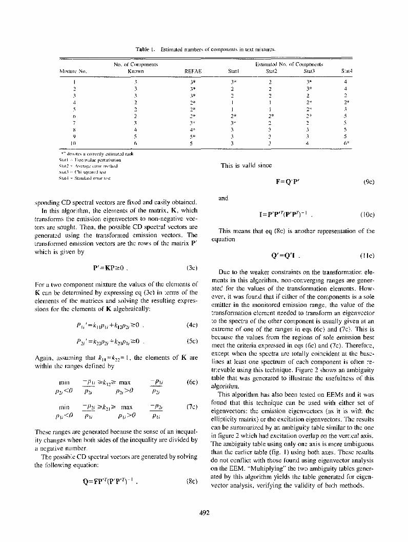
Table 1. Estimated numbers ot componems in text mixtures.

No. of Components Estiiiuiat io. or componemsMixture No. Known REFAE Stalt Stau Slai3 Sca4

I 3 38 38 2 3* 42 3 3' 2 2 3* 43 3 3' 2 2 2 24 2 28 1 2* 25 2 2* 1 1 2* 3

,. 2 2* 2* 28 28 53 3¢ 3* 2 2 5

s 4 4* 3 3 3 59 5 58 3 3 3 5

1I 6 5 3 3 4 68

+ i doI..e. d i rocily o i ... cii2L rankslit I I-l cmifllU pIxmtrblian.l;, l l = Acrn .zc ,i , i 1,..:li..i.i,.i3 < (i 1uq,,.i.d i1

Si,i14 -SiinuIlaid error loc

This is valid since

sponding CD spectral vectors are fixed and easily obtained.In this algorithm, the elements of the matrix, K, which

transforms the emission eigenvectors to non-negative vec-tors are sought. Then, the possible CD spectral vectors aregenerated using the transformed emission vectors. Thetransformied emission vectors are the rows of the matrix P'which is given by

and

1=p'ptT(p'pT)-I -

This means that eq (Sc) is anotherequation

Q'=Q'I -

(IOc)

representation of the

(1 Ic)

P'=KPŽ0 . (3cj

For a two component mixture the values of the elements ofK can be determined by expressing eq (3c) in terms of theelements of the matrices and solving the resulting expres-sions for the elements of K algebraically:

Pj, ' =kj Ipji +kIP2zO 20 r(4c)

Pj' =Ik2,, +k 21pliŽ0 . (5c)

Again, assuming that k1i=k,, = 1 the elements of K arewithin the raiges defined by

mini Pi ak-1 12 max

P, <(0 P2Ž P2i >°

mmill -Pni 2k, max

P7j< 0 Pui Pi1>O

Pli

P2r

-PiPli

These ranges are generfated because the sense of an inequal-ity changes when hoth sides of the inequality are divided by

a negative nlmberThe possible CD spectral vectors are generated by solving

the following equation:

Q=FP`(P'P)- . (Sc)

Due to the weaker constraints on the transformation ele-ments in this algorithm, non-converging ranges are gener-ated for the values of the transformation elements. How-ever, it was found that if either of the components is a soleemitter in the monitored emission range, the value of the

transformation element needed to transform an eigenvectorto the spectra of the other component is usually given at anextreme of one of the ranges in eqs (6c) and (7c). This isbecause the values from the regions of sole emission bestmeet the criteria expressed in eqs (6c) and (7c). Therefore,except when the spectra are totally coincident at the base-lines at least one spectrum of each component is often re-trievable using this technique. Figure 2 shows an ambiguitytable that was generated to illustrate the usefulness of thisalgorithm.

This algorithm has also been tested on EEMs and it wasfound that this technique can be used with either set ofeigenvectors: the emission eigenvectors (as it is with theellipticity matrix) or the excitation eigenvectors. The resultscan be summarized hy an ambiguity table similar to the onein figure 2 which had excitation overlap on the vertical axis.The ambiguity table using only one axis is more ambiguousthan the earlier table (fig. I) using both axes. These resultsdo not conflict with those found using eigenvector analysison the EEM. "Multiplying" the two ambiguity tables gener-ated by this algorithm yields the table generated for eigen-

vector analysis, verifying the validity of both methods.

492

F=Q'P' (9c)

Emission Overlap

Figure 2-Ambiguity Table of Two-Component Ellipticity Matrix

Conclusions

This manuscript has provided an overview of qualitativeanalysis techniques developed for matrix formatted fluores-cence data. Qualitative analysis of matrices was shown togenerally consist of three basic procedures: rank estimation,determination of unknown component spectra, and screen-ing of expected compounds. The techniques outlined hereonly addressed the first two phases of the problem but theyrepresent only a portion of the methods that have beendeveloped to fill these requirements. The methods presentedhere successfully attack the stated problems within theframework of the limitations described.

Rank estimation by frequency analysis can sometimes bemore accurate than statistical methods for evaluation ofspectral data. It would be useful to develop a criterion wherethe algorithm will automatically select a useful range fordifferentiating the secondary eigenvectors from the primary.

In the present approach, eigenvector analysis and eigen-vector ratioing are limited to binary mixtures. Few realsamples are binary. These methods must be extended tohigher order mixtures.

These techniques have been developed for use with fluo-rescence data, but are generally applicable to other forms ofmatrix formatted data. Some of the algorithms require thatthe data matrix be bilinear in form; however this is a charac-teristic of many types of data. For example, diode arraydetection of liquid chromatography and absorption kinetic

data using a diode array detector are bilinear in form.Clearly, there is a need for further development in this area.

References

[l] Parker, C A., Phololuminescence of Solutions with Applicationm toPIhotoclremistv and Analytical Chemistn, American Elsevier.New York (1968).

[2] Warner, I.M.; JB. Callis, ER. Davidson, M. Gouterman, and GD.Christian, Anal. Let., 8, 665 (1965).

[3] Malinowski, ER., and DG. Howery, Factor Analysis in Chemistry,John Wiley, New York (1980).

[4] Jurs, P.C., and T. L. Isenhour, Chemical Applications of Palter,Recognition, John Wiley, New York, NY, 1975.

[5] Tinoco, 1. Jr. and D.H. Turner, J. Amz. Chent. Soc., 98(21), 6453(1976).

[6] Thomas, M.: G. Patonay and IM. Warner, work in progress.[7] Warner, lM., "The Analysis of Matrix Formatted Mulficomponent

Data," Contemporary Topics it, Analytical and Clinical Chem-istry D.M. Hercules, G.M. Hieftje, LR. Snyder and M.A.Evenson, eds., Plenum, New York (1982).

[8] Fukunaga, K.. Inlroduclion to Statistical Pattern Recognition, Aca-demic Press. New York (1972).

[9] Rossi, T.M., and ILM. Warner, Rank Determination of EmissionExcitation Matrices via Fourier Transformation of Eigenvectors,"American Chemical Society, 187th National Meeting, April 8-13,1984, St. Louis. MO.

[1t] Bloomfied, P., Fourier Analysis of Time Series: An Introduction.John Wiley and Sons, New York (1976).

[11] Neal, S.L.; C.-N. Ho and IM. Warner, "Qualitative Analysis ofMulticomiiponent Fluorescence Detected Circular DichroismData,' American Chemical Society, 187th National Meeting,April 8-13, 1984, St. Louis, MO.

493

Journal of Researct of the National Bueau of StandardsVolume 90, Number 6, November-December 1985

Some New Ideasin the Analysis of Screening Designs

George BoxUniversity of Wisconsin-Madison, Madison, WI 53705

and

R. Daniel MeyerLubrizol Corp., Wickliffe, OH 44092

Accepted: July 1, 1985

Consideration of certain aspects of scientific method leads to discussion of recent research on the role of screeningdesigns in the improvement cf quality. A projective rationale for the use of these designs tn the circumstances of fictorsparsily is advanced. In this circumstance the possibility of identification of sparse dispersion effects as well as sparselocation effect is considered. A new method for the analysis of firactional factorial designs is advanced.

Key words: factor sparsity; fractional factorial designs; screening designs; sparse dispersion; sparse location.

Humans differ from other animals most remarkably intheir ability to learn. It is clear that although throughout thehistory of mankind technological learning has taken place,although until three or four hundred years ago change oc-curred very slowly. One reason for this was that in order tolearn something - for example, how to make fire or cham-pagne - two rare events needed to coincide: (a) an informa-tive event had to occur, and (b) a person able to draw logicalconclusion and to act on them had to be aware of thatinformative event.

Passive surveillance is a way of increasing the probabilitythat the rare informative event will be constructively takennote of and is exemplified by quality charting methods.Thus a Shewhart chart is a means to ensure that possiblyinformative events are brought to the attention of those whomay be able to discover in them an "assignable cause" t11'and act appropriately.

About the Author, Paper: George Box, who is with theResearch Center for Quality and Productivity Improvementat the University of Wiconsin-Madison, and R. DanielMeyer are both Statisticians. The work they describe wassponsored by U.S. Army Contract DAAC 29-80-C-0041and National Science Foundation Grant DMS-8420968.

'Figures in hrackets indicate literature references.

Active intervention by experimentation aims, in addition,to increase the probability of an informative event acuawlloccurring. A designed experiment conducted by a qualifiedexperimenter can dramatically increase the probability oflearning because it increases simultaneously the probabilityof an informative event occurring and also the probability ofthe event being constructively witnessed. Recently there hasbeen much use of experimental design in Japanese industryparticularly by Genichi Taguchi [2] and his followers. Inoff-line experimentation he has in particular emphasized theuse of highly fractionated designs and orthogonal arrays andthe minimization of variance.

In the remainder of this paper we briefly outline somerecent research on the use of such screening designs.

1. Use of Screening Designs toIdentify "Active" Factoring

Table I shows in summary a highly fractionated two-levelfactorial design employed as a screening design in an off-line welding experiment performed by the National RailwayCorporation of Japan [2]. In the column to the right of thetable is shown the observed tensile strength of the weld, oneof several quality characteristics measured.

495

The design was chosen on the assumption that in additionto main effects only the two-factor interactions AC, AG,AH. and GH were expected to be present. On that supposi-tion, all nine main effects and the four selected two-factorinteractions can be separately estimated by appropriate or-thogonal contrasts, the two remaining contrasts correspond-ing to the columns labelled el and e, measure only experi-mental error. Below the table are shown the grand average,the 15 effect contrasts, and the effects plotted on a dotdiagram. The effects plotted on normal probability papersuggested that, over the ranges studied, only factors B andC affect tensile location by amounts not readily attributed tonoise.

If this conjecture is true, then, at least appoximately, the16 runs could be regarded as four replications of a 22 facto-rial design in factors B and C only. However, when theresults are plotted in figure I so as to reflect this, inspectionsuggests the existence of a dramatic effect of a differentkind-when factor C is at its plus level the spread of the dataappears much larger 3 than when it is at its minus level.Thus, in addition to detecting shift in location due to B andC, the experiment may also have detected what we will calla dispersion effect due to C. The example raises the generalpossibility of analyzing unreplicated designs for dispersioneffects as well as for the more usual location effects.

2To facilitate liter discussion we have set out tie design and labelled the levelssomewhat differently from 121.

3Data of this kind might be accounted for by the effect of one or mor variables

other than B that affected tensile strength only at the "plus level" of C (only when thealternative material was used), Analysis of the eight runs made at the plus level of Cdoes not support this possibility, however.

+ . e

4F40 42 44 46 4C-

2. Rationales for UsingScreening Designs

Before proceeding we need to consider the question, "Inwhat situations are screening designs, such as highly frac-tionated factorials, useful?"

2.1. Effect Sparsity. A common industrial problem is tofind from a rather large number of factors those few that areresponsible for large effects. The idea is comparable to thatwhich motivates the use in quality control studies of the"Pareto diagram." (See, for example, [31). The situation isapproximated by postulating that only a small proportion ofeffects will be 'acti'e" and the rest "inert". We call this thepostulate of effect sparsity. For studying such situations,highly fractionated designs and other orthogonal arrays[2,4,5,6] which can screen moderately large numbers ofvariables in rather few runs are of great interest. Two mainrationalizations have been suggested for the use of thesedesigns; both ideas rely on the postulate of effect sparsitybut in somewhat different ways.

2.2. Rationale Based on Prior Selection of ImportantInteractions. It is argued (see for example [71) that in somecircumstances physical knowledge of the process will makeonly a few interactions likely and that the remainder may beassumed negligible. For example, in the welding experi-ment described above there were 36 possible two-factorinteractions between the nine factors, but only four wereregarded as likely, leaving 32 such interactions assumed

0 42 44 46

040O

4 0 42 4 4

0

46 40 4 2 4 4 4 6

L

Figure 1-Tensile strength data asfour replicates of a 22 fac-tonal design in factors Band C only.

B-Drying Period

496

coi

C)

4-

negligible- The difficulty with this idea is that in manyapplications the picking out of a few "likely" interactions isdifficult it not impossible. Indeed the investigator mightjUstiiiadly protest that, in the circumstance where an exper-winent is needed to determine which first order (main) effects

are important, it is illogical that he be expected to guess inadvance which effects of second order (interactions) areillportant.

2.3. Projective Rationale Factor Sparsity. A somewhatdifferent notion is that of Jatcror sparsity. Thus suppose that,of the k factors considered, only a small subset of vaguelyknown size d, wsshose idenfit is, however, unknow tsn , will beactive in providing main effects and interactions within thesubset. Arguing as in 18], a two-level design enabling us tostudy such a system is a fraction of resolution R =d + I (orin the terminology of 161. an array of strength d) whichproduces complete factorials (possibly replicated) in everyone of the (K) spaces of d=R - I dimensions. For example.we have seen that on the assumption that only factors B andC are important. the welding design could be regarded asfour replicates of a 22 factorial in just those two factors. Butbecause the design is of resolution R =3 the same wouldhave been true for any of the 36 choices of two out of thenine factors tested. Thus the design would be appropriate ifit were believed that not more than two of the factors werelikely to be "active".

For further illustration we consider again the 16-ruti or-thogonal array of table I and. adopting a roman subscript todenote the resolutions of the design, we indicate in table 2various ways in which that array might be used. It may heshown that

(a) If we associated the 15 contrast columns of the designwith 15 factors, we would generate a 2h-'I A design providingtwo-fold replication of 22 tactorials in every one of the 105two-dimensional projections.

(b) If we associated only columns 1. 2. 4. 7. S. 8.N 13.and 14 with eight factors we would generate a 211v4 designproviding two-fold replication of 2' factorials in every oneof the 56 three-dimensional projections.

(c) It we associated only columns 1, 2. 4. 8. and I5 with

five factors we would generate a 254; design providing a 24factorial in every one of the four-dimensional projections.

(d) If we associated only columns 1 2, 4. and 8 with fourfactors we would obtain the complete 2' design from whichthis orthogonal armay was in fact generated.Designs (a), (b). and (c) would thus be appropriate forsituations where we believed respectively that not more than2. 3. or 4 factors would be active 4. Notice that intermediate

41he designs give partial covcrage ot a larger number of [actors. for::ampIc t[8l I 9161)) 56 of the 7)0 four-di ncontl projCetions of tMe 2t,4yield a oull factorial it, four variables.

Table 1. A fractional two-level design used in a welding experiment showing observed tensile strength and effects.

Kind of Welding ikdsPeriod of DryingWelded MaterialThicknessAngleOpeningCurrentWelding MethodPreheating

Factorcolumn bomber

D H eI . B GH AC A a AH e 2 AG J0 1 2 3 4 5 6 7 0 9 10 11 12 13

TensileB C strenath

14 15 kg/.a

1 + - +

2 * t _ _ _3 4 _ + _ _4 + + 1 4 -5 + - - + +t6 + + _ +7 -t _ + - +Rou d + + + - *

1O + - _ _ -

11t + _ + -_12 + + + t -13 + - -+ 414 + * - - +15 + - + -

16 + * + + +Eflect 43.0 .13 -. 15 -.30 -. 15

+ ± _ - + -F - +

- + -F - - + + +

_ _ _ _ - - - +

-~ ~ -_ + + -

* - - - * + -

- + - _ + _ + -

* + + - - - - -

+ + - + _ _ + _

- + I- + + _ _ _

+ - + + - _ -

_ - - + + + + -

_ - + + - - + *

+ - - +- + - -

- +- - + - +- - +

+- 4 + + + + + +

.40 -.03 .38 .40 --05 .43 .13 .13

_ -

- + -_ + +

I + -

+- + +

-.3 4- 4 .1

497

A:B;C:0:E:F:G:Hi:3:

43.74U.242.444.742.445.942.240.642.445.543. 640.644.040.242.546.5

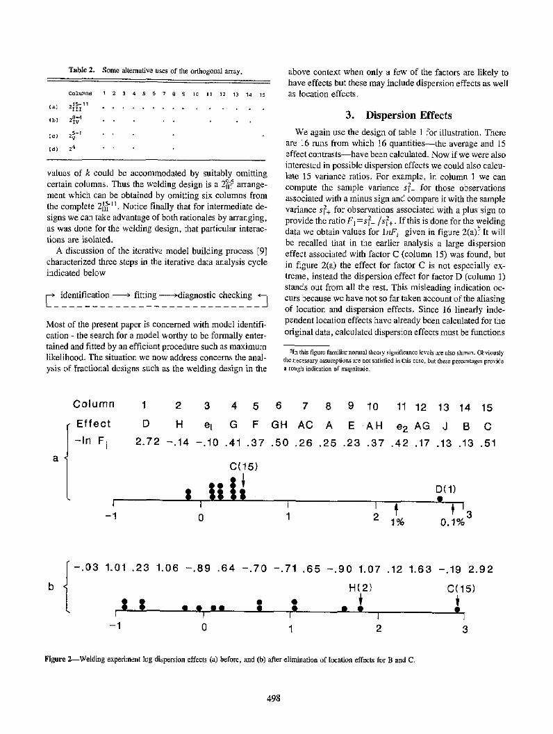
Table 2. Somne alternative uses of the orthogonal array.

coltxIrm 1 2 3 4 5 6 7 8 9 It I 1 32 1 14 15

a) 28ivII '. . I

[d}) 25"

Ed) 24

values of k could be accommodated by suitably omittingcertain columns. Thus the welding design is a 21'ji5 arrange-ment which can be obtained by omitting six columns fromthe complete 2h`' t . Notice finally that for intermediate de-signs we can take advantage of both rationales by arranging,as was done for the welding design, that particular interac-tions are isolated.

A discussion of the iterative model building process [9]characterized three steps in the iterative data analysis cycleindicated below

E identification fitting -diagnostic checking__-_______________________

Most of the present paper is concerned with model identifi-cation - the search for a model worthy to be formally enter-tained and fitted by an efficient procedure such as maximumlikelihood. The situation we now address concerns the anal-ysis of fractional designs such as the welding design in the

Column

above context when only a few of the factors are likely tohave effects but these may include dispersion effects as wellas location effects.

3. Dispersion Effects

We again use the design of table I for illustration, Thereare 16 runs from which 16 quantities-the average and 15effect contrasts-have been calculated. Now if we were alsointerested in possible dispersion effects we could also calcu-late 15 variance ratios. For example, in column I we cancompute the sample variance s - for those observationsassociated with a minus sign and compare it with the samplevariance sr2+ for observations associated with a plus sign toprovide the ratioF,=st /s2 . If this is done for the weldingdata we obtain values for InF; given in figure 2(a21 It willbe recalled that in the earlier analysis a large dispersioneffect associated with factor C (column 15) was found, butin figure 2(a) the effect for factor C is not especially ex-treme, instead the dispersion effect for factor D (column 1)stands out from all the rest. This misleading indication oc-curs because we have not so far taken account of the aliasingof location and dispersion effects. Since 16 linearly inde-pendent location effects have already been calculated for theoriginal data, calculated dispersion effects must be functions

5In this figure familiar annal theory sirificance levels ar also shown. Obviouslyhenecessry siaumptiof are not satisfed in this case but tiese rcrcenages Frevtde

a rough indication of massnitudec

1 2 3 4 5 6 7 8 9 10 11 12 13 14 15

Effect-In F.

a

D H el G F GH AC A E AH e2

2.72 -.14 -.10 .41 .37 .50 .26 .25 .23 .37 .42

C(15)

| iIIi;-1 0 1 2 1

AG J B

.17 .13 .13

D( 1)

0.1%

-.03 1.01 .23 1.06 -. 89 .64 -. 70 -.71 .65 -. 90 1.07

-1

2 la,a a so

0

H(2)

a aI1

2

.12 1.63 -.19 2.92

C(C15)

i

SI

Figure 2-Welding experiment log dispersion effects (a) before, and (b) after elimnination of location effects for B and C.

498

C

.51

b 0

I

of these. Recently [I'll a general thleory of location-dispersion abasing has been obtained for factorials and frac-tional factorials at two levels. For illus:-ation, in this partic-ULarCexample it tUnS out that the following identity exists forthe dispersion effect F1 , -hat is the F ratio associated withfactor D and hence for column 1 of the design,

Table 3. Caceulatsdeffee- frora a 2if desigr h'inaisstutrassarmr~g tiree futor and higher nade 'cittttctkas regligihleinjectionmolding expertmenL

T, = -0.7 + 1 mold terMp.

T2 = -0.1 + 2 msoisture contentF.=

t2- 3}2 + 4_5* 6ny+8F i [ i2- ;3)2+( _5)2(2+3)2 +(4+SV+(+7) 2 -(+ 9)2+(io+l 1)2+(12+ 13)2+(14+15)2

(1)

T3 = 5.5 + 3

T4 = -0.3 + 4

holding pressure

cavity thickness

booster pressureNow (see table 1) 14=lB=2. 15 and f5=C=1. 10 are the twolargest location effects, standing out from all the others. Theextreme vaLue of F] associated with an apparent dispersioneffect of factor DWl' is Largely accounted for by the squaredsum and squared difference of the location effects B and Cwhich appe;ar respectively as the fast terms in the denomina-tor and numieratot of eq (1) . A natural way to proceed is tocompute variances from the residuals obtained after elimi-nating large location effects. After such elimination the aliasrelations of eq (1) remain the same except that locationeffects from eliminated variables drop out. That is, zeros aresubstituted for eliminated variables. Variance analysis forthe residuals after eliminating effects of B and C are shownin figure 2(b). The dispersion effect associated with C (fac-tor 15) is now correctly indicated as extreme. It is shown inthe paper referenced above how, mnore generally, undercircumstances of effect sparsity a location-dispersion modelmay be correctly identified when a few effects of both kindsare present.

4. Analysis of UnreplicatedFractional Designs

Another important problem in the analysis of unreplicatedfractional designs and other orthogonal arrays concerns thepicking out of "active" factors. A serious difficulty is thatwith unreplicated fractional designs no simple estimate ofthe experimental error variance against which to judge theeffects is available.

In one valuable procedure due to Cuthbert Daniel [11,123effects are plotted on normal probability paper. For itustra-dton table 3 shows the calculated effects from a 2tsV designused in an experiment on injection molding [13, p. 371].These effec:s are plo::ed on normat] prtab-ity paper infigs-e 3.

Art a erraive lB aw2 siat Epprach 1] 4 is as ho.- aws: letT11,72 .,7i be standardizedc' effects with

Tl = e if effect inert

Tj =e +±ri if effect active

OFP lhne-hwl andt mnied tsso and hue sleld designsft eo cxampit, this analysisis arnied eat after the effects are scaled so that they all have equal variances.

= -0.1 + 6 cycle inte

0.6 & 7

ve =

gate size

1.2 + a screw speed

T9 = Tf 2 a -0E 6+ 1.2 + 3.7 - 4.8 + 5.6

TIO 2 St13 s 0.9 + 1.3 + 2.7 + 4.6 + 5.8

T11 . T1.4 5 -0.4 4 1.4 + 2.8 + 3.6 + 5.7

212 a1.5 s 4.6 + 1.5 + 2.6 + 3.8 + 4.7

E14 - T1.7 = -0.2 + 1.7 + 2.3 + 6.6 + 4.5

T15 = Tl. = -0.6 + 1.6 + 2.4 + 3.5 + 6.7

-4

8 12

-S __et-- - __----_-_ L

4-2 0 6

Filgun 3-Normal plot of effects. tnjectioit molding experiment.

499

I

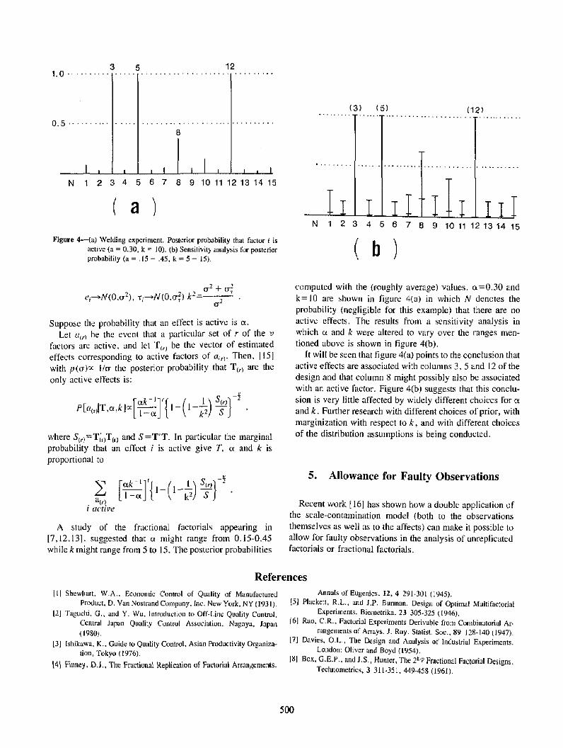
3 5

I I

(3) (5)

''''''.. 11''-.--T

I i I

1 2 3 4 5 6 7 8 9 10 11 12 13 14 15

TI I I TI L I ITN 1 2 3 4 5 6 7 8 9 10 11 12 13 14 15

Figure 4 -(a) Welding experiment. Posterior probability that factor i isactive (a = 0.30, k = tO). b) Sensitivity analysis for posteriorprobability (a = .15 - .45, k = 5-15). ( b )

e N.c2), r; -N!3.a) 2 2=! 2

Suppose the probability that an effect is active is a.Let al,.) he the event that a particular set of r of the v

factors are active, and let Tf,) be the vector of estimatedeffects corresponding to active factors of a1,). Then, [15]with p(a¢c I/a the posterior probability that T11) are theonly active effects is:

P[a r)IT, o~k ix f W { -- ) sP~atl~aitlt l-am { - k2) 5

where S,,)=T r)T(,) and S=T'T. In particular the marginalprobability that an effect i is active give T, a and k isproportional to

a 1,)i tc tie

ak I 1 _{ _|) s(I-al V 2) 51

A study of the fractional factorials appearing in17,12.13]. suggested that u might range from 0.15-0.45while k might range from 5 to 15. The posterior probabilities

computed with the (roughly average) values. a=0.30 andk1=10 are shown in figure 4(a) in which N denotes theprobability (negligible for this example) that there are noactive effects. The results from a sensitivity analysis inwhich a and k were altered to vary over the ranges men-tioned above is shown in figure 4(b).

It will be seen that figure 4(a) points to the conclusion thatactive effects are associated with columns 3. 5 and 12 of thedesign and that column 8 might possibly also be associatedwith an active factor. Figure 4(b) suggests that this conclu-sion is very little affected by widely different choices for aand k. Further research with different choices of prior, withmarginization with respect to k, and with different choicesof the distribution assumptions is being conducted.

5. Allowance for Faulty Observations

Recent work E 16] has shown how a double application ofthe scale-contamination model (both to the observationsthemselves as well as to the affects) can make it possible toallow for faulty observations in the analysis of unreplicatedfactorials or fractional factorials.

References111 Shewliart. W.A.. Economic Control of Quality of Manufactured

Product, D. Van Nostrand Company. Inc. New York, NY (1931).121 Ilagucli., G.., and Y. Wu. Introduction to Off-Line Quality Control,

Central Japun Quality Control Association. Nagoya, Japan(1980).

131 Ishikawa. K.. Guide to Quality Control. Asian Productivity Organiza-tion, Tokyo 0976).

141 Finney, D.T, The Fractionia Replication of Factorial Arrangements.

Annals of Eugenics. 12, 4 291-301 (1945).151 Plackett, R.L., and IP. Burman. Design of Optimal Muitifactorial

Experiments. Bionetrika, 23 305-325 (1946).[61 Rao, C.R., Factorial Experiments Derivable from Conbinatorial Ar-

rungements of Arrays. J. Roy. Statist. Soc., 89 128-140 (1947).17] Davies, OL., The Design and Analysis of Industrial Experiments.

London: Oliver and Boyd (1954).181 Box, G.E.P., and IS., Hunter, The 2 k p Fractional Factorial Designs.

Technometrics, 3 311-351, 449-458 (1961).

500

t .o . .......

0.5 -- - - -B

I I

N

(12)

( a )T

12

I I " .......

Vijayan Nair

AT&T Bell Laboratories

and

Michael Frenklach

Department of Materials Science and EngineeringPennsylvania State University1

Nair: The paper by Box and Meyer deals with someinteresting problems that arise in the off-line quality con-trol methods introduced by Taguchi (see Taguchi andWu [Ilfj. My comments will be restricted to the firstpart of the paper, viz. estimating dispersion effects.

1) Estimating dispersion effects for quality controlIn industrial experiments designed to detect important

factors that affect the quality of a manufacturing/production process, the estimation of dispersion effectsis as important as the estimation of location effects. Infact in situations where there are readily identifiablesignal factors (see [1]), the primary goal is in estimatingdispersion effects. The location effects, in this case, playthe role of nuisance parameters. Le6n, Shoemaker andKackar [2] offer an excellent discussion of the statisticalformulation of the parameter design problem in indus-trial experiments.

2) Effect sparsityThe Box-Meyer techniques exploit the notion of ef-

fect sparsity to obtain "replicates" in an unreplicatedexperiment. It is likely that in most cases only a fewfactors are highly significant. However, in many situ-ations, one could also expect many of the other factorsincluded in the experiment to have sizeable effects. Thisis particularly true when a fair amount of the informa-tion about the process is known and is used in the selec-tion of the factors. In such situations, one could notreasonably expect to estimate both location and dis-persion effects from an unreplicated experiment.

' Michaad Frenklacl's contribution to the subjec stems from work performedin the Departnsent of Chemical Engineering, Louisiana State University.

2 Figures in brackets indicate literature references.

3) When to log?Box suggests using log[S 2(i-)/S 2Q +)1 as a pre-

liminary estimate of the dispersion effects. An alterna-tive method would be to take log of the squared re-siduals and do ANOVA with an additive model for thelog of the scale parameters. This is the type of analysisusually done in experiments with replications. Some ef-ficiency calculations suggest that the Box-Meyer anal-ysis is more efficient when there are only a few largedispersion effects and less efficient when there are many.

4) IteratingIt is possible that during the first step of the iteration

(which does an unweighted analysis) some significantlocation effects are not detected. So after the dispersioneffects are estimated, the location model should be re-fitted for all the factors.

5) TransformationsIn replicated experiments, the quasi-likelihood mod-

els of Nelder and Pregibon [3] allow one to determinethe transformations under which the location effects andthe scale effects are approximately additive.

References

[Il Taguchi, G., and Y. Wu, Introduction to off-line quality control.Central Japan Quality Control Association (1980).

[2] Le6n, R. V.; A. C. Shoemaker and R. N. Kackar, Performancemeasures independent of adjustment: An alternative to Tag-uchi's signal to noise ratio. AT&TBeIl Laboratories TechnicalMenmorandurn (1985).

[3] Nelder, J A., and D. Pregibon, Quasi-lilkelihood models and dataanalysis. Biometrika (to appear).

501

Frenklach: Professor Box presented a method ofanalysis of factorial designs for detection of main effectsand faulty observations. The approach is analytical andprovides numerical measures for what previously hasbeen approached graphically. The availability of theanalytical algorithm is important for computerization ofthe analysis.

The central hypothesis of the method is what theauthors call effect sparsity, which states that usuallyonly a small number of input and control process vari-ables would have a significant effect on the processresponse(s). This situation appears to be true not only inexperimental environments but also in computer mod-eling of various industrial processes and natural phe-nomena. Mechanistic models usually take the form ofdifferential equations for which no analytical solution isavailable. The model may contain a large number of(physical) parameters and it is not always obvious froma simple inspection of the computational results whateffect each parameter has on a given response or re-sponses. Sensitivity analysis has been used to reveal thisinformation. Among other techniques, the use of screen-ing factorial designs for sensitivity analysis of computermodels has been suggested by Box et al. 1978; Frenklach1984; Frenklach and Bornside, 1984; Miller and Fren-klach, 1983; and Morris and Mitchell, 1983 [1-5].

The present experience with chemical kinetic mod-eling, for example, is as follows. Due to technical diffi-culties of instrumentation, there are only a few experi-mental responses available, typically one or two. The

cases studied indicate that it is a very small number ofchemical reactions, out of hundreds of reactions com-prising the model, whose rate coefficient values, withintheir uncertainty intervals, have significant or "active"effects on the experimentally verifiable model re-sponses. These are exactly the conditions of effect spar-sity discussed above. Thus, the method presented byBox is well-suited not only for "real" experimentation,but also for computer modeling.

Computations, however, do not have random errors.Does this fact simplify and economize the analysis?Should special methods and designs be developed orexisting ones modified for a most efficient use in screen-ing analysis of computer models?

References

[11 Box, 0. E. P.; W. C. Hunter and J. S. Hunter, Statistics forExperiments. An Introduction to Design, Data Analysis,and Model Building, Wiley, New York, pp. 429-432 (1978).

[21 Frenklach, M., Modeling, Combustion Chemistry (Edited by W.C. Gardiner, Jr.), Springer-Verlag, New York, Chap. 7(1984).

[3] Frenklach, M., and D. E. Bornside, Shock-initiated ignition in

methane-propane mistures, Combust. Flame 56, 1-27 (1984).[4] Miller, D., and M. Frenklach, Sensitivity analysis and parameter

estimation in dynamic modeling of chemical kineties, Int. J.Chem. Kinet. Is, 677-696 (1983).

151 Morris, M. D., and T. J. Mitchell, Two-level multifactor designsfor detecting the presence of interaction, Technm. trics 25,345-355 (1983).

502

Journal of Rcsearch of the National Bureau of StancardsVolume 90, Number 6, November-December 1985

Polymers and Random WalksRenormalization Group Descriptionand Comparison With Experiment

Karl F. FreedThe University of Chicago, Chicago, IL 60637

Accepted: July 1, 1985

Although real polymers involve the sequential addition of monomers having fixed bond lcngrhs, fixed bond anglesand some freedom of rotation about single bond, the properties of polymers over large length scales can be modeledby treating the polymer configuration as that of a random walk formed by the monomer units. Serious complicatonsarise in the theoretical description of these polymers because of excluded volume constraints which prohibit differentmonomers from occupying the same position in space. This polymer excluded volume problem has been modeled interms of a simple continuous random walk with short range repulsive interactions. The expansion of polymer propertiesin this repulsive interaction can readily be shown by dimensional analysis to involve an expansion in a large parameter,in the limit of long polymers. The renormalization group method is utilized as a systematic means for resuming thisdivergent perturbation expansion. The theory proceeds by analytically continuing the treatment to continuous range ofspatial dimensionalities to expose and regularize the singularities in the analytically continued theory. The renormaliza-tion group approach is described from a heuristic physical standpoint and extensive comparisons arc provided to showhow it quantitatively reproduces vast amounts of dilute solution polymer properties with no adjustable parameters.

Key words: experiment comparison; modeling; monomer units; polymer properties: random walk: repulsive interaction.

The study of the configuration statistics of polymers indilute solutions presents problems of interest to analyticalchemists, chemical physicists, engineers and applied mathe-maticians. Roughly half of the American chemical industryis involved with polymers, and analytical chemists are con-cerned with the characterization of their properties. Dilutesolution physical properties are used to determine themolecular weight and general shape and architecture of thepolymer. Hence, the availability of a quantitative theoreticaldescription of the dependence of dilute solution physicalproperties on solvent characteristics, molecular weight,temperature, and branching is an important aid in character-izing and understanding the properties of polymers.

About the Author, Paper: Karl F. Freed is with theUniversity of Chicago's James Franck Institute and Depart-ment of Chemistry. The work he describes was sponsored inpart by the National Science Foundation.

The interest of polymers to applied mathematicians lies intheir mathematical description in terms of interacting ran-dom walks.[t]' This mathematical representation of a poly-mer chain can be motivated by visualizing the polymer as asequence of bonded monomer units. Each new monomer,added to the chain, is attached by a chemical bond of fixedlength, generally having fixed bond angles with respect tothe previous bond. However, there is considerable freedomof rotation about the individual bonds thereby generating alarge number of configurations for this idealized randomwalk polymer model [21. The individual bond angle rota-tions represent random variables describing the chain con-figurations, so that when the number of these random vari-ables, corresponding to the possible bond-vectors, gets largeenough, the central limit theorem requires that the probabil-itv distribution for a vector between the ends of the chainmust tend to a limiting Gaussian [1,2]. The random walk

'Figures in brackets indicate literature references.

503

configurations of an idealized polymer permit two differentsegments of the polymer to occupy the same position inspace, something which is not possible for real polymermolecules. Hence, real polymers are described in terms of

interacting random walks with an excluded volume interac-tion prohibiting the multiple occupancy of monomers at thesame place in space.

Experimental methods of polymer characterization in-clude light scattering, osmometry, sedimentation, viscome-try. etc. When the polymer concentration c approaches zero;osmometry provides the determination of the molecularweight Ml of the polymer, while small angle light scatteringyields the polymers' radius of gyration RG. The limitingslope of the light scattering intensity as a function of concen-tration in the zero angle limit provides the polymer secondvirial coefficient A2 which measures the effective volumethat a polymer excludes to other chains. The translationaldiffusion coefficient D is written for c-0 using Stokes' andEinstein's laws in terms of hydrodynamic radius RH by

D=kTI6l1rRH where T is the absolute temperature, k isBoltzmann's constant and -lu is the solvent viscosity. If 7]

designates the viscosity of the polymer solution, the intrin-sic viscosity E'n)=l'O(m-To)/c gives another measure ofthe volume occupied by a single polymer chain.

All of these large scale observables for polymers providedifferent measures of the overall size and shape of the poly-mer. These properties are often found to vary with the poly-mer molecular weight in the form of a power law KM"where the proportionality factors K and the exponents adepend on the polymer, solvent, and temperature as wellbeing slowly varying functions of M. It is the goal of acomprehensive quantitative theory of polymers [3] in dilutesolution to explain the variation of K and a with thepolymer-solvent system and the temperature over the fullexperimentally accessible range.

Because large scale polymer properties like RG0 A2, D and(11) are measures of large scale or long wave length polymerproperties, the theoretical description of these polymerproperties does not require a detailed treatment of the shortrange microscopic details of the polymer such as the specificbond lengths, bond angles and hindered rotation potentials.Rather, it suffices to employ apparently simple models tocapture the essential large length scale characteristics oflong chain molecules 13-7].

The above noted popular random flight model of poly-mers treats the chain as having a set of effective monomerunits sequentially number 0, 1, ... , at the spatial positionsro, rl, ... , r,. Because the properties of interest involvelarge distance scales and implicitly large n, the central limittheorem allows us to take the individual bonds to have aneffective Gaussian length distribution [1,2] with an rms

value of i. The excluded volume interaction is modeled byintroducing a short range repulsive contribution to the en-

ergy when a pair of segments occupies the same position in

space. This model then describes the dimensionless (free)energy associated with a chain configuration {rkJ of theform [ [-4]

H/kT=(d(2j2) 3 jr, rj_112zi=l

n

+(%/2) > 6iri-ri1 j= 0

(I)

where ij3 is the volume excluded by an effective segmentdue to the presence of another. The spatial dimensionality isd, and it is convenient to consider the description of poly-mers as a function of the dimensionality of space wherenormal solutions involve d=3 while the case d=2 is associ-ated with polymers at a surface or an interface.

The probability distribution function for the chain config-uration {rk} is governed by the Boltzmann factor exp(-H!kT. Each of the monomer units in (1) describes the centerof mass position of a collection of several actual monomersin the real polymer. This coarse -raining is permissiblebecause we are interested in long wavelength polymer prop-erties. The first term on the right hand side in (i), therefore,represents the entropy of the polymer chain configurationassociated with the many internal degrees of freedom inthese coarse grain effective units [1-3]. Retention of onlythis term yields the simple Gaussian chain model of poly-mers at the theta temperature, a simple model for which thelong wavelength polymer properties are easily evaluated.The entropic or elastic energy accounts in the model for theconnectivity of the polymer chain.

The second term on the right hand side of (1) contains apairwise sum over all the effective monomers and therebyconverts the simple Gaussian chain model into a true many-body problem. The complexity of the treatment of excludedvolume is readily seen by expanding exp(-HikT) of (l) inpowers of Por and evaluating polymer properties as a formalpower series in Po. This excluded volume perturbationtheory is readily shown [2-7] to be an expansion in thedimensionless quantity P3ol-dn"2 with e=4-d. Hence, forhigh molecular weight polymers where n is large, the expan-sion is in a large parameter as long as 3ol -d<n cEo 2 and d<4.

Consequently, the perturbation theory alone is of little useexcept very near the theta temperature where the empirical

Po vanishes. The power law dependence of polymer proper-ties on the molecular weight also indicates the difficulty ofusing these perturbation expansions in powers of Po since itis hard to see how a few terms in such an expansion, in alarge parameter, can simply be resumed in order to providethe empirically observed nonanalytic power law dependencewith fractional and often continuously varying exponents as

a function of temperature.

504

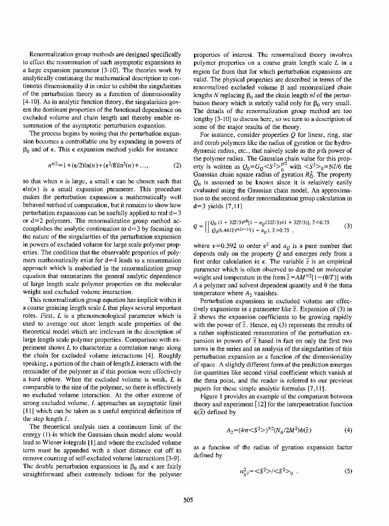
Renormalization group methods are designed specificallyto effect the resummation of such asymptotic expansions ina large expansion parameter [3-10]. The theories work byanalytically continuing the mathematical description to con-tinuous dimensionality d in order to exhibit the singularitiesof the perturbation theory as a function of dimensionality[4-10]. As in analytic function theory, the singularities gov-ern the dominant properties of the functional dependence onexcluded volume and chain length and thereby enable re-summation of the asymptotic perturbation expansion.

The process begins by noting that the perturbation expan-sion becomes a controllable one by expanding in powers ofPo and of E. This e expansion method yields for instance

n"l2= 1 +(E/2)ln(n)+(E2/8)1n2(n )+..., (2)

so that when n is large, a small e can be chosen such thatEln(n) is a small expansion parameter. This proceduremakes the perturbation expansion a mathematically wellbehaved method of computation, but it remains to show howperturbation expansions can be usefully applied to real d=3or d=2 polymers. The renormalization group method ac-complishes the analytic continuation to d=3 by focusing onthe nature of the singularities of the perturbation expansionin powers of excluded volume for large scale polymer prop-erties. The condition that the observable properties of poly-mers mathematically exist for d=4 leads to a resummationapproach which is embodied in the renormalization groupequation that summarizes the general analytic dependenceof large length scale polymer properties on the molecularweight and excluded volume interaction.

This renormalization group equation has implicit within ita coarse graining length scale L that plays several importantroles. First, L is a phenomenological parameter which isused to average out short length scale properties of thetheoretical model which are irrelevant in the description oflarge length scale polymer properties. Comparison with ex-periment shows L to characterize a correlation range alongthe chain for excluded volume interactions [4]. Roughlyspeaking, a portion of the chain of length L interacts with theremainder of the polymer as if this portion were effectivelya hard sphere. When the excluded volume is weak, L iscomparable to the size of the polymer, so there is effectivelyno excluded volume interaction. At the other extreme ofstrong excluded volume, L approaches an asymptotic limit[II] which can be taken as a useful empirical definition ofthe step length 1.

The theoretical analysis uses a continuum limit of theenergy (I) in which the Gaussian chain model alone wouldlead to Wiener integrals [I] and where the excluded volumeterm must be appended with a short distance cut off toremove counting of self-excluded volume interactions [3-9].The double perturbation expansions in 0o and e are fairlystraightforward albeit extremely tedious for the polymer

properties of interest. The renormalized theory involvespolymer properties on a coarse grain length scale L in a

region far from that for which perturbation expansions arevalid. The physical properties are described in terms of therenormalized excluded volume 3 and renormalized chainlengths N replacing 130 and the chain length nI of the pertur-bation theory which is strictly valid only for 0I very small.The details of the renormalization group method are toolengthy [3-10] to discuss here, so we turn to a description ofsome of the major results of the theory.

For instance, consider properties Q for linear, ring, starand comb polymers like the radius of gyration or the hydro-dynamic radius, etc., that naively scale as the pth power ofthe polymer radius. The Gaussian chain value for this prop-erty is written as QO=GQ<S2>ol 2 with <S 2 >O=Nll6 theGaussian chain square radius of gyration RG. The propertyQ0 is assumed to be known since it is relatively easilyevaluated using the Gaussian chain model. An approxima-tion to the second order renormalization group calculation ind=3 yields [7,11]

Q = {[Qo (I + 32z/3)P'8[l + aQ(32zl3)1(t + 32z/3)], z<0.75

Qo(6.441t( 2 v-)(It + aQ), 7>0.75 (3)

where v=0.592 to order E2 and aQ is a pure number that

depends only on the property Q and emerges only from afirst order calculation in e. The variable z is an empiricalparameter which is often observed to depend on molecularweight and temperature in the form z =AM t12[1 -(O/T)] withA a polymer and solvent dependent quantity and 0 the thetatemperature where A2 vanishes.

Perturbation expansions in excluded volume are effec-tively expansions in a parameter like i. Expansion of (3) ini shows the expansion coefficients to be growing rapidlywith the power of z. Hence, eq (3) represents the results ofa rather sophisticated resummation of the perturbation ex-pansion in powers of i based in fact on only the first twoterms in the series and an analysis of the singularities of thisperturbation expansion as a function of the dimensionalityof space. A slightly different form of the prediction emergesfor quantities like second virial coefficient which vanish atthe theta point, and the reader is referred to our previouspapers for these simple analytic formulas [7,11].

Figure I provides an example of the comparison betweentheory and experiment [ 12] for the interpenetration function+(i) defined by

A2= (4 ir<S 2>)3 12(NA 12M2 )d!(7) (4)

as a function of the radius of gyration expansion factordefined by

oU2,=<S2>1<SI>, . (5

505

T1

1 2 3 43

better than that presented in figure 1. The situation is some-what more complicated for the dynamical properties RH and[q] where our theoretical calculations show that the effec-tive exponents a in good solvents often depend on an addi-tional parameter, called the draining parameter [13]. Webelieve that the success of this renormalization group de-scription of the excluded volume dependence of dilute solu-tion properties will enable us to describe polymer propertiesin a variety of mathematically more complicated and physi-cally very interesting situations such as the properties ofpolymers in interaction with a surface or interface, the prop-erties of polyelectrolyte solutions where polymers have adistribution of charges and there are small counter ions insolution, and the properties of polymer mixtures in solution.

Figure I-Comparison of theories 121 and experiment for variation of k[with a3 [31. The figure is reproduced from Yamakawa [2] with theparameter free RG predictions added. Data points from Norisuye et al.

[141 are O for polychloroprene (PC) in CCI4 at 250C, 6 for PC inn-butyl acetate at 250C, and C for PC in transdecalin at various temper-atures. Similar data 115] and agreement with theory is available forpolyisobutylene, polystryrene and poly-p-methylstyrene in various sol-vents. The curves (l)-(3) represent older theories as reviewed by Ya-makawa [21.

The renormalization group prediction is given by the solidline marked RG, whereas the other lines represent older

theories [2] which lack systematic mathematical guidanceand therefore which are unable to predict the physicallyobvious fact that l must lead to a universal value in the limitof large chain expansion or equivalently large excluded vol-

ume interaction z.An important feature of figure I is that the theoretical

curve is obtained with absolutely no adjustable parameters,and that it is also derived using purely analytical methods.Hence, its derivation is in the true spirit of analytical chem-istry, using the methods of mathematical analysis to pro-

vide quantitative descriptions of the properties of chemicalsystems. This type of work merges the disciplines of analyt-ical chemistry and applied mathematics and is therefore at

the heart of the goals of chemometrics.Renormalization group calculations have been performed

for a wide range of polymer properties [ 12] in dilute solu-tions for linear, ring, star, and block copolymers. The agree-ment between theory and experiment is generally as good or

I am grateful to Jack Douglas for comments on the

manuscript.

References

[11 A more mathematically oriented introduction to polymers as interact-ing random walks is given in K.F. Freed, Ann. Prob. 9, 537(1981), a paper which predates our current work with the morepowerful renormalization group methods.

[21 See, for instance, H. Yamakawa, Modern Theory of Polymer Solu-tions (Harper and Row, New York, 1971) and references therein.

[31 Freed, K.F., Accts. Chem. Res. 18, 38 (1985).[4] Oono, Y., T. Ohia and K.F. FreedJ. Chem. Phys. 74, 6458 (1971).[51 Oono, Y., and K.F. Freed, J. Phys. A 15, 1931 (1982).[61 Kholodenko A.L., and K.F. Freed, J. Chem. Phys. 78, 7390 (1983).[7) Douglas, J.F., and K.F. Freed, Macromolecules 17, 1854 (1984).[81 Amit, D.J., Field Theory. The Renornalization Group and Critical

Phenomena (McGraw-Hill, New York, 1978).191 Ramond, Field Theory, A Modern Primer (Benjamin/Cummings.

Reading, Mass., 1981).[10] Freed, K.F., Renormalization Group Theory of Macromolecules

(Wiley, to be published).[11] Douglas, J.F., and K.F Freed, Macromolecules 15, 1800 (1983).1121 Douglas, J.F., and K.F. Freed, Macromolecules 17, 2344 (1984); 18,

201 (1985).[13] Douglas, J.F., and K.F. Freed, Macromolecules 17, 2354 (1984).[14] Norisuye, T., K. Kawahara, A. Teramoto and H. Fujita, J. Chem.

Phys. 49, 4330 (1968); K. Kawahara, T. Norisuye and H. Fujita,J. Chem. Phys. 49, 4339 (1968).

[151 Berry, G.C., J. Chem. Phys. 44, 4550 (1966); G. Tanaka, S. Imaiand H. Yamakawa, J. Chem. Phys. 52, 2639 (1970); T. Mat-sumoto, N. Nishioka and H. Fujila. J. Polym. Sci. 10, 23 (1972).

506

Journalof Research of the National Bureau of StandardsVoL 90, No. 6, November-December 1985

Fourier Representationsof Pdf's Arising in Crystallography

George H. Weiss

National Institutes of Health, Bethesda, MD 20205

and

Uri Shmueli

Tel-Aviv University, Ramat-Aviv 69978, Tel-Aviv, Israel

Accepted: June 24, 19V5

A survey is given of some recent calculations of univariate and multivariate probability density functions(pdfs) of structure factors used to interpret crystallographic data. We have found that in the presence ofsufficient atomic heterogeneity the frequently used approximations derived from the central limit theorem in theform of Edgeworth or Gram-Charlier series can be quite unreliable, and in these cases the more exact, butlengthier, Founrer caiculations must be made.

Key words: characteristic functions; direct methods of phase determination; Fourier series; intensity statistics.

Few scientific disciplines depend so heavily on tech-niques based on the central limit theorem and associatedexpansions in orthogonal polynomials as does crys-tallography. Ever since the pioneering work of Wilson[1,2 ],' and Karle and Hauptman [3-5], the central limittheorem has played a vital role in translating crys-tallographic scattering data into structural informationand, indeed, it is built into many computer routines forthis purpose. As we will show, when the central limittheorem is applied to data from unit cells with a consid-erable variation in the atomic weights of the constituentatoms it can lead to serious qualitative errors. That this

About the Authors: George H. Weiss is an appliedmathematician and Uri Shmueli is a chemist.

is true is well known to crystallographers who havemade heavy use of Edgeworth and related expansions tocorrect zeroth order approximations based on the cen-tral limit theorem [5,61. It is not generally appreciated,however, that serious errors can persist even with thesecorrection terms, provided that atomic heterogeneity issufficiently great. This suggests the value that may beattached to exact results when these are available andare readily computed. This paper reports on recent ef-forts we and several collaborators 17-11] have made inthis direction.

Two general classes of probabilistic methods are usedto deduce structural information from radiation in-tensity diffracted from crystals, the so-called intensitystatistics and direct methods of phase determination. Inorder to make this exposition self-contained, we willsketch how such information can be derived from data

507

'Figures in brackets indicate literature references.

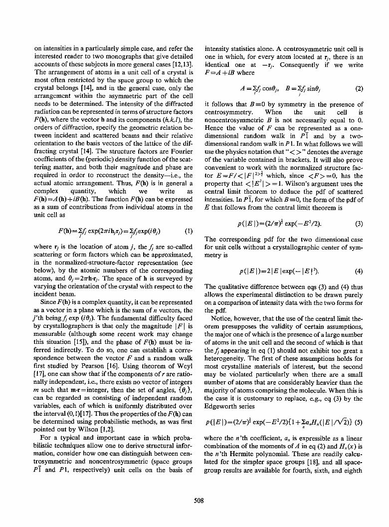
on intensities in a particularly simple case, and refer theinterested reader to two monographs that give detailedaccounts of these subjects in more general cases [12,13].The arrangement of atoms in a unit cell of a crystal ismost often restricted by the space group to which thecrystal belongs [14], and in the general case, only thearrangement within the asymmetric part of the cellneeds to be determined. The intensity of the diffractedradiation can be represented in terms of structure factorsF(h), where the vector h and its components (h,k,l), theorders of diffraction, specify the geometric relation be-tween incident and scattered beams and their relativeorientation to the basis vectors of the lattice of the dif-fracting crystal [14]. The structure factors are Fouriercoefficients of the (periodic) density function of the scat-tering matter, and both their magnitude and phase arerequired in order to reconstruct the density-i.e., theactual atomic arrangement. Thus, F(h) is in general acomplex quantity, which we write asF(h) =A (h) + iB (h). The function F(h) can be expressedas a sum of contributions from individual atoms in theunit cell as

F(h)= =Xfj exp(27rihjrj)= Yif oexpOi)

intensity statistics alone. A centrosymmetric unit cell isone in which, for every atom located at rp, there is anidentical one at -rp Consequently if we writeF=A +iB where

A=X3fjcosO, B=XfsinOQ (2)

it follows that B sO by symmetry in the presence ofcentrosymmetry. When the unit cell isnoncentrosymmetric B is not necessarily equal to 0.Hence the value of F can be represented as a one-dimensional random walk in P1I and by a two-dimensional random walk in P 1. In what follows we willuse the physics notation that " < > " denotes the averageof the variable contained in brackets. It will also proveconvenient to work with the normalized structure fac-tor E=F/<1F2'>l which, since <F>=0, has theproperty that < I Et I > = 1. Wilson's argument uses thecentral limit theorem to deduce the pdf of scatteredintensities. In P 1, for which B 9O, the form of the pdf ofE that follows from the central limit theorem is

p(IE I)=(2/1r)l exp(-E2 /2).(1)

where rj is the location of atom j, the fj are so-calledscattering or form factors which can be approximated,in the normalized-structure-factor representation (seebelow), by the atomic numbers of the correspondingatoms, and O1 =27rh r1 . The space of h is surveyed byvarying the orientation of the crystal with respect to theincident beam.

Since F(h) is a complex quantity, it can be representedas a vector in a plane which is the sum of n vectors, thej'th being fj exp (iQOj). The fundamental difficulty facedby crystallographers is that only the magnitude IFI ismeasurable (although some recent work may changethis situation [15]), and the phase of F(h) must be in-ferred indirectly. To do so, one can establish a corre-spondence between the vector F and a random walkfirst studied by Pearson [16]. Using theorem of Weyl[17], one can show that if the components of r are ratio-nally independent, i.e., there exists no vector of integersm such that m-r=integer, then the set of angles, {Oj},can be regarded as consisting of independent randomvariables, each of which is uniformly distributed overthe interval (0,1)[17]. Thus the properties of theF(h) canbe determined using probabilistic methods, as was firstpointed out by Wilson [1,2].

For a typical and important case in which proba-bilistic techniques allow one to derive structural infor-mation, consider how one can distinguish between cen-trosymmetric and noncentrosymmetric (space groupsPI and PI, respectively) unit cells on the basis of

(3)

The corresponding pdf for the two dimensional casefor unit cells without a crystallographic center of sym-metry is

p(IE I)=2IE Iexp(- IE 2). (4)

The qualitative difference between eqs (3) and (4) thusallows the experimental distinction to be drawn purelyon a comparison of intensity data with the two forms forthe pdf.

Notice, however, that the use of the central limit the-orem presupposes the validity of certain assumptions,the major one of which is the presence of a large numberof atoms in the unit cell and the second of which is thatthe fj appearing in eq (1) should not exhibit too great aheterogeneity. The first of these assumptions holds formost crystalline materials of interest, but the secondmay be violated particularly when there are a smallnumber of atoms that are considerably heavier than themajority of atoms comprising the molecule. When this isthe case it is customary to replace, e.g., eq (3) by theEdgeworth series

p(JE 1 )=(2/7r)2 exp(-E'/2)f 1 + MaœH,( E 1\/-2)1 (5)

where the n 'th coefficient, a. is expressible as a linearcombination of the moments of A in eq (2) and H,(x) isthe n 'th Hermite polynomial. These are readily calcu-lated for the simpler space groups [18], and all space-group results are available for fourth, sixth, and eighth

508

moments(19,20j. Furthermore, the Edgeworth expan-sion may also not be too useful in the presence of ex-treme heterogeneity. This is illustrated in figure 1 in

which the asymmetric unit of a cell in Pi consists of 14carbon atoms and one uranium atom, with a ratio offsapproximatelv equal to 15Q Wiith 0 or 2 nacrments theEdgeworth series fails to reproduce the maximum andthe 4 and 8 moment approximation locates the maximumquite far from its actual position. It is therefore desirableto have an exact easily computable representation forthe pdf which is robust with respect to changes inatomic heterogeneity.

Just such a representation was first suggested byBarakat in a study of the freely jointed chain as a modelfor polymer configurations [21] and of laser speckle [22].Let us write gj =f /(ZJ;'2) so that

where

a, ==f g(A)cos(rT•) oA±=r %(A (T

cClr (9)

where C(ow) is the characteristic function generated byg(A). The Fourier series in eq (8) corresponds to a sam-pling theorem [23] for pdrs with a compact support.When the unit cell is noncentrosymmetric so that B =O

in general, it is more convenient to expand the pdf of

IE I =(A2+B1)i in a Fourier-Bessel function series

(10)p(lEE mom . Dfu(yjAEJIS)

E =igj cxpirO1)=A +zB (6)

and let us set

where the yj are successive roots of Jc(y>=O and thecoefficients, DX, are

Dj = C(y/S )/I()

so that -5S <A(5S. As an example we consider thecase of a centrosymmetric unit cell for which B = 0. Thepdf of A, g(A), has the property that it can differ fromzero only in the interval S2>A2 . Within this interval wewill expand g(A) in a Fourier series:

g()=_ t{t+2- a, cos75r)} (N

C-Mc

again written in terms of the characteristic function.Two questions that require an answer relate to the

advantage of representations such as those in eqs (8) or- 10) and the feasibility of numerical evaluation of theseries. In the absence of atomic heterogeneity, or whenthere Ls a very large number of atoms in a unit cell, thecentral limit results are perfectly adequate for crys-

_I-

( a

0.50 0.75

A

1.0 0 0.25 0.50 0.75

A

Figure ta-(a) Apisoxitiationm to the exawt pdf giA) (devoted by tEe solid Rie; fec a unit cell in spzcaa group Pt coms-stm oF :4 c-anon

atoms and a single uranium atom (atomic weLght ratio [i 2:I) in the asymmetric unit, For convenience Am, has been set equal to 1L Note

that the pdf is symmetric around A =0. The approximations are a Gaussian (---) and the Gaussian corrected by two moments ( --. ). (hJ

Approximations to the same pdf as in figure la by an Edgeworth series using 4 moments (---) and s moments (.- -.).

509

S =xgj (7) (I 1)

0 0.251.0

tallographic applications. However, when there arefewer than about 40 atoms in the unit cell combined withone or two outstandingly heavy atoms, one has to con-volve the Gaussian with the appropriate pdf for theheavy atoms [12]. In principle, using the series of eqs (8)and (10) finesses this difficulty, provided that the con-vergence properties are not overwhelming. In practice,in the case of intensity statistics we have found no prob-lem in evaluating the Fourier or Fourier-Bessel functionseries, requiring no more than about 40 terms for themost extreme amounts of heterogeneity, and manyfewer terms in the absence of heterogeneity. The evalu-ation of the analogous series for direct methods canpresent much tougher numerical problems, as we willsee. Finally, a problem not so far discussed is the easewith which expressions for the characteristic functioncan be calculated. We have found that it is not toodifficult to evaluate the characteristic function for allbut a handful of space groups whose structure factor isfound in the International Tables 124]. As an example, letus write the structure factor for PI as

,'2A =2 1 gIgcoso,

where the g1 are known and the Oj are uniformly distrib-uted in (0,27r). The characteristic function is

e2C(Q)=(exp(2iei I cos;6)k

(13)

I/2==1

(12)

Again the numerical problems associated with this rep-resentation were not severe and allowed us to generalizethe theory first presented by Rogers and Wilson for theequal-atom case [9,25]. It is possible though alge-braically messy to generate the orthogonal polynomialscorresponding 10 the Rogers-Wilson pdf, but the Fou-rier series representation is relatively straightforward.One can also analyze partially bicentric structures usingthe same techniques [10.

Our present development of Fourier representationsof crystallographic pdf's has led us into the examinationof direct methods in which one is interested in the jointpdf of several, usually correlated, structure factors. Oneof the simplest examples of these is the so-called X,relationship [13,26], in which one uses the joint pdf ofE(h) and E(2h) to determine the probability that thephase of E(2h) is positive given a knowl-edge of E hl{and ?E(2h) . For simplicity we consider structures inPI letting E(h)=E and E(2h)=G. Then

p (E, G) = 14SL2 , Y 5J. "rF-(17)

cosC yE-cos(o -)

where

C'2C(&)q,ro2)= (expi idE+z i o-)IC = rLIC, (0 bc'J

in which sincewhere

(18)

./IG=2X gj cos(2OJ)

C9(x)= exp(2iag 2 cosO))(14)

exp(2iog1 cos9)a9=J.(2wg , ).

Other examples merely test one's ability to evaluate inte-grals. For example, we have recently examined the Foi-rier representation of the pdf of the intensity for a unitcell in PI in which there is an auxiliary or non-crystallographic center of symmetry located at d, so thata single atom located at rj generates one at -r, and-rjt2d [9,10]. In this case one can show that

.4A(h)=41YIg1 cos(21rh.d)cos[27rh.(r1 -d)]

and the corresponding characteristic function is

c b,. 1 I, (1 J0 (4cg, cos6j)dO.

CJ(o .co2)=9- f exp[2igj{co dcos6-+&-cos2O)J d

2 +ij(19)

where R. and 1, can be expanded in terms of Besse]functions as

R1 ( 1i,&)) =Jt(2g 1 d)J0(2gj2) + 2 I

(- 1) m J4 (2gOjW )J 2 m(2gjwt2)

(15)(20)

J(wi,oi2)= 2 2 (-1) "J+ 2(2gJ03i)J2.+1(2g.e)2 )*

From eq (18) it follows that C( :.o)R(re),,0.)16 +I(o.,o°) whereR and Ican be cocmputed from theR 1

(16) and If. The probability that G is positive given E cannow be written exactly as

510

p+(2hlh)=Rl +:) (21)

where

O X 5 tc VI os y 77E )sEniyG5 )sa§ =i1 --

r=% {1 +2LAR(5'1 )0cos( + Cos (%5)](22)

4 2 ( t)cos(PTE)cos(fiG)l .The exact eq (21) should be compared to the much

simpler approximation furnished by the use of the cen-tral limit theorem [26],

p+(2hlh) [ I1+tanhQt2 2 { GRE 2_1-

wherec./2

0. = 2= g' a'm=1 I7I

(23)

1.0

Pt

0.5F.4

4+

*+.4 F

4

+

4

,+

0.5 1 0 1.5 2.0 2.5[Ehl

I3.0

Figure 2-A graph of the exact expression for p + (2h I h), the proba-bility that the phase of E(2h) is positive, as a function of E((+ + +)compared to the approximation provided by eq (23) (the solidcurve) for a molecule with the assumed composition C,0 Kr, in the

(24) asymmetric unit, The magnitude, I E(2h) 1, was chosen equal to 1.75for this example.

Although eq (23) and generalizations of it are much usedin the crystallographic literature, there has been no realtest of its accuracy in the presence of heterogeneity,since until now there has been no attempt to calculatethe exact pdf. A comparison of the result of evaluatingeq (21) with that obtained from eq (23) for an assumedcomposition C3,Kr 2 in the half unit of a Pl structure isshown in figure 2 for G = 1.75 [11]. A substantial differ-ence between the two predictions is immediately evi-dent. Further evidence of the inaccuracy of eq (23) inthe presence of atomic heterogeneity is provided in fig-ure 3 where we examine the effects of the variation inatomic weights for a unit cell in which the half unit isC,0X2, where X varies. In the absence of heterogeneityeq (23) provides perfectly satisfactory results, but itsutility decreases considerably with an increase in theatomic weight of the X atom.

We are presently examining the analogous propertiesof the 52 relationship, in which one determines proba-bilistic relations between phases from properties of thejoint pdf of E(h), E(k) and E(-h-k), which requiresthe evaluation of higher order Fourier series by thesame basic techniques. While this investigation is verysimilar both in spirit and results to those for X, discussedin the last paragraphs, it appears to be much more diffi-cult to evaluate the series for the pdf of the three-phase

invariant, 4P, defined in terms of the phases of the tripletof structure factors E(h), E(k), E(-h-k), by

4> = 0(() + O(k) + +P(- h - k). (25)

To convey some notion of the difficulties we point outthat the characteristic function to be evaluated is

Cj(w)=(exp {igj(0 1A, +0,2 Bi+l4 2+C4B 2+w5 A3+O3683% (26)

where E(h)=Ai+iB,, E(k)=A2 +iB,, E(-h-k)=A3 +iB3,. A detailed evaluation of C,(w) results in theexpression

6 i 6R1(w)= 11 Jo(f5k)+ 2 Y (- 1)" II J4m050k)

6

n,=O k=I

C(w)=R(w)+-i(w)=l Cj(w)=Tl (R1+il) . (27)I

The resulting expression for the pdf of 4' is in terms ofsevenfold Fourier series, each coefficient of which is an

511

I

1.0

a P4

0,61-

1.

b P.

0.

4

4-~~~~4

.4 a S I I * S SV I I I I a I

1 5 to ISPe Zt#/ZC

10 _O + + + + . .+ + + +_. +

.6

,, , , ,. a . . . I 9

.or

C P+

0.6

s 10 5P-ZX/Zc

4

-+4

-I--- I I I I * . a I 5

PsZX/Zc

I . . .15

FIgure 3-This figure shows the effects of heterogeneity nap +(2h I byas a function of the ratio of atomic numbers, p=ZJZ, for a mole-cule with the composition CtX 2. The + + +'s are the exact resultsand the solid lines are the approximation of eq (23). The valueschosen are (a) I E)I=IE(2h)l=1.5, 0b) IE(h)=IE(2h)I=2.0,(c) IEOh)= IE(2h) 1 =2.25. Note that the approximation is alwayson the conservative side, It is not known whether this is always true.

infiite series of the form shown in the last equation.Whether the resulting calculations can be made in areasonable amount of time remains to be seen, but thedifficulties to be overcome are exemplified by this prob-lem.

A final word is in order about the philosophy behindthe series of projects that we have undertaken. It wouldhardly be sensible to want to eliminate methods based onthe central limit theorem that have served crys-tallographers so well in the past. However, it is useful toestablish the limitations of these methods by havingmore exact representations available. Indeed we haveexplored such limitations in the case of tests based on the

51 relationship as indicated earlier and are presentlyconsidering more complicated crystallographic tech-niques. Furthermore, as the processing of crys-tallographic data becomes more and more automated itbecomes increasingly attractive to have exact, ratherthan approximate formulae in the computer. We hope,in the coming years, to explore the feasibility of doingthis for a variety of techniques, as well as contributing tothe development of further ones based on the avail-ability of exact representations.

References[jI Wilson, A. J. C. Determination of absolute from relative x-ray

intensity data, Nature 150, 151-152 (1942).12] Wilson, A. J. C. The probability distribution of x-ray intensities,

Acta Crystallogr. 2, 318-321 (1949).(3] Hauptman, H., and J. Kane, Crystal structure determination by

means of a statistical distribution of interatomic vectors,Acta Crystallogr. 5, 48-54 (1952).

[4] Hauptman, H., and J. Karle, The probability distribution of themagnitude of a structure factor, 1. The centrosymmetriccrystal, Acta Crystailogr. 6, 131-135 (1953); II. Thenoncentro-syrnmetric crystal, ibid 6, 136-141.

[51 Hauptman, H., and J. Karle, Solution ofthe Phase Problem J. TheCentrosymmeic Crystal, ACA Monograph No. 3 (Poly-crystal Book Service, New York) 1953.

[6] King, A., Joint probability distributions of structure factors andthe phase problem, Acta Crystallogr. 11, 515-543 (1958).

[71 Weiss, G. H., and J. E. Kiefer, The Pearson random walk withunequal step sizes, J. Phys. A16, 489-495 (1983).

(8] Shmuei, U.; G. H. Weiss, 1. E. Kiefer, and A. 1. C. Wilson,Exact random walk models in crystallographic statistics. 1.Space groups PI and Pt. Acta Crystallogr. A40, 651-660(1984).

[9] Shrucli, U.; G. H. Weiss and J. E. Kiefer, Exact random walkmodels in crystallographic statistics, IL The bicentric distli-bution for the space group PL Acta Crystallogr. A41, 55-59(1985).

[10] Shumei, U., and G. HL Weiss, Centric, bicentric, and partiallybicentric intensity statistics in Structure and Statistics in Cys-tallography (Adenine Press, Quilderland New York) to ap-pear.

[11] Shmueli, U., and G. H. Weiss, Exact joint probability distribu-tion for centrosymmetric structure factors. Derivation andapplication to the x, relationship in the space group Pi, ActaCrystallogr. (to appear).

[12] Srinivisan, R. and Parthasarathy, S., Some Stadsxical Applica-tdons in x-ray Crystallography. Pergamon Press, Oxford(1976).

(13] Giacovazzo, C., Direct Methods in Crystallography. AcademicPress, New York (1980).

[14] Woolfson, M. M., An Introdution to x-ray Crystallography, Cam-bridge University Press, Cambridge (1970).

[15] Post B.; J. Nicolosi and J. Ladell, Experimental procedures forthe determination of invariant phases of centrosymmetriccrystals, Act. Crystallogr. A40, 684-688 (1984).

[161 Pearson, K. The problem of random walk, Nature 72, 294(1905).

[17] Hardy, 0. H., and E. M. Wright, Introduction to the Yheory ofNumbers, Oxford University Press, Oxford, 5th ed. (1979).

512

. . . . . . . . . . . . . .

10

[18] Foster, F., and A. Hargreaves, The use of moments of x-rayintensity in space group determination I. Derivation of the-oretical moments, Acta Crystallogr. 16, 1124-1133 (1963); ILPractical application, ibid 16, 1133-1138 (1963).

[19] Shmueli, U., and U. Kaldo, Calculation of even moments of thetrigonometric structure factor. Methods and results, ActaCrystallogr. A37, 76-80 (1981).

[201 Shmueli, U., and U. Kaldor, Moments of the trigonometricstructure factor, Acta Crystallogr. A39, 619-621 (1983).

[211 Barakat, R., Isotropic random flights, J. Phys. A6, 796-804(1973).

[221 Barakat, R., First-order statistics of combined random si-

nusoidal waves with applications to laser speckle patterns,Optica Acta 21, 921 (1974).

[231 Hamming, R., Numerical Methods for Scientists and Engineers(McGraw-Hill, New York, 2d ed. (1973).

[241 InternationalTablesforx-rayCrystallography ed. N.FM.Henry,K. Lonsdale, Kynoch Press, Birmingham, 2d ad. (1965).

[25] Rogers, D., and A. J. C. Wilson, The probability distribution of

x-ray intensities. V. A note on some hypersymmetLric distri-butions, Acta Crystallogr. 6, 439-449 (1953),

[261 Cochran, W., and M. M. woolfson, The theory of sign relationsbetween structure factors. Acta Crystallogr. 8, 1-12 (1955).

DISCUSSIONof the Weiss-Shinueli paper,Fourier Representations of Pdf'sArising in Crystallography

E. Prince

Institute for Materials Science and EngineeringNational Bureau of Standards

This interesting paper by Drs. Weiss and Shmuelirepresents a substantially exact solution of a problemthat has concerned crystallographers for more than 35years, the analysis in terms of atomic structure of x-raydiffraction data. (Similar information can be obtainedfrom the diffraction of electrons and neutrons, but, forreasons that are both experimental and theoretical, thisinformation is mainly used to supplement that obtainedfrom x-ray diffraction, which remains the basic tool ofthe structural crystallographer.) The observed intensityin x-ray diffraction is given by

I=SL IF(h)

where S is a scale factor, L is a geometrical factor, andF(h), commonly called the structure factor, is the Fou-

ier transform of the electron density in a crystal. It maybe written in the form

F(h)=Jfp(r)exp(277ih r)dr.

The density function, p(r), in a crystal is periodic inthree dimensions, so that it can be represented as a con-volution of a function consisting of 8 functions locatedat the nodes of a space lattice and a density defined in asmall region known as a unit cell. Because of the period-icity the Fourier transform has appreciable values onlyat the nodes of a lattice in transform space, called bycrystallographers the reciprocal lattice. Because it is aphysical quantity, p(r) is non-negative, and, further-more, because a crystal is composed of atoms, it can be

513

represented as a sum of functions that are, at least to agood approximation, spherically symmetric about a fi-nite set of nuclear positions. If we designate by /; theFourier transforms of these atomic functions, the Fou-rier transform of the crystal can be written

F(h)= fI jrexp(27rih-rj),

which is the conventional structure factor formula.

If it were possible to measure the values of the struc-ture factor throughout transform space, it would be pos-sible to compute the inverse transform and determinethe density function, p(r), directly. However, F(h) is, ingeneral, a complex quantity, and, because it appears inthe intensity formula only as I F(h) 1 2, only its amplitudecan be measured, and that only within a finite region oftransform space. In the early days of structural crys-tallography this "phase problem" was treated by usingchemical intuition to devise a trial model for which Fcould be calculated and then, using the calculatedphases along with the observed amplitudes, to computea density map. If the crystallographer was lucky, thismap would show a sufficiently clear picture of the struc-ture to suggest adjustments to the model, and severaliterations of the process would converge to a structurethat made chemical sense. In the days before high-speed,digital computers these computations were done on me-chanical desk calculators using tabulated sines and co-sines written on strips of cardboard known, after thetwo British crystallographers who introduced them, asBeevers-Lipson strips. The process was very laborious,and a single structure analysis could consume manymonths.

In studies, beginning in the 1940s, of the structures ofboron hydrides chemical information to suggest a rea-sonable starting model was often not available. Even ifthe crystal possessed a center of symmetry, so that theimaginary parts of the contributions to F from pairs ofatoms would cancel, thereby constraining F to have realvalues, the number of possible combinations of signs inthe density summation could be enormous. It was real-ized, however, by Harker and Kasper [1]' that many ofthe sign combinations would result in violations of thenon-negativity condition on the electron density, andthey were able to derive a number of inequality condi-tions that must be satisfied by certain combinations of Fvalues in order to keep the density positive. The use ofthe Harker-Kasper inequalities in the solution of thestructure of decaborane, BH, 4, in 1950 by Kasper,Lucht, and Harker [2] was the first successful applica-tion of direct methods to the determination of a crystalstructure using diffraction data alone.

' Figures in brackets indicate literature references.

The Harker-Kasper inequalities were applicable onlyto centrosymmetric crystals, with their resultant realvalues of the structure factors. In view of the amount oflabor involved in the computation of a density map itwas certainly important to be able to determine whethera crystal did in fact have a center of symmetry. In thelate 1940s this problem was attacked by Wilson and hiscoworkers [3]. In the limit of a large number of identicalatoms distributed at random in the unit cell, the con-tributions of the individual atoms to F are random walksteps, and the central limit theorem can be invoked toshow that the distribution of F is approximately normalwith zero mean. IF 12 is then distributed as X2 with onedegree of freedom if the crystal has a center of sym-metry and with two degrees of freedom otherwise. Thepresence of other symmetry operations, such as rotationaxes or mirror planes, constrains certain subsets of thestructure factors to be real, so that statistical tests on theobserved intensities can be an aid to determining theproper symmetry group for a crystal.

The Harker-Kasper inequalities may be viewed as alimiting case of a more general problem, which may bestated as follows: Given the magnitudes of a set ofstructure factors and the phases of a subset of them, (Itis always possible to assign the phases of three structurefactors arbitrarily. This merely defines the origin.) whatare the probability density functions for the phases ofothers? Harker and Kasper identified particular caseswhere a discrete phase could be assigned with unitprobability. The more general problem was attacked byHauptman and Karle2 in a long series of papers, begin-ning in the early 1950s [4], in which they have devel-oped increasingly powerful methods for defining nar-row ranges within which phases are likely to lie withhigh probability.

Most of the statistical methods that have been devel-oped for determining a structural model are based onassumptions similar to those used by Wilson (1949),namely, that the crystal was composed of a large num-ber of nearly identical atoms located at random withinthe unit cell. There is, however, another limit in whichthe solution of the phase problem is well known. This isthe case (such as a simple metal) where the unit cellcontains only one atom. In this limit all structure factorsare identical in both magnitude and phase. Structurestudies of very large molecules, such as proteins, havedepended heavily on the preparation of crystals inwhich the unit cell contains one heavy atom, or a few atmost, along with the very large number of atoms ofcarbon, nitrogen, and oxygen. The distribution of in-

2 While this discussion was in press, the importance of the work ofHauptman and Karle was recognized with the announcement that the

1985 Nobel Prize in Chemistry was awarded to them.

514

tensities in this case cannot be similar to that in eitherlimiting case, but must rather represent some sort ofintermediate situation. Crystallographers have used var-ious approximate methods to treat these real situations,and the results are strongly dependent on the validity ofthe approximations. The results given here by Weiss andShmueli provide an accurate solution to which the ap-proximate methods may be compared, and for this rea-son they are of tremendous interest to the crys-tallographic community.

References

[1] Harker, D., and J. S. Kasper, Acta Cryst. 1, 70-75 (1948).[2] Kasper, J. S.; C. M. Lucht and D. Harker, Acta Cryst. 3, 436-455

(1950).[3] Wilson, A. J. C., Acta Cryst. 2, 318-321 (1949).[4] Hauptman, H., and J. Karle, Solution of the Phase Problem 1. The

Centrosymmetric Crystal, ACA Monograph No. 3, NewYork, Polycrystal Book Service (1953).

515

journal of Research of the National Burtau of StandardsVolume 90, Number 6. November-December 1985

Aggregated Markov Processesand

Channel Gating Kinetics

Donald R. Fredkin and John A. RiceUniversity of California, San Diego; La Jolla, CA 920-93

Accepted: July 1, 1985

A finite state Markov process is aggregated into several groups. Rather than observing the underlying Markov process.one is only able to observe the aggregated process. What can be learned about the underlying process from theaggregated one? Such questions arise in she study of gating mechanisms in ion channels in muscle and nerve cellmembranes. We discuss some recent results and their implications.

Key words: aggregated Markov process; channel gating kinetics.

1. Introduction

We are concerned with the following mathematical prob-lem: a finite state Markov process in continuous time isaggregated, by which we mean that its states are groupedinto a smaller number of aggregates. The Markov process isassumed to be in equilibrium. One is not able to observe theprocess itself, but only what aggregate the process is in astime goes along. From the aggregated process we wish todraw inferences about the underlying Markov process. Howmuch can we learn? This is a rather general question andmore sharply defined questions can be asked. For example,to what extent is the graph structure of the Markov processidentifiable? Are some aspects of it identifiable and somenot? (By the graph we mean a diagram showing the statesand the interconnections between them, but not the numeri-cal values of the transition rates.) Can some graph structuresbe ruled out as incompatible with the aggregated process? If

the graph structure is known or hypothesized a priori, whatfunctionals of the various rate constants can be identified?

These are questions of identifiability. There are also prob-lems related to the efficient statistical use of observation ofthe aggregated process over a finite time interval.

Problems such as these arise in modeling and data analy-sis for biophysical studies of gating mechanisms in ion chan-nels in muscle and nerve cell membranes. The next sectionof this paper briefly describes the biophysical context. In thethird section we summarize the mathematical results that wehave been able to obtain and discuss their implications andpossible applications. In the fourth section we make someconcluding remarks and mention several open questions.

2. Biophysical Background

Ion channels are transmembrane proteins with the abilityto open a pore through which ions can flow with high con-ductance; in the absence of such pores, the lipid bilayermembranes of cells are virtually impermeable to mostcharged particles. Most channels are either voltage "gated"(controlled), such as the sodium channel in nerve axons,

517

About the Authors: Donald R. Fredkin is with the De-partment of Physics and John A. Rice with the Departmentof Mathematics at the University of California, SanDiego: La Jolla.

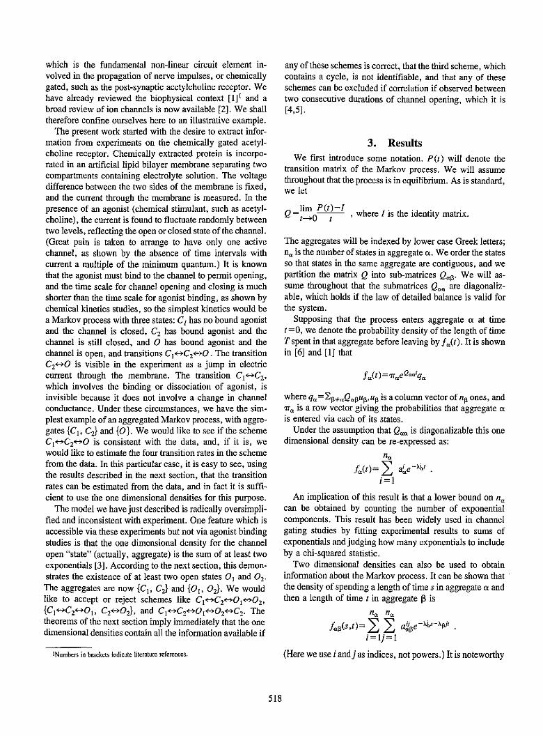
which is the fundamental non-linear circuit element in-volved in the propagation of nerve impulses, or chemicallygated, such as the post-synaptic acetylcholine receptor. Wehave already reviewed the biophysical context [I]' and abroad review of ion channels is now available [2]. We shalltherefore confine ourselves here to an illustrative example.

The present work started with the desire to extract infor-mation from experiments on the chemically gated acetyl-choline receptor. Chemically extracted protein is incorpo-rated in an artificial lipid bilayer membrane separating twocompartments containing electrolyte solution. The voltagedifference between the two sides of the membrane is fixed,and the current through the membrane is measured. In thepresence of an agonist (chemical stimulant, such as acetyl-choline), the current is found to fluctuate randomly betweentwo levels, reflecting the open or closed state of the channel.(Great pain is taken to arrange to have only one activechannel, as shown by the absence of time intervals withcurrent a multiple of the minimum quantum.) It is knownthat the agonist must bind to the channel to permit opening,and the time scale for channel opening and closing is muchshorter than the time scale for agonist binding, as shown bychemical kinetics studies, so the simplest kinetics would bea Markov process with three states: C, has no bound agonistand the channel is closed, C2 has bound agonist and thechannel is still closed, and 0 has bound agonist and thechannel is open, and transitions Cl*C 2 -0. The transitionC2 -0 is visible in the experiment as a jump in electriccurrent through the membrane. The transition C,-C 2 ,which involves the binding or dissociation of agonist, isinvisible because it does not involve a change in channelconductance. Under these circumstances, we have the sim-plest example of an aggregated Markov process, with aggre-gates {Cl, C 2} and {O}. We would like to see if the schemeCl<C 2c0 is consistent with the data, and, if it is, wewould like to estimate the four transition rates in the schemefrom the data. In this particular case, it is easy to see, usingthe results described in the next section, that the transitionrates can be estimated from the data, and in fact it is suffi-cient to use the one dimensional densities for this purpose.

The model we have just described is radically oversimpli-fied and inconsistent with experiment. One feature which isaccessible via these experiments but not via agonist bindingstudies is that the one dimensional density for the channelopen "state" (actually, aggregate) is the sum of at least twoexponentials [3]. According to the next section, this demon-strates the existence of at least two open states O and 02.

The aggregates are now {Cl, C2J and {0, °2}- We wouldlike to accept or reject schemes like Cl-C 2*0 1 *02 ,

{Cl*C2e0 1, C2 02 }, and Cl-C 2 -0 1*0 2 -C2. Thetheorems of the next section imply immediately that the onedimensional densities contain all the information available if

1Numbers in brackets indicate literature references.

any of these schemes is correct, that the third scheme, whichcontains a cycle, is not identifiable, and that any of theseschemes can be excluded if correlation if observed betweentwo consecutive durations of channel opening, which it is[4,5].

3. ResultsWe first introduce some notation. P(t) will denote the

transition matrix of the Markov process. We will assumethroughout that the process is in equilibrium. As is standard,we let

Jim P(t)1IQ=tio t , where I is the identity matrix.

The aggregates will be indexed by lower case Greek letters;n. is the number of states in aggregate a. We order the statesso that states in the same aggregate are contiguous, and wepartition the matrix Q into sub-matrices Q0 p. We will as-sume throughout that the submatrices Q., are diagonaliz-able, which holds if the law of detailed balance is valid forthe system.

Supposing that the process enters aggregate a at timet=0, we denote the probability density of the length of timeT spent in that aggregate before leaving by fe,(t). It is shownin [6] and [1] that

fa(t)= 'rrse Qatq.

where q. =2:p QpuRup is a column vector of nu ones, andTtar is a row vector giving the probabilities that aggregate ais entered via each of its states.

Under the assumption that Q., is diagonalizable this onedimensional density can be re-expressed as:

n.

f,,()= Eta'e-xx,.i=1

An implication of this result is that a lower bound on n.can be obtained by counting the number of exponentialcomponents. This result has been widely used in channelgating studies by fitting experimental results to sums ofexponentials and judging how many exponentials to includeby a chi-squared statistic.

Two dimensional densities can also be used to obtaininformation about the Markov process. It can be shown thatthe density of spending a length of time s in aggregate a andthen a length of time t in aggregate ,3 is

n, n,

Jap5(s~t)=1 Y, a.dge-x&s`Pii=lj=l

(Here we use i and j as indices, not powers. ) it is noteworthy

518

that the same exponential parameters occur in both the oneand two dimensional densities. This might be used to judgethe plausibility of an underlying Markov process model.

The matrix of linear coefficients with ij entry a4,p yieldsinformation about how the aggregates are interconnected:Theorem A. [7] LetAp=p[a$J be the matrix of coefficientsof a two dimensional density above. Then the rank of Act isless than or equal to the rank of QB==pBp say, and AWBdepends on at most pQp(n+npB pp) parameters. The rankof Q<p is less than or equal to the smaller of: the number ofstates in a which are linked directly to states in 13, and thenumber of states in X which are linked directly to states ina. It may be possible to empirically obtain a lower bound onthe complexity of interconnection by fitting two dimen-sional densities and using chi-square tests. We hope to im-plement and test such a procedure in the future.

Higher dimensional densities can be considered also. Thefollowing theorem shows that under certain conditions nomore information about the process can be obtained fromthese densities, however.Theorem B. [7] If, for each aggregate a, the eigenvalues

are distinct and a' *Ofor all i, the higher dimensionaldensities fao ... , (to, . . . 4t), r>l are completely deter-mined by the two-dimensional densities.

Thus, in principle, all the available information about theunderlying process can be extracted from the two dimen-sional densities if the hypotheses of the theorem are satis-fied. By counting the number of independent parametersinvolved in the two dimensional densities, we have thefollowing theorem:Theorem C. [7] Under the assumptions of Theorem B, thefinite dimensional distributions depend on at most L:p~p(n.+np-pcp) parameters. a, B

Thus for example, if there are two aggregates, there isinformation on at most 2p(n,+np-p) parameters. If amodel depends on more than this many parameters, itsparameters are not uniquely identifiable.

Theorem A above suggests one way to study the complex-ity of interconnection between two aggregates. Labarca et.al [5] have also used certain correlation functions for thispurpose. For a particular aggregate a, say, the sequence ofdwell times in that aggregate, T 1 , 2,T.... is a stationary proc-ess, and it can be shown that the covariance function of thatprocess is of the form given in the following theorem:Theorem D. [1] The covariance function is of the form

M-Ir'.(k)= 2, UKilk

i=1

where OicKi<l and k#FO and where M is the rank of thematrix Q. * which is composed of the off-diagonal blockscorresponding to aggregate a in the matrix Q. If M=],r(k) =O for k*O.

The rank of Q, - is less than or equal to the smaller of: thenumber of states in alpha which are linked directly to statesin any other aggregate, and the number of states in otheraggregates which are linked directly to states in a.

Correlation functions can thus be used to obtain informa-tion similar to that in the two dimensional densities as inTheorem A. In the case that there are more than two aggre-gates, the two dimensional densities contain finer informa-tion, however, since a lower bound on the rank of each ofthe matrices Qp which constitute Q. can be obtained.

It is interesting that the covariance function of TheoremD is of the form of the covariance function of a movingaverage-autoregressive process, although the stationaryprocess is distinctly non-Gaussian. It may well be that tech-niques developed for order estimation in the time seriesliterature can be used to estimate M. Labarca et al. [5] wereprimarily interested in testing whether M was greater than 1,which is relatively simple since the large sample distributionof the empirical correlation coefficients in the case M = Ican be used.

4. Further Considerations

We believe that although the results summarized in theprevious section are useful, there are still many open andinteresting questions.

We have developed some necessary conditions for identi-fiability which can sometimes be used to conclude that hy-pothetical models are unidentifiable. It would be useful tohave checkable sufficient conditions as well.

Our analysis applies to stationary Markov processes. Thenonstationary case is of both theoretical and practical inter-est, and we hope to consider that situation in the future.Records from the sodium channel are typically nonstation-ary because of the presence of an absorbing inactivatedstate.

We have only begun to explore practical consequences ofour results for the analysis of experimental data [3]. It istempting to consider estimating the two dimensional distri-butions and basing further analysis on them. Horn andLange [8] have proposed likelihood analysis of sample pathsand Horn and Vandenburg [9] have applied these techniquesto data from the sodium channel. Advantages of their ap-proach are that it is applicable to nonstationary data andmulti-channel data. The likelihood method is computation-ally intensive, however; Horn uses an array processor on aVAX 11/730 and reports that days of computer time arenecessary. An analysis based on the two dimensional distri-butions would be much faster; it is not clear what loss ofstatistical efficiency would be incurred.

Finally, it would be desirable to develop more data-analytic and model-free methods for analyzing experimentalrecords to give qualitative insights that might suggest phys-

519

ical mechanisms. Labarca et al. [3] have used box-plots toadvantage in analyzing data from the chloride channel.

5. References[1] Fredkin, D.R.; M. Montal and J. Rice, Identification of aggregated

Markovian models: application to the nicotinic acetylcholinereceptor. Proceedings of the Berkeley Conference in Honor ofJerry Neyman and Jack Kiefer. Ed. L. Le Cam and R.Olshen, Vol. I, pp 269-290, Wadsworth Publishing Co., Bel-mont, CA (1985).

[21 Hille, B., Ionic Channels of Excitable Membranes, Sinauer Associ-ates, Inc. (Sunderland, MA) (1984).

[3] Labarca, P.; 1. Rice, D.R. Fredkin and M. Montal, Kinetic analysis ofchannel gating: application to the cholinergic receptor channeland the chloride channel from Torpedo californica. Biophys.1 47 469-478. (1985).

[4] Jackson, M.B.; B.S. Wong, C.E. Morris, H. Lecar and C.N. Chris-tian. Successive openings of the same acetylcholine receptorchannel are correlated in their open limes. Biophys. J. 42109-114. (1983).

[5] Labarca, P.; 1. Lindstrom and M. Montal, The acetylcholine receptorchannel from Torpedo californica has two open states. J.Net, rosci. 4 473-496. (1984).

[6] Colquhoun, D., and A.G. Hawkes, On the stochastic properties ofsingle ion channels. Proc. R, Soc. London B 211 205-235(1981).

[7] Fredkin, D.R., and J. Rice, On aggregated Markov processes. Toappear in J. Appl. Prob. (1984).

[8] Horn, R. and K. Lang, Estimating kinetic constants from single chan-nel data. Biophys. J. 43 207-223 (1983).

[9] Hor, R. and Vandenberg, C., Statistical properties of single sodiumchannels. J. Gen., Physiol. 84 505-533 (1984).

520

Journal of Rtsearch of the National Buteau of StandardsVolume 90, Number 6, November-December 1985

Automated Pattern Recognition:Self- Generating Expert Systems for the Future

Thomas L. IsenhourUtah State University, Logan, UT 84322

Accepted: July 1, 1985

Chemometrics and pattern recognition had their start in chemistry in the late 1960's. The most recent review of thearea by Michael DeLaney listed 438 journal articles and books. The three most important areas of future developmentwill be Expert Systems, Relational Data Bases, and Robotics. It should now be possible to combine existing roboticsand artificial intelligence software to create a system which will generate its own expert systems using relational databases. The data will be in the chemical domain and the system I describe we are calling the Analytical Director. TheAnalytical Director will be an artificial intelligence/robotic expert system for the analytical laboratory. The AnalyticalDirector will develop, test, implement and interpret chemical analysis procedures. It will learn from its own experience,the experience of others and communicate what it has learned to others. The Analytical Director will be a self-generatingExpert System. I believe that such systems will, in the future, provide all the advantages of pattern recognition, expertsystems and relational data bases in experimental settings. Problems will continue to be defined by human beings, butmore and more, the laboratory will design, execute and evaluate its own experiments.

Key words: artificial intelligence; chemical analysis; expert systems; pattern recognition; relational data bases; mbotics.

Chemometrics and pattern recognition had their start inchemistry in the late 1960's. Two areas of application ap-peared almost simultaneously, those being learning ma-chines and project dendral, both applied to spectroscopicinterpretation. The former originated in my research groupat the Ugiversity of Washington and have been carried on byus, and my two students, Peter Jurs and Bruce Kowalski,and the latter was developed at the Stanford Artificial Insti-tute by a consortium from Chemistry and Computer Sci-ence. Over the past 15 years a variety of applications haveoccurred which include the following list and probably oth-ers: statistics, modeling and parameter estimation, resolu-tion, calibration, signal processing, image analysis, factoranalysis, pattern recognition, optimization, artificial intelli-

gence, graph theory and structure handling, and librarysearching.

The most recent review of the area by Michael DeLaneylisted 438 journal articles and books. This was an AnalyticalChemistry article which covered the last two years of activ-ity. Clearly, pattern recognition and its applications nowhave an established place in chemistry.

The topic of this presentation is, however, not what hashappened up to the point. Rather it is what will happen in theforseeable future. I believe that the three most importantareas of future development will be expert systems, rela-tional data bases, and robotics. We will talk a little abouteach one of these and then go on to deal in detail with whatmay soon become one of the most, if not the most, sophis-ticated tool that the experimental chemist has ever acquired.

An expert system is, simply stated, a piece of softwarethat behaves like an expert. The origin of expert systemswere instruction manuals that told you what to do basedupon what you encountered in a step by step fashion.

521

About the Author: Thomas L. Isenhour is with UtahState University's Department of Chemistry and Biochem-istry.

Almost everyone is familiar with manuals on "How toFix Your Chevy Station Wagon," etc. These are non-mysterious, and sometimes non-useful, written recipies de-signed to lead you by the hand through a repair, construc-tion, gourmet meal preparation, ecc., that an expert could dobut you could not, at least on your own. Of course, thequality of such systems depends on the knowledge of theexpert, and on the successful transfer of that knowledgefrom that expert to the author and from the author to you.

The modem expert system is usually a computer programthat attempts the same thing, with the same limits of suc-cess. That is, the quality is dependent on the knowledge ofthe expert, the successful transfer of that knowledge fromthat expert to the author and from the author to the user. Itis a little more, however, because the machine can use yourinput to do computations, etc., and while all of this could bedone with a programmed manual, it certainly is faster bycomputer and potentially more accurate. There is lesschance of you failing to follow the directions for correct usethan in a written expert system.

Relational data bases are collections of data that interre-late along traditional and non-traditional lines. In a sense,the relational data base is the social scientist's dream. Givena set of descriptors for each entry, the relational data baseallows very easy cross correlations such as, how many chil-dren in Miami who had braces before the age of 12 also havematernal grandparents alive in Manhattan. Again, a rela-tional data base was always possible with pencil and paper,or even better with three-by-five cards, but it can be greatlyfacilitated in a computer. However, the use is still defined

by the selection of the descriptors and the quality of thequeries.

A robot, according to one handy dictionary, is "a machinedevised to function in place of a human agent." This is quitea broad definition and could refer to an automatic ticketdispenser at a parking garage, an autopilot operating from aninertial guidance system in a jet airplane, or a computerinterfaced with an autoanalyser at a clinical laboratory.

It is my contention that it is now possible to combineexisting robotics and artificial intelligence software to createa system that will generate its own expert systems usingrelational data bases. The data will be in the chemical do-main and the system I describe we are calling the AnalyticalDirector. Simply stated, the Analytical Director will be anartificial intelligence/robotic expert system for the analyticallaboratory. The Analytical Director will develop, test, im-plement, and interpret chemical analysis procedures. It willlearn from its own experience, and that of others, and it willcommunicate what it has learned to others.

The subject of this research is neither automation nor therobot's roll in automation, but rather EXPERT laboratorymanagement working through a combination of robotics andartificial intelligence. We propose to combine robotics andartificial intelligence into an expert system for the analytical

chemistry laboratory. We propose to demonstrate that anAnalytical Director can develop, test, implement, and inter-pret chemical analysis procedures. It is a misconception that

the best use of robots will be exhaustive testing of possiblesolutions to problems. While computationally exhaustivemethods are often quite successful, they are rarely useful toanalytical chemistry. Artificial intelligence is required for areal breakthrough in automated laboratory methodology.

Consider the following analytical problem which mightarise from a relatively simple problem.

Given:10 possible components to a mixture10 reagents10 possible temperatures10 pH values

If each reaction combination were chemically independ-ent, that is, if the results of any combination could belearned by a linear addition of the separate tests, then 10,000procedures could be carried out to determine the entire sys-tem. This might be feasible if, for example, each test couldbe completed in one minute. (This would require just aboutone week of continuous work assuming the robot sufferedno maintenance problems or other delays.)

However, chemical reactions are not usually independ-ent. For example, if one of the components were Fe(ll) andtwo of the reagents were CSN- and citrate ion, there wouldclearly be complex equilibria interactions. If we redo thecalculation considering from I to 10 possible components,

from I to 10 possible reagents and any combination of 10temperatures and 10 pH values, it requires 1.63 x 1015 tests.Again carried out at one minute intervals, assuming therobot could work through the entire set of procedures with-out interruption, 3. lOx 109 years would be needed. Experi-mental design methods might achieve a few orders of mag-nitude improvement but nothing like the 10 orders ofmagnitude necessary to make this approach feasible.

Furthermore, in real analytical situations the number ofvariables and dimensions is often much greater. It is clearthat analytical chemistry cannot be done by exhaustive trialand error. Therefore, if robotics is to have any real effectupon the field an intelligent robot must be created that canchoose meaningful experiments and profit from its experi-ence, as well as the experience of others.

We propose to construct such a system and test it initiallyon a very limited analytical problem to prove chat artificialintelligence can be used to seek efficient paths to complexanalytical problems without resorting to exhaustive trial anderror. To do so our first model system will be very simple,involving 3 ions, 5 reagents, 2 temperatures and 3 pH's.This system can be exhaustively tested with 4320 proce-dures. Assuming I minute tests, 3 days would be required.Exhaustive testing of this model system will produce a set

of observations that will facilitate the development and test-

522

ing of generalized data structures and optimization routinesto be used by the Analytical Director for more complexproblems. For complex problems, the Analytical Directormust develop artificial intelligence methods that circumventthe testing approach.

We have selected a developmental domain that is a closedsystem of simple analytical chemical problems. The domainwill be wet and photometric analysis of simple cations. Theset of manipulative skills required is purposely limited to theabilities of the Zymark system, and the chemical reactionsand spectrophotometric measurements possible limited

to those that can be performed with the available equipment.This way, we plan to be able to test thoroughly the creativecapabilities of the artificial intelligence programs to be de-veloped for the Analytical Director. We have further se-lected the domain of water analysis for an advanced test ofthe Analytical Director. Only by using an unbounded prob-lem will we be able to demonstrate the true capability of theAnalytical Director.

Given a set of standards, reagents, and manipulativeskills, the Analytical Director will develop its own set oftests for each individual cation. These data will be stored ina relational data base keyed on ions, reagents, conditionsand results of spectroscopic measurements. It will be as-sumed initially that no chemistry is known for these ele-ments or reagents. After developing possible individualtests, these tests will be cross compared to identify likelyinterfering reactions. Tests will be characterized by theirquality as defined by time, expense and reproducibility. Asthe best compromise of these components is a value judg-ment, an adjustable value coefficient will be developed.Then possible mixture methods will be systematically testedand compared for success. As this proceeds the relationaldata base will continue to expand. Finally, new unknownswill be introduced into the system to test the ability of theAnalytical Director to adapt to new circumstances. At thispoint literature information will be added to the data base.The Analytical Director will thereby "learn" from the expe-rience of others. Further, the Analytical Director will reportdeveloped procedures for possible use by others.

In summary, the Analytical Director will be a self-generating expert system. I believe that such systems will,in the future, provide all the advantages of pattern recogni-tion, expert systems, and relational databases in experimen-tal settings. Problems will continue to be defined by humanbeings, but more and more the laboratory will design, exe-cute, and evaluate its own experiments.

523

Journal of Research of the National Bureau of StandaidsVolume 90, Number 6, November-December 1985

Regression Analysis of Compartmental Models

T. L. Lai

Columbia University, New York, NY 10027

Accepted: June 24, 1985

Herein we study the problem of assessing, on the basis of noisy and incomplete observations, how muchinformation there is in the data for model identification in compartmental systems. The underlying conceptis that of an "information distance" between competing models, and estimation of this distance on the basisof the given data is discussed. Useful reduction of the dimensionality of the corresponding least squaresproblem is accomplished by regarding the decay rate constants as primary parameters of interest and the otherparameters of the model as nuisance parameters. Estimation of the decay rate function is also discussed.

Key words: compartmental models; decay rate constants; separable least squares problems; system identi-fication.

1. Introduction

Compartmental models are widely used in many fieldsof science and engineering-pharmacokinetics, bio-chemistry, physiology, radioactive isotopes and tracers,to name a few. The basic equations of a typical (linear)compartmental model with k compartments are

k

dxi/dt=ci± 2 (Cix 1 -c1 x9C-cotxy, (1)1= 1,1i'

O<t < , i =, ... , k; where cej are nonnegative constants(called the "turnover rate constants"), compartment 0denotes the environment, and xi =xi(t) is the amount ofmaterial in compartment i at time t. Lettingf%=co andf 7=ciixj for j#AO, fy represents the mass flow rate tocompartment i from compartment j. Under certain as-sumptions (cf. [3], [12])', integration of differential eq (1)leads to

k

x 1(t)=,i + I aye-Z, (2)

About the Author, Paper: T. L. Lai is with theDepartment of Statistics at Columbia. The work hedescribes was supported by the National ScienceFoundation and the National Institutes of Health.

i=l, ..., k; where X,.. . Xk are positive constants(called the "decay rate constants") depending only onthe turnover rate constants cqi, and fi and al are non-negative constants.

Noting that it is often not possible to have accurateand complete measurements from all the compartments,Berman and Schoenfeld [2] considered the degrees offreedom in choosing a compartmental model compatiblewith the data when measurements are incomplete. Inparticular, when one can only measure aggregate input-output kcharacteristics so that one observes only

x(t)= Ixi(t), then one can only identify the rate

constants X,, Xk of the model (2) from the equation

x(t)=B + XA e -X'I=1='

(3)

where B = E 13E and A1 = I a,. In pharmacokinetic ap-

plications, Wagner [10] has shown that many basicquantities of interest can be expressed in terms of theparameters of the reduced model (3), the use of whichhe recommends in lieu of the full model (2) whose spec-ification usually leads to ambiguities in these applica-tions because of noisy and incomplete measurements.

The difficulties in model formulation and identi-fication are compounded when the measurements arenot only incomplete but also are subject to error. Thisleads to the question of assessing, on the basis of noisy

525

' Figures in brackets indicate literature references.

and incomplete observations, how much informationthere is in the data for model identification. If theamount of information is found to be inadequate formeaningful specification of the full model, then it maybe more useful to work with a reduced model or directlywith certain scientifically important characteristics(functions of the parameters) of the model.

Since both eqs (2) (for the individual compartments)and (3) (for the whole system) express the response as apolyexponential function of time t, the statistical prob-lems in the present context are basically those of param-eter estimation for polyexponential regression models.We discuss herein 1) the information content in the datafrom these regression models, and 2) estimation ofmodel parameters and certain functions thereof.

2. Noisy Data and Information Content

Consider the polyexponential regression model

k

yp=13+±ajexp(-Xryti)+fi, i=l, .. 1 n, (4)>=1

where the ej represent random errors. The errors e, areusually assumed to be independent random variableswith zero means. Letting O=(k,, ..., X; a, .a , /3)and

foQt)=j8+aje-'l'+.,.+ake-k'

common models for Var(c) are:

(i) Var(c,) o-' (constant variance error model),(ii) Var(ej) =fo(tQ)o 2 (constant coefficient of

variation model),(iii) Var(Ej)=f0 (1j)a' (Poisson-typeerror model),

Statistical methods for estimating the unknown pa-rameters of the regression function try to "average out"the random errors in various ways. Assuming that ob-servations are taken at equally spaced times t, =( - l)Aand that n=(2k+l)m, the method of Lanczos[6, p. 273] and Cornell [4] uses the sample means

rn-II1=m- y1(r=1..._,2k+1)

to estimate the moving averages , =m i fM(tO) of?=(r- In

the regression function. Replacing p, -Itr- I bY.y,-rin Prony's algebraic equation defining 4,=e`-AmA, solu-tion of the algebraic equation then gives the estimate ofX1. This method therefore tries to average out the ran-dom errors by introducing the new parameters ja, andusing the sample means i. to estimate jw,.

Since the y5 are strongly consistent estimates of Pt' itfollows that the Cornell-Lanczos method is consistent,as was established by Cornell [4]. However, Lanczos [6]gave an example to demonstrate "surprising numericalsnags which may develop on account of the exceedinglynonorthogonal behavior of exponential functions." Thetrue regression function in Lanczos' example is

f0 Q)=0.0951 e<-'+0.8607 e 3 '+1.5576 e-5 1 (5a)

On the basis of 24 successive decay observations in thetime interval (0,1.2] of the form 2.51, 2.04,..., 0.07, 0.06,which are accurate up to 1/2 unit of the second decimal,and assumming knowledge of ,3 0 and k = 3, the pre-ceding method gives the fitted model

foQ)=0+0305 e-'5 an2202 e ani (5b)

Although the true parameters are disappointingly farfrom their estimates, the fitted function (5b) is remark-ably close to the true function (5a), and one cannotdistinguish between the two models within the errors ofthe measurements.

An alternative method to estimate the unknown pa-rameters is that of least squares. The estimate 6 of 8 isthe value of '} that minimizes

S()=I wily, -t0ff, (6)

where the w, are suitably chosen weights. Note that

2Xw1Ef0 (ti) -f,(ti)]. (7)

Moreover, if the weights wi are so chosen that wi Var (e,)are bounded, then

a

YwJfor(ti) -A(tjA]1 =

0(T:wj~f0(ti)-Ar(tj)h w.p. 1 (8)

(with probability 1) as

(9)

The quantity d(6,y)(=E{S(y)-S(O)}) defined in (9) isa measure of the separation (distance) between v and theparameter vector 0 reflected by the data. When the Eare normal N(0,l1/wj) random variables, 1/2 d(0,y) isthe Kullback-Leibler information number and the leastsquares estimate coincides with the maximum

526

d (Oy) = Twi [f,(tj -fo(ii)1'- �.

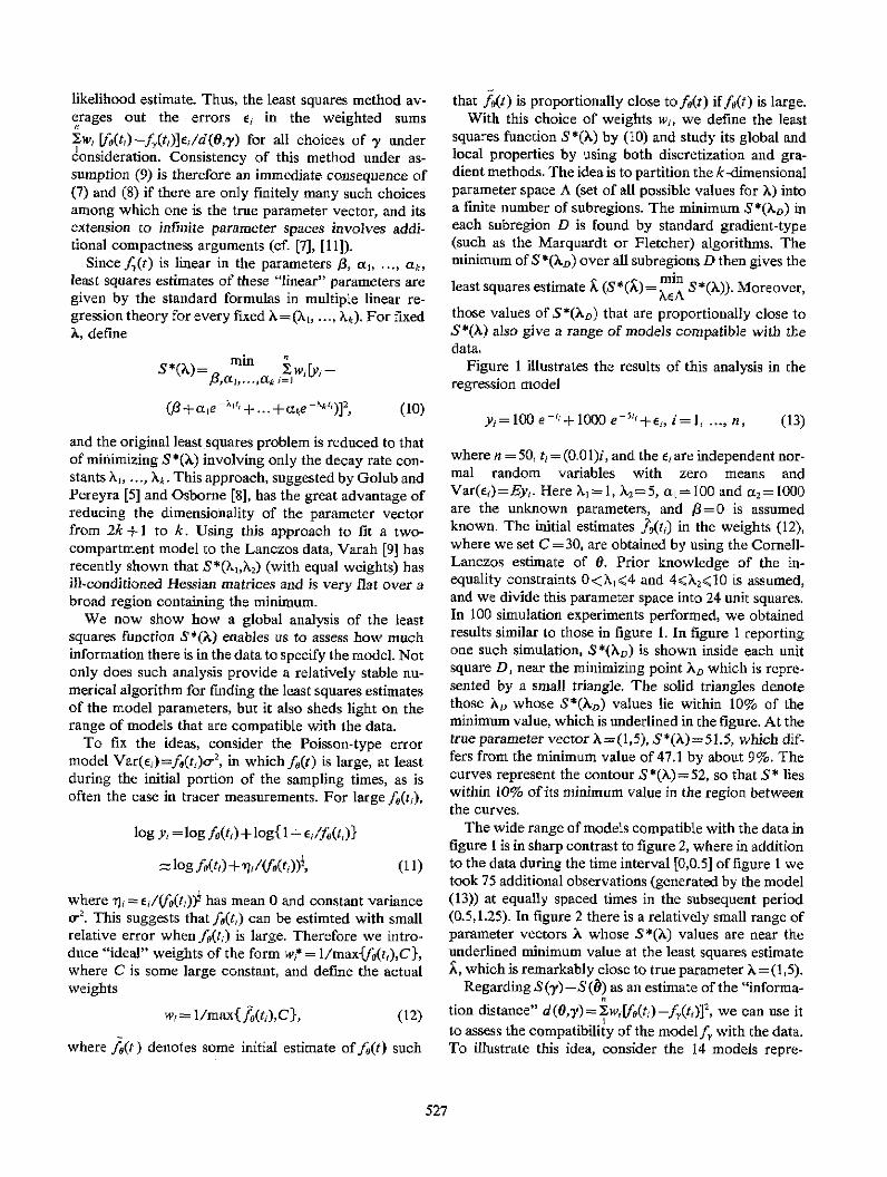
likelihood estimate. Thus, the least squares method av-erages out the errors ei in the weighted sums

1w1 [f0(t,)-f(j)]c,/d(0,y) for all choices of y underconsideration. Consistency of this method under as-sumption (9) is therefore an immediate consequence of(7) and (8) if there are only finitely many such choicesamong which one is the true parameter vector, and itsextension to infinite parameter spaces involves addi-tional compactness arguments (c£f [7], [111).

Since fQ) is linear in the parameters ,3, a, ... , ak,

least squares estimates of these "linear" parameters aregiven by the standard formulas in multiple linear re-gression theory for every fixed X=(X,, .. , Xk). For fixedA, define

min2w, kj[V -

'=1l- j

(+ ale '' +...+ae )]' (10)

and the original least squares problem is reduced to thatof minimizing S *(A.) involving only the decay rate con-stants X,.., A. This approach, suggested by Golub andPereyra [5] and Osborne [8], has the great advantage ofreducing the dimensionality of the parameter vectorfrom 2k +I to k. Using this approach to fit a two-compartment model to the Lanczos data, Varah [9] hasrecently shown that S*(X,,X2) (with equal weights) hasill-conditioned Hessian matrices and is very flat over abroad region containing the minimum.

We now show how a global analysis of the leastsquares function S*(X) enables us to assess how muchinformation there is in the data to specify the model. Notonly does such analysis provide a relatively stable nu-merical algorithm for finding the least squares estimatesof the model parameters, but it also sheds light on therange of models that are compatible with the data.

To fix the ideas, consider the Poisson-type errormodel Var(e. =f0 (t,)ar2 , in whichf 0 (t) is large, at leastduring the initial portion of the sampling times, as isoften the case in tracer measurements. For large f0 (tj),

log yj =log f0t6+log{l + Ecf6 (t)}

= log MO(ti) + 71{/VVO(0 ))', (1 1)

where rj = c,(f6t?))2 has mean 0 and constant varianceit. This suggests that fo(t,) can be estimted with smallrelative error when f0 (tj) is large. Therefore we intro-duce "ideal" weights of the form w* = I/max{(tj),C},where C is some large constant, and define the actualweights

w1= l/maX{fa(tj),C}, (12)

where fo(t ) denotes some initial estimate of fA(t) such

that foQ) is proportionally close to ft) if f(t) is large.With this choice of weights wi, we define the least

squares function S*(L) by (10) and study its global andlocal properties by using both discretization and gra-dient methods. The idea is to partition the k-dimensionalparameter space A (set of all possible values for X) intoa finite number of subregions. The minimum S*(XD) ineach subregion D is found by standard gradient-type(such as the Marquardt or Fletcher) algorithms. Theminimum of S *(X) over all subregions D then gives the

least squares estimate A (5*(S2=V1 5*(A)). Moreover,

those values of S*(Xn) that are proportionally close toS*(A) also give a range of models compatible with thedata,

Figure I illustrates the results of this analysis in theregression model

yj-= 100 e+" 1000 e 5 "'+e1 , i=1, ..., n, (13)

where n =50, tj=(0.0l)i, and the Ei are independent nor-mal random variables with zero means andVar(cj)=Ey,. Here X,1=1, At2=5, a,=100 and a2= 1000are the unknown parameters, and /3=0 is assumedknown. The initial estimates 79(t1 ) in the weights (12),where we set C=30, are obtained by using the Cornell-Lanczos estimate of 0. Prior knowledge of the in-equality constraints O<X,<4 and 4cX2<10 is assumed,and we divide this parameter space into 24 unit squares.In 100 simulation experiments performed, we obtainedresults similar to those in figure 1. In figure 1 reportingone such simulation, S*(XD) is shown inside each unitsquare D, near the minimizing point XA which is repre-sented by a small triangle. The solid triangles denotethose X, whose S*(X. ) values lie within 10% of theminimum value, which is underlined in the figure. At thetrue parameter vector X=(1,5), S*(A)=51.5, which dif-fers from the minimum value of 47.1 by about 9%. Thecurves represent the contour S*(X)=52, so that S lieswithin 10% of its minimum value in the region betweenthe curves.

The wide range of models compatible with the data infigure I is in sharp contrast to figure 2, where in additionto the data during the time interval [0,0.5] of figure I wetook 75 additional observations (generated by the model(13)) at equally spaced times in the subsequent period(0.5,1.25). In figure 2 there is a relatively small range ofparameter vectors A whose S*(AL) values are near theunderlined minimum value at the least squares estimateI , which is remarkably close to true parameter At=(I,5).

Regarding S(y)-S(0) as an estimate of the "informa-tion distance" d(0,y)=Iw,"Ve(tj)-f,(t,)] 2 , we can use itto assess the compatibility of the modelf, with the data.To illustrate this idea, consider the 14 models repre-

527

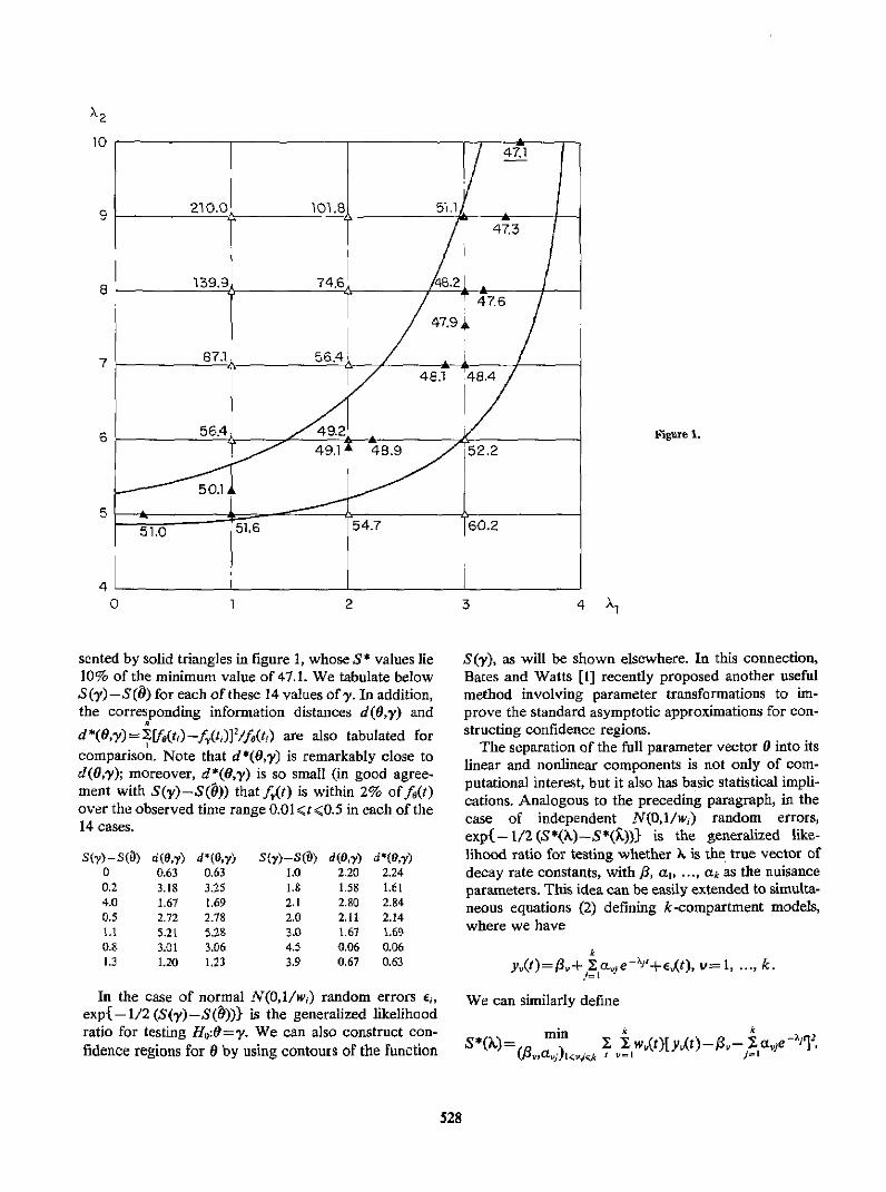
X2

10 -___________ ________________101.8

9. 2l0.0 101.6

8- 13931 74.6

7 871 56.448

6 5.

0 1 2

sented by solid triangles in figure 1, whose 5* values lie10% of the minimum value of 47.1. We tabulate belowS(y)-S(O) for each of these 14 values of y. In addition,the corresponding information distances d(O,y) and

d*(Oy)=Z&(tf)-f,(rj)]1fo(tj) are also tabulated forcomparison. Note that d4*(O,y) is remarkably close tod(O,y); moreover, d*(Oy) is so small (in good agree-ment with 5(y)-S(0)) that f,(t) is within 2% offo(t)over the observed time range 0.01r<0.5 in each of the14 cases.

S(m)-S(O)00.24.00.51.10.81.3

d(O,y)0.633.181.672.725.2t3.011.20

d*O6,y)0.633.251.692.785.283.061.23

S(y)-S(D)1.01.82.12.03.04.53.9

d(O,y)2.201.582.80

d(O,-y)2.241.612.84

2.11 2.14\t61 1.69

0.06 0.060.67 0.63

In the case of normal N(0,l1/w) random errors ej,exp{- 1/2 (S(y)-S(&))} is the generalized likelihoodratio for testing Hi:O=y. We can also construct con-fidence regions for 0 by using contours of the function

Figure 1.52.2

60.2

3 4 A1

5(y), as will be shown elsewhere. In this connection,Bates and Watts [I] recently proposed another usefulmethod involving parameter transformations to im-prove the standard asymptotic approximations for con-structing confidence regions.

The separation of the full parameter vector 0 into itslinear and nonlinear components is not only of com-putational interest, but it also has basic statistical impli-cations. Analogous to the preceding paragraph, in thecase of independent N(O,l/w,) random errors,exp(-1/2(S*(X)-4S(;Q))} is the generalized like-lihood ratio for testing whether X is the true vector ofdecay rate constants, with j3, a,, -.. , ak as the nuisanceparameters. This idea can be easily extended to simulta-neous equations (2) defining k-compartment models,where we have

y~t)=: + !¾e aje-Y'+ct), v= 1, k./=1

We can similarly define

SYRIA)= mn k w()yt-1vXLv lMl ' 2=1

528

>'2

9

8

7

Figure 2. 6

5

40

and interpret exp{-1/2(S*(Q)-S*(X))}alized likelihood ratio for testing whethervector of decay rate constants on the basisall k compartments.

2

as a gener-X is the trueof data from

3. Decay Rates and Their Estimation

Consider the polyexponential regression model (4).As illustrated in figure 1, one often encounters a widerange of rate parameter vectors (X,, ..., 4L) that arecompatible with one's data. In such circumstances, sincethere is not enough information to estimate the individ-ual rate constants, it is more meaningful to considerthem in a combined characteristic, such as the fractionalrate of decay

r(t)=lim 8-'{l-f 0(t+8)/f 0(t)}=-(d/dt) logfo(t)

at different time points t of interest. Letting XO=0 and

a0 =/3, the logarithmic derivative of fo(t)= aj e i isgiven by - I times 10

3 4 Xi

k kr(t)= Y p,(t)X1, wherep 1(t)=aje-'Xiu/Za e -'.

i=0 = (14)

Thus, r(t) is a convex combination of the rate constantsXi, with the proportional size of the 1th exponential termas the natural weighting factor for the decay rate A,.

To estimate r(r) at a particular time point r within therange of sampling times, we propose to balance "globalinformation" from all sampling times (leading toweighted least squares estimates described in sec. 2)with "local information" from only the sampling timesnear 7. We start by using the method of section 2 on allthe data to find a region A0 of rate parameters (XA, . .., Xk)that are compatible with the data. To choose a vector inA, that will provide the best estimate of r(i-), we notethat the logarithmic derivative - r(r) is a "local" quan-tity involving only sampling times near r, and it is there-fore reasonable to weight the observations not only bytheir variability but also by how far their sampling timesare from i, putting more weight on sampling times near7. With this new set of weights w,(T), we calculate the(constrained) least squares estimate 8(r) of the parame-ter vector 0, under the constraints XcA0 and aj>0(i=0,1, ..., k). Substituting the unknown parameters in eq (14)

529

'L281.5

1584.7A 346.8 212,4

5.287.6

924.7 242.9 168.5304.2

s38.31 X Be, a:. 2 335.3

249.4 141.8

16 130.7 228153.6 385.9

3. L1 30.513010.7 2284 1.

I

by these least squares estimates, we obtain the estimate?(r) of r(r).

A detailed discussion of the procedure sketchedabove, together with a comparative study of this ap-proach and the popular curve-peeling methods for com-partmental analysis (cf. [12]), will be presented else-where.

The author thanks Dr. Hung Chen for helpful dis-cussions.

References

[I] Bates. D. M., and D. G. Warts, Parameter transformations forimproved approximate confidence regions in nonlinear leastsquares Ann. Statist. 9, 1151 (1981),

[21 Berman, M., and R. Schoenfeld, Invariants in experimental dataon linear kinetics and the formulation of models. J. Appl.Phys. 27, 1361 (1956).

[3] Coddington, E. A., and N. Levinson, Theory of Ordinary Dif-ferential Equations. McGraw-Hill, New York (1955).

[41 Cornell, R. G. A method for fitting linear combinations of ex-ponentials. Biometrics 18, 104 (1962).

[5] Golub, G. H., and V. Pereyra, The differentiation of pseudo-inverses and nonlinear least squares problems whose vari-ables separate. SIAM J. Numer. Anal, 10, 4L3 (1973).

[6] Lanczos, C, Applied Analysis. Prentice Hall, Englewood Cliffs(1956)

[71 Ljung, L., Consistency of the least squares identificationmethod. IEEE Trans. Autom. Contr AC-21, 779 (1976).

[51 Osborne, M R., Some special nonlinear least squares problems.SIAM J. Numer. Anal. 12, 571 (1975).

[9] Varah, J. M., On fitting exponentials by nonlinear least squares.SIAM J. Sci. Stat. Comput. 6, 30 (1955),

[101 Wagner, J. G., Linear pharmacokinetic equations allowing di-rect calculation of many needed pharmncokinetic parametersfrom the coefficients and exponents of polyexponential equa-lions which have been fited to data. J. Pharmacokin. fiop-harm. 4, 443 (1976).

[II Wu, C F., Asymptotic theory of nonlinear Least squares esti-mation. Ann, Statist. 9, 501 (1981).

[12] Zeirler, K., A critique of compartmental analysis. Ann. Rev.Biophys. Bioeng. 10, 531 (1981).

DISCUSSIONof the T. L. Lai paper,Regression Analysis of Compartmental Models

T.-H. Peng

Oak Ridge National Laboratory

One of the major tasks of marine geochemists is deter-mining the uptake by the sea of CO2 derived from thecombustion of fossil fuels. Until valid models of thegeneral circulation of the ocean are constructed, thistask will have to be done with box models calibratedthrough use of the distribution of natural radioisotopesand transient tracers.

We need to explore how sensitive the uptake of fossilfuel CO2 is to the basic design of these models and howthe design can be improved by simultaneously fitting thedistributions of several tracers. Five different 11-boxthermocline circulation models of the temperate NorthAtlantic were constructed for this purpose.* Anthro-pogenic tritium, 3He, and radiocarbon are used as trac-ers to calibrate these models. The temporal input func-tions of these tracers differ considerably from oneanother. So also do the geographic patterns of theirinputs and their geochemistries in the sea.

Using the basic equation of the box model [e.g., eq (1)of T.L. Lai's presentation at this conference] and the

finite difference method of computation for mass bal-

ance in each box, these thermocline ventilation modelswith differing circulation patterns were calibrated toyield a tritium distribution similar to that observed dur-ing the Geochemical Ocean Section Studies(GEOSECS) survey in 1973. These models were thenrun for 'He and bomb-produced 4C. While the modelsdiffer significantly in their ability to match the observed3He and 14C distributions, these differences are not largeenough to clearly single out one model as superior. Thisinsensitivity of tracer to tracer ratio to model design isreflected by the nearly identical uptake of CO, by thevarious models. This result also suggests that the uptakeof CO2 by the sea is limited more by the rates of physicalmixing within the sea than by the rate of gas exchangeacross the sea surface.

- Research of the application of box models for the geochemicalmodeling of oceans was supported jointly by the National ScienceFoundation's Ecosystems Studies Program under Interagency Agree-ment DEB 8115316 and the Carbon Dioxide Research Division, Of-

Eice of Energy Research, U.S. Department of Energy, under contractDE-ACO5-840R21400 with Martin Marietta Energy Systems, Inc.

530

Journal of Research of the National Bureau of StandardsVolume 90, Number 6, November-December, 1985

Measurement and Controlof Information Content

in Electrochemical Experiments

Sam P. Perone and Cheryl L. HamLawrence Livermore National Laboratory, Livermore, CA 94550

Accepted: July 1, 1985One of the most important problems in chemical analysis is the interpretation of analytical data. The difficulty of this

task has been further compounded by the data explosion. Chemical information relevant to the particular analysis

problem is hidden within excessive amounts of data, This problem could be alleviated through knowledge and control

of the information content of the data. Information theory provides a means for the definition, evaluation, andmanipulation of quantitative information content measurements. This paper provides a general review of some of the

basic concepts in information theory, including history, terminology, entropy, and other information content measures.The application of information theory to chemical problems requires some modifications. The analyst is usually only

interested in a subset of the information (data) which has been collected. Also, this relevant chemical information is

dependent upon not only the informational goals of the problem, but the completely specified procedure as well. This

paper reviews chemical applications of information theory which have been reported in the literature including applica-

tions to qualitative analysis, quantitative analysis, structural analysis, and analytical techniques. Measures of informa-

tion and information content and figures of merit for performance evaluations are discussed. The paper concludes witha detailed discussion of the application of information theory to electrochemical experiments and the empirical determi-

nation of the information content of electroanalytical data.

Key words: chemical analysis; chemical information; data explosion; electrochemical experiments; informationcontent measurements; information theory, chemical applications

Introduction

Data interpretation is one of the most challenging prob-lems of chemical analysis. Both the data-rich and the data-

limited cases stress the need for efficient methods to extract

chemical information from the available data. Data-rich

analyses result from the ability of modem chemical instru-

mentation to generate enormous amounts of data in short

periods of time. The current trend towards more exotic

About the Authors, Paper: Sam P. Perone and CherylL. Ham are with Lawrence Livermore's Chemistry & Mate-

rials Science Department. The work they describe was sup-

ported by the Office of Naval Research apd the Lawrence

Livermore National Laboratory

hybrid instruments buries the chemical information evendeeper within the data. Alternatively, data-limited analysesoften result from limitations in appropriate sensors, accessi-ble techniques, time, and manpower. The need for efficient

methods to extract chemical information is superseded onlyby the need to acquire information-rich data.

Improving accessibility of chemical information empha-sizes the importance of good experimental design and re-

quires a re-evaluation of the traditional approach to chemi-cal analysis. The typical approach involves using

foreknowledge about the samples to choose an anlytical

procedure. The analytical procedure, which may involvemore than one analytical technique, is used to produce asmuch data as possible which is collected for later analysis.Data interpretation is performed by the analyst using asmuch intuition and background knowledge as possible. In

531

the data-rich case, emphasis is often on data reduction. Thedata-limited case emphasizes information extraction.

A more efficient and desirable approach to chemical anal-ysis would be to maximize the amount of information ob-tained relevant to the current problem, while minimizing theamount of analytical effort, time, and collected data, Theevaluation, selection, and optimization of analytical proce-dures need to be investigated further, In order to study thisproblem, a method for the quantification of chemical infor-mation must be defined. This paper reviews some relevantinformation theory concepts and describes applications tochemical analysis. Illustrations have been taken from theliterature, as well as from our own recent work, to demon-strate the value of applied information theory for optimizedchemical analysis methods.

Information Theory Concepts

Information theory [1-4]1 is concerned with the study of

information and its transmission. The earliest information

theorists studied the encoding and decoding of secret codes.Modem work on information theory can be traced back tothe 1920's beginning with Carson's study of frequency

modulation. Nyquist determined the minimum bandwidthrequired for the transmission of a definite quantity of infor-mation. Hartley established a definite bandwidth-timeproduct required for the tranmission of a definite quantity of

information. However, most of the present work in informa-tion theory is based upon probablistic models of communi-cation developed by C.E. Shannon in 1948 [5]. Simply

stated, the basic principle is that a message with a highprobability of random occurrence conveys little informa-don. The most information is conveyed by the message that

is least likely to spontaneously occur.This principle is formalized by the concept of entropy

which equates information and uncertainty. Entropy is aquantitative measure of the amount of information suppliedby a probabilistic experiment. It is based upon classicalBoltzmann entropy from statistical physics. Shannon's for-mula, eq (1) defines the entropy or the average information

N

HaV=Iav= P(xi) log2 p(xi) , (1)

to be equal to the weighted average of the specific informa-tion for each event in the system under consideration.Specific information [61 is information conveyed by theoccurrence of a particular event and is quantified by the-log 2 of the probability of the event (p(xj)). Entropy islimited by a maximum of log2 N (Hartley's equation), where

Figurcs in brackets indicate literature references.

N is the number of events, when considering a set of mutu-ally exclusive but equally probable events [1,6,7]. For ex-ample, consider the measurement of three distinguishableintensity levels. If the probabilities of measuring these lev-els are 0.25, 0.30, and 0.45, respectively, the averge en-tropy would equal 1.5 bits. The amount of specific informa-tion conveyed by the measurement of each level wouldequal 2.0, 1.7, and 1.1 bits, respectively. Notice that theleast likely level to be measured does indeed convey themost information. The maximum entropy is equal to 1,6bits. A thorough treatment of the mathematical basis ofentropy and its properties is given in a book by Mathai and

Rathie [21.Redundancy [6] is the difference between the maximum

information and the average information eq (2). Relative

N

Id =10g2 N - p(xi) log2 p((x) (2)

redundance is the ratio of the redundance to the maximuminformation [6]. Relative information content is the ratio ofthe actual average information to the maximum information[11. Redundancy can then be expressed as the remainingfraction not due to relative information [1]. In the aboveexample there is 0.1 bit of redundancy and 0.062 relativeredundance. If the actual average information is equal to 1.4bits, the relative information content is equal to 0.88 and theredundancy equals 0.12.

Types of Information

The concept of information as used in information theoryrefers to the choice or uncertainty of outcomes when regard-ing distinguishable elements with respect to some randommechanism. Information is a system based upon elementsthat have been agreed upon for the representation of infor-mation (characters) and the relationships between them(codes). It is not a measure of meaning as used in the usual

sense, which implies a subjective evaluation. The conceptof information as used in chemical analysis encompasses theuncertainty regarding the quantity, identity, chemical struc-ture, or properties of the analyte of interest.

Preinformation or foreknowledge [1] is the prior knowl-edge concerning the occurrence of events. The informationconveyed by the occurrence of more than one independentevent is simply the sum of the information conveyed by eachevent individually. However, if the occurrence of a second

event is dependent upon the occurrence of the first event, theforeknowledge of the first event reduces the amount of in-formation conveyed by the second event. Therefore, theamount of information conveyed by a series of events withinthe system under consideration is always less than or equal

532

to the sum of the information conveyed by each of the eventsseparately.

Preinformation is probably the most commonly used in-formation theory concept in chemical analysis. Chemicalpreinformation [8] is information that is known prior toperforming the current analysis. It may result from experi-ence, preliminary analyses, etc. It is used to reduce theeffort required to solve the analytical problem. Preinforma-tion may be quantified through the use of entropy-basedmeasures [8]. The uncertainty before the analysis for a dis-crete variable, such as chemical identity, is quantified by theuse of the a priori probabilities for identification in Shan-non's equation (eq 1). The uncertainty for a continuousvariable such as concentration or signal intensity is ex-pressed by integrating the a priori probability density func-tion over the range of interest eq. (3).

H(X)=-f p(x) 10g2 P(x) d (3)xI

Joint information [I] is information that is provided bymore than one event. It can be quantified by substituting thejoint probability of occurrence for the events into Shannon'sequation (eq 1). In the case of independent events, the jointprobability of occurrence is simply the product of the apriori probabilities of occurrence. For nonindependentevents, it is the product of the a priori probability for thefirst event with the conditional probabilities for the other

events.Mutual information describes the amount of information

in one event that determines the state of another event. Itmay also be thought of as the average amount of informationrequired to distinguish members of different classes, Isen-hour et al. [9] investigated the relationship between mutualinformation and classification in the determination of chem-ical functionality for 200 compounds based upon binaryencoded (peakino peak) infrared spectra. Mutual informa-tion was calculated as the difference between the total aver-age entropy and the average conditional entropy. The totalaverage entropy is the average amount of information re-quired to distinguish between the 200 spectra under consid-eration. It is calculated as a weighted average of the proba-bility of occurrence of a peak maximum for each spectralinterval using Shannon's formula (eq 1). The average condi-tional entropy is the average amount of information requiredto distinguish between members of the same class. Averageconditional entropy is calculated as the sum of the classconditional entropies weighted by class size. In the case oftwo separable, equally probable classes, the independentmutual information is equal to one bit. A value for mutualinformation greater than one bit implies the inclusion ofredundant information in the data. The square root of mutual

information was shown to be linearly related to the maxi-mum likelihood classification ability.

Figures of Merit

The application of information theory concepts to chem-istry is most familiar in the evaluation of analytical methods.Figures of merit such as accuracy, precision, and detectionlimit have long been used to evaluate the attainment ofinformational goals such as concentration, resolution, andsensitivity, respectively. Figures of merit are measures ofgoal achievement for completely specified procedures thatcan be used for evaluating, selecting, and comparing analyt-ical procedures. Other quantifiable factors that can be usedto determine the applicability of analytical procedures to aparticular problem include sensitivity, selectivity, speed ofanalysis, personnel requirements, and cost of the analyticalprocedure.

Grys [10] described five new functional concepts: accu-racy, limit of detection, firmness, efficiency, and cost,which result in judgements of acceptibility of analyticalmethods. Accuracy is expressed in terms of recovery andreproducibility. The contribution due to recovery can becalculated by summing the percentage of different lossesthroughout the whole procedure. Reproducibility is ex-pressed by the ratio of the full range to 100 times the idealrange.

Limit of detection is the concentration of a sample thatgives a reading that is equal to twice the confidence half-interval for a series of ten determinations of the blank testvalue determined to 99% certainty. It is measured in mg perkg, or ppm, and is given by multiplying the standard devi-ation by 2.17, a factor that is determined from the t test fort0 01 and n = 10.

Firmness is an index of the effects of different factorsupon the results. It is equal to the total deviation fromexpected values caused by the presence of equimolaramounts of interfering substances or connected with 5%changes in optimum reaction conditions such as acidity orreagent concentrations.

Efficiency provides information about the time consump-tion during the course of the whole procedure. It is ex-pressed as the time of effective labor for one sample inminutes divided by 100.

Cost is a measure of the expenditure of materials andequipment used for the analysis of one sample by a newmethod in relation to the least expensive method. The costof any desired method by which the analysis can be per-formed may be substituted for that of the least expensivemethod. It is given by dividing the ratio of the cost of thenew method to the old method by 1000.

Eckschlager [11] discussed two informational variables,time-information performance and specific price of informa-

533

don, which can be utilized in the evaluation and optimiza-tion of analytical methods. Time-information performance[12] can be rewritten as the ratio of information content tothe time required for the analysis, including the analysisitself plus the time required to prepare the equipment for theanalysis of the next sample. The time required for analysiscan be partitioned into two segments, the basis time and the

time required for the performance of N parallel determina-tions. The specific price of the information [11] is definedas the ratio of the cost of the analysis to the amount ofinformation obtained through simultaneous determination ofN components.

Danzer and Eckschlager [13] defined a general measureof information efficiency as the product of efficiency coeffi-cients that are based upon the ratio of the value of thevariable characterizing the properties required for the solu-tion of particular analytical assignments to the actual valuethat the method provides. A ratio greater than one impliesthat more of the property is required than is provided by themethod and the efficiency coefficient is assigned the valueof zero. Otherwise, the efficiency coefficient is assigned thevalue of the ratio. They also defined a measure of infornia-tion profitability as the ratio of the information efficiency tothe specific price of the information. Results for the deterni-nation of manganese in low-alloy steels were tabulated forseven analytical methods: titrimetry, potentiometric titra-tion, photometry, atomic absorption spectrophotometry, op-tical emission spectroscopy, optical emission spectrogra-phy, and optical emission spectrometry. The resultsdemonstrated that information efficiency and informationprofitability are not always correlated. For example, al-though potentiometric titration has almost five times theinformation efficiency of titrimetry, both methods have thesame information profitability when the duration of the anal-ysis should be less than one day.

Informing Power

Informing power is a measure of the amount of informa-tion available in a given analytical procedure. The conceptwas developed by Kaiser [14] with respect to spectrochem-ical methods of analysis eq (4) as a function of the resolving

Pimf= | R(v) log2 S (v) - (4)fV. ~~~V

power, R(v), the maximal number of discernable steps forthe amplitude, S(v), and the spectral range, v. to Vb. If theresolving power and the maximal number of steps are fairlyconstant over the spectral range under consideration, in-forming power reduces to eq (5). For example, a grating

Pinf=Rav logo SV, In (vbdv) (5)

spectrograph system with a resolving power of 2X 105, aspectral range from 2000 to 8000 A, and 100 discernablesteps in measured intensity levels at each wavelength wouldhave an informing power of 2x 106 bits. It is obvious thathere the resolving power is the most important factor inmaximizing informing power. In the case of a nondisper-sive, monochromatic method, resolving power betweenpeaks at different wavelengths is not applicable and inform-ing power is simply the log2 of the number of discemableamplitude steps at that wavelength. For example, 100 dis-cernable intensity steps yields an informing power of 7 bits.The informing power for the corresponding polychromaticmethod is that for the monochromatic method multiplied bythe number of frequencies. If the number of steps is differentfor each of the different frequencies, then the informingpower is the same as for a collection of monochromaticmethods, and the log2 of the number of steps is summedover each of the different frequencies

Fitzgerald and Winefordrer [15] extended the applicationof informing power to time-resolved spectrometric systemswith the addition of a second resolving parameter, R,. Ifboth resolving powers and number of discemable steps arenearly constant over the range, then informing power re-duces to eq (5) multiplied by R. In (t21t1 ). For example, anatomic fluorescence spectrometer with an average resolvingpower of 3000 over a spectral range from 200 to 500 nm

;with an averge of 200 discernable intensity steps has aninforming power of 5.7x 104 bits. The informing power isincreased to 9.7x Ihibits for a range of 10-9 (tj) to 10-6 sewith a measurement time limited by the lifetimes of theexcited species of 10' sec (t2) and a 8! of 10- 9 sec (R.equals (t2 -,t)/Br). Comparisons of the inforning power fora single beam molecular absorption spectrophotometer, nor-mal molecular absorption phosphorimetry and time-resolved phosphorimetry showed an increase in the inform-ing power by a factor of two for the normal phosphorimeterover the spectrophotometer. The addition of a time resolu-tion element to phosphorimetry increased informing powerby a factor of 450. The addition of a time resolution elementto atomic fluorescence spectrometry increased the informingpower by a factor of 170. Informing power was also used tocompare analytical methods as well as to compare analyticalinstruments. A general photon counter was shown to havean informing power three times larger than that for an analogsynchronous detection system.

Yost extended the application of informing power totandem mass spectrometry [16,17], a method capable ofgenerating enormous amounts of data. In the case of aquadrupole mass filter, the minimum resolution element, bxis constant rather than the resolving power, R (x). Informingpower can then be calculated as shown in eq (6). A quad-

534

P.f F -1092 S ( Xb )l-Xa I (6)ax

rupole mass spectrometer with unit mass resolution, a massrange of 1000, and an ion intensity range of 212 bits wouldhave an informing power of 1 .2X 104 bits. The addition ofanother resolution element produces a double integral in theinforming power equation that is equivalent to the theproduct of the informing power of the two elements. Theaddition of a capillary gas chromatograph with a nearlyconstant 105 theoretical plate resolution over a one houranalysis time, results in 6.6X 106 bits of informing power.The addition of a second quadrupole mass spectrometer withthe same characteristics results in 1.2 x 107 bits of informingpower. The combination of a capillary gc/ms/ms systemresults in an informing power of 6.6X 109 bits, an increaseby a factor of 5.5 X 105 over the original quadrupole massspectrometer. The effect of experimental parameters on in-forming power was also demonstrated by Yost [16,17]. Thevariables associated with the collisionally activated dissoci-ation process are potential resolution elements. Energy- andpressure- resolved ms/ms has an informing power of3.6x 109 bits.

The informing power metric can also be applied to elec-trochemistry. Using a current range of -20 to +20 1iA thatcan be measured to within .005 IiA yields 4X 103 discem-able steps. Eq (6) can be used to calculate the informingpower for a cyclic staircase voltammetry (CSCV) experi-ment in which each current pulse is sampled and analyzed.An experiment with a staircase step of 13.5 mV (8x) and apotential range scanned from 0.0 to -1.73 V yields3.1 x 103 bits of information.

Boudreau and Perone [18] demonstrated quantitative res-olution in programmed potential step voltammetry for over-lapped peaks with 30 mV separation between half wavepotentials. If only resolved peaks are analyzed and thesmallest resolution is 30 mV, the informing power is1.4x 103 bits. The addition of a time resolution elementincreases the informing power for electrochemical methods.Taking 45 equally spaced current measurements on eachstep at a sweep rate of 1.00 V/sec for the CSCV experimentincreases the amount of information to 3.5x 107 bits. Theamount of information obtained from CSCV experimentscan be easily manipulated by changing or adding resolutionparameters.

Informing power can be used as a figure of merit for acompletely specified method or system. Although the in-forming power of instrumental techniques may seem exces-sive when compared to the maximum information as calcu-lated by Hartley's formula, it must be remembered thatinforming power is simply a measure of the maximal num-ber of bits of information available in the procedure, notnecessarily the useable or necessary amount of information.

Limitations in informing power arise from differences be-tween practical and calculated resolving power. The lack ofindependence between the bits of information, noise, andinterference result in the reduction of the useful informingpower. Informing power can be partitioned into the amountof information required for the solution of the problem andthe amount of redundant information required to provide agiven level of confidence.

Information Content

One of the most important concepts in information theoryis that of informational gain or information content [19].This is equal to the change in entropy due to the experi-ment and is quantified by the difference between the en-tropy using a priori probabilities and the entropy using aposteriori probabilities eq (7). The use of Shannon's

I(X 1Y)=H(X)-H(XIY) (7)

formula eq (1) to calculate the entropy does not guarantee anon-negative information content. However, another infor-mational measure eq (8) always results in non-negative

N

I(XIy)=- p(X1Iy) 1lg2 [P(XiJY)Ip(XX)]i

(8)

values. For equal a priori probabilities, information contentas calculated by Eqs (7,8) are equivalent. Since informationcontent as discussed above can only be established after theanalysis, these measures cannot be used as a quality crite-rion for selecting an analytical procedure. However, theycan be used to evaluate the performance of a procedure.

Measures of information content has been applied to in-formation theory models of structural analysis, qualitativeanalysis, quantitative analysis, trace analysis and instrumen-tal analysis. Eckschlager and Stepanek have published abook [7] and a review article [8] on the application of infor-mation theory to analytical chemistry.

Structural Analysis

One of the most difficult analytical tasks is the unambigu-ous determination of chemical structure. However, applica-tion of information theory to structural analysis is basedupon a relatively simple entropy model [8] and an informa-tional measure introduced by Brillouin [20]. The input con-sists of a finite number, no, of equally probable identitiessuch as functional groups or conformational arrangements.

535

The output is a portion of a signal that corresponds to theidentity, such as an IR band, NMR peak, or MS m/z peak,encoded only as to its presence or absence. The number ofpossible, but as yet undistinguished, structural arrangementsis n, where 1 •CnO•n and n = 1 for an unambiguous determi-nation of the structure for the analyte.

The uncertainty prior to analysis can be expressed bysubstituting the a priori probabilities into Shannon's equa-tion eq (1). Since the a priori probabilities are qual, that isl1/no, then the situation reduces to the case of maximuminformation (Hartley's equation) and the uncertainty is equalto log2 no. The uncertainty after analysis is equal to log2 n.The decrease in uncertainty due to the analysis correspondsto the informational gain eq (7) and is equal to log2 (no/n).It assumes its maximum value in the case of the unambigu-ous determination of the structure and is equal to log2 no.

Qualitative Analysis

The input for the model of qualitative analysis consists ofa set of discrete identities, Xi, where i = 1,2,. - no. If theoutput consists of a number of discrete, equally likely iden-tities, the limiting case of Shannon's equation (Hartley'sequation) can be used to calculate the entropy, and theinformation gained can be expressed by a ratio of the num-ber of possible components before and after the analyseseq (9). [7]. For example, consider the case of an addition of

f(p,po)=1og 2 (nodn) (9)

HCI to a solution that contains only one of a list of 25possible cations, three of which can be precipitated by HCI-The information gained as evidenced by a precipitate wouldbe equal to log2 (25/3) or 3 bits. The lack of a precipitatewould imply an informational gain of only 0.2 bits. Toconsider various combinations of components, the totalnumber of possible combinations is given by eq 10, where

M Mno=X' nm(M)=L [M!/(m!(M-m)!)] (10)

In In

M is the total number of components, and is divided intogroups of in components. In the case of a solution thatcontains from one to six cations, the total number of combi-nations is equal to 53. If two of them can be precipitated byHCI, there are 15 combinations in which neither cation ispresent and the information gained is 1.8 bits. For the 38remaining cases in which either one or both cation ispresent, as evidenced by the appearance of a precipitate, aninformational gain of 0.5 bit results.

In the case of instrumental or chromatographic qualitativeor identification analyses, the output is a set of discretesignals in positions Yj, where j = 1,2,. . .m and m 2no [8].The entropy can be expressed by Shannon's formula eq (1)and reaches a maximum when all of the possible identities,Xi, are equally likely. It is equal to zero when one identityis confirmed and the others are excluded, as would be thecase for the a posteriori entropy for an unambiguous identi-fication. The interpretation of these signals leads to an input-output relationship for the system that is represented by a setof a posteriori conditional probabilities, p (xi jyj). The inter-pretation of these signals is also dependent upon preinfor-mation represented by the a priori probabilities that may becalculated by Bayes theorem eq (11) [19].

p(xJiY)[P(x0)P(YkM)/[Zl p(X,)p(Yxt,)] (I 1)

The information content of an analytical signal is definedas the decrease in uncertainty eq (7). In the case of unam-biguous determinations, H(XIY)=0 and I(XIY)=H(X), andH(X) is also considered as the information required forunambiguous determination. However, most qualitative oridentification procedures are chosen so as to minimize theuncertainty in identification for every possible signal. Thisis quantified by the informational measure of equivocation.Equivocation [8,19] is a measure of the expected or averagevalue of the uncertainty after analysis eq (12). Equivocation

E=H(XIY)= p(yj) H(Xlyj)j.

(12)

and information content are complementary quantities, theirsum equaling the entropy of the identification procedure.For an "ideal" procedure or an unambiguous determination,equivocation equals zero and information equals entropy.

Cleij and Dijkstra [21] demonstrated the use of informa-tion content and equivocation in the evaluation of thin-layerchromatographic procedures. Information content andequivocation were calculated for the identification of DDTand 12 related compounds for 33 different TLC systems.Calculations of the equivocation for the combinations of twoTLC systems showed that the best combinations are notproduced by combinations of the best individual TLC sys-tems. This reflects the correlation between the best individ-ual TLC systems.

Another method for quantifying information content isfrom the perspective of the possible signals rather than thepossible identities [19]. Signal entropy, H(Y), is the uncer-tainty in the identity of the unknown signal and can bequantified by substituting the probabilities of measuring thesignals into Shannon's equation, eq (1). The conditional

536

entropy, H(Yjxj), is the uncertainty in the signal if the com-pound is known to be xi. It can be considered a measure ofnoise and is given by substituting the conditional probabili-ties into Shannon's equation eq (1). Expected values forentropy and information content can be expressed in a man-ner analogous to that shown above. Also, since entropy isstrong-additive [2,19], information content can be ex-pressed in terms of the signal entropies.

Dupuis and coworkers [22,23] applied these methods togas-liquid chromatography. The information content for 10stationary phases used in gas-liquid chromatography wascalculated on the basis of compound identification by re-trieval of retention indices from a compiled library for a setof 248 compounds [22]. The information content percolumn ranged from 6.5 to 7.0 bits. The information contentfor combinations of columns is dependent upon both thenumber of columns and the sequence of columns. Ten se-quences of the 10 columns yielded an information content of43.3 bits. The study was expanded to include 16 gas-liquidchromatography stationary phases [23]. The complete dataset of 248 compounds, a subset of 48 aliphatic alcohols, asubset of 35 aldehydes/ketones, and a subset of 60 esterswere explored. For all four sets of compounds, combina-tions of stationary phases that yielded the most informationconsisted of one nonpolar phase plus one or more polarphases.

Van Marlen and Dijkstra [24] calculated the informationcontent for the identification of binary coded mass spectraby retrieval and determined the optimal sequence of masseswhich contained the most information. A set of approxi-mately 10,000 low resolution mass spectra were binary en-coded using a threshold intensity level of 1 % of the intensityof the base peak. Masses greater than 300 did not yield anyadditional information. Individually, masses of 300 or lesscontained from zero (m/z=3,4,5,6,7) to one(m/z=29,40,51,53,57,69,77) bit of information. The opti-mal mass sequence of 120 masses contained 40.9 bits ofinformation, demonstrating the obvious redundancy in thebinary coded spectra. The optimal mass sequence is depen-dent upon the distribution of the peaks. A set of 200 binarycoded alkane spectra yielded 9 bits of information for 25

selected masses.

Quantitative Analysis

The model for quantitative analysis is a two-stage model[8]. The input is a continuous distribution that produces aeontinuously variable signal. In the second stage, the signalspecified by both position and intensity is decoded intoresults. The distribution of the results for parallel determina-tions is generally normal. Preinformation indicates that con-tent of the component lies within a specified range of x0 toxl so the a priori probability density is that of a rectangular

or uniform distribution. The information content is consid-ered a divergence information measure that represents theerror term in the measurement of the inaccuracy of thepreinformation [7,8]. If the results confirm the a prioriassumptions for the component, the information content isgiven by eq (13). The effect of a systematic error,

I (p,pO)=log2 [(xl-x0)/(aV'r;)] (13)

8, reduces the information content by factor of 82 /2ar2 [7].The use of parallel determinations, np, and the estimate ofa-, s, results in eq (14), which utilizes the student's t test at

I(p,pO 0) =log 2 [(xl-xO)np/(2st(v)] (14)

the significance level of 0.038794. This level of signifi-cance is chosen so that twice the t value at infinity equalsN/F2r as the number of degrees of freedom approachesinfinity. The information content as measured by eq (14) isthe practical form of eq (13) since usually only the estimateof the standard deviation is known.

Poisson distributed results can be approximated by a nor-mal distribution with the population mean, >±, equal to theconstant representing the average number of random pointsper unit time, X, and the population standard deviation, ar,equal to <. This changes the equation for informationcontent to that shown in eq (15) [25]. However, this

(15)

approximation is less valid for small values of lambda.

Trace Analysis

The model for trace analysis [7,81 is essentially the sameas for quantitative analysis except that the output signal isoften barely distinguishable from the background noise. Inthe first case, the information content of the component tobe determined is less than or equal to the detection limit ofthe analytical method and the only conclusion is that thecontent is somewhere between zero and the detection limit.The a posteriori probability distribution is equal to the in-verse of the detection limit of the method. The informationcontent is given as the log 2 of the ratio of the highest esti-mated content of the component to the detection limit for thecomponent. In the second case where the content of thecomponent to be determined is greater than the detectionlimit, the content can be determined quantitatively. The aposteriori probability distribution is a shifted log-normal.distribution. This information content differs from the infor-mation content of the first case by the addition of log2[V/ku27re] term, where nP is the number of parallel

537

I(PPO)=1092 RXI _XO)/(V�2qT11e)1

determinations and k is the asymmetry parameter for theshifted log-normal distribution. If the mean value for thedetermination is close to the detection limit, a truncatedGaussian distribution is used to describe the a posterioridistribution. The information content can be calculated as afunction of the highest estimated value, the mean value, thestandard deviation, the frequency, and the distribution func-tion. The information content for both the log-normal andthe truncated Gaussian distributions converge to log2 [x1/uVr ].

Electrochemistry

Perone and coworkers have examined the effects of vari-ous experimental parameters on the qualitative informationcontent of electrochemical data [26-31]. Because patternrecognition methods were used to obtain structural classifi-cation information empirically, an empirical measure of in-formation gain was used to assess the effects of experimen-tal parameters. This involved defining an appropriate figureof merit with which to measure the extent of informationalgoal achievement. Changes in information content are thendetermined by observing changes in attainment of the infor-mational goal.

Byers, Freiser, and Perone [28,29] analyzed 45 com-pounds using cyclic staircase voltammetry. The data setconsisted of 19 nitrobenzenes, 9 nitrodiphenyl ethers, and17 ortho-hydroxy azo compounds. Of the nitrodiphenylethers, 4 were strong herbicides and 5 were either weak ornonherbicides. The informational goals for the problemwere the classification of the 45 compounds by their struc-tural type and the classification of the 9 nitrodiphenyl ethersaccording to herbicidal activity. Seven experimental vari-ables, percent ethanol in the solvent, pH, surfactant concen-tration, number of cycles, scan rate, mercury drop hangtime, and sampling time were varied in a fractional factorialdesign to generate a complete data base of collected cyclicstaircase voltammograms and cyclic differential capacitycurves [28] for subsequent analysis [29]. Faradaic and ca-pacitive variable effect curves were calculated from thedata. The average entropy for the three classes was 1.5 bits.The maximum entropy was 1.6 bits. The figure of merit forthe informational goals was the percent correct classificationas achieved by k-nearest neighbor analysis. For the struc-tural characterization studies, the best overall percent classi-fication ranged from 76% using capacitive variable effectfeatures to 93% for both capacitive variable effect featuresand faradaic variable effect features. Overall accuracy forstructural classification using the faradaic variable effectcurve features ranged from 67% for percent ethanol to 93%for number of cycles. For the herbicidal prediction usingvariable effect curve features, the percent correct classifica-don ranged from 78% for pH, faradaic sampling time, ca-

pacitive scan rate, and drop hang time to 100% for %ethanol, surfactant, faradaic number of cycles, and scanrate.

Barnes and Perone [30] studied the enhancement ofchemical process information through experimental design.A simple model of controlled potential electrochemicalprocesses based upon the Cottrell equation [31] was devel-oped and implemented. The informational goal was to deter-mine the effects of input voltage sequence, data collectionfraction to analyze, and preprocessing scheme upon thedetermination of the diffusion coefficient. The figure ofmerit for goal achievement was based upon the least squarescriterion function. Three input voltages, 180 mV step, pseu-dorandom binary sequence with peak voltage, (E-Eo), of180 mV, and white gaussian noise with mean of 90 mV andvariance of 3 mV, were presented to the model. Compari-sons of the identification results for the three inputs showedthat the diffusion current model is fairly insensitive to theinput sequence. Closer inspection of the model reveals thatthe anodic current is overwhelmed by the charging current.Therefore, the best input sequence for the model is thatwhich is most easily generated.

In order to investigate the effects of timing, 3,000 datapoints corresponding to three milliseconds in time weregenerated using a step input. The least squares identifier wasapplied to I msec intervals of data both with and without theremoval of charging current effects. When the chargingcurrent was present, the best results were obtained for theanalysis of data taken after 10 time constants of the chargingnetwork. With the charging current removed, the best re-sults were obtained with data taken within the first I msecinterval when the amplitude of the anodic current and thesignal to noise ratio are maximized. The best preprocessingscheme included filtering of unneccessary measurementcomponents from the signal of interest, such as the removalof the charging current and signal averaging.

The application of information theory concepts to analyt-ical chemistry can illuminate methods to increase the effi-ciency of chemical analysis. Early work shows encouragingpromise for these types of applications. Optimum conditionshave been established for obtaining structural, herbicidalactivity, and diffusion coefficient information from voltam-metric data. It hs been demonstrated that the informationalgoal(s) will dictate the most favorable choice of experimen-tal conditions. The use of objective systematic informationenhancement methods can highlight experimental parame-ters that are often traditionally overlooked.

References

[1] Young, John F., Infonnation Theory, Butterworthi London, (1971).(2] Mathai, A.M., and P.N. Rathie, Basic Concepts in Informtation The-

ory and Statistics, John Wiley & Sons: New York, (1975).[31 Guiasu, Silviu, Information Theory with Applications, McGraw-Hill

538

International Book Company: New York, (1977).[4] Pierce, John R., An Introduction to Information Theory: Symbols,

Signals, and Noise, Second Edition, Dover Publications, Inc.:New York, (1980).

(5] Shannon, C.E., BeH System Technical Journal, 27, 379 and 623(1948).

[6] Malissa, Conveners H., and J. Rendl, Z. Anal. Chem., 272, 1(1974)English version: I.L. Mam, Talanta, 22, 597 (1975).

[7] Eckschlager, Karel, and Vladimir Stepanek, "Information Theory asApplied to Chemical Analysis", John Wiley & Sons: New York,(1979).

[8] Eckschlager, Karel, and Vladimir Stepanek, Anal. Chem., 54(11),1115 (1982).

[9] Ritter, S.L.; S.R. Lowery, H.B. Woodruff and T.L. Isenhour, Anal.Chem., 48(7), 1027 (1976).

[10] Grys, Stanislaw, Z. Anal. Chem., 273, 177 (1975).[11] Eckschlager, Karel, Anal. Chem., 49(8), 1265 (1977).[12] Danzer, K., Z. Chem., 15, 326 (1975).[13] Danzer, Klaus, and Karel Eckschlager, Talanta, 25, 725 (1978).[14] Kaiser, H., Anal. Chem., 42(2), 24A (1970).[15] Fitzgerald, J.J., and J.D. Winefordner, Rev. Anal. Chem., 2(4), 229

(1975).[16] Yost, R.A., Spectra, 9(4), 3 (1983).[17] Fetterolf, D.D., and R.A. Yost, Int. J. Mass Spectrom. Ion Proc-

esses, 62, 33 (1984).

[18] Boudreau, P.A., and S.P. Perone, Anal. Chem., 51(7), 811 (1979).[19] CleiJ, P., and A. Dijkstra, Fresenius Z. Anal. Chem, 298, 97 (1979).

[201 Brillouin, L., "Science and Information Theory", Academic Press:New York, (1962).

[21] Cleij, P., and A. Dijkstra, Fresenius Z. Anal. Chem, 294, 361(1979).

[22] Dupuis, Foppe, and Auke Dijkstra, Anal. Chem., 47(3), 379 (1975).[23] Eskes Arie, Foppe Dupuis, Auke Dijkstra, Henri De Clercq, and

Desire L. Massart, Anal. Chem., 47(13), 2168 (1975).[24] van Marlen, Geert, and Auke Dijkstra, Anal. Chem., 48(3), 595

(1976).[25] Eckschlager, K., Coll. Czech. Chem. Conmmun., 41, 2527 (1976).[26] Perone, S.P., ACS Symposium Series, 265 (Comput. Lab.), 99

(1984).[27] Burgard, D., and S.P. Perone, Anal. Chem., 50(9), 1366 (1978).[28] Byers, W. Arthur, and S.P. Perone, Anal. Chem., 55(4), 615 (1983).[29] Byers, W. Arthur, B.S. Freiser, and S.P. Perone, Anal. Chem.,

55(4), 620 (1983).[301 Barnes, Freddie, and S.P. Perone, unpublished results, personal com-

munication from Freddie Barnes, September 1984.[31] Bard, Allen L., and Larry R. Faulkner, "Electrochemical Methods,

Fundamentals and Applications", John Wiley & Sons: New York,(1980).

DISCUSSIONof the Perone-Ham paper, Measurement andControl of Information Content in Electrochemi-cal Experiments

Herman ChernoffStatistics CenterMassachusetts Institute of Technology

The Shannon theory of information has had a profoundimpact in science and technology. Shannon defined infor-mation in terms of the reduction of uncertainty which, inturn, was measured by entropy. He was concerned mainlywith the use of information to measure the ability to transmitdata through noisy channels, i.e., channel capacity.

Statisticians have developed other, somewhat related, no-tions of information. In statistical theory, the major empha-sis has been on how well experimental data help to achievethe goals in the classical statistical problems of estimationand hypothesis testing. These measures serve two usefulfunctions. They serve to set a standard for methods of dataanalysis, methods whose efficiencies are measured in termsof the proportion of the available information that is effec-tively used. They also serve to design efficient experiments.

For the problem of estimation, Fisher introduced theFisher Information which we now define. Suppose that it isdesired to estimate a parameter 0 using the result of anexperiment which yields the data X with the densityf(x 10).The Fisher Information for 0 corresponding to X is given bythe matrix

J =x(O)=EO(Y YT) (1)

where Y is the score function defined by

Y=Y(X,0)=8[logfX(xi0)]1 (2)

If 0 is a multidimensional vector, J is a nonnegative definite

539

symmetric matrix with the additive property

lX~z(n)=l%(n)+lz(n) (3)

if X and Z are independent. As a consequence

Ix~x .... x(O)=nls(O)=nJ (4)

if the left subscript refers to the independent replicaton of X,n times. For such an experiment, it has been shown, undermild regularity conditions, that the Maximum LikelihoodEstimate (MLE) 0 will be approximately normally dis-tributed with mean 0 and covariance matrix J- '/n for largen. Moreover, the Cram&r-Rao theorem states that one can-not expect to find a reasonable estimate that does better.

Some implications of the above paragraph are illustratedby three simple examples below.

Example 1. Mean of a Normal Distribution.

Let X be normally distributed with mean 0 and knownvariance ar2, and let X1 ,X2 ,...,X, be a sample of n independ-ent observations on X. It is easy to show that JX=o- 2 andthat the MLE TI=X=n- 1 (X 1+...+X,) is normally dis-tributed with mean 0 and variance a.2/n. However, thestatistician, who fears for outliers and may wish to use amore robust estimator than the sample mean, may prefer touse T2, the sample median, It can be shown that T2 isapproximately normally distributed with mean 0 and vari-ance rra2/2n for large n. The equation

r2 0`2 Tr1(5)

n, n2 2

implies nI/n 2=2/1r=.64 which is a natural measure of theefficiency of T2, indicating that, with TI, we need only 64%of the data to achieve the same accuracy as with T2. If theeffective waste of 36% of the data seems excessive, thestatistician can improve on efficiency with little sacrifice ofrobustness, e.g., by using the upper and lower quartiles aswell as the median, or by using trimmed means.

Example 2. Experiments With Information Matrices.

Let 0 =(0 1 ,0 2 )T, and let X and Z be two experiments withinformation matrices

Jx= 3 4 andJz=l43 -3|

It is desired to estimate 01 using replications of either (X,X)or (Z,Z) or (X,Z). Let J1I be the upper left member of J1

which measures the (asymptotic) variance of 01, the MLE of°1. Then

J% 16 8-1 '

J~Z=11 -86 -86 11 ,

Jxx =0.286,

Jzz =0.286,

and

Jxz =0. 125.

This clearly indicates, that in the presence of nuisanceparameters such as 02, one may squeeze much more usefulinformation out of a combination of two equally informativeexperiments than by repeating one of these two or, in thiscase, even four times.

Example 3. Estimate Safe Dose Level in Probit Model.

For an experiment at does level d, the probit model at-tributes the probability of a response to be

p(d,O)=c1[(d -4)1/] (6)

where 0=(pL,ar)T, 'D is the standard normal cumulative dis-tribution and the "safe" dose level to be estimated is definedas IL-2.87a. If one is permitted to select a sequence of ndose level, dI,d 2 ,...,d, with which to challenge n subjects,the optimal choice or design, for estimating gi-2.87a canbe shown to assign about 23% of the doses at leveld= p.+ 1.57a and the remaining 77% of the doses at leveld=pg-l.570.

This optimal design illustrates several points.1. This design is locally optimal, i.e., it requires a

knowledge of 0 to provide the best estimate of a function of0. Superficially, it seems silly, for if we knew 0, we wouldnot need to estimate it. In fact, it indicates that as datacumulates, one knows more about 0 and can sequentiallyuse that information to provide improved experiments.

2. In this experiment, the repeated use of one dose leveldo would provide only an estimate of the function p (dO)and would yield no other useful information about 0 orxL-2.87a. At least two dose levels are required. What is

,somewhat surprising is that no more than two dose levels arerequired for an optimal design. A more general theoremstates that if it is desired to estimate r functions of k parame-ters upon which the distribution of the data depend, then anoptimal design can be constructed using at most k+(k-1)+ ...(k -r + 1) of the available (elementary) experiments.

3. The optimal design is not necessarily a practical one.Most investigators would be interested in using a variety ofdose levels as a means of checking the basic model. Theorypermits us to measure the loss of information inherent in theuse of practical, but suboptimal designs, so that one can

540

JXz = I , 0 11 ,

decide on whether the loss is so extravagant that other alter-natives should be considered.

We mention briefly that for testing hypotheses, there areseveral measures of information which are of potential use,depending on the type of problem. Perhaps the most usefulmeasure is the Kullback-Leibler Information (KL)

I; (0,Aw)=ff(xl0) log g dx (7)

which, measures two important aspects of the ability to usea sample of n observations on X with distribution f(x), todiscriminate between the hypotheses Hpf(x)=f(xlO) andH2 :f(x))=f(x14,).

The Kullback-Leibler Information is additive as is theFisher Information but it is not symmetric since, Ix(0,4,) isnot generally equal to Ix (4,,0). For large samples, it ispossible to find tests which, for fixed type I error probabil-ity ax=P(reject H 1IHI), have the type 2 error probabilityf3=P(accept HIjH 2) approach 0 at a rate determined by 1*.We have, roughly

V-*eakmc~o (8)

Another property of KL is that for optimal sequential testingas the cost c, per observation, approaches zero, the expected

costs R (0) and R (4') associated with the sequential proce-dure when HI and H2 are true, satisfies

R(0)--c log c/lI(),4,)

R(4,)--c log cllx(4,O) (9)

This implies that if we suspect Hl is true, we should selectthe experiment which maximizes I*(0,0 and if we suspectthat H2 is true, we should maximize I*(<>,0). Here again, asin the estimation problem, we are in a position to improvethe experimental design as information cumulates, and ourbelief in HI or H2 increases.

To return to chemical experimentation, one should pointout that an experimental set up which yields vast amounts ofbits of information is not very useful if the analysis of thedata does not make efficient use of the data. To discriminatebetween two alternatives requires only one bit of effectiveinformation in the Shannon sense. The choice between ex-periments which yield 1,000 and 10,000 bits must involvehow much effective information is readily available fromthe analysis.

Some bibliography on the uses of information in statisticsis contained in Chemoff (1972).

[1] Chemoff, H., Sequential Analysis and Optimal Design SIAM mono-graph 8, SIAM, Philadelphia (1972).

541

Journal of Research of the National Bureau of StandardsVolume 90, Number 6, November-December 1985

Pattern Recognition Studies

of Complex Chromatographic Data Sets

P. C. Jurs, B. K. Lavine, and T. R. Stouch

The Pennsylvania State University, University Park, PA 16802

Accepted: June 24, 1985

Chromatographic fingerprinting of complex biological samples is an active research area with a large and

growing literature. Multivariate statistical and pattern recognition techniques can be effective methods for the

analyisis of such complex data. However, the classification of complex samples on the basis of their chro-

matographic profiles is complicated by two factors: 1) confounding of the desired group information by experi-

mental variables or other systematic variations, and 2) random or chance classification effects with linear

discriminants. We will treat several current projects involving these effects and methods for dealing with the

effects.Complex chromatographic data sets often contain information dependent on experimental variables as well as

information which differentiates between classes. The existence of these types of complicating relationships is

an innate part of fingerprint-type data. ADAPT, an interactive computer software system, has the clustering,

mapping, and statistical tools necessary to identify and study these effects in realistically large data sets.

In one study, pattern recognition analysis of 144 pyrochromatograms (PyGCs) from cultured skin fibroblasts

was used to differentiate cystic fibrosis carriers from presumed normal donors. Several experimental variables

(donor gender, chromatographic column number, etc.) were involved in relationships that had to be separated

from the sought relationships. Notwithstanding these effects, discriminants were developed from the chro-

matographic peaks that assigned a given PyGC to its respective class (CF carrier vs normal) largely on the basis

of the desired pathological difference. In another study, gas chromatographic profiles of cuticular hydrocarbon

extracts obtained from 179 fire ants were analyzed using pattern recognition methods to seek relations with social

caste and colony. Confounding relationships were studied by logistic regression. The data analysis techniques

used in these two example studies will be presented.Previously, Monte Carlo simulation studies were carried out to assess the probability of chance classification

for nonparametric and parametric linear discriminants. The level of expected chance classification as a function

of the number of observations, the dimensionality, and the class membership distributions were examined. These

simulation studies established limits on the approaches that can be taken with real data sets so that chance

classifications are improbable.

Key words: classification effects; multicomponent spectra; pattern recognition.

Profiling of complex biological materials with highperformance chromatographic methods is an active

research area with a large and growing literature, e.g.,[1-10]'. Such chromatographic experiments often yield

About the Authors, Paper: P. C. Jurs, B. K. Lavine,and T. R. Stouch are with the Department of Chemistryat The Pennsylvania State University. The work theydescribe received support from the National ScienceFoundation and the Environmental Protection Agency.

chemical profiles containing hundreds of constituents.These chromatograms can be viewed as chemical fm-gerprints of the complex samples. Objective analysis ofthe profiles depends upon the use of multivariate statisti-cal methods. In this regard pattern recognition tech-niques have been found to be of utility.

Pattern recognition methods have been used to dis-tinguish between individuals in a particular diseasedstate and normal individuals [7-10]. These methodsattempt to classify a sample according to a specific prop-erty (e.g., diabetic vs normal) by using measurementsthat are indirectly related to that property. Mea-

543

' Bracketed numbers indicate literature references.

surements related to the property in question are made.An empirical relationship is then derived from a set ofdata for which the property of interest and the mea-surements are known (a training set). Such a relationshipor classification rule may be used to infer the presence orabsence of this property in objects that are not part ofthe original training set.

For pattern recognition analysis, each chromatogramis represented as a point, X=(x, , x2 , x,,..., xd) wherecomponent x; is the area of thejth peak. A set of chro-matograms is represented by a set of points in a d-dimen-sional Euclidean space. The expectation is that thepoints representing chromatograms from one class willcluster in one limited region of the space separate fromthe points corresponding to the other class. Pattern rec-ognition is a set of methods for investigating data repre-sented in this manner in order to assess the degree ofclustering and general structure of the data space. Thefour main subdivisions of pattern recognition meth-odology are mapping and display, discriminant devel-opment, clustering, and modelling [11-14]. TheADAPT computer software system [i 51 has routines inall these areas, and many were used in the two examplestudies below.

An assumption in pattern recognition is that the abil-ity to categorize the data into the proper classes is mean-ingful. Successful classification is thought to imply thata relationship between the measurements or features andthe property of interest exists. However, classificationbased on random or chance separation can be a seriousproblem. For example, the probability of fortuitouslyobtaining 100% correct classification for a two classproblem using a nonparametric linear discriminaut canbe calculated from the following equation

dP=2 > Cf-' /2'

1,o (I)

where C, '-=(n-l)!/[(n-1-i)IiIJ, n is the number ofobjects in the data set, and d is the dimensionality ornumber of descriptors per object [16,17J. Figure Ishows a plot of P versus the ratio of the number ofobjects to the number of descriptors per object (n/d) forn = 50. The only assumption made concerning the datais that it be in general position, that is, none of the d + Idata points should be contained in a (d - I)-dimensionalhyperplane. When nid is large, the probability ofachieving complete separation due to chance is small.As the number of descriptors approaches the number ofobjects used in the study, the probability of such anoccurence increases. When n/d=2, the probability ofcomplete separation is one-half. Such classificationsarise due to chance and are not due to any relationshipbetween the objects in the data set. A linear discrminant

a.002

-c

10

a

e.ser

ew.eeo 3e 4. |''''mere0 1.1326 z. e 3.0ee 4.r Me E sea

Figure I-The probability of complete separation into classe by anonparametric. linear discrirninant function versus the ratio of thenumber of objects to the number of descriptors per object.

function developed with an inappropriately small nidwill probably have no predictive ability beyond randomguessing.

If n/d > 3, the probability of complete separation dueto chance is small [ 1 8, 19]. However, classification rulesusing linear discriminants are often developed usingtraining sets that are not completely linearly separable.Recently, Stouch and Jurs have reported Monte Carlosimulation studies [20] assessing the degree of fortuitousclassification for such situations. Figure 2 is a plot ofresults obtained in hundreds of Monte Carlo experi-

0tea.5

0V

to

I,

R00

I

I

so. 98

80.8

70.0

sa a

f

0'

0 a,

tRX a An.

txB ,.

41

2.4

ex -

VI

0. 202 0.223 0.400J/N

9.600 0. me I .0re

Figure 2-Plot of the percentage of correctly classified patterns versusthe ratio of the number of descriptors per pattern to the number ofpatterns. Each plotting character represents the mean of a numberof Monte Carlo experiments.

544

I I I Icam ^

.

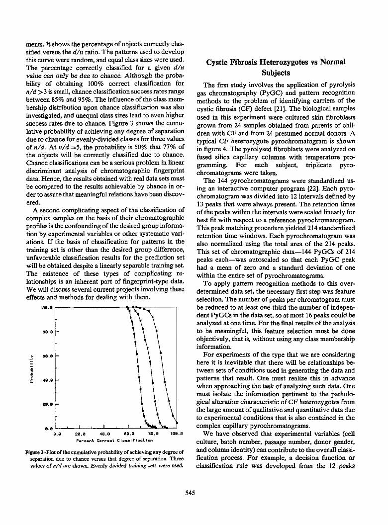
ments. It shows the percentage of objects correctly clas-sified versus the d/n ratio. The patterns used to developthis curve were random, and equal class sizes were used.The percentage correctly classified for a given dinvalue can only be due to chance. Although the proba-bility of obtaining 100% correct classification fornid > 3 is small, chance classification success rates rangebetween 85% and 95%. The influence of the class mem-bership distribution upon chance classification was alsoinvestigated, and unequal class sizes lead to even highersuccess rates due to chance. Figure 3 shows the cumu-lative probability of achieving any degree of separationdue to chance for evenly-divided classes for three valuesof nid. At nid =5, the probability is 50% that 77% ofthe objects will be correctly classified due to chance.Chance classifications can be a serious problem in lineardiscriminant analysis of chromatographic fingerprintdata. Hence, the results obtained with real data sets mustbe compared to the results achievable by chance in or-der to assure that meaningful relations have been discov-ered.

A second complicating aspect of the classification ofcomplex samples on the basis of their chromatographicprofiles is the confounding of the desired group informa-tion by experimental variables or other systematic vari-ations. If the basis of classification for patterns in thetraining set is other than the desired group difference,unfavorable classification results for the prediction setwill be obtained despite a linearly separable training set.The existence of these types of complicating re-lationships is an inherent part of fingerprint-type data.We will discuss several current projects involving theseeffects and methods for dealing with them.

188.9

50.2

a-0

I42.2

28.9

2.22.9 29.9 49.0 62.0 80.2 MA9.9

P.rcrL Corr.o. C1o..lf.ocLon

Figure 3-Plot of the cumulative probability of achieving amy degree ofseparation due to chance versus that degree of separation. Threevalues of n/d are shown. Evenly divided training sets were used.

Cystic Fibrosis Heterozygotes vs NormalSubjects

The first study involves the application of pyrolysisgas chromatography (PyG0) and pattern recognitionmethods to the problem of identifying carriers of thecystic fibrosis (CF) defect [21]. The biological samplesused in this experiment were cultured skin fibroblastsgrown from 24 samples obtained from parents of chil-dren with CF and from 24 presumed normal donors. Atypical CF heterozygote pyrochromatogram is shownin figure 4. The pyrolysed fibroblasts were analyzed onfused silica capillary columns with temperature pro-gramming. For each subject, triplicate pyro-chromatograms were taken.

The 144 pyrochromatograms were standardized us-ing an interactive computer program [22]. Each pyro-chromatogram was divided into 12 intervals defined by13 peaks that were always present. The retention timesof the peaks within the intervals were scaled linearly forbest fit with respect to a reference pyrochromatogram.This peak matching procedure yielded 214 standardizedretention time windows. Each pyrochromatogram wasalso normalized using the total area of the 214 peaks.This set of chromatographic data-144 PyGCs of 214peaks each-was autoscaled so that each PyGC peakhad a mean of zero and a standard deviation of onewithin the entire set of pyrochromatograms.

To apply pattern recognition methods to this over-determined data set, the necessary first step was featureselection. The number of peaks per chromatogram mustbe reduced to at least one-third the number of indepen-dent PyGCs in the data set, so at most 16 peaks could beanalyzed at one time. For the final results of the analysisto be meaningful, this feature selection must be doneobjectively, that is, without using any class membershipinformation.

For experiments of the type that we are consideringhere it is inevitable that there will be relationships be-tween sets of conditions used in generating the data andpatterns that result. One must realize this in advancewhen approaching the task of analyzing such data. Onemust isolate the information pertinent to the patholo-gical alteration characteristic of CF heterozygotes fromthe large amount of qualitative and quantitative data dueto experimental conditions that is also contained in thecomplex capillary pyrochromatograms.

We have observed that experimental variables (cellculture, batch number, passage number, donor gender,and column identity) can contribute to the overall classi-fication process. For example, a decision function orclassification rule was developed from the 12 peaks

545

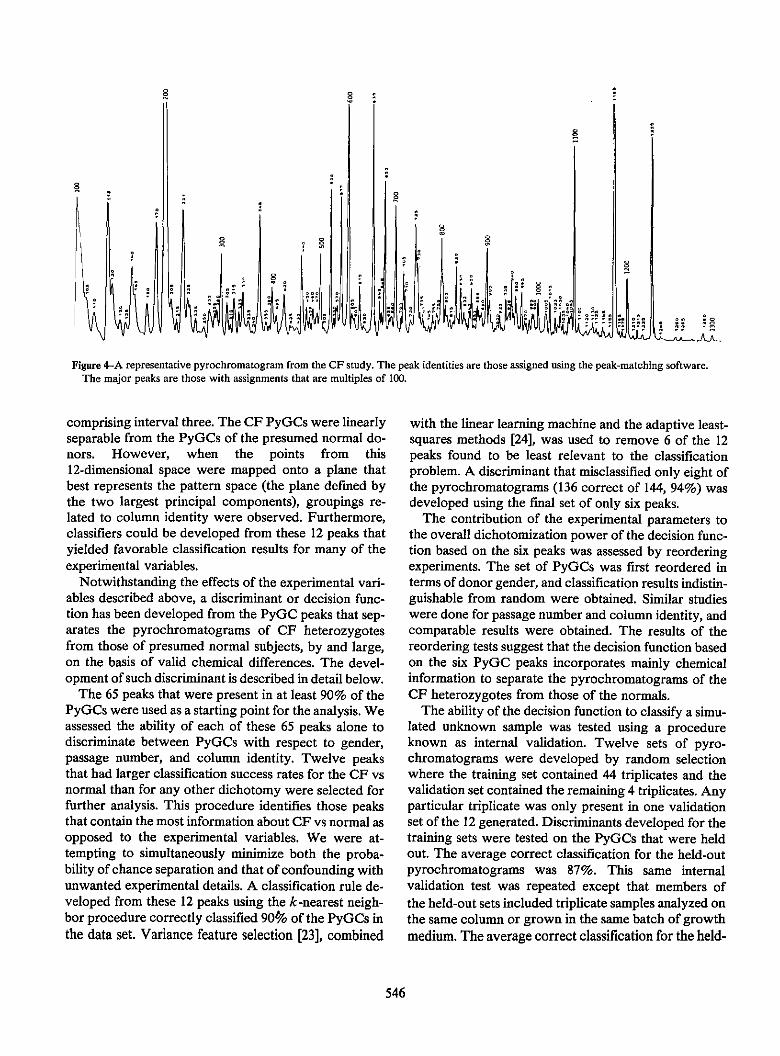
8

r

S

8

Figure 4-A representative pyrochromatogram from the CF study. The peak identities are those assigned using the peak-matching software.The major peaks are those with assignments that are multiples of 100.

comprising interval three. The CF PyGCs were linearlyseparable from the PyGCs of the presumed normal do-nors. However, when the points from this12-dimensional space were mapped onto a plane thatbest represents the pattern space (the plane defined bythe two largest principal components), groupings re-lated to column identity were observed. Furthermore,classifiers could be developed from these 12 peaks thatyielded favorable classification results for many of theexperimental variables.

Notwithstanding the effects of the experimental vari-ables described above, a discriminant or decision func-tion has been developed from the PyGC peaks that sep-arates the pyrochromatograms of CF heterozygotesfrom those of presumed normal subjects, by and large,on the basis of valid chemical differences. The devel-opment of such discriminant is described in detail below.

The 65 peaks that were present in at least 90% of thePyGCs were used as a starting point for the analysis. Weassessed the ability of each of these 65 peaks alone todiscriminate between PyGCs with respect to gender,passage number, and column identity. Twelve peaksthat had larger classification success rates for the CF vsnormal than for any other dichotomy were selected forfurther analysis. This procedure identifies those peaksthat contain the most information about CF vs normal asopposed to the experimental variables. We were at-tempting to simultaneously minimize both the proba-bility of chance separation and that of confounding withunwanted experimental details. A classification rule de-veloped from these 12 peaks using the k-nearest neigh-bor procedure correctly classified 906 of the PyGCs inthe data set. Variance feature selection [23], combined

with the linear learning machine and the adaptive least-squares methods [24], was used to remove 6 of the 12peaks found to be least relevant to the classificationproblem. A discriminant that misclassified only eight ofthe pyrochromatograms (136 correct of 144, 94%) wasdeveloped using the final set of only six peaks.

The contribution of the experimental parameters tothe overall dichotomization power of the decision func-tion based on the six peaks was assessed by reorderingexperiments. The set of PyGCs was first reordered interms of donor gender, and classification results indistin-guishable from random were obtained. Similar studieswere done for passage number and column identity, andcomparable results were obtained. The results of thereordering tests suggest that the decision function basedon the six PyGC peaks incorporates mainly chemicalinformation to separate the pyrochromatograms of theCF heterozygotes from those of the normals.

The ability of the decision function to classify a simu-lated unknown sample was tested using a procedureknown as internal validation. Twelve sets of pyro-chromatograms were developed by random selectionwhere the training set contained 44 triplicates and thevalidation set contained the remaining 4 triplicates. Anyparticular triplicate was only present in one validationset of the 12 generated. Discriminants developed for thetraining sets were tested on the PyGCs that were heldout. The average correct classification for the held-outpyrochromatograms was 87%. This same internalvalidation test was repeated except that members ofthe held-out sets included triplicate samples analyzed onthe same column or grown in the same batch of growthmedium. The average correct classification for the held-

546

out pyrochromatograms in this set of runs was 82%.Although the classification success rate of the decisionfunction was diminished when we took into accountthese confounding effects, favorable results were stillobtained.

Recognition of Ants by Caste and Colony

Chemical communication among social insects can bestudied with chromatographic methods. For example,evidence regarding the role of cuticular hydrocarbonsin nesmmate recognition came from a study of the Myr-mecophilous beetle [251. The data generated in suchstudies can be complex and may require multivariatestatistical or pattern recognition methods for inter-pretation. Presently, we are analyzing gas chro-matographic profiles of high molecular weight hydro-carbon extracts obtained from the cuticles of 179 red fireant (Solenopsin invicta) samples. We are using patternrecognition methods to seek relations with social casteand colony. Each sample contains the hydrocarbons ex-tracted with hexane from the cuticles of 100 individualants. The hydrocarbon fraction analyzed by gas chro-matography was isolated from the concentrated hexanewashings by means of a silicic acid column. Evidenceregarding the role of cuticular hydrocarbons in nest-mate recognition came from a study of the Myr-mnecophilous beetle :25]. A gas chromalographic traceof the cuticular hydrocarbons from a S, invicta sample isshown in figure 5. The hydrocarbon extract was ana-lyzed on a glass column packed with 3% OV-17 usingtemperature programming.

Five major hydrocarbon compounds were identifiedand quantified by GC/MS analysis: heptacosane(ii-C 2 ,HB,), 13-methylheptacosane, 13,15-dimethyl-heptacosane, 3-methylheptacosane, and 3,9-dimethyl-

, a 32 48 64NhO..

heptacosane in the order of elation from the OV-17column used. An internal standard was used for quan-tification. Each chromatograrn was normalized usingthe weight of the collected ants.

Several questions have been addressed in this study:1) Are the hydrocarbon patterns characteristic of indi-vidual colonies? 2) Does the overall colony hydro-carbon pattern change with time? 3) Are the hydro-carbon patterns significantly different for the socialcastes? In this study, ant samples were obtained fromfive different colonies (E, J, P. Q, R), three differentcastes (foragers, broods, and reserves), and for four dif-ferent time periods (the first three in spring and summerand time period four in the winter).

The first step was to use mapping and display methods[12,17] to examine the structure of the data set. Methodsused included principal components mapping and non-linear mapping [141. In figures 6 and 7 the results ofprincipal component mapping experiments for coloniesl and Q are shown. Colony J includes samples from timeperiods one through three, whereas colony Q is repre-sented by ants from all four time periods. Colony J has9 and colony Q has 12 members from each social caste.Pattern groupings according to time period and castecan be seen in figures 6 and 7. The first two principalcomponents account for 96.2% and 97% respectively ofthe total cumulative variance in the two plots shown.Mapping experiments of this nature were also carriedout for samples from a particular caste or time period,and pattern groupings with respect to colony identity,social caste, and temporal period were observed.

I io

.1 V\ tg j~~~~

frmnclpal Componet

Figure 6-Plot of the two principal components of The five GC peaksfor colony J. The elipses show groupigs of samples by time period.

547

Figure 5-Gas crimmatographic trace of cuticular hydrocarbons fromS yvictra (Reprinted with permission from ref. (25D.

Table 1. Percentage of chromatograms correctly classified bycolony for several two-way classifications.

Colony No. in Colony in Second GroupColony E I P Q R All

E 36 - 98 100 100 100 95J 27 - 100 100 100 98P 36 - 100 100 99Q 35 - 73 85R 36 - 82

gression have been employed in this study. The resultsobtained using these techniques support the conclusionsdrawn from the pattern recognition experiments. Insummary, the OC traces representing ant cuticle ex-tracts could be related to colony identity, social caste,and time period using pattern recognition methods.

Figure 7-Plot of the two principal components of the five GC peaksfor colony Q. The foragers are separated from the reserves andbroods by the linear discriminant.

Discriminant analysis studies were also performed. Inone study the data set was divided into three categoriesaccording to the social caste of the pooled ant sample.Linear discriminants were developed using the areas ofthe five GC peaks. The hydrocarbon patterns of theforagers were found to be very different from thebroods and reserves. In fact, information necessary todiscriminate foragers from broods and reserves was pri-marily encoded in the concentration pattern of the firstGC peak. A similar study was undertaken for time pe-riod, and the fourth time period was found to be verydifferent from time periods one, two, and three. Duringtime period four the ants are in a state of hibernation,whereas time periods one, two, and three correspond tothe spring and summer months.

The hydrocarbon profiles were also found to be char-acteristic of the individual colonies. Linear decision sur-faces were developed from the five GC peaks, using aniterative least-squares method. The purpose was to sepa-rate one colony from another or one colony from allother colonies. The results of these discriminant analysisexperiments are summarized in table ]. The first row ofthe table shows that colony E could be separated fromcolony J by a discriminant that achieved 98% correctclassifications (63 correct out of 64 samples) and thatcolony B could be separated from all the remainingcolonies by a discriminant that achieved 95% correctclassifications (162 correct out of 170). Colonies Q andR could not be separated well by this method. In addi-tion, multivariate statistical methods such as multi-variate analysis of variance and stepwise logistic re-

The authors thank J. A. Pino, J. E. McMurry, and R.K. Vander Meer for their helpful contributions.

References

[1] Zlatkis A.; R. S. Brazell and C. F. Poole, The role of organicvolatile profiles in clinical diagnosis, Clin. Chem. 27,789-797(1981).

[2] Jellum, E. J., Profiling of human body fluids in healthy anddiseased states using gas chromatography and mass spec-trometry, with special reference to organic acids, Jour.Chromatog. 143, 427-462 (1977).

(3] Reiner, E., and F. L. Bayer, Botulism: a pyrolysis-gas-liquidchromatographic study, Jour. Chrom. Sci. 16, 623-629(1978).

[4] Reiner, E.,ad J. J. Hicks, Differentiation ofnormal ad pathol-ogical cells by pyrolysis-GLC, Chromatographia 5, 525-528(1972).

[5] Jellum, E.; I. fjoernson, R. Nesbakken, E. Johansson, and S.Wold, Classification of human cancer cells by means of cap-illary gas chromatography and pattern recognition analysis,Jour. Chromatog. 217, 231-237 (1981).

[61 Soderstrom, B.; W. Wold and G. Blomquist, Pyrolysis-gas chro-matography combined with SIMCA pattern recognition forclassification of fruit-bodies of some ectomycorrhizal suillusspecies, Jour. Gen. Micro. 128, 1773-1784 (1982).

[7] McConnell, M. L.; G. Rhodes, U. Watson, and M. Novotny,Application of pattern recognition and feature extractiontechniques to volatile constitutent metabolic profiles ob-tained by capillary gas chromatography, Jour. Chromatog.162, 495-506 (1979).

[8] Wold, S.; E. Johansson, E. Jellum, 1. Bjoernson, andR. Nesbakken, Application of SIMCA multivariate dataanalysis to the classification of gas chromnatographic profilesof human brain tissues, Anal. Chim. Acta 133, 251-259(1981).

[9] Scoble, H. A.; J. L. Fashing and P. R. Brown, Chemometricsand liquid chromatography in the study of acute lympho-cytic leukemia, Anal. Chim. Acta 150, 171-181 (1983).

548

N

C

0

Cs

0.0-

CI.

`4

a a ._ a "

a a

a

a 0

0

Principal Co.pon nt I

[10] Rhodes, G.; M. Miller, M. L. McConnell, and M. Novotny,Metabolic abnormalities associated with diabetes mellitus, asinvestigated by gas chromatography and pattern recognitionanalysis of profiles of volatile metabolites, Clin. Chem. 27,580-585 (1981).

[11] Jurs, P. C., and T. L. Isenhour, Chemical applications of patternrecognition, Wiley-Interncience: New York (1975).

[12] Varmuza, K., Pattern recognition in chemistry, Springer-Verlag: Berlin (1980).

[13] Kryger, L., Interpretation of analytical chemical information bypattern recognition methods-a survey, Talanta 28, 871-887(1981).

[14] Fukunaga, K., Introduction to statistical pattern recognition,Academic Press: New York (1972).

[15] Stuper, A. J.; W. E. Brugger and P. C. Jurs, Computer assistedstudies of chemical structure and biological function, Wiley-Interscience: New York.(1979).

[161 Nilsson, N. J., Learning machines, McGraw-Hill: New York(1965).

(17] Tou, J. T., and R. C. Gonzalez, Pattern recognition principles,Addison-Wesley Pub. Co.: Reading, MA (1974).

[18] Stuper, A. J., and P. C. Jurs, Reliability of nonparametric linearclassifiers, Jour. Chem. Inf. Comp. Sci. 16, 238-241 (1976).

[19] Whalen-Pedersen, E. K., and P. C. Jurs, The probability ofdichotomization by a binary linear classifier as a function oftraining set population distribution, Jour. Chem. Inf. Comp.Sci. 19, 264-266 (1979),

[20] Stouch, T. R., and P. C. Jurs, Monte Carlo studies of the classi-fication made by nonparametric linear discriminant func-tions, Jour. Chem. Inf. Comp. Sci. 25, 45-50 (1985).

[21] Pino, J. A.; J. E. McMurry, P. C. Jurs, B. K. Lavine, and A. M.Harper, Application of pyrolysis/gas chromatography/pattern recognition to the detection of cystic fibrosis hetero-zygotes, Anal. Chem. 57, 295-302 (1985).

[22] Pino, J. A., Pyrochromatography of human skin fibroblasts:normal subjects vs cystic fibrosis heterozygotes, Ph.D. The-sis, Cornell University (1984).

[23] Zander, 0. S.; A. J. Stuper and P. C. Jurs, Nonparametricfeature selection in pattern recognition applied to chemicalproblems, Anal. Chem. 47, 1085-1093 (1975).

[24] Moriguchi, I.; K. Komatsu and Y. Matsushita, Adaptive least-squares method applied to structure-activity correlation ofhypotensive N-Alkyl-N'-cyano-N'-pyridylguanidines, Jour.Med. Chem. 23, 20-26 (1980).

[25] Vander Meer, R. K., and D. P. Wojcik, Chemical mimicry in themyrmecophilous beetle myrmecaphadius excavaticollis, Sci-ence 218, 806-808 (1982).

549